Asset Pricing and Monetary Policy∗

Bingbing Dong†

University of Virginia

First Version: June 2012This Version: January 2013

Abstract

This paper examines the role of money in understanding the behavior of asset prices andwhether and how monetary policy should react to asset prices such as stock prices and equitypremiums. To do so, I introduce money via the form of transaction cost into a productioneconomy with limited stock market participation where agents with lower inter-temporal elas-ticity of substitution (IES), called non-stockholders, have no access to stock market. In additionto facilitating transactions of consumption goods, money also redistributes wealth by counter-cyclically transferring resources from stockholders to non-stockholders, the main role of non-statecontingent bonds. The benchmark model resolves quantitatively the risk premium puzzle andthe risk-free return puzzle, matches macroeconomic behavior such as volatilities of output, con-sumption and investment, and is in line with empirically documented facts about money growth,inflation and asset prices in literature. This model is then used to evaluate alternative policiesfor money growth rates. I find that monetary policies are welfare improving for both stock-holders and non-stockholders if they reduce equity premiums in the economy. These policiesinclude a lower expected money growth, a pro-cyclical money growth rate, and growth rates ofmoney being positively reacting to equity prices or equity premiums, all of which enhance theprecautionary saving role of money.

Keywords: recursive preferences, equity premium, monetary policy, business cycles, elasticlabor supply

JEL Classification Codes: E32, E37, E42, E52, G12

∗I thank Eric Young and Chris Otrok for their invaluable guidance and suggestions with this paper. I alsothank Toshihiko Mukoyama, Kei-Mu Yi, Yili Chien, Thomas Lubik, Max Croce, Roberto N. Fattal Jaef and MartinEichenbaum for their useful comments. I also thank Katherine Holcomb, Ed Hall for their help with Fortran andcomputational questions. All remaining errors are my own.†PhD candidate, Economics Department, P.O. Box 400182, University of Virginia, Charlottesville, VA 22904-4182;

bd3h@virginia.edu; http://people.virginia.edu/˜bd3h/

1

1 Introduction

Whether and how monetary policy should respond to asset prices was for many years a deeplydebatable subject. Though the central banks’ not doing anything with asset prices was a consensusbefore 2007, the recent crisis has now shifted it.1 The recent policy of the Fed, buying securitiesincluding long-term government debt and privately-issued securities, a policy called ”quantitativeeasing”, is definitely an evidence of such a shifting. It is also well-known that even in normaltimes, it is by buying and selling reserves in the interbank overnight market that the Fed conductsmonetary policy, relying on no-arbitrage arguments to link this short-term nominal debt market tothe markets for longer-term bonds and equities. Any model which purports to guide and evaluatethe wisdom of monetary policies should be consistent with the relative prices of the assets inquestion. However, the standard models are quantitative failures at reproducing these relativeprices (for example, the well-known and persistent equity premium and risk-free return puzzles)and thus not reliable to shed light on monetary policies, especially their welfare implications.

This paper contributes to the debate by first developing a model that is consistent with bothmacroeconomic and asset market data. The model is an extension of Guvenen (2009), wherethere are two types of agents, stockholders and non-stockholders, in a production economy. Thestockholders, as smaller fraction of total population, have access to both the stock market andbond market, while the non-stockholders are restricted to the latter. Both of them are allowedto borrow only a certain amount based on their wage income. They both have Epstein-Zin-Weilpreferences (Epstein and Zin, 1989; Weil, 1990), which disentangle risk aversions from the elasticityof intertemporal substitution (EIS). Consistent with empirical evidence, the non-stockholders, whohave relatively lower wealth, are assumed to have a low EIS, whereas the stockholders have a higherelasticity. There is one external firm, whose share is normalized to be 1, that can produce withcapital and labor, subject to capital adjustment cost.

Money is introduced via transaction costs on consumption, taking the form of real resourcesthat are consumed during the process of exchange (Brock, 1974, 1990; Schmitt-Grohe and Uribe,2004). That is, given a volume of consumption goods, higher money balance helps reduce the costof consumption. It turns out that adding money is important. First, money is one type of assets,meaning that it has to be properly priced as others like bonds and stocks via no-arbitrage. Indeed,since money now competes with bonds in the role of saving intertemporally, it is harder for themodel to match asset pricing facts such as a high and countercyclical equity premium. It points outthat the model of Guvenen (2009) is not robust if introducing another asset. Second, since moneyis distributed equally to the agents as a lump-sum transfer and the wealth and preferences of thoseagents differ, it has real effects on macro fundamentals and hence asset prices through portfolioreallocation. Therefore, money is non-neutral. The Central Banks conduct monetary policy byvarying money growth rates.

This model is remarkably good in matching asset price and macroeconomic data with plausiblecalibrations. It produces higher equity premium and lower risk-free return, 5.3% and 1.6% perannum, respectively. In particular, the match of Sharpe ratio (0.25 vs 0.32 in the data) shows thatthe risks in the economy are appropriately evaluated. Compared with the literature, the model alsoperforms better in matching volatilities of output growth, the relative volatilities of consumptionand investment. Finally, the model is in line with empirically documented relationship betweenmoney growth, inflation and asset prices. Specifically, the decrease of expected inflation (moneygrowth rate) explains partially the decline of equity premiums during the past three decades.Unexpected inflations due to real shocks are negatively related with stock prices, real stock returns

1See Bernanke and Gertler (2001), for example.

2

and real risk-free returns.I then use this model to evaluate alternative monetary policies: (1) a change of average money

growth rates; (2) a money growth rate reacting to business cycles; (3) a monetary policy respondingto equity prices; and (4) a policy reacting to expected risk premiums. All the experiments arecompared with a representative agent model with similar setups to shed light on the innovationsof having assets appropriately priced. In stark contrast with the conventional wisdom of Friedmanrule, my model shows that the monetary policies yield welfare improvements for all types of agentsif it drives down the equity premiums. This corresponds to a policy with lower expected inflation,a pro-cyclical monetary policy, and policies that positively responding to stock prices and equitypremiums.

This paper relates to a large literature discussing monetary policies and asset prices. Bernankeand Gertler (2001) shows in a small scale macro model that asset prices become relevant onlyto the extent they may signal potential inflationary or deflationary forces and rules that directlytarget asset prices appear to have undesirable side effects. Bullard and Schaling (2002) constructa model showing that asset prices targeting can interfere with the minimization of inflation andoutput variation and under certain conditions, asset price targeting can lead to indeterminacy. Onthe other hand, Cecchetti (1997), Blanchard (2000), and Mishkin (2000) claimed that consideringasset prices improved economic performance. After the crisis, it is now increasingly accepted that,to some degree and extent, mainstreaming reactions to asset price moves in monetary policy isto become a new norm.2 Rudebusch et al. (2007) point out that changes in the term premium ofbonds has real effects to the economy. Gallmeyer et al. (2007), and Palomino (2010) show that termstructure and endogenous inflation are important for understanding monetary policies. Paoli andZabczyk (2012) shows that the varying precautionary saving due to cyclical risk aversion chouldlead to large policy errors in turbulent times. However, none of these works or suggestions has beenbuilt on a structural model that explains the asset prices data quantitatively. It is therefore likelyto misestimate the effects of considering asset prices in monetary policies.

This paper relates to a growing literature that jointly studies asset prices and macroeconomicbehavior. Besides Guvenen (2009), many other papers deal with the same problem, includingDanthine and Donaldson (2002), Storesletten et al. (2007), Tallarini (2000), etc. However, moneyis not considered in any of these models. Earlier papers that discuss the relationship betweenmoney and asset prices includes Danthine and Donaldson (1986), Marshall (1992), Labadie (1989),Boyle (1990), Balduzzi (1996) and Hodrick et al. (1991), all of which focused on an endowmenteconomy. In particular, Bansal and Coleman (1996) explain equity premium by examining money’srole in facilitating transactions. This idea then is inherited by Gust and Lopez-Salido (2010), whoconsider market segmentation in checking and brokerage account. These two accounts are differentin liquidity and infrequent portfolio rebalance leads to the high volatility in consumption for thosewho are active and then compensated by high risk premium. They show that this model can matchsome statistics of asset prices and then discuss the welfare gains for different monetary policies.However, they do not explore the performance of the model in matching macroeconomic behavior.

There is also a large literature documenting the relationship between money growth, inflationand asset prices. For example, inflation is negatively correlated with real stock prices if the economyis driven by supply shocks; see Tatom (2011) and Christiano et al. (2010).3 Also the negativerelationship between inflation and asset returns is in the spirit of research in finance initiated inthe early 1980s. Geromichalos et al. (2007) study the effect of monetary policy on asset prices inan endowment economy with search-based money. When money grows at a higher rate, inflation

2See Canuto (2009), Issing (2009), and Kohn (2007), etc.3Since inflation is low during stock market booms, so that, Christiano et al. (2010) claim, an interest rate rule

that is too narrowly focused on inflation destabilizes asset markets and the broader economy.

3

is higher and the return on money decreases. In equilibrium, no arbitrage amounts to equatingthe real return of both objects. Therefore, the price of the asset increases in order to lower its realreturn.

It is also claimed that the decrease of equity premium during the Great Moderation is due tothe decline of inflation; See Siegel (1999), Jagannathan et al. (2000), Claus (2001), and Campbell(2008) for the evidence of decreasing premia and see Beirne and de Bondt (2008) and Kyriacou et al.(2006) for empirical estimation of inflation’s role in mitigating premia.4 Labadie (1989) explorestwo ways that inflation affects equity premium in a theoretical model. However, her model is basedon an endowment economy. In contrast to her conclusion, my paper shows that it is the expectedinflation, not the unexpected one, that determines or closely relates to the equity premium.

The paper is organized as follows. The next section presents the model with solution methodsand computational algorithm discussed in section 3. Section 4 explores the role of money inreconciling asset pricing and macroeconomic facts. Section 5 is devoted to policy analysis. Section6 concludes.

2 The Model

The economy studied is based on the framework of Guvenen (2009). Money is introduced via atransaction cost, taking the form of real resources that are consumed in the process of exchange(Brock, 1974, 1990; Schmitt-Grohe and Uribe, 2004). That is, an increase in the volume of goodsexchanged leads to a rise in transaction costs, while higher average real money balances, for a givenvolume of transactions, lower costs. Compared with other alternative approaches for money inmacroeconomics and policy analysis, this setup loosens the tight relationship between money andconsumption.5

2.1 The Central Bank

In each period t, the central bank issues some new money (gt−1)M st−1 and gives it to the agents as

a lump-sum transfer. M st is the per capita money supply in the economy. The money stock follows

a law of motionM st = gtM

st−1, (1)

where gt is the gross growth rate of money supply. The growth rate of the money supply evolvesfollowing:

log(gt) = (1− ρg) log(g) + ρg log(gt−1) + (2)

θy log(Yt/Y ) + θEP log(EtREPt+1/R

EP) + θPE log(P st /P

s) + εg,t

In equation (2), εgiid∼ N(0, σ2g), log(g) is the unconditional mean of the logarithm of the growth

rate gt, Y , REP , and P s are the averages of output, equity premium and stock prices, respectively.This rule allows for a systematic response of money to changes in output, expected equity premium(implied future risks) and equity prices. I evaluate four simple rules: (1) constant money growth

4Others claim that it can be due to the declining volatility of technology shocks or other possible shocks/structuralchanges; see Lettau et al. (2008), for example. .

5Wang and Yip (1992) proved the ”functional equivalence” between the transactions cost and other approacheslike MIU, CIA and shopping time models that are commonly used in macroeconomics and policy analysis. There isanother category of money modelling aiming to understand the microfoundation of money, such as search theoreticmodels by Kiyotaki and Wright (1989) and Nosal and Wright (2010).

4

when ρg = θy = θEP = θPE = 0; (2) monetary rules that are either procyclical (θy > 0) orcountercyclical (θy < 0) when ρg = θEP = θPE = 0; (3) rules that respond to equity premiumswhen ρg = θy = θPE = 0 and θEP 6= 0; and finally (4) rules that respond to equity prices whenρg = θy = θEP = 0 and θPE 6= 0.

2.2 Households

There are two types of households who live forever in the economy. The population is constantand normalized to be unity. Let µ ∈ (0, 1) denote the measure of stockholders and 1 − µ non-stockholders. Each of them is endowed with one unit of time every period, which he allocatesbetween market work and leisure. They both have Epstein-Zin-Weil preferences (Epstein and Zin,1989; Weil, 1990) with the following form:

U it =

[(1− β)uit + β(E(U it+1)

1−σi)ρi

1−σi

] 1

ρi

(3)

for i = h, n, where throughout the paper the superscripts h and n denote stockholders and non-stockholders, respectively; uit is current utility, a function of consumption cit and labor lit. Theconventional interpretation is that ρi < 1 governs the intertemporal substitution (EIS is 1/(1−ρi))and σi governs relative risk aversion.

The stockholders choose consumption (cht ), bond holdings (bht+1), stock shares (st+1), and nom-inal money holdings (mh

t ) subject to the following budget constraint:

cht + P ft bht+1 + P st st+1 +

mht

Pt+ Ψ(ct,

mht

Pt) ≤ bht + st(P

st +Dt) +Wtl

ht +

mht−1 + (gt − 1)M s

t−1Pt

(4)

where the right side is all the real sources that can be spent. It includes values of holding bondand shares, bht + st(P

st + Dt), wage income, Wtl

ht , and money carried over from previous period,

mht−1, plus the lump-sum transfer from the central bank (gt − 1)M s

t−1, divided by the price ofgoods, Pt. Stock prices, P st , and dividend, Dt, are defined in details in the following subsection.Non-stockholders have a similar budget constraint except that they do not own stocks and thus donot choose st+1.

In equation (4), I introduce real money demand by having the transaction cost Ψ, which isa function of consumption c and real money balances m/P . Feenstra (1986) demonstrates thatthe transaction costs satisfy the following condition for all c,m/Pc ≥ 0: Ψ is twice continuouslydifferentiable and Ψ ≥ 0; Ψ(0,m/P ) = 0; Ψc ≥ 0; Ψm/P ≤ 0; Ψcc,Ψm/P,m/P ≥ 0; Ψc,m/P ≤ 0; andc+ Ψ(c,m/P ) is quasi-convex, with expansion paths having a nonnegative slope.67

2.3 The Firm

There is an aggregate firm producing a single good that can be used for either consumption orinvestment by using capital (Kt) and labor (Lt) inputs according to a Cobb-Douglas technology:

6If no firm leverage (detailed below), then a portfolio adjustment cost for bonds has to be added. Whenever theagents change their bond positions, they incur a cost of φ

2(bht+1/b

ht − 1)2, where φ is the semi-elasticity of adjustment

cost over changes. The necessity for adding this cost is that money essentially has a similar feature as bonds, whichis more risk-free when no leverage. By facilitating goods transactions, it gives the agents an implicitly determinedreturn which is nearly risk-free. Hence, it makes no difference for a household to choose between bonds and money.By adding such a cost, assets in the economy have a nonsingular return matrix and hence the agents can distinguishbonds from money when making a decision.

7Tough with different forms of the functional form, money has been introduced in this approach widely in theliterature, see Sims (2003), Schmitt-Grohe and Uribe (2004), etc.

5

Yt = ZtKθt Lt

1−θ, where θ ∈ (0, 1) is the factor share parameter. The productivity level evolvesaccording to:

log(Zt+1) = ρz log(Zt) + εz,t+1, εziid∼ N(0, σ2z) (5)

The objective of the firm is to maximize the value of the firm, which equals the value of futuredividend stream generated by the firm, {Dt+j}∞j=1, discounted by the marginal rate of substitutionprocess of stockholders, {Λt,t+j}∞j=1. Specifically, the firm’s problem is to solve:

P st = max{It+j ,Lt+j}

Et

∞∑j=1

Λt,t+jDt+j

(6)

subject to the law of motion for capital, which features adjustment costs in investment:

Kt+1 = (1− δ)Kt + Φ(ItKt

)Kt (7)

where P st is the ex-dividend value of the firm. The number of shares outstanding is normalized tounity for convenience and hence P st is the stock price. Strict convexity of Φ(·) captures the difficultyof quickly changing the level of capital installed in the firm, which is necessary if the model is togenerate realistic asset prices, particularly equity prices; see Cochrane (1991). An equity share isthe right to own the entire stream of dividends, defined by the profits net of wages and investments:Dt = ZtK

θt (Lt)

1−θ −WtLt − It − χK.8

2.4 Financial Markets

There are two types of assets traded in this economy: a one-period bond and an equity share (stock).The non-stockholders can freely trade the risk-free bond while restricted from participating in thestock market. In contrast, the stockholders have access to both markets and hence are the solecapital owners in the economy. As in Guvenen (2009), portfolio constraints are imposed to avoidPonzi schemes.

2.5 Individuals’ Dynamic Problem and Equilibrium

A change in variables is introduced so that the problem solved by the households is stationary.That is, let m̂i

t = mit/M

st and P̂t = Pt/M

st . In addition, I let m̂i = m̂i

t−1 be the money balances ofagent i at the beginning of period t. In each given period, the portfolio of each group is a functionof the beginning-of-period capital stock, K, the aggregate bond holdings of non-stockholders afterproduction, B, the beginning-of-period aggregate money holdings of non-stockholders, M̂, the grossrate of money supply, g, and the technology level, Z. Let Υ denote the aggregate state vector(K,B, M̂, Z, g). The dynamic programming of a stockholder can be expressed as follows (primesindicate next period values):

V h(ωh; Υ) = maxch,lh,bh′,sh′,m̂h′

[(1− β)u(ch, lh)ρ

h+ β(E(V h(ωh′; Υ′)|Z, g)1−σ

h)

ρh

1−σh

] 1

ρh

(8)

8Guvenen (2009) claims that (in his note 4) the existence of leverage has on effect on quantity allocations. However,this is not true when money, a competing asset, is introduced (?).

6

s.t.

ωh +W (Υ)lh ≥ ch + P f (Υ)bh′+ P s(Υ)s′ +

m̂h′

P̂ (Υ)+ Ψ(c,

m̂h′

P̂ (Υ)) (9)

ωh′ = b′ + s′(P s(Υ′) +D(Υ′)) +m̂h′ + g′ − 1

P̂ (Υ′)g′(10)

K ′ = ΓK(Υ), B′ = ΓB(Υ), M̂ ′ = ΓM̂

(Υ) (11)

bh′ ≥ B (12)

where ωh denotes financial wealth; bh and s are individual bond and stock holdings, respectively;ΓK , ΓB and Γ

M̂denote the laws of motion for the wealth distribution which are determined in

equilibrium; and P f is the equilibrium bond pricing function. The problem of a non-stockholdercan be written as above with s′ ≡ 0, and the superscript h replaced with n.

A stationary recursive competitive equilibrium for this economy is given by a pair of valuefunctions, V i(ωi; Υ); consumption, labor supply, bond holding decision rules and money holdingdecision rules for each type of agent, ci(ωi; Υ), li(ωi; Υ), bi′(ωi; Υ), and m̂i′(ωi; Υ); a stockholdingdecision rule for stockholders, s′(ωi; Υ); stock, bond and consumption goods pricing functions,P s(Υ), P f (Υ), and P̂ (Υ); a competitive wage function, W (Υ); an investment function for thefirm, I(Υ); laws of motion for aggregate capital, aggregate bond holdings of non-stockholders, andaggregate money holdings of non-stockholders, ΓK(Υ),ΓB(Υ), and Γ

M̂(Υ); and a marginal utility

process, Λ(Υ), for the firm such that:(1) Given the pricing functions and laws of motion, the value function and decision rules of each

agent solve that agent’s dynamic problem.(2) Given W (Υ) and the equilibrium discount rate process obtained from Λ(Υ), the investment

function I(Υ) and the labor choice of the firm, L(Υ), are optimal.(3) All markets clear: (a) µbh′(ωh; Υ)+(1−µ)bn′(ωn; Υ) = 0 (bond market); (b) µs′(ωh; Υ) = 1

(stock market); (c) µlh(ωh; Υ) + (1 − µ)ln(ωn; Υ) = L(Υ) (labor market); (d) µm̂h′(ωh; Υ) + (1 −µ)m̂n′(ωn; Υ) = 1 (money market); and (e) µ[ch(ωh; Υ) + Ψ(ch(ωh; Υ), m̂h′(ωh; Υ)/P̂ (Υ))] + (1 −µ)[cn(ωn; Υ) + Ψ(cn(ωn; Υ), m̂n′(ωn; Υ)/P̂ (Υ))] + I(Υ) = Y (Υ) (goods market), where ωi denotesthe wealth of each type of agent in state Υ in equilibrium.

(4) Aggregate laws of motion are consistent with individual behavior: (a) K ′ = (1 − δ)K +

Φ(I(Υ)/K)K; (b) B′ = (1− µ)bn(ωn,Υ); and (c) M̂ ′ = (1− µ)m̂n(ωn,Υ).(5) There exists an invariant probability measure P defined over the ergodic set of equilibrium

distributions.9

3 Quantitative Analysis

3.1 Solution Methods

The solution method used is a direct application of policy function iteration proposed by Cole-man (1989, 1990). This gives a global solution over the entire state space. There are two othermethods that are popular for solving this class of models. The first one is value function iterationmethod, which is used by Krusell and Smith (1997), Storesletten et al. (2007) and Guvenen (2009),among others. The application of this method to incomplete asset pricing models is computation-ally inefficient. The second one can be roughly categorized as approximation methods, including

9Details for solving the model are in Appendix B.

7

loglinear approximation (e.g. Backus et al. 2007, 2010), affine method (e.g. Shamloo and Malkho-zov (2010)), perturbation methods (e.g. Malkhozov and Shamloo, 2009b; Kim et al. (2005)). Theproblem with this method is that it gives local solutions around where you approximate (usually,the steady state). When the problem of interest is actually not in steady state, the local solution isuseless. Second, the far away from the steady state, the bigger the approximation errors are. Thismay give you misleading policy functions and particularly underestimate the fluctuations in assetprices, which is important for explaining asset pricing facts.

To solve the model, I substitute individual state variables out and keep only aggregate statevariables. The new system of equations then is used as an input for the solver. The computationalalgorithm is detailed in Appendix B. It turns out my algorithm is much faster than that of Guvenen(2009). A test of running the model without money takes about 250 hours on a 3-GHz Intel dual-core Xeon cpu by his algorithm while mine only several minutes.

3.2 Baseline Parameterization

A model period corresponds to one month of calendar time. Table 1 summarizes the baselineparameter choices. I start with the parameterization of productivity and money growth. As forthe technology shock, the AR(1) coefficient ρz is set to be 0.976 at monthly frequency in order tomatch the 0.95 autocorrelation of Solow residuals at quarterly frequencies. The standard deviationσz is set to be 0.015 to match the standard deviation of H-P filtered output in quarterly data.Similarly, ρg is set to be 0.17 at monthly frequency to match the 0.005 autocorrelation of M0growth rate in US data. For the benchmark model, g is set to be 1.0025 to match a 3% annualinflation. The variance of money growth, σg, is set to be either 0 for only expected inflation or0.0045 for unexpected inflation.

EIS parameters for stockholders and non-stockholders are set to be 0.3 and 0.1, respectively.10

I set discount factor β to be 0.93 to get 1.69% risk-free return in the benchmark model. I then setdepreciation rate δ = 0.02, capital share θ = 0.36 to roughly match the US capital-output ratio of 8in quarterly data. Capital adjustment cost coefficient is set to be 0.99 to match relative volatilitiesof consumption and investment over output.11 Participation rate and borrowing constraints arethe same to those in Guvenen (2009).

Table 1 here!

3.2.1 Portfolio Adjustment Cost

It deserves special discussion on choosing the value of φ, which governs how costly households adjusttheir bond positions. Theoretically, φ can be calibrated by the ratio of value added by financialdepartment over GDP in national income account, which is approximately 5% in US. However,changing the value of φ gives no difference in the model economy and the simulated results showthat the ratio of cost incurred over output is always negligible and close to 0.12 Nevertheless, sucha cost must exist to make bonds perform different from money in the sense of getting risk-freereturn. By experimenting with different values, I find that φ should be bigger than 0.1. Here I setit to be 1 for simplicity.

10However, debates about the right values for these parameters persist. See Guvenen (2006), Blundell et al. (1994),among others.

11Capital adjustment cost function takes the form of Φ(It/Kt) = a1(It/Kt)1−1/ξ + a2, where a1 = δ1/ξ

1−1/ξ, and

a2 = δ1−ξ . The parameter ξ governs how easily investment can be transformed into capital.

12Some others also find that this cost typically is very small, though they have a different modeling setup. Forinstance, Barber and Odean (2000) calculate a similar cost varying from 0.01% to 0.1% of the portfolio value.

8

3.2.2 Utility Functions

I consider two different specifications for the current utility function. First, I begin with the casewhere labor supply is elastic as a benchmark. The current utility therefore takes the form ofGreenwood et al. (1988):

u(cit, lit) =

[cit − ψ

(lit)ξ

ξ

]ρi(13)

where lit is the labor supply of each agent at period t. There is no uniform agreement about thecorrect value of the Frisch elasticity 1

ξ−1 . So I set it to be 1/3 for the benchmark model and trydifferent values, including an estimate of 1 from Kimball and Shapiro (2003), to see the modelperformance. Finally, ψ is chosen to match a target value of L = 0.33. In order to provide a simplecomparison, I also consider the case with inelastic labor supply and assume that current utility

function is of the standard power form: u(cit, lit) = ciρ

i

t .

3.2.3 Transaction Cost of Consumption

The transaction cost function takes the following form:

Ψ(c,mi

P) = ζc exp(−αm

i

Pc)

where ζ and α are positive constants. One can prove that this form satisfies all the conditionsclaimed by Feenstra (1986).13 Here we treat it as the cost of maintaining the ATM/paymentsystem. To calibrate ζ and α, we use the data from the FRED database of Federal Reserve Bank ofSt. Louis: Consumption is real monthly expenditures on nondurables (PCENDC96) and services(PCESC96); the money supply is M0 (CURRSL); real balances are the money supply dividedby GDP deflator (GDPDEF). The average monthly expenses for one ATM are roughly $1450 in2006.14 In the same year, the total number of ATM used in US is 395, 000.15 All quantity variablesare divided by the resident U.S. population (CNP16OV). Our first goal is to match the averagetransaction cost, which is 1.2% of conumption goods.1617

Following Robert E. Lucas (2000) and Ireland (2009), the second goal is to match the moneydemand elasticity on interest rate with the following form:

ln(m) = ln(B)− ξr,

where ξ̂ = −1.88 is estimated from the data. We vary the values of ζ and α to match these twotargets and get ζ = 0.05 and α = 0.6, respectively.

13Note that we are using a different form from those used in Bansal and Coleman (1996) and Marshall (1992),where a power function is used. The reason that we use the exponential form rather than the power form is thatit avoids the possibility of such a solution that one agent holds negative money balance in the latter case. Also thedefinition of transaction cost is different from Schmitt-Grohe and Uribe (2004).

14Data source: 2006 ATM deployer study.15See http://www.creditcards.com/credit-card-news/atm-use-statistics-3372.php .16Humphrey et al. (2003) have a different estimation of the cost of payment system and the benefit from using

more ATMs.17Marshall (1992) estimates a 0.8% cost of output. Barber et al. (2009) use a complete trading history of all

investors in Taiwan and find that individual investor losses are equivalent to 2.2 percent of Taiwan’s GDP or 2.8percent of total personal income.

9

4 The Role of Money in Asset Pricing

Table 2 shows the performance of the benchmark model. Compared with the literature, I have gota better matching to the basic asset pricing and business cycle facts. Equity premium is 5.29%percent a year while risk-free return is 1.69%. It also delivers a Sharpe ratio (0.25) close to thatin the data (0.32). While the variances of output growth, the relative volatility of investment areclose to those in the data, volatilities of consumption and labor are not so well matched, whichhave been found hard to match in the literature.

Table 2 here!

The model is also consistent with what are empirically documented about the relations betweeninflation and asset prices, given the source of inflation is technology shocks. For example, Tatom(2011) documents that Inflation and real stock prices are negatively correlated, depending on thesources of inflation. This relation is mostly apparent during Great Inflation, 1965-84. Giovanniniand Labadie (1991) documents that when inflation is high, realized real stock returns and interestrates are low, and vice versa. The main channel here is via no-arbitrage between money and otherreal assets. Table 3 reports that a negative relationship between inflation and real stock prices,real stock returns and real interest rates. The comovement of inflation and nominal interest rate isno surprise. Finally, the model gives a very high negative correlation between inflation and equitypremiums, which might be debatable. The logic of this high relation is: Suppose these a positiveshock, output is high and hence the equity price, which leads to high stock prices; at the sametime, non-stockholders require a lower risk-free return to save because their marginial utility ofconsumption is lower; given that money supply is constant, a lower price level (inflation) followed.

Table 3 here!

5 The Determinants of Declining Equity Premium

It is widely documented that the equity premium has been going down during the last threedecades, the so-called Great Moderation; see Siegal (1999), Jagannathan et al. (2000), Clause andThomas (2001), and Campbell (2007). However, the reason for such a trend is still on debate.Besides a declining volatility of technology shocks and improvement of market imperfection, onecompeting explanation is that this is due to the decrease of inflation since sustained low inflationimplies less uncertainty about the future.18 Beirne and de Bondt (2008) claims that these two areclosely related. Kyriacou et al. (2006) shows that inflation can exaggerate equity premium. Labadie(1989) established a endowment economy model to explore the two ways of inflation to affect equitypremium, namely by the assessment of an inflation tax and the presence of an inflation premium.

Here I explore the role of decreasing inflation by experimenting with different money growthrates. Table 4 shows that the decrease of inflation is one source of the declining equity premium.However, the equity premium goes down only 0.02 − 0.1 percent by one percent decrease in infla-tion.19 Given the the inflation decreased from an average of 8% to 2%, the decline that can be

18See Campbell and Vuolteenaho (2004), Ritter and Warr (2002), Lettau et al. (2008), for example.19It needs mention that it is the expected inflation, not the unexpected one, that determines or closely relates to

the equity premium, in contrast with Labadie (1989).

10

explained by inflation is only approximately 0.22 percent.20 Also note that as inflation goes higher,its role in driving equity premium is deteriorating. This shows that hyperinflations do not lead toinfinitely higher equity premia.

Table 4 here!

The reason is that money has two roles, transaction and intertemporal saving. As money growth(inflation) becomes higher, money’s role for saving will be dominated by bonds, which means thatthe demand curve for money has a kink as money growth rate is higher. The role of money indriving down the equity premium can also be seen by the Euler equations that price bonds andstocks. The pricing kernel of the stockholders is

Mht+1 = β

V ht+1

[EtVh1−σht+1 ]

1

1−σh

1−ρh−σh (cht+1

cht

)ρh−11 + Φ′(m̂h

t /P̂tcht )

1 + Φ′(m̂ht+1/P̂t+1cht+1)

(14)

andEtM

ht+1R

EPt+1 = 0 (15)

where REPt+1 =P st+1+Dt+1

P st− 1

P fis the equity premium. From equation (15) we get EtMt+1EtR

EPt+1 +

Cov(Mht+1, R

EPt+1) = 0, 21 where we conclude that money matters because Mh

t+1 depends on moneygrowth via portfolio reallocation and so does Cov(Mh

t+1, REPt+1).

22 Since the real value of money isonly a small fraction of agents’ wealth, its role in resolving equity premium puzzle is limited. Asmoney growth goes up, the real value of money carried from previous period, m̂

i

P̂ g, is decreasing with

a slower rate, and thus inflation drives up less and less equity premium. That is, as money growthrate goes up, the uncertainty induced by inflation is decreasingly declining.

6 The Welfare Effects of Money: Quantitative Estimations

Compared with a standard classic model, this section answers the following two questions:23 First,what is the optimal money growth rate? Second, should monetary policy be countercyclical orrespond to asset prices, such as equity prices or expected equity premium? We answer these twoquestions by comparing the welfare under different policy regimes. Specifically, suppose V B(Υ)and V A(Υ) are the value functions for the benchmark and under the alternative monetary polices.The welfare change is measured as percentage change of consumption in the benchmark, that is,to find τ such that

V A(Υ) = V B(Υ)(1 + τ) (16)

≡[(1− β)u(c(1 + τ), l)ρ + β(E(V (ω′; Υ′)|Z, g)1−σ)

ρ1−σ] 1ρ

20Tough it is not the theme of this paper to estimate contributing role of the declining variance of technologyshocks, a rough estimation shows that it explains most of the decrease in equity premium. It can be shown that

inflation depends approximately on the ratio of money growth rate to technology growth rate, i.e., π ∝ gM

gcwhere

gc ≈ 1/3gz; and hence, π ∝ 3 gM

gz, which shows that change of gz plays a more important role.

21Equity premium is thus EtREPt+1 = −Cov(Mh

t+1, REPt+1)/EtMt+1.

22In the representative agent model as I present in Appendix A, the pricing kernel becomes Mt+1 =

β

(Vt+1

[EtV1−σt+1 ]

11−σ

)1−ρ−σ (ct+1

ct

)ρ−11+Φ′(1/P̂ c)1+Φ′(1/P̂ ′c)

, which is not affected by the injection of money.

23See Appendix A for the conterpart of the model presented in this paper, which is a representative agent model.

11

In doing so, we can get the welfare change for each state vector Υ. I then simulate a longtime-series (T = 50, 000) under the benchmark and then calculate the average welfare change τ . Ifτ is positive (negative), then we say there is a welfare gain (loss).

6.1 The Optimal Money Growth Rate

In the last section, we have concluded that risk premia are of different size since different moneygrowth rates deliver different risks and, in particular, different risk-sharing allocations in the econ-omy. Table 5 reports the welfare implications of different expected money growth rates, comparingwith the zero-inflation case.

Table 5 here!

As shown in the table, the total welfare, the welfare of stockholers and non-stockholers aredecreasing with inflation rates. Therefore, zero money growth rate is not optimal. In contrast,a deflation is welfare improving. The logic is that now there is less uncertainty about inflation,and thus less precautionary saving motivation from non-stockholders, which then means that theyconsume more and buy less bonds. Stockholders now have to pay higher return to borrow, butthey also borrow less. The equilibrium is that both of them better off.

6.2 Implications of Alternative Monetary Polices

This subsection considers three alternative monetary policies, compared with the benchmark model.The first case is whether monetary policies should be procyclical or countercyclical, where we setρg = θEP = θPE = 0 and θy = −0.05,−0.025,−0.01, 0.01, 0.025, 0.05, respectively. Figure 1 showsthe equity premia and risk-free returns with each parameter values. It turns out that procyclicalpolicy tends to drive up risk-free return and down the equity premium, where equity returns are ofalmost no changes. The welfare change is shown in Panel A of Table 6. In contrast with the popular”leaning against the wind” advice, I find that procylical monetary policy is welfare-improving. Thelogic is similar as in the last subsection. Procyclical money injection makes the saving role ofmoney stronger and holding money now is less risky, which amounts to less uncertainty aboutinflation. Higher return of money tranmits to higher return on bonds and lower equity premiumvia no-arbitrage.

Figure 1 here!

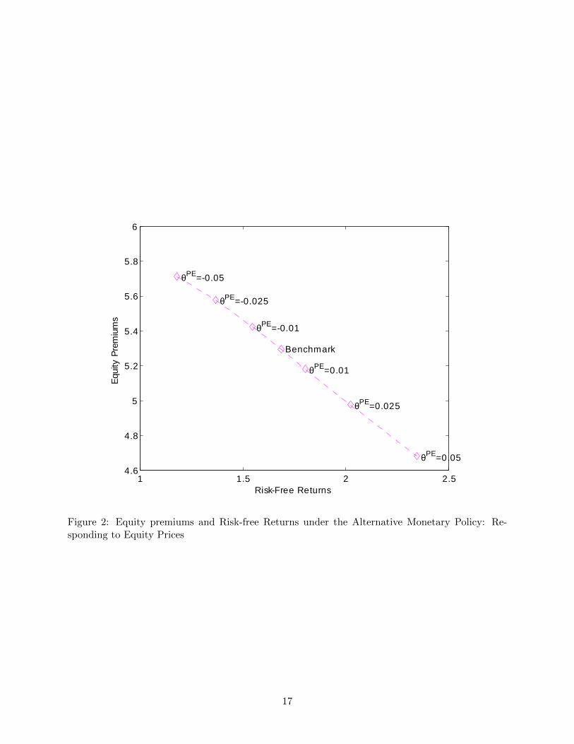
The second is to explore whether monetary policy should respond to asset prices, say realequity prices. In this case, ρg = θy = θEP = 0 and θPE = −0.05, −0.025, −0.01, 0.01, 0.025, 0.05,respectively. Figure 2 shows again the equity premia and risk-free return with different coefficientsof monetary policy responding to equity prices. Welfare implications are similar to the rules reactingto business cycles, as shown in Panel B of Table 6. The reason for this result is that asset pricesare highly correlated with output (corr(P st , yt) ≈ 0.999).

Figure 2 here!Table 6 here!

Finally, I consider the case where monetary policy responds to (expected) equity premiums.If equity premium is high, policy makers view that there is higher risk in the economy and thusmop it down by setting θEP positive, which is a countercyclical policy. Without surprise, such apolicy drives down equity premium and thus improves the welfare of the whole economy, as shownin Figure 3 and Panel C of Table 6.

12

Figure 3 here!

7 Conclusion

This paper first builds a monetary model with production and limited stock participation to recon-cile with asset prices and macroeconomic data. Specifically, it not only resolves the equity premiumand risk-free return puzzles, matches volatilities of macro fundamentals, but also is in line withempirical findings about the relations among inflation, money growth rate and asset prices.

This model is then used to estimate alternative monetary policies, compared with a standardclassic model where there is only one representative agent model. In contrast with conventionalwisdom of Friedman rule, saying optimal inflation should be the negative of real returns on otherassets, this paper shows that monetary policies are welfare improving if they drive down the equitypremium and raise risk-free returns. This manifests a procyclical monetary policy, a positiveresponse of monetary policy to stock prices and risk premiums.

Appendix A: The Representative Model

There is only one stand-in household who live forever in the economy. The population is normalizedto be unity, who is endowed with one unit of time every period, which he allocates between marketwork and leisure. The agent has similar Epstein-Zin-Weil preference as in the heterogeneous model:

Ut =[(1− β)ut + β(E(Ut+1)

1−σ)ρ

1−σ] 1ρ

(A1)

where ut is again current utility, a function of consumption ct and labor lt. The household has asimilar budget constraint as stockholders:

ct + P ft bt+1 + P st st+1 +mt

Pt+ Ψ(ct,

mt

Pt) ≤ bt + st(P

st +Dt) +Wtlt +

mt−1 + (gt − 1)M st−1

Pt(A2)

where the form of transaction cost Ψ is kept the same.The problem of the firms is unchanged except now the value of the firm is discounted by the

MRS of the representative agent, {Λt,t+j}∞j=1. Since there is only one type of agents, they canbuy both stocks and bonds. As I did in the paper, a change in variables is introduced so that theproblem solved by the households is stationary. That is, let m̂t = mt/M

st and P̂t = Pt/M

st . The

state vector becomes Υ = (K,Z, g). The dynamic programming of the household can be expressedas follows:

V (ω; Υ) = maxc,l,b′ ,s′,m̂′

[(1− β)u(c, l)ρ + β(E(V (ω

′; Υ′)|Z, g)1−σ)

ρ1−σ] 1ρ

(A3)

s.t.

ω +W (Υ)l ≥ c+ P f (Υ)b′+ P s(Υ)s′ +

m̂′

P̂ (Υ)+ Ψ(c,

m̂′

P̂ (Υ)) (A4)

ω′

= b′ + s′(P s(Υ′) +D(Υ′)) +m̂′+ g′ − 1

P̂ (Υ′)g′(A5)

K ′ = ΓK(Υ) (A6)

In equilibrium, m̂t = 1, bt = 0 and st = 1 for all t, and the budget constraint (A4) becomesct + Ψ(ct,

1

P̂t) = Yt − It.

13

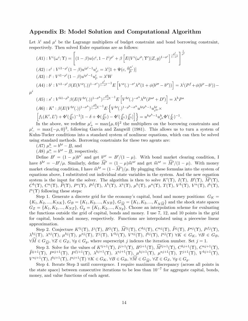
Appendix B: Model Solution and Computational Algorithm

Let λi and µi be the Lagrange multipliers of budget constraint and bond borrowing constraint,respectively. Then solved Euler equations are as follows:

(A1) : V i(ωi; Υ) =

[(1− β)u(ci, 1− li)ρi + β

[E(V i(ωi′; Υ′)|Z, g)1−σ

i] ρi

1−σi

] 1

ρi

(A2) : ci : V i1−ρi(1− β)uiρi−1ui

ci= λi[1 + Ψ(c, m̂

h′

P̂)]

(A3) : li : V i1−ρi(1− β)uiρi−1ui

li= λiW

(A4) : bi : V i1−ρiβ(E(V i′(.))1−σi)

ρi

1−σi−1E[V i′(.)−σ

iλi′(1 + φ(bi′′ − bi′))

]= λi(P f +φ(bi′−bi))−

µi

(A5) : s′ : V h1−ρhβ(E(V h′(.))1−σh)

ρh

1−σh−1E[V h′(.)−σ

hλh′(P s′ +D′)

]= λhP s

(A6) : K ′ : β(E(V h′(.))1−σh)

ρh

1−σh−1E{V h′(.)1−ρ

h−σhuh′ρh−1uh′

ch′×[

f1(K′, L′) + Φ′( I

′

K′ )−1[1− δ + Φ( I

′

K′ )− Φ′( I′

K′ )I′

K′ ]]}

= uhρh−1uh

chΦ′( IK )−1.

In the above, we redefine µi+ = max{µ, 0}2 the multipliers on the borrowing constraints andµi− = max{−µ, 0}2, following Garcia and Zangwill (1981). This allows us to turn a system ofKuhn-Tucker conditions into a standard system of nonlinear equations, which can then be solvedusing standard methods. Borrowing constraints for these two agents are:

(A7) µh− = bh′ −B, and(A8) µn− = bn′ −B, respectively.

Define B′ = (1 − µ)bn′

and get bn′ = B′/(1 − µ). With bond market clearing condition, I

have bh′ = −B′/µ. Similarly, define M̂ ′ = (1 − µ)m̂n′ and get m̂n′ = M̂ ′/(1 − µ). With money

market clearing condition, I have m̂h′ = (1− M̂ ′)/µ. By plugging these formulas into the system ofequations above, I substituted out individual state variables in the system. And the new equationsystem is the input for the solver. The algorithm is then to solve K ′(Υ), I(Υ), B′(Υ), M̂ ′(Υ),Ch(Υ), Cn(Υ), P̂ (Υ), P s(Υ), P f (Υ), λh(Υ), λn(Υ), µh(Υ), µn(Υ), T (Υ), V h(Υ), V n(Υ), lh(Υ),ln(Υ) following these steps:

Step 1. Generate a discrete grid for the economy’s capital, bond and money positions: GK ={K1,K2, ...,KNK}, GB = {K1,K2, ...,KNB}, GM̂ = {K1,K2, ...,KNM̂

} and the shock state spacesGZ = {K1,K2, ...,KNZ}, Gg = {K1,K2, ...,KNg}. Choose an interpolation scheme for evaluatingthe functions outside the grid of capital, bonds and money. I use 7, 12, and 10 points in the gridfor capital, bonds and money, respectively. Functions are interpolated using a piecewise linearapproximation.

Step 2. Conjecture K ′j(Υ), Ij(Υ), B′j(Υ), M̂ ′j(Υ), Chj(Υ), Cnj(Υ), P̂ j(Υ), P sj(Υ), P fj(Υ),λhj(Υ), λnj(Υ), µhj(Υ), µnj(Υ), T j(Υ), V hj(Υ), V nj(Υ), lhj(Υ), lnj(Υ) ∀K ∈ GK , ∀B ∈ GB,

∀M̂ ∈ GM̂

, ∀Z ∈ GZ , ∀g ∈ Gg, where superscript j indexes the iteration number. Set j = 1.

Step 3. Solve for the values of K ′j+1(Υ), Ij+1(Υ), B′j+1(Υ), M̂ ′j+1(Υ), Chj+1(Υ), Cnj+1(Υ),P̂ j+1(Υ), P sj+1(Υ), P fj+1(Υ), λhj+1(Υ), λnj+1(Υ), µhj+1(Υ), µnj+1(Υ), T j+1(Υ), V hj+1(Υ),

V nj+1(Υ), lhj+1(Υ), lnj+1(Υ) ∀K ∈ GK , ∀B ∈ GB, ∀M̂ ∈ GM̂

, ∀Z ∈ GZ , ∀g ∈ Gg.Step 4. Iterate Step 3 until convergence. I require maximum discrepancy (across all points in

the state space) between consecutive iterations to be less than 10−7 for aggregate capital, bonds,money, and value functions of each agent.

14

Appendix C: Tables and Figures

Table 1: Baseline Parameterizationparameter Value

β∗ Time discount 0.931/(1− ρh) EIS for stockholders 0.31/(1− ρn) EIS for non-stockholders 0.1µ Participation rate 0.2ρ∗z Persistence of aggregate shocks 0.95ρ∗g Persistence of aggregate money supply 0.005

θ Capital share 0.36ξ Capital adjustment cost coefficient 0.99δ∗ Depreciation rate 0.02

B Borrowing limit 6Wg∗∗ Average growth rate of money supply 1.03σε Standard deviation of technology shocks 0.015σg Standard deviation of monetary shocks 0.0045σh = σn Relative risk aversion 10/6/2χ Firm leverage 0.15

”∗” indicates that the reported value refers to the implied quarterly value for a parameter that is calibrated

to monthly frequency, while ”∗∗” indicates the implied annual value. W is the average monthly wage rate in the

economy.

Table 2: Comparison of Statistics

Asset Pricing Facts Model

RE8.11%

(19.30%)6.98%

(21.14%)

Rf1.94%

(5.44%)1.69%

(8.02%)

REP6.17%

(19.40%)5.29%

(21.55%)

Sharpe Ratio 0.32 0.25

Business Cycle Facts Model

σ(Y ) 1.89 2.71

σ(C)/σ(Y ) 0.40 0.79

σ(Ch)/σ(Y ) − 0.93

σ(Cn)/σ(Y ) − 0.72

σ(I)/σ(Y ) 2.39 2.31

σ(L)/σ(Y ) 0.80 0.26

15

Table 3: CorrelationsCorr(π,Rf ) Corr(π, if ) Corr(π,Rs) Corr(π,REP ) Corr(π, P s)

Model Statistics −0.08926 0.98911 −0.99418 −0.97979 −0.12590

Table 4: Different Money Growth Rates and Equity Premiums

Inflation (π) −1% 0% 3% 6% 9% 12%

Equity Premiums 4.95% 5.05% 5.29% 5.46% 5.54% 5.59%

Table 5: Optimal Money Growth Rates

Inflation (π) −1% 0% 3% 6% 9% 12%

Total 0.0068 0.0047 0 −0.0044 −0.0093 −0.0142

Stockholders 0.0080 0.0052 0 −0.0046 −0.0099 −0.0149

Non-Stockholers 0.0062 0.0045 0 −0.0043 −0.0091 −0.0138

1.4 1.6 1.8 2 2.2 2.4 2.6 2.84.6

4.7

4.8

4.9

5

5.1

5.2

5.3

5.4

5.5

5.6 θy=­0.05

θy=­0.025

θy=­0.01

θy=0.01

θy=0.025

θy=0.05

Benchmark

Risk­Free Returns

Equi

ty P

rem

ium

s

Figure 1: Equity premiums and Risk-free Returns under the Alternative Monetary Policy: Re-sponding to Business Cycles

16

1 1.5 2 2.54.6

4.8

5

5.2

5.4

5.6

5.8

6

Benchmark

θPE=­0.05

θPE=­0.025

θPE=­0.01

θPE=0.01

θPE=0.025

θPE=0.05

Risk­Free Returns

Equi

ty P

rem

ium

s

Figure 2: Equity premiums and Risk-free Returns under the Alternative Monetary Policy: Re-sponding to Equity Prices

17

1.5 1.55 1.6 1.65 1.7 1.75 1.8 1.85 1.9 1.95

5.1

5.15

5.2

5.25

5.3

5.35

5.4

5.45

5.5

5.55

θEP=­0.05

θEP=­0.025

θEP=­0.01

θEP=0.01

θEP=0.025

θEP=0.05

Benchmark

Risk­Free Returns

Equi

ty P

rem

ium

s

Figure 3: Equity premiums and Risk-free Returns under the Alternative Monetary Policy: Re-sponding to Equity Premiums

18

Table 6: Welfare Implications of Alternative Monetary Policies

Parameters S N Total Welare

Benchmark ρg = θEP = θPE = θy = 0 0 0 0

Panel A: To business cycles ρg = θEP = θPE = 0

Procyclical θy = 0.05 0.0040 0.0042 0.0041θy = 0.025 0.0011 0.0017 0.0015θy = 0.01 0.0003 0.0006 0.0005

Countercyclical θy = −0.01 0.0000 −0.0004 −0.0003θy = −0.025 −0.0010 −0.0016 −0.0014θy = −0.05 −0.0021 −0.0033 −0.0029

Panel B: To equity prices ρg = θEP = θy = 0

θPE = 0.05 0.0113 0.0094 0.0101θPE = 0.025 0.0034 0.0039 0.0038θPE = 0.01 0.0008 0.0013 0.0012θPE = −0.01 −0.0006 −0.0011 −0.0010θPE = −0.025 −0.0021 −0.0030 −0.0027θPE = −0.05 −0.0039 −0.0054 −0.0049

Panel C: To equity premium ρg = θPE = θy = 0

θEP = 0.10 −0.00005 0.00008 0.00004θEP = 0.075 0.00001 0.00007 0.00005θEP = 0.05 0.00008 0.00011 0.00010θEP = 0.025 0.00018 0.00019 0.00019θEP = 0.01 0.00028 0.00030 0.00029θEP = 0.00 0.00015 0.00079 0.00058θEP = −0.01 0.00019 0.00020 0.00020θEP = −0.025 0.00013 0.00012 0.00012θEP = −0.05 0.00005 0.00003 0.00004θEP = −0.075 0.00000 −0.00003 −0.00002

19

References

Pierluigi Balduzzi. Inflation and asset prices in a monetary economy. Economics Letters, 53(1):67–74, October 1996.

Ravi Bansal and II Coleman, Wilbur John. A monetary explanation of the equity premium, termpremium, and risk-free rate puzzles. Journal of Political Economy, 104(6):1135–71, December1996.

B. Barber and T Odean. Trading is hazadous to your wealth: the common stock investmentperformance of individual investors. Journal of Finance, 55:773–806, April 2000.

Brad M. Barber, Yi-Tsung Lee, Yu-Jane Liu, and Terrance Odean. Just how much do individualinvestors lose by trading? Review of Financial Studies, 22(2):609–632, February 2009.

John Beirne and Gabe de Bondt. The equity premium and inflation. Applied Financial EconomicsLetters, 4(6):439–442, 2008.

Ben S. Bernanke and Mark Gertler. Should central banks respond to movements in asset prices?American Economic Review, 91(2):253–257, May 2001.

Olivier Blanchard. Bubbles, liquidity traps, and monetary policy: Comments on jinushi et al, andon bernanke. Jan 2000.

Richard Blundell, Martin Browning, and Costas Meghir. Consumer demand and the life-cycleallocation of household expenditures. Review of Economic Studies, 61(1):57–80, January 1994.

Glenn W Boyle. Money demand and the stock market in a general equilibrium model with variablevelocity. Journal of Political Economy, 98(5):1039–53, October 1990.

W.A. Brock. Overlapping generations models with money and transactions costs. In B. M. Friedmanand F. H. Hahn, editors, Handbook of Monetary Economics, volume 1 of Handbook of MonetaryEconomics, chapter 7, pages 263–295. Elsevier, October 1990.

William A Brock. Money and growth: The case of long run perfect foresight. InternationalEconomic Review, 15(3):750–77, October 1974.

James B. Bullard and Eric Schaling. Why the fed should ignore the stock market. Review, (Mar.):35–42, 2002.

John Campbell. Estimating the equity premium. Scholarly Articles 3196339, Harvard UniversityDepartment of Economics, 2008.

John Y. Campbell and Tuomo Vuolteenaho. Inflation illusion and stock prices. NBER WorkingPaper No. 10263, Jan 2004.

Otaviano Canuto. The arrival of asset prices in monetary policy. October 2009.

Stephen G. Cecchetti. Understanding the great depression: Lessons for current policy. NBERWorking Papers 6015, National Bureau of Economic Research, Inc, April 1997.

Lawrence Christiano, Cosmin L. Ilut, Roberto Motto, and Massimo Rostagno. Monetary policyand stock market booms. NBER Working Papers 16402, National Bureau of Economic Research,Inc, September 2010.

20

James Claus. Equity premia as low as three percent? evidence from analysts’ earnings forecasts fordomestic and international stock markets. Journal of Finance, 56(5):1629–1666, October 2001.

John H Cochrane. Production-based asset pricing and the link between stock returns and economicfluctuations. Journal of Finance, 46(1):209–37, March 1991.

Jean-Pierre Danthine and John B. Donaldson. Inflation and asset prices in an exchange economy.Econometrica, 54(3):585–605, May 1986.

Jean-Pierre Danthine and John B Donaldson. Labour relations and asset returns. Review ofEconomic Studies, 69(1):41–64, January 2002.

Larry G Epstein and Stanley E Zin. Substitution, risk aversion, and the temporal behavior ofconsumption and asset returns: A theoretical framework. Econometrica, 57(4):937–69, July1989.

Robert C. Feenstra. Functional equivalence between liquidity costs and the utility of money. Journalof Monetary Economics, 17(2):271–291, 1986.

Michael F. Gallmeyer, Burton Hollifield, Francisco J. Palomino, and Stanley E. Zin. Arbitrage-freebond pricing with dynamic macroeconomic models. Review, (Jul):305–326, 2007.

Athanasios Geromichalos, Juan M Licari, and Jose Suarez-Lledo. Monetary policy and asset prices.Review of Economic Dynamics, 10(4):761–779, October 2007.

Giovannini and Labadie. Asset prices and interest rates in cash-in-advance models. JPE, 1991.

Jeremy Greenwood, Zvi Hercowitz, and Gregory W Huffman. Investment, capacity utilization, andthe real business cycle. American Economic Review, 78(3):402–17, June 1988.

Christopher Gust and David Lopez-Salido. Monetary policy and the cyclicality of risk. InternationalFinance Discussion Papers 999, Board of Governors of the Federal Reserve System (U.S.), 2010.

Fatih Guvenen. Reconciling conflicting evidence on the elasticity of intertemporal substitution: Amacroeconomic perspective. Journal of Monetary Economics, 53(7):1451–1472, October 2006.

Fatih Guvenen. A parsimonious macroeconomic model for asset pricing. Econometrica, 77(6):1711–1750, November 2009.

Robert J Hodrick, Narayana R Kocherlakota, and Deborah Lucas. The variability of velocity incash-in-advance models. Journal of Political Economy, 99(2):358–84, April 1991.

David Humphrey, Magnus Willesson, Goran Bergendahl, and Ted Lindblom. Cost savings fromelectronic payments and atms in europe. Working Papers 03-16, Federal Reserve Bank of Philadel-phia, 2003.

Peter N. Ireland. On the welfare cost of inflation and the recent behavior of money demand.American Economic Review, 99(3):1040–52, June 2009.

Otmar Issing. Asset prices and monetary policy. The Cato Journal, Winter, 2009.

Ravi Jagannathan, Ellen R. McGrattan, and Anna Scherbina. The declining u.s. equity premium.Quarterly Review, (Fall):3–19, 2000.

21

Henry Kim, Jinill Kim, and Robert Kollmann. Applying perturbation methods to incompletemarket models with exogenous borrowing constraints. Discussion Papers Series, Department ofEconomics, Tufts University 0504, Department of Economics, Tufts University, 2005.

Miles S. Kimball and Matthew D. Shapiro. Social security, retirement and wealth: Theory andimplications. Working Papers wp054, University of Michigan, Michigan Retirement ResearchCenter, June 2003.

Nobuhiro Kiyotaki and Randall Wright. On money as a medium of exchange. Journal of PoliticalEconomy, 97(4):927–54, August 1989.

Donald L. Kohn. John taylor rules. October 2007.

Per Krusell and Anthony A. Smith. Income and wealth heterogeneity, portfolio choice, and equi-librium asset returns. Macroeconomic Dynamics, 1(02):387–422, June 1997.

Kyriacos Kyriacou, Jakob B. Madsen, and Bryan Mase. Does inflation exaggerate the equitypremium? Journal of Economic Studies, 33(5):344–356, November 2006.

Pamela Labadie. Stochastic inflation and the equity premium. Journal of Monetary Economics,24(2):277–298, September 1989.

Martin Lettau, Sydney C. Ludvigson, and Jessica A. Wachter. The declining equity premium:What role does macroeconomic risk play? Review of Financial Studies, 21(4):1653–1687, July2008.

David A. Marshall. Inflation and asset returns in a monetary economy. The Journal of Finance,47(4):1315–1342, 1992.

Frederic S. Mishkin. Financial stability and the macroeconomy. Economics wp09, Department ofEconomics, Central bank of Iceland, May 2000.

Waller Nosal and Wright. Introduction to the macroeconomic dynamics: Special issues onmoney,credit, and liquidity. 2010.

Francisco Palomino. Monetary policy, time-varying risk premiums, and the. economic content ofbond yields. Aug 2010.

Bianca De Paoli and Pawel Zabczyk. Cyclical risk aversion, precautionary saving and monetarypolicy. March 2012.

Jay R. Ritter and Richard S. Warr. The decline of inflation and the bull market of 19821999.Journal of Financial and Quantitative Analysis, 37(01):29–61, March 2002.

Jr. Robert E. Lucas. Inflation and welfare. Econometrica, 68(2):247–274, March 2000.

Glenn D. Rudebusch, Brian P. Sack, and Eric T. Swanson. Macroeconomic implications of changesin the term premium. Review, (Jul):241–270, 2007.

Stephanie Schmitt-Grohe and Martin Uribe. Optimal fiscal and monetary policy under stickyprices. Journal of Economic Theory, 114(2):198–230, February 2004.

Maral Shamloo and Aytek Malkhozov. Asset prices in affine real business cycle models. IMFWorking Papers 10/249, International Monetary Fund, November 2010.

22

Jeremy J . Siegel. The shrinking equity premium. The Journal of Portfolio Management, 26(1):10–17, 1999.

Kjetil Storesletten, Chris Telmer, and Amir Yaron. Asset pricing with idiosyncratic risk andoverlapping generations. Review of Economic Dynamics, 10(4):519–548, October 2007.

Thomas D. Tallarini. Risk-sensitive real business cycles. Journal of Monetary Economics, 45(3):507–532, June 2000.

John Tatom. Inflation and asset prices. MPRA Paper 34606, University Library of Munich,Germany, November 2011.

Ping Wang and Chong K Yip. Alternative approaches to money and growth. Journal of Money,Credit and Banking, 24(4):553–62, November 1992.

Philippe Weil. Nonexpected utility in macroeconomics. The Quarterly Journal of Economics, 105(1):29–42, February 1990.

23