NBER WORKING PAPER SERIES

MONETARY DISCRETION, PRICING COMPLEMENTARITYAND DYNAMIC MULTIPLE EQUILIBRIA

Robert G. KingAlexander L. Wolman

Working Paper 9929http://www.nber.org/papers/w9929

NATIONAL BUREAU OF ECONOMIC RESEARCH1050 Massachusetts Avenue

Cambridge, MA 02138August 2003

This paper is an outgrowth of the authors’ work in progress with Aubhik Khan, available athttp://www.rich.frb.org/pubs/wpapers/pdfs/wp01-8.pdf; it does not necessarily represent the views of theFederal Reserve System, the Federal Reserve Board, or the Federal Reserve Bank of Richmond. We havebenefited from conversations with Russell Cooper, Huberto Ennis, Andreas Hornstein, John Leahy and HenrySiu, and from presentations at Harvard, Iowa, MIT, the New York Fed, UQAM, Western Ontario, Wharton,York, and the conference on Dynamic Models at the Bank of Canada, July 2003. The views expressed hereinare those of the authors and not necessarily those of the National Bureau of Economic Research.

©2003 by Robert G. King and Alexander L. Wolman. All rights reserved. Short sections of text, not toexceed two paragraphs, may be quoted without explicit permission provided that full credit, including ©notice, is given to the source.

Monetary Discretion, Pricing Complementarity and Dynamic Multiple EquilibriaRobert G. King and Alexander L. WolmanNBER Working Paper No. 9929August 2003JEL No. E5, E61, D78

ABSTRACT

In a plain-vanilla New Keynesian model with two-period staggered price-setting, discretionarymonetary policy leads to multiple equilibria. Complementarity between the pricing decisions offorward-looking firms underlies the multiplicity, which is intrinsically dynamic in nature. At eachpoint in time, the discretionary monetary authority optimally accommodates the level ofpredetermined prices when setting the money supply because it is concerned solely about realactivity. Hence, if other firms set a high price in the current period, an individual firm will optimallychoose a high price because it knows that the monetary authority next period will accommodate witha high money supply. Under commitment, the mechanism generating complementarity is absent: themonetary authority commits not to respond to future predetermined prices.

We compute a traditional inflation bias equilibrium, in which price-setters are optimistic, rationallyexpecting small adjustments by other firms. But there is another steady-state equilibrium in whichprice setters are pessimistic and inflation is much higher. Further, we find that there are multipleequilibria at a point in time, not just in steady states. In a stochastic setting with equilibriumselection each period determined by an i.i.d. sunspot, there is greater inflation bias on average thanif price-setters were always optimistic. The sunspot realization also has real effects: periods ofhigher than average inflation are accompanied by low output. Thus, increased real volatility may bean additional cost of discretion in monetary policy.

Robert G. King Alexander L. WolmanDepartment of Economics Research DepartmentBoston University Federal Reserve Bank of Richmond270 Bay State Road 701 East Byrd StreetBoston, MA 02215 Richmond, VA 23219and NBER Alexander.Wolman@rich.frb.orgrking@bu.edu

1 IntroductionIn the debate over rules versus discretion for monetary policy, the primary argumentagainst discretion has been that it leads to a higher average inflation than is optimalwith commitment. In the consensus basic model which has developed following Kyd-land and Prescott [1977] and Barro and Gordon [1983], the discretionary monetaryauthority seeks to produce unexpected inflation to stimulate real output, which is in-efficiently low because of distortions in the economy. But since it cannot fool agentsin rational expectations equilibrium, the discretionary monetary authority producesexpected inflation that has a negligible real effect on output, while imposing othercosts on the economy.By contrast, this paper provides an example of a different, potentially adverse,

consequence of discretionary monetary policy: it can lead to multiple equilibria and,thus, to the possibility of endogenous fluctuations in inflation and real activity thatare not related to the economy’s fundamentals. We illustrate this possibility within asimple dynamic macroeconomic model that has important New Keynesian features:(i) monopolistic competition, making output inefficiently low; and (ii) a staggeredpricing structure in which firms set nominal prices that must be held fixed for twoperiods. These two features give the monetary authority some leverage over realactivity.In this simple setting, the multiplicity of equilibria derives from interaction be-

tween two features of the economy. First, firms adopt forward-looking pricing rulesbecause their nominal prices are held fixed for two periods. In choosing a price, firmsin the current period need to form expectations about the behavior of the monetaryauthority — and firms — in the next period. A higher future money supply leads toa higher future nominal marginal cost, which raises the optimal price for a firm inthe current period. Second, under discretion, the monetary authority takes as givenprices set in previous periods in determining its choice of the money stock in eachperiod. Since its concern is to maximize the welfare of the representative agent, whichdepends on real variables, it chooses a money stock that is proportional to the priceset by firms in the previous period, which we call a homogenous money stock rule.The combination of forward-looking pricing with discretionary policy leads to

complementarity between the price-setting actions of firms: if all other firms set ahigher price in the current period, the monetary authority will set a higher moneysupply in the subsequent period, raising the desired price for a single firm in thecurrent period.We show that this policy-induced complementarity implies that there are typically

two private-sector equilibria which can prevail at any point in time and two steady-state equilibria. In general, there is one equilibrium in which firms expect smalladjustments and the newly set price is relatively close to the price that firms setlast period. But there is another in which the adjusting firms make a much largeradjustment.

2

Because this multiplicity of equilibria arises for arbitrary homogenous monetarypolicies, it also arises with an optimizing monetary authority who cannot committo future actions. We begin by considering settings of perfect foresight, in whichthe monetary authority and private agents each assume that only one of the twotypes of private sector equilibria will occur. We show that there are two steady-state discretionary equilibria, one with low inflation bias and one with high inflationbias. It is notable that the complementarity which generates multiple equilibria isentirely due, in our model, to the nature of monetary policy under discretion. Thatis: our specification of preferences and the labor market is such that there is nocomplementarity in the price-setting behavior of firms if the central bank maintainsa fixed nominal money stock. Our setup thus highlights the role of discretionarymonetary policy in generating complementarity.There are three components of the existing literature to which our paper relates.

First, there is the voluminous literature on monetary policy under discretion, whichbegins with Kydland and Prescott [1977] and Barro and Gordon [1983]. In that lit-erature, output is inefficiently low, but can be raised by policies that also produceunexpected inflation. There are costs of actual inflation, so that a consistent equi-librium exhibits an inflation bias. The model that captures these ideas involves aquadratic monetary authority objective and a linear economic model. There is aunique discretionary equilibrium in the standard model (absent reputational effectsor trigger strategies).Second, there is an important recent literature that works out how the standard

KPBG model can be derived from a fully articulated New Keynesian framework. Thekey ingredients of the models in this literature are that output is inefficiently low dueto monopoly distortions; the monetary authority has temporary leverage over thereal economy because of staggered price setting; and the costs of actual inflation arewelfare losses associated with relative price distortions. In these settings, just as inthe KPBG model, there is an inflation bias under discretion.1 However, this analysishas been conducted within linearized versions of modern sticky price models.Our analysis takes the most basic fully articulated New Keynesian model, without

linearizing, and shows that there are multiple equilibria. Our model features costsof stimulative policies — which bring about actual inflation — that stem from relativeprice distortions across goods. It also features benefits from unexpected stimulativepolicies, which lower monopoly markups and raise output toward the first best level.Our model is an explicitly dynamic one, with firms forecasting future inflation whensetting nominal prices for two periods. As we have stressed above, multiple equilibriacan occur in our model due to complementarity mechanisms similar to those stressedin the literature on coordination failures. The possibility of such responses is excludedby a model that is linear.

1For a textbook treatment, see the derivation in Woodford [2002, chapter 3]. The inflationbias result under discretion within such optimizing New Keynesian models has been popularized byClarida, Gali and Gertler [1999].

3

Third, our paper is closely related to recent work by Albanesi, Chari and Chris-tiano [2002]. They find multiple equilibria in an essentially static model where aportion of monopolistically competitive firms must set prices before the monetaryauthority’s action in each period. At the same time, the structure of the model theystudy is quite different from ours. The stimulative policies that produce inflation intheir model also raise nominal interest rates and lead to money demand distortions,either by driving a relative price wedge between the cost of buying goods on cashand credit or by increasing transactions time. A monetary authority thus faces atrade-off between the benefits of driving down the markup and these costs. In ourmodel, instead of the costs of realized inflation being related to money demand, theyinvolve price distortions across goods whose prices were set in different periods.If there are sunspots which switch the economy between equilibria, there are also

important differences in the consequences that are suggested by our model from thosesuggested by the ACC models. In our setting, if a high inflation equilibrium occurswhen agents attach low probability to such an event, then there will be a declinein output because aggregate demand will fall and the average markup will increase.By contrast, in the ACC models, a switch from low inflation to high inflation willhave little effect on the average markup or output, with the main difference beingthe extent of money demand distortions. Since the ACC models are essentially staticones, there is also another difference: there is no feedback between the likelihood thateconomic agents attach to future equilibria and the levels of inflation and output ata point in time. Accordingly beliefs about the future are of no bearing for currentevents. In our model, beliefs about future outcomes affect the nature of the currentpolicy problem because firms setting their price in the current period care about bothcurrent and future monetary policy.

2 ModelThe model economy that we study is a particular fully articulated “New Keynesian”framework, featuring monopolistic competition and nominal prices which are fixedfor two periods. There is staggered pricing, with one-half of a continuum of firmsadjusting price in each period. Since all of the firms have the same technology andface the same demand conditions, it is natural to think of all adjusting firms aschoosing the same price. We impose this symmetry condition in our analysis.There are many different types of New Keynesian models, which differ in terms of

their implications for the extent of complementarity in price-setting. Our particularmodel assumes that (i) there is a constant elasticity demand structure originatingfrom a Dixit-Stiglitz aggregator of differentiated products; (ii) there is a centralizedlabor market so that the common marginal cost for all firms is powerfully affected byaggregate demand; and (iii) preferences for goods and leisure display exactly offsettingincome and substitution effects of wage changes, as is common in the literature onreal business cycles. Kimball [1995] and Woodford [2002] have stressed that these

4

assumptions make it difficult to generate complementarity between price-setters whenthere is an exogenous money stock. As we will, see our model has exactly zerocomplementarity in this situation. From our perspective, this is a virtue becauseit highlights the importance of the policy-based complementarity that arises frommonetary policy under discretion.2

2.1 Households

There is a representative household, which values consumption (ct) and leisure (lt)according to a standard time separable expected utility objective,

Et{∞Xj=0

βju(ct+j, lt+j)} (1)

with β being the discount factor which is taken to be close to one. We assume thatthe momentary utility function takes the form

u(ct, lt) = log(ct) + χlt (2)

which implies that there are exactly off-setting income and substitution effects ofwage changes. It also has some other convenient implications that we describe later.As is standard in the analyses of imperfect competition macro models that follow

Blanchard and Kiyotaki [1987] and Rotemberg [1987], we assume that consumptionis an aggregate of a continuum of individual goods, ct = [

R 10ct(z)

(ε−1)/εdz]ε/(ε−1).Households distribute their expenditure efficiently across these goods, resulting inconstant-elasticity demands for individual products from each of the two types offirms which they will encounter in the equilibrium below:

cj,t =

µPj,tPt

¶−εct, j = 0, 1. (3)

The subscript j in (3) denotes the age of the nominal price, so that P0,t is the priceset by firms in period t and P1,t is the price set by firms one period previously (P1,t = P0,t−1). Likewise, cj,t is the period-t demand for goods produced by a firm thatset its price in period t− j. The price level which enters in these demands takes theform

Pt = [1

2P 1−ε0,t +

1

2P 1−ε1,t ]

11−ε . (4)

We assume that households also hold money to finance expenditure according to

Mt =

Z 1

0

Pt(z)ct (z) dz (5)

2Glomm and Ravikumar [1995] show how endogenous government policy of a different sort —public education — can generate multiple equilbria.

5

so that our model imposes a constant, unit velocity, in common with many macro-economic analyses.3 We adopt this specification because it allows us to abstractfrom all the wealth and substitution effects that normally arise in optimizing mod-els of money demand, so as to focus on the consequences of price-stickiness. Withconstant-elasticity demands for each good, the money-demand specification in (5)implies

Mt = Ptct. (6)

Since this is a representative agent model and since no real accumulation is possiblegiven the technologies described below, we are not too explicit about the consumption-saving aspect of the household’s problem; it will be largely irrelevant in general equi-librium except for asset-pricing. We simply assume that there is a Lagrange multiplierthat takes the form

λt =∂u(ct, lt)

∂ct=1

ct, (7)

and that households equate the marginal rate of substitution between leisure andconsumption to the real wage rate prevailing in the competitive labor market, i.e.,

wt =∂u(ct, lt)/∂lt∂u(ct, lt)/∂ct

= χct. (8)

In each case, the second equality indicates the implications of the specific utilityfunction introduced above.

2.2 Firms

Firms produce output according to a linear technology, where for convenience weset the marginal product of labor to one. So, for each type of firm, the productionfunction is

cj,t = nj,t. (9)

This implies that real marginal cost is unrelated to the scale of the firm or its typeand is simply

ψt = wt

and that nominal marginal cost is Ψt = Ptψt = PtwtMuch of our analysis will focus on the implications of efficient price-setting by the

monopolistically competitive firm. The adjusting firms in period t are assumed toset prices so as to maximize the expected present discounted value of their revenues,using the household’s marginal utility as a (possibly stochastic) discount factor. Thatis, they choose P0,t to maximize their market value,

3We think of this quantity equation as the limiting version of a standard money demand functionwhich occurs as the own return on money is raised toward the nominal interest rate (see King andWolman [1999] for some additional discussion).

6

[λt(P0,t −Ψt)c0,t + βEtλt+1PtPt+1

(P0,t −Ψt+1)c1,t+1].

As monopolistic competitors, firms understand that c0,t = (P0,tPt)−εct and that c1,t+1 =

( P0,tPt+1

)−εct+1, but take ct, Pt, ct+1 and Pt+1 as not affected by their pricing decisions.The efficient price must accordingly satisfy

P0,t =ε

ε− 1P ε−1t Ψt + βEt

¡P ε−1t+1 Ψt+1

¢P ε−1t + βEt

¡P ε−1t+1

¢ , (10)

where we again give the result under the specific momentary utility function. In fact,this reveals one motivation for the form of the particular utility function chosen. Ingeneral, both aggregate demand (ct) and the discount factor (λt) affect the weights,but our choice of a utility function that is logarithmic in consumption means thatthese two effects exactly cancel out. With perfect foresight, the pricing equation canbe written compactly as

P0,t =ε

ε− 1[(1− θt,t+1)Ψt + θt,t+1Ψt+1]; (11)

the optimal price is a constant markup (ε/ (ε− 1)) over a weighted average of nominalmarginal cost over the two periods, where the weight on the future is

θt,t+1 =βλt+1ct+1P

ε−1t+1

λtctPε−1t + βλt+1ct+1P

ε−1t+1

=βP ε−1

t+1

P ε−1t + βP ε−1

t+1

. (12)

The weights on current and future nominal marginal cost represent the shares ofmarginal revenue associated with the current and future periods.

2.3 Defining Complementarity in Price Setting

The standard definition of complementarity — contained, for example, in Cooper andJohn [1988]— is that the optimal action of one decision-maker is increasing in theactions of other similar decision-makers. In our context, we are interested in com-plementarity in price-setting in equation (11). The left-hand side of this expressionis the action of the particular decision-maker under study: the optimal price of anindividual monopolistically competitive firm that is currently making a price adjust-ment. Other monopolistically competitive firms are also simultaneously adjustingprices: these firms take an action P0,t that influences the right-hand of (11). Theprice chosen by the representative adjusting firm influences the price level directlybecause Pt = [12P

1−ε0,t +

12P 1−ε1,t ]

11−ε and may also affect current nominal marginal cost.

Given that prices are sticky, there can be real effects of variations in the price level, sothat these could influence nominal marginal cost. Finally, the weights on the presentand the future in (11) also depend on the price level. To determine whether there is

7

complementarity, we must work through these mechanisms and determine the signof the relevant partial derivative. The extent of complementarity will depend on thebehavior of the monetary authority.

2.4 Timing

The sequence of actions within a period is as follows. In the first stage, the monetaryauthority chooses the money stock, Mt, taking as given P1,t, the price set by firms inthe previous period. In the second stage, adjusting firms set prices (P0,t). Simulta-neously, wages are determined and exchange occurs in labor and goods markets.There are two important consequences of these timing assumptions. First, since

price-setters move after the monetary authority, they cannot be surprised by themonetary authority during the initial period that their price is in effect. Accordingly,the monetary authority faces an economy in which it can surprise some agents (thosewith pre-set prices) but not others (those adjusting prices) within a period. Thisgives rise to a relative price distortion across firms in the discretionary equilibriumthat we construct, which in turn means that there is an interior solution for themonetary authority’s choice problem. If we reversed the timing order so that themonetary authority moved last, we conjecture that there would not be a discretionaryequilibrium unless some other aspect of the economy were modified, such as allowingfirms to reset their prices after paying an adjustment cost.4 Second, the fact that theprice-setters move after the monetary authority means that there is the potential formore than one equilibrium price to correspond to a given monetary policy action.

2.5 Complementarity with an exogenous money stock

We now consider a situation in which Mt = Mt+1 = M . Under the assumptions ofour model, it turns out to be easy to investigate the influence of other adjusting firm’sactions, i.e., to compute the effect of P0,t on the right-hand side of (11). With theconstant velocity assumption (Ptct = Mt) and with the particular utility function,Ψt = Ptwt = Pt(χct). Hence, equilibrium nominal marginal cost is exactly propor-tional to the money stock, Ψt = χMt. Since the nominal money stock is assumedconstant over time, nominal marginal cost is also constant over time and (11) becomes

P0,t =ε

ε− 1χM.

This equilibrium relationship means that there is an exactly zero effect of P0,t on theright-hand side: there is no complementarity in price-setting in this model when thenominal money supply is constant.

4The nonexistence of a discretionary equilibrium is a feature of Ireland’s [1997] analysis of amodel in which all prices are set simultaneously, before the monetary authority determines thecurrent money supply.

8

2.6 Summarizing the economy by p0 and m

Under discretionary policy, the monetary authority will not choose to keep the nom-inal money supply constant. Therefore, the optimal pricing condition (11) will notsimplify to a static equation. In general, however, equilibrium will be a function ofjust two variables: a measure of the price set by adjusting firms and a measure ofmonetary policy. We construct these variables by normalizing nominal prices andmoney by the single nominal state variable in this economy, the price set by firms inthe previous period (P1,t = P0,t−1). Define the normalized money supply as

mt =Mt/P1,t, (13)

and the normalized price set by adjusting firms in the current period as

p0,t = P0,t/P1,t. (14)

We can then express all variables of interest as functions of these two normalizedvariables. From (4), the normalized price level is a function of only p0,t :

PtP1,t

= g(p0,t),

whereg(p0,t) ≡ [1

2p1−ε0,t +

1

2]

11−ε .

Aggregate demand is a function of both p0,t and mt :

ct = c(p0,t,mt) ≡ mt

g(p0,t).

This follows from the money demand equation:

ct =Mt

Pt=Mt

P1,t

P1,tPt

=mt

g(p0,t).

Further, since nt = [12n0,t+12n1,t] = [

12c0,t+

12c1,t], we can use the individual demands

together to show that total labor input is also pinned down by p0,t and mt :

nt = n(p0,t,mt) ≡ 12· c(p0,t,mt) · [g (p0,t)]ε ·

¡p−ε0,t + 1

¢.

Leisure is the difference between the time endowment and labor input. Marginal costis

ψt = wt =∂u(ct, lt)/∂lt∂u(ct, lt)/∂ct

= χct = ψ(mt, p0,t).

9

Another variable of interest is the gross inflation rate, Pt+1/Pt. It is determined bycurrent and future p0:

Pt+1Pt

= π(p0,t, p0,t+1) ≡ g(p0,t+1)g(p0,t)

p0,t. (15)

This follows directly fromwriting the inflation rate as a a ratio of normalized variables:

Pt+1Pt

=Pt+1/P0,tPt/P1,t

P0,tP1,t

=g(p0,t+1)

g(p0,t)p0,t.

In a steady state, there is thus a simple relationship between inflation and the relativeprice, π = p0.

2.7 Two distortions and monetary policy

The monetary authority in this model faces two distortions that are present in theprivate economy and can be influenced by its actions. First, there is a markup distor-tion that represents the wedge between price and marginal cost: it has consequencessimilar to those of a tax on labor income. The extent of this average markup is justthe reciprocal of real marginal cost,

µt =1

ψt=1

wt=

∂u(ct, lt)/∂ct∂u(ct, lt)/∂lt

=1

χct.

From the derivations above, the markup depends on p0,t and mt: µt = g(p0,t)/(χmt).Second, there is a relative price distortion that represents a wedge between inputsand outputs:

nt/ct = δ(p0,t) ≡ 12· [g (p0,t)]ε ·

¡p−ε0,t + 1

¢.

The relative price distortion depends solely on p0,t. It takes on a value of unity atp0,t = 1 (this would be the case in a zero inflation steady state) and is higher for othervalues of p0,t. The trade-off that the monetary authority typically faces between thesetwo distortions is that choosing a higher money supply decreases the markup (good)and raises the relative price distortion (bad).Just as we showed above that all real variables could be described in terms of p0

and m, the distortions can be described similarly. The summary role of p0 and m,together with the fact that at any point in time the monetary authority can choosem (i.e. choosing m in the current period is no different than choosing M) has astrong implication for the analysis of discretionary monetary policy.5 It implies thatthe level of the predetermined nominal price P1,t does not restrict the outcomes a

5It is important not to misinterpret the parenthetical statement: any choice of Mt can be repli-cated by choosing mt = Mt/P1,t. However, a policy of keeping Mt constant is not the same as apolicy of keeping mt constant.

10

discretionary policymaker can achieve, as long as the monetary authority in futureperiods behaves in the same manner.6

We now analyze outcomes under monetary discretion, proceeding in three steps(with each a separate section of the paper). We begin by studying perfect foresightsettings. In section 3, we detail the nature of perfect foresight private sector equilibriaunder a particular class of monetary policy rules. In section 4, we describe a fulldiscretionary equilibrium — with optimization by the monetary authority–in whichpolicy is shown to be in this class of rules. Finally, in section 5, we discuss stochasticequilibria, with an optimizing private sector and monetary authority.

3 Equilibrium with homogeneous policy

We begin by studying the nature of equilibrium price-setting (p0,t) given an arbitraryaction by the monetary authority and given perfect foresight. We assume that themonetary authority adopts a policy rule of the form

Mt = mtP0,t−1, (16)

where mt is viewed as the policy variable. That is, the money supply is proportionalto the prices that adjusting firms set one period ago with a constant of proportionalitymt. We call this a homogenous monetary policy rule. This form of monetary accom-modation of past nominal variables is characteristic of optimal monetary policy underdiscretion, for the following reason. The monetary authority is concerned about thereal variables that enter in private agents’ utility. It takes past prices as given, andthere is no mechanism by which the level of nominal predetermined prices necessar-ily constrains the behavior of a discretionary policymaker.7 Thus, if we viewed Minstead of m as the policy instrument, we would find that the optimizing monetaryauthority adjusted Mt proportionally to P1,t, just as is specified in (16). It will econ-omize slightly on notation and computation to viewmt as the policy instrument, andthere is no loss in generality. In a discretionary equilibrium, mt will be chosen tomaximize welfare; in this section mt is arbitrary.8

A homogenous money supply rule means that future monetary policy depends onthe price set by adjusting firms today,

Mt+1 = mt+1P0,t.

6If the future monetary authority paid attention to nominal levels, it might be optimal for thecurrent monetary authority to do the same. We do not consider equilibria with this property.

7The word “necessarily” appears because one could construct non-Markov equilibria in whichall agents agreed that P1,t did constrain the monetary authority. See previous footnote. We do notstudy such equilibria.

8By contrast, under commitment, the monetary authority commits not to respond to P1,t, andthe choice is over sequences ofMt. King and Wolman (1999) study optimal policy with commitmentin the model used here.

11

Consequently, under homogeneous policy and using the preferences introduced above,it follows from the efficient price-setting condition (11) that the nominal price set byadjusting firms (P0,t) satisfies

P0,t =εχ

ε− 1 ((1− θt,t+1)mtP1,t + θt,t+1mt+1P0,t) (17)

in equilibrium. The derivation of (17) from (11) involves (i) using the fact that nom-inal marginal cost is Ψt = Ptχct given the specific utility assumption; (ii) imposingmonetary equilibrium (Mt = Ptct); and (iii) imposing the homogenous form of themonetary policy rule (Mt = mtP1,t). From (17), the normalized price set by adjustingfirms (p0,t) satisfies

p0,t =

µεχ

ε− 1¶((1− θt,t+1)mt + θt,t+1mt+1p0,t) (18)

≡ r(p0,t,mt, p0,t+1,mt+1).

The weight on future nominal marginal cost, which was defined in (12), can be writtenin terms of current and future normalized prices as

θ(p0,t, p0,t+1) =βπ(p0,t, p0,t+1)

ε−1

1 + βπ(p0,t, p0,t+1)ε−1. (19)

where we are now explicit about how θt,t+1 depends on the present and the future.Equation (18) is a nonlinear difference equation in p0 and m that must be satisfiedin a perfect foresight equilibrium with homogeneous policy.We view p0,t on the left-hand side of (18) as describing what an individual firm

finds optimal given the actions of other price-setters and the monetary authority. Onthe right hand side, p0,t then represents all other adjusting firms’ pricing behavior,and the function on the right hand side represents the implications of those firms’behavior for the marginal revenues and costs of an individual firm. In other words,r(.) is a best-response function for the individual firm. We restrict attention to sym-metric equilibria, so that prices chosen by all adjusting firms are identical. We definecomplementarity in terms of a positive partial derivative of the response function withrespect to its first argument. That is: with perfect foresight, there is complementarityif ∂r(p0,t,mt, p0,t+1,mt+1)/∂p0,t > 0.In sections 3.2 and 3.3 below, we will make intensive use of the perfect-foresight

best-response function (18). First, we will use it to describe point-in-time equilibria;this involves characterizing the fixed points for p0,t, taking as given mt,mt+1, andp0,t+1. Second, we will use it to determine the model’s steady-state equilibria underconstant arbitrary policy. That is, we will impose p0,t = p0,t+1 and mt = mt+1 = mand determine the equilibrium value(s) (fixed points) for p0. Both of these exerciseswill then serve as inputs to our analysis of discretionary equilibria. There, (18) willsummarize private sector equilibrium for any action that the monetary authority

12

contemplates, under perfect foresight.9 With uncertainty, (18) will not hold exactly,but the mechanisms discussed here will still be relevant.

3.1 Complementarity under homogeneous monetary policy

There are two mechanisms for complementarity in (17) and (18) that will be operativein our analysis of both point-in-time and steady-state equilibria. First, holding fixedthe weights, P0,t has a positive effect on the right-hand side in (17): it enters linearlywith a coefficient of

¡εχε−1¢θt,t+1mt+1, which is positive because firms are forward-

looking and the monetary authority raises nominal Mt+1 proportionately with P0,t.Hence the specification of monetary policy has introduced some complementarity intoan economy in which it was previously absent.Second, the weights in these expressions vary with the current price P0,t (or its

normalized counter part p0,t). This additional channel plays an important role in ouranalysis. A reference value for the weight θt,t+1 is one-half, since (12) implies that theweight is β/(1+β) with β close to one if if Pt = Pt+1. An upper bound on this weightis one: this is a situation where firms place full weight on the future. Increases inthe weight raise the extent of the effect discussed above, i.e., they raise the coefficient¡

εχε−1¢θt,t+1mt+1 that measures the extent of complementarity. The second mechanism

is then that an increase in P0,t (or its normalized counterpart p0,t) raises the weight onthe future. This occurs because a firm’s profits are not symmetric around its optimalprice. As the firm’s relative price rises, its profits decline gradually, asymptoticallyreaching zero as the price goes to infinity. By contrast, as the price falls, the firmsprofits decline sharply toward zero and may even become highly negative if the firmis not allowed to shut down its operations.10 Thus, when P0,t increases for all otherfirms, future monetary accommodation — and the associated higher nominal price setby firms in the future — automatically lower’s the firm’s future relative price. Thecostliness of a low relative price leads the firm to put increased weight on futuremarginal cost.

3.2 Equilibrium analysis of steady states

To characterize steady-state equilibria for arbitrary constant, homogeneous monetarypolicies, we impose constant m and p0 on the right hand side of (18). Steady-stateequilibria are fixed points of the resulting steady-state best-response function for p0:

p0 =εχ

ε− 1m[1− θ(p0, p0) + θ(p0, p0)p0], (20)

9If we impose mt = mt+1 but allow p0t to differ from p0,t+1, then (18) describes the dynamicsof p0,t for constant homogeneous policy. Such analysis might reveal interesting dynamics. However,it is not an input into our analysis of discretionary equilibrium.

10At this point in the analysis, we do not explicitly take into account the shut-down possibility.But, when we calculate discretionary equilibria, we do verify that the equilibria are robust to allowingfirms to shut down.

13

with a weight on the future of

θ(p0, p0) =βpε−10

1 + βpε−10

. (21)

Fixed points of the steady-state best-response function are constructed by simulta-neously varying current and future p0 on the right hand side. This is in contrast tofixed points of the basic point-in-time best-response function, which are constructedholding fixed p0,t+1.

3.2.1 Uniqueness occurs at zero inflation

A zero inflation steady state involves p0 = 1. Such a steady state exists when thenormalized quantity of money is m∗ ≡ ( ε

ε−1χ)−1. In this case, the weight on the

future is θ = β/(1 + β), which is roughly one-half. The zero-inflation steady state isasymptotically optimal under full commitment in this model (see King and Wolman[1999]) and provides an important benchmark. Furthermore, ifm = m∗, zero inflationis the unique steady state; that is, p0 = 1 is the unique solution to (20) whenm = m∗.

3.2.2 Multiplicity or nonexistence must occur with positive inflation

We refer to any m > m∗ as an inflationary monetary policy, because if inflation ispositive in a steady state, then m > m∗, as we now show. From (20), given thatπ = p0 in steady state, we have

m =1

( εε−1χ)

π

[1− θ + θπ]=

1

[θ + (1− θ) ( 1π)]m∗.

Thus, π > 1 if and only if m > m∗.Proposition 1 states that under an arbitrary inflationary monetary policy, for low

values of m there are two steady-state equilibrium values of p0. For high values of m,no steady-state equilibrium exists. In a knife edge case there is a unique steady-stateequilibrium.

Proposition 1 There exists an em > m∗ such that for m ∈ (m∗, em) there are twosteady-state equilibria, and for m > em there is no steady-state equilibrium.

Proof. see Appendix.

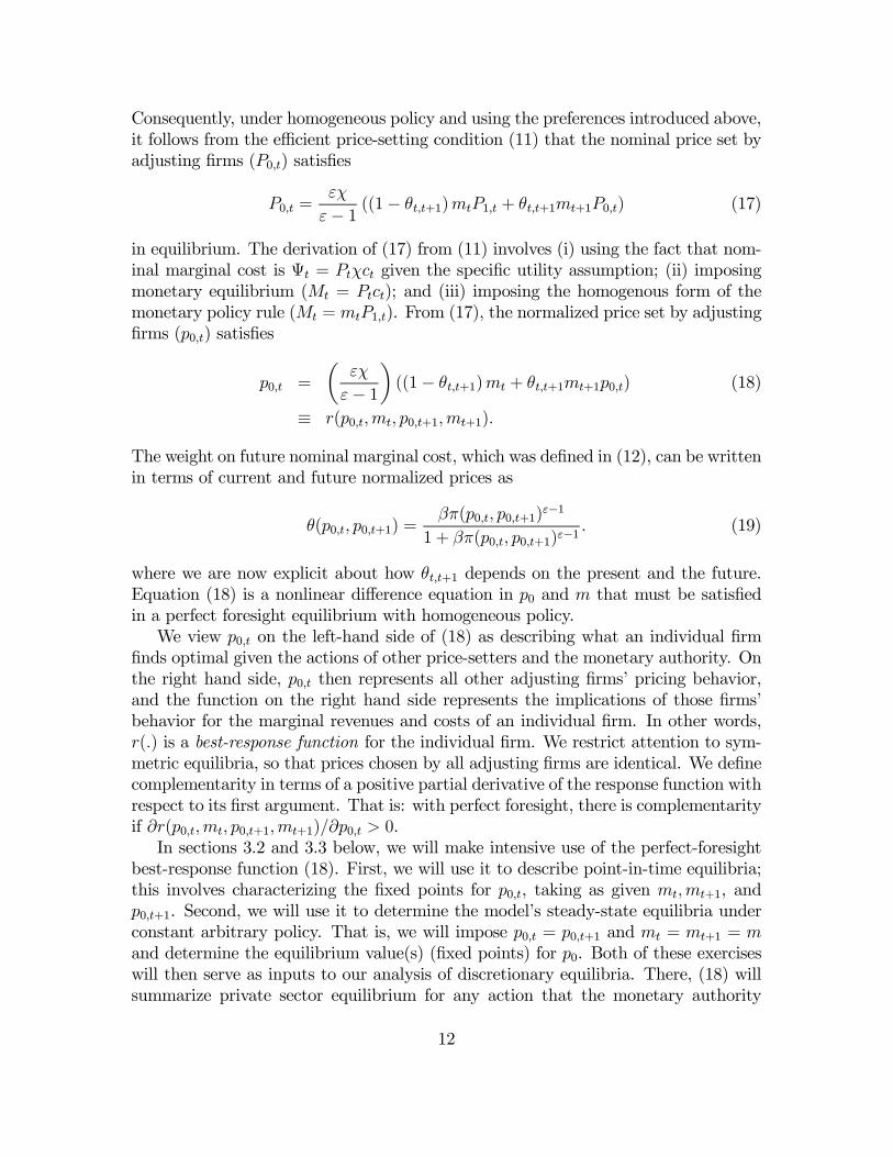
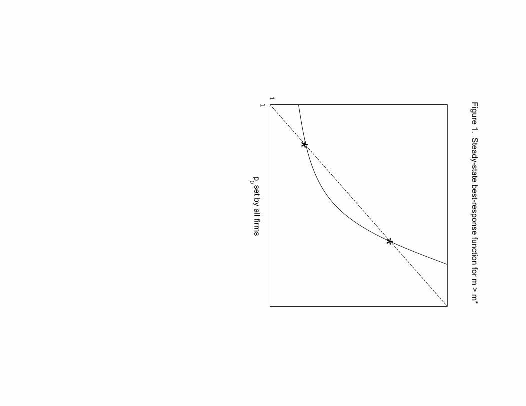
From (20), steady-state equilibria for a givenm are fixed points of r (p0;m) , wherewe write the best-response function as

r (p0,m) =m

m∗· [(1− θ (p0)) + θ (p0) · p0] (22)

for the discussion of proposition 1.

14

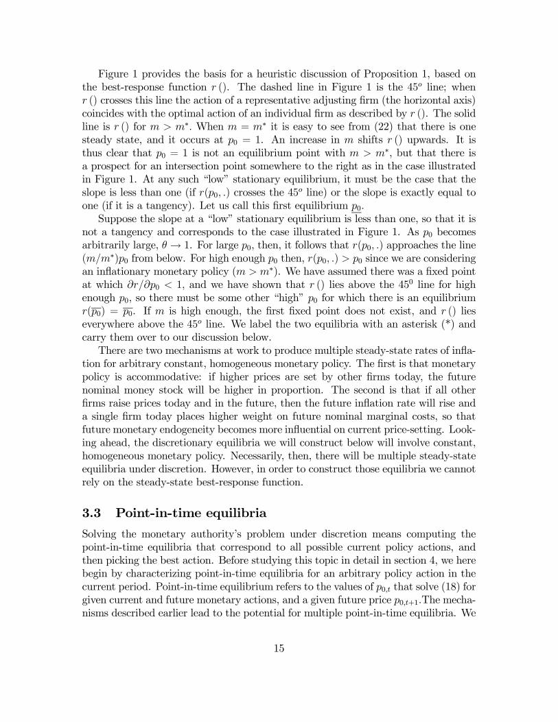
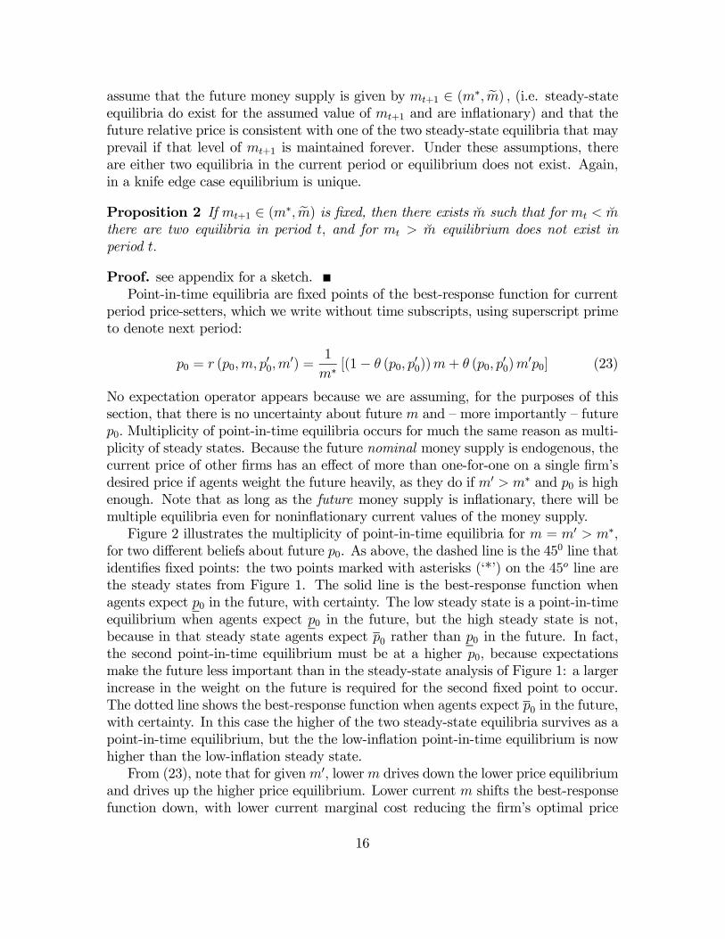
Figure 1 provides the basis for a heuristic discussion of Proposition 1, based onthe best-response function r (). The dashed line in Figure 1 is the 45o line; whenr () crosses this line the action of a representative adjusting firm (the horizontal axis)coincides with the optimal action of an individual firm as described by r (). The solidline is r () for m > m∗. When m = m∗ it is easy to see from (22) that there is onesteady state, and it occurs at p0 = 1. An increase in m shifts r () upwards. It isthus clear that p0 = 1 is not an equilibrium point with m > m∗, but that there isa prospect for an intersection point somewhere to the right as in the case illustratedin Figure 1. At any such “low” stationary equilibrium, it must be the case that theslope is less than one (if r(p0, .) crosses the 45o line) or the slope is exactly equal toone (if it is a tangency). Let us call this first equilibrium p0.Suppose the slope at a “low” stationary equilibrium is less than one, so that it is

not a tangency and corresponds to the case illustrated in Figure 1. As p0 becomesarbitrarily large, θ→ 1. For large p0, then, it follows that r(p0, .) approaches the line(m/m∗)p0 from below. For high enough p0 then, r(p0, .) > p0 since we are consideringan inflationary monetary policy (m > m∗). We have assumed there was a fixed pointat which ∂r/∂p0 < 1, and we have shown that r () lies above the 450 line for highenough p0, so there must be some other “high” p0 for which there is an equilibriumr(p0) = p0. If m is high enough, the first fixed point does not exist, and r () lieseverywhere above the 45o line. We label the two equilibria with an asterisk (*) andcarry them over to our discussion below.There are two mechanisms at work to produce multiple steady-state rates of infla-

tion for arbitrary constant, homogeneous monetary policy. The first is that monetarypolicy is accommodative: if higher prices are set by other firms today, the futurenominal money stock will be higher in proportion. The second is that if all otherfirms raise prices today and in the future, then the future inflation rate will rise anda single firm today places higher weight on future nominal marginal costs, so thatfuture monetary endogeneity becomes more influential on current price-setting. Look-ing ahead, the discretionary equilibria we will construct below will involve constant,homogeneous monetary policy. Necessarily, then, there will be multiple steady-stateequilibria under discretion. However, in order to construct those equilibria we cannotrely on the steady-state best-response function.

3.3 Point-in-time equilibria

Solving the monetary authority’s problem under discretion means computing thepoint-in-time equilibria that correspond to all possible current policy actions, andthen picking the best action. Before studying this topic in detail in section 4, we herebegin by characterizing point-in-time equilibria for an arbitrary policy action in thecurrent period. Point-in-time equilibrium refers to the values of p0,t that solve (18) forgiven current and future monetary actions, and a given future price p0,t+1.The mecha-nisms described earlier lead to the potential for multiple point-in-time equilibria. We

15

assume that the future money supply is given by mt+1 ∈ (m∗, em) , (i.e. steady-stateequilibria do exist for the assumed value of mt+1 and are inflationary) and that thefuture relative price is consistent with one of the two steady-state equilibria that mayprevail if that level of mt+1 is maintained forever. Under these assumptions, thereare either two equilibria in the current period or equilibrium does not exist. Again,in a knife edge case equilibrium is unique.

Proposition 2 If mt+1 ∈ (m∗, em) is fixed, then there exists m̆ such that for mt < m̆there are two equilibria in period t, and for mt > m̆ equilibrium does not exist inperiod t.

Proof. see appendix for a sketch.Point-in-time equilibria are fixed points of the best-response function for current

period price-setters, which we write without time subscripts, using superscript primeto denote next period:

p0 = r (p0,m, p00,m

0) =1

m∗[(1− θ (p0, p

00))m+ θ (p0, p

00)m

0p0] (23)

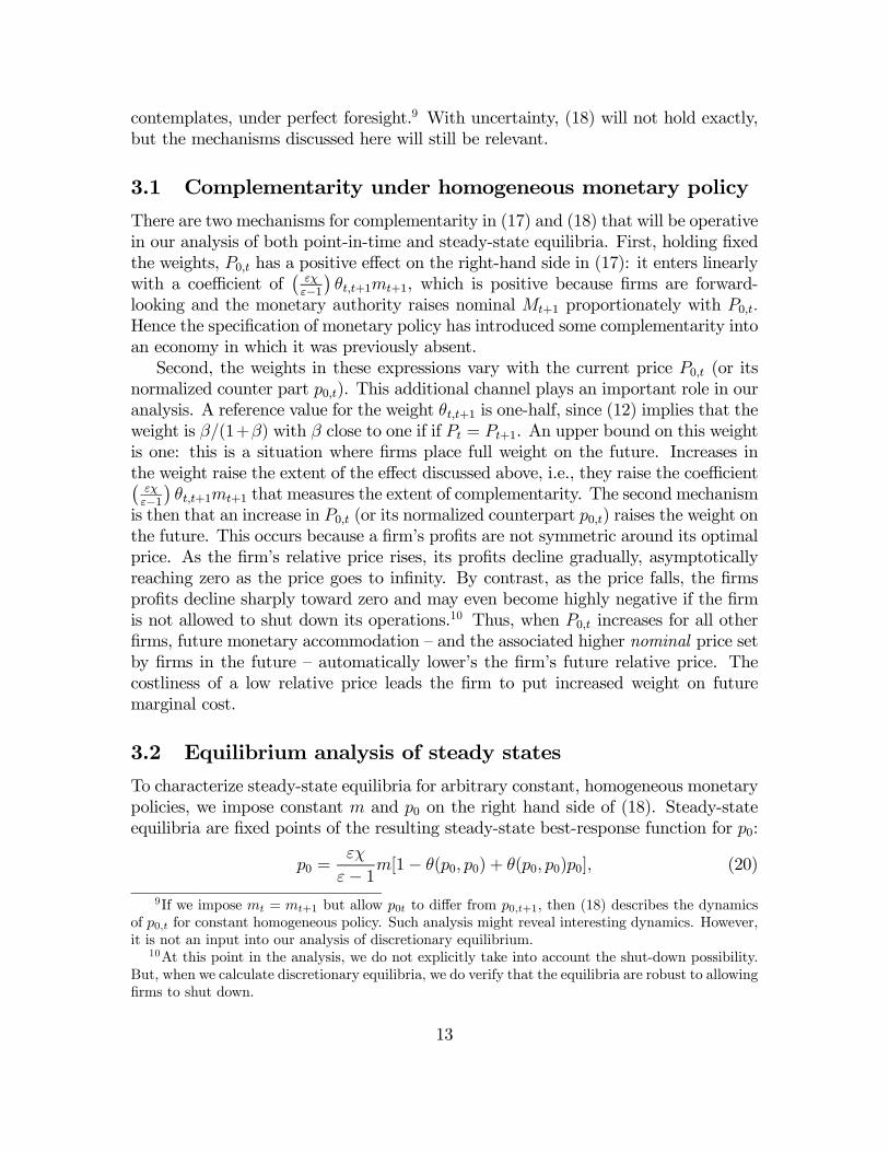
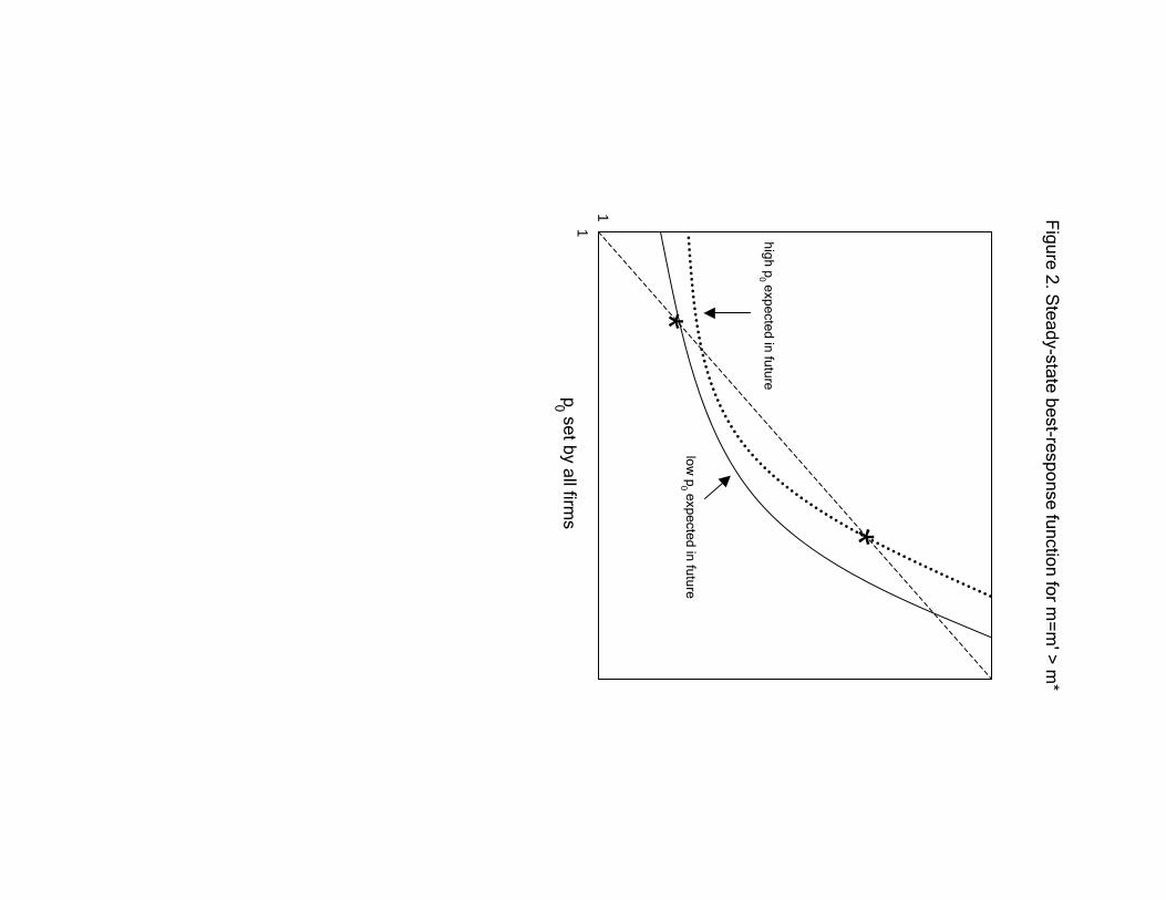
No expectation operator appears because we are assuming, for the purposes of thissection, that there is no uncertainty about future m and — more importantly — futurep0. Multiplicity of point-in-time equilibria occurs for much the same reason as multi-plicity of steady states. Because the future nominal money supply is endogenous, thecurrent price of other firms has an effect of more than one-for-one on a single firm’sdesired price if agents weight the future heavily, as they do if m0 > m∗ and p0 is highenough. Note that as long as the future money supply is inflationary, there will bemultiple equilibria even for noninflationary current values of the money supply.Figure 2 illustrates the multiplicity of point-in-time equilibria for m = m0 > m∗,

for two different beliefs about future p0. As above, the dashed line is the 450 line thatidentifies fixed points: the two points marked with asterisks (‘*’) on the 45o line arethe steady states from Figure 1. The solid line is the best-response function whenagents expect p0 in the future, with certainty. The low steady state is a point-in-timeequilibrium when agents expect p0 in the future, but the high steady state is not,because in that steady state agents expect p0 rather than p0 in the future. In fact,the second point-in-time equilibrium must be at a higher p0, because expectationsmake the future less important than in the steady-state analysis of Figure 1: a largerincrease in the weight on the future is required for the second fixed point to occur.The dotted line shows the best-response function when agents expect p0 in the future,with certainty. In this case the higher of the two steady-state equilibria survives as apoint-in-time equilibrium, but the the low-inflation point-in-time equilibrium is nowhigher than the low-inflation steady state.From (23), note that for givenm0, lowerm drives down the lower price equilibrium

and drives up the higher price equilibrium. Lower current m shifts the best-responsefunction down, with lower current marginal cost reducing the firm’s optimal price

16

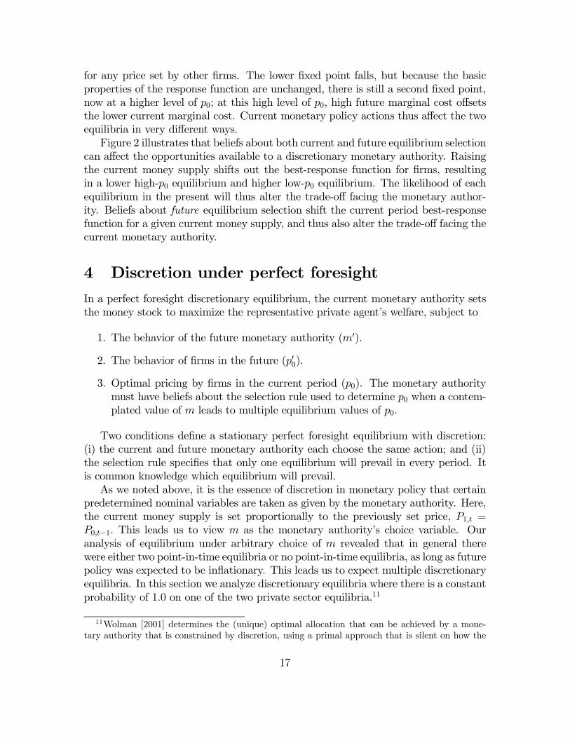
for any price set by other firms. The lower fixed point falls, but because the basicproperties of the response function are unchanged, there is still a second fixed point,now at a higher level of p0; at this high level of p0, high future marginal cost offsetsthe lower current marginal cost. Current monetary policy actions thus affect the twoequilibria in very different ways.Figure 2 illustrates that beliefs about both current and future equilibrium selection

can affect the opportunities available to a discretionary monetary authority. Raisingthe current money supply shifts out the best-response function for firms, resultingin a lower high-p0 equilibrium and higher low-p0 equilibrium. The likelihood of eachequilibrium in the present will thus alter the trade-off facing the monetary author-ity. Beliefs about future equilibrium selection shift the current period best-responsefunction for a given current money supply, and thus also alter the trade-off facing thecurrent monetary authority.

4 Discretion under perfect foresightIn a perfect foresight discretionary equilibrium, the current monetary authority setsthe money stock to maximize the representative private agent’s welfare, subject to

1. The behavior of the future monetary authority (m0).

2. The behavior of firms in the future (p00).

3. Optimal pricing by firms in the current period (p0). The monetary authoritymust have beliefs about the selection rule used to determine p0 when a contem-plated value of m leads to multiple equilibrium values of p0.

Two conditions define a stationary perfect foresight equilibrium with discretion:(i) the current and future monetary authority each choose the same action; and (ii)the selection rule specifies that only one equilibrium will prevail in every period. Itis common knowledge which equilibrium will prevail.As we noted above, it is the essence of discretion in monetary policy that certain

predetermined nominal variables are taken as given by the monetary authority. Here,the current money supply is set proportionally to the previously set price, P1,t =P0,t−1. This leads us to view m as the monetary authority’s choice variable. Ouranalysis of equilibrium under arbitrary choice of m revealed that in general therewere either two point-in-time equilibria or no point-in-time equilibria, as long as futurepolicy was expected to be inflationary. This leads us to expect multiple discretionaryequilibria. In this section we analyze discretionary equilibria where there is a constantprobability of 1.0 on one of the two private sector equilibria.11

11Wolman [2001] determines the (unique) optimal allocation that can be achieved by a mone-tary authority that is constrained by discretion, using a primal approach that is silent on how the

17

4.1 Constructing Discretionary Equilibria

We look for a stationary, discretionary equilibrium, which is a value of m that max-imizes u(c, l) subject to the constraints above when m0 = m.12 We have used twocomputational approaches to find this fixed point. A comparison of the two ap-proaches is revealing about the nature of the multiple equilibria we encounter.The first computational method involves iterating on steady states. We assume

that all future monetary authorities follow some fixed rule m0. Next, we determinethe steady state that prevails including the value of p00. Then, we confront the cur-rent monetary policy authority with these beliefs and ask her to optimize, given theconstraints including the selection rule. If she chooses an m such that |m − m0| issufficiently small, then we have an approximate fixed point. If not, then we adjustthe future monetary policy rule in the direction of her choice and go through theprocess again until we have achieved an approximate fixed point. This approach con-ceptually matches our discussion throughout the text, but leaves open an importanteconomic question: are the equilibria that we construct critically dependent on theinfinite horizon nature of the problem?The second computational method involves backward induction on finite horizon

economies. We begin with a last period, in which firms are not forward-looking intheir price setting and deduce that there is a single equilibrium, including an optimalaction for the monetary authority mT > m

∗ and a unique equilibrium relative pricep0,T . Then, we step back one period, taking as given the future monetary action andthe future relative price. We find that there are two private sector equilibria. In fact,this is inevitable, because the first step backwards creates a version of our point-in-time analysis above. Consequently, this approach establishes that the phenomenaare associated with forward-looking pricing and homogenous monetary policy, ratherthan with an infinite horizon. To construct stationary nonstochastic equilibria usingthis approach, we can iterate backwards from the last period, computing the optimalpolicy, {mT ,mT−1, ....} and stop the process when |mt+1−mt| is small, takingmt = mas an approximate fixed point.The numerical examples that we study next have the following common elements.

The demand elasticity (ε) is 10, implying a gross markup of 1.11 in a zero inflationsteady state. The preference parameter (χ) is 0.9, and for convenience we set the timeendowment to 5. Taken together with the markup, this implies that agents will workone fifth of their time (n = 1) in a zero inflation steady state. With zero inflation,c = n = 1 since there are no relative price distortions, and thus m∗ = 1. Further,leisure (l) is then 5 − c. Accordingly, in a zero inflation stationary state, utility is

monetary authority brings about this allocation using monetary instruments. This allocation is theone associated with the low-p0 equilibrium described here. Our work thus shows that a monetaryauthority which seeks to implement the optimal real allocation using a money stock rule leaves itselfvulnerable to multiple equilibria.

12Dotsey and Hornstein [2003] use linear-quadratic methods to study the monetary policy problemunder discretion. We believe that these essentially rule out the phenomena encountered in this paper.

18

just ln(1)+0.9 · (5−1). A first-best outcome would dictate that u(c, l) be maximizedsubject to c = (1−l). For the specified preferences, this leads to a first order condition1n= χ or an efficient level of work (n) of 1.11. So, the increase in work from cutting

the gross markup to one is 11.1%.

4.2 Optimistic Equilibrium

If the discretionary monetary authority knows that the low equilibrium will prevail,then its problem is to maximize

u(c, l) + v(p00;m0)

where v(p00;m0) denotes the future utility that corresponds to a steady state withm0 and selection of the low-p0 equilibrium with probability 1.0. The maximization issubject to

c = c(m, p0)

l = l(m, p0)

p0 = r(p0, p00,m,m0),

where r () denotes the response function on the right hand side of (23), and thepresence of p0 instead of p0 is meant to imply that we place probability one on thelow-p0 fixed point of the response function. The monetary authority understandsthat future utility and current price determination is influenced by the actions of thefuture monetary authority, but has no way of influencing its behavior or the futureprice that will prevail. So, the monetary authority maximizes current period utility.

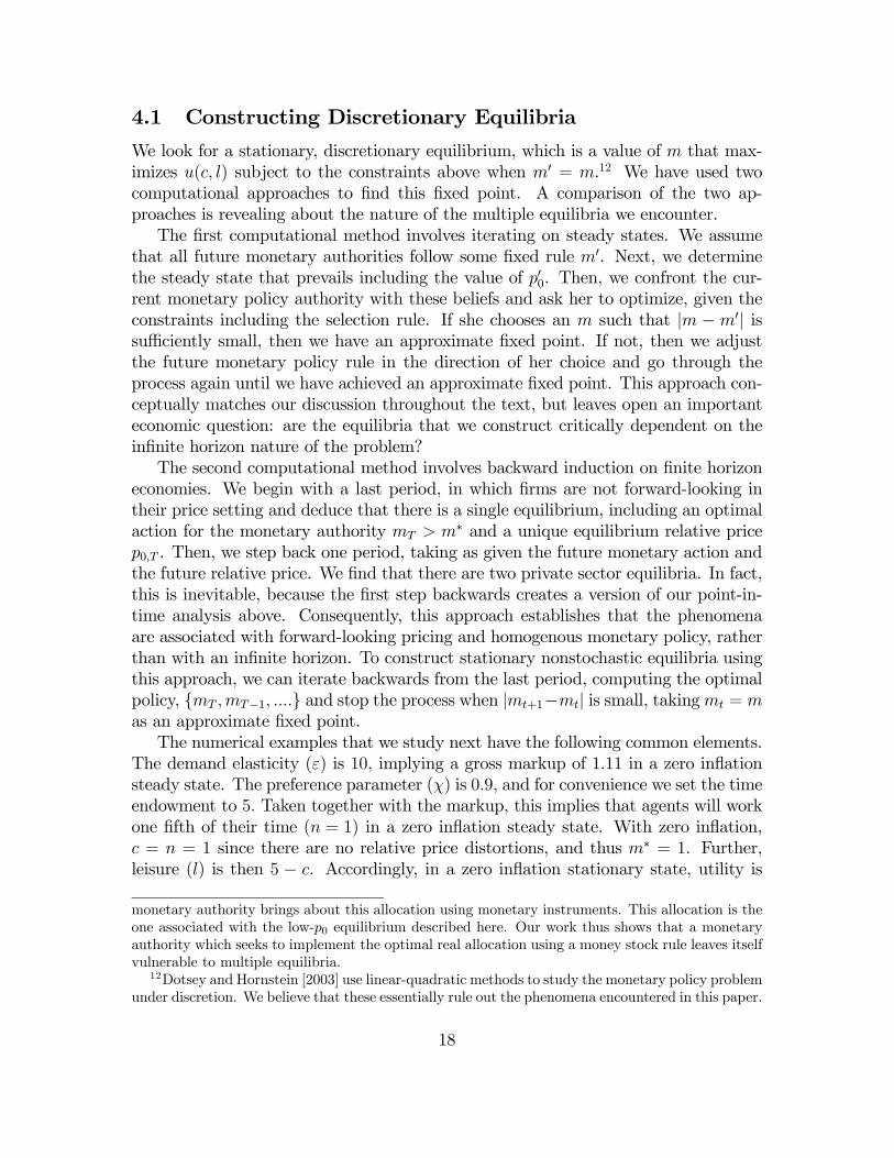
4.2.1 Exploiting initial conditions

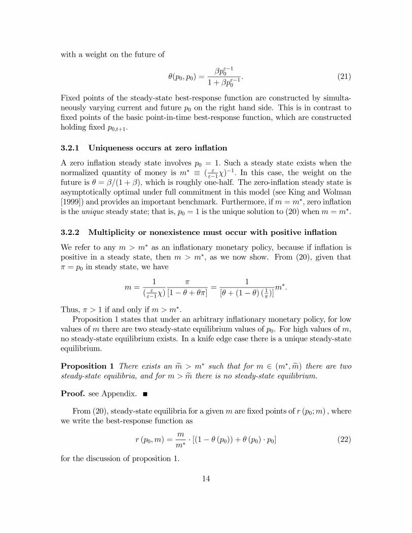
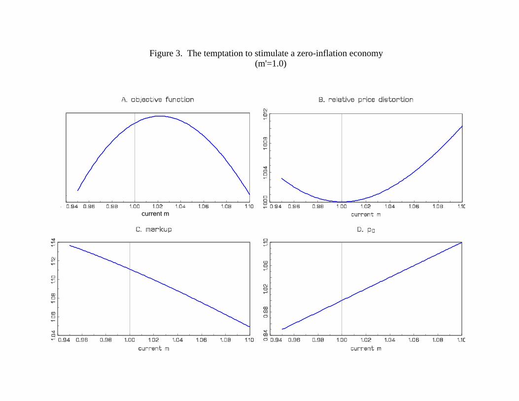
Figure 3 provides some insight into the nature of the monetary authority’s choicewhen it knows that the p0 equilibrium will prevail for all time. For this figure, weassume that future monetary policy is noninflationary (m0 = m∗, p00 = 1). The cur-rent monetary authority optimally adopts an inflationary monetary policy (choosingm > m∗ = 1) because it can reduce the markup and stimulate consumption towardthe first-best level. It does not completely drive the gross markup to one becausean increase in m produces relative price distortions. While the relative price distor-tions are negligible near the noninflationary steady state, they increase convexly asmonetary policy stimulates the economy. Figure 3 illustrates the sense in which NewKeynesian models capture the incentive for stimulating the economy at zero inflation,as described in Kydland and Prescott [1977] and Barro and Gordon [1983].

4.2.2 An inflation bias equilibrium

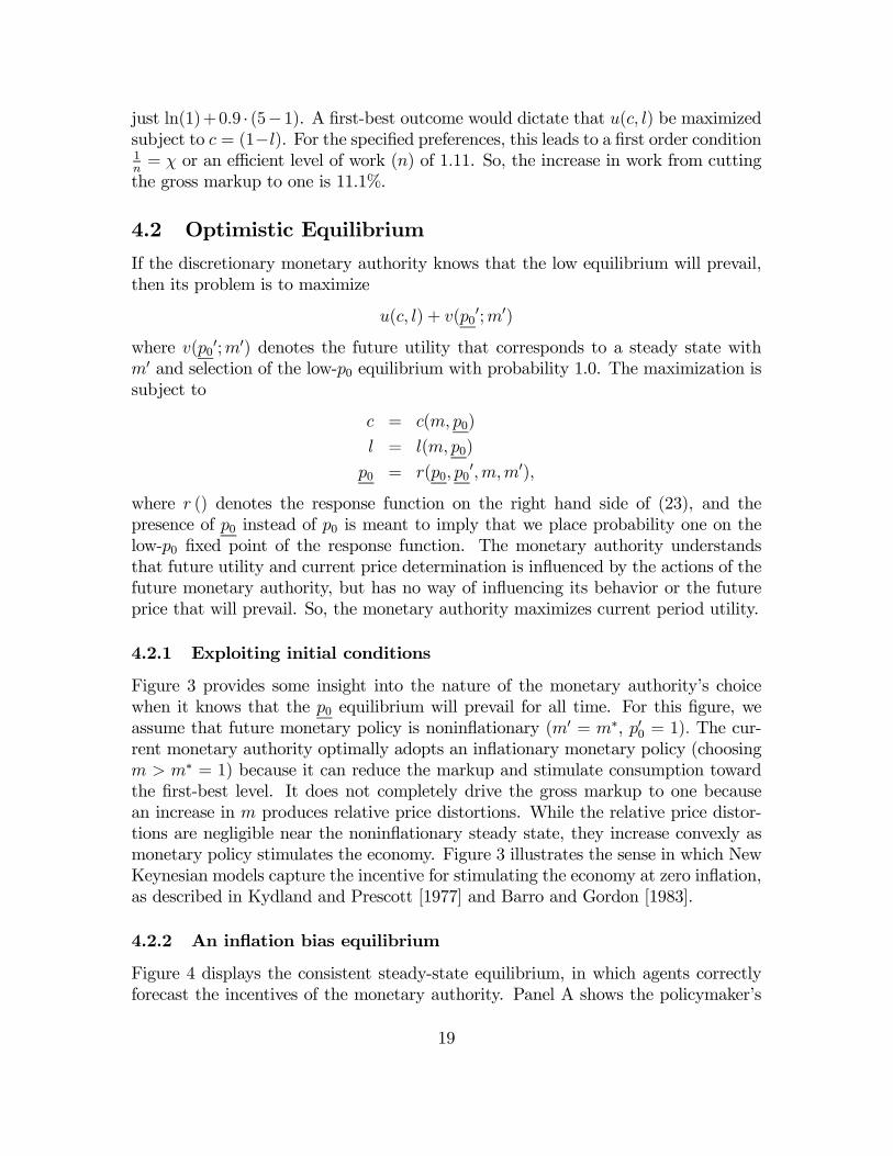
Figure 4 displays the consistent steady-state equilibrium, in which agents correctlyforecast the incentives of the monetary authority. Panel A shows the policymaker’s

19

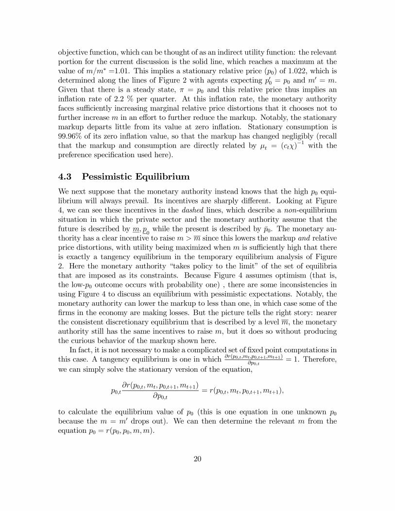
objective function, which can be thought of as an indirect utility function: the relevantportion for the current discussion is the solid line, which reaches a maximum at thevalue of m/m∗ =1.01. This implies a stationary relative price (p0) of 1.022, which isdetermined along the lines of Figure 2 with agents expecting p00 = p0 and m

0 = m.Given that there is a steady state, π = p0 and this relative price thus implies aninflation rate of 2.2 % per quarter. At this inflation rate, the monetary authorityfaces sufficiently increasing marginal relative price distortions that it chooses not tofurther increase m in an effort to further reduce the markup. Notably, the stationarymarkup departs little from its value at zero inflation. Stationary consumption is99.96% of its zero inflation value, so that the markup has changed negligibly (recallthat the markup and consumption are directly related by µt = (ctχ)

−1 with thepreference specification used here).

4.3 Pessimistic Equilibrium

We next suppose that the monetary authority instead knows that the high p0 equi-librium will always prevail. Its incentives are sharply different. Looking at Figure4, we can see these incentives in the dashed lines, which describe a non-equilibriumsituation in which the private sector and the monetary authority assume that thefuture is described by m, p

0while the present is described by p̄0. The monetary au-

thority has a clear incentive to raise m > m since this lowers the markup and relativeprice distortions, with utility being maximized when m is sufficiently high that thereis exactly a tangency equilibrium in the temporary equilibrium analysis of Figure2. Here the monetary authority “takes policy to the limit” of the set of equilibriathat are imposed as its constraints. Because Figure 4 assumes optimism (that is,the low-p0 outcome occurs with probability one) , there are some inconsistencies inusing Figure 4 to discuss an equilibrium with pessimistic expectations. Notably, themonetary authority can lower the markup to less than one, in which case some of thefirms in the economy are making losses. But the picture tells the right story: nearerthe consistent discretionary equilibrium that is described by a level m, the monetaryauthority still has the same incentives to raise m, but it does so without producingthe curious behavior of the markup shown here.In fact, it is not necessary to make a complicated set of fixed point computations in

this case. A tangency equilibrium is one in which ∂r(p0,t,mt,p0,t+1,mt+1)

∂p0,t= 1. Therefore,

we can simply solve the stationary version of the equation,

p0,t∂r(p0,t,mt, p0,t+1,mt+1)

∂p0,t= r(p0,t,mt, p0,t+1,mt+1),

to calculate the equilibrium value of p0 (this is one equation in one unknown p0because the m = m0 drops out). We can then determine the relevant m from theequation p0 = r(p0, p0,m,m).

20

In our numerical example, there is a consistent equilibrium with p0 = 1.17, so thatthere is a 17% quarterly inflation rate in the pessimistic equilibrium with optimaldiscretionary policy. The associated value of m/m∗ is 1.0295. This value is largerthan the one used to construct Figure 3, as it should be: a higher level of m isnecessary to produce a tangency equilibrium in the pessimistic case.There are thus two steady-state equilibria with discretionary optimal monetary

policy in our quantitative example, one with low inflation and one with high inflation.The levels of the inflation rates are quite different: about 2 percent (per quarter) inone case and about 17 percent in the other.

5 Stochastic equilibria

The generic existence of two point-in-time equilibria and two steady-state equilibriafor arbitrary homogeneous policy suggests that it may be possible to construct discre-tionary equilibria that involve stochastic fluctuations. We now provide an example ofsuch an equilibrium. We assume that there is an i.i.d. sunspot realized each periodwhich selects between the two private sector equilibria: in each period, the low-p0outcome occurs with probability 0.6, the high-p0 outcome occurs with probability of0.4, and this is common knowledge.13

In order for its maximization problem to be well-defined, the monetary author-ity must have beliefs about the current and future distribution over private-sectorequilibria. Above, these beliefs were degenerate. Now that they are nondegenerate,the problem is slightly more complicated. Letting α be the probability of the low-p0outcome, the monetary authority maximizes

{αu(c(m, p0), l(m, p0)) + (1− α)u(c(m, p0), l(m, p0))}+ βv0

where v0 denotes the future expected utility, which again cannot be influenced by thecurrent monetary authority. It is important to stress that the low and high p0 valuesare influenced by the sunspot probabilities, since they satisfy the equations

p0 =1

m∗

·µ1

1 + βEπ (p0, p00)ε−1

¶m+

µβp0

1 + βEπ (p0, p00)ε−1

¶Enπ (p0, p

00)

ε−1m0o¸,

(24)where expectations are taken over the distribution of the sunspot variable. For ex-ample,

Eπ (p0, p00)

ε−1= απ

³p0, p0

´ε−1+ (1− α)π (p0, p0)

ε−1 .

13Our model does not pin down the distribution of the sunspot variable. However, some restric-tions on that distribution are imposed by the requirement that every firm’s profits be nonnegative ineach period. For example, if α is 0.75 rather than 0.6, this condition is violated in the p0 state, andno discretionary equilibrium exists. As in Ennis and Keister (forthcoming), it would be interestingto study whether adaptive learning schemes would further restrict the distribution of the sunspotvariable.

21

Because the sunspot is i.i.d., this expression holds for both the low and high currentvalue of p0. Note that uncertainty prevents us fromwriting (24) as the simple weightedaverage that we used with perfect foresight.

5.1 Constructing Discretionary Equilibria

We can again apply the two computational approaches described in the previoussection to construct Nash equilibria. In implementing these, we assume that themonetary authority and the private sector share the same probability beliefs.

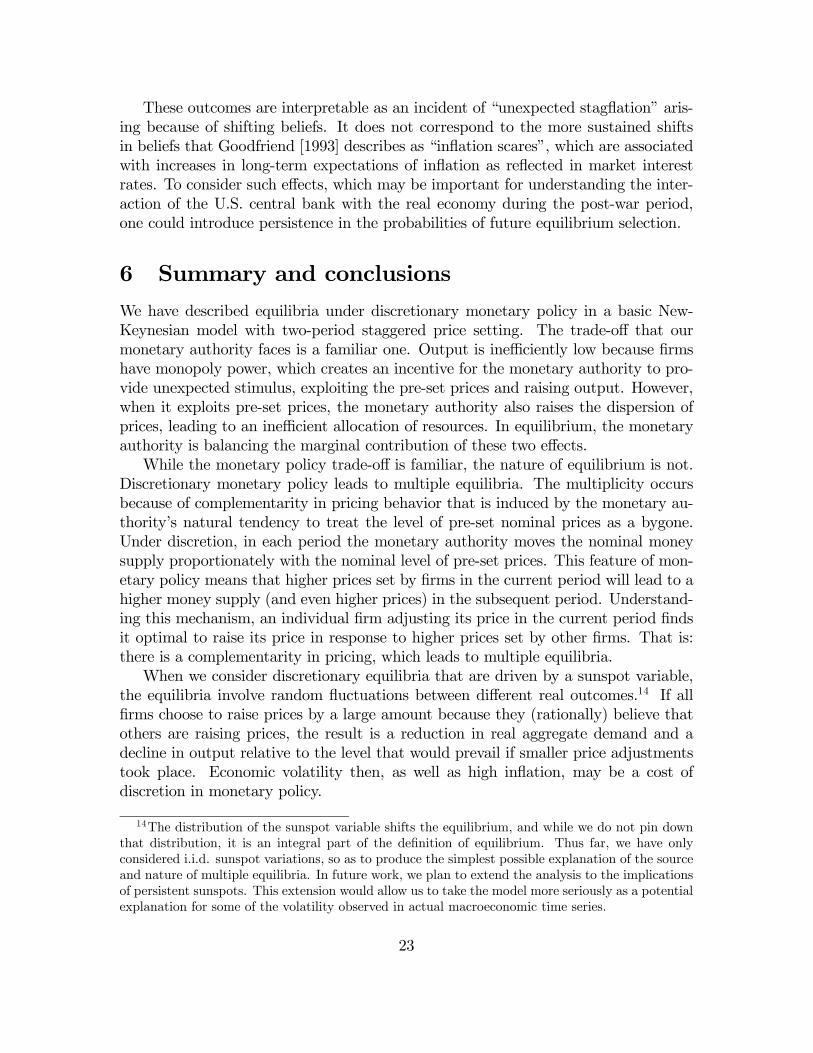
5.2 Optimal discretionary policy

The relevant trade-offs for the discretionary monetary authority are illustrated inFigure 5. In panel A, there is a light solid line between the objective function forthe low-p0 private-sector equilibrium (the dark solid line) and the objective functionfor the high-p0 private sector equilibrium (the dashed line): this is the monetaryauthority’s expected utility objective, which is a weighted average of the two otherobjectives. The monetary authority chooses an optimal action that is about 1.0202,which is more stimulative than the earlier equilibrium action (1.01, shown in Figure4) that was appropriate under extreme optimism (α = 1). But it is smaller than theequilibrium action appropriate under extreme pessimism (α = 0).Figure 5 also highlights that the specific values taken on by p0 in the optimistic

and pessimistic equilibrium are endogenously determined in our setup, by currentmonetary policy and the sunspot probabilities. By contrast, in the essentially staticmodels of Albanesi, Chari and Christiano [2002], the values of endogenous variablesare not affected by the probability structure of extrinsic uncertainty.

5.3 Effects of sunspots

Consider now the effects of a sunspot on equilibrium quantities. We take as the refer-ence point the levels in the low-p0 private-sector equilibrium, which involve a markupof about 1.11 (close to the zero inflation markup) and a normalized price that is closeto one. If the economy suddenly shifts to the high-p0 private sector equilibrium as aresult of the sunspot, then firms become much more aggressive in their adjustments.With the nominal money stock fixed (Mt = mP1,t−1), there is a decline in real ag-gregate demand since the price level rises. Consumption and work effort accordinglyfall. Alternatively, the average markup rises dramatically, increasing distortions inthe economy, to bring about this set of results. Quantitatively, in Figure 5, the risein the markup is from about 1.12 to about 1.17, so that there is roughly a 4.5%increase in the markup. Given that markups and consumption are (inversely) relatedproportionately, there is a 4.5% decline in consumption and work effort.

22

These outcomes are interpretable as an incident of “unexpected stagflation” aris-ing because of shifting beliefs. It does not correspond to the more sustained shiftsin beliefs that Goodfriend [1993] describes as “inflation scares”, which are associatedwith increases in long-term expectations of inflation as reflected in market interestrates. To consider such effects, which may be important for understanding the inter-action of the U.S. central bank with the real economy during the post-war period,one could introduce persistence in the probabilities of future equilibrium selection.

6 Summary and conclusionsWe have described equilibria under discretionary monetary policy in a basic New-Keynesian model with two-period staggered price setting. The trade-off that ourmonetary authority faces is a familiar one. Output is inefficiently low because firmshave monopoly power, which creates an incentive for the monetary authority to pro-vide unexpected stimulus, exploiting the pre-set prices and raising output. However,when it exploits pre-set prices, the monetary authority also raises the dispersion ofprices, leading to an inefficient allocation of resources. In equilibrium, the monetaryauthority is balancing the marginal contribution of these two effects.While the monetary policy trade-off is familiar, the nature of equilibrium is not.

Discretionary monetary policy leads to multiple equilibria. The multiplicity occursbecause of complementarity in pricing behavior that is induced by the monetary au-thority’s natural tendency to treat the level of pre-set nominal prices as a bygone.Under discretion, in each period the monetary authority moves the nominal moneysupply proportionately with the nominal level of pre-set prices. This feature of mon-etary policy means that higher prices set by firms in the current period will lead to ahigher money supply (and even higher prices) in the subsequent period. Understand-ing this mechanism, an individual firm adjusting its price in the current period findsit optimal to raise its price in response to higher prices set by other firms. That is:there is a complementarity in pricing, which leads to multiple equilibria.When we consider discretionary equilibria that are driven by a sunspot variable,

the equilibria involve random fluctuations between different real outcomes.14 If allfirms choose to raise prices by a large amount because they (rationally) believe thatothers are raising prices, the result is a reduction in real aggregate demand and adecline in output relative to the level that would prevail if smaller price adjustmentstook place. Economic volatility then, as well as high inflation, may be a cost ofdiscretion in monetary policy.

14The distribution of the sunspot variable shifts the equilibrium, and while we do not pin downthat distribution, it is an integral part of the definition of equilibrium. Thus far, we have onlyconsidered i.i.d. sunspot variations, so as to produce the simplest possible explanation of the sourceand nature of multiple equilibria. In future work, we plan to extend the analysis to the implicationsof persistent sunspots. This extension would allow us to take the model more seriously as a potentialexplanation for some of the volatility observed in actual macroeconomic time series.

23

References[1] Albanesi, Stefania, V.V. Chari and Lawrence Christiano (2002), “Expectations

Traps and Monetary Policy,” NBER Working Paper 8912.

[2] Barro, Robert and David B. Gordon (1983), “A Positive Theory of MonetaryPolicy in a Natural Rate Model,” Journal of Political Economy 91, 589-610.

[3] Blanchard, Olivier J. and Nobuhiro Kiyotaki (1987), “Monopolistic Competitionand the Effects of Aggregate Demand,” American Economic Review 77, 647-666.

[4] Clarida, Richard, Jordi Gali and Mark Gertler (1999), “The Science of MonetaryPolicy: A NewKeynesian Perspective,” Journal of Economic Literature 37, 1661-1707.

[5] Cooper, Russell W. and A. Andrew John (1988), “Coordinating CoordinationFailures in Keynesian Models,” Quarterly Journal of Economics 103, 441-463.

[6] Dotsey, Michael and Andreas Hornstein (2003), “Should a monetary policymakerlook at money?” Journal of Monetary Economics 50, 547-79.

[7] Ennis, Huberto M. and Todd Keister (forthcoming), “Government Policy andthe Probability of Coordination Failures,” European Economic Review.

[8] Glomm, Gerhard and B. Ravikumar (1995), “Endogenous Public Policy andMultiple Equilibria.” European Journal of Political Economy 11, 653-662.

[9] Goodfriend, Marvin (1993), “Interest Rate Policy and the Inflation Scare Prob-lem: 1979-92,” Federal Reserve Bank of Richmond Economic Quarterly (Win-ter), pp. 1-24.

[10] Ireland, Peter (1997), “Sustainable Monetary Policies.” Journal of EconomicDynamics and Control 22 (November): 87—108.

[11] Kimball, Miles S. (1995). “The Quantitative Analytics of the Basic Neomone-tarist Model”, Journal of Money, Credit, and Banking, 27, 1241-1277.

[12] King, Robert G. and Alexander L. Wolman (1999), “What Should the MonetaryAuthority Do When Prices Are Sticky?” inMonetary Policy Rules, John Taylor,ed. University of Chicago Press, 349-398

[13] Kydland, Finn E. and Edward C. Prescott (1977), “Rules Rather than Discre-tion: The Inconsistency of Optimal Plans,” Journal of Political Economy 85,473-492.

[14] Rotemberg, Julio J. (1987), “The New Keynesian Microfoundations,” NBERMacroeconomics Annual, MIT Press: Cambridge, MA.

24

[15] Wolman, Alexander L. (2001), “A Primer on Optimal Monetary Policy in StickyPrice Models,” Federal Reserve Bank of Richmond Economic Quarterly 87, 27-52.

[16] Woodford, Michael, (2002) Interest and Prices, manuscript, Chapter 3.

25

A Appendix

A.1 Proofs

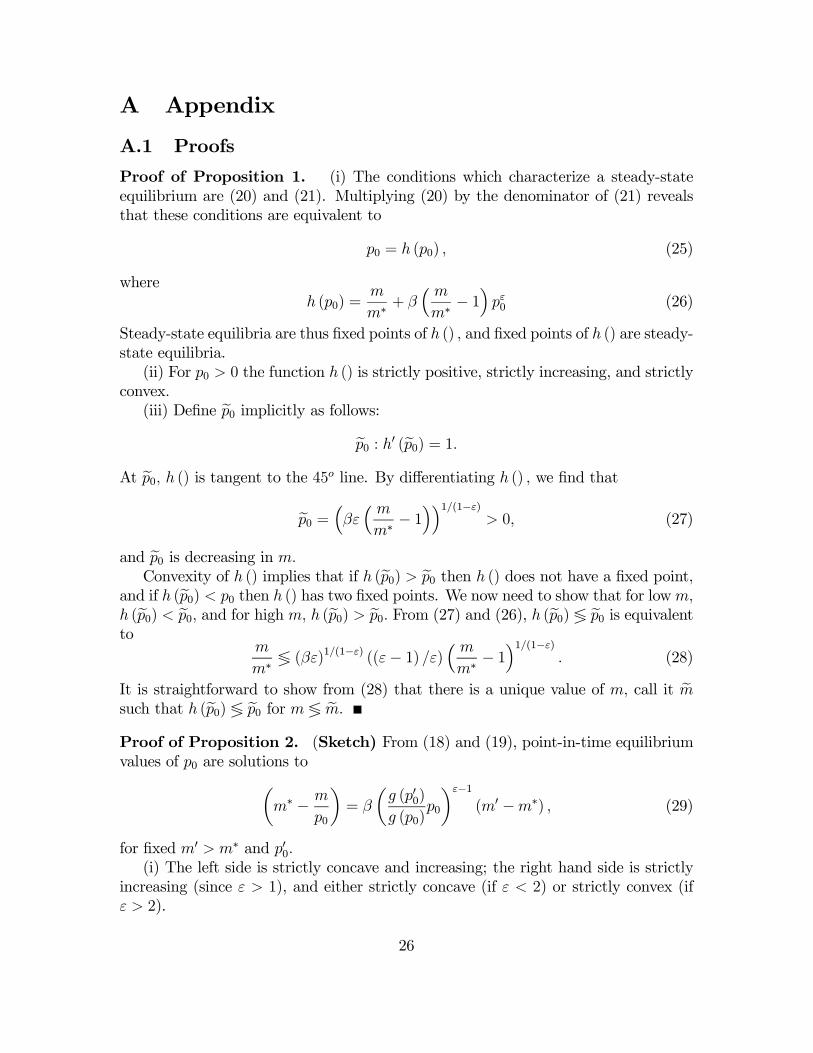
Proof of Proposition 1. (i) The conditions which characterize a steady-stateequilibrium are (20) and (21). Multiplying (20) by the denominator of (21) revealsthat these conditions are equivalent to

p0 = h (p0) , (25)

whereh (p0) =

m

m∗+ β

³ mm∗− 1´pε0 (26)

Steady-state equilibria are thus fixed points of h () , and fixed points of h () are steady-state equilibria.(ii) For p0 > 0 the function h () is strictly positive, strictly increasing, and strictly

convex.(iii) Define ep0 implicitly as follows:

ep0 : h0 (ep0) = 1.At ep0, h () is tangent to the 45o line. By differentiating h () , we find that

ep0 = ³βε³ mm∗− 1´´1/(1−ε)

> 0, (27)

and ep0 is decreasing in m.Convexity of h () implies that if h (ep0) > ep0 then h () does not have a fixed point,

and if h (ep0) < p0 then h () has two fixed points. We now need to show that for lowm,h (ep0) < ep0, and for high m, h (ep0) > ep0. From (27) and (26), h (ep0) ≶ ep0 is equivalentto

m

m∗≶ (βε)1/(1−ε) ((ε− 1) /ε)

³ mm∗− 1´1/(1−ε)

. (28)

It is straightforward to show from (28) that there is a unique value of m, call it emsuch that h (ep0) ≶ ep0 for m ≶ em.Proof of Proposition 2. (Sketch) From (18) and (19), point-in-time equilibriumvalues of p0 are solutions toµ

m∗ − mp0

¶= β

µg (p00)g (p0)

p0

¶ε−1(m0 −m∗) , (29)

for fixed m0 > m∗ and p00.(i) The left side is strictly concave and increasing; the right hand side is strictly

increasing (since ε > 1), and either strictly concave (if ε < 2) or strictly convex (ifε > 2).

26

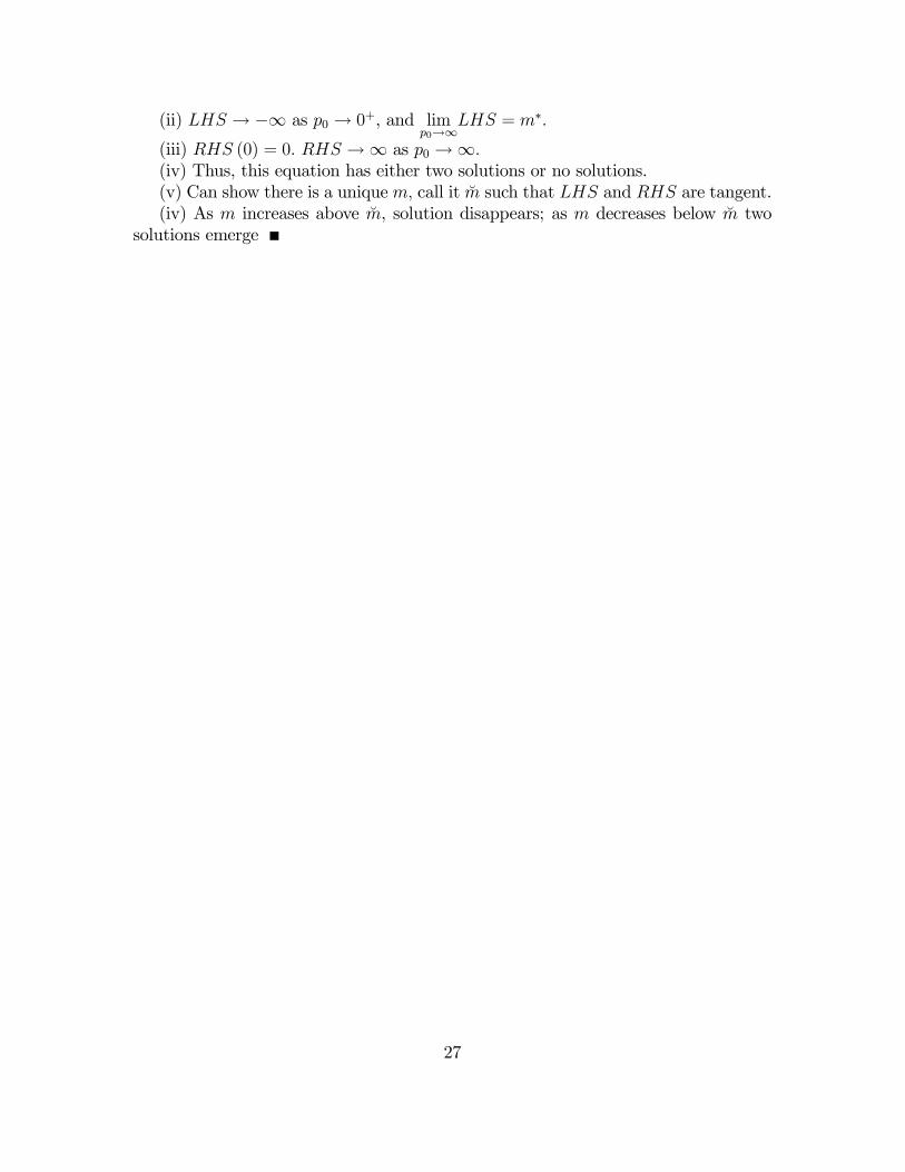
(ii) LHS →−∞ as p0 → 0+, and limp0→∞

LHS = m∗.

(iii) RHS (0) = 0. RHS →∞ as p0 →∞.(iv) Thus, this equation has either two solutions or no solutions.(v) Can show there is a unique m, call it m̆ such that LHS and RHS are tangent.(iv) As m increases above m̆, solution disappears; as m decreases below m̆ two

solutions emerge

27

11

*

*

Figure

1. Steady-state best-response function for m

> m

*

p set by all firms

0

11

*

*

p set by all firms

0

low p expected in future

high p expected in future0

0

Figure 2. S

teady-state best-response function for m=

m' >

m*

current m

Figure 3. The temptation to stimulate a zero-inflation economy (m'=1.0)

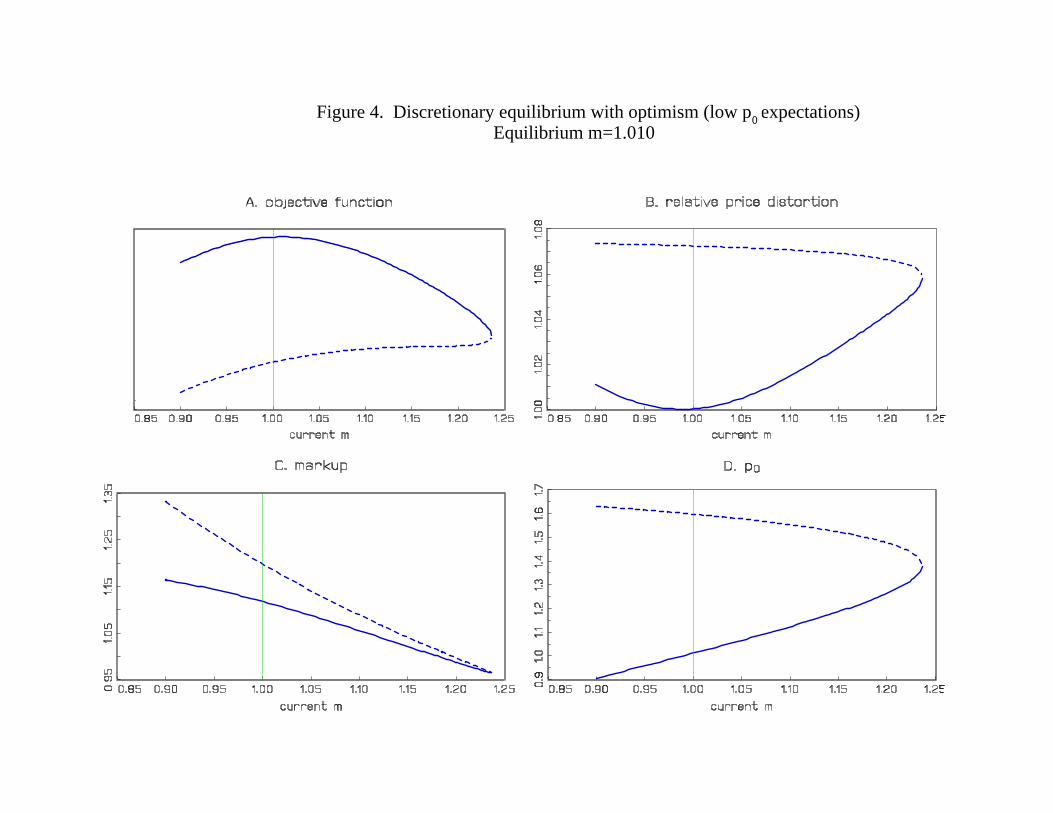
Figure 4. Discretionary equilibrium with optimism (low p expectations) Equilibrium m=1.010

0

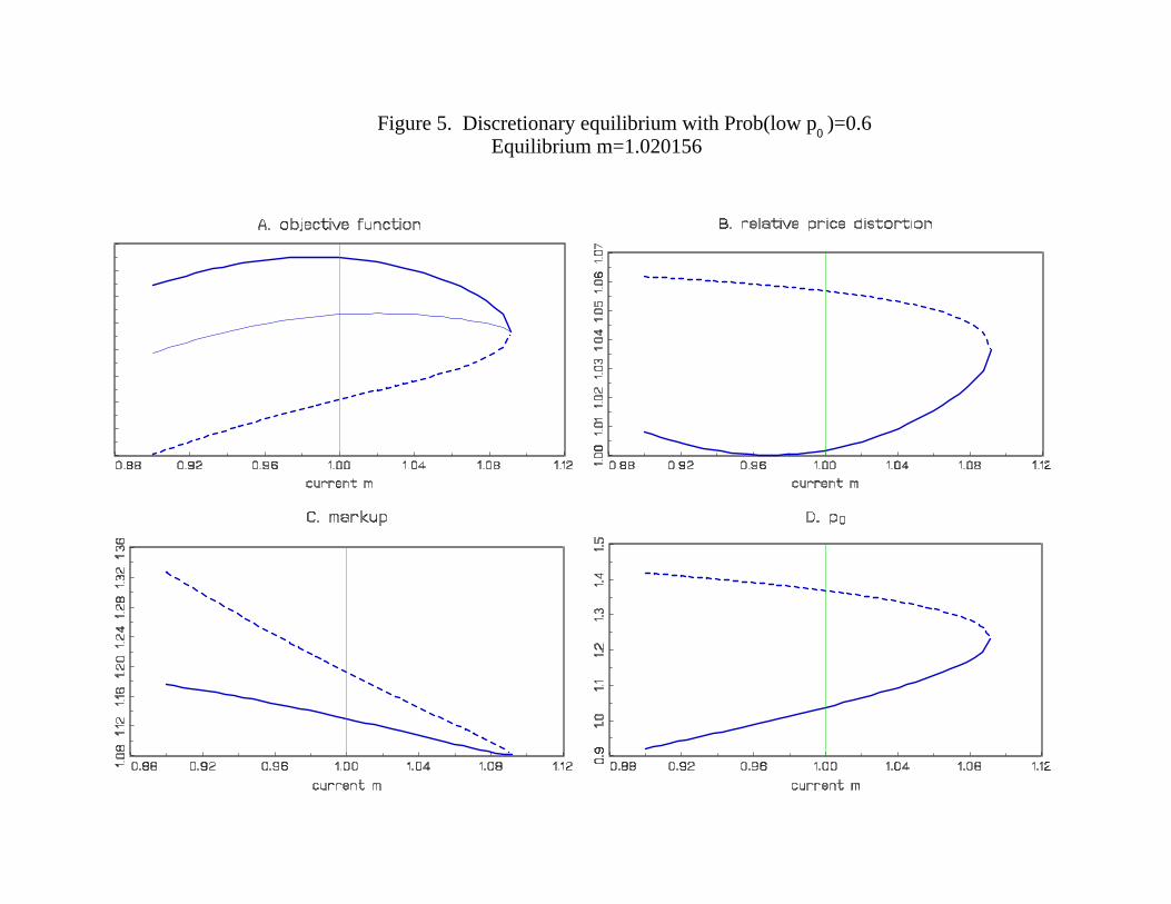
Figure 5. Discretionary equilibrium with Prob(low p )=0.6 Equilibrium m=1.020156

0