assessment of the technical issues relating to significant
TRANSCRIPT

Assessment of the Technical Issues relating to
Significant Amounts of EHV Underground Cable
in the All-island Electricity Transmission System
Public Report
November 2009
Tokyo Electric Power Company

Contract CA209:
Assessment of the Technical Issues relating to
Significant Amounts of EHV Underground Cable
in the All-island Electricity Transmission System
Public Report
November 2009
Tokyo Electric Power Company
LEGAL NOTICE:This report has been created solely for public disclosure purposes and does not include the original report’s contents in its entirety . TEPCO is not liable for any damage that ensues due to unauthorized utilization of knowledge acquired from this report that exceeds designated project scope boundaries.THE TOKYO ELECTRIC POWER COMPANY, INC.

Executive Summary

Executive Summary
©2009 The Tokyo Electric Power Company, INC. All Rights Reserved.
Executive Summary
TEPCO has carried out the following studies in order to evaluate the effect of cable
installations on the NIE/EirGrid network:
Part 1: Evaluation of the potential impact on the all-island transmission system of significant
lengths of EHV underground cable, either individually or in aggregate
Part 2: Feasibility study on the 400 kV Woodland – Kingscourt – Turleenan line as AC EHV
underground cables for the entire length
Part 3: Feasibility study of the 400 kV Woodland – Kingscourt – Turleenan line as mixed OHL /
underground cable
For Part 1, the 400 kV Kilkenny – Cahir – Aghada line was selected as the focus of the study
except for the series resonance overvoltage analysis. The series resonance overvoltage analysis in
Part 1 focused on the 400 kV Woodland – Kingscourt – Turleenan line as in Part 2 and 3. For
each part of the study, the reactive power compensation analysis, the temporary overvoltage
analysis, and the slow-front overvoltage analysis were conducted. Further, the lightning
overvoltage analysis was conducted additionally for Part 3.
[Part 1]
First, the results of the reactive power compensation analysis led to the necessity of having to
achieve compensation rates close to 100 % in order to ensure the safe operation of the network.
The following compensation patterns all yielded satisfactory voltage profiles under different
operating conditions:
Kilkenny – Cahir line
Kilkenny Cahir Compensation Rate
100 MVA × 4 80 MVA × 4 99.5 %
Cahir – Aghada line
Cahir Reactor Station Aghada Compensation Rate
100 MVA × 4 80 MVA × 7 80 MVA × 5 100.7 %

Executive Summary
©2009 The Tokyo Electric Power Company, INC. All Rights Reserved.
The temporary overvoltage analysis was performed based on the compensation pattern
determined by the reactive power compensation analysis. Resonance overvoltages and
overvoltages caused by load shedding were studied with different cable lengths as well as under
different network conditions.
The highest series resonance overvoltage was found in the Woodland 220 kV network. It
was found to be lower than the standard short-duration power-frequency withstand voltage (395 or
460 kV, r.m.s.) specified in IEC 71-1.
The parallel resonance overvoltage was studied with transformer energisation. The observed
overvoltage was much higher than the withstand voltage of a typical 400 kV surge arrester.
Load sheddings also yielded a very high overvoltage. However, such overvoltage is not a
concern with regards to the safe operation of the network as it can be evaluated using SIWV (1050
kV) due to its fast decaying properties. The overvoltage caused by load shedding was also studied
with lower compensation rates. The overvoltage exceeded SIWV when the compensation rate
was 50 %.
Highest overvoltage
(peak)
Withstand voltage
for evaluation
Series resonance 549.0 kV (3.06 pu) 360, 395, 460 kV (r.m.s.)
(2.83, 3.11, 3.62 pu)
No load 881.5 kV (2.70 pu) Parallel resonance
With load 634.5 kV (1.94 pu)
370 kV (r.m.s.)
(1.60 pu) for 10 seconds
Load shedding 651.3 kV (1.99 pu) 1050 kV (peak)
(r.m.s.) 3
1kV 220or 400 (peak),
3
2kV 220or 400pu 1
No significant overvoltage was found in the slow-front overvoltage analysis as shown below.
Highest overvoltage
(peak)
Withstand voltage (peak)
for evaluation
Line energisation 564.2 kV (1.72 pu)
Ground fault and fault clearing 692.7 kV (2.12 pu) 1050 kV
The voltage stability/variation and black-start capability were also studied in Part 1. In the
assumed cable installation scenario and the black-start procedure, it was found that the black-start
generator at Cathleen’s Fall station had to be operated with a terminal voltage lower than 40 % in

Executive Summary
©2009 The Tokyo Electric Power Company, INC. All Rights Reserved.
order to avoid a steady-state overvoltage. In addition, parallel resonance frequency was found at
100 Hz at some steps, which required careful consideration. Transformer energisation at these
steps is not recommended.
[Part 2]
As a result of the transmission capacity calculation, the following cable types were selected
for the 400 kV Woodland – Kingscourt – Turleenan line:
Al 1400 mm2 for double circuit
Cu 2500 mm2 for single circuit
The results of the reactive power compensation analysis determined the necessity of achieving
close to 100% compensation rates in order to ensure the safe operation of the network. The
following compensation patterns yielded satisfactory voltage profiles under different operating
conditions:
Woodland – Kingscourt line (for each circuit)
Woodland Kingscourt Compensation Rate
Double circuit 150 MVA × 2 120 MVA × 2 100.1 %
Single circuit 200 MVA × 2 150 MVA × 2 100.1 %
Kingscourt – Turleenan line (for each circuit)
Kingscourt Reactor Station Turleenan Compensation Rate
Double circuit 100 MVA × 2 120 MVA × 3 100 MVA × 2 99.7 %
Single circuit 150 MVA × 2 150 MVA × 2 150 MVA × 2 91.0 %
The temporary overvoltage analysis was performed based on the compensation pattern
determined by the reactive power compensation analysis. Resonance overvoltages and
overvoltages caused by load shedding were studied under different network conditions.
The severest parallel resonance overvoltage was found with transformer energisation. The
observed overvoltage was higher than the withstand voltage of a typical 400 kV surge arrester.
From a manufacturer’s standpoint, it is possible to develop a surge arrester with higher withstand
voltages, for example 1.8 pu for 10 seconds. In this sense, the observed overvoltage is not at a
level which would affect the feasibility of the 400 kV Woodland – Kingscourt – Turleenan line.

Executive Summary
©2009 The Tokyo Electric Power Company, INC. All Rights Reserved.
Load sheddings also yielded very high overvoltages. However, as observed in the Part 1
studies, in terms of the safe operation of the network, an overvoltage is not a concern because it can
be evaluated by SIWV (1050 kV) due to its rapid decaying properties.
Highest overvoltage
(peak)
Withstand voltage
for evaluation
Parallel resonance 541.7 kV (1.66 pu) 370 kV (r.m.s.)
(1.60 pu) for 10 seconds
Load shedding 606.6 kV (1.86 pu) 1050 kV (peak)
No significant overvoltage was found in the slow-front overvoltage analysis as shown below.
Highest overvoltage
(peak)
Withstand voltage (peak)
for evaluation
Line energisation 607.0 kV (1.86 pu)
Ground fault and fault clearing 593.0 kV (1.82 pu) 1050 kV
[Part 3]
As a mixed OHL / underground cable line, the following combinations were studied for the
400 kV Kingscourt – Turleenan line. For the underground cable sections, the cable types used
were assumed to be Al 1400 mm2 – 2 cct.
Cable section 30 %, OHL section 70 %
Cable section: 60 %, OHL section: 40 %
The OHL section of the line was assumed to be single circuit. In addition, the 400 kV
Woodland – Kingscourt line was assumed to be a single circuit OHL.
Generally, the compensation rate must be limited to around 70 – 80 % for mixed OHL /
underground cable lines, due to the consideration of the resonance overvoltage in an opened phase.
As a result of the reactive power compensation analysis, together with the open phase resonance
analysis, the following compensation patterns were found to be appropriate under different
operating conditions:

Executive Summary
©2009 The Tokyo Electric Power Company, INC. All Rights Reserved.
Kingscourt – Turleenan line (for each circuit)
Kingscourt Turleenan Compensation Rate
30 % cable 100 MVA × 2 100 MVA × 2 81.7 %
60 % cable 200 MVA × 2 200 MVA × 2 85.7 %
The temporary overvoltage analysis was performed based on the compensation pattern
determined by the reactive power compensation analysis. Resonance overvoltage and overvoltage
caused by load shedding were studied under different network conditions.
No significant overvoltage was found in the parallel resonance overvoltage analysis. As in
Part 1 and 2 studies, load sheddings yielded very high overvoltages, but this is not a concern for the
safe operation of the network as it can be evaluated by SIWV (1050 kV) due to its rapid decaying
properties.
Highest overvoltage
(peak)
Withstand voltage
for evaluation
Parallel resonance 500.5 kV (1.53 pu) 370 kV (r.m.s.)
(1.60 pu) for 10 seconds
Load shedding 771.0 kV (2.36 pu) 1050 kV (peak)
No significant overvoltage was found in the slow-front overvoltage analysis as shown below.
Highest overvoltage
(peak)
Withstand voltage (peak)
for evaluation
Single phase autoreclose 523.0 kV (1.60 pu)
Three phase autoreclose 631.0 kV (1.93 pu) 1050 kV
The lightning overvoltage analysis was additionally conducted in Part 3 in order to evaluate
the overvoltage in the metallic sheath. In order to maintain the sheath overvoltage lower than 60
kV at the connection between the OHL and the cable, grounding resistance at the gantry must be
lower than 2 Ω.

Conclusion
©2009 The Tokyo Electric Power Company, INC. All Rights Reserved.
Conclusion
The results of this thorough study concluded that with regards to the long cable network an
attention must be paid to lower frequency phenomena such as temporary and steady-state
overvoltages. The slow-front overvoltage is not a concern for the safe operation of the network
because of the decay in the cable and large capacitance of the cable. For example, dominant
frequency components contained in the energisation overvoltage is not determined by the
propagation time of the overvoltage as is often discussed in the textbooks that deal with surge
analysis. They are rather determined by parallel resonance frequencies and are often very low due
to the compensation.
Severe overvoltages were found in the parallel resonance overvoltage analysis in studies Part 1
and 2. Both of them exceeded the withstand overvoltage of a typical 400 kV surge arrester. The
magnitude of the overvoltage found in Part 1 is at a level in which there is no solution except
operational countermeasures. In contrast, manufacturers will be able to develop a surge arrester
that can withstand the overvoltages found in Part 2. It will, however, lead to higher protective
levels ensured by the surge arrester, which may affect the insulation design of other equipment.
These additional costs need to be evaluated by manufacturers. Finally, it will of course affect the
total insulation coordination studied by the utilities.
In Part 1, the overvoltage that exceeded SIWV was found also in the load shedding analysis
when a lower compensation ratio was adopted. Overall, Part 1 studies exhibited severer results
compared to Part 2 or 3 studies. It is mainly due to the weak system around Aghada, Cahir, and
Kilkenny, which limited the propagation of the overvoltage. Another contributing factor was the
fact that Part 1 studies had more freedom in terms of choosing study parameters.
Generally speaking, temporary overvoltages, such as the resonance overvoltages and the
overvoltages caused by load shedding are low probability phenomenon. Only certain, particular
network operating conditions can yield such a severe overvoltage that they would lead to
equipment failure. Evaluating a low-probability high-consequence risk is difficult but must be
done when installing cables. The risks may be avoided via carefully prepared operational
countermeasures, but unfortunately it will be a major burden for system analysts.

Table of contents
©2009 The Tokyo Electric Power Company, INC. All Rights Reserved.
This document contains proprietary information and shall not be disclosed to any third party without prior written permission of TEPCO.
Table of contents
CHAPTER 1 INTRODUCTION _________________________________________________ 1-1
1.1 Background___________________________________________________________ 1-1
1.2 Scope of Works ________________________________________________________ 1-1
1.3 Methodology__________________________________________________________ 1-3
CHAPTER 2 PLANNED TRANSMISSION SYSTEM IN 2020 _______________________ 2-1
2.1 Power Flow Data in 2020 ________________________________________________ 2-1
CHAPTER 3 SELECTION OF THE CABLE ______________________________________ 3-1
3.1 Examples of EHV XLPE Cables___________________________________________ 3-1
3.2 Transmission Capacity Calculation_________________________________________ 3-2
3.3 Impedance Calculation __________________________________________________ 3-7
Part 1: Evaluations of the potential impact on the all-island transmission system of significant
lengths of EHV underground cable, either individually or in aggregate introduction
Part 2: Feasibility study on the 400 kV Woodland – Kingscourt – Turleenan line as AC EHV
underground cables for the entire length
Part 3: Feasibility study on the 400 kV Woodland – Kingscourt – Turleenan line as mixed
OHL / underground cable circuits
Appendix: Figures from the series resonance overvoltage analysis in Part 1

Chapter 1 Introduction
1-1 ©2009 The Tokyo Electric Power Company, INC. All Rights Reserved.
Chapter 1 Introduction
1.1 Background
As climate change being an important issue for most countries and regions, renewable
electricity targets are set for the introduction of renewable generation in order to reduce carbon
emissions. Due to the availability of natural resources, Northern Ireland and the Republic of
Ireland set ambitious targets to contribute to the climate change mitigation.
However, accommodating upwards of 8,000 MW of renewable generation in the NIE / EirGrid
transmission system requires the creation of a new interconnector between NIE and EirGrid. The
cross-border power transfer between NIE and EirGrid has to be enhanced by the new 400 kV
interconnector while maintaining the system security in the loss of the existing 275 kV
interconnector.
In order to achieve this goal, NIE and EirGrid are cooperative to study various options for the
new 400 kV interconnector. Especially, the difficulty in obtaining wayleaves for overhead lines
and environmental concerns make it necessary for NIE and EirGrid to consider underground
options either for the entire length or as mixed OHL / underground cable.
It should be noted that the purpose of this study is purely technical evaluations under various
options and parameters, and it does not reflect the view of NIE and EirGrid to OHL or underground
cable options.
1.2 Scope of Works
The scope of this study is divided into the following three parts:
Part 1: Evaluation of the potential impact on the all-island transmission system of significant
lengths of EHV underground cable, either individually or in aggregate
Part 2: Feasibility study on the 400 kV Woodland – Kingscourt – Turleenan line as AC EHV
underground cables for the entire length
Part 3: Feasibility study of the 400 kV Woodland – Kingscourt – Turleenan line as mixed OHL /
underground cable
The insulation levels of equipment, such as cable, GIS, transformers, measurement
transformers, surge arresters, and shunt reactors are evaluated against the specifications of the NIE
and EirGrid. When any problems or violations are found, necessary countermeasures are

Chapter 1 Introduction
1-2 ©2009 The Tokyo Electric Power Company, INC. All Rights Reserved.
proposed and their effectiveness is evaluated.
For each part of the study, the following items shown in the figure below need to be studied.
The series resonance overvoltage analysis was initially included in Part 2, but later excluded since
it was found out that the target network for Part 2 did not have enough 275 / 220 kV cables
(capacitance) to cause series resonance. The methodologies for each analysis are explained in
Section 1.3.

Chapter 1 Introduction
1-3 ©2009 The Tokyo Electric Power Company, INC. All Rights Reserved.
1.3 Methodology
1.3.1 Underground Options and Electrical Characteristics (Part 2)
The proposed Woodland – Kingscourt – Turleenan line is required to carry 1500 MW in either
direction. In addition, the circuits are allowed to be fully loaded only under contingency
conditions. Based on these conditions, TEPCO studied the appropriate XLPE cable options, such
as the cable size, the number of circuits, and electrical characteristics. The best cable option that
this study yielded was selected as the foundation for subsequent analyses.
1.3.2 Reactive Power Compensation (Part 2)
An appropriate reactive power compensation scheme, in terms of location and amount, was
studied for the two EHV underground cables. For a long EHV underground cable, shunt reactors
are often connected directly to the cable, considering:
- Temporary overvoltage when one end of the cable is opened, and
- Voltage variation when the cable is energised
These conditions were studied in off-peak demand based on the powerflow calculation in
PSS/E to determine a location to install the shunt reactors. If no concerns are raised with regards
to the powerflow calculation results, the shunt reactors can be connected to the substation buses,
which yield higher flexibility in the areas of voltage and reactive power control. Shunt reactors
could be installed to the secondary or tertiary buses of a substation as a cheaper option. However,
shunt reactors may not be used during a transformer outage when they are installed to the tertiary
bus of the substation.
The appropriate amount of shunt reactors was determined from the voltage profile in off-peak
demand. The voltage profile along the length of the cables as well as the voltage profile of the
400 kV network was studied. The voltage profile was evaluated with all shunt reactors in service
and one unit out of service for different loading conditions.
The necessity of shunt reactor stations (or switching stations) along the length of the cables
was determined from the following:
- Impact on the necessary amount of shunt reactors
- Active power loss in the cables
For Part 1, the reactive power compensation analysis is not a focus of the study. As
discussed in Chapter 2, however, a large number of 400 / 275 / 220 kV new / uprated / replaced
OHLs were replaced by underground cables in Part 1. As such, it was also necessary for Part 1 to

Chapter 1 Introduction
1-4 ©2009 The Tokyo Electric Power Company, INC. All Rights Reserved.
carry out the reactive power compensation analysis in order to obtain a reasonable power flow data
after introducing a large amount of cable.
1.3.3 Series Resonance Overvoltage (Part 1)
If the frequency of the switching overvoltage of the 400kV line matches the series resonance
frequency of the lower voltage system,(the 275/220kV system), it may cause a large series
resonance overvoltage. TEPCO had experienced a transformer failure due to an overvoltage
caused by series resonance during a test energisation.
For the series resonance overvoltage analysis, it is necessary to model a 400 kV and 275/220
kV system around the Woodland S/S, Kingscourt S/S, and Turleenan S/S in EMTP.
Before the time domain simulations, the series resonance frequencies of the Woodland,
Kingscourt, and Turleenan network were found from the results of frequency scan. Different
resonance frequencies can be found under different network conditions. The frequency
components contained in the overvoltages caused by the energisation of the Woodland – Kingscourt
– Turleenan cable were found via the Fourier analysis. The series resonance overvoltage analysis
was conducted under the following two conditions:
(a) Normal condition where all the 400/275 kV and 400/220 kV transformers and the 275 kV
and 220 kV lines around the Woodland, Kingscourt, and Turleenan are in service
(b) Assumed severest condition where the frequency contained in the energisation
overvoltage is closest to the resonance frequency
1.3.4 Parallel Resonance (Part 1, 2, and 3)
The parallel resonance condition is likely to appear when equivalent source impedance is
large; that is, when an EHV underground cable has significant length and is installed in a weak part
of the all-island transmission system.
Before the time domain simulations, the parallel resonance frequencies seen from Kilkenny,
Cahir, or Aghada were found by frequency scan in Part 1. For Parts 2 and 3, the parallel
resonance frequencies seen from Woodland, Kingscourt, and Turleenan were studied.
Depending on the results of frequency scan, switching operations were selected to cause an
overvoltage near the parallel resonance frequency. When the parallel resonance frequency is close
to 100 Hz, transformer inrush was selected as the severest case. The parallel resonance
overvoltage was finally evaluated based on the results of the time domain simulations with the
selected switching operations.

Chapter 1 Introduction
1-5 ©2009 The Tokyo Electric Power Company, INC. All Rights Reserved.
1.3.5 Oscillatory Overvoltage Caused by the System Islanding (Part 1 and 2)
Depending on the network configuration, a part of the transmission system can be separated
from the main grid after clearing a bus fault. When this islanded system includes generators,
sustained temporary overvoltage can be caused after the system islanding. In addition, the fault
clearing overvoltage is superimposed on it, posing a severe stress on the cable and other equipment.
According to its theoretical definition, the longer a cable is, the stronger is its tendency to cause a
larger overvoltage.
The oscillatory overvoltage analysis was performed in EMTP, with a 400 kV bus fault in
Kilkenny S/S, Cahir S/S, or in Aghada S/S in Part 1. For Part 2, a 400 kV bus fault was placed in
Woodland S/S, Kingscourt S/S, and Turleenan S/S. One end of the cable is tripped by this fault,
which may cause a subsequent severe oscillatory overvoltage.
1.3.6 Overvoltage caused by Line Energisation (Part 1 and 2)
The energisation of the Kilkenny – Cahir cable (Part 1) and the Woodland – Kingscourt –
Turleenan cable (Part 2) was studied in EMTP. Line energisations were simulated two hundred
times using statistical switches, in order to investigate slow-front overvoltages caused by different
switching timings. The slow-front overvoltage (2% value) was evaluated against SIWV of
equipment.
In the analysis, it was assumed that the time between the line outage and line energisation is
long enough to discharge each cable. Hence, residual voltage in the cable was not taken into
account in line energisations.
1.3.7 Ground Fault and Fault Clearing Overvoltage (Part 1 and 2)
The slow-front overvoltage caused by ground fault and fault clearing was studied with
different fault timings. The slow-front overvoltage (2% value) was evaluated against SIWV of
equipment. The conditions of this analysis are:
Fault point: Seven points in each 400 kV cable route
(Kilkenny – Cahir for Part 1, Woodland – Kingscourt – Turleenan for Part 2)
Fault type: Single line to ground fault (core to sheath) in Phase A
Fault timing: 0° – 180° (10° step)
Chapter 1 Introduction
1-6 ©2009 The Tokyo Electric Power Company, INC. All Rights Reserved.
1.3.8 Black-start capability (Part 1)
In the restoration of the bulk power system, sustained power frequency overvoltages may be
caused by charging current. When the restoration has to be realized through an EHV underground
cable with significant length, black-start generators are required to have sufficient under-excitation
capability, depending on the compensation rate of the cable charging capacity.
Besides the sustained power frequency overvoltages, a harmonic resonance overvoltage can be
caused in the restoration of the bulk power system. The highest concern is the second harmonic
current injection as in the parallel resonance overvoltage analysis. In the restoration through the
network largely composed of OHTLs, it is generally possible to avoid the resonance condition by
connecting generators and loads and/or undergoing other operational measures. For the network
largely composed of EHV underground cables, careful assessment is of utmost importance when
establishing restoration procedures. In this case, it is not possible to establish general restoration
procedures given that these procedures must be specific especially in terms of the on-line
generators, connected loads, and energised lines including shunt reactors. As such, TEPCO has
studied two examples of the restoration procedure to show the harmonic resonance overvoltage
analysis in the restoration process.
1.3.9 Voltage stability and variation (Part 1)
Underground cables have smaller impedance compared with OHTLs, when equal transmission
capacity is acquired by the introduction of either underground cables or OHLs. In addition, the
reactive power support can be available from the underground cable as long as an appropriate
reactive power compensation scheme is selected.
The loss of the cable may cause a voltage stability problem, however, only when the
compensation rate is low, either by design or due to an outage of a shunt reactor. In this case, the
loss of the cable leads to the loss of reactive power supply, which can pose a severer condition than
the loss of OHLs.
The loss of the Kilkenny – Cahir line and the loss of the Woodland – Kingscourt – Turleenan
line were studied in order to find their effects on voltage stability and variation.

Chapter 1 Introduction
1-7 ©2009 The Tokyo Electric Power Company, INC. All Rights Reserved.
1.3.10 Lightning overvoltage (Part 3)
When a cable section is terminating in a substation, it is sometimes not necessary to install a
surge arrester connected to the cable. In order to evaluate the necessity of the surge arrester, the
lightning overvoltage analysis is often performed. This analysis is not necessary in Part 3, since it
is assumed that a cable section is an intermediate section not terminating in one of the terminal
substations.
Here, the lightning overvoltage analysis was carried out in order to evaluate the overvoltage in
a metallic sheath. When lightning strikes a ground wire near the connection between the overhead
line and the underground cable, lightning current that flows into earth through a tower or a gantry
may cause a very high overvoltage in the metallic sheath. The level of the overvoltage highly
depends on the tower footing resistance at the connection between the overhead line and the
underground cable, and it is important to have as low impedance as possible, which is similar to
substation mesh. When a very high overvoltage is observed, it is necessary to evaluate the energy
absorption capability of SVLs (sheath voltage limiters).
1.3.11 Overvoltage caused by autoreclose (Part 3)
It is possible to apply high-speed autoreclose for the mixed overhead line / underground cable,
when a fault section detection system is installed to distinguish whether a fault is in the cable
section or not. An example of the fault section detection system in TEPCO is shown in Fig. 1.1.
When a fault location is detected to be in the cable section, the fault section detection system sends
out a signal to block high-speed autoreclose.
Fig. 1.1 Fault section detection system for a mixed overhead line / underground cable.

Chapter 1 Introduction
1-8 ©2009 The Tokyo Electric Power Company, INC. All Rights Reserved.
The conditions for autoreclose are different in the following two points compared to the line
energisation studied in Part 2:
(a) The cable is re-energised before the cable is discharged, and
(b) When single phase autoreclose is applied, only a faulted phase (single phase) can be opened
and re-energised.
The energisation overvoltage analysis performed in Part 2 was repeated under different
conditions as described in (a) and (b). In the same way, as in Part 2, line energisations were
simulated two hundred times using statistical switches in order to investigate slow-front
overvoltages caused by different switching timings. The slow-front overvoltage (2% value) was
evaluated against SIWV of equipment.

Chapter 2 Planned Transmission System in 2020
2-1 ©2009 The Tokyo Electric Power Company, INC. All Rights Reserved.
Chapter 2 Planned Transmission System in 2020
2.1 Power Flow Data in 2020
The feasibility study was performed based on the planned transmission system in the year
2020. For Part 1, the following points were modified from the original plan provided from the
NIE/EirGrid. All modified lines are shown from Table 2-1 to Table 2-6:
The Woodland – Kingscourt – Turleenan line was changed from an OHL to a double
circuit underground cable;
New/Rep 400 kV OHLs were replaced by a 400kV single circuit underground cables;
Some of the new 275kV OHLs were replaced by 275 kV single or double circuit
underground cables;
New/Upr/Rep 220 kV OHLs were replaced by 220 kV single circuit underground cables;
New/Upr 110 kV OHLs were replaced by 110 kV single circuit underground cables.
For Parts 2 and 3, the following two points were modified from the original plan provided
from the NIE/EirGrid:
The Woodland – Kingscourt – Turleenan line was changed from the OHL to the
underground cable for the feasibility study;
The Woodland – Maynooth – Dunstown line was changed from the 400 kV OHL to 220
kV OHL in order to keep the 400 kV system close to the current one.
As a result, in the planned transmission system in the year 2020, the Woodland – Kingscourt –
Turleenan line is the only 400 kV cable line in Parts 2 and 3, except the submarine cable
(Moneypoint – Tarbert). No 275 kV cable lines exist in the NIE network.
The power flow diagram of the planned transmission system for the year 2020 in summer
off-peak demand is shown in Fig. 2.1 (Part 1) and Fig. 2.2 (Part 2 and 3).

Chapter 2 Planned Transmission System in 2020
2-2 ©2009 The Tokyo Electric Power Company, INC. All Rights Reserved.
2.1.1 400 kV Woodland – Kingscourt – Turleenan line
Impedance data of the 400 kV Woodland – Kingscourt - Turleenan line were derived based on
400 kV Al 1400 mm2 XLPE cables, which ensures the transmission capacity of 750 MVA/cct.
Table 2-1 400 kV Woodland – Kingscourt – Turleenan Line
kV Original
Plan
Modified
Plan From Bus To Bus
OHL Cable 2cct 3774 KINGSCOURT 5464 WOODLAND400 kV
OHL Cable 2cct 3774 KINGSCOURT 90140 TURL
2.1.2 Standard 400 kV cables used to replace new 400 kV OHLs
Impedance data of standard 400 kV cables were derived based on 400 kV Cu 2500mm2 XLPE
cables.
Table 2-2 Standard 400 kV Cables Used to Replace New 400 kV OHLs
kV Original
Plan
Modified
Plan From Bus To Bus
OHL Cable 1cct 1044 AGHADA 1724 CAHIR
OHL Cable 1cct 1124 ARKLOW 2744 GREAT_ISL
OHL Cable 1cct 1724 CAHIR 3264 KILKENNY
OHL Cable 1cct 2524 FLAGFORD 3774 KINGSCOURT
OHL Cable 1cct 3344 KELLIS 3554 LAOIS
OHL Cable 1cct 2204 DUNSTOWN 3854 MAYNOOTH
400 kV
OHL Cable 1cct 3854 MAYNOOTH 5464 WOODLAND
2.1.3 275 kV cables used to replace new 275 kV OHLs
Impedance data of 275 kV cables were derived based on Cu 1600 mm2 XLPE cables.
Table 2-3 275 kV Cables Used to Replace New 275 kV OHLs
KV Original
Plan
Modified
Plan From Bus To Bus Id
OHL Cable 2cct 87520 OMAH 90120 TURL 1
OHL Cable 2cct 87520 OMAH 90120 TURL 2
OHL Cable 2cct 87520 OMAH 89520 STRABANE 1 275 kV
OHL Cable 2cct 75520 COOLKEER 89520 STRABANE 1

Chapter 2 Planned Transmission System in 2020
2-3 ©2009 The Tokyo Electric Power Company, INC. All Rights Reserved.
2.1.4 220 kV cables used to replace new/upr/rep 220 kV OHLs
Impedance data of 220kV cables were derived from those of the Carrickmines – Irishtown
cable.
Table 2-4 220 kV Cables Used to Replace New/Upr/Rep 220 kV OHLs
KV Original
Plan Modified Plan From Bus To Bus Id
OHL cable 1cct 2002 CULLENAG 2742 GREAT IS 1
OHL cable 1cct 3282 KILLONAN 5492 WMD_220 1
OHL cable 1cct 2202 DUNSTOWN 3342 KELLIS 1
OHL cable 1cct 1122 ARKLOW 1742 CARRICKM 1
OHL cable 1cct 1642 CASHLA 4522 PROSPECT 1
OHL cable 1cct 4942 SHANNONB 5492 WMD_220 1
OHL cable 1cct 4522 PROSPECT 5142 TARBERT 1
OHL cable 1cct 2042 CORDUFF 5462 WOODLAND 1
OHL cable 1cct 2042 CORDUFF 5462 WOODLAND 2
OHL cable 1cct 3852 MAYNOOTH 4952 KINNEGAD 1
OHL cable 1cct 4942 SHANNONB 4952 KINNEGAD 1
OHL cable 1cct 2532 FINNSTOW 3852 MAYNOOTH 2
OHL cable 1cct 1432 BALLYRAGGET 3262 KILKENNY 1
220 kV
OHL cable 1cct 1432 BALLYRAGGET 3552 LAOIS 1
Impedance data of the following 220 kV cables were derived from those of the Carrickmines –
Irishtown cable but with increased phase spacing of 850 mm.
Table 2-5 220 kV Cables (Increased spacing) Used to Replace New/Upr/Rep 220 kV OHLs
kV Original
Plan Modified Plan From Bus To Bus Id
OHL cable 1cct 1402 BELLACOR 2522 FLAGFORD 1
OHL cable 1cct 5142 TARBERT 9992 NEW_TRIEN 2
OHL cable 1cct 1072 AGHADA4 3202 KNOCKRAH 1
OHL cable 1cct 3522 LOUTH 5462 WOODLAND 1
OHL cable 1cct 2742 GREAT IS 3642 LODGEWOO 1
OHL cable 1cct 2842 GORMAN 3842 MAYNOOTH 1
220 kV
OHL cable 1cct 3522 LOUTH 3772 KINGSCOURT 1
Chapter 2 Planned Transmission System in 2020
2-4 ©2009 The Tokyo Electric Power Company, INC. All Rights Reserved.
OHL cable 1cct 1122 ARKLOW 3642 LODGEWOO 1
OHL cable 1cct 2522 FLAGFORD 3772 KINGSCOURT 1
OHL cable 1cct 2842 GORMAN 3522 LOUTH 1
OHL cable 1cct 1602 CLASHAVO 3202 KNOCKRAH 1
OHL cable 1cct 5142 TARBERT 9992 NEW_TRIEN 1
OHL cable 1cct 1122 ARKLOW 2032 CHARLESLAND 1
OHL cable 1cct 1742 CARRICKM 2032 CHARLESLAND 1
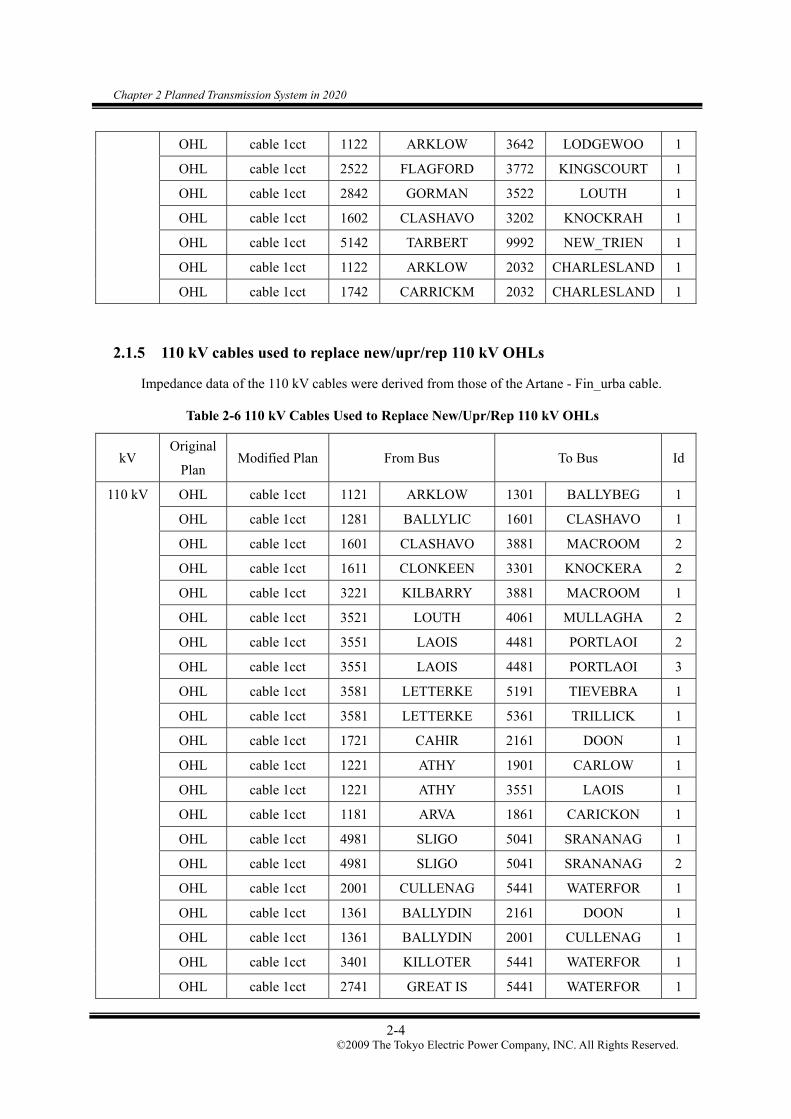
2.1.5 110 kV cables used to replace new/upr/rep 110 kV OHLs
Impedance data of the 110 kV cables were derived from those of the Artane - Fin_urba cable.
Table 2-6 110 kV Cables Used to Replace New/Upr/Rep 110 kV OHLs
kV Original
Plan Modified Plan From Bus To Bus Id
OHL cable 1cct 1121 ARKLOW 1301 BALLYBEG 1
OHL cable 1cct 1281 BALLYLIC 1601 CLASHAVO 1
OHL cable 1cct 1601 CLASHAVO 3881 MACROOM 2
OHL cable 1cct 1611 CLONKEEN 3301 KNOCKERA 2
OHL cable 1cct 3221 KILBARRY 3881 MACROOM 1
OHL cable 1cct 3521 LOUTH 4061 MULLAGHA 2
OHL cable 1cct 3551 LAOIS 4481 PORTLAOI 2
OHL cable 1cct 3551 LAOIS 4481 PORTLAOI 3
OHL cable 1cct 3581 LETTERKE 5191 TIEVEBRA 1
OHL cable 1cct 3581 LETTERKE 5361 TRILLICK 1
OHL cable 1cct 1721 CAHIR 2161 DOON 1
OHL cable 1cct 1221 ATHY 1901 CARLOW 1
OHL cable 1cct 1221 ATHY 3551 LAOIS 1
OHL cable 1cct 1181 ARVA 1861 CARICKON 1
OHL cable 1cct 4981 SLIGO 5041 SRANANAG 1
OHL cable 1cct 4981 SLIGO 5041 SRANANAG 2
OHL cable 1cct 2001 CULLENAG 5441 WATERFOR 1
OHL cable 1cct 1361 BALLYDIN 2161 DOON 1
OHL cable 1cct 1361 BALLYDIN 2001 CULLENAG 1
OHL cable 1cct 3401 KILLOTER 5441 WATERFOR 1
110 kV
OHL cable 1cct 2741 GREAT IS 5441 WATERFOR 1

Chapter 2 Planned Transmission System in 2020
2-5 ©2009 The Tokyo Electric Power Company, INC. All Rights Reserved.
OHL cable 1cct 1481 BUTLERST 3401 KILLOTER 1
OHL cable 1cct 2741 GREAT IS 5501 WEXFORD 1
OHL cable 1cct 2741 GREAT IS 5441 WATERFOR 2
OHL cable 1cct 1661 CASTLEBA 1821 CLOON 1
OHL cable 1cct 2521 FLAGFORD 5341 TONROE 1
OHL cable 1cct 1661 CASTLEBA 2281 DALTON 1
OHL cable 1cct 2741 GREAT IS 3441 KILMURRY 1
OHL cable 1cct 2521 FLAGFORD 3501 LANESBOR 1
OHL cable 1cct 1541 BANOGE 1841 CRANE 1
OHL cable 1cct 1901 CARLOW 3341 KELLIS 1
OHL cable 1cct 1901 CARLOW 3341 KELLIS 2
OHL cable 1cct 1481 BUTLERST 2001 CULLENAG 1
OHL cable 1cct 1121 ARKLOW 1541 BANOGE 1
OHL cable 1cct 1641 CASHLA 2361 ENNIS 1
OHL cable 1cct 1621 COOLROE 3061 INISCARR 1
OHL cable 1cct 1661 CASTLEBA 5341 TONROE 1
OHL cable 1cct 1981 CORRACLA 2821 GORTAWEE 1
OHL cable 1cct 3261 KILKENNY 3441 KILMURRY 1
OHL cable 1cct 5301 THURLES 31019 IKERIN T 1
OHL cable 1cct 4941 SHANNONB 31019 IKERIN T 1
OHL cable 1cct 1981 CORRACLA 79016 ENNK_PST 1
OHL cable 1cct 2521 FLAGFORD 4981 SLIGO 1
OHL cable 1cct 1021 ARDNACRU 2121 DRUMLINE 1
OHL cable 1cct 4941 SHANNONB 22419 DALLOW T 1
OHL cable 1cct 1021 ARDNACRU 2361 ENNIS 1
OHL cable 1cct 3261 KILKENNY 3341 KELLIS 1
OHL cable 1cct 5141 TARBERT 5281 TRALEE 1
OHL cable 1cct 1701 CATH_FAL 1981 CORRACLA 1
OHL cable 1cct 1841 CRANE 5501 WEXFORD 1
OHL cable 1cct 4481 PORTLAOI 22419 DALLOW T 1
OHL cable 1cct 3201 KNOCKRAH 3221 KILBARRY 1
OHL cable 1cct 2181 DRYBRIDG 3521 LOUTH 1
OHL cable 1cct 3281 KILLONAN 3541 LIMERICK 2
OHL cable 1cct 3501 LANESBOR 4001 MULLINGA 1
OHL cable 1cct 1141 ATHLONE 4941 SHANNONB 1

Chapter 2 Planned Transmission System in 2020
2-6 ©2009 The Tokyo Electric Power Company, INC. All Rights Reserved.
OHL cable 1cct 1141 ATHLONE 3501 LANESBOR 1
OHL cable 1cct 1181 ARVA 4961 SHANKILL 1
OHL cable 1cct 1841 CRANE 3641 LODGEWOO 1
OHL cable 1cct 3521 LOUTH 3821 MEATH HI 1
OHL cable 1cct 1861 CARICKON 10619 ARIGNA_T 1
OHL cable 1cct 1141 ATHLONE 4941 SHANNONB 2
OHL cable 1cct 3221 KILBARRY 3961 MARINA 1
OHL cable 1cct 1631 CORDERRY 10619 ARIGNA_T 1
OHL cable 1cct 2841 GORMAN 4501 PLATIN 1
OHL cable 1cct 1701 CATH_FAL 5041 SRANANAG 1
OHL cable 1cct 1701 CATH_FAL 5041 SRANANAG 2
OHL cable 1cct 1701 CATH_FAL 1761 CLIFF 1
OHL cable 1cct 2181 DRYBRIDG 2841 GORMAN 1
OHL cable 1cct 1881 CHARLEVI 4021 MALLOW 1
OHL cable 1cct 3281 KILLONAN 3541 LIMERICK 1
OHL cable 1cct 3201 KNOCKRAH 3221 KILBARRY 2
OHL cable 1cct 3221 KILBARRY 3961 MARINA 2
OHL cable 1cct 3551 LAOIS 4481 PORTLAOI 1
OHL cable 1cct 1241 BALLYCUM 3541 LIMERICK 1
OHL cable 1cct 1241 BALLYCUM 3901 MONETEEN 1
OHL cable 1cct 5361 TRILLICK 75510 COOL1- 1
OHL cable 1cct 3581 LETTERKE 89510 STRABANE 2
OHL cable 1cct 3581 LETTERKE 89510 STRABANE 1
OHL cable 1cct 75010 COLE1- 81510 KELS1- 1
OHL cable 1cct 79010 ENNISKIL 87510 OMAH1- 1
OHL cable 1cct 79010 ENNISKIL 87510 OMAH1- 2
OHL cable 1cct 87510 OMAH1- 89510 STRABANE 1
OHL cable 1cct 87510 OMAH1- 89510 STRABANE 2
OHL cable 1cct 1901 CARLOW 3341 KELLIS 2
OHL cable 1cct 1481 BUTLERST 2001 CULLENAG 1
OHL cable 1cct 1121 ARKLOW 1541 BANOGE 1
OHL cable 1cct 1641 CASHLA 2361 ENNIS 1
OHL cable 1cct 1621 COOLROE 3061 INISCARR 1
OHL cable 1cct 1661 CASTLEBA 5341 TONROE 1
OHL cable 1cct 1981 CORRACLA 2821 GORTAWEE 1

Chapter 2 Planned Transmission System in 2020
2-7 ©2009 The Tokyo Electric Power Company, INC. All Rights Reserved.
OHL cable 1cct 3261 KILKENNY 3441 KILMURRY 1
OHL cable 1cct 5301 THURLES 31019 IKERIN T 1
OHL cable 1cct 4941 SHANNONB 31019 IKERIN T 1
OHL cable 1cct 1981 CORRACLA 79016 ENNK_PST 1
OHL cable 1cct 2521 FLAGFORD 4981 SLIGO 1
OHL cable 1cct 1021 ARDNACRU 2121 DRUMLINE 1
OHL cable 1cct 4941 SHANNONB 22419 DALLOW T 1
OHL cable 1cct 1021 ARDNACRU 2361 ENNIS 1
OHL cable 1cct 3261 KILKENNY 3341 KELLIS 1
OHL cable 1cct 5141 TARBERT 5281 TRALEE 1
OHL cable 1cct 1701 CATH_FAL 1981 CORRACLA 1
OHL cable 1cct 1841 CRANE 5501 WEXFORD 1
OHL cable 1cct 4481 PORTLAOI 22419 DALLOW T 1
OHL cable 1cct 3201 KNOCKRAH 3221 KILBARRY 1
OHL cable 1cct 2181 DRYBRIDG 3521 LOUTH 1
OHL cable 1cct 3281 KILLONAN 3541 LIMERICK 2
OHL cable 1cct 3501 LANESBOR 4001 MULLINGA 1
OHL cable 1cct 1141 ATHLONE 4941 SHANNONB 1
OHL cable 1cct 1141 ATHLONE 3501 LANESBOR 1
OHL cable 1cct 1181 ARVA 4961 SHANKILL 1
OHL cable 1cct 1841 CRANE 3641 LODGEWOO 1
OHL cable 1cct 3521 LOUTH 3821 MEATH HI 1
OHL cable 1cct 1861 CARICKON 10619 ARIGNA_T 1
OHL cable 1cct 1141 ATHLONE 4941 SHANNONB 2
OHL cable 1cct 1141 ATHLONE 3501 LANESBOR 1
OHL cable 1cct 1181 ARVA 4961 SHANKILL 1
OHL cable 1cct 1841 CRANE 3641 LODGEWOO 1
OHL cable 1cct 3521 LOUTH 3821 MEATH HI 1
OHL cable 1cct 1861 CARICKON 10619 ARIGNA_T 1
OHL cable 1cct 1141 ATHLONE 4941 SHANNONB 2
OHL cable 1cct 3221 KILBARRY 3961 MARINA 1
OHL cable 1cct 1631 CORDERRY 10619 ARIGNA_T 1
OHL cable 1cct 2841 GORMAN 4501 PLATIN 1
OHL cable 1cct 1701 CATH_FAL 5041 SRANANAG 1
OHL cable 1cct 1701 CATH_FAL 5041 SRANANAG 2

Chapter 2 Planned Transmission System in 2020
2-8 ©2009 The Tokyo Electric Power Company, INC. All Rights Reserved.
OHL cable 1cct 1701 CATH_FAL 1761 CLIFF 1
OHL cable 1cct 2181 DRYBRIDG 2841 GORMAN 1
OHL cable 1cct 1881 CHARLEVI 4021 MALLOW 1
OHL cable 1cct 3281 KILLONAN 3541 LIMERICK 1
OHL cable 1cct 3201 KNOCKRAH 3221 KILBARRY 2
OHL cable 1cct 3221 KILBARRY 3961 MARINA 2
OHL cable 1cct 3551 LAOIS 4481 PORTLAOI 1
OHL cable 1cct 1241 BALLYCUM 3541 LIMERICK 1
OHL cable 1cct 1241 BALLYCUM 3901 MONETEEN 1
OHL cable 1cct 5361 TRILLICK 75510 COOL1- 1
OHL cable 1cct 3581 LETTERKE 89510 STRABANE 2
OHL cable 1cct 3581 LETTERKE 89510 STRABANE 1
OHL cable 1cct 75010 COLE1- 81510 KELS1- 1
OHL cable 1cct 79010 ENNISKIL 87510 OMAH1- 1
OHL cable 1cct 79010 ENNISKIL 87510 OMAH1- 2
OHL cable 1cct 87510 OMAH1- 89510 STRABANE 1
OHL cable 1cct 87510 OMAH1- 89510 STRABANE 2

Chapter 2 Planned Transmission System in 2020
2-9 ©2009 The Tokyo Electric Power Company, INC. All Rights Reserved.
Fig. 2.1 Power flow diagram of the modified planned transmission system in the year 2020 in summer off-peak demand (Part 1).

Chapter 2 Planned Transmission System in 2020
2-10 ©2009 The Tokyo Electric Power Company, INC. All Rights Reserved.
Fig. 2.2 Power flow diagram of the modified planned transmission system in the year 2020 in summer off-peak demand (Part 2 and 3).

Chapter 3 Selection of the Cable
3-1 ©2009 The Tokyo Electric Power Company, INC. All Rights Reserved.
Chapter 3 Selection of the Cable
3.1 Examples of EHV XLPE Cables
The Woodland – Kingscourt – Turleenan line is required to carry 1500 MVA as a continuous
rating, in order to facilitate further power transactions between NI and RoI and thus to allow for
further connections of renewable generators to the all-island transmission system.
Table 3-1 shows examples of the EHV XLPE directly buried cables with their transmission
capacities. It can be seen that it is difficult to secure 1500 MVA/cct if the cable is directly buried.
A large conductor size with favorable ground conditions will be required.
Note that EHV cables in Vienna and Milan are a part of the mixed OHL/cable line. Both of
them connect the double circuit cable to a single circuit OHL to balance the transmission capacity
in the cable section and the OHL section.
Table 3-1 Examples of EHV XLPE Directly Buried Cables
Location Year Voltage
[kV]
Length
[km]
Conductor
Size [mm2]CKT
Transmission Capacity
(Winter) [MVA/cct]
Copenhagen 1997
1999 400
22
12 1600
1
1
900
(800)
Jutland
(Denmark) 2004 400
14
(4.5+2.5+7)1200 2 500
Vienna 2005 400 5.2 1200 2 620
(1030 with cooling)
Milan 2006 380 8.4 2000 2 1050
Table 3-2 Examples of EHV XLPE Cables in a Tunnel
Location Year Voltage
[kV]
Length
[km]
Conductor
Size [mm2]CKT
Transmission Capacity
(Winter) [MVA/cct]
Berlin 1998
2000 400
6.3
5.5 1600
2
2
1100
1100
Tokyo 2000 500 39.8 2500 2 900 – 1200
Madrid 2004 400 12.8 2500 2 1720
London 2005 400 20 2500 1 1600

Chapter 3 Selection of the Cable
3-2 ©2009 The Tokyo Electric Power Company, INC. All Rights Reserved.
Table 3-2 shows examples of EHV XLPE cables laid in a tunnel with their transmission
capacities. As shown in the table, transmission capacity of 1500 MVA/cct has been achieved in
Madrid and London.
In Berlin, Madrid, and London, cables are laid with 500 – 600 mm space between phases.
Because of this phase spacing, these EHV cables occupy a large proportion of the space in a tunnel.
This will make it difficult for tunnel installation to achieve a cost advantage over directly buried
cables.
3.2 Transmission Capacity Calculation
3.2.1 Woodland – Kingscourt – Turleenan line
In order to find a cable type and layout which assures transmission capacity of 1500 MVA,
transmission capacity calculation was conducted based on IEC 60287. Since the load factor was
specified as unity as the severest assumption, the cyclic rating was not calculated. (IEC 60853 was
not used.)
Based on the results of the transmission capacity calculation, the following cable types and
layouts were selected for further study. In the table, double circuit was selected as base case, upon
which all subsequent conditions will be studied. Single circuit was selected as optional; only
designated severe cases will be studied with Single circuit.
Table 3-3 Selected Cable Types and Layouts
Double circuit Single circuit
Conductor Al 1400 mm2 Cu 2500 mm2
Buried formation Flat Flat
Phase spacing 500 mm 700 mm
In choosing the cable types and layouts shown in Table 3-3, transmission capacity was
calculated for the various cable types and phase spacings. Fig. 3.1 shows the result of the
transmission capacity calculation for double circuit. With phase spacing of 500 mm, Al 1400 mm2
is a reasonable choice in order to assure transmission capacity of 1500 MVA.

Chapter 3 Selection of the Cable
3-3 ©2009 The Tokyo Electric Power Company, INC. All Rights Reserved.
500
600
700
800
900
1000
1100
1200
200 400 600 800 1000
Space between phases [mm]
Tra
nsm
issi
on C
apac
ity [
MV
A/c
ct]
1000mm2(Cu)
1200mm2(Cu)
1400mm2(Cu)
1600mm2(Cu)
1000mm2(Al)
1200mm2(Al)
1400mm2(Al)
1600mm2(Al)1500MVA/2cct
Fig. 3.1 Result of the transmission capacity calculation for double circuit.
Fig. 3.2 shows the result of the transmission capacity calculation for single circuit. It can be
seen that the conductor size of 3000 mm2 is necessary in order to achieve 1500 MVA/cct. Since
XLPE cables with a conductor size of 3000 mm2 are still under development, however, Cu 2500
mm2 was selected for the study of severe cases.
1100
1200
1300
1400
1500
1600
1700
1800
200 400 600 800 1000
Space between phases [mm]
Tra
nsm
issi
on C
apac
ity [
MV
A/c
ct]
2000mm2(Cu)
2500mm2(Cu)
3000mm2(Cu)
1500MVA/1cct
Fig. 3.2 Result of the transmission capacity calculation for single circuit.

Chapter 3 Selection of the Cable
3-4 ©2009 The Tokyo Electric Power Company, INC. All Rights Reserved.
Even though the single circuit option was studied, it does not reflect the intention of TEPCO to
recommend the single circuit option. It needs to be noted that this line will be the longest EHV
cable line if it is built as the cable line for the whole length. Considering relatively poor
performance of the XLPE cables and their accessories [1], the double circuit option should be
preferred to secure the required reliability. However, the reliability of XLPE technology requires
careful assessment since the preferred joint type is in the process of transition from the extruded
mold joint to the pre-molded joint.
[1] CIGRE Working Group B1.10, TB 379, April 2009, “Update of Service Experience of HV
Underground and Submarine Cable Systems”
The key assumptions adopted in the transmission capacity calculation were provided from the
NIE/EirGrid as follows:
Maximum soil temperature: 15 deg C
Soil thermal resistivity: 1.2 K.m/W
Buried depth: 1.3 m (from ground surface to the cable axis)
Load factor: 1.0
Skin effect coefficient: 1.0 (most pessimistic assumption, for double circuit)
0.25[2] (copper enamelled wire, for single circuit)
Proximity effect coefficient: 0.8 (most pessimistic assumption, for double circuit)
0.15[2] (copper enamelled wire, for single circuit)
[2] These values are given in the CIGRE Working Group B1.03, TB 272, June 2005, “Large
Cross-sections and Composite Screens Design”.

Chapter 3 Selection of the Cable
3-5 ©2009 The Tokyo Electric Power Company, INC. All Rights Reserved.
3.2.2 Standard 400 kV Cable
Standard 400 kV cables were used to replace the new 400 kV OHLs as shown in Table 2-2.
Their required transmission capacity is 1424 MVA. Referring to Fig. 3.2, the following cable
types and layouts were selected in order to secure 1424 MVA/cct.
Table 3-4 Selected Cable Type and Layout for the Standard 400 kV Cable
Standard 400 kV Cable
Conductor Cu 2500 mm2
Number of circuit 1
Buried formation Flat
Phase spacing 700 mm

Chapter 3 Selection of the Cable
3-6 ©2009 The Tokyo Electric Power Company, INC. All Rights Reserved.
3.2.3 Standard 275 kV Cable
Standard 275 kV cables were used to replace new 275 kV OHLs as shown in Table 2-3.
Their required transmission capacity is 710 MVA or 1207 MVA. The transmission capacity
calculation was performed in order to determine the cable type and layout. Fig. 3.3 shows the
result of the calculation. The conditions of the calculation were set to equal to those of the
Woodland – Kingscourt – Turleenan line (double circuit).
400
450
500
550
600
650
700
750
800
200 400 600 800 1000
Space between phases [mm]
Tra
nsm
issi
on C
apac
ity [
MV
A/c
ct]
1000mm2(Cu)
1200mm2(Cu)
1400mm2(Cu)
1600mm2(Cu)
1000mm2(Al)
1200mm2(Al)
1400mm2(Al)
1600mm2(Al)
710MVA/cct
604MVA/cct
Fig. 3.3 Result of the transmission capacity calculation for the standard 275 kV cable.
Based on the results of the calculation, the following cable types and layouts were selected to
replace the new 275 kV OHLs.
Table 3-5 Selected Cable Type and Layout for the Standard 275 kV Cable
1207 MVA route 710 MVA route
Conductor Cu 1200 mm2 Cu 1600 mm2
Number of circuit 2 1
Buried formation Flat Flat
Phase spacing 600 mm 800 mm

Chapter 3 Selection of the Cable
3-7 ©2009 The Tokyo Electric Power Company, INC. All Rights Reserved.
3.3 Impedance Calculation
Impedance and susceptance of 400 kV and 275 kV cables were derived from the following
equations:
]km/[)1( RR p
]km/[10)22
ln2.005.0(
]km/[10))2(
ln4
1(2.0
]m/[)ln4
1(
2
33
33
0
c
c
cp
d
s
r
sss
r
GMRX
]km/mho[10)ln(
2 6
0
0
c
in
rp
d
dB
, where
R: a.c. resistance of conductor at the maximum operating temperature
λ: loss factor for sheath
s: phase spacing of the cable
dc: diameter of conductor
εr: relative permittivity of insulation (2.4)
ε0: permittivity of free space (0.008854 μF/km)]
din: diameter of insulation
dc0: diameter of conductor including conductor screen
Here, R and λ have to be obtained through transmission capacity calculation.
The data applied to the impedance calculation is shown in Table 3-6. Diameters of the 400
kV cables were obtained from Nexan’s specifications. The insulation thickness of the standard
275 kV cable (18.7 mm) were converted from the insulation thickness of 400 kV cables (25.4 mm)
using the proportion of LIWV.
25.4 mm × (1050 kV / 1425 kV) = 18.7 mm

Chapter 3 Selection of the Cable
3-8 ©2009 The Tokyo Electric Power Company, INC. All Rights Reserved.
Table 3-6 Input Data for Impedance Calculation
Woodland – Turleenan line Standard
400 kV CableStandard 275 kV Cable
Conductor Al 1400 mm2 Cu 2500 mm2 Cu 2500 mm2 Cu 1200 mm2 Cu 1600 mm2
Buried
formation Flat Flat Flat Flat Flat
s [mm] 500 700 700 600 800
dc [mm] 45.0 65.2 65.2 41.7 48.2
dc0 [mm] 48.0 68.2 68.2 44.7 51.2
din [mm] 98.8 119.0 119.0 82.1 88.6
R [Ω/m] 3.001×10⁻⁵ 9.722×10⁻⁶ 9.722×10⁻⁶ 2.292×10⁻⁵ 1.880×10⁻⁵
λ 0.05070 0.08324 0.08324 0.04152 0.03972
Based on the results of the calculation, impedance and capacitance of the cables were
determined as follows:
Table 3-7 Impedance and Capacitance of the Selected Cables
Woodland – Turleenan line Standard
400 kV CableStandard 275 kV Cable
Al 1400 mm2 Cu 2500 mm2 Cu 2500 mm2 Cu 1200 mm2 Cu 1600 mm2
Rp [Ω/km] 0.03153 0.01053 0.01053 0.02387 0.01955
Xp [Ω/km] 0.2251 0.2229 0.2229 0.2413 0.2503
C [μF/km] 0.1850 0.2398 0.2398 0.2196 0.2435

Part 1

Part 1:
Evaluation of the Potential Impact on the
All-island Transmission System of Significant
Length of EHV Underground Cable, Either
Individually or in Aggregate Introduction
Table of contents
©2009 The Tokyo Electric Power Company, INC. All Rights Reserved.
Table of contents
CHAPTER 1 INTRODUCTION _________________________________________________ 1-1
CHAPTER 2 REACTIVE POWER COMPENSATION _____________________________ 2-1
2.1 Considerations in Reactive Power Compensation _____________________________ 2-1
2.2 Maximum Unit Size of 400 kV Shunt Reactors _______________________________ 2-2
2.3 Proposed Compensation Patterns __________________________________________ 2-7
2.4 Voltage Profile under Normal Operating Conditions ___________________________ 2-8
2.5 Ferranti Phenomenon ___________________________________________________ 2-9
2.6 Conclusion __________________________________________________________ 2-13
CHAPTER 3 MODEL SETUP __________________________________________________ 3-1
3.1 Modeled Area for This Project ____________________________________________ 3-1
3.2 Transformers __________________________________________________________ 3-1
3.3 Shunt Reactors ________________________________________________________ 3-1
CHAPTER 4 TEMPORARY OVERVOLTAGE ANALYSIS __________________________ 4-1
4.1 Series Resonance Overvoltage ____________________________________________ 4-1
4.2 Parallel Resonance Overvoltage ___________________________________________ 4-1
4.3 Overvoltage Caused by the System Islanding_________________________________ 4-1
4.4 Conclusion ___________________________________________________________ 4-1
CHAPTER 5 SLOW-FRONT OVERVOLTAGE ANALYSIS _________________________ 5-1
5.1 Overvoltage Caused by Line Energisation ___________________________________ 5-1
5.2 Ground Fault and Fault Clearing Overvoltage ________________________________ 5-1
5.3 Conclusion ___________________________________________________________ 5-1
CHAPTER 6 VOLTAGE STABILITY / VARIATION _______________________________ 6-1
6.1 Voltage Variation by the Loss of the 400 kV Cable ____________________________ 6-1
6.2 Voltage Stability with the Loss of the 400 kV Cable ___________________________ 6-1
6.3 Conclusion ___________________________________________________________ 6-1
CHAPTER 7 BLACK-START CAPABILITY______________________________________ 7-1
7.1 Restoration in the Eirgrid Network_________________________________________ 7-1
7.2 Restoration in the NIE Network ___________________________________________ 7-1
7.3 Conclusion ___________________________________________________________ 7-1

Chapter 1 Introduction
1-1 ©2009 The Tokyo Electric Power Company, INC. All Rights Reserved.
Chapter 1 Introduction
The objective of Part 1 is to evaluate the potential impact on the all-island transmission system
of significant lengths of EHV underground cables. In order to fulfill this objective, the following
studies were performed:
(1) Transmission Capacity Calculation
(2) Impedance and Admittance Calculation
(3) Reactive Power Compensation Analysis
(4) Overvoltage Analysis
(5) Voltage Stability and Variation Analysis
(6) Black-start Studies
Here, (1) and (2) have already been conducted as a common study for Part 1, 2, and 3 and are
not included in this Part 1 report. Using cable information, such as cable size, type, layout, and
impedance / admittance, found in (1) and (2), the remaining studies (3) – (6) were conducted as
Part 1 studies.
The purpose of (3) is to find shunt reactors that should be installed together with the 400 kV
cable. The best combination in terms of the number of shunt reactors, shunt reactor size, and
location was found from (3).
The studies (4) – (6) are to look into the potential adverse effects caused by significant lengths
of EHV underground cables. Temporary overvoltage analysis in the study (4) addresses the most
important concern due to significant lengths of EHV underground cables. In order to set the most
severe condition in (4), the 400 kV Kilkenny – Cahir – Aghada line was selected as the focus of the
study except for the series resonance overvoltage analysis. The 400 kV Kilkenny – Cahir –
Aghada line was selected since it was the longest 400 kV line in the weakest part of the network in
the planned transmission system for the year 2020. The series resonance overvoltage analysis
focused on the 400 kV Woodland – Kingscourt – Turleenan line because of possible large cable
capacitance generated in the 220 kV Woodland / Kingscourt network and the 275 kV Turleenan
network.
Although the objective of Part 1 to evaluate the potential impact on the all-island transmission
system of significant lengths of EHV underground cables, it is not possible to evaluate all possible
scenarios or to choose one severest case. The study instead focused on the reasonable worst-case
scenario in terms of the feasibility. For the installation of a particular cable line, more work has to
be done for the cable line.

Chapter 2 Reactive Power Compensation
2-1 ©2009 The Tokyo Electric Power Company, INC. All Rights Reserved.
Chapter 2 Reactive Power Compensation
2.1 Considerations in Reactive Power Compensation
Shunt reactors are often installed with long cable lengths to compensate for the reactive power
generated with these cables. A compensation rate of close to 100% is preferable as the cable
installation does not change the voltage profile of the network. However it may lead to a severe
zero-miss phenomenon. The effect of the compensation rate is summarized in Table 2-1.
Table 2-1 Effect of Compensation Rate
Analyses Close to 100% Away from 100%
Reactive power compensation Preferable
Generally not preferable
(depends on typical operating
conditions)
Zero-miss phenomenon
Not preferable
(but can be avoided by a
special relay)
Preferable
Oscillatory overvoltage Preferable Not preferable
Zero-miss phenomenon and associated equipment failure can be avoided by installing the
special relay or operational countermeasures. If it is permissible to adopt thes relays or
countermeasures, it is preferable to have a compensation rate close to 100%.
Additionally, the location of shunt reactors must be taken into consideration. Shunt reactors
are connected directly to the cable, to the substation bus, or to the tertiary side of a transformer.
The advantages and disadvantages of these options are described in Table 2-2.
Table 2-2 Installed Location of Shunt Reactors
Connection Advantage Disadvantage
Directly connected to the
cable
- Can limit the overvoltage
when one side of the cable is
opened
- Cannot be used for voltage
control when the cable is
not-in-service (some exceptions
exist.)
Substation bus or tertiary
side of a transformer
- Can be shared by multiple
cable routes
- Cheaper (tertiary side)
- May cause reactive power
imbalance during switching
operations

Chapter 2 Reactive Power Compensation
2-2 ©2009 The Tokyo Electric Power Company, INC. All Rights Reserved.
For extended cable systems such as the 400 kV Woodland – Kingscourt – Turleenan line,
shunt reactors should be directly connected to the cables to control overvoltage when one side of
the cable is opened.
2.2 Maximum Unit Size of 400 kV Shunt Reactors
In Part 1, the 400 kV Kilkenny – Cahir – Aghada line was selected to be the focus of the study
except for the series resonance overvoltage analysis. The Kilkenny – Cahir – Aghada line was
considered to have the most critical conditions due to the long length of the line and small fault
current level around the line. For the series resonance analysis, the 400 kV Woodland –
Kingscourt – Turleenan line was selected to be the focus of the study since it was necessary to have
a large amount of cables on the secondary side in order to have low series resonance frequency.
In this chapter in Part 1, the reactive power compensation of the 400 kV Kilkenny – Cahir –
Aghada line was studied. The reactive power compensation analysis of the 400 kV Woodland –
Kingscourt – Turleenan line is described in Chapter 1 of the Part 2 report.
First, the maximum unit size of 400 kV shunt reactors have been determined from a voltage
variation when one unit of these shunt reactors was switched. The following voltage variation is
allowed in the operation of the all-island transmission system.
Under normal operating conditions: 3 % (11.4 kV)
Under contingencies: 10 % (38.0 kV)
Note that the power flow data provided from the NIE/EirGrid uses a nominal voltage of 380
kV. In this report, however, all the values are calculated based on the nominal voltage 400 kV
(equivalent to 1 pu).
The voltage variation increases under lower load conditions. Power flow data during
summer off-peak demand was selected to allow the analysis of this voltage variation. Shunt
reactors of different sizes were switched on and off at the Kilkenny 400 kV bus. Fig. 2-1 shows
the voltage variation at the buses near Kilkenny 400 kV.

Chapter 2 Reactive Power Compensation
2-3 ©2009 The Tokyo Electric Power Company, INC. All Rights Reserved.
0
0.01
0.02
0.03
0.04
0.05
0 50 100 150
Unit Size of Shunt Reactor [MVA]
Vol
tage
Var
iatio
n [p
u
KILKENNY 220
KILKENNY 400
CAHIR 400
AGHADA 400
AGHADA 220
Fig. 2-1 Voltage variation with shunt reactor switchings at the Kilkenny 400 kV bus.
From Fig. 2-1, it can be seen that the maximum unit size which can be installed to the
Kilkenny 400 kV bus is 100 MVA. The same limitation can be applied when the shunt reactor is
directly connected to the cable near the Kilkenny 400 kV bus.

Chapter 2 Reactive Power Compensation
2-4 ©2009 The Tokyo Electric Power Company, INC. All Rights Reserved.
The same analysis was performed with shunt reactors connected to the Cahir 400 kV bus.
The result of the analysis is shown in Fig. 2-2.
0
0.01
0.02
0.03
0.04
0.05
0 50 100 150
Unit Size of Shunt Reactor [MVA]
Vol
tage
Var
iatio
n [p
u
KILKENNY 220
KILKENNY 400
CAHIR 400
AGHADA 400
AGHADA 220
Fig. 2-2 Voltage variation with shunt reactor switchings at the Cahir 400 kV bus.
It can be seen that the maximum unit size which can be installed to the Cahir 400 kV bus is
100 MVA. The same limitation can be applied when the shunt reactor is directly connected to the
cable near the Cahir 400 kV bus.

Chapter 2 Reactive Power Compensation
2-5 ©2009 The Tokyo Electric Power Company, INC. All Rights Reserved.
0
0.01
0.02
0.03
0.04
0.05
0.06
0 50 100 150
Unit Size of Shunt Reactor [MVA]
Vol
tage
Var
iatio
n [p
u
KILKENNY 220
KILKENNY 400
CAHIR 400
AGHADA 400
AGHADA 220
Fig. 2-3 Voltage variation with shunt reactor switchings at the Aghada 400 kV bus.
Fig. 2-3 shows the result of the same analysis for the Aghada 400 kV bus. The 400 kV bus
voltage of Aghada is less stable than that of Cahir. It can be seen that the maximum unit size
which can be installed to the Cahir 400 kV bus is 80 MVA. The same limitation can be applied
when the shunt reactor is directly connected to the cable near the Aghada 400 kV bus.

Chapter 2 Reactive Power Compensation
2-6 ©2009 The Tokyo Electric Power Company, INC. All Rights Reserved.
0
0.01
0.02
0.03
0.04
0.05
0 50 100 150
Unit Size of Shunt Reactor [MVA]
Vol
tage
Var
iatio
n [p
u
KILKENNY 220
KILKENNY 400
CAHIR 400
AGHADA 400
AGHADA 220
Fig. 2-4 Voltage variation with shunt reactor switchings at the shunt station.
Fig. 2-4 shows the voltage variation when a 400 kV shunt reactor is switched on/off at a shunt
reactor station located at the center of the 400 kV Cahir – Aghada line. It can be seen that the
maximum unit size which can be installed at the shunt reactor station is 100 MVA.

Chapter 2 Reactive Power Compensation
2-7 ©2009 The Tokyo Electric Power Company, INC. All Rights Reserved.
2.3 Proposed Compensation Patterns
Charging capacity of the Kilkenny – Cahir – Aghada line is:
Kilkenny – Cahir: 723.3 MVA @ 400 kV
Cahir – Aghada: 1350.2 MVA @ 400 kV
Based on the maximum unit size found in the previous section, the following reactive power
compensation patterns were proposed:
Table 2-3 Proposed Compensation Patterns
For the 400 kV Kilkenny – Cahir cable:
Locations Case A
Kilkenny
Cahir
100 MVA × 4
80 MVA × 4
Compensation
Rate [%] 99.5
For the 400 kV Cahir – Aghada cable:
Locations Case B1 Case B2 Case B3
Cahir
Station
Aghada
100 MVA × 4
80 MVA × 8
80 MVA × 4
100 MVA × 4
80 MVA × 7
80 MVA × 5
80 MVA × 4
80 MVA × 8
80 MVA × 5
Compensation
Rate [%] 100.7 100.7 100.7
Case B1,B2 and B3 consider the shunt reactor station at the center of the Cahir – Aghada line.

Chapter 2 Reactive Power Compensation
2-8 ©2009 The Tokyo Electric Power Company, INC. All Rights Reserved.
2.4 Voltage Profile under Normal Operating Conditions
From the reactive power compensation analysis, a simple power flow data for the Kilkenny –
Cahir – Aghada line was constructed. In this simple model, both the Kilkenny – Cahir line and the
Cahir – Aghada line were divided into six sections of equal length, in order to observe the voltage
profile along the line and to model shunt reactor stations.
The following conditions were assumed in the power flow data:
The 400 kV bus voltages of Kilkenny and Aghada are maintained below 410 kV. As
the most severe condition, these bus voltages are fixed to 410 kV.
The power flow model created for the reactive power compensation analysis is shown in Fig.
2-5.
Fig. 2-5 Power flow model for the reactive power compensation analysis.
Using this power flow model, the voltage profile along the line was initially considered with
all the equipment in service. The analysis was performed under no load conditions.
The results of the analysis are shown in Fig. 2-6. The voltage rise at the center of the line
peaks at 4 kV. Considering the highest voltage (420 kV) of equipment, all compensation patterns
have a satisfactory voltage profile.

Chapter 2 Reactive Power Compensation
2-9 ©2009 The Tokyo Electric Power Company, INC. All Rights Reserved.
406
408
410
412
414
416
418
420K
ILK
EN
NY T1
T2
T3
T4
T5
CA
HIR T
6
T7
T8
T9
T10
AG
HA
DA
case B1
case B2
case B3
Fig. 2-6 Voltage profile in the normal operating condition (no load).
2.5 Ferranti Phenomenon
When one end of the line is opened due to a switching operation or a bus fault, the voltage at
the open terminal may rise due to charging current. Although equipment failure caused by this
overvoltage can be prevented by opening the other end of the line, this overvoltage can be
overlooked since the voltage at the open terminal is not monitored. From a planning standpoint, it
is recommended to maintain the voltage at the open terminal below 420 kV in order to relieve
operational concerns.
2.5.1 Shunt Reactors Connected to the Line
First, the voltage profile when all shunt reactors were directly connected to the line was
studied. When connected to the line, shunt reactors can be used to suppress the open terminal
voltage.
Fig. 2-7 shows the voltage profile when the Aghada terminal is opened. The different
compensation patterns Case B1 – B3 were studied for the Cahir – Aghada line. The compensation
pattern of the Cahir – Aghada line was fixed to Case B3, and the Kilkenny 400 kV bus voltage was
fixed at 410 kV. It appears that all compensation patterns have a satisfactory voltage profile.

Chapter 2 Reactive Power Compensation
2-10 ©2009 The Tokyo Electric Power Company, INC. All Rights Reserved.
406
408
410
412
414
416
418
420
KIL
KE
NN
Y T1
T2
T3
T4
T5
CA
HIR T
6
T7
T8
T9
T10
AG
HA
DA
Case B1
Case B2
Case B3
Fig. 2-7 Voltage profile when the Aghada terminal is opened.
Fig. 2-8 shows the voltage profile when the Kilkenny terminal is opened. The different
compensation patterns Case B1 – B3 were studied for the Cahir – Aghada line. The Aghada 400
kV bus voltage was fixed at 410 kV. It can be seen that all compensation patterns have a
satisfactory voltage profile.
406
408
410
412
414
416
418
420
KIL
KE
NN
Y T1
T2
T3
T4
T5
CA
HIR T6
T7
T8
T9
T10
AG
HA
DA
Case B1
Case B2
Case B3
Fig. 2-8 Voltage profile when the Kilkenny terminal is opened.

Chapter 2 Reactive Power Compensation
2-11 ©2009 The Tokyo Electric Power Company, INC. All Rights Reserved.
2.5.2 Shunt Reactors Connected to the Bus
Shunt reactors connected to the bus is often preferred, compared to those connected to the line,
because of increased flexibility for wider use as voltage and reactive power control equipment.
When considering the Ferranti phenomenon, bus-connected shunt reactors present more severe
conditions as they can not be used to suppress open terminal voltage.
When shunt reactors are connected to the line, they will suppress the open terminal voltage as
long as they are available. When line-connected shunt reactors are not available, for example due
to maintenance outage, the condition becomes similar to bus-connected shunt reactors.
Fig. 2-9 shows the voltage profile when the Aghada terminal is opened. All conditions are
identical to those in Section 2.5.1, but 1 unit of the shunt reactors at the Aghada open terminal has
been disconnected. It can be seen from the figure that Case B3 has a satisfactory voltage profile.
In Cases B1 and B2, the voltage along the Cahir – Aghada line exceeds 420 kV, but the voltage rise
from Cahir is within 10 kV. If the Cahir 400 kV bus voltage is maintained below 410 kV, the open
terminal voltage will be maintained below 420 kV.
408
410
412
414
416
418
420
422
424
KIL
KE
NN
Y T1
T2
T3
T4
T5
CA
HIR T
6
T7
T8
T9
T10
AG
HA
DA
Case B1
Case B2
Case B3
Fig. 2-9 Voltage profile when the Aghada terminal is opened without one unit of shunt
reactors.

Chapter 2 Reactive Power Compensation
2-12 ©2009 The Tokyo Electric Power Company, INC. All Rights Reserved.
Fig. 2-10 shows the voltage profile when the Kilkenny terminal is opened. All conditions are
identical to those in Section 2.5.1, but one unit of shunt reactors at the Kilkenny open terminal has
been disconnected. It can be seen from the figure that Case B1 has a satisfactory voltage profile.
In Cases B2 and B3, the voltage along the Kilkenny – Cahir line exceeds 420 kV, but the voltage
rise from Cahir is within 10 kV. If the Cahir 400 kV bus voltage is maintained below 410 kV, the
open terminal voltage will be maintained below 420 kV.
408
410
412
414
416
418
420
422
424
KIL
KE
NN
Y T1
T2
T3
T4
T5
CA
HIR T6
T7
T8
T9
T10
AG
HA
DA
Case B1
Case B2
Case B3
Fig. 2-10 Voltage profile when the Kilkenny terminal is opened without one unit of shunt
reactors.

Chapter 2 Reactive Power Compensation
2-13 ©2009 The Tokyo Electric Power Company, INC. All Rights Reserved.
2.6 Conclusion
As a result of the reactive power compensation analysis, compensation patterns A and B2 were
selected for further analysis.
Locations Case A
Kilkenny
Cahir
100 MVA × 4
80 MVA × 4
Compensation
Rate [%] 99.5
For the 400 kV Cahir – Aghada cable, Cases B1-B3 have a satisfactory voltage profile when
all shunt reactors are connected to the line. When one unit of shunt reactors at the open terminal are
disconnected, the open terminal voltage exceeds 420 kV in all compensation patterns, but the
voltage rise from Cahir is within 10 kV. If the Cahir 400 kV bus voltage is maintained below 410
kV, the open terminal voltage will be maintained below 420 kV.
Case B2 is selected because of its more preferable voltage profile when one unit of shunt
reactors at the open terminal has been disconnected.
Locations Case B1 Case B2 Case B3
Cahir
Station
Aghada
100 MVA × 4
80 MVA × 8
80 MVA × 4
100 MVA × 4
80 MVA × 7
80 MVA × 5
80 MVA × 4
80 MVA × 8
80 MVA × 5
Compensation
Rate [%] 100.7 100.7 100.7
Note: If it is not necessary to switch these shunt reactors for the voltage and reactive power control,
it is possible to choose a shunt reactor of larger unit size. For example in Case B2, it is
possible to install two units of 200 MVA shunt reactors in Cahir instead of four units of 100
MVA. The compensation pattern in Case B2 was selected without the consideration of the
requirements for the voltage and reactive power control, since it is not included in the scope
of this study and the difference can have only small effects on the simulation results.

Chapter 2 Reactive Power Compensation
2-14 ©2009 The Tokyo Electric Power Company, INC. All Rights Reserved.
When a shunt reactor with large unit size is selected, an outage of this shunt reactor will
significantly lower the compensation rate of the cable line, which may prohibit the use of the
line during the outage.

Chapter 3 Model Setup
3-1 ©2009 The Tokyo Electric Power Company, INC. All Rights Reserved.
Chapter 3 Model Setup
3.1 Modeled Area for This Project
In Part 1, the 400 kV Kilkenny – Cahir – Aghada line was selected to be the focus of the study
except for the series resonance overvoltage analysis as mentioned in Chapter 1. The figure below
shows an example of the model created by ATP-Draw.
56kmX0034 X0044
GROUPagh-chr
X0095
CH4T1
KLKN4
X0095
I
X0095
AGHD4 KLKN2
V
AGH4T AGH2T
Y Y
I-Phi
VV
X0044
AGHD2
V
31mH
X0096
50mH
X0097
CH1T1Y Y
I-Phi CH1T1
X0175
KLK4T KLK2T
Y Y
I-Phi
15mH
X0107
60kmX0108 X0128
GROUPkel-lao
0.0L 0.0
V
V
V
VV
V V
V V
0.0L 0.0
V
Y Y
ABC
Fig. 3-1 Simulation model for the temporary overvoltage and slow-front overvoltage analysis.
For the series resonance analysis, the 400 kV Woodland – Kingscourt – Turleenan line was
selected to be the focus of the study. Since the Part 2 study focused on the 400 kV Woodland –
Kingscourt – Turleenan line, simulation models for the series resonance analysis were introduced in
the Part 2 report.
For the series resonance overvoltage analysis, it is necessary to model the 275 kV and 220 kV
network. The 275 kV and 220 kV networks around Woodland, Kingscourt, and Turleenan were
included in the model by distributed parameter models, whose input data were derived from PSS/E
powerflow data.
Aghada – Cahir line Cahir – Kilkenny line

Chapter 3 Model Setup
3-2 ©2009 The Tokyo Electric Power Company, INC. All Rights Reserved.
3.2 Transformers
Model parameters of the Kingscourt 400/220 kV transformer were provided from NIE/EirGrid.
These parameters are shown in Table 3-1. Aghada and Kilkenny 400/220 kV transformers in the
RoI were assumed to have the same parameters as the Kingscourt 400/220 kV transformer.
Model parameters of the Cahir 400/110 kV transformer were derived from PSS/E power flow
data.
Table 3-1 Model Parameters of the Kingscourt 400/220 kV Transformer
For leakage inductances in Table 3-1, percent impedances were converted to mH by the
following calculations.
(x%1-2, x%1-3, x%2-3) → (x%1, x%2, x%3)
232%31%21%
1%
xxx
x
231%3221%
2%
xxx
x
221%32%31%
3%
xxx
x
(x%1, x%2, x%3) → (x1, x2, x3)
1000502
1
MVA100
)kV400(
100
21%
1
xx [mH]
1000502
1
MVA100
)220kVor 275(
100
22%
2
xx [mH]
1000502
1
MVA100
)21kVor 33(
100
23%
3
xx [mH]

Chapter 3 Model Setup
3-3 ©2009 The Tokyo Electric Power Company, INC. All Rights Reserved.
Internal resistance and leakage inductance of these transformers were obtained as follows:
Substations R1 [Ω] X1 [mH] R2 [Ω] X2 [mH] R3 [Ω] X3 [mH]
Aghada
Kilkenny 0.3719 137.10 0.1793 0.001 0.035430 1.8812
Cahir 0.0001 273.49 0.0581 4.814 0.002481 0.0790
Saturation characteristic of a 400/275/13 kV 750 MVA transformer in National Grid was
provided from NIE/EirGrid as shown in Table 3-2. The same saturation characteristic was
assumed for the Cahir 400/110 kV transformer.
Table 3-2 Saturation Characteristic of the 400 kV Transformer (defined in tertiary)
I [A] Phi [Wb-T]
51.63578 2.30940
55.07817 5.35781
58.52055 9.79186
61.96294 21.70836
65.40533 61.43004
68.84771 187.06140
72.29010 424.92960
82.61725 6267.24695

Chapter 3 Model Setup
3-4 ©2009 The Tokyo Electric Power Company, INC. All Rights Reserved.
For transformer inrush studies, the magnetizing branch hysteresis curve was derived from the
saturation characteristic in Table 3-2 using the subroutine HYSDAT. The lower half of the
obtained hysteresis curve is shown in Table 3-3.
Table 3-3 Hysteresis Curve of the 400 kV Transformer (defined in primary)
I [A] Phi [Wb-T]
-29.4000 -1424.49
-3.6750 -1349.38
2.2050 -1243.19
5.1450 -966.929
9.9225 837.430
15.4350 1105.06
26.4600 1269.09
48.8775 1381.33
117.6000 1467.66
161.7000 1476.29

Chapter 3 Model Setup
3-5 ©2009 The Tokyo Electric Power Company, INC. All Rights Reserved.
3.3 Shunt Reactors
3.3.1 400 kV Shunt Reactor
Shunt reactors were connected to both ends of the 400 kV cables or 400 kV buses, in order to
compensate charging capacity of the cables. Only for the Kingscourt – Turleenan line and the
Kilkenny – Aghada line, shunt reactors were also connected to the center of the line. Shunt
reactors for the Kilkenny – Cahir – Aghada line were modeled based on the result of the analysis in
Chapter 1. 400 kV shunt reactors in the simulation model are shown in Table 3-4.
Table 3-4 400 kV Shunt Reactors in the Simulation Model
From Bus To Bus Length
[km]
From
[MVA]
Centre
[MVA]
To
[MVA]
3774 KINGSCOURT 5464 WOODLAND 58 120× 2 - 150× 2
3774 KINGSCOURT 5464 WOODLAND 58 120× 2 - 150× 2
3774 KINGSCOURT 90140 TURL 82 100× 2 120× 3 100× 2
3774 KINGSCOURT 90140 TURL 82 100× 2 120× 3 100× 2
1044 AGHADA 1724 CAHIR 112 80× 5 80× 7 100× 4
1124 ARKLOW 2744 GREAT_ISL 60 180× 2 - 180× 2
1724 CAHIR 3264 KILKENNY 60 80× 4 - 100× 4
2524 FLAGFORD 3774 CAVAN 60 180× 2 - 180× 2
3344 KELLIS 3554 LAOIS 60 180× 2 - 180× 2
2204 DUNSTOWN 3854 MAYNOOTH 30.55 180× 1 - 180× 1
3854 MAYNOOTH 5464 WOODLAND 22.5 150× 1 - 150× 1
When 400 kV shunt reactors are close to the point of interest, they are modeled with the
saturation characteristic. Otherwise, they are modeled as linear inductances.

Chapter 3 Model Setup
3-6 ©2009 The Tokyo Electric Power Company, INC. All Rights Reserved.
3.3.2 275 kV Shunt Reactor
Shunt reactors were connected to both ends of 275 kV cables in order to compensate charging
capacity of the cables. Shunt reactors connected to the 275 kV cables in the simulation model are
shown in Table 3-5.
Table 3-5 Shunt Reactors Connected to Both Ends of 275 kV Cables in the Simulation Model
From Bus To Bus Length[km]From
[MVA]
To
[MVA]
87520 OMAH 90120 TURL 42 100 100
87520 OMAH 90120 TURL 42 100 100
87520 OMAH 90120 TURL 42 100 100
87520 OMAH 90120 TURL 42 100 100
87520 OMAH 89520 STRABANE 60 160 160
87520 OMAH 89520 STRABANE 60 160 160
75520 COOLKEER 89520 STRABANE 25 60 60
75520 COOLKEER 89520 STRABANE 25 60 60
Shunt reactors were connected to 275 kV buses in order to compensate charging capacity of
the short 110 kV cables. Shunt reactors connected to 275 kV buses in the simulation model are
shown in Table 3-6.
Table 3-6 Shunt Reactors connected to 275 kV buses in the Simulation Model
Shunt reactor [MVA]
kV Bus
number Bus name Winter_peak_
wind_maximum
Summer_
off_peak
75520 COOLKEER 100 100
87520 OMAH 100 100 275
89520 STRABANE 100 100

Chapter 3 Model Setup
3-7 ©2009 The Tokyo Electric Power Company, INC. All Rights Reserved.
3.3.3 220 kV Shunt Reactor
Shunt reactors were connected to both ends of long 220 kV cables in order to compensate
charging capacity of the cables. Shunt reactors connected to the 220 kV cables in the simulation
model are shown in Table 3-7.
Table 3-7 Shunt Reactors Connected to Both Ends of 220 kV Cables in the Simulation Model
From Bus To Bus Length
[km]
From
[MVA]
To
[MVA]
1402 BELLACOR 2522 FLAGFORD 123 160 160
1642 CASHLA 4522 PROSPECT 90 120 120
4942 SHANNONB 5492 WMD_220 70 100 100
2522 FLAGFORD 3772 CAVAN 90 120 120
Shunt reactors were connected to 220 kV buses in order to compensate charging capacity of
the 110 kV and short 220 kV cables. Shunt reactors were connected to the 220 kV buses in order
to meet the following conditions:
- Voltage profile of the 220 kV network in the modified data is nearly equal to that of
the original data.
- Unit size of shunt reactor is greater than 100 MVA.

Chapter 3 Model Setup
3-8 ©2009 The Tokyo Electric Power Company, INC. All Rights Reserved.
Shunt reactors connected to 220 kV buses in the simulation model are shown in Table 3-8.
Table 3-8 Shunt Reactors Connected to 220 kV Buses in the Simulation Model
Shunt reactor [MVA]
KV Bus
number Bus name Winter peak
wind_maximum
Summer
off_peak
1122 ARKLOW 250 250
1432 BALLYRAGGET 100 100
1602 CLASHAVO 100 100
1642 CASHLA - 150
2002 CULLENAG 100 100
2032 CHARLESLAND 100 100
2042 CORDUFF 100 100
2202 DUNSTOWN 100 100
2522 FLAGFORD 100 100
2742 GREAT IS - 100
2842 GORMAN - 200
3202 KNOCKRAH - 100
3282 KILLONAN 100 100
3342 KELLIS 100 100
3522 LOUTH 200 200
3552 LAOIS 100 100
3642 LODGEWOO 150 150
4942 SHANNONB 100 100
4952 KINNEGAD-220 100 200
5042 SRANANAG - 100
5142 TARBERT 100 100
5462 WOODLAND - 100
220
9992 NEW_TRIEN 100 100

Chapter 3 Model Setup
3-9 ©2009 The Tokyo Electric Power Company, INC. All Rights Reserved.
Note: Other sections of this capter have been removed from this public report.

Chapter 4 Temporary Overvoltage Analysis
4-1 ©2009 The Tokyo Electric Power Company, INC. All Rights Reserved.
Chapter 4 Temporary Overvoltage Analysis
For long EHV cables, temporary overvoltages are of highest concerns in terms of the safe
operation after the installation. Highest temporary overvoltages are often higher than highest
slow-front overvoltages.
Due to the large capacitance associated with the long EHV cable and the inductance of shunt
reactors for the reactive power compensation, the following temporary overvoltages require a close
attention for the network with long EHV cables. The theoretical backgrounds relating the large
capacitance and the inductance to these temporary overvoltages are given in the beginning of each
section:
(1) Series resonance overvoltage
(2) Parallel resonance overvoltage
(3) Oscillatory overvoltage caused by the system islanding
For equipment whose highest voltage is lower than or equal to 245 kV, the standard
short-duration power-frequency withstand voltage is specified in IEC 71-1. The series resonance
overvoltage analysis in the Woodland and Kingston 220 kV network evaluates the overvoltage level
against the standard short-duration power-frequency withstand voltage.
For equipment whose highest voltage is higher than 245 kV, the standard short-duration
power-frequency withstand voltage is not specified in IEC, but it is specified by a utility or a
manufacturer. Surge arresters are generally the weakest among different equipment. The
temporary overvoltages have to be evaluated against typical withstand voltage and energy
absorption capability of surge arresters. Note that the temporary overvoltages may be evaluated
with SIWV depending on their decay time.

Chapter 4 Temporary Overvoltage Analysis
4-2 ©2009 The Tokyo Electric Power Company, INC. All Rights Reserved.
4.1 Series Resonance Overvoltage
For the series resonance overvoltage analysis, it is necessary to model its 275/220 kV network.
The 275/220 kV networks of target substations were included in the model by distributed parameter
models, whose input data were derived from PSS/E powerflow data.
Series resonance caused by the energisation of each route from both directions was studied.
The switching scenarios are shown below. Before the time domain analysis, frequency scan was
performed for the energised line as well as the combination of 400/275/220 kV transformers and
the 275/220 kV network. The frequency of the overvoltage caused by the energisation and the
resonance frequency of the 275/220 kV network can be found from the result of frequency scan,
and it is possible to assess the chance of having series resonance. After the frequency scan, the
series resonance overvoltage analysis was conducted under the following two conditions with
time-domain simulation:
(1) Normal condition where all 400/275/220 kV transformers and 275/220 kV lines in
Woodland, Kingscourt, and Turleenan are in service
(2) Assumed most severe condition where the frequency of the overvoltage is closest to the
resonance frequency of the 275/220 kV network

Chapter 4 Temporary Overvoltage Analysis
4-3 ©2009 The Tokyo Electric Power Company, INC. All Rights Reserved.
Woodland 220 kV system
Turleenan Kingscourt Woodland
On
MNYPGCoolkeeragh
Omagh
Flagford
Turleenan275kV
Turleenan 275 kV
…
Kingscourt 220 kV system (Closing of Turleenan side)
Kingscourt 220 kV system (Closing of Woodland side)
Fig. 4-1 Switching scenarios for the series resonance overvoltage analysis.
Close
Open
On
Close
Open
On
Close
Open
On
Close
Open
On

Chapter 4 Temporary Overvoltage Analysis
4-4 ©2009 The Tokyo Electric Power Company, INC. All Rights Reserved.
Frequency scans of the system were performed to obtain the characteristics of the system in
the configurations shown in Fig. 4-1. The current source of 1 A from 10 Hz to 2000 Hz was
injected into the system.
Fig. 4-2 shows an example of a frequency scan model. In order to study the series resonance
overvoltage in the Woodland 220 kV network, 1 A current was injected from the Woodland 400 kV
bus.

Chapter 4 Temporary Overvoltage Analysis
4-5 ©2009 The Tokyo Electric Power Company, INC. All Rights Reserved.
Fig. 4-2 Example of an ATP Draw model for frequency scan of the system.
WDLD4LCC
125. km
MNPT4 OLDS4LCC
105. km
WMDL4
LCC
85. km
LAOI4LCC
85.23 km
DNST4LCC
44.77 km
Load
60km
KELL4
GR
OU
Pke
l-la
o
SAT
Y Y
SAT
Y Y
SAT
Y Y
SAT
Y Y
SAT
Y Y
SAT
Y Y
82km
KING4
TURL4
GR
OU
Pki
n-tu
r
WDLD2Y Y
I-Phi
Y Y
I-Phi
OLDS2
standard
YY
WMDL2
standard
YYLAOI2
standard
YY
59.3km
0.0L 0.0
V
0.0L 0.0
V
0.0L 0.0
V
GROUPturl tr
MNYPGSAT
Y Y
TRBT1SAT
Y Y
SAT
Y Y
standard
YY
standard
YY
BLLC2
DM136
SA
T
YY
50MVA
50MVATRBT4
KING2Y Y
I-Phi
90km
GROUPturl tr
KELL2
standard
YY
58km
GR
OU
Pw
dl-k
in
FLAG2
standard
YY
DNST2
standard
YYTRBT2
standard
YY
ABC 56.09km
100MVA x 4
50MVA
123km
20kmLOUT2
50MVA
0.0L 0.0
V
61km 80MVA x 1
18.43kmCORD2
17.83km
LOUTX
SAT
Y Y
SAT
Y Y
LOUTYSAT
Y Y
50km 50km
TAND2
19.94km
TURL2GROUP
turl tr
100MVA x 4
5.63km
31.69km
26.04km
X0222
MAGF2
56.09km
0.2kmCAC2A
0.17kmCAC2B
COOL2
150MVA x 2
25kmSTRB2
0.0L 0.0
V
0.0L 0.0
V
0.0L 0.0
V
0.0L 0.0
V
0.0L 0.0V
0.0L 0.0V
0.0L 0.0V
0.0L 0.0V
4.5kmX0388
30.55km
MAYN4GROUPdun-may
3.73k
Load
Load
Load
Load
22.5km
GR
OU
Pw
dl-m
ay
82kmG
RO
UP
kin-
tur
GR
OU
Pw
dl-k
in
GROUPreactor
1.4km
MAYN4 MAYN2
standard
YY
6.5km
GROUPmp-tb
GROUPmp-tb
STRB2
60km
OMAH2150MVA x 2
80MVA
80MVA
42km
100MVA 100MVA
120MVA x 2
120MVA x 2
GROUPfla-cav
150MVA x 2
150MVA x 2
X0377
80MVA x 1
Load
Load
0.0L 0.0
V
Load
Load
1A
80MVar
Current source injected into the system

Chapter 4 Temporary Overvoltage Analysis
4-6 ©2009 The Tokyo Electric Power Company, INC. All Rights Reserved.
4.1.1 Resonance overvoltage in the Woodland 220 kV system
(1) Normal condition
[Frequency scan]
The following figure shows the system configuration for the series resonance overvoltage
analysis in the Woodland 220 kV system caused by the energisation of the 400 kV Woodland –
Kingscourt line from the Woodland S/S. The target frequency applied to the cable model
(Bergeron model) was decided from its length, which is from Dunstown S/S to Kingscourt S/S.
Since the total length is about 111 km (58 + 22.5 + 30.55), the target frequency is
Hz380m)305502250058000(
m/s107.1
4
1 8
f
Woodland(Observing point)Turleenan Kingscourt
MNYPGCoolkeeragh
Omagh
Flagford
…
Woodland220kV
Close
Open
Fig. 4-3 System configuration for the series resonance overvoltage analysis in the Woodland
220 kV system.

Chapter 4 Temporary Overvoltage Analysis
4-7 ©2009 The Tokyo Electric Power Company, INC. All Rights Reserved.
Fig. 4-4 shows the result of frequency scan. The vertical axis of the figure shows voltages
observed at the Woodland 400 kV, which is equal to the equivalent impedance of the network seen
from the Woodland 400 kV bus because the injected current is 1 Amp.
(file part1_rev24_7_1_woodland220.pl4; x-var t) v:WDLD4A 0 400 800 1200 1600 2000
0
5
10
15*103
(file part1_rev24_7_1_woodland220.pl4; x-var t) v:WDLD4A 0 400 800 1200 1600 2000
0
40
80
120
160
200
Fig. 4-4 Frequency scan at the Woodland 400 kV bus.
It can be seen from Fig. 4-4 that the series resonance overvoltage might occur since one of
series resonance frequencies found in Fig. 4-4 (384 Hz) is close to target frequency of the 400 kV
cable (380Hz).
62Hz 147Hz 384Hz Zoom
[Ω]
[Hz]
[Hz]
[Ω]
1433Hz
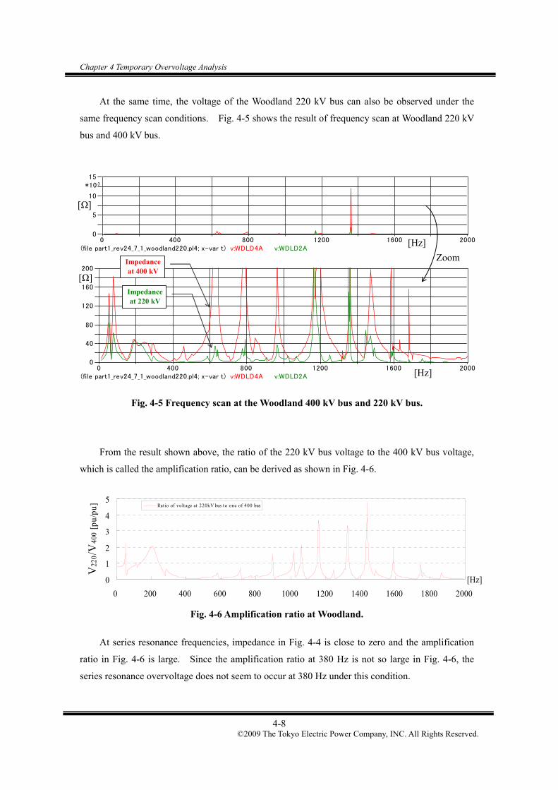
Chapter 4 Temporary Overvoltage Analysis
4-8 ©2009 The Tokyo Electric Power Company, INC. All Rights Reserved.
At the same time, the voltage of the Woodland 220 kV bus can also be observed under the
same frequency scan conditions. Fig. 4-5 shows the result of frequency scan at Woodland 220 kV
bus and 400 kV bus.
(file part1_rev24_7_1_woodland220.pl4; x-var t) v:WDLD4A v:WDLD2A 0 400 800 1200 1600 2000
0
5
10
15*103
(file part1_rev24_7_1_woodland220.pl4; x-var t) v:WDLD4A v:WDLD2A 0 400 800 1200 1600 2000
0
40
80
120
160
200
Fig. 4-5 Frequency scan at the Woodland 400 kV bus and 220 kV bus.
From the result shown above, the ratio of the 220 kV bus voltage to the 400 kV bus voltage,
which is called the amplification ratio, can be derived as shown in Fig. 4-6.
Fig. 4-6 Amplification ratio at Woodland.
At series resonance frequencies, impedance in Fig. 4-4 is close to zero and the amplification
ratio in Fig. 4-6 is large. Since the amplification ratio at 380 Hz is not so large in Fig. 4-6, the
series resonance overvoltage does not seem to occur at 380 Hz under this condition.
Zoom
0
1
2
3
4
5
0 200 400 600 800 1000 1200 1400 1600 1800 2000
[Hz]
V22
0/V
400
[pu
/pu] Rat io of voltage at 220kV bus to one of 400 bus
[Hz]
[Hz]
[Ω]
[Ω] Impedance at 220 kV
Impedance at 400 kV

Chapter 4 Temporary Overvoltage Analysis
4-9 ©2009 The Tokyo Electric Power Company, INC. All Rights Reserved.
[Time domain simulation for the normal condition]
Time domain simulation was conducted for the normal operating condition. Fig. 4-7 and Fig.
4-8 show voltage waveforms when the Woodland – Kingscourt line is energised from the Woodland
side as shown in Fig. 4-3. It did not cause high overvoltage due to series resonance, because the
amplification ratio of the 220 kV bus voltage to the 400 kV bus voltage is very small as shown in
Fig. 4-6.
(Phase to earth)
(file Part1_rev24_7_1_Woodland220_time.pl4; x-var t) v:WDLD4A v:WDLD2A 0.00 0.02 0.04 0.06 0.08 0.10 0.12 0.14 0.16
-400
-300
-200
-100
0
100
200
300
400*10 3
Fig. 4-7 Waveforms of the switching overvoltage at Woodland 400 kV and 220 kV buses
(phase to earth).
(Phase to Phase)
(file Part1_rev24_7_1_Woodland220_time.pl4; x-var t) v:WDLD2A-v:WDLD2B v:WDLD2B-v:WDLD2C v:WDLD2C-v:WDLD2A 0 10 20 30 40 50 60 70 80[ms]
-400
-300
-200
-100
0
100
200
300
400[kV]
Fig. 4-8 Waveforms of the switching overvoltage at the Woodland 220 kV bus (phase to
phase).
Voltage at 400 kV bus 359kV
Voltage at 220 kV bus 193kV
Phase C –Phase A: 320 kV

Chapter 4 Temporary Overvoltage Analysis
4-10 ©2009 The Tokyo Electric Power Company, INC. All Rights Reserved.
Fig. 4-9 and Fig. 4-10 respectively show frequency component spectrums derived from the
voltage waveforms at Woodland 400 kV and 220 kV buses. The frequency components in the
figures were calculated for one cycle immediately after line energisation. Comparing Fig. 4-9 to
Fig. 4-10, the amplification ratio around 200Hz is relatively large, but in a higher frequency range,
the amplification ratio is small.
MC's P lotXY - Four ie r chart(s) . Copying date : 2009/02/27File Part1_rev24_7_1_Woodland220_time.pl4 Variable v:WDLD4A [|pu of harm. 1|]Initial Time: 1.200E-03 Final Time: 0.0212
0 5 10 15 20 25 30 35 400.0
0.2
0.4
0.6
0.8
1.0
harmonic order
Fig. 4-9 Frequency component spectrum of the voltage waveform at the Woodland 400 kV
bus.
MC's P lotXY - Four ie r chart(s) . Copying date : 2009/02/27File Part1_rev24_7_1_Woodland220_time.pl4 Variable v:WDLD2A [|pu of harm. 1|]Initial Time: 1.200E-03 Final Time: 0.0212
0 5 10 15 20 25 30 35 400.0
0.2
0.4
0.6
0.8
1.0
harmonic order
Fig. 4-10 Frequency component spectrum of the voltage waveform at the Woodland 220 kV
bus.

Chapter 4 Temporary Overvoltage Analysis
4-11 ©2009 The Tokyo Electric Power Company, INC. All Rights Reserved.
(2) Assumed most severe condition:
(2) –1 Series resonance frequency 200 Hz
[Frequency scan]
From Fig. 4-5 and Fig. 4-6, it can be seen that the Woodland 220 kV system is under the series
resonance condition at around 200 Hz. The assumed most severe condition can be caused when
the overvoltage caused by the energisation of the 400 kV Woodland – Kingscourt line contains a
large 200 Hz component.
The overvoltage caused by the line energisation generally contains frequency components that
are determined by parallel resonance frequencies and propagation time (τ) in addition to 50 Hz. It
is possible to adjust 1/4τ to series resonance frequency, but it is not possible to match one of
parallel resonance frequencies to series resonance frequency. Hence, in order to generate a 200
Hz component by line energisation, it is necessary to adjust the length of the 400 kV Woodland –
Kingscourt line to satisfy the equation 1/4τ = 200 Hz.
In order to satisfy the equation, the total length of the 400 kV Dunstown – Maynooth –
Woodland – Kingscourt cable line must be equal to
m 212500Hz 200
m/s107.1
4
1 8
The system configuration for the calculation is shown in Fig. 4-11. Target frequency of the
cable models was set to 200 Hz.
WDLD4LCC
125. km
MNPT4 OLDS4LCC
105. km
WMDL4
LCC
85. km
LAOI4LCC
85.23 km
DNST4LCC
44.77 km
Load
60km
KELL4
GR
OU
Pke
l-la
o
WDLD2Y Y
I-Phi
Y Y
I-Phi
OLDS2
standard
YY
WMDL2
standard
YYLAOI2
standard
YY
59.3km
0.0L 0.0
V
MNYPGSAT
Y Y
TRBT1SAT
Y Y
SAT
Y Y
standard
YY
standard
YY
50MVA
50MVATRBT4
KELL2
standard
YY
53.154km
GR
OU
Pw
dl-k
in
DNST2
standard
YYTRBT2
standard
YY
50MVA
50MVA
0.0L 0.0
V
61km 80MVA x 1
18.43kmCORD2
17.83km
0.0L 0.0
V
0.0L 0.0V
0.0L 0.0V
0.0L 0.0V
0.0L 0.0V
4.5kmX0450
30.55km
MAYN4GROUPdun-may
3.73
Load
Load
Load
22.5km
GR
OU
Pw
dl-m
ay
53.154km
GR
OU
Pw
dl-k
in
0.0L 0.0V
0.0L 0.0V
0.0L 0.0V
GROUPreactor
1.4km
MAYN4 MAYN2
standard
YY
6.5km
GROUPmp-tb
GROUPmp-tb
X0420
80MVA x 1
Load
Load
0.0L 0.0
V
Load
Load
1A
53.154km
GR
OU
Pw
dl-k
in
80MVar
Fig. 4-11 System configuration for frequency scan.
To Louth S/S

Chapter 4 Temporary Overvoltage Analysis
4-12 ©2009 The Tokyo Electric Power Company, INC. All Rights Reserved.
Fig. 4-12 shows the result of frequency scan at the Woodland 220 kV and 400 kV bus.
(file Part1_rev24_7_1_Woodland220_159.pl4; x-var t) v:WDLD4A v:WDLD2A 0 400 800 1200 1600 2000
0
50
100
150
200
250
300
Fig. 4-12 Frequency scan at Woodland 400 kV bus and 220 kV.
[Time domain simulation]
Fig. 4-13 and Fig. 4-14 show the waveform of the overvoltage when the 400 kV Woodland –
Kingscourt line is energised from the Woodland side as shown in Fig. 4-3. It did not cause severe
series resonance overvoltage.
(Phase to earth)
(file Part1_rev24_7_1_Woodland220_159_time.pl4; x-var t) v:WDLD2A v:WMDL4A 0.00 0.02 0.04 0.06 0.08 0.10 0.12 0.14 0.16
-400
-300
-200
-100
0
100
200
300
400*10 3
Fig. 4-13 Waveform of the overvoltage at the Woodland 400 kV and 220 kV buses.
Voltage at 220 kV bus 183kV
Voltage at 400 kV bus 366kV
Target frequency: 200Hz Impedance at 220 kV
Impedance at 400 kV
[Ω]
[Hz]

Chapter 4 Temporary Overvoltage Analysis
4-13 ©2009 The Tokyo Electric Power Company, INC. All Rights Reserved.
(Phase to phase)
(file Part1_rev24_7_1_Woodland220_159_time.pl4; x-var t) v:WDLD2A-v:WDLD2B v:WDLD2B-v:WDLD2C v:WDLD2C-v:WDLD2A 0 10 20 30 40 50 60 70 80[ms]
-350.0
-262.5
-175.0
-87.5
0.0
87.5
175.0
262.5
350.0[kV]
Fig. 4-14 Waveforms of the switching overvoltage at the Woodland 220 kV bus (phase to
phase).
Fig. 4-15 and Fig. 4-16 respectively show frequency component spectrums derived from the
voltage waveforms at the Woodland 400 kV and 220 kV buses.
MC's P lotXY - Four ie r chart(s) . Copying date : 2009/02/27File Part1_rev24_7_1_Woodland220_159_time.pl4 Variable v:WDLD4A [|pu of harm. 1|]Initial Time: 1.200E-03 Final Time: 0.0212
0 5 10 15 20 25 30 35 400.0
0.2
0.4
0.6
0.8
1.0
harmonic order
Fig. 4-15 Frequency component spectrum of the switching waveform at the Woodland 400 kV
bus.
MC's P lotXY - Four ie r chart(s) . Copying date : 2009/02/27File Part1_rev24_7_1_Woodland220_159_time.pl4 Variable v:WDLD2A [|pu of harm. 1|]Initial Time: 1.200E-03 Final Time: 0.0212
0 5 10 15 20 25 30 35 400.0
0.2
0.4
0.6
0.8
1.0
harmonic order
Fig. 4-16 Frequency component spectrum of the switching waveform at the Woodland 220 kV
bus.
Phase A –Phase B: 299 kV

Chapter 4 Temporary Overvoltage Analysis
4-14 ©2009 The Tokyo Electric Power Company, INC. All Rights Reserved.
Comparing Fig. 4-15 to Fig. 4-16, it can be found that the 200 Hz component is slightly
amplified from the Woodland 400 kV bus to the Woodland 220 kV bus. However, the magnitude
of 200 Hz component is very small in both the Woodland 400 kV and 220 kV buses. It is
expected that the frequency components contained in the energisation overvoltage were highly
damped due to the long length of the 400 kV Dunstown – Maynooth – Woodland – Kingscourt line.

Chapter 4 Temporary Overvoltage Analysis
4-15 ©2009 The Tokyo Electric Power Company, INC. All Rights Reserved.
(2) –2 Series resonance frequency 1430 Hz
[Frequency scan]
In Fig. 4-6, the largest amplification ratio was found at around 1430 Hz. Here, the total
length of the 400 kV Woodland – Kingscourt line was adjusted to satisfy the equation 1/4τ = 1430
Hz. The calculated total length is
m 29700Hz 4301
m/s107.1
4
1 8
Compensation rate of the cable was set to be approximately equal to the original length as
shown in Table 4-1.
Table 4-1 Compensation of Compensation Rates
The system configuration for frequency scan is shown in Fig. 4-17. The 400 kV Woodland –
Maynooth line is assumed to be out of service to satisfy 1/4τ = 1430 Hz.
Fig. 4-17 System configuration for a frequency scan.
WDLD4LCC
125. km
MNPT4 OLDS4LCC
105. km
WMDL4
LCC
85. km
LAOI4LCC
85.23 km
DNST4LCC
44.77 km
Load
60km
KELL4
GR
OU
Pke
l-la
o
WDLD2Y Y
I-Phi
Y Y
I-Phi
OLDS2
standard
YY
WMDL2
standard
YYLAOI2
standard
YY
59.3km
0.0L 0.0
V
MNYPGSAT
Y Y
TRBT1SAT
Y Y
SAT
Y Y
standard
YY
standard
YY
50MVA
50MVATRBT4
KELL2
standard
YY
29.7km
WDLD4
GR
OU
Pw
dl-k
in
DNST2
standard
YYTRBT2
standard
YY
50MVA
50MVA
0.0L 0.0
V
61km 80MVA x 1
18.43kmCORD2
17.83km
0.0L 0.0
V
0.0L 0.0V
0.0L 0.0V
0.0L 0.0V
0.0L 0.0V
4.5kmX0450
30.55km
MAYN4GROUPdun-may
3.73km
Load
Load
Load
GR
OU
Pw
dl-m
ay
GR
OU
Pw
dl-k
in
GROUPreactor
1.4km
MAYN4 MAYN2
standard
YY
6.5km
GROUPmp-tb
GROUPmp-tb
X0420
80MVA x 1
Load
Load
0.0L 0.0
V
Load
Load
1A
80MVar
Length 58 km (Original) 29.7 kmCharging capacity 539.2 MVA/cct 276.1 MVA/cct
Woodland Kingscourt Woodland KingscourtReactor 300 MVA 240 MVA 150 MVA 120 MVA
(150 * 2) (120 * 2) (150 * 1) (120 * 1)Total 540 MVA Total 270 MVA
Compensation rate 100.1% 97.8%
To Louth S/S
Outage

Chapter 4 Temporary Overvoltage Analysis
4-16 ©2009 The Tokyo Electric Power Company, INC. All Rights Reserved.
Fig. 4-18 shows the result of frequency scan at the Woodland 220 kV and 400 kV bus. It
appears that the series resonance condition is not severe at 1430 Hz.
(file Part1_rev24_7_1_Woodland220_30km.pl4; x-var t) v:WDLD4A v:WDLD2A 0 400 800 1200 1600 2000
0
500
1000
1500
2000
(file Part1_rev24_7_1_Woodland220_30km.pl4; x-var t) v:WDLD4A v:WDLD2A 1400 1420 1440 1460 1480 15000
50100150200250300350400
Fig. 4-18 Frequency scan at the Woodland 400 kV and 220 kV bus.
Fig. 4-19 shows the comparison of 400 kV Woodland bus voltages with the original and its
modified line length. The figure illustrates why the series resonance condition at 1430 Hz is not
very severe in Fig. 4-18. As can be seen from the figure, the frequency response has changed due
to an outage of the 400 kV Woodland – Maynooth line and the change of the 400 kV Woodland –
Kingscourt line length.
Part1_rev24_7_1_Woodland220_30km.pl4: v:WDLD4A part1_rev24_7_1_woodland220.pl4: v:WDLD4A
0 400 800 1200 1600 20000
40
80
120
160
200
Fig. 4-19 Comparison of different conditions with respect to 400 kV cable length.
Target frequency: 1430HzZoom
Impedance at 400 kV bus, Length of 400 kV Woodland – Kingscourt cable: 58km
Impedance at 400 kV bus, Length of 400 kV Woodland – Kingscourt cable: 29.7km
1430Hz
[Hz]
[Ω]
[Ω]
[Hz]
Impedance at 220 kV
Impedance at 400 kV
[Ω]
[Hz]

Chapter 4 Temporary Overvoltage Analysis
4-17 ©2009 The Tokyo Electric Power Company, INC. All Rights Reserved.
(3) Simplified system
The study in (2) Assumed most severe condition shows the difficulty of matching series
resonance frequency to the dominant frequency in the overvoltage intentionally. In order to search
for the most severe condition, parametric studies were performed in (4) and (5). For the
parametric studies, the system has to be simplified so that the effect of the changes can be
theoretically understood. For this objective, the following changes were introduced to the normal
conditions:
It was assumed that all the Woodland 220 kV system was fed from other substations except
the 220 kV Woodland – Louth line.
The Woodland 220 kV system was separated from the Louth 220 kV system.
The 400 kV Woodland – Maynooth line was out of service.
The loads at Corduff and Finglas were removed together from the simulation model due to this
simplification, which will lead to a severe condition.
WDLD4LCC
125. km
MNPT4 OLDS4LCC
105. km
WMDL4
LCC
85. km
LAOI4LCC
85.23 km
DNST4LCC
44.77 km
220.2L-12.4X0188
V
Load
60km
KELL4
GR
OU
Pke
l-la
o
WDLD2Y Y
I-Phi
Y Y
I-Phi
OLDS2
standard
YY
WMDL2
standard
YYLAOI2
standard
YY
59.3km
0.0L 0.0
VMNYPGSAT
Y Y
TRBT1SAT
Y Y
SAT
Y Y
standard
YY
standard
YY
50MVA
50MVATRBT4
KELL2
standard
YY
DNST2
standard
YYTRBT2
standard
YY
220.L-12.4
V
61km 80MVA x 1
403.5L-12.4
V
413.6L-12.4V
426.9L-16.4V
436.4L-20.1V
446.8L-21.5V
30.55km
MAYN4GROUPdun-may
Load
Load
Load
GR
OU
Pw
dl-m
ay
17kV
110kV
GR
OU
Pw
dl-k
in
GROUPreactor
MAYN4 MAYN2
standard
YY
6.5km
GROUPmp-tb
GROUPmp-tb
80MVA x 1
447.1L-21.9
V
Load
Load
284.2L-12.4
V
399.6L-12.4
V
58km
GR
OU
Pw
dl-k
in
80MVar
Fig. 4-20 Simplified system configuration for parametric studies.
Removed
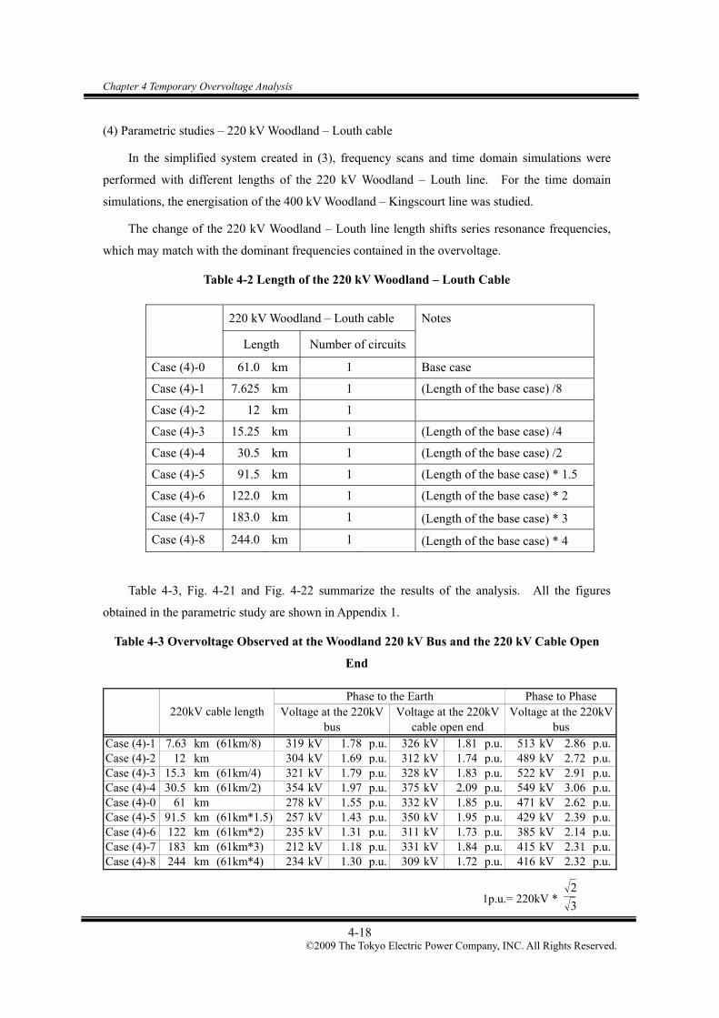
Chapter 4 Temporary Overvoltage Analysis
4-18 ©2009 The Tokyo Electric Power Company, INC. All Rights Reserved.
(4) Parametric studies – 220 kV Woodland – Louth cable
In the simplified system created in (3), frequency scans and time domain simulations were
performed with different lengths of the 220 kV Woodland – Louth line. For the time domain
simulations, the energisation of the 400 kV Woodland – Kingscourt line was studied.
The change of the 220 kV Woodland – Louth line length shifts series resonance frequencies,
which may match with the dominant frequencies contained in the overvoltage.
Table 4-2 Length of the 220 kV Woodland – Louth Cable
220 kV Woodland – Louth cable
Length Number of circuits
Notes
Case (4)-0 61.0 km 1 Base case
Case (4)-1 7.625 km 1 (Length of the base case) /8
Case (4)-2 12 km 1
Case (4)-3 15.25 km 1 (Length of the base case) /4
Case (4)-4 30.5 km 1 (Length of the base case) /2
Case (4)-5 91.5 km 1 (Length of the base case) * 1.5
Case (4)-6 122.0 km 1 (Length of the base case) * 2
Case (4)-7 183.0 km 1 (Length of the base case) * 3
Case (4)-8 244.0 km 1 (Length of the base case) * 4
Table 4-3, Fig. 4-21 and Fig. 4-22 summarize the results of the analysis. All the figures
obtained in the parametric study are shown in Appendix 1.
Table 4-3 Overvoltage Observed at the Woodland 220 kV Bus and the 220 kV Cable Open
End
Case (4)-1 7.63 km (61km/8) 319 kV 1.78 p.u. 326 kV 1.81 p.u. 513 kV 2.86 p.u.Case (4)-2 12 km 304 kV 1.69 p.u. 312 kV 1.74 p.u. 489 kV 2.72 p.u.Case (4)-3 15.3 km (61km/4) 321 kV 1.79 p.u. 328 kV 1.83 p.u. 522 kV 2.91 p.u.Case (4)-4 30.5 km (61km/2) 354 kV 1.97 p.u. 375 kV 2.09 p.u. 549 kV 3.06 p.u.Case (4)-0 61 km 278 kV 1.55 p.u. 332 kV 1.85 p.u. 471 kV 2.62 p.u.Case (4)-5 91.5 km (61km*1.5) 257 kV 1.43 p.u. 350 kV 1.95 p.u. 429 kV 2.39 p.u.Case (4)-6 122 km (61km*2) 235 kV 1.31 p.u. 311 kV 1.73 p.u. 385 kV 2.14 p.u.Case (4)-7 183 km (61km*3) 212 kV 1.18 p.u. 331 kV 1.84 p.u. 415 kV 2.31 p.u.Case (4)-8 244 km (61km*4) 234 kV 1.30 p.u. 309 kV 1.72 p.u. 416 kV 2.32 p.u.
Phase to PhaseVoltage at the 220kV
busVoltage at the 220kV
cable open endVoltage at the 220kV
bus
Phase to the Earth220kV cable length
1p.u.= 220kV *3
2

Chapter 4 Temporary Overvoltage Analysis
4-19 ©2009 The Tokyo Electric Power Company, INC. All Rights Reserved.
(Phase to earth)
Fig. 4-21 Overvoltage observed at the Woodland 400 kV and 220 kV buses and 220 kV cable
open end (phase to earth).
(Phase to phase)
489
549
471429
385415 416
513 522
0
100
200
300
400
500
600
0 50 100 150 200 250
Length of 220kV cable [km]
Vol
tage
[kV
peak
]
Voltage at 220kV bus (Phase to Phase)
Fig. 4-22 Overvoltage observed at the Woodland 220 kV bus (phase to phase).
467 451
384
431388
416
304
354
278257
235212
234
312332
476458490
321319
328326375
350
331 309311
0
100
200
300
400
500
600
0 50 100 150 200 250
Length of 220kV cable [km]
Vol
tage
[kV
peak
]
Voltage at 400kV busVoltage at 220kV busVoltage at 220kV cable open end

Chapter 4 Temporary Overvoltage Analysis
4-20 ©2009 The Tokyo Electric Power Company, INC. All Rights Reserved.
(5) Parametric studies – 400 kV Woodland – Kingscourt cable
In the simplified system created in (3), frequency scans and time domain simulations were
performed with different lengths of the 400 kV Woodland – Kingscourt line. For the time domain
simulations, the energisation of the 400 kV Woodland – Kingscourt line was studied.
The change of the 220 kV Woodland – Kingscourt line length shifts dominant frequencies
contained in the energisation overvoltage, which may match with series resonance frequencies.
The compensation rates of the 400 kV cable were kept around 100 % with different lengths of the
cable as shown in Table 4-4.
Table 4-4 Length of the 400 kV Woodland – Kingscourt Line
Table 4-5, Fig. 4-23 and Fig. 4-24 summarize the result of the analysis. All the figures
obtained in the parametric study are shown in Appendix 2.
Table 4-5 Overvoltage Observed at the Woodland 220 kV Bus and the 220 kV Cable Open End
(5)-1 141.7 km 300 Hz 225 kV 1.25 p.u. 243 kV 1.35 p.u. 362 kV 2.02 p.u.(5)-2 106.3 km 400 Hz 258 kV 1.44 p.u. 279 kV 1.55 p.u. 421 kV 2.34 p.u.(5)-3 85.0 km 500 Hz 260 kV 1.45 p.u. 326 kV 1.81 p.u. 443 kV 2.47 p.u.(5)-4 70.8 km 600 Hz 278 kV 1.55 p.u. 285 kV 1.59 p.u. 502 kV 2.79 p.u.(5)-5 60.7 km 700 Hz 264 kV 1.47 p.u. 322 kV 1.79 p.u. 478 kV 2.66 p.u.(5)-6 47.2 km 900 Hz 263 kV 1.46 p.u. 305 kV 1.70 p.u. 469 kV 2.61 p.u.(5)-7 38.6 km 1100 Hz 277 kV 1.54 p.u. 318 kV 1.77 p.u. 465 kV 2.59 p.u.(5)-8 26.6 km 1600 Hz 267 kV 1.49 p.u. 344 kV 1.92 p.u. 443 kV 2.47 p.u.(5)-9 22.4 km 1900 Hz 279 kV 1.55 p.u. 341 kV 1.90 p.u. 441 kV 2.46 p.u.
Phase to the Earth Phase to PhaseVoltage at the 220kV
bus
1p.u.= 220kV *
400kVcablelength
Targetfrequency
Voltage at the 220kVbus
Voltage at the 220kVcable open end
3
2
Woodland Kingscourt(5)- 1 141.7 km 300 Hz 1,317 MVA 750 MVA 600 MVA 102.5%(5)- 2 106.3 km 400 Hz 988 MVA 600 MVA 360 MVA 97.2%(5)- 3 85.0 km 500 Hz 790 MVA 450 MVA 360 MVA 102.5%(5)- 4 70.8 km 600 Hz 659 MVA 300 MVA 360 MVA 100.2%(5)- 5 60.7 km 700 Hz 564 MVA 300 MVA 300 MVA 106.3%(5)- 6 47.2 km 900 Hz 439 MVA 300 MVA 120 MVA 95.7%(5)- 7 38.6 km 1100 Hz 359 MVA 240 MVA 120 MVA 100.2%(5)- 8 26.6 km 1600 Hz 247 MVA 120 MVA 120 MVA 97.2%(5)- 9 22.4 km 1900 Hz 208 MVA 120 MVA 120 MVA 115.4%
9.3 MVA/cct/km
400kVcable
Targetfrequency
Chargingcapacity
Charging capacity:
Compensationrate
Reactor for 400kV cable

Chapter 4 Temporary Overvoltage Analysis
4-21 ©2009 The Tokyo Electric Power Company, INC. All Rights Reserved.
(Phase to earth)
Fig. 4-23 Overvoltage observed at the Woodland 400 kV and 220 kV buses and 220 kV cable
open end (phase to earth).
(Phase to phase)
421
502478469465
441 443
362
443
0
100
200
300
400
500
600
0.0 20.0 40.0 60.0 80.0 100.0 120.0 140.0
Length of 400kV cable [km]
Vol
tage
[kV
peak
]
Voltage at 220kV bus (Phase to Phase)
Fig. 4-24 Overvoltage observed at the Woodland 220 kV bus (phase to phase).
430444466
498472
258285
264263277279
279322
491
338383 378
267
225
260
318341 344305
278243
326
0
100
200
300
400
500
600
0.0 20.0 40.0 60.0 80.0 100.0 120.0 140.0
Length of 400kV cable [km]
Vol
tage
[kV
peak
]
Voltage at 400kV busVoltage at 220kV busVoltage at 220kV cable open end

Chapter 4 Temporary Overvoltage Analysis
4-22 ©2009 The Tokyo Electric Power Company, INC. All Rights Reserved.
4.1.2 Resonance overvoltage in the Turleenan 275 kV system
Fig. 4-25 shows the system configuration for the series resonance overvoltage analysis in the
Turleenan 275 kV system caused by the energisation of the 400 kV Kingscourt – Turleenan line
from the Turleenan S/S.
WoodlandTurleenan
(Observing point) KingscourtMNYPG
CoolkeeraghOmagh
Flagford
Turleenan275kV
Close
Open
Fig. 4-25 System configuration for series resonance overvoltage in Turleenan 275 kV system.
Fig. 4-26 shows a result of frequency scan. The vertical axis of the figure shows voltages
observed at the Turleenan 400 kV, which is equal to the equivalent impedance of the network seen
from the Turleenan 400 kV bus because the injected current is 1 Amp.

Chapter 4 Temporary Overvoltage Analysis
4-23 ©2009 The Tokyo Electric Power Company, INC. All Rights Reserved.
(file part1_rev24_7_4_turleenan275.pl4; x-var t) v:TURL4A 0 400 800 1200 1600 2000
01000200030004000500060007000
(file part1_rev24_7_4_turleenan275.pl4; x-var t) v:TURL4A 0 400 800 1200 1600 2000
0
40
80
120
160
200
Fig. 4-26 Frequency scan at Turleenan 400 kV bus in the normal condition.
Fig. 4-27 shows the result of frequency scan at the Turleenan 400 kV and 275 kV buses, and
the amplification ratio from Turleenan 400 kV to 275 kV bus voltage is shown in Fig. 4-28.
(file part1_rev24_7_4_turleenan275.pl4; x-var t) v:TURL4A v:TURL2A 0 400 800 1200 1600 2000
0100020003000
4000500060007000
(file part1_rev24_7_4_turleenan275.pl4; x-var t) v:TURL4A v:TURL2A 0 400 800 1200 1600 2000
0
40
80
120
160
200
Fig. 4-27 Frequency scan at Turleenan 400 kV and 275 kV bus in the normal condition.
115Hz 127Hz
Zoom 781Hz
277Hz
Zoom
[Ω]
[Hz]
[Ω]
[Hz]
[Ω]
[Hz]
[Ω]
[Hz]

Chapter 4 Temporary Overvoltage Analysis
4-24 ©2009 The Tokyo Electric Power Company, INC. All Rights Reserved.
Fig. 4-28 Amplification ratio at Turleenan.
Series resonance frequencies were found at 115 Hz, 128 Hz, 351 Hz, and 534 Hz.
[Time domain simulations in the normal condition]
The energisation of the 400 kV Kingscourt – Turleenan line was studied under normal
conditions. Fig. 4-29 and Fig. 4-30 show the overvoltage in the Turleenan 400 kV and 275 kV
buses. It was found that the energisation of the 400 kV Kingscourt – Turleenan line did not cause
high overvoltage due to series resonance.
(Phase to earth)
(file Part1_rev24_7_4_Turleenan275_time.pl4; x-var t) v:X0139A v:TURL2A 0 10 20 30 40 50 60 70 80[ms]
-400
-300
-200
-100
0
100
200
300
400[kV]
Fig. 4-29 Waveforms of the overvoltage at Turleenan 400 kV and 275 kV buses (phase to
earth).
0123456789
10
0 200 400 600 800 1000 1200 1400 1600 1800 2000
[Hz]
V27
5/V
400
[pu
/pu] Rat io of voltage at 275kV bus to one of 400 bus
115Hz, 128Hz
351Hz
534Hz
Voltage at 400 kV bus 396kV
Voltage at 275 kV bus 228kV

Chapter 4 Temporary Overvoltage Analysis
4-25 ©2009 The Tokyo Electric Power Company, INC. All Rights Reserved.
(Phase to phase)
(file Part1_rev24_7_4_Turleenan275_time.pl4; x-var t) v:TURL2A-v:TURL2B v:TURL2B-v:TURL2C v:TURL2C-v:TURL2A 0 10 20 30 40 50 60 70 80[ms]
-400
-300
-200
-100
0
100
200
300
400[kV]
Fig. 4-30 Waveforms of the overvoltage at the Turleenan 275 kV bus (phase to phase).
Phase A –Phase B: 392 kV

Chapter 4 Temporary Overvoltage Analysis
4-26 ©2009 The Tokyo Electric Power Company, INC. All Rights Reserved.
The Fourier transforms of the waveforms for 100 ms yield frequency components by 10 Hz
step. Fig. 4-31 and Fig. 4-32 respectively show frequency components contained in the voltage
waveform at the Turleenan 400 kV and 275 kV buses.
Fig. 4-31 Frequency components in the waveform at the Turleenan 400 kV bus.
0
10
20
30
40
0 200 400 600 800 1000 1200 1400 1600 1800 2000 [Hz]
Am
plit
ude
[kV
]
Voltage at T urleenan 400kV bus
Zoom
32kV at 180Hz
Zoom
0
100
200
300
400
0 200 400 600 800 1000 1200 1400 1600 1800 2000 [Hz]
Am
plitu
de [
kV] Voltage at T urleenan 400kV bus
0.6 0.62.0
3.7
6.6
313.5
8.5
13.711.3
7.7
3.91.7 0.7 0.6
2.7
5.8
11.7
28.4
31.9
15.5
10.9
0
10
20
30
40
0 20 40 60 80 100 120 140 160 180 200 [Hz]
Am
plitu
de [
kV]
Voltage at T urleenan 400kV bus

Chapter 4 Temporary Overvoltage Analysis
4-27 ©2009 The Tokyo Electric Power Company, INC. All Rights Reserved.
Fig. 4-32 Frequency components in the waveform at the Turleenan 275 kV bus.
0
2
4
6
8
10
0 200 400 600 800 1000 1200 1400 1600 1800 2000 [Hz]
Am
plit
ude
[kV
]
Voltage at T urleenan 275kV bus
Zoom
050
100
150200250
0 200 400 600 800 1000 1200 1400 1600 1800 2000 [Hz]
Am
plitu
de [
kV]
Voltage at T urleenan 275kV bus
Zoom
-0.10.5
1.12.0
3.8
215.2
6.6
8.1 8.3
6.4
4.43.4
2.8 3.2 3.1 3.44.4
7.2
5.6
1.9
0.8
0
2
4
6
8
10
12
14
0 20 40 60 80 100 120 140 160 180 200 [Hz]
Am
plit
ude
[kV
]
Volt age at T urleenan 275kV bus
8kV at 80Hz
7kV at 170Hz

Chapter 4 Temporary Overvoltage Analysis
4-28 ©2009 The Tokyo Electric Power Company, INC. All Rights Reserved.
The amplification ratio from the Turleenan 400 kV bus to the 275 kV bus can be derived from
Fig. 4-31 and Fig. 4-32. The obtained amplification ratio is shown in Fig. 4-33.
Fig. 4-33 Amplification ratio of voltage from the Turleenan 400 kV bus to the 275 kV bus.
Results from the frequency scan showed that series resonance frequencies were found at 115
Hz, 128 Hz, 351 Hz, and 534 Hz as shown in Fig. 4-28. Results from the time domain simulation
showed that series resonance frequencies were found at 130 Hz, 350 Hz, and 530 Hz as depicted in
Fig. 4-33. It is apparent that series resonance frequencies found by two different approaches
closely match with each other.
As a result, the parametric study of the Turleenan 275 kV system could not find a severe series
resonance condition. Instead, the study came across a parallel resonance condition, which is not
described in this public report, at 50 Hz, and it should be avoided while operating the network.
Fortunately, the condition assumed for parallel resonance was extreme which may be realized only
during a black-start operation. The result shows the necessity of studying parallel resonance when
establishing a black-start procedure in the NIE network.
01234567
0 200 400 600 800 1000 1200 1400 1600 1800 2000[Hz]
Vol
tage
rat
io [
pu/p
u] Rat io of Voltage at 275kV bus toVoltage at 400kV bus
130Hz
350Hz
530Hz

Chapter 4 Temporary Overvoltage Analysis
4-29 ©2009 The Tokyo Electric Power Company, INC. All Rights Reserved.
4.1.3 Resonance overvoltage in the Kingscourt 220 kV system by the
energisation of the Kingscourt – Turleenan line
Fig. 4-34 shows the system configuration for the series resonance overvoltage analysis in the
Kingscourt 220 kV system caused by the energisation of the 400 kV Kingscourt – Turleenan line
from the Kingscourt S/S.
Fig. 4-34 System configuration for the series resonance overvoltage analysis in Kingscourt 220
kV system.
Target frequency of the 400 kV cable is calculated considering the total cable length from
Dunstown to Turleenan.
Hz220m)000,82000,58500,22550,30(
m/s107.1
4
1f
8

Chapter 4 Temporary Overvoltage Analysis
4-30 ©2009 The Tokyo Electric Power Company, INC. All Rights Reserved.
Fig. 4-35 shows the result of frequency scan under normal conditions. The vertical axis of
the figure shows the voltages observed at the Kingscourt 400 kV bus, which is equal to the
magnitude of impedance of the network seen from the Kingscourt 400 kV bus.
(file part1_rev24_7_2_kingscourt220_tside.pl4; x-var t) v:KING4A 0 400 800 1200 1600 2000
0
100
200
300
400
500
Fig. 4-35 Frequency scan at Kingscourt in the normal condition.
Fig. 4-36 shows the result of frequency scan at the Kingscourt 220 kV and 400 kV buses, and
Fig. 4-37 shows the amplification ratio from the Kingscourt 400 kV bus to the 220 kV bus.
Fig. 4-36 Frequency scan at the Kingscourt 400 kV and 220 kV buses in the normal condition.
(file part1_rev24_7_2_kingscourt220_tside.pl4; x-var t) v:KING4A v:KING2A 0 400 800 1200 1600 2000
0
100
200
300
400
500
273Hz
[Ω]
[Hz]

Chapter 4 Temporary Overvoltage Analysis
4-31 ©2009 The Tokyo Electric Power Company, INC. All Rights Reserved.
Fig. 4-37 Amplification ratio at Kingscourt.
Series resonance frequency was not found at 1/4τ = 220 Hz.
Fig. 4-38 and Fig. 4-39 show the results of the time domain simulation under normal
conditions.
(Phase to earth)
(file Part1_rev24_7_1_Kingscourt220_Tside_time.pl4; x-var t) v:X0325A v:KING2A 0 10 20 30 40 50 60 70 80[ms]
-400
-300
-200
-100
0
100
200
300
400[kV]
Fig. 4-38 Waveforms of the overvoltage at the Kingscourt 400 kV and 220 kV buses (phase to earth).
(Phase to phase)
(file Part1_rev24_7_1_Kingscourt220_Tside_time.pl4; x-var t) v:KING2A-v:KING2B v:KING2B-v:KING2C v:KING2C-v:KING2A 0 10 20 30 40 50 60 70 80[ms]
-350.0
-262.5
-175.0
-87.5
0.0
87.5
175.0
262.5
350.0[kV]
Fig. 4-39 Waveforms of the overvoltage at the 220 kV buses bus (phase to phase).
0
1
2
3
4
0 200 400 600 800 1000 1200 1400 1600 1800 2000
[Hz]
V22
0/V
400
[pu
/pu] Rat io of voltage at 275kV bus to one of 400 bus63Hz 114Hz
280Hz 457Hz
896Hz
713Hz 1162Hz
1587Hz
Voltage at the 400 kV bus: 339kV
Voltage at the 220 kV bus:176kV
Phase C –Phase A: 302 kV

Chapter 4 Temporary Overvoltage Analysis
4-32 ©2009 The Tokyo Electric Power Company, INC. All Rights Reserved.
Fig. 4-40 and Fig. 4-41 respectively show frequency component spectrums derived from the
voltage waveforms at the Kingscourt 400 kV and 220 kV buses. The frequency components were
calculated for one cycle immediately after the line energisation.
From these figures, it can be seen that harmonic components contained in the energisation
overvoltage are very low. In addition, since 1/4τ does not match series resonance frequencies,
severe resonance overvoltage was not observed in the simulation result.
MC's P lotXY - Four ie r chart(s) . Copying date : 2009/03/03File Part1_rev24_7_1_Kingscourt220_Tside_time.pl4 Variable v:X0325A [|pu of harm. 1|]Initial Time: 0.01102 Final Time: 0.03102
0 5 10 15 20 25 30 35 400.0
0.5
1.0
harmonic order
Fig. 4-40 Frequency component spectrum of the switching waveform at the Kingscourt 400
kV bus
MC's P lotXY - Four ie r chart(s) . Copying date : 2009/03/03File Part1_rev24_7_1_Kingscourt220_Tside_time.pl4 Variable v:KING2A [|pu of harm. 1|]Initial Time: 0.01102 Final Time: 0.03102
0 5 10 15 20 25 30 35 400.0
0.5
1.0
harmonic order
Fig. 4-41 Frequency component spectrum of the switching waveform at the Kingscourt 220
kV bus

Chapter 4 Temporary Overvoltage Analysis
4-33 ©2009 The Tokyo Electric Power Company, INC. All Rights Reserved.
4.1.4 Resonance overvoltage in the Kingscourt 220 kV system by the
energisation of the Woodland – Kingscourt line
Fig. 4-42 shows the system configuration for the series resonance overvoltage analysis in the
Kingscourt 220 kV system caused by the energisation of the 400 kV Woodland – Kingscourt line
from the Kingscourt S/S.
Fig. 4-42 System configuration for the series resonance overvoltage analysis in the Kingscourt
220 kV system.
Target frequency of the 400 kV cable is calculated considering the total cable length from
Woodland to Turleenan.
Hz300m)000,82000,58(
m/s107.1
4
1f
8

Chapter 4 Temporary Overvoltage Analysis
4-34 ©2009 The Tokyo Electric Power Company, INC. All Rights Reserved.
Fig. 4-43 shows the result of frequency scan under normal conditions. The vertical axis of
the figure shows the voltages observed at the Kingscourt 400 kV bus, which is equal to the
magnitude of impedance of the network seen from the Kingscourt 400 kV bus.
(file part1_rev24_7_3_kingscourt220_wside.pl4; x-var t) v:KING4A 0 400 800 1200 1600 2000
0
200
400
600
800
1000
Fig. 4-43 Frequency scan at Kingscourt.
Fig. 4-44 shows the result of frequency scan at the Kingscourt 220 kV and 400 kV buses, and
Fig. 4-45 shows the amplification ratio from the Kingscourt 400 kV bus to the 220 kV bus.
(file part1_rev24_7_3_kingscourt220_wside.pl4; x-var t) v:KING4A v:KING2A 0 400 800 1200 1600 2000
0
200
400
600
800
1000
(file part1_rev24_7_3_kingscourt220_wside.pl4; x-var t) v:KING4A v:KING2A 0 400 800 1200 1600 2000
0
40
80
120
160
200
Fig. 4-44 Frequency scan at the Kingscourt 400 kV and 220 kV buses under normal
conditions.
377Hz 98Hz 818Hz 1866Hz
Zoom
[Ω]
[Hz]
[Ω]
[Hz]
[Ω]
[Hz]

Chapter 4 Temporary Overvoltage Analysis
4-35 ©2009 The Tokyo Electric Power Company, INC. All Rights Reserved.
Fig. 4-45 Amplification ratio at Kingscourt.
Series resonance frequency was not found at 1/4τ = 300 Hz.
Fig. 4-46 and Fig. 4-47 show the result of the time domain simulation under normal conditions.
As in the analysis in Section 3.1.3, harmonic components contained in the energisation overvoltage
are very low. Additionally, since 1/4τ does not match series resonance frequencies, severe
resonance overvoltage was not observed in the simulation result.
(Phase to earth)
(file Part1_rev24_7_1_Kingscourt220_Wside_time.pl4; x-var t) v:KING4A v:KING2A 0 10 20 30 40 50 60 70 80[ms]
-400
-300
-200
-100
0
100
200
300
400[kV]
Fig. 4-46 Waveforms of the overvoltage at the Kingscourt 400 kV and 220kV buses (phase to
earth).
0
1
2
3
4
5
6
7
0 200 400 600 800 1000 1200 1400 1600 1800 2000
[Hz]
V22
0/V
400 [
pu/p
u] Rat io of voltage at 275kV bus to one of 400 bus
89Hz
281Hz
711Hz 897Hz457Hz
1858Hz
Voltage at the 400 kV bus: 316kV
Voltage at the 220 kV bus:171kV

Chapter 4 Temporary Overvoltage Analysis
4-36 ©2009 The Tokyo Electric Power Company, INC. All Rights Reserved.
(Phase to phase)
(file Part1_rev24_7_1_Kingscourt220_Wside_time.pl4; x-var t) v:KING2A-v:KING2B v:KING2B-v:KING2C v:KING2C-v:KING2A 0 10 20 30 40 50 60 70 80[ms]
-300
-200
-100
0
100
200
300
[kV]
Fig. 4-47 Waveforms of the overvoltage at the Kingscourt 220kV bus (phase to phase).
Phase C – Phase A: 292 kV

Chapter 4 Temporary Overvoltage Analysis
4-37 ©2009 The Tokyo Electric Power Company, INC. All Rights Reserved.
4.2 Parallel Resonance Overvoltage
In EHV systems, the highest concern in terms of parallel resonance is the second harmonic
current injection due to transformer inrush. Parallel resonance frequencies will be found from the
results of frequency scan in EMTP.
When the EHV underground cable has significant length, the switching overvoltage caused by
its energisation can have very low frequency components for switching overvoltage. For example,
an energisation of EHV underground cable of a length of around 100 km may largely contain third
to fifth harmonics. Therefore, parallel resonance frequencies higher than 100 Hz (second
harmonic) will also be searched for in frequency scan.
Parallel resonance frequency seen from the Cahir substation for the study of overvoltage caused by transformer inrush current
Parallel resonance frequency seen from the Cahir substation for the study of overvoltage caused by underground cable energisation
Fig. 4-48 Frequency scan for the parallel resonance overvoltage analysis.
Current source (1 Amp)
Outage
Outage
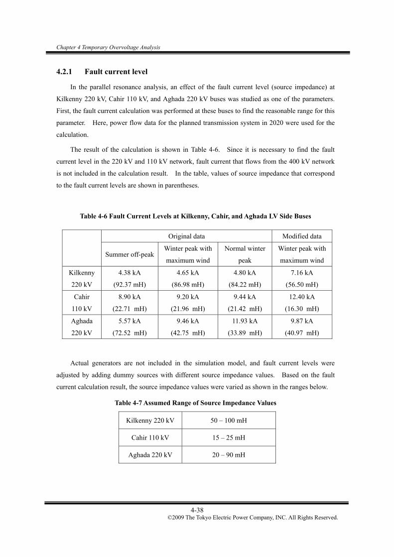
Chapter 4 Temporary Overvoltage Analysis
4-38 ©2009 The Tokyo Electric Power Company, INC. All Rights Reserved.
4.2.1 Fault current level
In the parallel resonance analysis, an effect of the fault current level (source impedance) at
Kilkenny 220 kV, Cahir 110 kV, and Aghada 220 kV buses was studied as one of the parameters.
First, the fault current calculation was performed at these buses to find the reasonable range for this
parameter. Here, power flow data for the planned transmission system in 2020 were used for the
calculation.
The result of the calculation is shown in Table 4-6. Since it is necessary to find the fault
current level in the 220 kV and 110 kV network, fault current that flows from the 400 kV network
is not included in the calculation result. In the table, values of source impedance that correspond
to the fault current levels are shown in parentheses.
Table 4-6 Fault Current Levels at Kilkenny, Cahir, and Aghada LV Side Buses
Original data Modified data
Summer off-peak
Winter peak with
maximum wind
Normal winter
peak
Winter peak with
maximum wind
Kilkenny
220 kV
4.38 kA
(92.37 mH)
4.65 kA
(86.98 mH)
4.80 kA
(84.22 mH)
7.16 kA
(56.50 mH)
Cahir
110 kV
8.90 kA
(22.71 mH)
9.20 kA
(21.96 mH)
9.44 kA
(21.42 mH)
12.40 kA
(16.30 mH)
Aghada
220 kV
5.57 kA
(72.52 mH)
9.46 kA
(42.75 mH)
11.93 kA
(33.89 mH)
9.87 kA
(40.97 mH)
Actual generators are not included in the simulation model, and fault current levels were
adjusted by adding dummy sources with different source impedance values. Based on the fault
current calculation result, the source impedance values were varied as shown in the ranges below.
Table 4-7 Assumed Range of Source Impedance Values
Kilkenny 220 kV 50 – 100 mH
Cahir 110 kV 15 – 25 mH
Aghada 220 kV 20 – 90 mH

Chapter 4 Temporary Overvoltage Analysis
4-39 ©2009 The Tokyo Electric Power Company, INC. All Rights Reserved.
4.2.2 Overvoltage caused by transformer inrush current
Overvoltage caused by transformer inrush current will be studied with the switching scenario
shown in Fig. 4-49.
Kilkenny Cahir Aghada
400kV
400kV
400kV
110kV
220kV220kV
Close
Open
On
Fig. 4-49 Switching scenario for the overvoltage caused by transformer inrush current.
4.2.3 Parallel resonance frequency seen from Cahir 400 kV
Parallel resonance frequency of the network seen from Cahir 400 kV was found by frequency
scan using the simulation model in Fig. 4-50.
112kmX0049 X0068
GROUPagh-chr
X0108
KLKN4
X0108
X0108
AGHD4 KLKN2
V
AGH4T AGH2T
Y Y
I-Phi
VV
X0068
AGHD2
V
X0233
90mH
100mH
CH1T1
Y Y
I-Phi CH1T1
KLK4T KLK2T
Y Y
I-Phi
25mH
60km
GROUPkel-lao
1A
V
V
V
Fig. 4-50 Frequency scan for the parallel resonance overvoltage analysis.
In the first example, the largest source impedance (lowest fault current level) in Table 4-7 was
set to Kilkenny 220 kV, Cahir 110 kV, and Aghada 220 kV buses. The result of this frequency
scan is shown in Fig. 4-51. The highest peak was found at 75 Hz, and the other high peaks were
not the level which required careful consideration.
Current source (1 Amp)
Outage
Cahir – Kilkenny line Aghada – Cahir line
Kilkenny 400/220
kV Trafo Cahir 400/110 kV Trafo Aghada 400/110 kV Trafo.

Chapter 4 Temporary Overvoltage Analysis
4-40 ©2009 The Tokyo Electric Power Company, INC. All Rights Reserved.
(file Fscan_cahir_1bank_outage_Klkn100mH_Chr25mH_Aghd90mH_Peak_50Hz_Aghada-Cahir_length112km(100%)_span3.11km_rev1v:X0108A v:X0108B v:X0108C
0 500 1000 1500 2000 2500 3000[Hz]0
400
800
1200
1600
2000
[ohm]
Fig. 4-51 Parallel resonance frequency of the network seen from Cahir 400 kV.
In deriving parallel resonance frequencies in Fig. 4-51, 220 and 110 kV cable capacitances
were not considered. In order to study the effect of 220 kV cable capacitances, frequency scan
was repeated with different shunt capacitances connected to the Aghada 220 kV bus.
70 72 74 76 78 80[Hz]0
10
20
30
40
50
60
[kΩ]
Fig. 4-52 Effect of shunt capacitance connected to the Aghada 220 kV bus.
As can be seen from Fig. 4-52, parallel resonance frequency goes away from 100 Hz when
220 kV cable capacitances are considered, which makes it difficult to have parallel resonance
75Hz
No capacitance 100 MVar 200 MVar 400 MVar

Chapter 4 Temporary Overvoltage Analysis
4-41 ©2009 The Tokyo Electric Power Company, INC. All Rights Reserved.
frequency at 100 Hz. In addition, equivalent impedance of the network at parallel resonance
frequency does not rise due to the connection of shunt capacitance.
In order to find an effect of the source impedance, the source impedance connected to
Kilkenny 220 kV bus was reduced from 100 mH to 75 mH or 50mH, the source impedance
connected to Cahir 110 kV bus was reduced from 25 mH to 10 mH or 15 mH, the source
impedance connected to Aghada 220 kV bus was reduced from 90 mH to 55 mH or 20 mH.
Table 4-8 Effect of Source Impedance
Kilkenny
220 kV
Cahir
110 kV
Aghada
220 kV
Parallel resonance
frequency [Hz]
Difference
[Hz]
100 mH 75.0 -
75 mH 76.5 +1.5
50 mH
25 mH 90 mH
78.7 +3.7
25 mH 75.0 -
20 mH 75.6 +0.6 100 mH
15 mH
90 mH
76.4 +1.4
90 mH 75.0 -
55 mH 77.8 +2.8 100 mH 25 mH
20 mH 83.0 +8.0
50 mH 15 mH 20 mH 88.0 +13.0
Table 4-8 shows the effect of the source impedance. By changing the source impedance from
the largest values to the smallest values, parallel resonance frequency was shifted by 13.0 Hz.
The result of frequency scan is shown in Fig. 4-53. It can be seen that the magnitude of
impedance at parallel resonance significantly decreases for smaller source impedance (a higher
fault current level).

Chapter 4 Temporary Overvoltage Analysis
4-42 ©2009 The Tokyo Electric Power Company, INC. All Rights Reserved.
fscan_cahir_1bank_outage_klkn100mh_chr25mh_aghd90mh_peak_50hz_aghada-cahir_length112km(100%)_span3.11km_rev1.pl4: v:Xfscan_cahir_1bank_outage_klkn50mh_chr15mh_aghd20mh_peak_50hz_aghada-cahir_length112km(100%)_span3.11km_rev1.pl4: v:X0
60 69 78 87 96 105[Hz]0
10
20
30
40
50
60
[kΩ]
Fig. 4-53 Effect of the source impedance on parallel resonance frequency of the network seen
from Cahir 400 kV.
Then, in order to find the effect of the cable length, the length of the 400 kV Aghada – Cahir
line was varied from 50 % to 200 % by 25 % steps. In this analysis, the compensation rate of
cables was maintained at the same values as that of the original cable length.
Table 4-9 Effect of the Length of 400 kV Aghada-Cahir Cable.
Length
[km]
Span length
[km]
Number of
major cross
bonding sections
Shunt
reactor
[MVA]
Parallel
resonance
frequency
[Hz]
Difference
[Hz]
57 (50%) 3.111 6 680 85.4 +10.4
84 (75%) 2.333 12 1020 79.4 +4.4
112 (100%) 3.111 12 1360 75.0 -
140 (125%) 2.333 20 1700 71.7 -3.3
168 (150%) 2.333 24 2040 68.9 -6.1
196 (175%) 2.333 28 2380 66.7 -8.3
224 (200%) 2.333 32 2720 64.8 -10.2
75Hz
88Hz
largest source impedance
smallest source impedance

Chapter 4 Temporary Overvoltage Analysis
4-43 ©2009 The Tokyo Electric Power Company, INC. All Rights Reserved.
Table 4-9 shows the effect of the cable length. By increasing the cable length from 100 % to
200 %, parallel resonance frequency was increased by 10.2 Hz. By decreasing the cable length
from 100 % to 50 %, parallel resonance frequency was decreased by 10.4 Hz.
The result of frequency scan is shown in Fig. 4-54. It can be seen that the magnitude of
impedance at parallel resonance frequency significantly decreases for longer cable length because
the impedance of the shunt reactor is smaller for the larger capacity of the shunt reactor.
fscan_cahir_1bank_outage_klkn100mh_chr25mh_aghd90mh_peak_50hz_aghada-cahir_length112km(100%)_span3.11km_rev1.pl4: v:Xfscan_cahir_1bank_outage_peak_50hz_aghada-cahir_length56km(50%)_span3.11km_rev1.pl4: v:X0094A fscan_cahir_1bank_outage_peak_50hz_aghada-cahir_length224km(200%)_span3.11km_rev1.pl4: v:X0142A
50 60 70 80 90 100 110 120[Hz]0
10
20
30
40
50
60
70
80
[kΩ]
Fig. 4-54 Effect of the length of the 400 kV Aghada – Cahir line.
Then, in order to find an effect of the compensation rate of the Aghada – Cahir line, the
compensation rate was varied from 71.1 % to 130.4 % by changing the unit number of shunt
reactors.
Table 4-10 Effect of the Compensation Rate of 400 kV Aghada-Cahir Cable.
Cable length Shunt reactor
[MVA]
Compensation Rate
[%]
Parallel Resonance
Frequency [Hz]
Difference
[Hz]
480 71.1 83.4 -2.0
580 85.9 84.4 -1.0
680 100.7 85.4 -
780 115.5 86.4 +1.0
56 km
880 130.4 87.4 +2.0
85.4Hz
75.0Hz
64.8Hz
224km (200%)
112km (100%)
56km (50%)

Chapter 4 Temporary Overvoltage Analysis
4-44 ©2009 The Tokyo Electric Power Company, INC. All Rights Reserved.
960 71.1 71.9 -3.1
1160 85.9 73.5 -1.5
1360 100.7 75.0 -
1560 115.5 76.5 +1.5
112 km
1760 130.4 77.9 +2.9
1920 71.1 60.8 -4.0
2320 85.9 62.9 -1.9
2720 100.7 64.8 -
3120 115.5 66.6 +1.8
224 km
3520 130.4 68.2 +3.4
Table 4-10 shows the effect of the compensation rate. When cable length was 112 km, by
decreasing the compensation rate from 100.7 % to 71.1 %, parallel resonance frequency was
decreased by 3.1 Hz. In contrast, by increasing the compensation rate from 100.7 % to 130.4 %,
parallel resonance frequency was increased by 2.9 Hz.
In order to yield parallel resonance frequency at 100 Hz, the length of the 400 kV Aghada –
Cahir line and source impedance at Kilkenny 220 kV bus, Cahir 110 kV bus and Aghada 220 kV
bus were adjusted. The values of the cable length and source impedance are shown in Table 4-11,
together with the magnitude of impedance at parallel resonance frequency.
Table 4-11 Magnitude of impedance at parallel resonance frequency (Cahir)
Source impedance [mH] Cable length
[km] Kilkenny
220 kV
Cahir
110 kV
Aghada
220 kV
Compensation
rate [%]
Magnitude of
impedance
56 (50%) 50 15 31 100.7 19631 Ω
Then, the time domain simulation was carried out with the assumed most severe condition.
Transformer energisation was simulated at switch timings between 10 ms and 30 ms by 0.56 ms
steps in order to find the most critical switch timing. The step of 0.56 ms corresponds to the step
of 10 degrees in the phase angle. The result of the analysis is summarized in Table 4-12.
In the simulation, residual flux (+85% in Phase A, -85% in Phase B and no residual flux in
Phase C) was included in the model. It is very pessimistic, but 80 – 85 % is a typical assumption
in Japan.

Chapter 4 Temporary Overvoltage Analysis
4-45 ©2009 The Tokyo Electric Power Company, INC. All Rights Reserved.
Table 4-12 Highest Overvoltage for Different Switch Timings
Switch
timing
Highest overvoltage
[kV]
Switch
timing
Highest overvoltage
[kV]
[ms] [deg] Phase A Phase B Phase C [ms] [deg] Phase A Phase B Phase C
10.00 - 589.7 440.9 589.1 20.00 +180 643.3 871.7 557.7
10.56 +10 558.0 439.5 622.7 20.56 +190 611.2 629.8 497.0
11.11 +20 521.8 445.5 641.0 21.11 +200 509.1 427.5 473.9
11.67 +30 493.1 457.2 670.7 21.67 +210 340.2 340.0 361.4
12.22 +40 480.6 470.3 710.4 22.22 +220 333.2 334.5 335.8
12.78 +50 472.7 483.0 745.7 22.78 +230 333.2 333.4 334.4
13.33 +60 474.7 498.0 772.7 23.33 +240 333.2 333.4 334.4
13.89 +70 467.6 503.5 777.5 23.89 +250 333.2 333.4 334.8
14.44 +80 450.6 495.6 728.0 24.44 +260 334.5 337.1 342.4
15.00 +90 438.2 498.6 664.4 25.00 +270 384.2 401.1 506.8
15.56 +100 434.4 498.5 617.4 25.56 +280 512.5 427.4 561.9
16.11 +110 435.4 545.5 612.1 26.11 +290 725.2 481.0 584.2
16.67 +120 439.3 600.7 586.7 26.67 +300 844.3 565.3 632.3
17.22 +130 447.7 656.7 528.9 27.22 +310 881.5 563.5 649.5
17.78 +140 486.0 734.0 522.8 27.78 +320 863.1 557.0 626.8
18.33 +150 538.4 802.4 548.5 28.33 +330 808.7 529.7 591.0
18.89 +160 576.2 839.7 581.9 28.89 +340 730.5 495.4 573.3
19.44 +170 600.9 867.3 597.6 29.44 +350 633.2 446.7 558.4
30.00 +360 589.7 440.9 589.4
As can be seen from Table 4-12, the highest overvoltage occurred in Phase A. The voltage of
the Cahir 400 kV bus and inrush current into the Cahir 400/110 kV transformer for the switch
timing 27.22 ms are shown in Fig. 4-55 and Fig. 4-56.

Chapter 4 Temporary Overvoltage Analysis
4-46 ©2009 The Tokyo Electric Power Company, INC. All Rights Reserved.
(file on_27.22ms_.pl4; x-var t) v:X0093A v:X0093B v:X0093C 0.0 0.2 0.4 0.6 0.8 1.0[s]
-900
-700
-500
-300
-100
100
300
500
700
[kV]
Fig. 4-55 Cahir 400 kV bus voltage in transformer inrush.
(file on_27.22ms_.pl4; x-var t) c:X0093A-X0033A c:X0093B-X0033B c:X0093C-X0033C 0.0 0.2 0.4 0.6 0.8 1.0[s]
-3000
-2000
-1000
0
1000
2000
3000
[A]
Fig. 4-56 Inrush current into the Cahir 400/110 kV transformer.
Since the observed overvoltage was very high for a temporary overvoltage, it is necessary to
evaluate the energy absorption capability of the surge arrester located at the Cahir 400 kV bus. As
a result of the analysis as shown in Fig. 4-57 and Fig. 4-58, it was confirmed that the energy
absorption exceeded the capability of the surge arrester.
881.5kV (2.7pu)

Chapter 4 Temporary Overvoltage Analysis
4-47 ©2009 The Tokyo Electric Power Company, INC. All Rights Reserved.
(file on_27.22ms_with_arrester.pl4; x-var t) v:X0034A v:X0034B v:X0034C 0 2 4 6 8 10[s]
-700
-525
-350
-175
0
175
350
525
700
[kV]
Fig. 4-57 Cahir 400 kV bus voltage in transformer inrush with a surge arrester.
(file on_27.22ms_with_arrester.pl4; x-var t) c:X0034A- c:X0034B- c:X0034C- 0 2 4 6 8 10[s]
0
1
2
3
4
5
[MJ]
Fig. 4-58 Energy absorbed by the surge arrester.
The result of the analysis was evaluated against the energy absorption capability of the surge
arrester with line discharge class 3, but the evaluation is assumed to be almost equivalent for the
Class 4 or 5 surge arresters.
4.4MJ
Exceed the capability of the surge arrester
651.0kV (2.0pu)

Chapter 4 Temporary Overvoltage Analysis
4-48 ©2009 The Tokyo Electric Power Company, INC. All Rights Reserved.
4.2.4 Effect of hysteresis curve
Saturation characteristic of a 400/275/13 kV 750 MVA transformer in the National Grid was
provided from the NIE/EirGrid. The same saturation characteristic was assumed for the Cahir
400/110 kV transformer.
Table 4-13 Saturation Characteristic of the 400 kV Transformer (defined in primary)
I [A] Phi [Wb-T] Pu
0.04333 917.29 0.88
0.10053 978.44 0.94
0.18373 1039.60 1.00
0.40733 1100.75 1.06
1.15267 1161.90 1.12
3.51000 1223.05 1.18
7.97333 1284.21 1.24
117.59789 1467.66 1.41
For transformer inrush studies, the magnetizing branch hysteresis curve was derived from the
saturation characteristics in Table 4-13 using the subroutine HYSDAT. The lower half of the
obtained hysteresis curve is shown in Table 4-14. The analysis with the original hysteresis curve
is a severe assumption because of the larger inrush current.
Table 4-14 Hysteresis Curve of the 400 kV Transformer (defined in primary)
Original data Another data
Derived from the characteristic at 1.41pu Derived from the characteristic at 1.24pu
I [A] Phi [Wb-T] I [A] Phi [Wb-T]
-29.4000 -1424.49 -1.9933 -1246.439
-3.6750 -1349.38 -0.2492 -1180.72
2.2050 -1243.19 0.1495 -1087.80
5.1450 -966.929 0.3488 -846.07
9.9225 837.430 0.6727 732.76
15.4350 1105.06 1.0465 966.93
26.4600 1269.09 1.7940 1110.46
48.8775 1381.33 3.3139 1208.67
117.6000 1467.66 7.9733 1284.21
161.7000 1476.29 10.9633 1291.76

Chapter 4 Temporary Overvoltage Analysis
4-49 ©2009 The Tokyo Electric Power Company, INC. All Rights Reserved.
In order to find an effect of the hysteresis curve of the transformer, the same analysis was
performed with another hysteresis curve in Table 4-14. The results of this analysis are
summarized in Table 4-15.
Table 4-15 Highest Overvoltage for Different Switch Timings
Switch timing Highest over voltage [kV] Switch timing Highest over voltage [kV]
[ms] [deg] Phase A Phase B Phase C [ms] [deg] Phase A Phase B Phase C
10.00 - 549.9 453.7 572.4 20.00 +180 504.3 438.0 460.8
10.56 +10 546.4 454.9 562.4 20.56 +190 459.1 415.6 450.4
11.11 +20 532.0 461.4 544.6 21.11 +200 402.9 390.8 430.3
11.67 +30 506.4 472.8 515.6 21.67 +210 351.0 365.6 402.3
12.22 +40 470.3 490.1 474.7 22.22 +220 345.8 341.7 365.5
12.78 +50 429.5 511.7 429.9 22.78 +230 333.2 333.4 334.4
13.33 +60 392.2 527.8 446.4 23.33 +240 333.2 333.4 334.4
13.89 +70 388.2 531.5 449.2 23.89 +250 333.2 333.4 334.4
14.44 +80 387.3 548.3 473.8 24.44 +260 341.2 335.6 348.9
15.00 +90 400.7 577.5 528.8 25.00 +270 361.6 361.3 387.8
15.56 +100 410.5 590.4 548.4 25.56 +280 385.8 396.8 419.9
16.11 +110 426.6 587.8 554.8 26.11 +290 409.4 432.0 455.3
16.67 +120 451.5 571.1 551.0 26.67 +300 430.3 456.3 493.0
17.22 +130 482.0 551.6 540.1 27.22 +310 446.1 464.0 518.7
17.78 +140 510.8 526.9 519.6 27.78 +320 454.7 461.6 531.2
18.33 +150 532.7 500.1 495.3 28.33 +330 462.2 453.0 537.8
18.89 +160 540.8 464.4 480.9 28.89 +340 514.1 452.8 560.9
19.44 +170 529.4 451.4 470.6 29.44 +350 542.7 456.0 573.2
30.00 +360 549.9 453.7 572.4
As can be seen from Table 4-15, the highest overvoltage occurred in Phase B. The voltage of
the Cahir 400 kV bus and inrush current into the Cahir 400/110 kV transformer for the switch
timing 15.56 ms are shown in Fig. 4-59 and Fig. 4-60.

Chapter 4 Temporary Overvoltage Analysis
4-50 ©2009 The Tokyo Electric Power Company, INC. All Rights Reserved.
(file 1.24pu_on_15.55ms_.pl4; x-var t) v:X0093A v:X0093B v:X0093C 0.0 0.5 1.0 1.5 2.0 2.5[s]
-600
-380
-160
60
280
500
[kV]
Fig. 4-59 Cahir 400 kV bus voltage in transformer inrush.
(file 1.24pu_on_15.55ms_.pl4; x-var t) c:X0093A-X0033A c:X0093B-X0033B c:X0093C-X0033C 0.0 0.5 1.0 1.5 2.0 2.5[s]
-600
-340
-80
180
440
700
[A]
Fig. 4-60 Inrush current into the Cahir 400/110 kV transformer.
Since the observed overvoltage was very high for a temporary overvoltage, it is necessary to
evaluate the energy absorption capability of the surge arrester located at the Cahir 400 kV bus. As
a result of the analysis as shown in Fig. 4-61 and Fig. 4-62, it was confirmed that the energy
absorption exceeded the capability of the surge arrester.
590.4kV (1.8pu)

Chapter 4 Temporary Overvoltage Analysis
4-51 ©2009 The Tokyo Electric Power Company, INC. All Rights Reserved.
(file 1.24pu_on_15.55ms_with_arrester.pl4; x-var t) v:X0034A v:X0034B v:X0034C 0 2 4 6 8 10[s]
-600
-380
-160
60
280
500
[kV]
Fig. 4-61 Cahir 400 kV bus voltage in transformer inrush with a surge arrester.
(file 1.24pu_on_15.55ms_with_arrester.pl4; x-var t) c:X0034A- c:X0034B- c:X0034C- 0 2 4 6 8 10[s]
0
1
2
3
4
5
[MJ]
Fig. 4-62 Energy absorbed by the surge arrester.
4.4MJ
Exceed the capability of the surge arrester
576.9kV (1.77pu)

Chapter 4 Temporary Overvoltage Analysis
4-52 ©2009 The Tokyo Electric Power Company, INC. All Rights Reserved.
4.2.5 Effect of loads
As the most severe condition, the simulation model for the transient overvoltage analysis
around the Kilkenny – Cahir – Aghada line was built without load models, which is a typical
assumption when building a small model for the transient overvoltage analysis. In order to find an
effect of the load models, the same analysis was performed with load models.
56kmX0171 X0173
GROUPagh-chr
X0098
CH4T1X0065
VVVVVV
VV
V V
0.0L 0.0
V
0.0L 0.0
V
0.0L 0.0
V
KLKN4
X0098
I
X0098
AGHD4 KLKN2
AGH4T AGH2T
Y Y
I-Phi
X0173
AGHD2
36.5mH
X0062
50mH
X0034
CH1T1
Y Y
I-Phi CH1T1
X0064
KLK4T KLK2T
Y Y
I-Phi
15mH
X0063
60kmX0172 X0174
GROUPkel-lao
Load
Load
X0159
Load
X0160
Y Y
Fig. 4-63 Load models added to the ATP-Draw data.
The load models connected to the Kilkenny, Cahir, and Aghada LV side buses are shown in
Table 4-22. These load models are based on power flow data in summer off-peak demand for the
planned transmission system in 2020.
Table 4-16 Loads at Kilkenny, Cahir, and Aghada LV Side Buses
P [MW] Q [MVar] R[ohm] X [mH] Area
Number Area Name
Kilkenny 220 kV 181.0 41.8 253.9 186.7 6 SE
Cahir 110 kV 205.5 59.5 54.3 50.0 5 CAHIR NETW
Aghada 220 kV 308.4 88.3 145.0 132.1 3 CORK KERRY
The parallel resonance frequency of the network seen from Cahir 400 kV was changed by
connecting the load models. In order to yield parallel resonance frequency at 100 Hz, values of
source impedance at Kilkenny 220 kV bus, Cahir 110 kV bus and Aghada 220 kV bus were
adjusted. The values of the source impedance and the magnitude of impedance at parallel
resonance frequency are shown in Table 4-17.
Cahir-Kilkenny line Aghada-Cahir line
Kilkenny
400/220 kV
Trafo.
Cahir 400/110 kV Trafo.
Aghada
400/110 kV
Trafo. Loads

Chapter 4 Temporary Overvoltage Analysis
4-53 ©2009 The Tokyo Electric Power Company, INC. All Rights Reserved.
Table 4-17 Magnitude of Impedance at Parallel Resonance Frequency (Cahir)
Source impedance [mH] Cable length
[km] Kilkenny
220 kV
Cahir
110 kV
Aghada
220 kV
Compensation
rate [%]
Magnitude of
impedance
56 (50%) 50 15 36.5 100.7 1604Ω
As can be seen from Table 4-17, the magnitude of impedance was significantly decreased from
19631 Ω in Table 4-11 to 1604 Ω by the addition of the load models.
Next, time domain simulation was carried out with the load models. The result of the
analysis is summarized in Table 4-18.
Table 4-18 Highest Overvoltage for Different Switch Timings
Switch timing Highest over voltage [kV] Switch timing Highest over voltage [kV]
[ms] [deg] Phase A Phase B Phase C [ms] [deg] Phase A Phase B Phase C
10.00 - 495.8 415.2 491.5 20.00 +180 505.9 591.3 422.6
10.56 +10 492.7 420.6 514.5 20.56 +190 491.1 508.2 427.8
11.11 +20 482.6 429.4 528.3 21.11 +200 451.8 419.6 419.9
11.67 +30 452.7 439.1 537.3 21.67 +210 377.8 356.1 404.0
12.22 +40 428.7 449.0 555.3 22.22 +220 333.8 332.3 351.2
12.78 +50 426.3 459.0 577.2 22.78 +230 330.5 330.8 331.4
13.33 +60 419.3 469.7 599.2 23.33 +240 330.5 330.8 331.4
13.89 +70 414.0 475.9 612.4 23.89 +250 330.5 330.8 331.4
14.44 +80 412.9 476.2 608.9 24.44 +260 330.5 330.8 331.4
15.00 +90 404.6 467.5 574.0 25.00 +270 331.3 331.1 338.7
15.56 +100 403.9 463.7 533.5 25.56 +280 352.2 356.8 405.3
16.11 +110 408.7 471.8 509.7 26.11 +290 397.2 393.8 442.6
16.67 +120 414.7 493.1 510.2 26.67 +300 496.0 416.5 475.4
17.22 +130 423.9 528.8 485.8 27.22 +310 572.0 424.6 506.0
17.78 +140 437.1 559.6 462.0 27.78 +320 617.5 428.2 511.2
18.33 +150 471.0 588.4 452.9 28.33 +330 634.5 424.6 506.4
18.89 +160 500.1 614.7 455.2 28.89 +340 615.3 413.3 495.6
19.44 +170 506.5 621.2 445.1 29.44 +350 552.2 414.1 485.3
30.00 +360 495.7 415.3 491.9

Chapter 4 Temporary Overvoltage Analysis
4-54 ©2009 The Tokyo Electric Power Company, INC. All Rights Reserved.
As can be seen from Table 4-18, the highest overvoltage occurred in Phase A. The voltage of
the Cahir 400 kV bus and inrush current into the Cahir 400/110 kV transformer for the switch
timing 28.33 ms are shown in Fig. 4-64 and Fig. 4-65.
(file load_hys1.40pu_28.33ms.pl4; x-var t) v:X0098A v:X0098B v:X0098C 0.0 0.2 0.4 0.6 0.8 1.0[s]
-700
-440
-180
80
340
600
[kV]
Fig. 4-64 Cahir 400 kV bus voltage in transformer inrush.
(file load_hys1.40pu_28.33ms.pl4; x-var t) c:X0098A-X0033A c:X0098B-X0033B c:X0098C-X0033C 0.0 0.2 0.4 0.6 0.8 1.0[s]
-3000
-2000
-1000
0
1000
2000
3000
[A]
Fig. 4-65 Inrush current into the Cahir 400/110 kV transformer.
634.5kV

Chapter 4 Temporary Overvoltage Analysis
4-55 ©2009 The Tokyo Electric Power Company, INC. All Rights Reserved.
Since the observed overvoltage was very high for temporary overvoltage, it is necessary to
evaluate the energy absorption capability of the surge arrester located at the Cahir 400 kV bus. As
a result of the analysis shown in Fig. 4-66 and Fig. 4-67, it was confirmed that the energy
absorption exceeded the capability of the surge arrester.
(file load_hys1.40pu_28.33ms_with_arrester.pl4; x-var t) v:X0034A v:X0034B v:X0034C 0 2 4 6 8 10[s]
-700
-440
-180
80
340
600
[kV]
Fig. 4-66 Cahir 400 kV bus voltage in transformer inrush with a surge arrester.
(file load_hys1.40pu_28.33ms_with_arrester.pl4; x-var t) c:X0034A- c:X0034B- c:X0034C- 0 2 4 6 8 10[s]
0
1
2
3
4
5
[MJ]
Fig. 4-67 Energy absorbed by the surge arrester.
4.4MJ
Exceeded the capability of the surge
604.2kV

Chapter 4 Temporary Overvoltage Analysis
4-56 ©2009 The Tokyo Electric Power Company, INC. All Rights Reserved.
Finally, the same analysis was performed with another hysteresis curve in Table 4-14. The
results of the analysis are summarized in Table 4-19.
Table 4-19 Highest Overvoltage for Different Switch Timings
Switch timing Highest over voltage [kV] Switch timing Highest over voltage [kV]
[ms] [deg] Phase A Phase B Phase C [ms] [deg] Phase A Phase B Phase C
10.00 - 388.6 358.8 380.7 20.00 +180 356.3 345.5 364.4
10.56 +10 392.9 356.3 380.2 20.56 +190 346.4 340.0 359.6
11.11 +20 392.3 355.2 375.8 21.11 +200 338.0 335.2 352.2
11.67 +30 388.0 356.2 366.8 21.67 +210 331.9 331.6 342.4
12.22 +40 380.6 359.1 354.4 22.22 +220 330.5 330.8 332.0
12.78 +50 371.1 363.6 339.9 22.78 +230 330.5 330.8 331.4
13.33 +60 363.3 367.1 350.5 23.33 +240 330.5 330.8 331.4
13.89 +70 362.3 367.8 351.2 23.89 +250 330.5 330.8 331.4
14.44 +80 361.1 370.2 354.9 24.44 +260 333.5 332.6 339.8
15.00 +90 356.0 377.4 369.4 25.00 +270 337.9 340.8 348.1
15.56 +100 353.4 383.6 381.6 25.56 +280 342.0 350.0 354.5
16.11 +110 353.2 387.4 389.6 26.11 +290 346.0 358.9 359.2
16.67 +120 355.2 384.3 392.4 26.67 +300 349.1 367.2 362.7
17.22 +130 359.0 376.0 390.9 27.22 +310 351.1 371.6 365.3
17.78 +140 363.0 364.7 386.7 27.78 +320 353.8 372.0 367.6
18.33 +150 366.3 352.7 381.2 28.33 +330 366.2 366.4 372.5
18.89 +160 370.6 345.4 374.7 28.89 +340 379.0 361.8 377.3
19.44 +170 370.7 352.5 369.1 29.44 +350 388.6 358.8 380.7
30.00 +360 356.3 345.5 364.4
As can be seen from Table 4-19 the highest overvoltage occurred in Phase A, but it
significantly decreases from the effects of hysteresis curve and loads. The voltage of the Cahir 400
kV bus and inrush current into the Cahir 400/110 kV transformer for the switch timing 10.56 ms
are shown in Fig. 4-68 and Fig. 4-69.

Chapter 4 Temporary Overvoltage Analysis
4-57 ©2009 The Tokyo Electric Power Company, INC. All Rights Reserved.
(file load_hys1.24pu_10.55ms.pl4; x-var t) v:X0098A v:X0098B v:X0098C 0.0 0.5 1.0 1.5 2.0 2.5[s]
-400
-300
-200
-100
0
100
200
300
400
[kV]
Fig. 4-68 Cahir 400 kV bus voltage in transformer inrush.
(file load_hys1.24pu_10.55ms.pl4; x-var t) c:X0098A-X0033A c:X0098B-X0033B c:X0098C-X0033C 0.0 0.5 1.0 1.5 2.0 2.5[s]
-600
-400
-200
0
200
400
[A]
Fig. 4-69 Inrush current into the Cahir 400/110 kV transformer.
Since the observed overvoltage was not high for a temporary overvoltage, it is not necessary to
evaluate the energy absorption capability of the surge arrester located at the Cahir 400 kV bus.
392.9kV (1.20pu)

Chapter 4 Temporary Overvoltage Analysis
4-58 ©2009 The Tokyo Electric Power Company, INC. All Rights Reserved.
4.2.6 Overvoltage caused by line energisation
Overvoltage caused by line energisation was studied with the switching scenario shown in Fig.
4-70.
Fig. 4-70 Switching scenario for the overvoltage caused by line energisation.
4.2.7 Parallel resonance frequency seen from Cahir 400 kV
Parallel resonance frequency of the network seen from Cahir 400 kV was found by frequency
scan using the simulation model in Fig. 4-71.
X0020
CH1T2
Y Y
I-Phi
KLKN4
X0020
X0020
KLKN2
V
V
V
CH1T2
CH1T1
Y Y
I-Phi CH1T1
KLK4T KLK2T
Y Y
I-Phi
60kmX0028 X0048
GROUPkel-lao
1A
Fig. 4-71 Frequency scan for the parallel resonance overvoltage analysis.
Current source (1 Amp)
Cahir – Kilkenny line
Kilkenny
400/220 kV
Trafo.
Cahir 400/110 kV Trafo.

Chapter 4 Temporary Overvoltage Analysis
4-59 ©2009 The Tokyo Electric Power Company, INC. All Rights Reserved.
In the first example, the largest source impedance (lowest fault current level) in Table 4-23
was set to Kilkenny 220 kV, Cahir 110 kV, and Aghada 220 kV buses. The result of frequency
scan is shown in Fig. 4-72. The highest peak was found at 94.9 Hz, and other high peaks were not
the level which required careful consideration.
(file Fscan_Peak_Cahir400kVbus_Chr25mH_Klkn100mH_50Hz_CHR__rev1.pl4; x-var t) v:X0020A v:X0020B v:X0020C 0 500 1000 1500 2000 2500 3000[Hz]
0
200
400
600
800
1000
[ohm]
Fig. 4-72 Parallel resonance frequency of the network seen from Cahir 400 kV.
In order to find an effect of the source impedance, the source impedance connected to
Kilkenny 220 kV bus was reduced from 100 mH to 75 mH or 50mH, the source impedance
connected to Cahir 110 kV bus was reduced from 25 mH to 10 mH or 15mH.
Table 4-20 Effect of Source Impedance
Kilkenny
220 kV
Cahir
110 kV
Parallel resonance
frequency [Hz]
Difference
[Hz]
100 mH 94.9 -
75 mH 98.7 +3.8
50 mH
25 mH
104.0 +9.1
25 mH 94.9 -
20 mH 97.5 +2.6 100 mH
15 mH 100.8 +5.9
50 mH 15 mH 109.4 +14.5
94.9Hz

Chapter 4 Temporary Overvoltage Analysis
4-60 ©2009 The Tokyo Electric Power Company, INC. All Rights Reserved.
Table 4-20 shows the effect of the source impedance. By changing the source impedance
from the largest values to the smallest values, parallel resonance frequency was shifted by 14.5 Hz
As can be seen from Table 4-20, it is possible to shift parallel resonance frequency to only 100
Hz within the reasonable range of source impedance value at Kilkenny 220 kV and Cahir 110 kV
buses.
In this switching scenario shown in Fig. 4-70, the overvoltage is reflected at both ends of the
Kilkenny – Cahir – Aghada line. The reflection does not occur at Cahir 400 kV since the
characteristic impedance of the Kilkenny – Cahir line and the Cahir – Aghada line is equal.
Theoretical dominant frequency in the 400 kV Cahir – Aghada line energisation is shown in Table
4-21. In this calculation, propagation velocity was assumed to be 170 m/μs, and the length of the
400 kV Kilkenny – Cahir line was assumed to be 60 km.
Table 4-21 Theoretical Dominant Frequency in the Line Energisation
50 % 75 % 100 % 125 % 150 % 175 % 200 %
Cahir – Aghada [km] 56 84 112 140 168 196 224
Kilkenny – Aghada [km] 116 144 172 200 228 256 284
Dominant frequency [Hz] 366.4 295.1 247.1 212.5 186.4 166.0 149.6
In order to find an effect of the cable length, line energisation was simulated with three
different cable lengths – 56 km (green), 112 km (blue), and 228 km (red). The switch in front of
the voltage source was closed at a voltage peak of Phase A to energise the line. In this analysis,
the compensation rate of cables was maintained at the same value as that of the original cable
length.

Chapter 4 Temporary Overvoltage Analysis
4-61 ©2009 The Tokyo Electric Power Company, INC. All Rights Reserved.
The voltage at the Cahir 400 kV bus is shown in Fig. 4-73.
energisation_56km(50%)_peak_cahir400kvbus_chr25mh_klkn100mh_50hz_chr__rev1.pl4: v:X0152A energisation_224km(200%)_peak_cahir400kvbus_chr25mh_klkn100mh_50hz_chr__rev1.pl4: v:X0428A energisation_peak_cahir400kvbus_chr25mh_klkn100mh_50hz_chr__rev1.pl4: v:X0216A
0.00 0.02 0.04 0.06 0.08 0.10[s]-600
-400
-200
0
200
400
600
[kV]
Fig. 4-73 Cahir 400 kV bus voltage in line energisation.
The result of Fourier transform of each curve in Fig. 4-73 is shown in Fig. 4-74. The
dominant frequencies in the case of cable length 56 km, 112 km, and 224 km are found to be
around 340 Hz, 240 Hz, and 150 Hz respectively. This corresponds to the theoretical dominant
frequency calculated.
As can be seen from this result, it is not possible to shift the dominant frequency to 100 Hz
within the reasonable range of the length of the 400 kV Aghada – Cahir line.

Chapter 4 Temporary Overvoltage Analysis
4-62 ©2009 The Tokyo Electric Power Company, INC. All Rights Reserved.
-200
0
200
400
600
800
1000
1200
1400
0 100 200 300 400 500 600 700 800 900 1000
Frequency [Hz]
[A]
56km
112km
224km
Fig. 4-74 Fourier transform of the line energisation overvoltage.
In summary, it was found that parallel resonance could cause a very high overvoltage that
exceeded the withstand voltage of a typical 400 kV surge arrester. The overvoltage occurs in
transformer inrush, depending on the network conditions. If the 400 kV Aghada – Cahir –
Kilkenny line is built as an underground cable line as studied in this section, careful consideration
is necessary before energising a transformer at Aghada, Cahir, and Kilkenny.
340Hz 240Hz
150Hz

Chapter 4 Temporary Overvoltage Analysis
4-63 ©2009 The Tokyo Electric Power Company, INC. All Rights Reserved.
4.3 Overvoltage Caused by the System Islanding
When one end of the cable is opened after a three phase fault (load shedding), the oscillatory
overvoltage can be caused by the superimposition of overvoltage of two different frequencies.
Resonance frequencies can be calculated by a simple method shown below. Fig. 4-75 shows
impedance and admittance data of the 400 kV Cahir – Kilkenny line and the Kilkenny 400/220 kV
transformer. Impedance and admittance data in this figure is extracted from the PSS/E data set.
Xb is assumed to be source impedance and resistances are neglected in the figure.
Fig. 4-75 Impedance and admittance of the 400 kV Kilkenny – Cahir line and the Kilkenny
400/220 kV transformer.
The following equations explain that X0, Y, X can be calculated from data in Fig. 4-75.
where Xb is a source impedance behind the 220 kV Kilkenny bus. Resonance frequencies
were calculated with the source between 0.02 pu and 0.08 pu using the following equation, and
calculated resonance frequencies are shown in Fig. 4-76.
YXYX
11
0
0
Kilkenny Cahir
j Xb
j 0.009264
j 0.027
- j 2.888- j 3.61 j 6.528
X0 = 0.027+0.009264 + XbX = (3.61+2.888)-1=0.15389Y = 6.528

Chapter 4 Temporary Overvoltage Analysis
4-64 ©2009 The Tokyo Electric Power Company, INC. All Rights Reserved.
Source impedances behind the 220 kV Kilkenny bus were given by short circuit calculations
in PSS/E under the summer off-peak demand and the winter peak demand with maximum
windpower.
Fig. 4-76 Calculated resonance frequencies.
Fig. 4-77 and Fig. 4-78 show overvoltages in the 400 kV Kilkenny – Cahir line caused by
islanding under the summer off-peak demand and the winter peak demand with maximum
windpower. The overvoltage decays within one second.
0 2 4 6 8 10[s]-700
-525
-350
-175
0
175
350
525
700[kV]
(file offpeak_case3_50_chr.pl4; x-var t) v:CK021A v:CK021B v:CK021C 0.00 0.05 0.10 0.15 0.20 0.25 0.30[s]
-700
-525
-350
-175
0
175
350
525
700[kV]
Fig. 4-77 Overvoltage caused by islanding under the summer off-peak demand.
96.4
89.886.7
80.476.0
79.2
50
60
70
80
90
100
0 0.01 0.02 0.03 0.04 0.05 0.06 0.07 0.08 0.09
Source Impedance behind Kilkenny 220kV bus: Xb [p.u.]
Res
onan
ce f
requ
ency
[H
z]
W inter peak withmaximum windpower
Summer off peak
Zoom

Chapter 4 Temporary Overvoltage Analysis
4-65 ©2009 The Tokyo Electric Power Company, INC. All Rights Reserved.
(file Peak_Case1_50_CHR.pl4; x-var t) v:CK021A v:CK021B v:CK021C 0.00 0.05 0.10 0.15 0.20 0.25 0.30[s]
-700
-525
-350
-175
0
175
350
525
700[kV]
Fig. 4-78 Overvoltage caused by islanding under the off-peak condition with full windpower.
Those voltage waveforms were decomposed into their frequency components as shown in Fig.
4-79. The phase in which the highest voltage was observed was chosen for each Fourier analysis.
-50
0
50
100
150
200
250
300
350
400
0 50 100 150 200 250 300
Frequency [Hz]
Vol
tage
[kV
]
Summer off peak
Winter peak with muximum windpower
90 Hz: Resonance frequency of winterpeak with muximum windpower
80 Hz: Resonance frequency of summeroff peak
Fig. 4-79 Frequency components contained in the overvoltage.
Spectrums in the summer off-peak demand and the winter peak demand with maximum
windpower respectively have peaks at 80 Hz and 90 Hz, as well as at 50 Hz. The results match
with calculated resonance frequencies shown in Fig. 4-76.

Chapter 4 Temporary Overvoltage Analysis
4-66 ©2009 The Tokyo Electric Power Company, INC. All Rights Reserved.
The voltage waveforms just after the fault clearance were used to derive frequency
components in Fig. 4-79. Fig. 4-80 shows the decay of non-fundamental frequency components.
As can be seen from Fig. 4-80, it is difficult to observe non-fundamental frequency components
after one second.
-50
0
50
100
150
200
250
300
350
400
0 50 100 150 200 250 300
Frequency [Hz]
Vol
tage
[kV
]
Initial Time: 0.071 Final Time: 0.171Initial Time: 0.9 Final Time: 1Initial Time: 9.9 Final Time: 10
Summer off peak
-50
0
50
100
150
200
250
300
350
400
0 5 10 15 20 25 30
Frequency [Hz]
Vol
tage
[kV
]
Initial Time: 0.076 Final Time: 0.176Initial Time: 0.9 Final Time: 1Initial Time: 9.9 Final Time: 10
Winter peak with maximum windpower
Fig. 4-80 Decay of non-fundamental frequency components.

Chapter 4 Temporary Overvoltage Analysis
4-67 ©2009 The Tokyo Electric Power Company, INC. All Rights Reserved.
Overvoltage caused by load shedding will be studied with the switching scenario shown Fig.
4-81 and Fig.4-82. A three phase fault in the 400 kV bus in Woodland, Kingscourt and Turleenan,
and subsequent trippings of cable lines will be assumed in the switching scenario. A sudden trip
of cable lines without loads could possibly cause a large overvoltage. In general, larger
impedance and admittance from an equivalent source yield a more severe condition.
Trip
Kilkenny Cahir AghadaGlanagow
Close
Open
Trip
Fig. 4-81 Switching scenarios for the overvoltage caused by the system islanding - Three
phase fault at Kilkenny 400 kV bus.
Trip
Kilkenny Cahir AghadaGlanagow
Close
Open
Trip
Fig.4-82 Switching scenarios for the overvoltage caused by the system islanding - Three phase
fault at Cahir 400 kV bus.

Chapter 4 Temporary Overvoltage Analysis
4-68 ©2009 The Tokyo Electric Power Company, INC. All Rights Reserved.
Basically, source impedance values in Fig. 4-81 and Fig.4-82 are assumed to be in the ranges
shown in the following table.
Table 4-22 Assumed Range of Source Impedance Values
Kilkenny 220 kV 50 – 100 mH
Cahir 110 kV 15 – 25 mH
Aghada 220 kV 20 – 90 mH
4.3.1 Effect of source impedance on an oscillatory overvoltage
First, the following three cases were carried out with regard to source impedances in each
scenario as shown in Fig. 4-81 and Fig.4-82.
Table 4-23 Assumed Sets of Source Impedance Values
Kilkenny 220 kV Cahir 110 kV Aghada 220 kV
Case 1 50 mH 15 mH 20 mH
Case 2 75 mH 20 mH 55 mH
Case 3 100 mH 25 mH 90 mH
The results of the analysis are summarized in Table 4-24.
Table 4-24 Overvoltage Caused by Load Shedding
Fault point Overvoltage
Kilkenny 592.1 kV ( 1.81 pu) Case 1
Cahir 646.3 kV ( 1.98 pu) on the Kilkenny-islanding system
Kilkenny 631.9 kV ( 1.93 pu) Case 2
Cahir 638.9 kV ( 1.96 pu) on the Aghada-islanding system
Kilkenny 623.3 kV ( 1.91 pu) Case 3
Cahir 651.3 kV ( 1.99 pu) on the Aghada-islanding system
(1 pu = kV 60.3263
2kV 400 )

Chapter 4 Temporary Overvoltage Analysis
4-69 ©2009 The Tokyo Electric Power Company, INC. All Rights Reserved.
The highest overvoltage was observed in Case 3. The following figure shows the result of
the analysis with Case 3.
Fig. 4-83 Voltage profile of the overvoltage caused by system islanding in Case 3.
0 2 4 6 8 10[s]-700
-525
-350
-175
0
175
350
525
700[kV]
(file KLKN-AGHD_3000_Case3_50_CHR_ver3.pl4; x-var t) v:AC311A v:AC311B v:AC311C 0.00 0.05 0.10 0.15 0.20 0.25 0.30[s]
-700
-525
-350
-175
0
175
350
525
700[kV]
Fig. 4-84 Waveform of the overvoltage caused by system islanding in Case 3.
651.3kV
620.3632.2
639.5 642.8649.8 651.3 647.9
622.3 623.6 623.3 621.3 617.8 612.6605.5
500
550
600
650
700
AC011 AC071 AC131 AC191 AC251 AC311 AC371 CK011 CK041 CK071 CK101 CK131 CK161 CK191
Location along the cable
Vol
tage
to th
e ea
rth[
kV_p
eak]
AGHADA CAHIR KILKENNY
Zoom

Chapter 4 Temporary Overvoltage Analysis
4-70 ©2009 The Tokyo Electric Power Company, INC. All Rights Reserved.
The overvoltage in Case 3 was observed in the islanded system including the 400 kV Cahir –
Kilkenny line as shown in Fig. 4-85.
Fig. 4-85 Islanded system which causes oscillatory overvoltage shown in Fig. 4-84.
4.3.2 Effect of compensation rate of the cable
In this section, oscillatory overvoltage caused by islanding was studied with different
compensation rates of the cable. The switching scenario as shown in Fig.4-82 was studied
because the scenario in Fig.4-82 caused higher overvoltage than the one in Fig. 4-81.
From the results of simulations shown in the previous section, the focus of the study is on the
400 kV Aghada – Cahir line together with a dummy voltage source connected to the Aghada 220
kV bus. Source impedance of the dummy source was set to Case 1 shown in Table 4-23.
60kmCK011 CK071
GROUPkel-lao
0.07 open
CAHR4 CH4T2 CH1T2
Y Y
I-Phi
112kmAC011 AC131
GROUPagh-chr
KLKN4
0.07 open
CAHR40.07 open
AGHD4 KLKN2
400.6L-2.43
V
AGH4T AGH2T
Y Y
I-Phi
400.6L-2.43
V
400.1L-1.26
V
0.07 open
CAHR4 CH4T1AGHD2
398.6L-2.65
V
0.01 close
FAULT
I
0.001 ohm
AGHDG
KLKNG
CH1T1
Y Y
I-Phi CH1T1
CH1T2
CAHR1
KLK4T KLK2T
Y Y
I-Phi
GAHRG
Islanded system

Chapter 4 Temporary Overvoltage Analysis
4-71 ©2009 The Tokyo Electric Power Company, INC. All Rights Reserved.
Time domain simulations were carried out with each compensation rate shown in Table 4-25.
In order to keep the conditions as equal as possible (excluding the compensation rate of the 400 kV
Aghada – Cahir line), the total compensation rate of the 400 kV Kilkenny – Cahir line and the
Cahir – Aghada line was not changed in the study as shown in Table 4-25.
Table 4-25 Compensation rate of 400 kV Kilkenny – Cahir – Aghada Line
Locations Case B2 (Base case) Case B4 Case B5
Kilkenny
Cahir
100MVA4
80MVA4
100MVA5
80MVA7
100MVA6
80MVA10
Compensation rate of
Kilkenny – Cahir line 99.5 [%] 146.6 [%] 193.6 [%]
Cahir
Reactor staion
Aghada
100MVA4
80MVA7
80MVA5
100MVA3
80MVA6
80MVA3
100MVA2
80MVA4
80MVA2
Compensation rate of
Cahir - Aghada line 100.7 [%] 75.5 [%] 50.4 [%]
The results of the analysis are summarized in Table 4-26. As can be seen from the table, a
lower compensation rate yields a higher overvoltage.
Table 4-26 Overvoltage Caused by Load Shedding – Effect of Compensation Rate
Fault point Overvoltage Compensation rate
Case B2 Cahir 651.3 kV ( 1.99 p.u.) 99.5%
Case B4 Cahir 805.2 kV ( 2.47 p.u.) 75.5%
Case B5 Cahir 1058.0 kV ( 3.24 p.u.) 50.4%
The results of the analyses with Case B4 and Case B5 are shown in the following figures.

Chapter 4 Temporary Overvoltage Analysis
4-72 ©2009 The Tokyo Electric Power Company, INC. All Rights Reserved.
Fig. 4-86 Overvoltage caused by system islanding in Case B4 (approx. 75% compensation).
0 2 4 6 8 10[s]-900
-600
-300
0
300
600
900
[kV]
(file KLKN-AGHD_3000_Case3_50_CHR_75p_ver4.pl4; x-var t) v:AC311A v:AC311B v:AC311C 0.00 0.05 0.10 0.15 0.20 0.25 0.30[s]
-900
-600
-300
0
300
600
900
[kV]
Fig. 4-87 Waveform of the highest overvoltage in Case B4 (approx. 75% compensation).
769.5 783.6 793.0 798.8 803.6 805.2 800.7
428.5 431.2 432.7 433.2 432.6 431.5 428.9
300
400
500
600
700
800
900
AC011 AC071 AC131 AC191 AC251 AC311 AC371 CK011 CK041 CK071 CK101 CK131 CK161 CK191
Location along the cable
Vol
tage
to th
e ea
rth[
kV_p
eak]
AGHADA CAHIR KILKENNY
805.2kV
Zoom

Chapter 4 Temporary Overvoltage Analysis
4-73 ©2009 The Tokyo Electric Power Company, INC. All Rights Reserved.
Fig. 4-88 Overvoltage caused by system islanding in Case B5 (approx. 50% compensation).
0 2 4 6 8 10[s]-1.2
-0.8
-0.4
0.0
0.4
0.8
1.2
[MV]
(file KLKN-AGHD_3000_Case3_50_CHR_50p_ver4.pl4; x-var t) v:AC311A v:AC311B v:AC311C 0.00 0.05 0.10 0.15 0.20 0.25 0.30[s]
-1.2
-0.8
-0.4
0.0
0.4
0.8
1.2
[MV]
Fig. 4-89 Waveform of the highest overvoltage in Case B5 (approx. 50% compensation).
1058.0kV
997 1,019 1,035 1,044 1,053 1,058 1,056
360 362 364 364 363 362400
200
400
600
800
1000
1200
AC011 AC071 AC131 AC191 AC251 AC311 AC371 CK011 CK041 CK071 CK101 CK131 CK161 CK191
Location along the cable
Vol
tage
to th
e ea
rth[
kV_p
eak]
AGHADA CAHIR KILKENNY
Zoom

Chapter 4 Temporary Overvoltage Analysis
4-74 ©2009 The Tokyo Electric Power Company, INC. All Rights Reserved.
4.3.3 Effect of the surge arrester
If surge arresters are connected to the Aghada 400 kV bus, the overvoltage can be mitigated to
some extent. Fig. 4-90 shows an example of the configuration considering surge arresters.
Fig. 4-90 System configuration considering surge arresters.
The results of the analysis considering surge arresters at Aghada S/S with Case B2 (approx.
100 % compensation) is shown in Fig. 4-91 and Fig. 4-92.
[Case B2, approx. 100% compensation]
Fig. 4-91 Overvoltage caused by system islanding with and without arresters in Case B2
(approx. 100% compensation).
60kmCK011 CK191
GROUPkel-lao
0.07sec open
CAHR4 CH4T2 CH1T2
Y Y
I-Phi
112kmAC011 AC371
GROUPagh-chr
KLKN4
0.07sec open
CAHR4
0.07sec open
AGHD4
215.L12.85
V
KLKN2
386.9L13.35
V
AGH4T AGH2T
Y Y
I-Phi
386.9L13.35
V
400.2L 13.5
V
0.07sec open
CAHR4 CH4T1AGHD2
220.5L12.05
V
211.7L13.86
V
187.4L 14.6
V
381.5L13.23
V
107.4L13.49
V
106.6L13.77
V
AGHDG
KLKNG
CH1T1
Y Y
I-Phi CH1T1
CH1T2
CAHR1
KLK4T KLK2T
Y Y
I-Phi
GAHRG
0.01 close
FAULT
I
0.001 ohm
R(i
)
R(i
)
R(i
)
Surge arrester (one unit/phase) Islanded system
598.6612.0
622.4629.7
637.8 639.1 635.5622.3 623.6 623.3 621.3 617.8 612.6
605.5
620.3632.2
639.5 642.8649.8 651.3 647.9
622.3 623.6 623.3 621.3 617.8 612.6605.5
500
550
600
650
700
AC011 AC071 AC131 AC191 AC251 AC311 AC371 CK011 CK041 CK071 CK101 CK131 CK161 CK191
Location along the cable
Vol
tage
to th
e ea
rth[
kV_p
eak]
W ith arresters at Aghada S/SNo arrester
AGHAD CAHIR KILKENNY

Chapter 4 Temporary Overvoltage Analysis
4-75 ©2009 The Tokyo Electric Power Company, INC. All Rights Reserved.
(file KLKN-AGHD_3000_Case3_50_CHR_with_Arrver3.pl4; x-var t) v:AC311A v:AC311B v:AC311C 0.00 0.05 0.10 0.15 0.20 0.25 0.30[s]
-700
-525
-350
-175
0
175
350
525
700[kV]
Fig. 4-92 Waveform of the highest overvoltage with arresters at Aghada S/S in Case B2
(approx. 100% compensation).
Energy absorbed by surge arresters at Aghada 400 kV bus was shown in Fig. 4-93. Since
energy absorption capability of the surge arrester is 4.4 MJ ( = 13 kJ/kV × 336 kV) for thermal
stress, absorbed energy shown below is far less than its capability.
(file KLKN-AGHD_3000_Case3_50_CHR_with_Arrver3.pl4; x-var t) c:AGHD4A- c:AGHD4B- c:AGHD4C- 0.00 0.05 0.10 0.15 0.20 0.25 0.30
0
100
200
300
400
500
600*103
Fig. 4-93 Absorbed energy by surge arresters in Case B2.
[J]
- 639.1kV
0.53 [MJ] at 0.3 [sec]3LG at 0.01 [sec]
[s]

Chapter 4 Temporary Overvoltage Analysis
4-76 ©2009 The Tokyo Electric Power Company, INC. All Rights Reserved.
The results of the analysis considering surge arresters at Aghada S/S with Case B4 (approx.
75 % compensation) is shown in Fig. 4-94 and Fig. 4-95.
[Case B4, approx. 75% compensation]
Fig. 4-94 Overvoltage caused by system islanding with arresters in Case B4 (approx. 75%
compensation).
Fig. 4-95 Waveform of the highest overvoltage in Case B4 (approx. 75% compensation).
Energy absorbed by arresters at Aghada 400 kV bus is shown in Fig. 4-96. Absorbed energy
by one of arresters was 4.2 [MJ], which was very close to its energy absorption capability (If the
capability is 4.4 [MJ]).
(file KLKN-AGHD_3000_Case3_50_CHR_75p_with_Arr_Noenergy_ver4.pl4; x-var t) v:AC371A v:AC371B v:AC371C 0.00 0.05 0.10 0.15 0.20 0.25 0.30[s]
-800
-600
-400
-200
0
200
400
600
800[kV]
721.8kV
646.5668.3 685.6 693.7 709.3 721.3 721.8
428.5 431.2 432.7 433.2 432.6 431.5 428.9
300
400
500
600
700
800
900
AC011 AC071 AC131 AC191 AC251 AC311 AC371 CK011 CK041 CK071 CK101 CK131 CK161 CK191
Location along the cable
Vol
tage
to th
e ea
rth[
kV_p
eak]
AGHADA CAHIR KILKENNY

Chapter 4 Temporary Overvoltage Analysis
4-77 ©2009 The Tokyo Electric Power Company, INC. All Rights Reserved.
Fig. 4-96 Absorbed energy by surge arresters in Case B4
Countermeasures might as well be adopted to prevent the arrester from thermal breakdown.
However, the most secure countermeasure is to keep the compensation rate for the long (112km, in
this case) cable at about 100%.
The results of the analysis considering surge arresters at Aghada S/S with Case B5 (approx.
50 % compensation) is shown in Fig. 4-97 and Fig. 4-98.
[Case B5, approx. 50% compensation]
Fig. 4-97 Overvoltage caused by system islanding with arresters in Case B5 (approx. 50%
compensation).
(file KLKN-AGHD_3000_Case3_50_CHR_75p_with_Arr_ver4.pl4; x-var t) c: -AGHD4A c: -AGHD4B c: -AGHD4C
0.00 0.05 0.10 0.15 0.20 0.25 0.300
1
2
3
4
5*10 6
4.2 [MJ] at 0.12 [sec]3LG at 0.01 [sec]
664.1 688.2 709.7 729.0 748.2 763.6 768.4
359.5 362.3 363.6 364.0 363.4 362.3400.1
200
400
600
800
1000
1200
AC011 AC071 AC131 AC191 AC251 AC311 AC371 CK011 CK041 CK071 CK101 CK131 CK161 CK191
Location along the cable
Vol
tage
to th
e ea
rth[
kV_p
eak]
AGHADA CAHIR KILKENNY
[J]
[s]
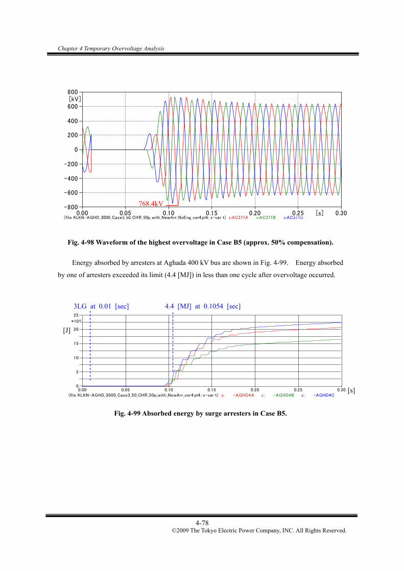
Chapter 4 Temporary Overvoltage Analysis
4-78 ©2009 The Tokyo Electric Power Company, INC. All Rights Reserved.
Fig. 4-98 Waveform of the highest overvoltage in Case B5 (approx. 50% compensation).
Energy absorbed by arresters at Aghada 400 kV bus are shown in Fig. 4-99. Energy absorbed
by one of arresters exceeded its limit (4.4 [MJ]) in less than one cycle after overvoltage occurred.
Fig. 4-99 Absorbed energy by surge arresters in Case B5.
(file KLKN-AGHD_3000_Case3_50_CHR_50p_with_NewArr_NoEng_ver4.pl4; x-var t) v:AC371A v:AC371B v:AC371C 0.00 0.05 0.10 0.15 0.20 0.25 0.30[s]
-800
-600
-400
-200
0
200
400
600
800[kV]
768.4kV
(file KLKN-AGHD_3000_Case3_50_CHR_50p_with_NewArr_ver4.pl4; x-var t) c: -AGHD4A c: -AGHD4B c: -AGHD4C 0.00 0.05 0.10 0.15 0.20 0.25 0.30
0
5
10
15
20
25
*10 6
4.4 [MJ] at 0.1054 [sec]3LG at 0.01 [sec]
[J]
[s]

Chapter 4 Temporary Overvoltage Analysis
4-79 ©2009 The Tokyo Electric Power Company, INC. All Rights Reserved.
4.3.4 Effect of the cable length
In this section, oscillatory overvoltage caused by islanding was calculated with different
lengths of the cable. The switching scenario that led to islanding was assumed to be the one
shown in Fig.4-82. Compensation rates were assumed to be about 100 % as shown in Table 4-27.
Table 4-27 Length of 400 kV Cahir – Aghada Line and Compensation Rates
Shunt reactors [MVA] Length of 400 kV Cahir – Aghada line Aghada Station*1 Cahir
Compensation rate
Base case 112 km 400 560 400 100.7 %
50 % case 56 km 400 --- 300 103.7 %
150 % case 168 km 560 880 600 100.7 %
*1 Shunt reactor station
[50 % case] Length of Cahir - Aghada cable: 56 km
Fig. 4-100 and Fig. 4-101 show the result of the analysis when the length of the 400 kV Cahir
– Aghada cable is 56 km, or half of the base case.
Fig. 4-100 Overvoltage caused by system islanding with 50 % cable length.
645.7 651.9 656.5 659.7 661.5 661.6 660.0
500
550
600
650
700
AC011 AC041 AC071 AC101 AC131 AC161 AC191
Location along the cable
Vol
tage
to th
e ea
rth[
kV_p
eak]
AGHADA CAHIR

Chapter 4 Temporary Overvoltage Analysis
4-80 ©2009 The Tokyo Electric Power Company, INC. All Rights Reserved.
0 2 4 6 8 10[s]-800
-600
-400
-200
0
200
400
600
800[kV]
(file KLKN-AGHD_3000_Case3_50_CHR_0p5ver3.pl4; x-var t) v:AC161A v:AC161B v:AC161C 0.00 0.05 0.10 0.15 0.20 0.25 0.30[s]
-800
-600
-400
-200
0
200
400
600
800[kV]
Fig. 4-101 Waveform of the highest overvoltage with a 50 % cable length.
[150 % case] Length of Cahir - Aghada cable: 168 km
Fig. 4-102 and Fig. 4-103 show the result of the analysis when the length of the 400 kV Cahir
– Aghada cable is 168 km.
Fig. 4-102 Overvoltage caused by System Islanding with 150 % cable length.
590.0
608.9620.9 624.7
637.0 642.1633.7
500
550
600
650
700
AC011 AC101 AC191 AC281 AC371 AC461 AC551
Location along the cable
Vol
tage
to th
e ea
rth[
kV_p
eak]
AGHADA CAHIR
- 661.6kV
Zoom

Chapter 4 Temporary Overvoltage Analysis
4-81 ©2009 The Tokyo Electric Power Company, INC. All Rights Reserved.
0 2 4 6 8 10[s]-800
-600
-400
-200
0
200
400
600
800[kV]
(file KLKN-AGHD_3000_Case3_50_CHR_1p5ver3.pl4; x-var t) v:AC461A v:AC461B v:AC461C 0.00 0.05 0.10 0.15 0.20 0.25 0.30[s]
-800
-600
-400
-200
0
200
400
600
800[kV]
Fig. 4-103 Waveform of the highest overvoltage with 150% cable length.
The effect of the cable length is summarized in Table 4-28. As can be seen from the table,
the effect of the cable length is relatively small.
Table 4-28 Effect of the 400 kV cable length
Length of 400 kV Cahir – Aghada cable
Maximum voltage
Base case 112 km 651.3 kV ( 2.0 p.u.)
50 % case 56 km 661.6 kV ( 2.0 p.u.)
150 % case 168 km 642.1 kV ( 2.0 p.u.)
642.1kV
Zoom

Chapter 4 Temporary Overvoltage Analysis
4-82 ©2009 The Tokyo Electric Power Company, INC. All Rights Reserved.
Fig. 4-104 shows the frequency component spectrum derived from waveforms shown in Fig.
4-101 and Fig. 4-103.
Fig. 4-104 Frequency component spectrum derived from voltage waveforms with different
cable length.
In summary, it was found that load sheddings could cause a very high overvoltage that
exceeded the withstand voltage of a typical 400 kV surge arrester. However, such overvoltage is
not a concern with regards to the safe operation of the network as it can be evaluated using a SIWV
(1050 kV) due to its fast decaying properties.
The overvoltage caused by load shedding was also studied using lower compensation rates.
The overvoltage exceeded SIWV when the compensation rate was 50 %. In addition, the energy
absorbed by the surge arrester exceeded its capability with the compensation rate 50 %. It is
strongly recommended to adopt a compensation rate close to 100 % when the 400 kV Aghada –
Cahir – Kilkenny line is built as an underground cable line as studied in this section.
-50
0
50
100
150
200
250
300
350
400
0 10 20 30 40 50 60 70 80 90 100 110 120 130 140 150
Hz
Vol
tage
[kV
]
50% lengthBase case (100%)150% length

Chapter 4 Temporary Overvoltage Analysis
4-83 ©2009 The Tokyo Electric Power Company, INC. All Rights Reserved.
4.4 Conclusion
The temporary overvoltage analysis was performed based on the compensation pattern
determined by the reactive power compensation analysis. Resonance overvoltages and
overvoltages caused by load shedding were studied with different cable lengths as well as under
different network conditions.
The highest series resonance overvoltage was found in the Woodland 220 kV network. It
was found to be lower than the standard short-duration power-frequency withstand voltage (395 or
460 kV, r.m.s.) specified in IEC 71-1.
The parallel resonance overvoltage was studied with transformer energisation. The observed
overvoltage was much higher than the withstand voltage of a typical 400 kV surge arrester. If the
400 kV Aghada – Cahir – Kilkenny line is built as an underground cable line as studied in this
section, careful study is necessary before energising a transformer at Aghada, Cahir, and Kilkenny.
It is recommended to consider the application of the point-on-wave switching for the transformer
energisation. It has not found its application yet, but the technology itself is already established.
Load sheddings also yielded a very high overvoltage. However, such overvoltage is not a
concern with regards to the safe operation of the network as it can be evaluated using SIWV (1050
kV) due to its fast decaying properties. The overvoltage caused by load shedding was also studied
with lower compensation rates. The overvoltage exceeded SIWV when the compensation rate
was 50 %.
Table 4-29 Summary of the Temporary Overvoltage Analysis
Highest overvoltage
(peak)
Withstand voltage
for evaluation
Series resonance 549.0 kV (3.06 pu) 360, 395, 460 kV (r.m.s.)
(2.83, 3.11, 3.62 pu)
No load 881.5 kV (2.70 pu) Parallel resonance
With load 634.5 kV (1.94 pu)
370 kV (r.m.s.)
(1.60 pu) for 10 seconds
Load shedding 651.3 kV (1.99 pu) 1050 kV (peak)
(r.m.s.) 3
1kV 220or 400 (peak),
3
2kV 220or 400pu 1

Chapter 5 Slow-front Overvoltage Analysis
5-1 ©2009 The Tokyo Electric Power Company, INC. All Rights Reserved.
Chapter 5 Slow-front Overvoltage Analysis
Generally, the overvoltage caused by energisation, de-energisation, fault clearance, and other
switching events is lower for longer cables due to the decay of the overvoltage along the length of
the cable. The overvoltage in the cable is caused by the superimposition of overvoltages reflected
at the both ends of the cable. When the cable has a significant length, the overvoltage would
decay enough by the time it reaches at one end of the cable.
TEPCO has studied switching overvoltages of various lengths of EHV cables, including the
500 kV 39.5 km cable and the 400 kV 106 km cable. The studies did not show any concerns on
the switching overvoltage, particularly due to the significant lengths of the cables.
With this in mind, however, it is a typical practice to study slow-front overvoltages for the
installation of EHV cables. Slow-front overvoltage caused by line energisation, ground fault, and
fault clearing was studied in this chapter for reference. The results of the analysis were evaluated
with SIWV (1050 kV: phase to earth, peak) of 400 kV equipment in NIE and EirGrid.
5.1 Overvoltage Caused by Line Energisation
Overvoltage caused by line energisations was studied by the switching scenarios shown in Fig.
5-1. When one circuit is energised, other circuits are assumed to be out of service as shown in the
figure. This assumption yields the most severe condition for line energisation since the
overvoltage cannot propagate into other circuits.
It was assumed that the time between the line outage and line energisation was long enough to
discharge each cable. The decay time of the residual voltage mainly depends on the X/R ratio of
shunt reactors, and lower X/R ratio means faster decay of the residual voltage. For the typical
X/R ratio of the 400 kV shunt reactors, it can take several minutes to discharge a cable.
Considering this decay time and normal operation practices, it is a common practice to ignore the
residual voltage in the line energisation overvoltage analysis. In addition, the cable will be
discharged through VTs instead of shunt reactors when shunt reactors are not connected to the cable.
In this case, the cable will be discharged within 100 ms.
Line energisations were simulated two hundred times using the statistical switch, in order to
investigate slow-front overvoltages caused by different switching timings.

Chapter 5 Slow-front Overvoltage Analysis
5-2 ©2009 The Tokyo Electric Power Company, INC. All Rights Reserved.
: Open : CloseKilkenny Cahir Aghada
GlanagowOn
Fig. 5-1 Switching scenarios for the overvoltage caused by line energisation.
5.1.1 Overvoltage caused by line energization in the base case
Before simulating the energisation of the 400 kV Cahir – Aghada line, steady state power flow
calculations were conducted under the conditions shown in Fig. 5-2. Source voltages were
adjusted to set the highest voltage along the cable to around 400 kV.
Fig. 5-2 Steady state power flow calculation before simulating line energizations.
Node names are illustrated in Fig. 5-3.
Aghada
AC01 AC07 AC13 AC19 AC25 AC31 AC37 CK01 CK04
Cahir
CK07 CK10 CK13 CK16 CK19
Kilkenny
Fig. 5-3 Node names.
Maximum voltage 400 kV

Chapter 5 Slow-front Overvoltage Analysis
5-3 ©2009 The Tokyo Electric Power Company, INC. All Rights Reserved.
Fig. 5-4 shows the profile of the overvoltage along the 400 kV Aghada – Cahir – Kilkenny line.
The 2 % value in the figure corresponds to the fourth highest overvoltage observed in 200 times
repeated simulations.
Fig. 5-4 The maximum and 2% overvoltage profile in line energisation.
Table 5-1 Maximum Overvoltage along Aghada – Cahir – Kilkenny Line
Aghada - Cahir Cahir - Kilkenny
Voltage Node Voltage Node
Max 564.2kV (1.72 p.u.) AC25 539.8kV (1.65 p.u.) CK07
2% 542.4kV (1.66 p.u.) AC01 518.0kV (1.59 p.u.) CK04, CK07
551.6 552.1 554.9 550.3
564.2554.2
538.9 538.9 538.4 539.8 538.9 537.3 535.4
542.4532.8
527.7520.9 523.9 522.7
514.3 514.3 518.0 518.0 516.2 514.6 510.9 508.5
535.5
450
500
550
600
AC01 AC07 AC13 AC19 AC25 AC31 AC37 CK01 CK04 CK07 CK10 CK13 CK16 CK19
Observing point
Vol
tage
to th
e ea
rth
[kV
] Maximum Value2%Value
Aghada Cahir KilkennyCahir

Chapter 5 Slow-front Overvoltage Analysis
5-4 ©2009 The Tokyo Electric Power Company, INC. All Rights Reserved.
Fig. 5-5 shows the voltage waveform at the Aghada end of the Aghada – Cahir line when the
2 % value 542.4 kV (1.66 pu) was observed in Phase C.
(file KLKN-AGHD_3000_Closing2%.pl4; x-var t) v:AC011A v:AC011B v:AC011C 0 10 20 30 40 50 60 70 80[ms]
-600
-400
-200
0
200
400
600
[kV]
Fig. 5-5 Voltage waveform at the Aghada end of the Aghada - Cahir line
5.1.2 Effect of line length to overvoltage caused by line energization
The slow-front overvoltage caused by line energization was studied with different lengths of
the 400 kV Cahir – Aghada line as shown in Table 5-2. The target frequency of the cable model
(Bergeron model) was adjusted for each case, considering the total cable length between Kilkenny
and Aghada.
Table 5-2 Length of 400 kV Cahir – Aghada Line and Target Frequency of the Cable Model
Reactor compensation [MVA] Length *1 f Target
Aghada Station*2 Cahir
Compensation rate
Base case 112 km 250 Hz 400 560 400 100.7 %
50 % case 56 km 366 Hz 400 --- 300 103.7 %
150 % case 168 km 186 Hz 560 880 600 100.7 %
*1 Length of 400 kV Cahir – Aghada line
*2 Shunt reactor station
542.4kV

Chapter 5 Slow-front Overvoltage Analysis
5-5 ©2009 The Tokyo Electric Power Company, INC. All Rights Reserved.
[50 % case] Length of Cahir – Aghada cable: 56 km
Node names are illustrated in Fig. 5-6.
Fig. 5-6 Node names.
Fig. 5-7 and Table 5-3 show the result of a simulation repeated 200 times.
Fig. 5-7 Profile of the maximum and 2 % value in line energization for a 50 % case.
Table 5-3 Maximum Overvoltage along the Aghada – Cahir – Kilkenny Line for 50 % Case
Aghada – Cahir Cahir – Kilkenny
Voltage Node Voltage Node
Max 531.4 kV (1.63 pu) AC01 515.3 kV (1.58 pu) CK19
2 % 515.5 kV (1.58 pu) AC01 485.1 kV (1.49 pu) CK10
Fig. 5-8 shows the voltage waveform at the Aghada end of the Aghada – Cahir line when the
2 % value 515.5 kV (1.58 pu) was observed in Phase C.
531.4 527.7521.1 518.5
507.6497.2
484.7 484.7 482.8496.4 499.2 504.1 503.1
515.5501.3 498.4 499.5
491.0 487.0
469.7 469.7 474.0483.7 485.1 483.9 484.1 484.9
515.3
400
450
500
550
600
AC01 AC04 AC07 AC10 AC13 AC16 AC19 CK01 CK04 CK07 CK10 CK13 CK16 CK19A
Observing point
Vol
tage
to th
e ea
rth
[kV
] Maximum Value2%Value
Aghada Cahir KilkennyCahir

Chapter 5 Slow-front Overvoltage Analysis
5-6 ©2009 The Tokyo Electric Power Company, INC. All Rights Reserved.
(file KLKN-AGHD_3000_Closing_0p5_2%.pl4; x-var t) v:AC011A v:AC011B v:AC011C 0 10 20 30 40 50 60 70 80[ms]
-600
-400
-200
0
200
400
600[kV]
Fig. 5-8 Voltage waveform at the Aghada end of the Aghada - Cahir line for 50 % case.
[150 % case] Length of Cahir - Aghada cable: 186 km
Node names are illustrated in Fig. 5-9.
Fig. 5-9 Node names.
Fig. 5-10 and Table 5-4 show the result of 200 times repeated simulations.
Fig. 5-10 Profile of the maximum and 2 % value in line energization for 150 % case.
- 515.5kV
536.2 541.7 540.0525.7 521.7 516.0
501.0 501.0 501.9 502.1 500.4 499.0 498.4529.1 534.6 532.2519.6 516.2
507.1491.0 491.0 493.5 495.3 494.9 494.1 491.8 488.7
496.2
400
450
500
550
600
AC01 AC10 AC19 AC28 AC37 AC46 AC55 CK01 CK04 CK07 CK10 CK13 CK16 CK19
Observing point
Vol
tage
to th
e ea
rth
[kV
] Maximum Value2%Value
Aghada Cahir KilkennyCahir

Chapter 5 Slow-front Overvoltage Analysis
5-7 ©2009 The Tokyo Electric Power Company, INC. All Rights Reserved.
Table 5-4 Maximum Overvoltage along the Aghada – Cahir – Kilkenny Line for 150 % Case
Aghada - Cahir Cahir - Kilkenny
Voltage Node Voltage Node
Max 541.7kV (1.66 p.u.) AC10 502.1kV (1.57 p.u.) CK07
2% 534.6kV (1.64 p.u.) AC10 495.3kV (1.52 p.u.) CK07
Fig. 5-8 shows the voltage waveform at the Aghada end of the Aghada – Cahir line when the
2 % value 534.6 kV (1.64 pu) was observed in Phase A.
(file KLKN-AGHD_3000_Closing1p5_2%.pl4; x-var t) v:AC101A v:AC101B v:AC101C 0 10 20 30 40 50 60 70 80[ms]
-600
-400
-200
0
200
400
600[kV]
Fig. 5-11 2% overvoltage waveform at Aghada end of the 400 kV Aghada - Cahir cable when
length of 400 kV Aghada – Cahir cable is 150%
- 534.6kV

Chapter 5 Slow-front Overvoltage Analysis
5-8 ©2009 The Tokyo Electric Power Company, INC. All Rights Reserved.
Fig. 5-12 summarizes the maximum and 2% values for different cable lengths. The observed
overvoltages were much lower than SIWV in all simulated cases, which is typical for long cable
systems.
Fig. 5-12 The maximum and 2% values for different cable lengths.
515.5
542.4534.6
531.4
564.2
541.7
500
520
540
560
580
600
0 20 40 60 80 100 120 140 160 180 200
Length of 400kV cable [km]
Ove
rvol
tage
[kV
]
2%Max

Chapter 5 Slow-front Overvoltage Analysis
5-9 ©2009 The Tokyo Electric Power Company, INC. All Rights Reserved.
5.2 Ground Fault and Fault Clearing Overvoltage
5.2.1 Ground fault and fault clearing overvoltage on the base case
The slow-front overvoltage caused by the ground fault and fault clearing was studied with
different fault timings. The conditions of the analysis are:
Fault point: Seven points in 400 kV Cahir – Kilkenny cable route
Fault type: Single line to ground fault (core to sheath) in Phase A
Fault timing: 0° – 170° (10° step – 18 fault timings)
Fig. 5-13 illustrates the switching scenario for the ground fault and fault clearing overvoltage
analysis.
Fig. 5-13 Switching scenarios for the ground fault and fault clearing overvoltage analysis.
For this analysis, target frequency of all Bergeron models was set to 250 Hz in consideration
of the length of the 400 kV Kilkenny – Cahir – Aghada line. Source impedances were chosen
from short circuit calculation results in summer off-peak demand.
Since the system including 400 kV Cahir – Aghada line is isolated from the main grid after the
tripping of the Kilkenny – Cahir line, the overvoltage in the 400 kV Cahir – Aghada line is similar
to the one caused by load shedding. In general, a smaller model, as in the isolated system, yields a
larger overvoltage due to its lower attenuation and smaller number of propagation routes for the
overvoltage.

Chapter 5 Slow-front Overvoltage Analysis
5-10 ©2009 The Tokyo Electric Power Company, INC. All Rights Reserved.
Fig. 5-14 shows the profile of an overvoltage along the 400 kV Aghada – Cahir – Kilkenny
line. In this analysis, the simulation was repeated 126 times for each case (= 7 fault points × 18
fault timings). Hence, a 2 % value corresponds to the seventh largest value (126 simulations × 3
phases × 0.02) in the simulation at each observation point.
Fig. 5-14 Result of the ground fault and fault clearing analysis.
The maximum value was 542.0 kV (1.66 pu), and the 2 % value was 534.0 kV (1.63 pu),
which were both lower than SIWV.
The 2 % value at the 400 kV Kilkenny bus was observed when the fault occurred at the Cahir
end of the 400 kV Cahir – Kilkenny line at a phase angle of 60. Fig. 5-15 shows the voltage
waveform at this location when the 2 % value was observed.
Fig. 5-15 Overvoltage after the fault clearing of the 400 kV Aghada – Cahir line
(file klkn-aghd_3000_ver3_gc_obs(ac25)_max2%_lg_1_ck01_1 lgs1_a--_140.pl4 ; x-var t) v:AC251A v:AC251B v:AC251C 0.00 0.05 0.10 0.15 0.20 0.25 0.30[s]-600
-400
-200
0
200
400
600[kV]
534.0V Fault timing
526.9535.7 539.0 538.5 542.0 540.9
533.1
417.4 418.1
443.1 436.9452.3
482.0517.5526.4 530.4 530.5 534.0 532.6
524.3
409.7 412.1427.8 427.3
441.0455.7
473.2
500.6
300
350
400
450
500
550
600
AC011A AC071A AC131A AC191A AC251A AC311A AC371A CK011B CK041B CK071C CK101C CK131C CK161B CK191C
Observing point
Vol
tage
[kV
]
M aximum value2% Value
Aghada Cahir KilkennyCahir

Chapter 5 Slow-front Overvoltage Analysis
5-11 ©2009 The Tokyo Electric Power Company, INC. All Rights Reserved.
The highest overvoltage between Kilkenny and Cahir (500.6 kV) was observed at the
Kilkenny 400 kV bus. The overvoltage was caused by the fault in the Cahir 400 kV bus.
(file klkn-aghd_3000_ver3_gc_obs(ck19)_max_lg_1_ck01_1lgs1_a--_110.pl4 ; x-var t) v:CK191A v:CK191B v:CK191C 0.00 0.05 0.10 0.15 0.20 0.25 0.30[s]-600
-400
-200
0
200
400
600[kV]
Fig. 5-16 The highest overvoltage in the Kilkenny 400 kV bus.
5.2.2 Effect of the cable length
In this section, the ground fault and fault clearing overvoltage was studied with different
lengths of the 400 kV Cahir – Aghada line as shown in Table 5-5.
Table 5-5 Length of 400 kV Cahir – Aghada Line
Length of Cahir – Aghada line.
Base case 112 km
150 % case 168 km
50 % case 56 km
- 500.6V
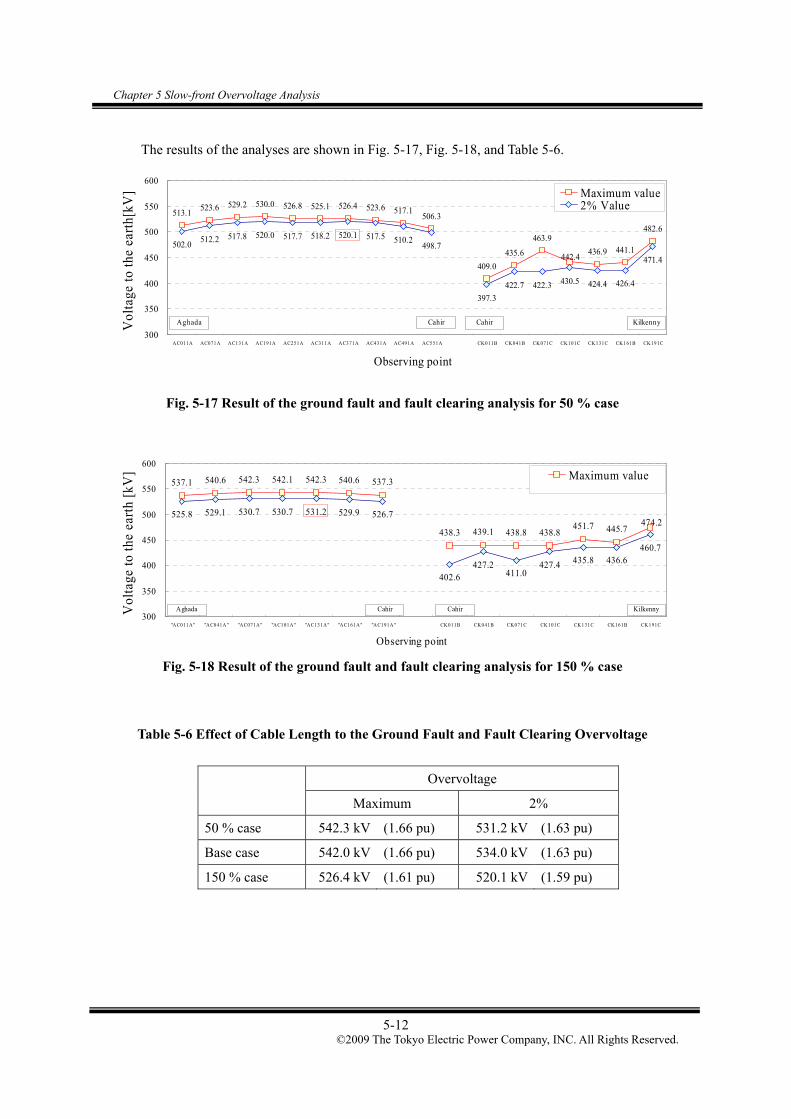
Chapter 5 Slow-front Overvoltage Analysis
5-12 ©2009 The Tokyo Electric Power Company, INC. All Rights Reserved.
The results of the analyses are shown in Fig. 5-17, Fig. 5-18, and Table 5-6.
Fig. 5-17 Result of the ground fault and fault clearing analysis for 50 % case
Fig. 5-18 Result of the ground fault and fault clearing analysis for 150 % case
Table 5-6 Effect of Cable Length to the Ground Fault and Fault Clearing Overvoltage
Overvoltage
Maximum 2%
50 % case 542.3 kV (1.66 pu) 531.2 kV (1.63 pu)
Base case 542.0 kV (1.66 pu) 534.0 kV (1.63 pu)
150 % case 526.4 kV (1.61 pu) 520.1 kV (1.59 pu)
513.1523.6 529.2 530.0 526.8 525.1 526.4 523.6 517.1
506.3
409.0
435.6
463.9
436.9 441.1
482.6
502.0512.2 517.8 520.0 517.7 518.2 520.1 517.5 510.2
498.7
397.3
422.7 422.3 430.5 424.4 426.4
471.4442.4
300
350
400
450
500
550
600
AC011A AC071A AC131A AC191A AC251A AC311A AC371A AC431A AC491A AC551A CK011B CK041B CK071C CK101C CK131C CK161B CK191C
Observing point
Vol
tage
to th
e ea
rth[
kV] Maximum value
2% Value
Aghada Cahir KilkennyCahir
537.1 540.6 542.3 542.1 542.3 540.6 537.3
438.3 439.1 438.8 438.8451.7 445.7
525.8 529.1 530.7 530.7 531.2 529.9 526.7
402.6427.2
411.0427.4 435.8 436.6
460.7
474.2
300
350
400
450
500
550
600
"AC011A" "AC041A" "AC071A" "AC101A" "AC131A" "AC161A" "AC191A" CK011B CK041B CK071C CK101C CK131C CK161B CK191C
Observing point
Vol
tage
to th
e ea
rth
[kV
] Maximum value
Aghada Cahir KilkennyCahir
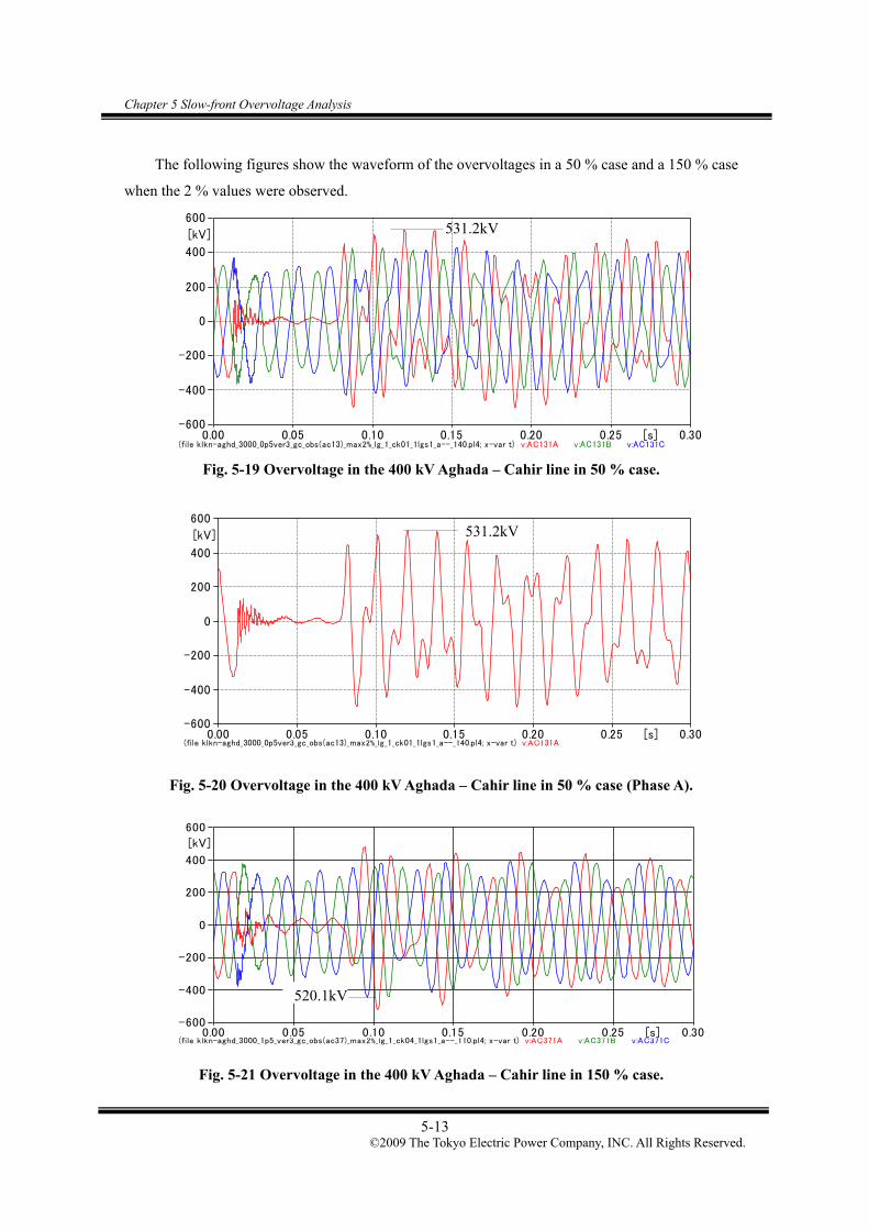
Chapter 5 Slow-front Overvoltage Analysis
5-13 ©2009 The Tokyo Electric Power Company, INC. All Rights Reserved.
The following figures show the waveform of the overvoltages in a 50 % case and a 150 % case
when the 2 % values were observed.
Fig. 5-19 Overvoltage in the 400 kV Aghada – Cahir line in 50 % case.
Fig. 5-20 Overvoltage in the 400 kV Aghada – Cahir line in 50 % case (Phase A).
Fig. 5-21 Overvoltage in the 400 kV Aghada – Cahir line in 150 % case.
(file klkn-aghd_3000_0p5ver3_gc_obs(ac13)_max2%_lg_1_ck01_1lgs1_a--_140.pl4; x-var t) v:AC131A v:AC131B v:AC131C 0.00 0.05 0.10 0.15 0.20 0.25 0.30[s]
-600
-400
-200
0
200
400
600
[kV] 531.2kV
(file klkn-aghd_3000_1p5_ver3_gc_obs(ac37)_max2%_lg_1_ck04_1lgs1_a--_110.pl4; x-var t) v:AC371A v:AC371B v:AC371C 0.00 0.05 0.10 0.15 0.20 0.25 0.30[s]
-600
-400
-200
0
200
400
600
[kV]
520.1kV
(file klkn-aghd_3000_0p5ver3_gc_obs(ac13)_max2%_lg_1_ck01_1lgs1_a--_140.pl4; x-var t) v:AC131A 0.00 0.05 0.10 0.15 0.20 0.25 0.30[s]
-600
-400
-200
0
200
400
600
[kV] 531.2kV

Chapter 5 Slow-front Overvoltage Analysis
5-14 ©2009 The Tokyo Electric Power Company, INC. All Rights Reserved.
Fig. 5-22 Overvoltage in the 400 kV Aghada – Cahir line in 150 % case (Phase A).
The waveform of the overvoltage in Phase A (faulted phase) in the Base case is extracted from
Fig. 5-15 as shown in Fig. 5-23.
Fig. 5-23 Overvoltage in the 400 kV Aghada – Cahir line in Base case (Phase A).
(file klkn-aghd_3000_1p5_ver3_gc_obs(ac37)_max2%_lg_1_ck04_1lgs1_a--_110.pl4; x-var t) v:AC371A 0.00 0.05 0.10 0.15 0.20 0.25 0.30[s]
-600
-380
-160
60
280
500
[kV]
520.1kV
(file klkn-aghd_3000_ver3_gc_obs(ac25)_max2%_lg_1_ck01_1lgs1_a--_140.pl4 ; x-var t) v:AC251A 0.00 0.05 0.10 0.15 0.20 0.25 0.30[s]-600
-400
-200
0
200
400
600[kV]
534.0V

Chapter 5 Slow-front Overvoltage Analysis
5-15 ©2009 The Tokyo Electric Power Company, INC. All Rights Reserved.
Fig. 5-24 shows the result of the Fourier transform performed to the waveforms in Fig. 5-20,
Fig. 5-22, and Fig. 5-23.
Fig. 5-24 Frequency spectrum of the overvoltage for different lengths of the Aghada – Cahir
line.
5.2.3 Effect of the compensation rate
In this section, the ground fault and fault clearing overvoltage was studied with different
compensation rates as shown in Table 5-7 and Fig. 5-25 – Fig. 5-27.
Table 5-7 Compensation Rate of the 400 kV Kilkenny – Cahir – Aghada Line
Locations Case B2 (Base case) Case B4 Case B5
Kilkenny Cahir
100MVA4 80MVA4
100MVA5 80MVA7
100MVA6 80MVA10
Compensation rate of Kilkenny – Cahir line
99.5 [%] 146.6 [%] 193.6 [%]
Cahir Reactor station Aghada
100MVA4 80MVA7 80MVA5
100MVA3 80MVA6 80MVA3
100MVA2 80MVA4 80MVA2
Compensation rate of Cahir - Aghada line 100.7 [%] 75.5 [%] 50.4 [%]
-50
0
50
100
150
200
250
300
350
0 50 100 150 200 250 300 350 400
Frequency [Hz]
Vol
tage
[kV
]
Length 50%Length 100% (Base case)Length 150%

Chapter 5 Slow-front Overvoltage Analysis
5-16 ©2009 The Tokyo Electric Power Company, INC. All Rights Reserved.
Fig. 5-25 Compensation of 400 kV Kilkenny – Cahir – Aghada line in Case B2 (Base case).
Fig. 5-26 Compensation of 400 kV Kilkenny – Cahir – Aghada line in Case B4 (approx. 75 %
compensation).
Fig. 5-27 Compensation of 400 kV Kilkenny – Cahir – Aghada line in Case B5 (approx. 50 %
compensation).
For this analysis, source impedances were decided from short circuit calculation results under
summer off-peak demand.
Kilkenny Cahir AghadaGlanagow
7 points
Close
Trip
100MVAR×4 80MVAR×4 100MVAR
×480MVAR
×780MVAR
×5

Chapter 5 Slow-front Overvoltage Analysis
5-17 ©2009 The Tokyo Electric Power Company, INC. All Rights Reserved.
The profile of the overvoltage in Cases B4 and B5 are shown in Fig. 5-28 and Fig. 5-29.
Fig. 5-28 Result of the ground fault and fault clearing analysis in Case B4 (approx. 75 %
compensation).
Fig. 5-29 Result of the ground fault and fault clearing analysis in Case B5 (approx. 50 %
compensation).
Effects of the compensation rates are summarized in Table 5-8. A lower compensation rate
yields higher overvoltage, but the observed overvoltage was much lower than SIWV.
Table 5-8 Effect of Compensation Rate
Over voltage
Maximum 2 %
Case B2 (approx. 100 % compensation) 542.3 kV (1.66 pu) 531.2 kV (1.63 pu)
Case B4 (approx. 75 % compensation) 593.3 kV (1.82 pu) 585.7 kV (1.79 pu)
Case B5 (approx. 50 % compensation) 692.7 kV (2.12 pu) 678.4 kV (2.08 p.u.)
675.1 687.2 692.7 692.4 692.5 686.7 675.3
406.5 406.6428.5 422.5
438.8464.2
657.5670.0 676.1 677.5 678.4 674.6 664.0
386.7 389.7416.4 412.9
426.1439.3
455.8
481.4
300
400
500
600
700
800
AC011A AC071A AC131A AC191A AC251A AC311A AC371A CK011B CK041B CK071C CK101C CK131C CK161B CK191C
Observing point
Vol
tage
to th
e ea
rth
[kV
_pea
k]
M aximum Value2% Value
Aghada Cahir KilkennyCahir
579.2 589.0 593.3 592.5 593.0 590.4 582.2
414.1 414.5438.0 431.8
447.9475.4
573.6 581.8 585.2 583.2 585.7 582.6 573.8
394.0 397.7424.4 422.1 435.1
449.7467.3
493.4
300
400
500
600
700
AC011A AC071A AC131A AC191A AC251A AC311A AC371A CK011B CK041B CK071C CK101C CK131C CK161B CK191C
Observing point
Vol
tage
to th
e ea
rth
[kV
_pea
k]
M aximum Value2% Value
Aghada Cahir KilkennyCahir
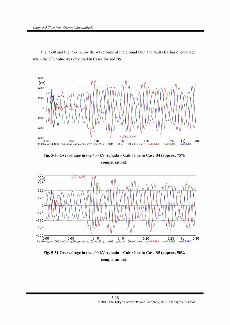
Chapter 5 Slow-front Overvoltage Analysis
5-18 ©2009 The Tokyo Electric Power Company, INC. All Rights Reserved.
Fig. 5-30 and Fig. 5-31 show the waveforms of the ground fault and fault clearing overvoltage
when the 2 % value was observed in Cases B4 and B5.
Fig. 5-30 Overvoltage in the 400 kV Aghada – Cahir line in Case B4 (approx. 75%
compensation).
Fig. 5-31 Overvoltage in the 400 kV Aghada – Cahir line in Case B5 (approx. 50%
compensation).
(file klkn-aghd_3000_ver3_chag_50p_gc_obs(ac25)_max2%_lg_1_ck07_1lgs1_a--_100.pl4; x-var t) v:AC251A v:AC251B v:AC251C 0.00 0.05 0.10 0.15 0.20 0.25 0.30[s]
-700
-525
-350
-175
0
175
350
525
700[kV]
678.4kV
(file klkn-aghd_3000_ver3_chag_75p_gc_obs(ac25)_max2%_lg_1_ck04_1lgs1_a--_100.pl4; x-var t) v:AC251A v:AC251B v:AC251C 0.00 0.05 0.10 0.15 0.20 0.25 0.30[s]
-600
-400
-200
0
200
400
600
[kV]
- 585.7kV

Chapter 5 Slow-front Overvoltage Analysis
5-19 ©2009 The Tokyo Electric Power Company, INC. All Rights Reserved.
5.2.4 Effect of source impedance
The effect of source impedance to the ground fault and fault clearing overvoltage was studied
with the source impedance values shown in Table 5-9.
Table 5-9 Assumed Sets of Source Impedance Values
Kilkenny 220 kV Cahir 110 kV Aghada 220 kV
Case 1 50 mH 15 mH 20 mH
Case 2 75 mH 20 mH 55 mH
Case 3 100 mH 25 mH 90 mH
Results of the analysis in Case 1, Case 2 and Case 3 are shown in Fig. 5-32 – Fig. 5-34.
Fig. 5-32 Result of the ground fault and fault clearing analysis in Case 1
529.0 541.0 546.3 546.5 550.0 549.5 541.2
421.6 422.3446.0 440.8
457.6 468.3519.3
531.8 537.8 538.0 541.2 539.7 530.5
404.8 406.3429.9 423.6
438.4455.9
471.9
483.8
300
400
500
600
700
AC011A AC071A AC131A AC191A AC251A AC311A AC371A CK011B CK041B CK071C CK101C CK131C CK161B CK191C
Observing point
Vol
tage
to th
e ea
rth
[kV
_pea
k] Maximum Value2% Value
Aghada Cahir KilkennyCahir
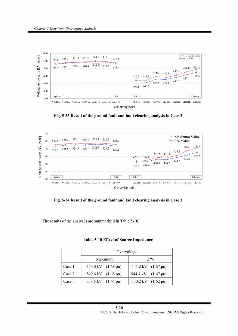
Chapter 5 Slow-front Overvoltage Analysis
5-20 ©2009 The Tokyo Electric Power Company, INC. All Rights Reserved.
Fig. 5-33 Result of the ground fault and fault clearing analysis in Case 2
Fig. 5-34 Result of the ground fault and fault clearing analysis in Case 3
The results of the analyses are summarized in Table 5-10.
Table 5-10 Effect of Source Impedance
Overvoltage
Maximum 2 %
Case 1 550.0 kV (1.68 pu) 541.2 kV (1.67 pu)
Case 2 549.6 kV (1.68 pu) 544.7 kV (1.67 pu)
Case 3 538.5 kV (1.65 pu) 530.2 kV (1.62 pu)
529.0 538.3 541.5 544.6 549.6 547.1 537.1
420.9 421.1445.7 439.8
455.6476.8525.7 535.4 540.6 540.4 544.7 542.9 534.6
404.1 406.2428.6 427.1
439.7457.1
475.6
495.2
300
350
400
450
500
550
600
AC011A AC071A AC131A AC191A AC251A AC311A AC371A CK011B CK041B CK071C CK101C CK131C CK161B CK191C
Observing point
Vol
tage
to th
e ea
rth
[kV
_pea
k] M aximum Value2% Value
Aghada Cahir KilkennyCahir
527.8 535.2 538.1 536.4 538.5 536.7 528.7
421.3 422.8444.0 441.4
458.5
488.0517.7 525.5 528.5 526.7 530.2 528.2 520.2
414.4 416.4430.8 430.7
444.5459.1
476.3
506.8
300
350
400
450
500
550
600
AC011A AC071A AC131A AC191A AC251A AC311A AC371A CK011B CK041B CK071C CK101C CK131C CK161B CK191C
Observing point
Vol
tage
to th
e ea
rth
[kV
_pea
k] Maximum Value2% Value
Aghada Cahir KilkennyCahir

Chapter 5 Slow-front Overvoltage Analysis
5-21 ©2009 The Tokyo Electric Power Company, INC. All Rights Reserved.
Fig. 5-35 – Fig. 5-37 shows the waveforms of the ground fault and fault clearing overvoltage
when the 2 % values were observed in Cases 1, 2 and 3.
(file klkn-aghd_3000_ver3_gen_max_gc_obs(ac25)_max2%_lg_1_ck04_1lgs1_a--_100.pl4; x-var t) v:AC251A v:AC251B v:AC251C 0.00 0.05 0.10 0.15 0.20 0.25 0.30[s]
-600
-400
-200
0
200
400
600
[kV]
Fig. 5-35 Overvoltage in the 400 kV Aghada – Cahir line in Case 1.
(file klkn-aghd_3000_ver3_gen_middle_gc_obs(ac25)_max2%_lg_1_ck01_1lgs1_a--_040.pl4; x-var t) v:AC251A v:AC251B v:AC251C 0.00 0.05 0.10 0.15 0.20 0.25 0.30[s]
-600
-400
-200
0
200
400
600
[kV]
Fig. 5-36 Overvoltage in the 400 kV Aghada – Cahir line in Case 2.
- 541.2kV
544.7kV

Chapter 5 Slow-front Overvoltage Analysis
5-22 ©2009 The Tokyo Electric Power Company, INC. All Rights Reserved.
(file klkn-aghd_3000_ver3_gen_min_gc_obs(ac25)_max2%_lg_1_ck04_1lgs1_a--_080.pl4; x-var t) v:AC251A v:AC251B v:AC251C 0.00 0.05 0.10 0.15 0.20 0.25 0.30[s]
-600
-400
-200
0
200
400
600
[kV]
Fig. 5-37 Overvoltage in the 400 kV Aghada – Cahir line in Case 3.
In this section, the overvoltage caused by line energisation was studied with different
conditions. The observed overvoltages were much lower than SIWV in all simulated cases, which
is typical for long cable systems.
5.3 Conclusion
Slow-front overvoltage caused by line energisation, ground fault, and fault clearing was
studied in this chapter. The result of the slow-front overvoltage analysis is summarized in Table
5-11. As shown in the table, no significant overvoltage was found in the slow-front overvoltage
analysis. The observed overvoltages were much lower than SIWV in all simulated cases.
Table 5-11 Summary of the Slow-front Overvoltage Analysis
Highest overvoltage
(peak)
Withstand voltage (peak)
for evaluation
Line energisation 564.2 kV (1.72 pu)
Ground fault and fault clearing 692.7 kV (2.12 pu) 1050 kV
(peak) 3
2kV 400pu 1
530.2kV

Chapter 6 Voltage Stability / Variation
6-1 ©2009 The Tokyo Electric Power Company, INC. All Rights Reserved.
Chapter 6 Voltage Stability / Variation
Depending on the reactive power compensation rate of the cable, the loss of the 400 kV cable
can cause large voltage variation or voltage instability. Voltage stability and variation caused by
the loss of the long 400 kV cable was studied in this chapter.
Long cables for the study of voltage stability and variation are shown in Table 6-1. Reactive
power compensation rates of the cables were varied from 70 % to 100 % in 10 % steps.
Table 6-1 List of Cables for the Study of Voltage Stability and Variation
KV From Bus To Bus Charging
[MVA/cct]
Length
[km]
3774 KINGSCOURT 90140 TURL 762.3 82
3774 KINGSCOURT 5464 WOODLAND 539.2 58 400
1044 AGHADA 1724 CAHIR 1350.2 112
6.1 Voltage Variation by the Loss of the 400 kV Cable
The following voltage variation is allowed in the operation of the all-island transmission
system.
Under normal operating conditions: 3 % (11.4 kV)
Under contingencies: 10 % (38.0 kV)
As the most severe condition, the power flow data in summer off-peak demand and in winter
peak demand with maximum wind were selected for the analysis of the voltage variation. In this
power flow data, a cable and shunt reactors connected directly to the cable were switched off to
find the voltage variation caused by the loss of the 400 kV cable. Reactive power compensation
rates of the cables were varied from 70 % to 100 % in 10 % steps. Fig. 6-1 shows the voltage
variation by the loss of the 400 kV Kingscourt – Turleenan line in winter peak demand with
maximum wind. In Fig. 6-1, positive values of voltage variation indicate a voltage drop.

Chapter 6 Voltage Stability / Variation
6-2 ©2009 The Tokyo Electric Power Company, INC. All Rights Reserved.
-0.005
0.000
0.005
0.010
0.015
0.020
0.025
0.030
60 70 80 90 100 110
Compensation Rate [%]
Vol
tage
Var
iatio
n [p
u TURL 400
KINGSCOURT 400
WOODLAND 400
FLAGFORD 400
TURL 275
KINGSCOURT 220
Fig. 6-1 Voltage variation by the loss of the 400 kV Kingscourt – Turleenan line in winter peak demand with maximum wind.
From Fig. 6-1, it can be seen that the voltage variation is kept within 10 %.
Next, the same analysis was performed in the summer off-peak demand. The result of the
analysis is shown in Fig. 6-2.
-0.005
0.000
0.005
0.010
0.015
0.020
0.025
0.030
60 70 80 90 100 110
Compensation Rate [%]
Vol
tage
Var
iatio
n [p
u TURL 400
KINGSCOURT 400
WOODLAND 400
FLAGFORD 400
TURL 275
KINGSCOURT 220
Fig. 6-2 Voltage variation with the loss of the 400 kV Kingscourt – Turleenan line in the summer off-peak demand.

Chapter 6 Voltage Stability / Variation
6-3 ©2009 The Tokyo Electric Power Company, INC. All Rights Reserved.
From Fig. 6-2, it can be seen that there is no problem in the voltage variation also in the
summer off-peak demand.
The same analysis was performed for the 400 kV Woodland – Kingscourt line in the winter
peak demand with maximum wind. The results of the analysis are shown in Fig. 6-3.
-0.005
0.000
0.005
0.010
0.015
0.020
0.025
0.030
60 70 80 90 100 110
Compensation Rate [%]
Vol
tage
Var
iatio
n [p
u TURL 400
KINGSCOURT 400
WOODLAND 400
FLAGFORD 400
OLDSTREE 400
MAYNOOTH 400
Fig. 6-3 Voltage variation by the loss of 400 kV Woodland – Kingscourt line in winter peak
demand with maximum wind.
From Fig. 6-3, it can be seen that the voltage variation is maintained within 10 %.
The same analysis was performed in the summer off-peak demand. The result of the analysis
is shown in Fig. 6-4.

Chapter 6 Voltage Stability / Variation
6-4 ©2009 The Tokyo Electric Power Company, INC. All Rights Reserved.
-0.005
0.000
0.005
0.010
0.015
0.020
0.025
0.030
60 70 80 90 100 110
Compensation Rate [%]
Vol
tage
Var
iatio
n [p
u TURL 400
KINGSCOURT 400
WOODLAND 400
FLAGFORD 400
OLDSTREE 400
MAYNOOTH 400
Fig. 6-4 Voltage variation with the loss of the 400 kV Woodland – Kingscourt line in summer off-peak demand.
From Fig. 6-4, it can be seen that there is no problem in the voltage variation.
The same analysis was performed for the 400 kV Cahir – Aghada line in the winter peak
demand with maximum wind. The results of the analysis are shown in Fig. 6-5.
-0.02
0.00
0.02
0.04
0.06
0.08
0.10
0.12
60 70 80 90 100 110
Compensation Rate [%]
Vol
tage
Var
iatio
n [p
u
KILKENNY 220
KILKENNY 380
CAHIR 380
AGHADA 380
AGHADA 220
Fig. 6-5 Voltage variation with the loss of the 400 kV Cahir – Aghada line in winter peak demand with maximum wind.

Chapter 6 Voltage Stability / Variation
6-5 ©2009 The Tokyo Electric Power Company, INC. All Rights Reserved.
From Fig. 6-5, it can be seen that there is no problem in the voltage variation. Aghada 220
kV bus voltage is maintained at a constant voltage by reactive power supply from neighboring
generators.
Next, the same analysis was performed in the summer off-peak demand. The result of the
analysis is shown in Fig. 6-6.
-0.02
0.00
0.02
0.04
0.06
0.08
0.10
0.12
60 70 80 90 100 110
Compensation Rate [%]
Vol
tage
Var
iatio
n [p
u
KILKENNY 220
KILKENNY 380
CAHIR 380
AGHADA 380
AGHADA 220
Fig. 6-6 Voltage Variation with the Loss of Cahir – Aghada 400 kV Line in Summer Off-Peak
Demand.
From Fig. 6-6, when the compensation rate is 70 %, the voltage variation of the Aghada 380
kV bus exceeds 10 %. In all other cases, it was found that there was no problem in the voltage
variation.

Chapter 6 Voltage Stability / Variation
6-6 ©2009 The Tokyo Electric Power Company, INC. All Rights Reserved.
6.2 Voltage Stability with the Loss of the 400 kV Cable
As the most severe condition, power flow data in the winter peak demand with maximum
wind was selected for the analysis of the voltage stability. In this power flow data, the 400 kV
cables in Table 6-1 and shunt reactors connected directly to the cables were switched off in order to
study the voltage stability of the system with the loss of the 400 kV cable. Reactive power
compensation rates of the 400 kV cables were varied from 70 % to 100 % by 10 % steps. In order
to increase the power flow of N-S interconnectors by 1500MW, generators in the power flow data
were dispatched as shown Table 6-2. In this analysis controls of tap changers and switched shunt
capacitors/reactors were blocked. Fig. 6-7 shows PV curves at the Kingscourt 400 kV bus with
the loss of the 400 kV Kingscourt – Turleenan line.
Table 6-2 Generators Dispatched to Increase the Power Flow of N-S Interconnectors
Generators increased output Generators decreased output
Number Name Output Number Name Output
70504 BAFDG4 0→168 39471 MNYPG1 285.2→115
70505 BAFDG5 0→168 39472 MNYPG2-P 285.2→115
70506 BAFDG6 0→168 39473 MNYPG3 285.2→115
70520 BAFD2- 0→400 50573 SEAL ROC 81.4→0
74520 CAST2- 0→400 50574 SEAL ROC 81.4→0
86225 BALLYCRO 425→500 44471 POLLG1_4 15→5
70515 BAFD_GC 189→200 44471 POLLG1_4 15→5
82001 KILRG1- 226→300 44471 POLLG1_4 4→1
82002 KILRG2- 227→300 28571 GLANAGOW 405→110.1
35771 LONGPOIN 408→222
31271 DUBLIN B 395.6→163
29673 HUNTSTOW 308→257
49474 WOP_G4 150→55

Chapter 6 Voltage Stability / Variation
6-7 ©2009 The Tokyo Electric Power Company, INC. All Rights Reserved.
0.950
0.970
0.990
1.010
1.030
1.050
1.070
0 200 400 600 800 1000 1200 1400 1600
Increment Transfer [MW]
Bus
Vol
tage
[kV
]
Rate_100%
Rate_90%
Rate_80%
Rate_70%
Fig. 6-7 PV-curves at the Kingscourt 400 kV bus with the loss of the 400 kV Kingscourt – Turleenan line.
The voltage stability was maintained even after the power flow in the N-S interconnectors was
increased by 1500 MW as shown in Fig. 6-7.
Next, the same analysis was performed at the Woodland 400 kV bus with the loss of the 400
kV Woodland – Kingscourt line. The result of the analysis is shown in Fig. 6-8.
0.950
0.970
0.990
1.010
1.030
1.050
1.070
0 200 400 600 800 1000 1200 1400 1600
Increment Transfer [MW]
Bus
Vol
tage
[kV
]
Rate_100%
Rate_90%
Rate_80%
Rate_70%
Fig. 6-8 PV-curves at the Woodland 400 kV bus with the loss of the 400 kV Woodland – Kingscourt line.

Chapter 6 Voltage Stability / Variation
6-8 ©2009 The Tokyo Electric Power Company, INC. All Rights Reserved.
The voltage stability was maintained even after the power flow in the N-S interconnectors
were increased by 1500 MW as shown in Fig. 6-8.
The loss of the 400 kV Cahir – Aghada line leads to the loss of reactive power supply to the
Cahir 400 kV and 110 kV network. In order to determine the ability of a power system to
maintain voltage stability at the Cahir 400 kV bus, the loads and generators in the power flow data
were dispatched as shown Table 6-3. In this analysis controls of tap changers and switched shunt
capacitors/reactors were blocked.
The result of the analysis is shown in Fig. 6-9.
Table 6-3 Loads and Generators Dispatched to Increase the Power Flow of the 400 kV
Kilkenny - Cahir Line
generators increased output Increased loads
Number Name Output Area
number Area name
Total base
Load (=1.0pu)
70504 BAFDG4 0→168 3 CORK KERRY 911.2MW
70505 BAFDG5 0→168 5 CAHIR NETW 554.5MW
70506 BAFDG6 0→168
70520 BAFD2- 0→400
74520 CAST2- 0→400

Chapter 6 Voltage Stability / Variation
6-9 ©2009 The Tokyo Electric Power Company, INC. All Rights Reserved.
0.86
0.88
0.90
0.92
0.94
0.96
0.98
1.00
1.02
1.04
1.06
1.00 1.10 1.20 1.30 1.40 1.50 1.60 1.70 1.80
Active Power [pu]
Bus
Vol
tage
[kV
]
Rate_100%
Rate_90%
Rate_80%
Rate 70%
Fig. 6-9 PV-curves at the Cahir 400 kV bus with the loss of the 400 kV Cahir - Aghada line.
The voltage stability was maintained even after the winter peak demand was increased to
150% as shown in Fig. 6-9.
As the most severe condition, the same analysis was performed under outages of generators at
Glanagow and Longpoint. In order to adjust the demand-supply balance, outputs of some
generators in the power flow data were changed as shown in Table 6-4. The result of the analysis
is shown in Fig. 6-10.
Table 6-4 Generators Dispatched to Adjust Demand-Supply
Number Name Output
29671 HUNT_ST 0→120
29672 HUNT_CT 0→230
39471 MNYPG1 285.2→301.5
39472 MNYPG2-P 285.2→301.5
39473 MNYPG3 285.2→301.5
44671 PBEGG1 0→115
44672 PBEGG2 0→115
44673 PBEGG3 0→255

Chapter 6 Voltage Stability / Variation
6-10 ©2009 The Tokyo Electric Power Company, INC. All Rights Reserved.
0.88
0.90
0.92
0.94
0.96
0.98
1.00
1.02
1.04
1.06
1.00 1.10 1.20 1.30 1.40 1.50
Active Power [pu]
Bus
Vol
tage
[kV
]
Rate_100%
Rate_90%
Rate_80%
Rate 70%
Fig. 6-10 PV-curves at the Cahir 400 kV bus with the loss of the 400 kV Cahir - Aghada line
under outages of generators at Glanagow and Longpoint.
The voltage stability was maintained even after the winter peak demand was increased to
125 % as shown in Fig. 6-10.

Chapter 6 Voltage Stability / Variation
6-11 ©2009 The Tokyo Electric Power Company, INC. All Rights Reserved.
6.3 Conclusion
Depending on the reactive power compensation rate of the cable, the loss of the 400 kV cable
can cause large voltage variation or voltage instability. Voltage stability and variation caused by
the loss of the long 400 kV cable was studied in this chapter.
In the voltage variation analysis, the losses of the 400 kV Kingscourt – Turleenan line, the 400
kV Woodland – Kingscourt line, and the 400 kV Cahir – Aghada line were studied in winter peak
demand with maximum wind and in summer off-peak demand. The reactive power compensation
rates were varied from 70 % to 100 % by 10 % step. The variation above 10 % was observed in
the loss of the 400 kV Cahir – Aghada line in summer off-peak demand. Since the violation
occurred when the compensation rate was 70 %, the compensation rate of the 400 kV Cahir –
Aghada line has to be higher than 70 % in order to comply with the transmission planning criteria.
In the voltage stability analysis, the losses of the 400 kV Kingscourt – Turleenan line, the 400
kV Woodland – Kingscourt line, and the 400 kV Cahir – Aghada line were studied in winter peak
demand with maximum wind. As in the voltage variation analysis, the reactive power
compensation rates were varied from 70 % to 100 % by 10 % step. It was confirmed that the
voltage stability was maintained after increasing the power flow in the N-S interconnectors or the
winter peak demand within the reasonable range.

Chapter 7 Black-start Capability
7-1 ©2009 The Tokyo Electric Power Company, INC. All Rights Reserved.
Chapter 7 Black-start Capability
In the restoration of the bulk power system, sustained power frequency overvoltages may be
caused by charging current. When the restoration has to be realized through an EHV underground
cable with significant length, black-start generators would be required to have sufficient
under-excitation capability, depending on the compensation rate of the cable charging capacity.
Besides the sustained power frequency overvoltages, harmonic resonance overvoltage can be
caused in the restoration of the bulk power system. The highest concern is the second harmonic
current injection as in the parallel resonance overvoltage analysis. In the restoration through the
network largely composed of OHTLs, it is generally possible to avoid the resonance condition by
the connection of generators and loads and/or other operational measures. For the network largely
composed of EHV underground cables, it requires careful assessment when establishing restoration
procedures.
The analysis needs to be performed both on under-excitation capability of black-start
generators and on harmonic resonance overvoltage. The blackout restoration procedures of NIE
and EirGrid are evaluated after replacing some OHLs by underground cables.

Chapter 7 Black-start Capability
7-2 ©2009 The Tokyo Electric Power Company, INC. All Rights Reserved.
7.1 Restoration in the Eirgrid Network
This section has been deleted due to the security concerns for the EirGrid Network.

Chapter 7 Black-start Capability
7-3 ©2009 The Tokyo Electric Power Company, INC. All Rights Reserved.
7.2 Restoration in the NIE Network
The northwest area was selected for the black-start capability study because 275 kV
Coolkeeragh – Strabane – Omagh line was replaced by underground cables.
7.2.1 Restoration procedure
The restoration procedure is shown in Fig. 7-1.

Chapter 7 Black-start Capability
7-4 ©2009 The Tokyo Electric Power Company, INC. All Rights Reserved.
Fig. 7-1 Restoration procedure.
7.2.2 Under-excitation capability of black-start generators
In order to find the effect of the installation of cables on the ability to black-start, power flow
calculations were conducted in PSS/E under both OHL and cable conditions for the lines shown in
Table 7-1. Compensation rate of the Coolkeeragh – Strabane – Omagh cable was set to be 100 %.
Table 7-1 List of OHLs Replaced by Cables
Original
Impedance/Susceptance
Modified
Impedance/Susceptance KV
From
Bus
Name
To Bus
Name Line R
(pu)
Line X
(pu)
Charging
(pu)
Line R
(pu)
Line X
(pu)
Charging
(pu)
COOLKEE
STRABANE 0.00126 0.01041 0.06755 0.000789 0.007978 1.3045 275
OMAH STRABANE 0.00151 0.0125 0.08106 0.001894 0.019146 3.1308
As the most severe condition, generators and loads in the power flow data were dispatched as
shown Table 7-2 and Table 7-3, respectively. In this analysis, it was assumed that one
transmission line and one transformer were in service, shunt capacitors were out of service, and
generator terminal voltage was controlled at the rated voltage.

Chapter 7 Black-start Capability
7-5 ©2009 The Tokyo Electric Power Company, INC. All Rights Reserved.
Table 7-2 Outputs of Generators for Black-start Analysis
Generator Voltage[kV] Pg[MW] Pgmax[MW] Pgmin[MW]
COOL_GT 16.0 20 259 20
COOL_ST 16.0 30 136 30
OCGT 11.0 13.75 55 0
Table 7-3 Loads for Black-start Analysis
Bus name Voltage[kV] PL[MW] QL[MVar]
COOLG8 33.0 37.2 30.8
LSMR3 33.0 26.6 22.0
The result of the analysis is shown in Table 7-4. It can be seen from the table that under both
OHL and cable conditions, outputs of generators are kept within the generator reactive capability
limitation. In the case of OHL, output of each generator decreases; in the case of the cable, output
of each generator is kept at a constant value because of 100 % compensation. Note that the
negative Qgen in the figure means the generator is absorbing reactive power.
Table 7-4 Reactive power from Coolkeeragh power staton.
Qgen[Mvar]
OHL Cable Bus name
Step1 Step2 Step3 Step1 Step2 Step3
Qgmax
[MVar]
Qgmin
[MVar]
COOL_GT 10.6 5.7 -0.3 10.6 10.6 10.6 120 -60
COOL_ST 40.5 38.5 36.2 40.5 40.5 40.5 70 -40
OCGT 13.0 12.5 11.9 13.0 13.0 13.0 50 -16
Then, in order to find the effect of the compensation rate of the Coolkeeragh – Strabane –
Omagh line, the same analysis was performed with different compensation rates 70 % and 85 %.

Chapter 7 Black-start Capability
7-6 ©2009 The Tokyo Electric Power Company, INC. All Rights Reserved.
The result of the analysis at Step 2 is shown in Fig. 7-2. The horizontal axis of the figure
shows the compensation rate of the 275 kV Coolkeeragh – Strabane line. It can be seen from the
figures that outputs of generators are kept within the generator reactive capability limitation in this
step.
-80
-60
-40
-20
0
20
40
60
80
100
120
140
70% 75% 80% 85% 90% 95% 100%
Compensation Rate [%]
Qgen [MVar]
COOL_GT
Qmax (MVAR)
Qmin (MVAR)
Reactive power from GT
-60
-40
-20
0
20
40
60
80
70% 75% 80% 85% 90% 95% 100%
Compensation Rate [%]
Qgen [MVar]
COOL_ST
Qmax (MVAR)
Qmin (MVAR)
Reactive power from ST
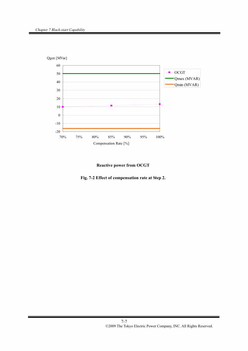
Chapter 7 Black-start Capability
7-7 ©2009 The Tokyo Electric Power Company, INC. All Rights Reserved.
-20
-10
0
10
20
30
40
50
60
70% 75% 80% 85% 90% 95% 100%
Compensation Rate [%]
Qgen [MVar]
OCGT
Qmax (MVAR)
Qmin (MVAR)
Reactive power from OCGT
Fig. 7-2 Effect of compensation rate at Step 2.

Chapter 7 Black-start Capability
7-8 ©2009 The Tokyo Electric Power Company, INC. All Rights Reserved.
The result of the analysis at Step 3 is shown in Fig. 7-3. The horizontal axis of the figure
shows the compensation rate of the 275 kV Strabane – Omagh line, and lines with different colors
show the compensation rate of the 275 kV Coolkeeragh – Strabane. It can be seen from the
figures that outputs of ST and OCGT are kept within the generator reactive capability limitation,
but those of GT exceed the limitation with lower compensation rates. Note that negative Qgen in
the figure means the generator is absorbing reactive power.
-150
-100
-50
0
50
100
150
70% 75% 80% 85% 90% 95% 100%
Compensation Rate [%]
Qgen [MVar]
CK-ST 100%
CK-ST 85%
CK-ST 70%
Qmax (MVAR)
Qmin (MVAR)
Reactive power from GT
-60
-40
-20
0
20
40
60
80
70% 75% 80% 85% 90% 95% 100%
Compensation Rate [%]
Qgen [MVar]
CK-ST 100%
CK-ST 85%
CK-ST 70%
Qmax (MVAR)
Qmin (MVAR)
Reactive power from ST

Chapter 7 Black-start Capability
7-9 ©2009 The Tokyo Electric Power Company, INC. All Rights Reserved.
-20
-10
0
10
20
30
40
50
60
70% 75% 80% 85% 90% 95% 100%
Compensation Rate [%]
Qgen [MVar] CK-ST 100%
CK-ST 85%
CK-ST 70%
Qmax (MVAR)
Qmin (MVAR)
Reactive power from OCGT
Fig. 7-3 Effect of compensation rate at Step 3.
Fig. 7-4 shows the busbar voltage at the Omagh 275 kV with different compensation rates. It
can be seen from the figures that busbar voltages exceed 300 kV for lower compensation rates.
275.0
280.0
285.0
290.0
295.0
300.0
305.0
310.0
70% 75% 80% 85% 90% 95% 100%
Compensation Rate [%]
Busbar Voltage [KV]
OMA_CK-ST 100%
OMA_CK-ST 85%
OMA_CK-ST 70%
Fig. 7-4 Busbar voltage at Omagh 275kV with different compensation rates at Step 3.

Chapter 7 Black-start Capability
7-10 ©2009 The Tokyo Electric Power Company, INC. All Rights Reserved.
7.2.3 Parallel resonance frequency
Parallel resonance frequency of the network was found by frequency scan using the simulation
model in Fig. 7-5
CLKR 275 #1
X0020SAT
Y Y
CLKR_LB
CLKLBSAT
Y Y
LSMR_#1
LSMR1 LSMR3SAT
Y Y
CLKR_ST
CLKRSSAT
Y Y
CABLE_OM-ST
CLKR_GT
CLKRTSAT
Y Y
OHL_CL-LS
100%100%
CABLE_ST-CL
1A
37.2+j30.8CLKLB
100%
26.LSMR3
100%
0.652L-89.6
V
CLKR_8G
CLKR8SAT
Y Y
Fig. 7-5 Simulation model for frequency sweep.
First, the result of frequency scan seen from Coolkeeragh 275 kV at Step 1 is shown in Fig.
7-6. As in the frequency scan result seen from Coolkeeragh 275 kV, the highest peak was found
at 3254 Hz.
Current source
(1 Amp)
Coolkeeragh p/s Omagh – Strabane line
Strabane – Coolkeeragh line

Chapter 7 Black-start Capability
7-11 ©2009 The Tokyo Electric Power Company, INC. All Rights Reserved.
(file fs_ni_step1.pl4; x-var f) v:X0021A v:X0021B v:X0021C 0 1000 2000 3000 4000 5000[Hz]
0
40
80
120
160
200
[kΩ]
Fig. 7-6 Parallel resonance frequency of the network seen from Coolkeeragh 275 kV at Step
1.
3254Hz-165kΩ

Chapter 7 Black-start Capability
7-12 ©2009 The Tokyo Electric Power Company, INC. All Rights Reserved.
Next, in order to find the effect of the replacement of OHLs by cables on the resonance
frequency, a frequency scan was conducted under both OHL and cable conditions. In this analysis,
the compensation rate of shunt reactor was set to be 100 %.
The results of frequency scan are shown in Fig. 7-7. It can be seen that parallel resonance
frequency was shifted to lower frequency and the magnitude of impedance at parallel resonance
decreased when 275 kV Strabane – Coolkeeragh line was replaced by cables.
fs_ni_step2_ohl.pl4: v:X0021A fs_ni_step2_sc100.pl4: v:X0021A
0 200 400 600 800 1000[Hz]0
20
40
60
80
100
120
140
160
[kΩ]
OHL Cable
698Hz-133kΩ
168Hz-11.3kΩ
Fig. 7-7 Parallel resonance frequency of the network seen from Strabane 275 kV at Step 2.
In order to find an effect of the compensation rate of the Coolkeeragh – Strabane line, the
same analysis was performed with different compensation rates 70 % and 85 %.

Chapter 7 Black-start Capability
7-13 ©2009 The Tokyo Electric Power Company, INC. All Rights Reserved.
The result of the analysis at Step 2 is shown in Fig. 7-8. It can be seen that compensation rates
of the shunt reactor have small effect to parallel resonance.
fs_ni_step2_sc70.pl4: v:X0021A fs_ni_step2_sc85.pl4: v:X0021A fs_ni_step2_sc100.pl4: v:X0021A
0 300 600 900 1200 1500[Hz]0
2
4
6
8
10
12
[kΩ]
994-995Hz
166-168Hz rate_100% rate_85% rate_70%
fs_ni_step2_sc70.pl4: v:X0021A fs_ni_step2_sc85.pl4: v:X0021A fs_ni_step2_sc100.pl4: v:X0021A
162 164 166 168 170 172[Hz]0.0
2.6
5.2
7.8
10.4
13.0
[kΩ] 166.1Hz 167.2Hz 168.3Hz
rate_100% rate_85% rate_70%
2.2Hz
Fig. 7-8 Effect of compensation rates at Step 2.
Zoom

Chapter 7 Black-start Capability
7-14 ©2009 The Tokyo Electric Power Company, INC. All Rights Reserved.
Then, the same analysis was performed at Step 3. In this analysis, both 275 kV Omagh –
Strabane line and Strabane – Coolkeeragh line were replaced by cables, and the compensation rate
of shunt reactor was set to be 100%.
The results of frequency scan are shown in Fig. 7-9. It can be seen that parallel resonance
frequency was shifted to lower frequency and the magnitude of impedance at parallel resonance
decreased when 275 kV Omagh – Strabane – Coolkeeragh line was replaced by cables. At Step 3,
parallel resonance frequency was shifted to around 100 Hz, and it is not recommended to energise a
transformer at this step. The result shows that careful assessment is required when establishing
restoration procedures.
fs_ni_step3_ms100_sc100.pl4: v:X0016A fs_ni_step3_ohl.pl4: v:OMAH2A
0 500 1000 1500 2000 2500 3000[Hz]0
15
30
45
60
75
90
[kΩ]
OHL Cable
2446Hz-81.8kΩ459Hz-78.5kΩ
367Hz-3.0kΩ
97Hz4.5kΩ
Fig. 7-9 Parallel resonance frequency of the network seen from Omahg 220 kV at Step 3.
Finally, in order to find the effect of the compensation rate of the shunt reactor, the same
analysis was performed with different compensation rates for the 275 kV Omagh – Strabane line,
70 % and 85 % at Step 3. In this analysis, the compensation rate for the 275 kV Strabane –
Coolkeeragh line was set to be 100 %.

Chapter 7 Black-start Capability
7-15 ©2009 The Tokyo Electric Power Company, INC. All Rights Reserved.
The result of the analysis at Step 3 is shown in Fig. 7-10. It can be seen that compensation
rates of the shunt reactor have small effect to parallel resonance.
fs_ni_step3_ms100_sc100.pl4: v:X0016A fs_ni_step3_ms85_sc100.pl4: v:X0016A fs_ni_step3_ms70_sc100.pl4: v:X0016A
0 100 200 300 400 500[Hz]0
1000
2000
3000
4000
5000
[ohm] 94Hz-97Hz
rate_100% rate_85% rate_70%
366Hz-367Hz
fs_ni_step3_ms100_sc100.pl4: v:X0016A fs_ni_step3_ms85_sc100.pl4: v:X0016A fs_ni_step3_ms70_sc100.pl4: v:X0016A
91 93 95 97 99 101[Hz]0
1000
2000
3000
4000
5000
[ohm] 94.4Hz 95.9Hz 97.3Hz rate_100% rate_85% rate_70%
2.9Hz
Fig. 7-10 Effect of compensation rates at Step 3.
Zoom

Chapter 7 Black-start Capability
7-16 ©2009 The Tokyo Electric Power Company, INC. All Rights Reserved.
7.3 Conclusion
The analysis has been performed both on under-excitation capability of black-start generators
and on harmonic resonance overvoltage. The current blackout restoration procedures of NIE and
EirGrid were evaluated after replacing some OHLs by underground cables.
In the assumed cable installation scenario and the restoration procedure in the EirGrid network,
it was found that the black-start generator at Cathleen’s Fall station had to be operated with a
terminal voltage lower than 40 % in order to avoid steady-state overvoltage. It was also found
that parallel resonance frequency was close to 100 Hz at some steps during the restoration process,
and it is not recommended to energise a transformer at these steps. The result shows that careful
assessment is required when establishing restoration procedures.
In the assumed cable installation scenario and the restoration procedure in the NIE network, it
was confirmed that outputs of Coolkeeragh ST and OCGT were kept within the generator reactive
capability limitation. However, outputs of Coolkeeragh GT exceeded the limitation when the
cable compensation rate was low. Similar to the blackout restoration in the EirGrid network, there
were some steps where parallel resonance frequency was close to 100 Hz. The result shows that
careful assessment is required when establishing restoration procedures.

Part 2

Part 2:
Feasibility Study on the 400 kV Woodland –
Kingscourt – Turleenan Line as AC EHV
Underground Cables for the Entire Length

Table of contents
©2009 The Tokyo Electric Power Company, INC. All Rights Reserved.
Table of contents
CHAPTER 1 INTRODUCTION _________________________________________________ 1-1
CHAPTER 2 REACTIVE POWER COMPENSATION _____________________________ 2-1
2.1 Considerations in Reactive Power Compensation _____________________________ 2-1
2.2 Maximum Unit Size of 400 kV Shunt Reactors _______________________________ 2-2
2.3 Proposed Compensation Patterns __________________________________________ 2-5
2.4 Voltage Profile under Normal Operating Conditions ___________________________ 2-6
2.5 Active Power Loss _____________________________________________________ 2-8
2.6 Ferranti Phenomenon ___________________________________________________ 2-9
2.7 Conclusion __________________________________________________________ 2-14
2.8 Reactive Power Compensation for the Single Circuit Option____________________ 2-16
CHAPTER 3 MODEL SETUP __________________________________________________ 3-1
3.1 Modeled Area for This Project ____________________________________________ 3-1
3.2 Overhead Transmission Lines_____________________________________________ 3-2
3.3 Transformers __________________________________________________________ 3-6
3.4 Shunt Reactors _______________________________________________________ 3-10
CHAPTER 4 TEMPORARY OVERVOLTAGE ANALYSIS __________________________ 4-1
4.1 Parallel Resonance Overvoltage ___________________________________________ 4-2
4.2 Overvoltage Caused by the System Islanding________________________________ 4-33
4.3 Conclusion __________________________________________________________ 4-47
CHAPTER 5 SLOW-FRONT OVERVOLTAGE ANALYSIS _________________________ 5-1
5.1 Overvoltage Caused by Line Energisation ___________________________________ 5-1
5.2 Ground Fault and Fault Clearing Overvoltage ________________________________ 5-8
5.3 Conclusion __________________________________________________________ 5-14

Chapter 1 Introduction
1-1 ©2009 The Tokyo Electric Power Company, INC. All Rights Reserved.
Chapter 1 Introduction
The objective of Part 2 is to conduct feasibility study on the 400 kV Woodland – Kingscourt –
Turleenan line as AC EHV underground cables for the entire length. In order to fulfill this
objective, the following studies were performed:
(1) Transmission Capacity Calculation
(2) Impedance and Admittance Calculation
(3) Reactive Power Compensation Analysis
(4) Overvoltage Analysis
Here, (1) and (2) have already been conducted as a common study for Part 1, 2, and 3 and are
not included in this Part 2 report. Using cable information, such as cable size, type, layout, and
impedance / admittance, found in (1) and (2), the remaining studies (3) and (4) were conducted as
Part 2 studies.
The purpose of (3) is to find shunt reactors that should be installed together with the 400 kV
cable. The best combination in terms of the number of shunt reactors, shunt reactor size, and
location was found from (3).
Temporary overvoltage analysis in (4) is the most important study in Part 2 that addresses the
feasibility of the 400 kV Woodland – Kingscourt – Turleenan line as AC EHV underground cables
for the entire length.
In addition to the studies (1) – (4), other major issues considered in the introduction of long
EHV cables are described in Chapter 6. The issues in Chapter 6 will not affect the feasibility of
the 400 kV Woodland – Kingscourt – Turleenan line but will affect the specification of equipment.
It should be noted that there is a concern in the reliability of such a long EHV cable line. If
the 400 kV Woodland – Kingscourt – Turleenan line is built as EHV underground cables for the
entire length, the line will be the longest 400 kV cable line in the world. The 500 kV 40 km
Shin-Toyosu line of TEPCO is the longest EHV line currently in service. Considering its length,
the 400 kV Woodland – Kingscourt – Turleenan line would require close attention in the
manufacturing and installation process in order to secure required reliability. The considerations
in the manufacturing and installation process are not discussed in this report since they are not the
scope of this project.

Chapter 2 Reactive Power Compensation
2-1 ©2009 The Tokyo Electric Power Company, INC. All Rights Reserved.
Chapter 2 Reactive Power Compensation
2.1 Considerations in Reactive Power Compensation
Shunt reactors are often installed with long cable lengths to compensate for the reactive power
generated with these cables. A compensation rate of close to 100% is preferable as the cable
installation does not change the voltage profile of the network. However it may lead to a severe
zero-miss phenomenon. The effect of the compensation rate is summarized in Table 2-1.
Table 2-1 Effect of Compensation Rate
Analyses Close to 100% Away from 100%
Reactive power compensation Preferable
Generally not preferable
(depends on typical operating
conditions)
Zero-miss phenomenon
Not preferable
(but can be avoided by a
special relay)
Preferable
Oscillatory overvoltage Preferable Not preferable
A zero-miss phenomenon and associated equipment failure can be avoided by installing the
operational countermeasure, described in Chapter 7.
Additionally, the location of shunt reactors must be taken into consideration. Shunt reactors
are connected directly to the cable, to the substation bus, or to the tertiary side of a transformer.
The advantages and disadvantages of these options are described in Table 2-2.
Table 2-2 Installed Location of Shunt Reactors
Connection Advantage Disadvantage
Directly connected to the
cable
- Can limit the overvoltage
when one side of the cable is
opened
- Cannot be used for voltage
control when the cable is
not-in-service (Some
exceptions exist.)
Substation bus or tertiary
side of a transformer
- Can be shared by multiple
cable routes
- Cheaper (tertiary side)
- May cause reactive power
imbalance during switching
operations

Chapter 2 Reactive Power Compensation
2-2 ©2009 The Tokyo Electric Power Company, INC. All Rights Reserved.
For extended cable systems such as the 400 kV Woodland – Kingscourt – Turleenan line,
shunt reactors should be directly connected to the cables to control overvoltage when one side of
the cable is opened.
2.2 Maximum Unit Size of 400 kV Shunt Reactors
The maximum unit size of the 400 kV shunt reactors have been determined from a voltage
variation when one unit of these shut reactors was switched. The following voltage variation is
allowed in the operation of the all-island transmission system.
Under normal operating conditions: 3 % (11.4 kV)
Under contingencies: 10 % (38.0 kV)
The voltage variation increases under lower load conditions. Power flow data during
summer off-peak demand was selected to allow the analysis of this voltage variation. Shunt
reactors of different sizes were switched on and off at the Turleenan 400 kV bus. Fig. 2.1 shows
the voltage variation at the buses near Turleenan 400 kV.

Chapter 2 Reactive Power Compensation
2-3 ©2009 The Tokyo Electric Power Company, INC. All Rights Reserved.
0
0.01
0.02
0.03
0.04
0 100 200 300 400
Unit Size of Shunt Reactor [MVA]
Vol
tage
Var
iatio
n [p
u]
TURL 400
KINGSCOURT 400
WOODLAND 400
FLAGFORD 400
TURL 275
Fig. 2.1 Voltage variation with shunt reactor switchings at the Turleenan 400 kV bus.
Fig. 2.1, shows that the maximum unit size that can be installed to the Turleenan 400 kV bus is
300 MVA. The same limitation can be applied when the shunt reactor is directly connected to the
cable near the Turleenan 400 kV bus.
The same analysis was performed with shunt reactors connected to the Kingscourt 400 kV bus.
The result of the analysis is shown in Fig. 2.2.
0
0.01
0.02
0.03
0.04
0 100 200 300 400
Unit Size of Shunt Reactor [MVA]
Vol
tage
Var
iatio
n [p
u]
TURL 400
KINGSCOURT 400
WOODLAND 400
FLAGFORD 400
KINGSCOURT 220
Fig. 2.2 Voltage variation with shunt reactor switchings at the Kingscourt 400 kV bus.

Chapter 2 Reactive Power Compensation
2-4 ©2009 The Tokyo Electric Power Company, INC. All Rights Reserved.
It can be seen that the 400 kV bus voltage of Kingscourt is more stable than that of Turleenan,
however the maximum unit size that can be installed at Kingscourt 400 kV is 300 MVA.
Fig. 2.3 shows the result of the same analysis for the Woodland 400 kV bus. The 400 kV bus
voltage at Woodland is even more stable than that of Kingscourt. For the Woodland 400 kV bus, it
will be possible to install a 350 MVA shunt reactor while keeping the voltage variation limit 3 %
under normal operating condition. However, there is no benefit in installing a 350 MVA shunt
reactor at Woodland 400 kV, considering charging capacity of the Woodland – Kingscourt cable
539.2 MVA/cct.
0
0.01
0.02
0.03
0.04
0 100 200 300 400
Unit Size of Shunt Reactor [MVA]
Vol
tage
Var
iatio
n [p
u]
OLDSTREET 400
KINGSCOURT 400
WOODLAND 400
MAYNOOTH 400
WOODLAND 220
Fig. 2.3 Voltage variation with shunt reactor switchings at the Woodland 400 kV bus.

Chapter 2 Reactive Power Compensation
2-5 ©2009 The Tokyo Electric Power Company, INC. All Rights Reserved.
2.3 Proposed Compensation Patterns
Charging capacity of the Woodland – Kingscourt – Turleenan line (Al 1400 mm2 – 2 cct) is:
Woodland – Kingscourt: 539.2 MVA/cct @ 400 kV
Kingscourt – Turleenan: 762.3 MVA/cct @ 400 kV
Based on the maximum unit size found in the previous section, the following reactive power
compensation patterns were proposed:
Table 2-3 Proposed Compensation Patterns
For the 400 kV Woodland – Kingscourt cable:
Locations Case A1 Case A2 Case A3 Case A4
Woodland
Station 1
Station 2
Kingscourt
250 MVA × 1
250 MVA × 1
150 MVA × 2
120 MVA × 2
150 MVA × 1
120 MVA × 2
150 MVA × 1
100 MVA × 1
80 MVA × 2
80 MVA × 2
100 MVA × 1
Compensation
Rate [%] 92.7 100.1 100.1 96.4
For the 400 kV Kingscourt – Turleenan cable:
Locations Case B1 Case B2 Case B3 Case B4
Kingscourt
Station 1
Station 2
Turleenan
300 MVA × 1
300 MVA × 1
150 MVA × 2
200 MVA × 2
100 MVA × 2
120 MVA × 3
100 MVA × 2
150 MVA × 1
120 MVA × 2
120 MVA × 2
150 MVA × 1
Compensation
Rate [%] 78.7 91.8 99.7 102.3
The amount of shunt reactors in Table 2-3 are given for one circuit. Cases A3 and B3
consider the shunt reactor station at the center of the line. Similarly, Cases A4 and B4 consider
the two shunt reactor stations at the location where the line is divided into three sections of equal
length.

Chapter 2 Reactive Power Compensation
2-6 ©2009 The Tokyo Electric Power Company, INC. All Rights Reserved.
2.4 Voltage Profile under Normal Operating Conditions
From the reactive power compensation analysis, simple power flow data for the Woodland –
Kingscourt – Turleenan line was constructed. In this simple model, both the Woodland –
Kingscourt line and the Kingscourt – Turleenan line was divided into six sections of equal length,
in order to observe the voltage profile along the line and to model the shunt reactor stations.
The following conditions were assumed in the power flow data:
The 400 kV bus voltages of Woodland and Turleenan were maintained below 410 kV.
At its severest condition, these bus voltages were fixed to 410 kV.
An outage of the 400 kV Kingscourt – Flagford line was considered to be a severe
condition, as the Kingscourt 400 kV bus voltage was not regulated from Flagford.
The power flow model created for the reactive power compensation analysis is shown in Fig.
2.4.
Fig. 2.4 Power flow model for the reactive power compensation analysis.
Using this power flow model, the voltage profile along the line was initially considered with
all the equipment in service. The analysis was performed under a no load condition and a full
load condition. In the full load condition, active power of 1500 MW was transmitted from
Turleenan to Woodland.
The result of the analysis is shown in Fig. 2.5 and Fig. 2.6. In Cases A1, A2, B1, and B2, the
voltage at the center of the line is comparatively high since the shunt reactors are connected only at
both ends. However, even in these cases, the voltage rise at the center of the line peaks at 6 kV.
Considering the highest voltage (420 kV) of the equipment, all compensation patterns have a
satisfactory voltage profile.

Chapter 2 Reactive Power Compensation
2-7 ©2009 The Tokyo Electric Power Company, INC. All Rights Reserved.
The compensation pattern of the Kingscourt – Turleenan line was fixed to Case B3 when the
voltage profile of the Woodland – Kingscourt line was studied. Similarly, the compensation
pattern of the Woodland – Kingscourt line was fixed to Case A3 when the voltage profile of the
Kingscourt – Turleenan line was studied.
Note that Cases B1 and B2 yielded the same result as the total amount of compensation was
equal to Cases B1 and B2 except at Turleenan where the 400 kV bus voltage was fixed to 410 kV.
409
411
413
415
417
WO
OD
LA
ND T1
T2
T3
T4
T5
KIN
GSC
OU
RT T6
T7
T8
T9
T10
TU
RL
Vol
tage
[kV
]
Case A1
Case A2
Case A3
Case A4
Case B1
Case B2
Case B3
Case B4
Fig. 2.5 Voltage profile in the normal operating condition (no load).
409
411
413
415
417
WO
OD
LA
ND T1
T2
T3
T4
T5
KIN
GSC
OU
RT T6
T7
T8
T9
T10
TU
RL
Vol
tage
[kV
]
Case A1
Case A2
Case A3
Case A4
Case B1
Case B2
Case B3
Case B4
Fig. 2.6 Voltage profile in the normal operating condition (full load).

Chapter 2 Reactive Power Compensation
2-8 ©2009 The Tokyo Electric Power Company, INC. All Rights Reserved.
2.5 Active Power Loss
The active power loss in the line is affected by the reactive power compensation. It is
expected that Cases A3, A4, B3, and B4 have lower active power losses compared to the other
compensation patterns because of the smooth voltage profile as shown in the previous section.
The power transmitted from Turleenan to Woodland was set to 750 MW (half load) and 1500
MW (full load), and active power loss in the line was calculated for the two power transmission
cases. The simple power flow model created in Section 2.4 was used for the calculation.
Table 2-4 Active Power Losses
For the Woodland – Kingscourt line:
Cases Half load Full load
Case A1 3.57 MW 12.60 MW
Case A2 3.57 MW 12.56 MW
Case A3 3.22 MW 12.36 MW
Case A4 3.12 MW 12.26 MW
For the Kingscourt – Turleenan line:
Cases Half load Full load
Case B1 6.00 MW 18.66 MW
Case B2 6.00 MW 18.66 MW
Case B3 4.70 MW 17.62 MW
Case B4 4.48 MW 17.44 MW
The result of the calculation is shown in Table 2-4. As can be seen from the table, the
difference in active power loss is at most 0.45 MW for the Woodland – Kingscourt line.
Considering this small difference, it is difficult to justify the construction of a shunt reactor station
from an economical standpoint.
In contrast, for the Kingscourt – Turleenan line, the difference in active power loss can be
approximately 1.0 MW. For the electricity price of 86.4 €/MWh, this difference becomes 30 M€
in 40 years (1.0 MWh × 86.4 €/MWh × 24 h × 365 days × 40 years), which may justify the
construction of a shunt reactor station. However, the construction of two shunt reactor stations as

Chapter 2 Reactive Power Compensation
2-9 ©2009 The Tokyo Electric Power Company, INC. All Rights Reserved.
indicated in Case B4 can not be justified from an economical standpoint, due to the small difference
of active power loss between Cases B3 and B4.
Note that active power loses were calculated using a.c. resistance at the maximum operating
temperature. When the conductor temperature is lower than 90 °C, the active power loss will be
smaller than the values in Table 2-4.
2.6 Ferranti Phenomenon
When one end of the line is opened in a switching operation or due to a bus fault, the voltage
at the open terminal may rise due to charging current. Although equipment failure caused by this
overvoltage can be prevented by opening the other end of the line, this overvoltage might be
overlooked since the voltage at the open terminal is not monitored. From a planning standpoint, it
is recommended to maintain the voltage at the open terminal below 420 kV in order to relieve
operational concerns.
2.6.1 Shunt Reactors Connected to the Line
First, the voltage profile when all shunt reactors were directly connected to the line was
studied. When connected to the line, shunt reactors can be used to suppress the open terminal
voltage.
Fig. 2.7 shows the voltage profile when the Woodland terminal is opened. The different
compensation patterns in Cases A1 – A4 were studied for the Woodland – Kingscourt line. The
compensation patterns of the Kingscourt – Turleenan line were fixed to Case B3, and the Turleenan
400 kV bus voltage was fixed at 410 kV. It can be seen that all compensation patterns have a
satisfactory voltage profile.

Chapter 2 Reactive Power Compensation
2-10 ©2009 The Tokyo Electric Power Company, INC. All Rights Reserved.
409
411
413
415
417
WO
OD
LA
ND T1
T2
T3
T4
T5
KIN
GSC
OU
RT T6
T7
T8
T9
T10
TU
RL
Case A1
Case A2
Case A3
Case A4
Fig. 2.7 Voltage profile when the Woodland terminal is opened.
Fig. 2.8 shows the voltage profile when the Turleenan terminal is opened. The different
compensation patterns in Cases B1 – B4 were studied for the Kingscourt – Turleenan line. The
compensation pattern of the Woodland – Kingscourt line was fixed to Case A3, and the Woodland
400 kV bus voltage was fixed at 410 kV. Case B1 is not preferable, but other compensation
patterns have a satisfactory voltage profile.
409
413
417
421
425
WO
OD
LA
ND T1
T2
T3
T4
T5
KIN
GSC
OU
RT T6
T7
T8
T9
T10
TU
RL
Case B1
Case B2
Case B3
Case B4
Fig. 2.8 Voltage profile when the Turleenan terminal is opened.

Chapter 2 Reactive Power Compensation
2-11 ©2009 The Tokyo Electric Power Company, INC. All Rights Reserved.
2.6.2 Shunt Reactors Connected to the Bus
Shunt reactors connected to the bus are often preferred, compared to those connected to the
line, because of increased flexibility for wider use as voltage and reactive power control equipment.
When considering the Ferranti phenomenon, bus-connected shunt reactors present more severe
conditions as they can not be used to suppress the open terminal voltage.
When shunt reactors are connected to the line, they will suppress the open terminal voltage as
long as they are available. When line-connected shunt reactors are not available, for example due
to maintenance outage, the condition becomes equal to bus-connected shunt reactors.
Fig. 2.9 shows the voltage profile when the Woodland terminal is opened. All conditions are
the same as in Section 2.6.1, but all shunt reactors at the Woodland open terminal are disconnected.
When either Case A3 or A4 is selected, the shunt reactors at Woodland and Kingscourt can be
connected to the bus. When either Case A1 or A2 is selected, it is recommended that the shunt
reactors at Woodland and Kingscourt be connected to the line.
409
416
423
430
437
WO
OD
LA
ND T1
T2
T3
T4
T5
KIN
GSC
OU
RT T6
T7
T8
T9
T10
TU
RL
Case A1
Case A2
Case A3
Case A4
Fig. 2.9 Voltage profile when the Woodland terminal is opened without shunt reactors.
In Cases A1 and A2, the open terminal voltage can be suppressed to a satisfactory level if
shunt reactors are connected to the line and are available. In Case A1, there is one shunt reactor
(250 MVA) at Woodland and one at Kingscourt. When this shunt reactor is not available, it is
important to quickly open the other end of the line when one terminal is opened.

Chapter 2 Reactive Power Compensation
2-12 ©2009 The Tokyo Electric Power Company, INC. All Rights Reserved.
In Case A2, there are two units of shunt reactors both at Woodland (150 MVA × 2) and
Kingscourt (120 MVA × 2). In Fig. 2.10, Case A2-2 shows what occurs when one shunt reactor at
Woodland is available and the other is not.
409
416
423
430
437
WO
OD
LA
ND T1
T2
T3
T4
T5
KIN
GSC
OU
RT T6
T7
T8
T9
T10
TU
RL
Case A2
Case A2-2
Fig. 2.10 Voltage profile when the Woodland terminal is opened in Case A2.
As can be seen from Fig. 2.10, the open terminal voltage is suppressed with one 150 MVA
shunt reactor connected to the line. The open terminal voltage still exceeds 420 kV, but the
voltage rise from Kingscourt is within 10 kV. If the Kingscourt 400 kV bus voltage is maintained
below 410 kV, the open terminal voltage will be maintained below 420 kV.
Fig. 2.11 shows the voltage profile when the Turleenan terminal is opened. All conditions
are the same as in Section 2.6.1, but all shunt reactors at the Turleenan open terminal are
disconnected. When Case B4 is selected, the shunt reactors at Kingscourt and Turleenan can be
connected to the bus as long as the Kingscourt 400 kV bus voltage is maintained below 410 kV.
When either Case B2 or B3 is selected, it is recommended that the shunt reactors at Kingscourt and
Turleenan be connected to the line. Case B1 is not preferable even with line-connected shunt
reactors as found in Section 2.6.1.

Chapter 2 Reactive Power Compensation
2-13 ©2009 The Tokyo Electric Power Company, INC. All Rights Reserved.
409
419
429
439
449
WO
OD
LA
ND T1
T2
T3
T4
T5
KIN
GSC
OU
RT T6
T7
T8
T9
T10
TU
RL
Case B1
Case B2
Case B3
Case B4
Fig. 2.11 Voltage profile when the Turleenan terminal is opened without shunt reactors.
There are two units of shunt reactors both at Kingscourt (150 MVA × 2) and Turleenan (200
MVA × 2) in Case B2. Similarly, there are two shunt reactors (100 MVA × 2) each at Kingscourt
and Turleenan in Case B3. In Fig. 2.12, Cases B2-2 and B3-2 show the voltage profile when one
of these shunt reactors at Turleenan is not available. It can be seen from the figure that Case B3-2
has a satisfactory voltage profile. Case B2-2 is acceptable as long as the Kingscourt 400 kV bus
voltage is kept below 410 kV.
409
419
429
439
449
WO
OD
LA
ND T1
T2
T3
T4
T5
KIN
GSC
OU
RT T6
T7
T8
T9
T10
TU
RL
Case B2
Case B3
Case B2-2
Case B3-2
Fig. 2.12 Voltage profile when the Turleenan terminal is opened in Case B2 and B3.
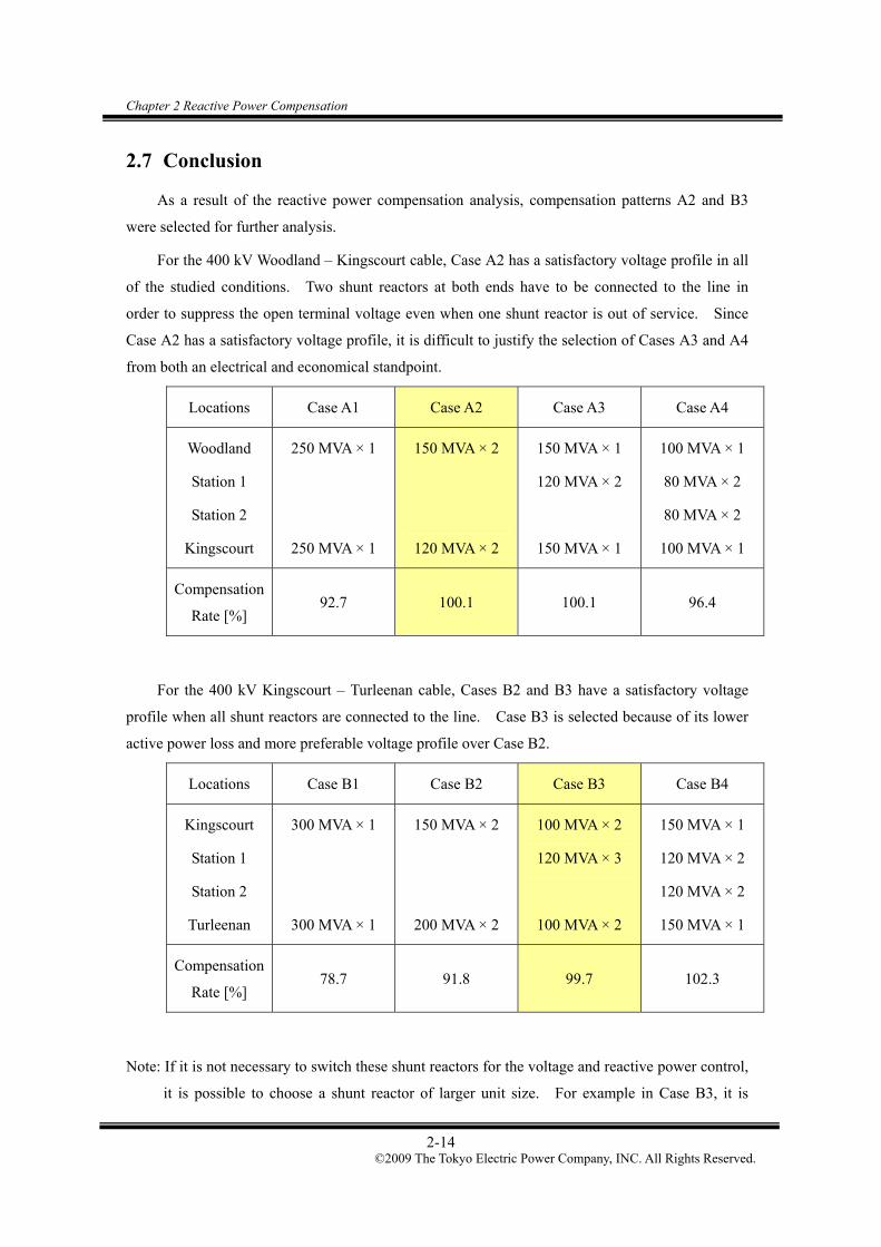
Chapter 2 Reactive Power Compensation
2-14 ©2009 The Tokyo Electric Power Company, INC. All Rights Reserved.
2.7 Conclusion
As a result of the reactive power compensation analysis, compensation patterns A2 and B3
were selected for further analysis.
For the 400 kV Woodland – Kingscourt cable, Case A2 has a satisfactory voltage profile in all
of the studied conditions. Two shunt reactors at both ends have to be connected to the line in
order to suppress the open terminal voltage even when one shunt reactor is out of service. Since
Case A2 has a satisfactory voltage profile, it is difficult to justify the selection of Cases A3 and A4
from both an electrical and economical standpoint.
Locations Case A1 Case A2 Case A3 Case A4
Woodland
Station 1
Station 2
Kingscourt
250 MVA × 1
250 MVA × 1
150 MVA × 2
120 MVA × 2
150 MVA × 1
120 MVA × 2
150 MVA × 1
100 MVA × 1
80 MVA × 2
80 MVA × 2
100 MVA × 1
Compensation
Rate [%] 92.7 100.1 100.1 96.4
For the 400 kV Kingscourt – Turleenan cable, Cases B2 and B3 have a satisfactory voltage
profile when all shunt reactors are connected to the line. Case B3 is selected because of its lower
active power loss and more preferable voltage profile over Case B2.
Locations Case B1 Case B2 Case B3 Case B4
Kingscourt
Station 1
Station 2
Turleenan
300 MVA × 1
300 MVA × 1
150 MVA × 2
200 MVA × 2
100 MVA × 2
120 MVA × 3
100 MVA × 2
150 MVA × 1
120 MVA × 2
120 MVA × 2
150 MVA × 1
Compensation
Rate [%] 78.7 91.8 99.7 102.3
Note: If it is not necessary to switch these shunt reactors for the voltage and reactive power control,
it is possible to choose a shunt reactor of larger unit size. For example in Case B3, it is

Chapter 2 Reactive Power Compensation
2-15 ©2009 The Tokyo Electric Power Company, INC. All Rights Reserved.
possible to install one unit of 200 MVA shunt reactor in Kingscourt instead of two units of
100 MVA. The compensation pattern in Case B3 was selected without the consideration of
the requirements for the voltage and reactive power control, since it is not included in the
scope of this study and the difference can have only small effects on the simulation results.
When a shunt reactor with large unit size is selected, an outage of this shunt reactor will
significantly lower the compensation rate of the cable line, which may limit the use of the
line during the outage.

Chapter 2 Reactive Power Compensation
2-16 ©2009 The Tokyo Electric Power Company, INC. All Rights Reserved.
2.8 Reactive Power Compensation for the Single Circuit Option
Charging capacity of the Woodland – Kingscourt – Turleenan line (Cu 2500 mm2 – 1 cct) is:
Woodland – Kingscourt: 699.2 MVA/cct @ 400 kV
Kingscourt – Turleenan: 988.6 MVA/cct @ 400 kV
Based on the maximum unit size found in the previous section, the following reactive power
compensation patterns were proposed:
Table 2-5 Proposed Compensation Patterns
Woodland – Kingscourt Kingscourt – Turleenan
Woodland
Station 1
Kingscourt
200 MVA × 2
150 MVA × 2
Kingscourt
Station 1
Kingscourt
150 MVA × 2
150 MVA × 2
150 MVA × 2
Compensation
Rate [%] 100.1
Compensation
Rate [%] 91.0
With the proposed compensation patterns, the voltage profile under the normal operating
conditions (no load and full load) is shown in Fig. 2.13. All the conditions were kept equal to the
previous studies in this section. The proposed compensation patterns yield preferable voltage
profiles under the normal operating conditions.
408
410
412
414
416
WO
OD
LA
ND T1
T2
T3
T4
T5
KIN
GSC
OU
RT T6
T7
T8
T9
T10
TU
RL
Vol
tage
[kV
]
No Load
Full Load
Fig. 2.13 Voltage profile in the normal operating condition.

Chapter 2 Reactive Power Compensation
2-17 ©2009 The Tokyo Electric Power Company, INC. All Rights Reserved.
To study the Ferranti phenomenon, the voltage profile when the Woodland terminal is opened
is shown in Fig. 2.14. When all shunt reactors (200 MVA × 2 units) are directly connected to the
line, the voltage along the line does not exceed 420 kV.
When one 200 MVA shunt reactor is connected to the bus or is not in service, the voltage near
the open terminal rises to 428 kV. The voltage rise from Kingscourt is, however, only 6 kV. The
open terminal voltage is kept below 420 kV as long as the Kingscourt 400 kV bus voltage is
maintained within 410 kV. It is not acceptable to connect all shunt reactors to the bus because the
open terminal voltage is too high.
410
420
430
440
450
WO
OD
LA
ND T1
T2
T3
T4
T5
KIN
GSC
OU
RT T6
T7
T8
T9
T10
TU
RL
400MVA
200MVA
No Reactor
Fig. 2.14 Voltage profile when the Woodland terminal is opened.
410
420
430
440
450
WO
OD
LA
ND T1
T2
T3
T4
T5
KIN
GSC
OU
RT T6
T7
T8
T9
T10
TU
RL
300MVA
150MVA
No Reactor
Fig. 2.15 Voltage profile when the Turleenan terminal is opened.

Chapter 2 Reactive Power Compensation
2-18 ©2009 The Tokyo Electric Power Company, INC. All Rights Reserved.
Finally, the voltage profile when the Turleenan terminal is opened is shown in Fig. 2.15.
When all shunt reactors (150 MVA × 2 units) are directly connected to the line, the voltage along
the line does not exceed 420 kV.
When one 150 MVA shunt reactor is connected to the bus or is not in service, the voltage near
the open terminal rises to 430 kV, and the voltage rise from Kingscourt is 10 kV. The open
terminal voltage is kept at 420 kV as long as the Kingscourt 400 kV bus voltage is maintained
within 410 kV. It is not acceptable to connect all shunt reactors to the bus because the open
terminal voltage is too high.
In conclusion, the proposed compensation patterns shown in Table 2-5 were considered
acceptable, and the shunt reactors have to be connected directly to the lines. The proposed
compensation patterns were used for further analysis.

Chapter 3 Model Setup
3-1 ©2009 The Tokyo Electric Power Company, INC. All Rights Reserved.
Chapter 3 Model Setup
3.1 Modeled Area for This Project
The entire 400 kV network is included in this model for the temporary overvoltage analysis
and the slow-front overvoltage analysis. The figure below shows an example of the model created
by ATP-Draw. Each component in the figure is explained in this section.
WDLD4LCC
125. km
MNPT4 OLDS4LCC
105. km
WMDL4
LCC
85. km
LAOI4LCC
85.23 km
DNST4LCC
44.77 km
Load
KELL4
LC
C
60.
km
SAT
Y Y
SAT
Y Y
SAT
Y Y
SAT
Y Y
SAT
Y Y
SAT
Y Y
110kV
400V
220kV
220kV
82km
KING4
TURL4
GR
OU
Pki
n-tu
r
WDLD2Y Y
I-Phi
Y Y
I-Phi
OLDS2
standard
YY
WMDL2
standard
YYLAOI2
standard
YY
59.3km
110kV
401.5L4.008
V
405.4L4.513
V
405.8L 5.1
V
GROUPturl tr
MNYPGSAT
Y Y
TRBT1SAT
Y Y
SAT
Y Y
standard
YY
standard
YY
BLLC2
DM136
SA
T
YY
50MVA
50MVATRBT4 LCC
6.5 km
KING2Y Y
I-Phi
FLAG4LCC
60. km
GROUPturl tr
KELL2
standard
YY
58km
GR
OU
Pw
dl-k
in
FLAG2
standard
YY
DNST2
standard
YYTRBT2
standard
YY
ABC 56.09km
216.9L 1.89V
123km
90km
20kmLOUT2
61km
18.43kmCORD2
17.83km
4.5kmHNST2
3.73km
1.4kmFING2
LOUTX
SAT
Y Y
SAT
Y Y
LOUTYSAT
Y Y
50km 50km
TAND2
19.94km
TURL2GROUP
turl tr
42km
5.63km
31.69km
26.04km
TAMN2
MAGF2
56.09km
0.2kmCAC2A
0.17kmCAC2B
COOL2
60km
OMAH2
25kmSTRB2
222.8L4.758
V
277.7L6.214
V
407.8L4.782
V
399.9L4.351
V
405.5L4.617V
404.2L3.001V
397.8L1.376V
400.2L0.863V
Load
Load
Load
Load
Load
Load
Load
Load
400V
17kV
110kV
82km
GR
OU
Pki
n-tu
r
58km
GR
OU
Pw
dl-k
in
GROUPreactor
22.5km
WDLD2
30.55kmMYNT2
80MVar
Reactor 80MVar
Fig. 3.1 Simulation model for the temporary overvoltage and slow-front overvoltage analysis.
Kingscourt – Turleenan line
Woodland – Kingscourt line

Chapter 3 Model Setup
3-2 ©2009 The Tokyo Electric Power Company, INC. All Rights Reserved.
3.2 Overhead Transmission Lines
400 kV overhead lines were modelled using a frequency dependent model (J. Marti model).
Input data for ATP-EMTP are shown in Table 3-1, and a cross-section diagram of transmission lines
and ground wires are shown in Fig. 3.2.
Table 3-1 Overhead Line Data
Types Inner
Radius [mm]
Outer Radius [mm]
Resistance per conductor [ohm/km]
Number of conductors in
a bundle
Separation between
conductors [cm]
Transmission Line (Curlew) 54/7
5.269 15.8 0.01655 2 45
Ground Wire 5.269 10 0.18 – –
Fig. 3.2 Cross-section diagram of transmission line (left) and ground wire (right).
The layout of transmission lines and ground wires were derived from the typical tower
configuration. The tower configuration (401 Configuration) applied to the existing 400 kV OHLs
is shown in Fig. 3.3. The layout of the existing 400 kV OHLs was derived from the figure as
shown in Table 3-2.
Table 3-2 Layout of the Existing 400 kV OHLs
Types Horizontal position [m] Vertical position [m]
-10.50 21.95
0 21.97 Conductors
+10.50 21.95
Ground wires -6.50, +6.50 32.00

Chapter 3 Model Setup
3-3 ©2009 The Tokyo Electric Power Company, INC. All Rights Reserved.
Fig. 3.3 Tower configuration of the existing 400 kV OHLs.

Chapter 3 Model Setup
3-4 ©2009 The Tokyo Electric Power Company, INC. All Rights Reserved.
The tower configuration (IVI Configuration) applied to the new 400 kV OHLs is shown in Fig.
3.4. The layout of the new 400 kV OHLs was derived from the figure as shown in Table 3-3.
Table 3-3 Layout of the New 400 kV OHLs
Types Horizontal position [m] Vertical position [m]
-9.50 21.70
0 27.75 Conductors
+9.50 21.70
Ground wires -6.75, +6.75 32.00

Chapter 3 Model Setup
3-5 ©2009 The Tokyo Electric Power Company, INC. All Rights Reserved.
Fig. 3.4 Tower configuration of the new 400 kV OHLs.

Chapter 3 Model Setup
3-6 ©2009 The Tokyo Electric Power Company, INC. All Rights Reserved.
3.3 Transformers
Model parameters of the Turleenan 400/275 kV transformer and the Kingscourt 400/220 kV
transformer were provided by NIE/EirGrid. These parameters are shown in Table 3-4. All
400/220 kV transformers in the RoI were assumed to have the same parameters as the Kingscourt
400/220 kV transformer.
Table 3-4 Model Parameters of 400 kV Transformers
For leakage inductances in Table 3-4, percent impedances were converted to mH by the
following calculations.
(x%1-2, x%1-3, x%2-3) → (x%1, x%2, x%3)
232%31%21%
1%
xxx
x
231%3221%
2%
xxx
x
221%32%31%
3%
xxx
x
(x%1, x%2, x%3) → (x1, x2, x3)
1000502
1
MVA100
)kV400(
100
21%
1
xx [mH]
1000502
1
MVA100
)220kVor 275(
100
22%
2
xx [mH]
1000502
1
MVA100
)21kVor 33(
100
23%
3
xx [mH]

Chapter 3 Model Setup
3-7 ©2009 The Tokyo Electric Power Company, INC. All Rights Reserved.
Internal resistance and leakage inductance of these transformers were obtained as follows:
Substations R1 [Ω] X1 [mH] R2 [Ω] X2 [mH] R3 [Ω] X3 [mH]
Turleenan 0.45981 104.91 0.25113 22.628 0.062879 8.2570
Kingscourt 0.3719 137.10 0.1793 0.001 0.035430 1.8812
Saturation characteristics of a 400/275/13 kV 750 MVA transformer in National Grid was
provided from NIE/EirGrid as shown in Table 3-5. The same saturation characteristics were
assumed for the Woodland and Kingscourt 400/220 kV transformer.
Table 3-5 Saturation Characteristic of the 400 kV Transformer (defined in tertiary)
I [A] Phi [Wb-T]
2.30940 51.63578
5.35781 55.07817
9.79186 58.52055
21.70836 61.96294
61.43004 65.40533
187.06140 68.84771
424.92960 72.29010
6267.24695 82.61725

Chapter 3 Model Setup
3-8 ©2009 The Tokyo Electric Power Company, INC. All Rights Reserved.
For transformer inrush studies, a magnetizing branch hysteresis curve was derived from the
saturation characteristic shown in Table 3-5 using the subroutine HYSDAT. The lower half of the
obtained hysteresis curve is shown in Table 3-6.
Table 3-6 Hysteresis Curve of the 400 kV Transformer (defined in primary)
I [A] Phi [Wb-T]
-29.4000 -1424.49
-3.6750 -1349.38
2.2050 -1243.19
5.1450 -966.929
9.9225 837.430
15.4350 1105.06
26.4600 1269.09
48.8775 1381.33
117.6000 1467.66
161.7000 1476.29
Another saturation characteristic as shown in Fig. 3.5 was also provided from NIE/EirGrid.
Fig. 3.5 Another saturation characteristic of the 400 kV transformers (defined in tertiary).

Chapter 3 Model Setup
3-9 ©2009 The Tokyo Electric Power Company, INC. All Rights Reserved.
From this saturation characteristic, another hysteresis curve was derived by HYSDAT as
shown in Table 3-7.
Table 3-7 Another Hysteresis Curve of the 400 kV Transformer (defined in primary)
I [A] Phi [Wb-T]
-0.65168 -1206.13
-0.081459 -1142.53
0.048876 -1052.62
0.11404 -818.707
0.21994 709.059
0.34213 935.665
0.58651 1074.55
1.0834 1169.58
2.6067 1242.68
3.5842 1249.99
This hysteresis characteristic was used only in one time domain simulation since it was
considered less severe compared to the one in Table 3-6.

Chapter 3 Model Setup
3-10 ©2009 The Tokyo Electric Power Company, INC. All Rights Reserved.
3.4 Shunt Reactors
Shunt reactors were connected to both ends of the 400 kV cables or 400 kV buses, in order to
compensate charging capacity of the cables. Only for the 400 kV Kingscourt – Turleenan line,
shunt reactors were also connected to the center of the line. Shunt reactors for the Woodland –
Kingscourt – Turleenan line were modeled based on the results of the analysis in Chapter 1. 400
kV shunt reactors in the simulation model are shown in Table 3-8.
Table 3-8 400 kV Shunt Reactors in the Simulation Model
Woodland – Kingscourt (58 km) Woodland: 150 MVA × 2
Kingscourt: 120 MVA × 2
Kingscourt – Turleenan (82 km)
Kingscourt: 100 MVA × 2
Centre: 120 MVA × 3
Turleenan: 100 MVA × 2
Woodland – Oldstreet (125 km) Woodland: 80 MVA × 1
Moneypoint – Tarbert (6.5 km) Moneypoint: 50 MVA × 1
Tarbert: 50 MVA × 1
When 400 kV shunt reactors are close to the point of interest, they are modeled with the
saturation characteristic. Otherwise, they are modeled as linear inductances.

Chapter 3 Model Setup
3-11 ©2009 The Tokyo Electric Power Company, INC. All Rights Reserved.
Note: Other sections of this chapter have been deleted.

Chapter 4 Temporary Overvoltage Analysis
4-1 ©2009 The Tokyo Electric Power Company, INC. All Rights Reserved.
Chapter 4 Temporary Overvoltage Analysis
For long EHV cables, temporary overvoltages are of highest concerns in terms of the safe
operation after the installation. Highest temporary overvoltages are often higher than highest
slow-front overvoltages.
Due to the large capacitance associated with the long EHV cable and the inductance of shunt
reactors for the reactive power compensation, the following temporary overvoltages require a close
attention for the network with long EHV cables. The theoretical backgrounds relating the large
capacitance and the inductance to these temporary overvoltages are given in the beginning of each
section:
(1) Parallel resonance overvoltage
(2) Oscillatory overvoltage caused by the system islanding
For equipment whose highest voltage is higher than 245 kV, the standard short-duration
power-frequency withstand voltage is not specified in IEC, but it is specified by a utility or a
manufacturer. Surge arresters are generally the weakest among different equipment. The
temporary overvoltages have to be evaluated against typical withstand voltage and energy
absorption capability of surge arresters. Note that the temporary overvoltages may be evaluated
with SIWV depending on their decay time.

Chapter 4 Temporary Overvoltage Analysis
4-2 ©2009 The Tokyo Electric Power Company, INC. All Rights Reserved.
4.1 Parallel Resonance Overvoltage
4.1.1 Overview
In EHV systems, the highest concern in terms of parallel resonance is the second harmonic
current injection due to transformer inrush. Parallel resonance frequencies were found from the
results of frequency scan in EMTP.
It is necessary to consider different operating configurations since it affects parallel resonance
frequencies. In order to find the most critical parallel resonance condition, a number of on/off
combinations of the 400 kV lines and shunt reactors were studied as shown in blue in Fig. 4.1.
When the EHV underground cable has significant length, the switching overvoltage caused by
its energisation can have very low frequency components for switching overvoltage. For example,
energisation of the EHV underground cable of the length of around 100 km may largely contain
third to fifth harmonics. Therefore, parallel resonance frequencies higher than 100 Hz (second
harmonic) must be searched in frequency scan.
Turleenan Kingscourt WoodlandMNYPGCoolkeeragh
Omagh
Flagford
A AC C
D D
E E
B B
Parallel resonance frequency seen from the Woodland substation
Parallel resonance frequency seen from the Kingscourt substation
Closed switch
Connected 400kV shunt reactor
Combinational On/Off switch
Combinational On/Off 400kV shunt reactor

Chapter 4 Temporary Overvoltage Analysis
4-3 ©2009 The Tokyo Electric Power Company, INC. All Rights Reserved.
Parallel resonance frequency seen from the Turleenan substation
Fig. 4.1 Frequency sweep for the parallel resonance overvoltage analysis.
After the frequency scan, a time domain simulation under the most critical conditions was
performed. If parallel resonance frequency seen from the 400 kV Woodland bus is assumed to be
the severest condition with an outage of the Kingscourt – Turleenan lines, the Woodland 400/220
kV transformer energisation is studied as shown in Fig. 4.2.
Fig. 4.2 Sample scenario of the time domain simulation for the parallel resonance overvoltage
analysis.
Close
Open
On
Closed switch
Connected 400kV shunt reactor
Combinational On/Off switch
Combinational On/Off 400kV shunt reactor

Chapter 4 Temporary Overvoltage Analysis
4-4 ©2009 The Tokyo Electric Power Company, INC. All Rights Reserved.
4.1.2 Fault Current Level
In the parallel resonance analysis, an effect of the fault current level (source impedance) at
Woodland 220 kV, Kingscourt 220 kV, and Turleenan 275 kV buses was studied as one of the
parameters. First, the fault current calculation was performed at these buses to find a reasonable
range for this parameter. Here, power flow data for the planned transmission system in 2020 were
used for the calculation.
The results of the calculation are shown in Table 4-1. Since it is necessary to find the fault
current level in the 275 and 220 kV network, fault current that flows from the 400 kV network is
not included in the calculation result. In the table, values of source impedance that correspond to
the fault current levels are shown in parentheses.
Table 4-1 Fault Current Levels at Woodland, Kingscourt, and Turleenan LV Side Buses
Summer off-peak
Winter peak with
maximum wind Normal winter peak
Woodland 220 kV 8.673 kA
(46.62 mH)
11.24 kA
(35.97 mH)
14.59 kA
(27.71 mH)
Kingscourt 220 kV 7.657 kA
(52.80 mH)
8.623 kA
(46.89 mH)
8.679 kA
(46.58 mH)
Turleenan 275 kV 13.43 kA
(37.62 mH)
18.91 kA
(26.73 mH)
15.99 kA
(31.60 mH)
Generators included in the simulation model are fewer than those in service in summer
off-peak power flow data. The generators included in the simulation model caused the following
fault current levels at Woodland, Kingscourt, and Turleenan LV side buses.
Table 4-2 Fault Current Levels at Woodland, Kingscourt, and Turleenan LV Side Buses
Summer off-peak
Woodland 220 kV 1.543 kA
(262.0 mH)
Kingscourt 220 kV 1.671 kA
(241.9 mH)
Turleenan 275 kV 1.257 kA
(402.0 mH)

Chapter 4 Temporary Overvoltage Analysis
4-5 ©2009 The Tokyo Electric Power Company, INC. All Rights Reserved.
An adjustment of the fault current level can be achieved by adding a dummy source at
Woodland, Kingscourt, and Turleenan LV side buses with different source impedances. Based on
current calculation results of the fault, the source impedance values were varied in the range shown
below, considering the difference between the values in Table 4-1 and the values in Table 4-2.
Table 4-3 Assumed Range of Source Impedance Values
Woodland 220 kV 20 – 60 mH
Kingscourt 220 kV 40 – 60 mH
Turleenan 275 kV 20 – 50 mH

Chapter 4 Temporary Overvoltage Analysis
4-6 ©2009 The Tokyo Electric Power Company, INC. All Rights Reserved.
4.1.3 Study of the Simple Network
In this section, the characteristic of the 400 kV Woodland – Kingscourt – Turleenan line with a
generator was studied. As a simple network model, only one voltage source is assumed at
Turleenan behind source impedance. With the existence of this voltage source, parallel resonance
frequency shifts from LC
f2
1 to
CLLCf
0
11
2
1
(L0: source impedance).
In this simple theoretical calculation, the source impedance necessary to shift parallel
resonance frequency from 50.0 Hz to 100 Hz is
1001080.51
1
1080.511959.0
1
2
16
06
L
mH 2.650 L
The effect of source impedance was then confirmed by frequency scan. Fig. 4.3 shows the
simulation model for frequency scan. Source impedance of 65.2 mH is connected to the
Turleenan 400 kV bus.
1A
V
82km
KING4 TURL4GROUPkin-tur
58km
WDLD4GROUPwdl-kin
82km
GROUPkin-tur
58km
GROUPwdl-kin
65.2mH
Fig. 4.3 Simulation model for frequency scan to study the simple network.
The results of frequency scan are shown in Fig. 4.4. Parallel resonance frequency was
shifted from 48.3 Hz to around 90.0 Hz. It can be seen from the figure that source impedance has
a small effect on the frequency response at higher frequencies. This is reasonable since the
magnitude of source impedance (inductance) becomes larger at higher frequencies.
In Fig. 4.4, a frequency scan was performed with a large frequency step (10 Hz). In order to
find an effect of source impedance on the magnitude of impedance at parallel resonance, frequency
scan must be performed using a smaller frequency step.

Chapter 4 Temporary Overvoltage Analysis
4-7 ©2009 The Tokyo Electric Power Company, INC. All Rights Reserved.
cableonly.pl4: v:WDLD4A cableonly_65.2mh.pl4: v:WDLD4A
0 1000 2000 3000 4000 5000[s]0
300
600
900
1200
1500
[V]
Fig. 4.4 Characteristic of the simple network.
Fig. 4.5 shows the result of a frequency scan with different source impedance values of 1000,
100, and 65.2 mH. Here, the frequency scan was performed only near the highest peak with a
small frequency step (0.1 Hz). The vertical axis of the figure is the log scale. It can be seen that
the magnitude of impedance at parallel resonance significantly decreases for smaller source
impedance, that is for a higher fault current level.
100
1000
10000
100000
40 50 60 70 80 90 100[Hz]
[Ω]
No Source
1000 mH
100 mH
65.2 mH
Fig. 4.5 Effect of source impedance on the characteristic of the simple network.
with source impedance
without source impedance
Smaller source impedance

Chapter 4 Temporary Overvoltage Analysis
4-8 ©2009 The Tokyo Electric Power Company, INC. All Rights Reserved.
An outage of the shunt reactor is not assumed to have a large impact on parallel resonance,
also in this simulation model with a generator. In contrast, it can be understood that an outage of a
400 kV cable has some effect on parallel resonance in this simple network. It can be seen from
the theoretical equation CLLC
f0
11
2
1
that an outage of a 400 kV cable (change of C) will
change the effect of source impedance.
First, an outage of the largest shunt reactor (150 MVA) was studied by a frequency scan as
shown in Fig. 4.6. The source impedance was fixed to 100 mH. An outage of the largest shunt
reactor shifted the parallel resonance frequency only by 0.9 Hz, as was expected based on the
theoretical equation. In addition, the magnitude of impedance at parallel resonance was not
changed by the shunt reactor outage.
cableonly_100mh_zoom.pl4: v:WDLD4A cableonly_100mh_shroutage_zoom.pl4: v:WDLD4A
75 77 79 81 83 85[Hz]0
900
1800
2700
3600
4500
[Ω]
Fig. 4.6 Effect of a shunt reactor outage on the characteristic of the simple network.
Fig. 4.7 shows the effect of a 400 kV cable outage. An outage of one circuit of the
Kingscourt – Turleenan lines caused parallel resonance frequency to shift by 4.4 Hz. In addition,
the magnitude of impedance at parallel resonance was lowered from 3987 Ω to 2238 Ω.
78.1 Hz 79.0 Hz
one reactor outage
all reactors in service

Chapter 4 Temporary Overvoltage Analysis
4-9 ©2009 The Tokyo Electric Power Company, INC. All Rights Reserved.
cableonly_100mh_zoom.pl4: v:WDLD4A cableonly_100mh_kctloutage_zoom.pl4: v:WDLD4A
75 78 81 84 87 90[Hz]0
500
1000
1500
2000
2500
3000
3500
4000
[Ω]
Fig. 4.7 Effect of a line outage on the characteristic of the simple network.
Then, an effect of target frequency of the Bergeron model was studied. Target frequency of
all cable models were changed from 50 Hz to 100 Hz.
cableonly_100mh_zoom.pl4: v:WDLD4A cableonly_100mh_zoom_target100hz.pl4: v:WDLD4A
75 77 79 81 83 85[Hz]0
500
1000
1500
2000
2500
3000
3500
4000
[Ω]
Fig. 4.8 Effect of a line outage on the characteristic of the simple network.
79.0 Hz
one line outage
all lines in service
83.4 Hz
target frequency 100 Hz
target frequency 50 Hz
79.0 Hz 79.7 Hz

Chapter 4 Temporary Overvoltage Analysis
4-10 ©2009 The Tokyo Electric Power Company, INC. All Rights Reserved.
Fig. 4.8 shows the result of the frequency scan. Parallel resonance frequency was shifted
only by 0.7 Hz by changing target frequency from 50 Hz to 100 Hz. The target frequency was set
to 50 Hz for further analysis since the magnitude of impedance at parallel resonance frequency was
larger when the target frequency was set to 50 Hz.
In conclusion, the effects of the parameters have been summarized in Table 4-4. Since the
shunt reactor outage does not have a significant impact on parallel resonance frequency, it has to be
adjusted by changing the fault current level or through line outages. Additionally, in order to yield
a severe condition, some OHL outages should be considered in order to increase the magnitude of
impedance at parallel resonance frequency.
Note that the result summarized in this table applies only to this study, since these effects
depend on the compensation rate, the unit size of shunt reactor, and so on.
Table 4-4 Effect of a Shunt Reactor / Line Outage and Fault Current Level (Summary)
Parallel resonance frequency Magnitude of impedance
Target frequency Very small Moderate
Shunt reactor outage Very small No effect
Line outage Moderate Moderate
Fault current level Large Very large

Chapter 4 Temporary Overvoltage Analysis
4-11 ©2009 The Tokyo Electric Power Company, INC. All Rights Reserved.
4.1.4 Transformer Inrush Current
In this section, transformer energisation was studied in order to find the frequency components
contained in transformer inrush current. First, energisation of the 400/220 kV Woodland
transformer was simulated. Fig. 4.9 shows inrush current into the transformer. The switch
timing was selected so that the largest inrush current appeared in Phase A. Residual flux in Phases
A and B were set to 85 % of the rated flux.
(file Inrush_Woodland_Imp50mH.pl4; x-var t) c:WDLD4A-WL_TRA c:WDLD4B-WL_TRB c:WDLD4C-WL_TRC 0.00 0.04 0.08 0.12 0.16 0.20[s]
-4000
-2000
0
2000
4000
6000
[A]
Fig. 4.9 Inrush current into the 400/220 Woodland transformer.
Inrush current largely contains second harmonic. As shown in Fig. 4.10, Fourier transform
of inrush current (Phase A) shows that second harmonic current 513.2 A is contained in inrush
current.
0 5 10 15 20 25 300
500
1000
1500
2000
2500
3000[A]
harmonic order
Fig. 4.10 Fourier transform of inrush current.
Second harmonic: 513.2A

Chapter 4 Temporary Overvoltage Analysis
4-12 ©2009 The Tokyo Electric Power Company, INC. All Rights Reserved.
Fig. 4.11 shows the result of Fourier transform when it was performed with a frequency
resolution of 1 Hz.
0 30 60 90 120 1500
400
800
1200
1600
2000
[A]
Fig. 4.11 Fourier transform of inrush current (1 Hz step).
It is known that inrush current reaches its maximum if a transformer is energised when the bus
voltage crosses the zero point. In contrast, second harmonic contained in inrush current reaches
its maximum at the different switch timing, which has to be found by simulations. As a result of
the simulations shown in Fig. 4.12, it was determined that transformer energisation was simulated
at switch timings between 10 ms and 14 ms by 1 ms step.
0
500
1000
1500
2000
2500
3000
0 0.005 0.01 0.015 0.02
Switch timing [s]
Inru
sh c
urre
nt [
A]
Fundamental
Second harmonic
Fig. 4.12 Fundamental component and second harmonic contained in inrush current.
Second harmonic: 678.0A
[Hz]

Chapter 4 Temporary Overvoltage Analysis
4-13 ©2009 The Tokyo Electric Power Company, INC. All Rights Reserved.
4.1.5 Parallel Resonance Frequency Seen from Woodland 400 kV
Parallel resonance frequency of the network seen from Woodland 400 kV was found by
frequency scan using the simulation model in Fig. 4.13.
LCC
125. km
MNPT4 OLDS4LCC
105. km
WMDL4
LCC
85. km
LAOI4LCC
85.23 km
DNST4LCC
44.77 km
Load
KELL4
LCC
60.
km
SAT
Y Y
SAT
Y Y
SAT
Y Y
SAT
Y Y
SAT
Y Y
SAT
Y Y
82km
KING4
TURL4
GR
OU
Pki
n-tu
r
WDLD4 WDLD2Y Y
I-Phi
Y Y
I-Phi
OLDS2
standard
YY
WMDL2
standard
YYLAOI2
standard
YY
59.3km
0.055L-164.
V
0.014L 164.
V
0.005L3.529
V
GROUPturl tr
MNYPGSAT
Y Y
TRBT1SAT
Y Y
SAT
Y Y
standard
YY
standard
YY
BLLC2
DM136
SA
T
YY
50MVA
50MVATRBT4
KING2Y Y
I-Phi
FLAG4LCC
60. km
GROUPturl tr
KELL2
standard
YY
58km
GR
OU
Pw
dl-k
in
FLAG2
standard
YY
DNST2
standard
YYTRBT2
standard
YY
ABC 56.09km
0.001L150.6V
123km
90km
20kmLOUT2
61km
18.43kmCORD2
17.83km
4.5kmHNST2
3.73km
1.4kmFING2
LOUTX
SAT
Y Y
SAT
Y Y
LOUTYSAT
Y Y
50km 50km
TAND2
19.94km
TURL2GROUP
turl tr
42km
5.63km
31.69km
26.04km
TAMN2
MAGF2
56.09km
0.2kmCAC2A
0.17kmCAC2B
COOL2
60km
OMAH2
25kmSTRB2
0.01L149.4
V
0.028L-171.
V
0.136L-3.39
V
0.004L-13.9
V
0.01L28.81V
1A
0.05L146.3V
Load
Load
Load
Load
Load
Load
Load
Load
82km
GR
OU
Pki
n-tu
r
58km
GR
OU
Pw
dl-k
in
GROUPreactor
22.5km
WDLD2
30.55kmMYNT2
6.5km
GROUPmp-tb
GROUPmp-tb
60mH
60mH
50mH
80MVar
Reactor 80MVar
Dummy source
Dummy source
Dummy source
Fig. 4.13 Simulation model for frequency scan seen from Woodland 400 kV.
Current source (1 Amp)
Kingscourt – Turleenan line
Woodland – Kingscourt line

Chapter 4 Temporary Overvoltage Analysis
4-14 ©2009 The Tokyo Electric Power Company, INC. All Rights Reserved.
In the first example, the largest source impedance (lowest fault current level) in Table 4-3 was
set to the Woodland 220 kV, the Kingscourt 220 kV, and the Turleenan 275 kV buses. The result
of the frequency scan is shown in Fig. 4.14. The highest peak was found at 90 Hz, and other high
peaks were not a level requiring careful consideration.
(file woodland_wide.pl4; x-var t) v:WDLD4A v:WDLD4B v:WDLD4C 0 1000 2000 3000 4000 5000 6000[Hz]
0
100
200
300
400
500
600
[Ω]
Fig. 4.14 Parallel resonance frequency of the network seen from Woodland 400 kV.
As a result, an energisation of the Woodland 400/220 kV transformer was considered as the
most severe source of harmonic current injection. Since parallel resonance frequency was found
to be 90 Hz, it was necessary to shift it by 10 Hz.
90Hz

Chapter 4 Temporary Overvoltage Analysis
4-15 ©2009 The Tokyo Electric Power Company, INC. All Rights Reserved.
Next, in order to realize a higher magnitude of impedance at parallel resonance, some
combinations of OHL outages were studied. The result of the analysis is shown in Fig. 4.15. As
a result of the analysis, two 400 kV OHLs, Woodland – Oldstreet line and Kingscourt – Flagford
line, will be considered as out of service, in order to achieve a higher magnitude of impedance.
woodland.pl4: v:WDLD4A woodland_wlosoutage.pl4: v:WDLD4A woodland_kcffoutage.pl4: v:WDLD4A woodland_wlosoutage_kcffoutage.pl4: v:WDLD4A
0 300 600 900 1200 1500[Hz]0
200
400
600
800
1000
1200
[Ω]
Fig. 4.15 Effect of OHL outages on parallel resonance frequency.
all OHLs in service
Woodland-Oldstreet line outage
Kingscourt-Flagford line outage
both two OHLs outage
60 70 80 90 100 110 120[Hz]0
200
400
600
800
1000
1200
[Ω]
Zoom

Chapter 4 Temporary Overvoltage Analysis
4-16 ©2009 The Tokyo Electric Power Company, INC. All Rights Reserved.
Considering the operating status of the Woodland – Kingscourt – Turleenan line, the four cases
shown in Table 4-5 were studied. For each case, source impedance at the Turleenan 275 kV bus
was adjusted in order to yield parallel resonance frequency of 100 Hz. The value of this source
impedance and the magnitude of impedance at parallel resonance frequency are shown in Table 4-5.
Table 4-5 Magnitude of impedance at parallel resonance frequency (Woodland)
Woodland –
Kingscourt line
Kingscourt –
Turleenan line
Source impedance
(Turleenan)
Magnitude of
impedance
Case 1 Two circuits Two circuits 17.0 mH 1642 Ω
Case 2 Two circuits One circuit 51.0 mH 1326 Ω
Case 3 One circuit Two circuits 39.8 mH 1142 Ω
Case 4 One circuit One circuit 252.0 mH 856 Ω
The reasonable range of source impedance values at Turleenan 275 kV was 20 – 50 mH.
However, in order to shift parallel resonance frequency to 100 Hz in Case 4, it was necessary to set
the values of source impedance at Turleenan 275 kV bus much higher than this range.
Finally, a time domain simulation was carried out under the assumed severest conditions, Case
1. As stated in the previous section, transformer energisation was simulated at switch timings
between 10 ms and 14 ms in 1 ms steps in order to find the severest switch timing. The result of
the analysis is summarized in Table 4-6.
Table 4-6 Highest Overvoltage for Different Switch Timings
Highest overvoltage [kV] Switch timing
[ms] Phase A Phase B Phase C
10 509.8 444.4 528.5
11 484.0 465.4 532.7
12 445.1 489.8 540.7
13 420.6 509.3 534.5
14 418.0 511.4 532.9

Chapter 4 Temporary Overvoltage Analysis
4-17 ©2009 The Tokyo Electric Power Company, INC. All Rights Reserved.
As can be seen from Table 4-6, the highest overvoltage always occurred in Phase C, and it is
not very sensitive to the switch timing. When the switch timing is changed from 12 ms to 14 ms,
the change in the overvoltage is only 7.8 kV. The voltage of the Woodland 400 kV bus and inrush
current into the Woodland 400/220 kV transformer for the switch timing 12 ms are shown in Fig.
4.16 and Fig. 4.17.
(file inrush_woodland_case1_12ms.pl4; x-var t) v:WDLD4A v:WDLD4B v:WDLD4C 0.0 0.2 0.4 0.6 0.8 1.0[s]
-500
-280
-60
160
380
600
[kV]
Fig. 4.16 Woodland 400 kV bus voltage in transformer inrush.
(file inrush_woodland_case1_12ms.pl4; x-var t) c:WDLD4A-WL_TRA c:WDLD4B-WL_TRB c:WDLD4C-WL_TRC 0.0 0.2 0.4 0.6 0.8 1.0[s]
-5000
-3750
-2500
-1250
0
1250
2500
3750
5000
[A]
Fig. 4.17 Inrush current into the Woodland 400/220 kV transformer.
540.7kV (1.66 pu)
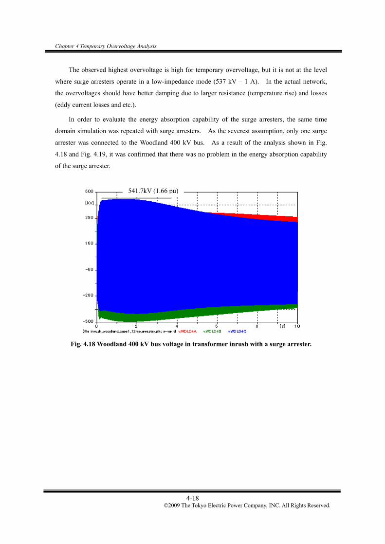
Chapter 4 Temporary Overvoltage Analysis
4-18 ©2009 The Tokyo Electric Power Company, INC. All Rights Reserved.
The observed highest overvoltage is high for temporary overvoltage, but it is not at the level
where surge arresters operate in a low-impedance mode (537 kV – 1 A). In the actual network,
the overvoltages should have better damping due to larger resistance (temperature rise) and losses
(eddy current losses and etc.).
In order to evaluate the energy absorption capability of the surge arresters, the same time
domain simulation was repeated with surge arresters. As the severest assumption, only one surge
arrester was connected to the Woodland 400 kV bus. As a result of the analysis shown in Fig.
4.18 and Fig. 4.19, it was confirmed that there was no problem in the energy absorption capability
of the surge arrester.
Fig. 4.18 Woodland 400 kV bus voltage in transformer inrush with a surge arrester.
541.7kV (1.66 pu)

Chapter 4 Temporary Overvoltage Analysis
4-19 ©2009 The Tokyo Electric Power Company, INC. All Rights Reserved.
Fig. 4.19 Energy absorbed by the surge arrester.
The withstand voltages of surge arresters are often given in their specification. For example,
Siemens 3ES5 336-5PM51-1HA2-Z has the withstand voltages as shown in Table 4-7. As can be
seen from the table, the observed highest overvoltage 541.7 kV (1.66 pu, peak) was higher than the
temporary overvoltage allowed for 10 seconds.
Table 4-7 Withstand Voltages of Surge Arresters (r.m.s.)
Maximum continuous operating voltage 269 kV (1.16 pu)
Power frequency withstand voltage (1 min) 364 kV (1.58 pu)
10 s 370 kV (1.60 pu) Temporary overvoltage
1 s 390 kV (1.69 pu)
From a manufacturer’s standpoint, it is possible to develop a surge arrester with higher
withstand voltages, for example 1.8 pu for 10 seconds. With this in mind, the observed
overvoltage is not at the level which affects the feasibility of the 400 kV Woodland – Kingscourt –
Turleenan line.
It may, however, lead to higher protective levels ensured by the arrester, which may affect the
insulation design of other equipment. These additional costs need to be evaluated by the
manufacturer. Finally, it will of course affect the total insulation coordination studied by utilities.

Chapter 4 Temporary Overvoltage Analysis
4-20 ©2009 The Tokyo Electric Power Company, INC. All Rights Reserved.
The time domain simulations as shown in Fig. 4.16 – Fig. 4.19 were performed with the
hysteresis curve in Table 3-6, which was derived from the saturation characteristics of the
400/275/13 kV 750 MVA transformer in the National Grid. Here, the time domain simulation was
repeated with the other hysteresis curve as shown in Table 3-7. The Woodland 400/220 kV
transformer was energised at 12 ms.
The waveform of the inrush current is shown in Fig. 4.20. Due to the difference between the
two hysteresis curves, the magnitude of inrush current is significantly lower compared to the one in
Fig. 4.17.
(file Inrush_Woodland_Case1_12ms_EirGridHysteresis.pl4; x-var t) c:WDLD4A-WL_TRA c:WDLD4B-WL_TRB c:WDLD4C-WL_TRC
0.0 0.2 0.4 0.6 0.8 1.0[s]-300
-200
-100
0
100
200
300
[A]
Fig. 4.20 Inrush current into the Woodland 400/220 kV transformer with the other hysteresis
curve.

Chapter 4 Temporary Overvoltage Analysis
4-21 ©2009 The Tokyo Electric Power Company, INC. All Rights Reserved.
The voltage of the Woodland 400 kV bus is shown in Fig. 4.21. The highest voltage of 337.8
kV (1.03 pu) was observed in Phase A. Since inrush current is small, an overvoltage caused by
parallel resonance was not observed.
(file Inrush_Woodland_Case1_12ms_EirGridHysteresis.pl4; x-var t) v:WDLD4A v:WDLD4B v:WDLD4C 0.0 0.2 0.4 0.6 0.8 1.0[s]
-400
-300
-200
-100
0
100
200
300
400
[kV]
Fig. 4.21 Woodland 400 kV bus voltage in transformer inrush with the other hysteresis curve.
Considering this result, the transformer inrush studies were hereafter performed only with the
hysteresis curve derived from the 400/275/13 kV 750 MVA transformer data in the National Grid.
337.8kV

Chapter 4 Temporary Overvoltage Analysis
4-22 ©2009 The Tokyo Electric Power Company, INC. All Rights Reserved.
4.1.6 Parallel Resonance Frequency Seen from Kingscourt 400 kV
In this section, parallel resonance frequency seen from the Kingscourt 400 kV bus was studied.
First, the result of the frequency scan is shown in Fig. 4.22. For the analysis, the largest source
impedance (lowest fault current level) in Table 4-3 was set to Woodland 220 kV, Kingscourt 220 kV,
and Turleenan 275 kV buses. As in the frequency scan result seen from Kingscourt 400 kV, the
highest peak was found at 90 Hz, and other high peaks were not at a level needing careful
consideration.
(file kingscourt_wide.pl4; x-var t) v:KING4A v:KING4B v:KING4C 0 1000 2000 3000 4000 5000 6000[Hz]
0
100
200
300
400
500
600
700
[Ω]
Fig. 4.22 Parallel resonance frequency of the network seen from Kingscourt 400 kV.
As a result, an energisation of the Kingscourt 400/220 kV transformer was considered as the
severest source of harmonic current injection. Since parallel resonance frequency was found to be
at 90 Hz, it was necessary to shift it by 10 Hz.
90Hz

Chapter 4 Temporary Overvoltage Analysis
4-23 ©2009 The Tokyo Electric Power Company, INC. All Rights Reserved.
The same four combinations were studied with regard to the operating status of the 400 kV
Woodland – Kingscourt – Turleenan line, as shown in Table 4-8. As in the previous section,
outages of the Woodland – Oldstreet line and the Kingscourt – Flagford line were assumed in order
to have larger impedance at parallel resonance frequency, without shifting the parallel resonance
frequency.
For each case, the source impedance at Turleenan 275 kV bus was adjusted first in order to
yield a parallel resonance frequency at 100 Hz. Source impedance at Woodland 220 kV bus was
also adjusted when it was not possible to shift parallel resonance frequency to 100 Hz by only
adjusting the source impedance at the Turleenan 275 kV bus. The values of these source
impedances and the magnitude of impedance at parallel resonance frequency are shown in Table
4-8.
Table 4-8 Magnitude of impedance at parallel resonance frequency (Kingscourt)
Source impedance Woodland –
Kingscourt line
Kingscourt –
Turleenan lineTurleenan Woodland
Magnitude of
impedance
Case 1 Two circuits Two circuits 20.0 mH 24.8 mH 2606 Ω
Case 2 Two circuits One circuit 31.3 mH 60.0 mH 1263 Ω
Case 3 One circuit Two circuits 27.0 mH 60.0 mH 1247 Ω
Case 4 One circuit One circuit 130.0 mH 60.0 mH 923 Ω
The reasonable range of source impedance value at Turleenan 275 kV was 20 – 50 mH.
However, in order to shift parallel resonance frequency to 100 Hz in Case 4, it was necessary to set
the value of source impedance at Turleenan 275 kV bus much higher than this range.
Finally, the time domain simulation was carried out under the assumed severest conditions,
Case 1. The voltage of the Kingscourt 400 kV bus and inrush current into the Woodland 400/220
kV transformer are shown in Fig. 4.23 and Fig. 4.24. Since it was discovered that the switch
timing does not have a large effect on the overvoltage, the transformer was energised at voltage
zero. As a result, the highest voltage observed at the Kingscourt 400 kV bus was 515.8 kV (1.58
pu) in Phase C. This is high for a temporary overvoltage, but is not at the level where surge
arresters operate in a low-impedance mode (511 kV – 0.01 A). This is not a concern for the
operation of the 400 kV Woodland – Kingscourt – Turleenan line.

Chapter 4 Temporary Overvoltage Analysis
4-24 ©2009 The Tokyo Electric Power Company, INC. All Rights Reserved.
(file inrush_kingscourt_case1_10s.pl4; x-var t) v:KING4A v:KING4B v:KING4C 0 2 4 6 8 10[s]
-600
-400
-200
0
200
400
600
[kV]
(file inrush_kingscourt_case1_1s.pl4; x-var t) v:KING4A v:KING4B v:KING4C 0.0 0.2 0.4 0.6 0.8 1.0[s]
-600
-400
-200
0
200
400
600
[kV]
Fig. 4.23 Kingscourt 400 kV bus voltage in transformer inrush.
501.2kV
515.8kV Zoom

Chapter 4 Temporary Overvoltage Analysis
4-25 ©2009 The Tokyo Electric Power Company, INC. All Rights Reserved.
(file inrush_kingscourt_case1_1s.pl4; x-var t) c:KING4A-KC_TRA c:KING4B-KC_TRB c:KING4C-KC_TRC 0.0 0.2 0.4 0.6 0.8 1.0[s]
-4000
-2000
0
2000
4000
6000
[A]
Fig. 4.24 Inrush current into the Kingscourt 400/220 kV transformer.

Chapter 4 Temporary Overvoltage Analysis
4-26 ©2009 The Tokyo Electric Power Company, INC. All Rights Reserved.
4.1.7 Parallel Resonance Frequency Seen from Turleenan 400 kV
In this section, parallel resonance frequency seen from the Turleenan 400 kV bus was studied.
First, the result of frequency scan is shown in Fig. 4.25. For the analysis, the largest source
impedance (lowest fault current level) in Table 4-3 was set to Woodland 220 kV, Kingscourt 220 kV,
and Turleenan 275 kV buses. As in the frequency scan result seen from Turleenan 400 kV, the
highest peak was found at 90 Hz, and other high peaks were not at a level requiring careful
consideration.
(file turleenan_wide.pl4; x-var t) v:TURL4A v:TURL4B v:TURL4C 0 1000 2000 3000 4000 5000 6000[Hz]
0
100
200
300
400
500
[Ω]
Fig. 4.25 Parallel resonance frequency of the network seen from Turleenan 400 kV.
As a result, an energisation of the Turleenan 400/275 kV transformer was considered as the
severest source of harmonic current injection. Since parallel resonance frequency was found to be
90 Hz, it was necessary to shift it by 10 Hz.
90Hz

Chapter 4 Temporary Overvoltage Analysis
4-27 ©2009 The Tokyo Electric Power Company, INC. All Rights Reserved.
The same four combinations were studied with regard to the operating status of the 400 kV
Woodland – Kingscourt – Turleenan line, as shown in Table 4-9. As in the previous sections,
outages of the Woodland – Oldstreet line and the Kingscourt – Flagford line were assumed in order
to have larger impedance at parallel resonance frequency, without shifting parallel resonance
frequency.
For each case, the source impedance at Woodland 220 kV bus was adjusted first in order to
yield a parallel resonance frequency at 100 Hz. Source impedance at Kingscourt 220 kV bus was
also adjusted when it was not possible to shift parallel resonance frequency to 100 Hz by only
adjusting the source impedance at the Woodland 220 kV bus. The values of these source
impedances and the magnitude of impedance at parallel resonance frequency are shown in Table
4-9.
Table 4-9 Magnitude of impedance at parallel resonance frequency (Turleenan)
Source impedance Woodland –
Kingscourt line
Kingscourt –
Turleenan lineWoodland Kingscourt
Magnitude of
impedance
Case 1 Two circuits Two circuits 20.0 mH 31.0 mH 1711 Ω
Case 2 Two circuits One circuit 70.0 mH 60.0 mH 598 Ω
Case 3 One circuit Two circuits 39.0 mH 60.0 mH 1230 Ω
Case 4 One circuit One circuit 250.0 mH 250.0 mH 435 Ω
In order to shift the parallel resonance frequency to 100 Hz in Case 4, it was necessary to set
the value of source impedances at Woodland and Kingscourt 220 kV buses much higher than their
reasonable ranges.
Finally, the time domain simulation was carried out under the assumed severest conditions,
Case 1. The voltage of the Turleenan 400 kV bus and inrush current into the Turleenan 400/275
kV transformer are shown in Fig. 4.26 and Fig. 4.27. The highest voltage observed at the
Turleenan 400 kV bus was 530.3 kV (1.62 pu) in Phase C. This is high for a temporary
overvoltage, but is not at a level which affects the feasibility of the 400 kV Woodland – Kingscourt
– Turleenan line. The conclusion of the analysis is the same as the one for the Woodland 400/220
kV transformer energisation.

Chapter 4 Temporary Overvoltage Analysis
4-28 ©2009 The Tokyo Electric Power Company, INC. All Rights Reserved.
(file Inrush_Turleenan_Case1_10s.pl4; x-var t) v:TURL4A v:TURL4B v:TURL4C 0 2 4 6 8 10[s]
-600
-400
-200
0
200
400
600
[kV]
(file inrush_turleenan_case1_1s.pl4; x-var t) v:TURL4A v:TURL4B v:TURL4C 0.0 0.2 0.4 0.6 0.8 1.0[s]
-600
-400
-200
0
200
400
600
[kV]
Fig. 4.26 Turleenan 400 kV bus voltage in transformer inrush.
526.7kV
530.3kV Zoom

Chapter 4 Temporary Overvoltage Analysis
4-29 ©2009 The Tokyo Electric Power Company, INC. All Rights Reserved.
(file inrush_turleenan_case1_1s.pl4; x-var t) c:TURL4A-TL_TRA c:TURL4B-TL_TRB c:TURL4C-TL_TRC 0.0 0.2 0.4 0.6 0.8 1.0[s]
-5000
-2800
-600
1600
3800
6000
[A]
Fig. 4.27 Inrush current into the Turleenan 400/275 kV transformer.

Chapter 4 Temporary Overvoltage Analysis
4-30 ©2009 The Tokyo Electric Power Company, INC. All Rights Reserved.
4.1.8 Parallel Resonance Frequency for the Single Circuit Option
In this section, the parallel resonance frequency for the single circuit option was studied. For
the single circuit option, a 400 kV cable was selected to be Cu 2500 mm2 in accordance with the
transmission capacity calculation. Reactive power compensation for the single circuit option was
studied in Section 2.8.
In Sections 4.1.5 – 4.1.7, parallel resonances seen from the Woodland, Kingscourt, and
Turleenan 400 kV buses were studied. Significant differences were not observed in the time
domain simulation results. In this section, the parallel resonance seen from the Woodland 400 kV
bus was studied as the transformer energisation at the Woodland 400 kV bus caused the highest
overvoltage among all three of the buses in Sections 4.1.5 – 4.1.7.
First, the results of the frequency scan are shown in エラー! 参照元が見つかりません。.
For the analysis, the largest source impedance (lowest fault current level) in Table 4-3 was set to
Woodland 220 kV, Kingscourt 220 kV, and Turleenan 275 kV buses. The highest peak was found
at 102.7 Hz, and other high peaks were not at a level requiring careful consideration.
(file woodland.pl4; x-var t) v:WDLD4A v:WDLD4B v:WDLD4C 0 300 600 900 1200 1500[Hz]
0
100
200
300
400
500
600
700
[Ω]
Fig. 4.28 Parallel resonance frequency of the network for the single circuit option.
Since the parallel resonance frequency was close to 100 Hz, energisation of the Woodland
400/275 kV transformer was considered as the severest source of harmonic current injection.
(file woodland_zoom.pl4; x-var t) v:WDLD4A v:WDLD4B v:WDLD4C 101.5 101.9 102.3 102.7 103.1 103.5[Hz]
1000
1050
1100
1150
1200
1250
1300
[Ω]
Zoom
102.7 Hz

Chapter 4 Temporary Overvoltage Analysis
4-31 ©2009 The Tokyo Electric Power Company, INC. All Rights Reserved.
Tha source impedance at the Turleenan 275 kV bus was adjusted in order to yield parallel
resonance frequency of 100 Hz. Tha parallel resonance frequency was shifted to 100 Hz when
source impedance at the Turleenan 275 kV bus was changed from 50 mH to 65 mH. The
impedance of the network seen from the Woodland 400 Hz bus at 100 Hz was 1173 Ω. As in the
previous sections, outages of the Woodland – Oldstreet line and the Kingscourt – Flagford line were
assumed in order to yield larger impedance at parallel resonance frequency, without shifting the
parallel resonance frequency.
Finally, a time domain simulation was carried out under the assumed severest conditions.
The voltage of the Woodland 400 kV bus and inrush current into the Woodland 400/220 kV
transformer are shown in Fig. 4.29 and Fig. 4.30. The highest voltage observed at the Woodland
400 kV bus was 530.9 kV (1.63 pu) in Phase C. This is high for a temporary overvoltage, but it is
not at a level which affects the feasibility of the 400 kV Woodland – Kingscourt – Turleenan line.
The conclusion of this analysis is the same as the one for the double circuit option (base case).
(file inrush_woodland_case1.pl4; x-var t) v:WDLD4A v:WDLD4B v:WDLD4C 0.0 0.2 0.4 0.6 0.8 1.0[s]
-500
-280
-60
160
380
600
[kV]
Fig. 4.29 Woodland 400 kV bus voltage in transformer inrush in the single circuit option.
530.9kV

Chapter 4 Temporary Overvoltage Analysis
4-32 ©2009 The Tokyo Electric Power Company, INC. All Rights Reserved.
(file inrush_woodland_case1.pl4; x-var t) c:WDLD4A-X0021A c:WDLD4B-X0021B c:WDLD4C-X0021C 0.0 0.2 0.4 0.6 0.8 1.0[s]
-5000
-3500
-2000
-500
1000
2500
4000
[A]
Fig. 4.30 Inrush current into the Woodland 400/220 kV transformer in the single circuit
option.

Chapter 4 Temporary Overvoltage Analysis
4-33 ©2009 The Tokyo Electric Power Company, INC. All Rights Reserved.
4.2 Overvoltage Caused by the System Islanding
When one end of the cable is opened after a three phase fault (load shedding), the oscillatory
overvoltage can be caused by the superimposition of overvoltages of two different frequencies.
Resonance frequencies can be calculated by a simple method shown below. Fig. 4.31 shows
impedance and admittance data of the 400 kV Turleenan – Kingscourt line and the Turleenan
400/220 kV transformer. Impedance and admittance data in this figure is extracted from the
PSS/E data set. Xb is assumed to be the source impedance and resistances are neglected in the
figure.
Fig. 4.31 Impedance and admittance of the 400 kV Turleenan – Kingscourt line and the
Turleenan 400/220 kV transformer.
The following equations explain that X0, Y, X can be calculated from data in Fig. 4.31.
X0 = 0.01+0.0128+Xb X = (2.0+3.6+2.0)-1 Y = 6.88
where Xb is a source impedance behind the 220 kV Turleenan bus. Resonance frequencies
were calculated with the source between 0.013 pu and 0.033 pu using the following equation, and
calculated resonance frequencies are shown in.
YXYX
11
0
0
Source impedances behind the 220 kV Turleenan bus was given by short circuit calculations in
Turleenan Kingscourt
j Xb
j 0.0128
j 0.01
- j 2.0- j 2.0j 3.44
- j 3.6j 3.44

Chapter 4 Temporary Overvoltage Analysis
4-34 ©2009 The Tokyo Electric Power Company, INC. All Rights Reserved.
PSS/E under the summer off-peak demand and the winter peak demand with maximum wind
power.
Fig. 4.32 Calculated resonance frequencies.
Fig. 4.33 and Fig. 4.34 show overvoltages in the 400 kV Turleenan – Kingscourt line caused
by islanding under the assumed range of source impedance value of Turleenan as described in
4.1.2.
Fig. 4.33 Overvoltage caused by islanding under the smallest impedance value of Turleenan.
(dummy source impedance at Turleenan 275 kV: 20 mH)
(file part2_rev24_ls_k01_00098_t20k40w20.pl4; x-var t) v:KING4A v:KING4B v:KING4C 0.00 0.05 0.10 0.15 0.20 0.25 0.30
-600
-400
-200
0
200
400
600
*103
113.7106.6 101.1 96.6
0
50
100
150
0.01 0.015 0.02 0.025 0.03 0.035
Source Impedance behind Turleenan 220kV bus [p.u.]
Res
onan
ce fr
eque
ncy
[Hz]

Chapter 4 Temporary Overvoltage Analysis
4-35 ©2009 The Tokyo Electric Power Company, INC. All Rights Reserved.
Fig. 4.34 Overvoltage caused by islanding under largest impedance value of Turleenan.
(dummy source impedance at Turleenan 275 kV: 50 mH)
Those voltage waveforms were decomposed into their frequency components as shown in Fig.
4.35. The phase in which the highest voltage was observed was chosen for each Fourier analysis.
Fig. 4.35 Frequency components contained in the overvoltage.
Spectrums in the small and large additional source impedances respectively have peaks at 100
Hz and 90 Hz, as well as at 50 Hz. The results almost match with the calculated resonance
frequencies shown in Fig. 4.32.
(file part2_rev24_ls_k01_00098_t50k40w20.pl4; x-var t) v:KING4A v:KING4B v:KING4C 0.00 0.05 0.10 0.15 0.20 0.25 0.30
-600
-400
-200
0
200
400
600
*103
0
50
100
150
200
250
300
350
0 50 100 150 200 250 300
Frequency[Hz]
Vol
tage
[kV
]
100 Hz: Resonancefrequency of smallimpedance case
90 Hz: Resonancefrequency of largeimpedance case

Chapter 4 Temporary Overvoltage Analysis
4-36 ©2009 The Tokyo Electric Power Company, INC. All Rights Reserved.
Overvoltage caused by load shedding will be studied using the switching scenario shown in
Fig. 4.36. The three phase fault in the 400 kV bus in Woodland, Kingscourt and Turleenan, and
subsequent trippings of the cable lines will be assumed in the switching scenario. A sudden trip of
cable lines without loads could possibly cause a large overvoltage. In general, larger impedance
and admittance from an equivalent source will yield more severe conditions.
Three phase fault at Woodland 400kV bus
Three phase fault at Kingscourt 400kV bus
Three phase fault at Turleenan 400kV bus
Fig. 4.36 Switching scenarios for the overvoltage caused by the system islanding.
Close
Open
Trip

Chapter 4 Temporary Overvoltage Analysis
4-37 ©2009 The Tokyo Electric Power Company, INC. All Rights Reserved.
In Fig. 4.36, the 400 kV Kingscourt – Flagford line is opened in the initial condition in order
to have a clear oscillatory overvoltage. When this line is in service, different frequency
components will be superimposed on the two frequency components described above. With the
addition of different frequency components, it will become difficult to see an oscillatory
overvoltage, and the overvoltage level will generally become lower.
4.2.1 Overvoltage studies under base condition
The overvoltage caused by system islanding was studied with different network configurations.
The highest observed overvoltage in each network configuration is summarized in Table 4-10.
The target frequency of all Bergeron models was set to 50 Hz for the analysis.
Table 4-10 Overvoltage Caused by System Islanding
Overvoltage Pattern
No.
Assumed
Line Outage Fault on
At the end of the line Highest value along the line
1 (1-1)
Turleenan – Kingscourt Turleenan 543.6 kV (1.66 pu) 544.4 (1.67 pu)
2 (2-5)
Turleenan – Kingscourt Kingscourt – Woodland
Kingscourt 557.1 kV (1.71 pu)
[Woodland side] 557.9 kV (1.71 pu)
[Woodland side]
3 (3-4)
Kingscourt – Woodland Woodland 548.4 kV (1.68 pu) 552.0 kV (1.69 pu)
* : 1 PU = 400kV / √3 * √2
As can be seen from the theoretical equation of this overvoltage, the magnitude of overvoltage
depends on the value of the equivalent source impedance. As stated in Section 4.1.2, generators
included in the simulation model are fewer than those in service in summer off-peak power flow
data. An adjustment of the fault current level can be achieved by adding a dummy source with
different source impedances. Based on the fault’s current calculation result, the source impedance
value range varied as shown in Table 4-3.
In the NIE/EirGrid network, the value of source impedance is affected by the number of
distributed generators operating in the network, and it is not easy to control this source impedance
to lower the oscillatory overvoltage. In order to find the sensitivity of the overvoltage to the
source impedance, a time domain simulation was performed with different source impedances
shown in Table 4-11.

Chapter 4 Temporary Overvoltage Analysis
4-38 ©2009 The Tokyo Electric Power Company, INC. All Rights Reserved.
Table 4-11 Overvoltage Caused by System Islanding (at the end of the line)
Additional Source Impedance [mH] Pattern
No. Fault on
Turleenan Kingscourt Woodland
Overvoltage
[kV] (pu)
at the end of line
1-1 20 40 20 543.6 (1.66)
1-2 20 40 30 541.8 (1.66)
1-3 20 40 60 525.1 (1.61)
1-4 20 50 20 541.2 (1.66)
1-5 20 60 20 539.5 (1.65)
1-6 30 40 20 536.4 (1.64)
1-7 40 40 20 530.8 (1.63)
1-8 50 40 60 500.5 (1.53)
1-9
Turleenan
50 60 20 521.0 (1.60)
[Turleenan side] [Woodland side]
2-1 20 40 20 551.9 (1.69) 548.9 (1.68)
2-2 30 40 20 556.3 (1.70) 546.8 (1.67)
2-3 40 40 20 553.4 (1.69) 544.2 (1.67)
2-4 50 40 20 546.2 (1.67) 541.3 (1.66)
2-5 20 40 30 549.3 (1.68) 557.1 (1.71)
2-6 20 40 40 547.1 (1.68) 556.6 (1.70)
2-7 20 40 50 544.9 (1.67) 554.3 (1.70)
2-8 20 40 60 543.2 (1.66) 548.8 (1.68)
2-9
Kingscourt
20 50 20 551.0 (1.69) 547.3 (1.68)

Chapter 4 Temporary Overvoltage Analysis
4-39 ©2009 The Tokyo Electric Power Company, INC. All Rights Reserved.
Additional Source Impedance [mH] Pattern
No. Fault on
Turleenan Kingscourt Woodland
Overvoltage
[kV] (pu)
at the end of line
2-10 20 50 30 548.5 (1.68) 555.5 (1.70)
2-11 30 50 20 552.5 (1.69) 545.1 (1.67)
2-12 20 60 20 548.5 (1.68) 546.3 (1.67)
2-13 20 60 30 546.0 (1.67) 554.0 (1.70)
2-14
Kingscourt
30 60 20 552.2 (1.69) 544.1 (1.67)
3-1 20 40 20 538.8 (1.65)
3-2 30 40 20 543.7 (1.66)
3-3 40 40 20 548.2 (1.68)
3-4 50 40 20 548.4 (1.68)
3-5 40 50 20 548.3 (1.68)
3-6 50 50 20 547.4 (1.68)
3-7 50 60 20 545.8 (1.67)
3-8 50 40 30 540.0 (1.65)
3-9 50 40 40 534.6 (1.64)
3-10 50 40 50 530.8 (1.63)
3-11
Woodland
50 40 60 528.0 (1.62)
* : 1 PU = 400kV / √3 * √2

Chapter 4 Temporary Overvoltage Analysis
4-40 ©2009 The Tokyo Electric Power Company, INC. All Rights Reserved.
The highest overvoltage at the end of the line was observed in Pattern 2-5, at the fault on
Kingscourt and the assumed Woodland – Kingscourt line outage. Fig. 4.37 shows the result of the
analysis with Pattern 2-5. This overvoltage is not an operational concern as it is damped in a few
cycles.
Fig. 4.37 Overvoltage caused by system islanding in Pattern 2-5.
( f i l e p a r t 2 _ r e v 2 4 _ l s _ k 0 1 _ 0 0 0 9 8 _ t 2 0 k 4 0 w 3 0 .p l 4 ; x - v a r t ) v :K IN G 5 A v :K IN G 5 B v :K IN G 5 C v :K IN G 4 A v :K IN G 4 B v :K IN G 4 C 0 .0 8 5 0 .0 9 4 0 .1 0 3 0 .1 1 2 0 .1 2 1 0 .1 3 0
- 6 0 0
- 4 0 0
- 2 0 0
0
2 0 0
4 0 0
6 0 0
* 1 0 3
(file part2_rev24_ls_k01_00098_t20k40w30.pl4; x-var t) v:KING5A v:KING5B v:KING5C v:KING4A v:KING4B v:KING4C 0.00 0.05 0.10 0.15 0.20 0.25 0.30
-600
-400
-200
0
200
400
600
*103
Turleenan side Woodland side

Chapter 4 Temporary Overvoltage Analysis
4-41 ©2009 The Tokyo Electric Power Company, INC. All Rights Reserved.
The highest overvoltage along the Woodland – Kingscourt line in Pattern 2-5 was observed at
the next point to Kingscourt. Fig. 4.38 shows the results of the maximum overvoltage of the
Woodland – Kingscourt line in Pattern 2-5. The highest overvoltage along the line of the highest
line end overvoltage in each switching scenario is shown in Table 4-10.
Fig. 4.38 Overvoltage caused by system islanding in Pattern 2-5 (Woodland side).
550
551
552
553
554
555
556
557
558
559
1 2 3 4 5 6 7
Max
imum
Ove
rvol
tage
inPa
tter
n2-
5(k
V)
557.9 kV (the highest)
Kingscourt Woodland
557.1 kV
Position of Woodland –Kingscourt line

Chapter 4 Temporary Overvoltage Analysis
4-42 ©2009 The Tokyo Electric Power Company, INC. All Rights Reserved.
4.2.2 Overvoltage studies under additional conditions
The following additional and more severe conditions are also studied with the overvoltage
caused by system islanding for reference. These additional cases were calculated with the three
patterns of additional equivalent source impedance, ”low pattern”, “middle pattern” and “high
pattern”. Each pattern of source impedance is shown in Table 4.12. The highest observed
overvoltage at the end of the line in each network condition is summarized in Table 4.13 and Table
4.14.
a) Base condition (the detail study result was described in 4.2.1)
b) No load in Kingscourt substation (the switches of primary side of transformers are
opened in the initial condition)
c) The 400 kV transformers at Woodland, Kingscourt and Turleenan are tripped
together with the 400 kV cables at the same time. (shown in Fig. 4.39)
d) The 400 kV transformers at Kingscourt are disconnected from the 400 kV bus in
the initial condition as in b). In addition, the 400 kV transformers at Woodland
and Turleenan are tripped together with 400 kV cables as in c).
Note: The condition c) assumes transformers are connected to the same bus (faulted bus) as
the 400 kV cables. In contrast, in the condition a) (base condition), the 400 kV
transformers are not tripped, which assumes transformers are not connected to the
faulted bus.
In condition d), the 400 kV transformer at Kingscourt is not tripped together with 400
kV cables since it is already opened in the initial condition.
Fig. 4.39 Additional condition of transformer trip (example of fault at the Woodland bus).
Woodland
On
MNYPG
Trip
Trip
Trip
Trip
Three-phase fault
to Kingland and Turleenan

Chapter 4 Temporary Overvoltage Analysis
4-43 ©2009 The Tokyo Electric Power Company, INC. All Rights Reserved.
Table 4.12 Overvoltage Caused by System Islanding in Additional Conditions
Additional impedance (mH) Source impedance
pattern Turleenan Kingscourt Woodland
low 20 40 20
middle 35 50 40
high 50 60 60
Table 4.13 Overvoltage Caused by System Islanding in Additional Conditions (Summary)
Case Source
impedance pattern
Assumed Line Outage Fault on Overvoltage
at the end of the line
a low Turleenan – Kingscourt Kingscourt – Woodland
Kingscourt 551.9 kV (1.69 pu)
[Turleenan side]
b high Turleenan – Kingscourt Kingscourt – Woodland
Kingscourt 606.6 kV (1.86 pu)
[Turleenan side]
c middle Turleenan – Kingscourt Kingscourt – Woodland
Kingscourt 599.6 kV (1.84 pu)
[Turleenan side]
d high Turleenan – Kingscourt Kingscourt – Woodland
Kingscourt 606.6 kV (1.86 pu)
[Turleenan side]
* : 1 PU = 400kV / √3 * √2
Table 4.14 Overvoltage Caused by System Islanding in Additional Conditions
case source
impedance pattern
Assumed Line Outage Fault on
Overvoltage
[kV] (pu)
at the end of line
low 543.6 (1.66)
middle 516.3 (1.58)
a
high
Turleenan – Kingscourt Turleenan
485.2 (1.49)

Chapter 4 Temporary Overvoltage Analysis
4-44 ©2009 The Tokyo Electric Power Company, INC. All Rights Reserved.
case source
impedance pattern
Assumed Line Outage Fault on
Overvoltage
[kV] (pu)
at the end of line
[Turleenan side] [Woodland side]
low 551.9 (1.69) 548.9 (1.68)
middle 543.1 (1.66) 551.8 (1.69)
high
Turleenan – Kingscourt Kingscourt – Woodland
Kingscourt
526.4 (1.61) 532.4 (1.63)
low 538.8 (1.65)
middle 535.1 (1.64)
high
Kingscourt – Woodland Woodland
522.7 (1.60)
low 530.7 (1.62)
middle 529.6 (1.62) b
high
Turleenan – Kingscourt Turleenan
503.3 (1.54)
[Turleenan side] [Woodland side]
low 583.8 (1.79) 569.2 (1.74)
middle 598.1 (1.83) 590.5 (1.81)
high
Turleenan – Kingscourt Kingscourt – Woodland
Kingscourt
606.6 (1.86) 585.5 (1.79)
low 535.1 (1.64)
middle 507.4 (1.55)
b
high
Kingscourt – Woodland Woodland
484.5 (1.48)
low 582.4 (1.78)
middle 583.2 (1.79)
high
Turleenan – Kingscourt Turleenan
574.1 (1.76)
[Turleenan side] [Woodland side]
low 580.0 (1.78) 566.7 (1.74)
middle 599.6 (1.84) 586.6 (1.80)
high
Turleenan – Kingscourt Kingscourt – Woodland
Kingscourt
595.2 (1.82) 579.7 (1.77)
low 574.5 (1.76)
middle 595.1 (1.82)
c
high
Kingscourt – Woodland Woodland
597.7 (1.83)

Chapter 4 Temporary Overvoltage Analysis
4-45 ©2009 The Tokyo Electric Power Company, INC. All Rights Reserved.
case source
impedance pattern
Assumed Line Outage Fault on
Overvoltage
[kV] (pu)
at the end of line
low 549.4 (1.68)
middle 575.0 (1.76)
high
Turleenan – Kingscourt Turleenan
565.1 (1.73)
[Turleenan side] [Woodland side]
low 583.8 (1.79) 569.2 (1.74)
middle 598.1 (1.83) 590.5 (1.81)
high
Turleenan – Kingscourt Kingscourt – Woodland
Kingscourt
606.6 (1.86) 585.1 (1.79)
low 570.7 (1.75)
middle 564.7 (1.73)
d
high
Kingscourt – Woodland Woodland
554.8 (1.70)

Chapter 4 Temporary Overvoltage Analysis
4-46 ©2009 The Tokyo Electric Power Company, INC. All Rights Reserved.
The highest overvoltage at the end of the line was observed in case b (and case d) and high
impedance pattern, at the fault on Kingscourt and the assumed Turleenan – Kingscourt line outage.
Fig. 4.40 shows the result of the analysis with the case. This overvoltage is not an operational
concern because it is damped in a few cycles and it can be evaluated by SIWV (1050 kV) due to its
rapid decaying properties.
Fig. 4.40 Overvoltage caused by system islanding in case b and high impedance pattern.
(file part2_rev24_ls_k01_tr_noload_t50k60w60.pl4; x-var t) v:KING4A v:KING4B v:KING4C 0.00 0.05 0.10 0.15 0.20 0.25 0.30
-700
-440
-180
80
340
600
*103
606.6kV

Chapter 4 Temporary Overvoltage Analysis
4-47 ©2009 The Tokyo Electric Power Company, INC. All Rights Reserved.
4.3 Conclusion
The temporary overvoltage analysis was performed based on the compensation pattern
determined by the reactive power compensation analysis. Resonance overvoltages and
overvoltages caused by load shedding were studied under different network conditions.
The severest parallel resonance overvoltage was found with transformer energisation. The
observed overvoltage was higher than the withstand voltage of a typical 400 kV surge arrester.
From a manufacturer’s standpoint, it is possible to develop a surge arrester with higher withstand
voltages, for example 1.8 pu for 10 seconds. In this sense, the observed overvoltage is not at a
level which would affect the feasibility of the 400 kV Woodland – Kingscourt – Turleenan line.
Load sheddings also yielded very high overvoltages. However, as observed in the Part 1
studies, in terms of the safe operation of the network, an overvoltage is not a concern because it can
be evaluated by SIWV (1050 kV) due to its rapid decaying properties.
Table 4.15 Summary of the Temporary Overvoltage Analysis
Highest overvoltage
(peak)
Withstand voltage
for evaluation
Parallel resonance 541.7 kV (1.66 pu) 370 kV (r.m.s.)
(1.60 pu) for 10 seconds
Load shedding 606.6 kV (1.86 pu) 1050 kV (peak)
(r.m.s.) 3
1kV 220or 400 (peak),
3
2kV 220or 400pu 1

Chapter 5 Slow-front Overvoltage Analysis
5-1 ©2009 The Tokyo Electric Power Company, INC. All Rights Reserved.
Chapter 5 Slow-front Overvoltage Analysis
Generally, the overvoltage caused by energisation, de-energisation, fault clearance, and other
switching events is lower for longer cables due to the decay of the overvoltage along the length of
the cable. The overvoltage in the cable is caused by the superimposition of overvoltages reflected
at the both ends of the cable. When the cable has a significant length, the overvoltage would
decay enough by the time it reaches at one end of the cable.
TEPCO has studied switching overvoltages of various lengths of EHV cables, including the
500 kV 39.5 km cable and the 400 kV 106 km cable. The studies did not show any concerns on
the switching overvoltage, particularly due to the significant lengths of the cables.
With this in mind, however, it is a typical practice to study slow-front overvoltages for the
installation of EHV cables. Slow-front overvoltage caused by line energisation, ground fault, and
fault clearing was studied in this chapter for reference. The results of the analysis were evaluated
with SIWV (1050 kV: phase to earth, peak) of 400 kV equipment in NIE and EirGrid.
5.1 Overvoltage Caused by Line Energisation
Overvoltage caused by line energisations was studied using the switching scenarios shown in
Fig. 5.1. When one circuit is energised, other circuits are assumed to be out of service as shown in
the figure. This assumption yields the most severe condition for line energisation since the
overvoltage cannot propagate into other circuits.
It was assumed that the time between line outage and line energisation is long enough to
discharge each cable. Hence, residual voltage in the cable was not assumed in line energisations.
Line energisations were simulated two hundred times using the statistical switch, in order to
investigate slow-front overvoltages caused by different switching timings.

Chapter 5 Slow-front Overvoltage Analysis
5-2 ©2009 The Tokyo Electric Power Company, INC. All Rights Reserved.
Case-1 Closing at Woodland from Moneypoint-side
Turleenan Kingscourt Woodland
On
MNYPGCoolkeeragh
Omagh
Flagford
Case-2 Closing at Kingscourt from Woodland-side
Case-3 Closing at Turleenan from Coolkeeragh Omagh-side
Case-4 Closing at Kingscourt from Turleenan-side
Fig. 5.1 Switching scenarios for the overvoltage caused by the line energisation.
Close
Open
On
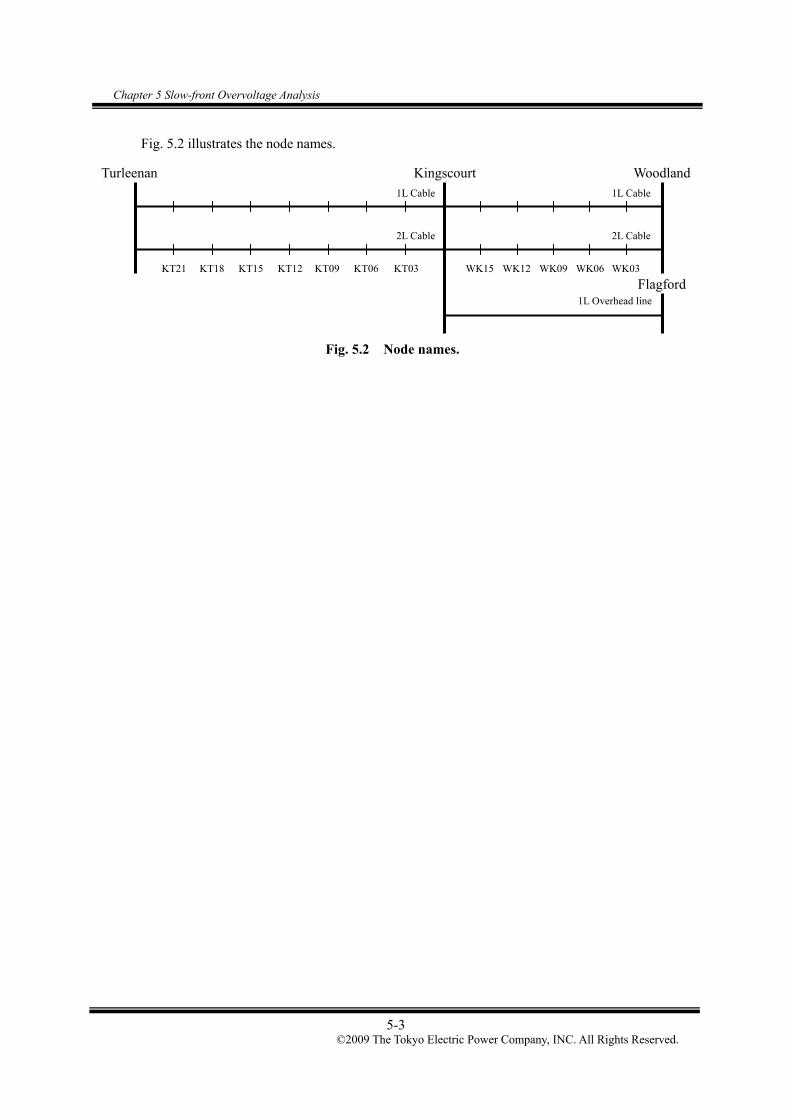
Chapter 5 Slow-front Overvoltage Analysis
5-3 ©2009 The Tokyo Electric Power Company, INC. All Rights Reserved.
Fig. 5.2 illustrates the node names.
Fig. 5.2 Node names.
Turleenan Kingscourt Woodland
Flagford KT21 KT18 KT15 KT12 KT09 KT06 KT03
1L Cable
WK15 WK12 WK09 WK06 WK03
2L Cable
1L Cable
2L Cable
1L Overhead line

Chapter 5 Slow-front Overvoltage Analysis
5-4 ©2009 The Tokyo Electric Power Company, INC. All Rights Reserved.
5.1.1 Results of simulations
The steady state bus voltages when closing the CB were set at around 400 kV in order to
standardize the initial voltage profile. In this study, 200-time simulations were conducted to
realize randomness of the closing switch. According to IEC, the overvoltage was evaluated with
the maximum overvoltage at each node as well as 2 % overvoltage value. The 2 % value is the
twelfth-largest value (200 simulations × 3 phases × 2 % = 12) in the simulation at each node.
The open end terminal produced a larger overvoltage than at other locations due to its positive
reflection in general. In this analysis, the severest overvoltages were observed at the Woodland
cable open end terminal in the energisation of the Kingscourt – Woodland line from Kingscourt
(Case 4). In this case, the maximum overvoltage was 1.86 pu, and the 2 % overvoltage was 1.59
pu, both of which were much lower than SIVW (1050 kV, 3.2 pu).
Table 5-1 Maximum and 2 % Value in the Line Energisation Analysis
(Unit: pu)
Cases Case 1 Case 2 Case 3 Case 4
Energised circuit Kings.-Wood. Turl. –Kings. Turl. –Kings. Kings.-Wood.
Closing CB Woodland Kingscourt Turleenan Kingscourt
Nodes Max. 2 % Max. 2 % Max. 2 % Max. 2 %
Turleenan n/a n/a 1.65 1.54 1.53 1.48 1.30 1.22
KT21 n/a n/a 1.56 1.46 1.54 1.49 1.24 1.22
KT18 n/a n/a 1.44 1.37 1.54 1.50 1.24 1.22
KT15 n/a n/a 1.38 1.30 1.54 1.50 1.24 1.22
KT12 n/a n/a 1.33 1.25 1.53 1.51 1.24 1.22
KT09 n/a n/a 1.26 1.24 1.53 1.51 1.24 1.22
KT06 n/a n/a 1.26 1.23 1.54 1.52 1.24 1.22
KT03 n/a n/a 1.25 1.23 1.55 1.53 1.24 1.22
Kingscourt (Turl.-side) n/a n/a 1.24 1.22 1.55 1.53 1.26 1.22
Kingscourt (Wood.-side) 1.62 1.58 1.24 1.22 n/a n/a 1.23 1.22
WK15 1.61 1.57 1.25 1.22 n/a n/a 1.33 1.24
WK12 1.60 1.56 1.25 1.22 n/a n/a 1.40 1.35
WK09 1.60 1.56 1.25 1.22 n/a n/a 1.57 1.46
WK06 1.57 1.54 1.25 1.22 n/a n/a 1.55 1.49
WK03 1.55 1.52 1.25 1.22 n/a n/a 1.66 1.54
Woodland 1.53 1.47 1.28 1.21 n/a n/a 1.86 1.59

Chapter 5 Slow-front Overvoltage Analysis
5-5 ©2009 The Tokyo Electric Power Company, INC. All Rights Reserved.
)kV 3
2400pu1(
Fig. 5.3 Maximum overvoltage profile in line energisation.
Fig. 5.4 2 % overvoltage profile in line energisation.
0.0
0.5
1.0
1.5
2.0
2.5
3.0
3.5
Turleenan
KT
21
KT
18
KT
15
KT
12
KT
09
KT
06
KT
03
Kingscourt
Turl.-side
Kingscourt
Wood.-side
WK
15
WK
12
WK
09
WK
06
WK
03
Woodland
(pu)
Kingscourt-Woodland from Kingscourt
Kingscourt-Woodland from Woodland
Turleenan-Kingscourt from Turleenan
Turleenan-Kingscourt from Kingscourt
Switching Impulse Withstand Overvoltage 1050kV (3.21pu)
Switching Impulse Withstand Overvoltage 1050kV (3.21pu)

Chapter 5 Slow-front Overvoltage Analysis
5-6 ©2009 The Tokyo Electric Power Company, INC. All Rights Reserved.
5.1.2 Waveform of the maximum overvoltage
The following figure shows the waveform of the maximum overvoltage. The maximum
overvoltage was observed at the Woodland cable open terminal when the Woodland – Kingscourt
line was energised from Kingscourt at the following timings.
Phase Phase A Phase B Phase C
Close timing 18.642 ms 18.049 ms 16.702 ms
Fig. 5.5 Waveform of the maximum overvoltage at the Woodland cable end terminal.
Fig. 5.6 Voltage profile along the Kingscourt-Woodland line.
(file Part2_rev24_close_KW_from_K_wto_FF_max_LG_case.pl4; x-var t) v:WDLD1A v:WDLD1B v:WDLD1C 0 10 20 30 40 50 60 70[ms]
-500
-300
-100
100
300
500
700
[kV]
Woodland cable open end Phase A 607kV
(file Part2_rev24_close_KW_from_K_wto_FF_max_LG_case.pl4; x-var t) v:WDLD1A v:WK121A v:WK061A v:KNGY1A 15 17 19 21 23 25[ms]
-300
-100
100
300
500
700
[kV]Woodland cable open end Phase A 606kV Woodland cable end
WK06 WK12 Kingscourt
Phase C closed at Kings.
Phase B closed at Kings
Phase A closed at Kings

Chapter 5 Slow-front Overvoltage Analysis
5-7 ©2009 The Tokyo Electric Power Company, INC. All Rights Reserved.
5.1.3 Effect of the number of shunt reactors
The number of shunt reactors in service may affect the energisation overvoltage. Four
reduced compensation cases were studied for the Woodland – Kingscourt line in addition to the
original case depicted in Fig. 5.7. The following simulation analyses the effect of it with the
scenario which produced the maximum overvoltage in the previous sections. In the scenario, the
Woodland – Kingscourt line is energised from the Kingscourt side, and Fig. 5.7 shows the
waveforms of the Phase A voltage at the Woodland cable open terminal.
As we can see from the figure, the waveforms just after the energisation are approximately
equal between different compensations. This shows that the number of shunt reactors in service
has small effect on the line energisation overvoltage. The voltage difference of one cycle after
line energisation was caused by the difference compensations, which can also be observed in the
steady-state. It is reasonable to conclude that line energisation is not sensitive to the number of
shunt reactors in service.
Fig. 5.7 Voltage profile along the Kingscourt-Woodland line.
0.00 0.02 0.04 0.06 0.08 0.10 0.12[s]-700
-525
-350
-175
0
175
350
525
700[kV]
15 20 25 30 35 40[ms]-500
-300
-100
100
300
500
700
[kV]Kingscourt Woodland 2120(MVA) 2120(MVA) original 2120(MVA) 1120(MVA) 2120(MVA) 0120(MVA) 1120(MVA) 2120(MVA) 0120(MVA) 2120(MVA)
These voltage differences are observed in the steady-state.
Approximately equal

Chapter 5 Slow-front Overvoltage Analysis
5-8 ©2009 The Tokyo Electric Power Company, INC. All Rights Reserved.
5.2 Ground Fault and Fault Clearing Overvoltage
The slow-front overvoltage caused by ground faults and fault clearings was studied with
different fault timings. The conditions of the analysis are:
Fault point: Seven points in each 400 kV cable route
Fault type: Single line to ground fault (core to sheath) at Phase A
Fault timing: 0° – 170° (10° step – 18 faults)
In this analysis, fault timing was varied because the fault angle was changed from 0° – 170° in
10° steps. The circuit breakers clearing the fault were opened at the first current-zero, 60ms after
the fault occurrence. All three phases were opened at the same time in cable line faults, because
cable lines will not be auto-reclosed. On the other hand, only the faulted phase was opened in
overhead lines.
In this analysis, the simulation was repeated 126 times for each case (= 7 fault points × 18
fault angles). Hence, 2 % value is the seventh largest value (126 simulations × 3 phases × 0.02) in
the simulation at each location.
In general, smaller system modeling yields a larger overvoltage due to its low attenuation and
small number of propagation routes, in which the transient components can be dispersed. Fig. 5.9
illustrates scenarios of the ground fault and fault clearing overvoltage analysis.
The following figure shows the observation nodes and fault nodes used in the simulation.
Fig. 5.8 Node names.
Turleenan Kingscourt Woodland
Flagford KT21 KT18 KT15 KT12 KT09 KT06 KT03
1L Cable
WK15 WK12 WK09 WK06 WK03
2L Cable
1L Cable
2L Cable
1L Overhead line
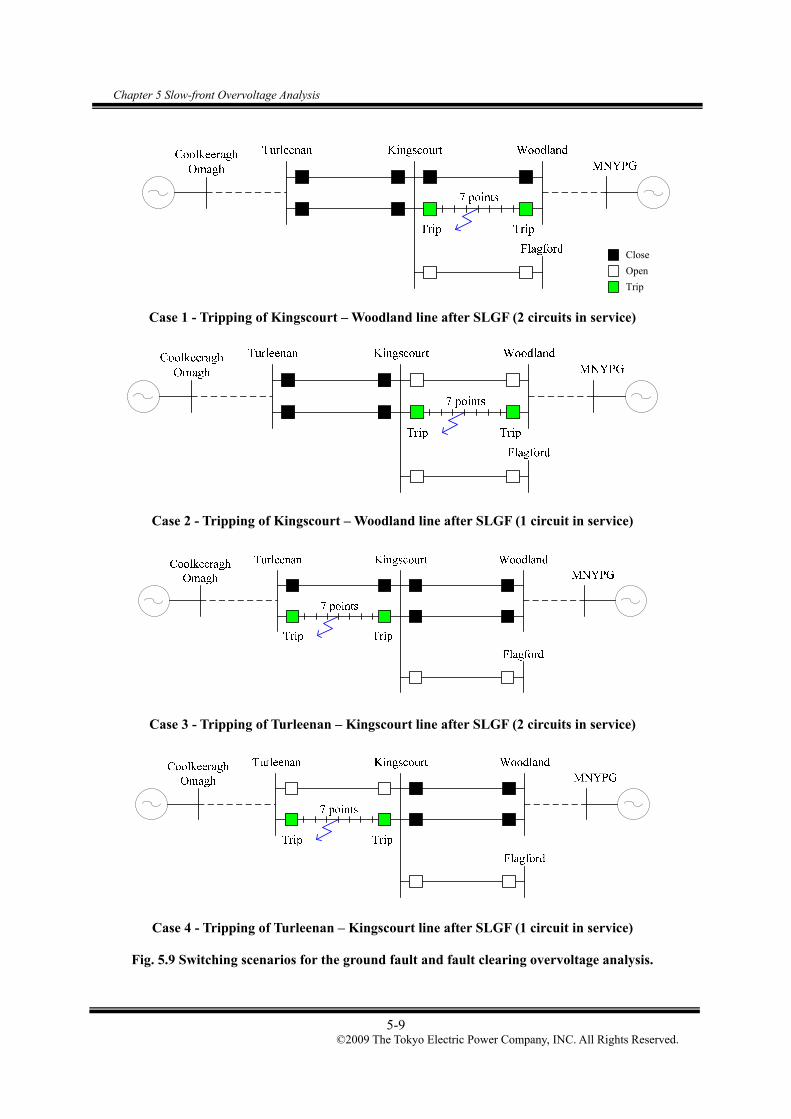
Chapter 5 Slow-front Overvoltage Analysis
5-9 ©2009 The Tokyo Electric Power Company, INC. All Rights Reserved.
Case 1 - Tripping of Kingscourt – Woodland line after SLGF (2 circuits in service)
Case 2 - Tripping of Kingscourt – Woodland line after SLGF (1 circuit in service)
Case 3 - Tripping of Turleenan – Kingscourt line after SLGF (2 circuits in service)
Case 4 - Tripping of Turleenan – Kingscourt line after SLGF (1 circuit in service)
Fig. 5.9 Switching scenarios for the ground fault and fault clearing overvoltage analysis.
Close
Open
Trip

Chapter 5 Slow-front Overvoltage Analysis
5-10 ©2009 The Tokyo Electric Power Company, INC. All Rights Reserved.
5.2.1 Results of simulations
According to IEC, the overvoltage was evaluated with the maximum overvoltage at each node
as well as 2 % overvoltage value. The maximum overvoltage and 2 % overvoltage at each node
are shown in Table 5-2.
Table 5-2 Maximum Overvoltage in the Ground Fault and Fault Clearing Analysis
(Unit: pu)
Cases Case 1 Case 2 Case 3 Case 4
# of circuits (Kings.-Wood.) 21 10 2 2
# of circuits (Turl. –Kings.) 2 2 21 10
Opening CB Kingscourt
Woodland
Kingscourt
Woodland
Turleenan
Kingscourt
Turleenan
Kingscourt
Turleenan 1.64-B-KINGA 1.57-B-KINGA 1.66-B-KINGA 1.82-B-KINGA
KT21 1.64-B-KINGA 1.59-B-KINGA 1.64-B-KINGA 1.75-B-KINGA
KT18 1.65-B-KINGA 1.57-B-KINGA 1.67-B-KINGA 1.76-B-KINGA
KT15 1.51-B-KINGA 1.56-A-KINGA 1.53-B-KINGA 1.76-B-KINGA
KT12 1.47-B-KINGA 1.56-A-KINGA 1.48-B-KT03A 1.61-B-KINGA
KT09 1.52-B-KINGA 1.56-A-KINGA 1.53-B-KINGA 1.54-B-KINGA
KT06 1.61-B-KINGA 1.57-B-KINGA 1.62-B-KINGA 1.54-B-KINGA
KT03 1.66-B-KINGA 1.62-B-KINGA 1.65-B-KINGA 1.47-B-KINGA
Kingscourt (Turl.-side) 1.39-B-WK06A 1.56-A-KINGA 1.38-B-KT15A 1.47-B-KT09A
Kingscourt (Wood.-side) 1.39-B-WK06A 1.43-B-WK03A 1.38-B-KT15A 1.47-B-KT09A
WK15 1.40-B-WK03A 1.47-B-WK03A 1.37-B-KT09A 1.44-B-KT12A
WK12 1.45-B-WK15A 1.47-B-WDLDA 1.39-B-KINGA 1.46-B-KT09A
WK09 1.47-B-WK15A 1.53-B-WK03A 1.42-B-KINGA 1.47-B-KT09A
WK06 1.44-B-WK15A 1.50-B-WK03A 1.44-B-KINGA 1.51-B-KT09A
WK03 1.45-B-KINGA 1.51-B-WK06A 1.44-B-KINGA 1.49-B-KT09A
Woodland 1.52-B-KINGA 1.55-B-KINGA 1.52-B-KINGA 1.54-B-KINGA
Note) X – Y – Z X: Magnitude of overvoltage in per unit (1 pu = 326.6 kV)
Y: Observed phase
Z: Fault node and phase
The highest overvoltage of 1.815 pu was observed in Phase B at the Turleenan bus, when the
fault occurred in Phase A at the Kingscourt-side cable terminal of the Kingscourt – Turleenan line.

Chapter 5 Slow-front Overvoltage Analysis
5-11 ©2009 The Tokyo Electric Power Company, INC. All Rights Reserved.
Table 5-3 2 % Value in the Ground Fault and Fault Clearing Analysis
(Unit: pu)
Cases Case 1 Case 2 Case 3 Case 4
Circuit # of Kings.-Wood. 21 10 2 2
Circuit # of Turl. –Kings. 2 2 21 10
Opening CB Kingscourt
Woodland
Kingscourt
Woodland
Turleenan
Kingscourt
Turleenan
Kingscourt
Turleenan 1.44-B-WK15A 1.55-A-WK15A 1.44-B-TRLTA 1.65-B-KT03A
KT21 1.41-B-WK03A 1.55-A-WK15A 1.38-B-KT03A 1.55-B-KT03A
KT18 1.41-B-KINGA 1.55-A-WK15A 1.39-B-KT06A 1.55-B-KT03A
KT15 1.40-B-WK15A 1.55-A-WK12A 1.41-B-KT03A 1.55-B-KT09A
KT12 1.38-B-WK15A 1.54-A-WK12A 1.39-B-KT15A 1.51-B-KT12A
KT09 1.39-B-WK03A 1.55-A-WK12A 1.38-B-KT03A 1.47-B-KT12A
KT06 1.41-B-WDLDA 1.55-A-WK12A 1.40-B-TRLTA 1.43-B-KT12A
KT03 1.39-B-WK06A 1.55-A-KINGA 1.39-B-KT21A 1.43-B-KT09A
Kingscourt (Turl.-side) 1.36-B-WK03A 1.54-A-WK12A 1.34-B-KT09A 1.41-B-KT18A
Kingscourt (Wood.-side) 1.36-B-WK03A 1.40-B-WK06A 1.34-B-KT09A 1.41-B-KT18A
WK15 1.36-B-WK06A 1.44-B-WK03A 1.33-B-TRLTA 1.41-B-KT06A
WK12 1.39-B-WK12A 1.43-B-WK06A 1.36-B-KINGA 1.41-B-KT12A
WK09 1.40-B-WK15A 1.45-B-WK06A 1.37-B-KT09A 1.42-B-KT18A
WK06 1.40-B-KINGA 1.46-B-WK03A 1.38-B-KT12A 1.44-B-KT06A
WK03 1.41-B-KINGA 1.47-B-WK06A 1.37-B-KT12A 1.43-B-KINGA
Woodland 1.39-B-WDLDA 1.48-B-WK03A 1.38-B-KT09A 1.44-B-KT09A
Note) X – Y – Z X: Overvoltage value in per unit (1pu = 326.6kV)
Y: Observed phase
Z: Fault node and phase
The highest 2 % overvoltage 1.644 pu was observed in Phase B at the Turleenan bus, when the
fault occurred in Phase A at the node KT03 in the Kingscourt – Turleenan line.
Fig. 5.10 shows waveforms of the highest overvoltage of 1.815 pu, and Fig. 5.11 shows
current through CBs on both sides of the line when the highest overvoltage was observed.

Chapter 5 Slow-front Overvoltage Analysis
5-12 ©2009 The Tokyo Electric Power Company, INC. All Rights Reserved.
Case 4 – Overvoltage: 1.82 pu
Fault: Phase A at the Kingscourt-side cable terminal of the Kingscourt – Turleenan line
Maximum overvoltage: Observed in Phase B at the Turleenan bus
Fig. 5.10 Waveform of the maximum overvoltage.
Fig. 5.11 Waveform of fault current.
(file Part2_rev24_clear_TK1_KW2_nonFF_gc_MAX_LG_1_KNGX_1LGS1_A--_100.pl4; x-var t) c:KNGX1A-FAULTP c:TRLT1A-TRLBSA c:TRLT1B-TRLBSB c:TRLT1C-TRLBSC c:KNG4BA-KNGX1A c:KNG4BB-KNGX1B
0.00 0.03 0.06 0.09 0.12 0.15[s]-25
-20
-15
-10
-5
0
5
10
15
[kA]
(file Part2_rev24_clear_TK1_KW2_nonFF_gc_MAX_LG_1_KNGX_1LGS1_A--_100.pl4; x-var t) v:KNGY1A v:KNGY1B v:KNGY1C v:TRLT1A v:TRLT1B v:TRLT1C
0.00 0.03 0.06 0.09 0.12 0.15[s]-600
-400
-200
0
200
400
600
[kV]
Ground fault at Kingscourt in Phase A
Turleenan bus (Phase B): 593kV after the ground fault
Ground fault overvoltage
Fault clearing by tripping CB
Kingscourt bus Phase A: 435kV (clearing)
Fault clearing overvoltage
Fault current Turleenan Phase A Phase B Phase C Kingscourt Phase A Phase B
Phase C24.6kA
Fault clearing by tripping CB

Chapter 5 Slow-front Overvoltage Analysis
5-13 ©2009 The Tokyo Electric Power Company, INC. All Rights Reserved.
1.551.511.511.531.471.471.47
1.561.661.621.561.61
1.761.761.751.82
1.481.471.461.451.431.441.411.541.551.551.551.541.551.551.55
1.65
0.0
0.5
1.0
1.5
2.0
2.5
3.0
3.5
Turleenan
KT
21
KT
18
KT
15
KT
12
KT
09
KT
06
KT
03
Kingscourt T
url-side
Kingscourt W
ood-side
WK
15
WK
12
WK
09
WK
06
WK
03
Woodland
(pu)
Maximum
2%
Fig. 5.12 Maximum overvoltage and 2 % overvoltage in the ground fault and fault clearing.
Fig. 5.12 shows the overall maximum and 2 % overvoltage in the ground fault and fault
clearing analysis. The maximum overvoltage of 1.82 pu and the 2 % overvoltage of 1.65 pu were
observed at the Turleenan bus. The single line to ground fault produced a much higher
overvoltage than the fault clearing as shown in Fig. 5.10, but both of them were much lower than
SIWV of 400 kV equipment.
Switching Impulse Withstand Overvoltage 1050kV (3.21pu)

Chapter 5 Slow-front Overvoltage Analysis
5-14 ©2009 The Tokyo Electric Power Company, INC. All Rights Reserved.
5.3 Conclusion
Slow-front overvoltage caused by line energisation, ground fault, and fault clearing was
studied in this chapter. The result of the slow-front overvoltage analysis is summarized in Table
5-4. As shown in the table, no significant overvoltage was found in the slow-front overvoltage
analysis. The observed overvoltages were much lower than SIWV in all simulated cases.
Table 5-4 Summary of the Slow-front Overvoltage Analysis
Highest overvoltage
(peak)
Withstand voltage (peak)
for evaluation
Line energisation 607.0 kV (1.86 pu)
Ground fault and fault clearing 593.0 kV (1.82 pu) 1050 kV
(peak) 3
2kV 400pu 1

Part 3

Part 3:
Feasibility Study on the 400 kV Woodland –
Kingscourt – Turleenan Line as Mixed OHL /
Underground Cable

Table of contents
©2009 The Tokyo Electric Power Company, INC. All Rights Reserved.
Table of contents
CHAPTER 1 INTRODUCTION _________________________________________________ 1-1
CHAPTER 2 REACTIVE POWER COMPENSATION _____________________________ 2-1
2.1 Proposed Compensation Patterns __________________________________________ 2-1
2.2 Ferranti Phenomenon ___________________________________________________ 2-2
2.3 Resonance Overvoltage in an Opened Phase _________________________________ 2-6
2.4 Conclusion __________________________________________________________ 2-10
CHAPTER 3 MODEL SETUP __________________________________________________ 3-1
3.1 Combinations of OHLs and Underground Cables _____________________________ 3-1
3.2 Shunt Reactors ________________________________________________________ 3-2
CHAPTER 4 TEMPORARY OVERVOLTAGE ANALYSIS __________________________ 4-1
4.1 Conditions for the Parallel Resonance Overvoltage Analysis_____________________ 4-1
4.2 Parallel Resonance Frequency Seen from Kingscourt 400 kV ____________________ 4-4
4.3 Overvoltage Caused by the System Islanding________________________________ 4-13
4.4 Conclusion __________________________________________________________ 4-17
CHAPTER 5 OVERVOLTAGE CAUSED BY AUTORECLOSE _____________________ 5-17
5.1 Simulation conditions __________________________________________________ 5-17
5.2 Residual Voltage in Typical Operation _____________________________________ 5-17
5.3 Effect of Fault Clearing Timing on Residual Voltage __________________________ 5-17
5.4 Reclosing Timing _____________________________________________________ 5-17
5.5 Simulation Results ____________________________________________________ 5-17
5.6 Three Phase Autoreclose________________________________________________ 5-17
5.7 Conclusion __________________________________________________________ 5-17
CHAPTER 6 LIGHTNING OVERVOLTAGE ____________________________________ 6-17
6.1 Overview____________________________________________________________ 6-17
6.2 Model Setup _________________________________________________________ 6-17
6.3 Result of the Analysis __________________________________________________ 6-17
6.4 Conclusion __________________________________________________________ 6-17

Chapter 1 Introduction
1-1 ©2009 The Tokyo Electric Power Company, INC. All Rights Reserved.
Chapter 1 Introduction
The objective of Part 3 is to conduct feasibility study on the 400 kV Woodland – Kingscourt –
Turleenan line as mixed OHL / underground cable. In order to fulfill this objective, the following
studies were performed:
(1) Transmission Capacity Calculation
(2) Impedance and Admittance Calculation
(3) Reactive Power Compensation Analysis
(4) Overvoltage Analysis
Here, (1) and (2) have already been conducted as a common study for Part 1, 2, and 3 and are
not included in this Part 3 report. Using cable information, such as cable size, type, layout, and
impedance / admittance, found in (1) and (2), the remaining studies (3) and (4) were conducted as
Part 3 studies.
The purpose of (3) is to find shunt reactors that should be installed together with the 400 kV
cable. The best combination in terms of the number of shunt reactors, shunt reactor size, and
location was found from (3).
Temporary overvoltage analysis in (4) is the most important study in Part 3 that addresses the
feasibility of the 400 kV Woodland – Kingscourt – Turleenan line as mixed OHL / underground
cable. In addition to it, overvoltage caused by autoreclose and lightning overvoltage were studied
in (4). These overvoltages are usually not studied when the line is composed of underground
cables for the entire length and are thus peculiar for the mixed OHL / underground cable line.

Chapter 2 Reactive Power Compensation
2-1 ©2009 The Tokyo Electric Power Company, INC. All Rights Reserved.
Chapter 2 Reactive Power Compensation
2.1 Proposed Compensation Patterns
In Part 3, the 400 kV Woodland – Kingscourt line was assumed to be an overhead line, and the
400 kV Kingscourt – Turleenan line was assumed to be a mixed OHL / underground cable. In
order to find effects of the ratio of the cable part, the following combinations were considered for
the Kingscourt – Turleenan line:
Underground cable
(Al 1400 mm2 2 cct)
OHL
(1 cct)
30 % 70 %
60 % 40 %
For each cable ratio, 30% and 60% charging capacity of the Kingscourt – Turleenan line was
calculated at 400 kV as follows:
Cable section OHL section Total
Cable ratio 30 % 457.4 MVA 32.1 MVA 489.5 MVA
Cable ratio 60 % 914.8 MVA 18.3 MVA 933.1 MVA
Based on the maximum unit size found in Part 2, the following reactive power compensation
patterns were proposed. Shunt reactor stations were not proposed:
Table 2.1 Proposed Compensation Patterns
Locations Cable ratio 30 % Cable ratio 60 %
Kingscourt
Turleenan
100 MVA × 2
100 MVA × 2
200 MVA × 2
200 MVA × 2
Compensation Rate [%] 81.7 85.7
The compensation rates were lower compared to those in Part 2 in order to avoid a resonance
overvoltage which occurs when one line is opened for single phase autoreclose. This will be
discussed in Section 2.3.
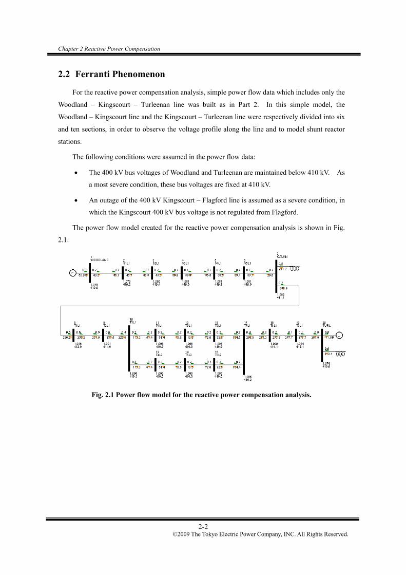
Chapter 2 Reactive Power Compensation
2-2 ©2009 The Tokyo Electric Power Company, INC. All Rights Reserved.
2.2 Ferranti Phenomenon
For the reactive power compensation analysis, simple power flow data which includes only the
Woodland – Kingscourt – Turleenan line was built as in Part 2. In this simple model, the
Woodland – Kingscourt line and the Kingscourt – Turleenan line were respectively divided into six
and ten sections, in order to observe the voltage profile along the line and to model shunt reactor
stations.
The following conditions were assumed in the power flow data:
The 400 kV bus voltages of Woodland and Turleenan are maintained below 410 kV. As
a most severe condition, these bus voltages are fixed at 410 kV.
An outage of the 400 kV Kingscourt – Flagford line is assumed as a severe condition, in
which the Kingscourt 400 kV bus voltage is not regulated from Flagford.
The power flow model created for the reactive power compensation analysis is shown in Fig.
2.1.
Fig. 2.1 Power flow model for the reactive power compensation analysis.

Chapter 2 Reactive Power Compensation
2-3 ©2009 The Tokyo Electric Power Company, INC. All Rights Reserved.
2.2.1 Cable ratio 30 %
First, the reactive power compensation for cable ratio 30 % was studied. In Fig. 2.2, the
black line shows the voltage profile when all equipment is in service and the Woodland –
Kingscourt – Turleenan line is carrying no load. The voltage profile in this condition is
satisfactory. The voltage along the line does not exceed 420 kV.
The other lines in Fig. 2.2 shows the voltage profile when the Turleenan terminal is opened.
When two 100 MVA shunt reactors are directly connected to the line at the open end (red line), the
highest voltage along the line is 420.5 kV, and the voltage profile is acceptable. When only one
100 MVA shunt reactor is directly connected to the line at the open end (blue line), the highest
voltage exceeds 426 kV, but the voltage rise from the Kingscourt 400 kV bus is within 10 kV. The
voltage profile is still permissible as long as the Kingscourt 400 kV bus voltage is maintained
below 410 kV. When no shunt reactors are connected to the line at the open end (purple line), the
voltage profile is hardly acceptable.
410
414
418
422
426
430
434
WO
OD
LA
ND T2
T4
KIN
GSC
OU
RT T7
T9
T11
T13
TU
RL
Vol
tage
[kV
]
No LoadTurleenan Open (200MVA)Turleenan Open (100MVA)Turleenan Open (No Reactor)
Fig. 2.2 Voltage profile when the Turleenan terminal is opened (cable ratio 30 %).

Chapter 2 Reactive Power Compensation
2-4 ©2009 The Tokyo Electric Power Company, INC. All Rights Reserved.
Fig. 2.3 shows the voltage profile when the Kingscourt terminal is opened. As in Fig. 2.2,
the different colors (red, blue, and purple) stand for the different amount of shunt reactors
connected to the line at the open end. When at least one 100 MVA shunt reactor is connected to
the line at the open end, the voltage along the line is maintained below 420 kV.
410
414
418
422
426
KIN
GSC
OU
RT T6
T7
T8
T9
T10
T11
T12
T13
T14
TU
RL
Vol
tage
[kV
]
Kingscourt Open (200MVar)
Kingscourt Open (100MVar)
Kingscourt Open (No Reactor)
Fig. 2.3 Voltage profile when the Kingscourt terminal is opened (cable ratio 30 %).
2.2.2 Cable ratio 60 %
Next, the reactive power compensation for cable ratio 60 % was studied. In Fig. 2.4, the
black line shows the voltage profile when all equipment is in service and the Woodland –
Kingscourt – Turleenan line carries no load. The voltage profile in this condition is satisfactory.
The voltage along the line does not exceed 420 kV.
The other lines in Fig. 2.4 shows the voltage profile when the Turleenan terminal is opened.
When the two 200 MVA shunt reactors are directly connected to the line at the open end (red line),
the highest voltage along the line is 424.3 kV, but the voltage rise from the Kingscourt 400 kV bus
is within 10 kV. The voltage profile is still acceptable as long as the Kingscourt 400 kV bus
voltage is maintained below 410 kV. When only one of the 200 MVA shunt reactors is directly
connected to the line at the open end (blue line), the highest voltage is 435.6 kV. The voltage rise
from the Kingscourt 400 kV bus is 15 kV. When no shunt reactors are connected to the line at the
open end (purple line), the voltage profile is hardly acceptable.
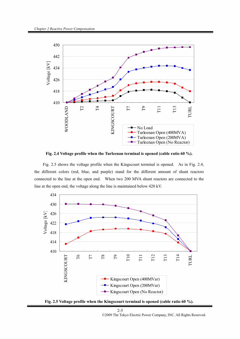
Chapter 2 Reactive Power Compensation
2-5 ©2009 The Tokyo Electric Power Company, INC. All Rights Reserved.
410
418
426
434
442
450
WO
OD
LA
ND T2
T4
KIN
GSC
OU
RT T7
T9
T11
T13
TU
RL
Vol
tage
[kV
]
No LoadTurleenan Open (400MVA)Turleenan Open (200MVA)Turleenan Open (No Reactor)
Fig. 2.4 Voltage profile when the Turleenan terminal is opened (cable ratio 60 %).
Fig. 2.5 shows the voltage profile when the Kingscourt terminal is opened. As in Fig. 2.4,
the different colors (red, blue, and purple) stand for the different amount of shunt reactors
connected to the line at the open end. When two 200 MVA shunt reactors are connected to the
line at the open end, the voltage along the line is maintained below 420 kV.
410
414
418
422
426
430
434
KIN
GSC
OU
RT T6
T7
T8
T9
T10
T11
T12
T13
T14
TU
RL
Vol
tage
[kV
]
Kingscourt Open (400MVar)
Kingscourt Open (200MVar)
Kingscourt Open (No Reactor)
Fig. 2.5 Voltage profile when the Kingscourt terminal is opened (cable ratio 60 %).

Chapter 2 Reactive Power Compensation
2-6 ©2009 The Tokyo Electric Power Company, INC. All Rights Reserved.
2.3 Resonance Overvoltage in an Opened Phase
When charging capacity of an overhead line or a mixed OHL / underground cable is
compensated by line-connected shunt reactors, resonance overvoltage can occur in the faulted
phase if this phase is opened for single phase autoreclose. This resonance overvoltage often poses
a limitation to the compensation rate achievable, and it is necessary to study so that the resonance
overvoltage does not occur in the proposed compensation patterns.
When shunt reactors are connected to the bus (not to the line), they are disconnected from the
faulted (open) line when the fault is cleared. Thus, resonance overvoltage does not occur without
inductance of shunt reactors. Additionally, when the line is composed of the underground cable
for its entire length, resonance overvoltage does not occur since mutual capacitance between
faulted phase and healthy phases does not exist.
The ATP-EMTP simulation model as shown in Fig. 2.6 was built for the resonance
overvoltage analysis. The simulation model includes only the Kingscourt – Turleenan line, and
both ends of the line were fixed to 400 kV by voltage sources.
KING4 KT001 TURL4
24.6km
GROUPkin-tur
100MVar
GROUPreactor
LCC
14.35 km
V LCC
14.35 km
LCC
14.35 km
KT121KT131LCC
14.35 km
V V V
24.6kmKT001
KT091
GROUPkin-tur
100MVar
GROUPreactor
Fig. 2.6 Simulation model for the resonance overvoltage analysis.
Fig. 2.7 shows the result of the resonance overvoltage analysis for cable ratio 30 %. For the
analysis, circuit breakers of Phases A, B, and C were opened one by one. In the figure, red, green,
and blue lines are the voltages of the opened phase A, B, and C, respectively.

Chapter 2 Reactive Power Compensation
2-7 ©2009 The Tokyo Electric Power Company, INC. All Rights Reserved.
part3_30per_resonancea.pl4: v:KT101A part3_30per_resonanceb.pl4: v:KT101B part3_30per_resonancec.pl4: v:KT101C
40 44 48 52 56 60[Hz]0
100
200
300
400
500
600
[kV]
Fig. 2.7 Result of resonance overvoltage analysis (cable ratio 30 %).
Resonance frequencies were found between 45.2 Hz and 45.4 Hz, which was out of the normal
operating range. The voltage of the faulted phase was reasonably low in the normal operating
range.
Then, the resonance overvoltage analysis was performed for higher compensation rates. The
red line in Fig. 2.8 corresponds to the proposed compensation pattern. Green and blue lines
correspond to higher compensation rates as shown in the table below. It can be seen that the
resonance frequency shifts closer to the normal operating range for a higher compensation rate.
The proposed compensation pattern is considered safe, but the green line can be a little risky
considering errors in the simulation and manufacture of equipment. The blue line is not
acceptable since the resonance frequency (49.4 Hz) is too close to nominal frequency.
1 pu

Chapter 2 Reactive Power Compensation
2-8 ©2009 The Tokyo Electric Power Company, INC. All Rights Reserved.
part3_30per_resonancea.pl4: v:KT101A part3_30per_resonancea_120mvar.pl4: v:KT101A part3_30per_resonancea_120mvar2.pl4: v:KT101A
40 44 48 52 56 60[Hz]0
100
200
300
400
500
600
[kV]
Kingscourt Turleenan Compensation rate Resonance frequency
Red line 100 MVA × 2 100 MVA × 2 81.7 % 45.4 Hz
Green line 100 MVA × 2 120 MVA × 2 89.9 % 47.4 Hz
Blue line 120 MVA × 2 120 MVA × 2 98.1 % 49.4 Hz
Fig. 2.8 Result of resonance overvoltage analysis for higher compensation rates.
1 pu

Chapter 2 Reactive Power Compensation
2-9 ©2009 The Tokyo Electric Power Company, INC. All Rights Reserved.
There are two countermeasures that can be utilized if it is necessary to achieve a reactive
power compensation rate closer to 100 % in order to control the voltage profile and reactive power
flow in the network and to prevent harmful overvoltages.
One of the countermeasures is to adopt four-legged shunt reactors. By the adoption of
four-legged shunt reactors, it is possible to shift the resonance frequency. Fig. 2.9 compares the
result of the analysis with the four-legged shunt reactors (green line) and the normal shunt reactors
(red line). Compensation rate was fixed at 98.1 % (Kingscourt: 120 MVA × 2, Turleenan: 120
MVA × 2). For the four-legged shunt reactors, impedance of the grounding reactor was set to
1000 mH.
As shown in Fig. 2.9, it was confirmed that the resonance frequency was shifted from 49.4 Hz
to 46.0 Hz by adopting four-legged shunt reactors. However, the open phase voltage at the
resonance frequency became very high. The normal operating range is far away from 46 Hz, but
the open phase voltage is higher than 1 pu even at 49 Hz. This result implies that careful attention
is necessary when adopting four-legged shunt reactors in order to shift the resonance frequency.
part3_30per_resonancea_120mvar2.pl4: v:KT101A part3_30per_resonancea_120mvar2_4leg.pl4: v:KT101A
40 44 48 52 56 60[Hz]0
2
4
6
8
10
12
[MV]
Fig. 2.9 Result of resonance overvoltage analysis with four-legged shunt reactors.
The other countermeasure is to adopt three phase autoreclose instead of single phase
autoreclose. Reliability of the interconnector is undermined by this change, but open phase
resonance does not occur since all three phases are opened even in single line to ground faults.
Overvoltages caused by autoreclose become more severe for three phase autoreclose compared to

Chapter 2 Reactive Power Compensation
2-10 ©2009 The Tokyo Electric Power Company, INC. All Rights Reserved.
single phase autoreclose as explained in Chapter 4.
The resonance overvoltage analysis was also performed for cable ratio 60 %. In the proposed
compensation pattern, the resonance frequency was found at 45.6 Hz for the faulted phases A, B,
and C. Although resonance overvoltage was lower than 1 pu, it is not recommended to increase
the compensation rate.
part3_60per_resonancea.pl4: v:KT151A part3_60per_resonanceb.pl4: v:KT151B part3_60per_resonancec.pl4: v:KT151C
40 44 48 52 56 60[Hz]0
50
100
150
200
250
300
[kV]
Fig. 2.10 Result of resonance overvoltage analysis (cable ratio 60 %).
2.4 Conclusion
As a result of the reactive power compensation analysis, the proposed compensation patterns
were found to be satisfactory even when one terminal of the line was opened as long as all shunt
reactors were connected to the line at the open terminal.
For cable ratio 30 %, one 100 MVA shunt reactor can be connected to the bus instead of the
line, but it is recommended to connect both shunt reactors to the line considering a potential outage
of the shunt reactor.
For cable ratio 60%, both 200 MVA shunt reactors have to be connected to the line in order to
maintain the voltage below 420 kV. When one shunt reactor is not available, the voltage at the
open end can be higher than the other end by 15 kV. This can be an acceptable risk, but it is
preferable to conduct maintenance of the line and the shunt reactor at the same time.

Chapter 2 Reactive Power Compensation
2-11 ©2009 The Tokyo Electric Power Company, INC. All Rights Reserved.
Additionally, the resonance overvoltage analysis was carried out, and the proposed
compensation patterns were found to be safe when any faulted phase was opened for single phase
autoreclose.
In conclusion, the proposed compensation patterns shown below will be used for further
analysis in Part 3.
Locations Cable ratio 30 % Cable ratio 60 %
Kingscourt
Turleenan
100 MVA × 2
100 MVA × 2
200 MVA × 2
200 MVA × 2
Compensation Rate [%] 81.7 85.7

Chapter 3 Model Setup
3-1 ©2009 The Tokyo Electric Power Company, INC. All Rights Reserved.
Chapter 3 Model Setup
3.1 Combinations of OHLs and Underground Cables
The following combinations of OHLs and underground cables as shown in Fig. 3.1 were
studied in Part 3. The cable section was placed at the Kingscourt end or in the center of the 400
kV Kingscourt – Turleenan line. The location and amount of shunt reactors in the figure reflect
the results of the reactive power compensation analysis in Chapter 1.
Fig. 3.1 Combinations of OHLs and underground cables for the Kingscourt – Turleenan line.

Chapter 3 Model Setup
3-2 ©2009 The Tokyo Electric Power Company, INC. All Rights Reserved.
Additionally for the analysis of the overvoltage caused by autoreclose, another setup as shown
in Fig. 3.2 was studied in order to determine the effect of different shunt reactor locations.
Fig. 3.2 Additional combination of OHLs and underground cables for the Kingscourt – Turleenan line.
Other models – such as OHL models, transformer models, surge arrester models, generator
models, and load models – are the same as those in Part 2. Explanations of these models are given
in Part 2 of the report. Since 200 MVA shunt reactors are used only in Part 3, explanations on
shunt reactor models are given here.
3.2 Shunt Reactors
Shunt reactors were connected to both ends of the 400 kV cables or 400 kV buses, in order to
compensate charging capacity of the cables. Shunt reactors for the Kingscourt – Turleenan line
were modeled as shown in Fig. 3.1 and Fig. 3.2. 400 kV shunt reactors in the simulation model
are shown in Table 3.1.
Table 3.1 400 kV Shunt Reactors in the Simulation Model
Kingscourt – Turleenan (82 km) Kingscourt: 100 or 200 MVA × 2
Turleenan: 100 or 200 MVA × 2
Woodland – Oldstreet (125 km) Woodland: 80 MVA × 1
Moneypoint – Tarbert (6.5 km) Moneypoint: 50 MVA × 1
Tarbert: 50 MVA × 1
When 400 kV shunt reactors are close to the point of interest, they are modeled with the
saturation characteristics. Otherwise they are modeled as linear inductances.

Chapter 4 Temporary Overvoltage Analysis
4-1 ©2009 The Tokyo Electric Power Company, INC. All Rights Reserved.
Chapter 4 Temporary Overvoltage Analysis
For long EHV cables, temporary overvoltages are of highest concerns in terms of the safe
operation after the installation. Highest temporary overvoltages are often higher than highest
slow-front overvoltages.
Due to the large capacitance associated with the long EHV cable and the inductance of shunt
reactors for the reactive power compensation, the following temporary overvoltages require a close
attention for the network with long EHV cables:
(1) Parallel resonance overvoltage
(2) Oscillatory overvoltage caused by the system islanding
For equipment whose highest voltage is higher than 245 kV, the standard short-duration
power-frequency withstand voltage is not specified in IEC, but it is specified by a utility or a
manufacturer. Surge arresters are generally the weakest among different equipment. The
temporary overvoltages have to be evaluated against typical withstand voltage and energy
absorption capability of surge arresters. Note that the temporary overvoltages may be evaluated
with SIWV depending on their decay time.
4.1 Conditions for the Parallel Resonance Overvoltage Analysis
Parallel resonance frequencies were found from the results of a frequency scan in EMTP as
shown in Fig. 4.1.
Parallel resonance frequency seen from the Kingscourt substation
Fig. 4.1 Frequency sweep for the parallel resonance overvoltage analysis.

Chapter 4 Temporary Overvoltage Analysis
4-2 ©2009 The Tokyo Electric Power Company, INC. All Rights Reserved.
Since the focus of the parallel resonance overvoltage analysis in Part 3 is to find the effect of
the partial cabling on parallel resonance, the following conditions were fixed in Part 3 in
consideration of the result of the parallel resonance overvoltage analysis conducted in Part 2:
Since impedance of the network seen from the Woodland, Kingscourt, and Turleenan
400 kV were similar, the analysis in Part 3 focused on impedance seen from Kingscourt
400 kV.
The 400 kV Kingscourt – Flagford line and the 400 kV Woodland – Oldstreet line were
assumed to be out of service in order to yield a larger magnitude of impedance at the
parallel resonance frequency.
Source impedances of dummy generators connected to the Woodland 220 kV, the Kingscourt
220 kV, and the Turleenan 275 kV buses were adjusted to shift the parallel resonance frequency to
100 Hz. After the frequency scan, the time domain simulation was conducted under the most
severe conditions as shown in Fig. 4.2.
Fig. 4.2 Sample scenario of the time domain simulation for the parallel resonance overvoltage
analysis.
Close
Open
On

Chapter 4 Temporary Overvoltage Analysis
4-3 ©2009 The Tokyo Electric Power Company, INC. All Rights Reserved.
In the parallel resonance overvoltage analysis, an effect of the fault current level (source
impedance) at the Woodland 220 kV, the Kingscourt 220 kV, and the Turleenan 275 kV buses was
studied as one of parameters. In order to find the reasonable range for this parameter, the fault
current calculation was performed at these buses in Part 2.
Generators included in the simulation model are fewer than those in service in summer
off-peak power flow data. An adjustment of the fault current level can be achieved by adding a
dummy source with different source impedances. Based on the fault current calculation result in
Part 2, the source impedance values were varied in the range shown below.
Table 4.1 Assumed Range of Source Impedance Values
Woodland 220 kV 20 – 60 mH
Kingscourt 220 kV 40 – 60 mH
Turleenan 275 kV 20 – 50 mH

Chapter 4 Temporary Overvoltage Analysis
4-4 ©2009 The Tokyo Electric Power Company, INC. All Rights Reserved.
4.2 Parallel Resonance Frequency Seen from Kingscourt 400 kV
Parallel resonance frequency of the network seen from Kingscourt 400 kV was found by a
frequency scan based on the simulation model in Fig. 4.3.
WDLD4LCC
125. km
MNPT4 OLDS4LCC
105. km
WMDL4
LCC
85. km
LAOI4LCC
85.23 km
DNST4LCC
44.77 km
24.6km
GR
OU
Pki
n-tu
r
100MVar
GROUPreactor
100MVar
GROUPreactor
50mH
60mH
KT091
LCC
14.3
5 km
60mH
KT101
LCC
14.3
5 km
KT111
LCC
14.3
5 km
KT121
LCC
14.3
5 km
U
Load
KELL4
LCC
60.
km
SAT
Y Y
SAT
Y Y
SAT
Y Y
SAT
Y Y
SAT
Y Y
SAT
Y Y
24.6km
KING4
KT091
GR
OU
Pki
n-tu
r
WDLD2Y Y
I-Phi
Y Y
I-Phi
OLDS2
standard
YY
WMDL2
standard
YYLAOI2
standard
YY
59.3km
401.2L4.193
V
410.2L5.575
V
402.8L6.963
V
GROUPturl tr
MNYPGSAT
Y Y
TRBT1SAT
Y Y
SAT
Y Y
standard
YY
standard
YY
BLLC2
DM136
SA
T
YY
50MVA
50MVATRBT4
KING4 KING2Y Y
I-Phi
FLAG4LCC
60. km
GROUPturl tr
KELL2
standard
YY
LCC
9.6
7 km
WK011
LCC
9.67
km
WK021
LCC
9.67
km
WK031
LC
C
9.6
7 km
WK041
LCC
9.67
km
WK051
LCC
9.67
km
U
U
U
U
U
U
U
FLAG2
standard
YY
DNST2
standard
YYTRBT2
standard
YY
ABC 56.09km
216.9L2.246V
123km
90km
20kmLOUT2
61km
18.43kmCORD2
17.83km
4.5kmHNST2
3.73km
1.4kmFING2
LOUTX
SAT
Y Y
SAT
Y Y
LOUTYSAT
Y Y
50km 50km
TAND2
19.94km
TURL4 TURL2GROUP
turl tr
42km
5.63km
31.69km
26.04km
TAMN2
MAGF2
56.09km
0.2kmCAC2A
0.17kmCAC2B
COOL2
60km
OMAH2
25kmSTRB2
224.1L5.876
V
412.2L5.793
V
400.9L4.474
V
407.6L4.694V
Load
Load
Load
Load
Load
Load
Load
Load
100MVar
GROUPreactor
GROUPreactor
22.5km
WDLD2
30.55kmMYNT2
6.5km
GROUPmp-tb
GROUPmp-tb
100MVar
GROUPreactor
1A
80MVar
Reactor 80MVar
Dummy source
Dummy source
Dummy source
Fig. 4.3 Simulation model for a frequency scan seen from Kingscourt 400 kV.
Current source (1 Amp)
Kingscourt – Turleenan line
Woodland – Kingscourt line
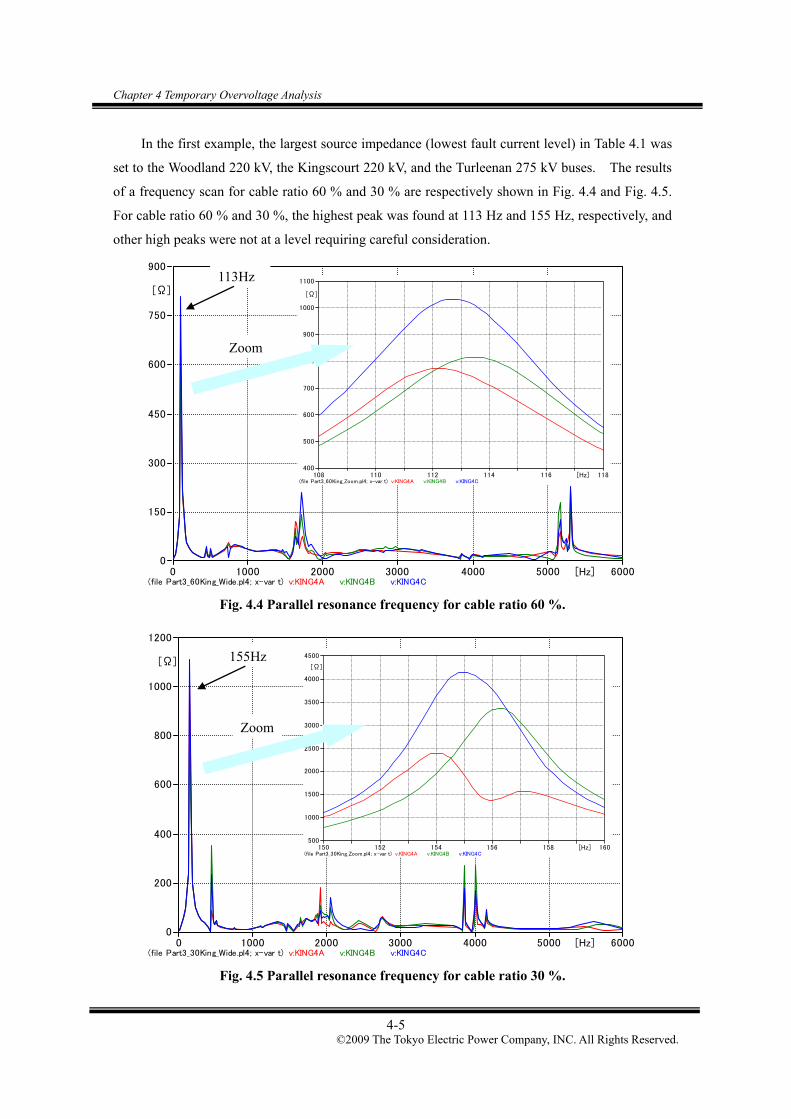
Chapter 4 Temporary Overvoltage Analysis
4-5 ©2009 The Tokyo Electric Power Company, INC. All Rights Reserved.
In the first example, the largest source impedance (lowest fault current level) in Table 4.1 was
set to the Woodland 220 kV, the Kingscourt 220 kV, and the Turleenan 275 kV buses. The results
of a frequency scan for cable ratio 60 % and 30 % are respectively shown in Fig. 4.4 and Fig. 4.5.
For cable ratio 60 % and 30 %, the highest peak was found at 113 Hz and 155 Hz, respectively, and
other high peaks were not at a level requiring careful consideration.
(file Part3_60King_Wide.pl4; x-var t) v:KING4A v:KING4B v:KING4C 0 1000 2000 3000 4000 5000 6000[Hz]
0
150
300
450
600
750
900
[Ω]
Fig. 4.4 Parallel resonance frequency for cable ratio 60 %.
(file Part3_30King_Wide.pl4; x-var t) v:KING4A v:KING4B v:KING4C 0 1000 2000 3000 4000 5000 6000[Hz]
0
200
400
600
800
1000
1200
[Ω]
Fig. 4.5 Parallel resonance frequency for cable ratio 30 %.
Zoom
155Hz
(file Part3_30King_Zoom.pl4; x-var t) v:KING4A v:KING4B v:KING4C 150 152 154 156 158 160[Hz]
500
1000
1500
2000
2500
3000
3500
4000
4500
[Ω]
113Hz
(file Part3_60King_Zoom.pl4; x-var t) v:KING4A v:KING4B v:KING4C 108 110 112 114 116 118[Hz]
400
500
600
700
800
900
1000
1100
[Ω]
Zoom

Chapter 4 Temporary Overvoltage Analysis
4-6 ©2009 The Tokyo Electric Power Company, INC. All Rights Reserved.
With the largest source impedance (lowest fault current level), the parallel resonance
frequency and the magnitude of impedance changed with the cable ratio as shown in Table 4.2.
Table 4.2 Magnitude of Impedance at the Parallel Resonance Frequency
Parallel resonance
frequency
Magnitude of
impedance
Cable ratio 100%
(from Part 2 for reference) 86.9 Hz 933 Ω
Cable ratio 60 % 113 Hz 1034 Ω
Cable ratio 30% 155 Hz 4145 Ω
As a result, an energisation of the Kingscourt 400/220 kV transformer was considered to be
the most critical source of harmonic current injection. For each cable ratio, the source impedance
at the Woodland 220 kV and Turleenan 275 kV buses were adjusted in order to yield the parallel
resonance frequency at 100 Hz for cable ratio 60%. For cable ratio 30 %, it seems more
reasonable to shift the parallel resonance frequency to 150 Hz since third harmonic is also
contained in transformer inrush current. The value of this source impedance and the magnitude of
impedance at the parallel resonance frequency are shown in Table 4.3.
Table 4.3 Magnitude of Impedance at the Parallel Resonance Frequency
Source impedance
Turleenan Woodland
Parallel resonance
frequency
Magnitude of
impedance
Cable ratio 100%
(from Part 2 for reference) 20.0 mH 24.8 mH 100 Hz 2606 Ω
Cable ratio 60 % 120 mH 112 mH 100 Hz 849 Ω
Cable ratio 30% 77 mH 70 mH 150 Hz 2692 Ω
In order to shift the parallel resonance frequency to 100 Hz or 150 Hz, it was necessary to set
the values of the source impedance at the Kingscourt 220 kV and the Turleenan 275 kV buses much
higher than their designated reasonable range.

Chapter 4 Temporary Overvoltage Analysis
4-7 ©2009 The Tokyo Electric Power Company, INC. All Rights Reserved.
Finally, a time domain simulation was carried out for both cable ratio 60 % and 30 %. For
cable ratio 60 %, the voltage of the Kingscourt 400 kV bus and inrush current into the Kingscourt
400/220 kV transformer are shown in Fig. 4.6 and Fig. 4.7. The highest voltage observed at the
Kingscourt 400 kV bus was 436.3 kV (1.34 pu) in Phase C. This is not a concern in terms of the
operation of the 400 kV Woodland – Kingscourt – Turleenan line.
(file Inrush_Part3_60King_100Hz.pl4; x-var t) v:KING4A v:KING4B v:KING4C 0.0 0.2 0.4 0.6 0.8 1.0[s]
-500
-375
-250
-125
0
125
250
375
500
[kV]
Fig. 4.6 Kingscourt 400 kV bus voltage in transformer inrush for cable ratio 60 %.
(file Inrush_Part3_60King_100Hz.pl4; x-var t) c:KING4A-KC_TRA c:KING4B-KC_TRB c:KING4C-KC_TRC 0.00 0.04 0.08 0.12 0.16 0.20[s]
-3500
-2500
-1500
-500
500
1500
2500
3500
4500
[A]
Fig. 4.7 Inrush current into the Kingscourt 400/220 kV transformer for cable ratio 60 %.

Chapter 4 Temporary Overvoltage Analysis
4-8 ©2009 The Tokyo Electric Power Company, INC. All Rights Reserved.
For cable ratio 30 %, the voltage of the Kingscourt 400 kV bus and inrush current into the
Kingscourt 400/220 kV transformer are shown in Fig. 4.8 and Fig. 4.9. The highest voltage
observed at the Kingscourt 400 kV bus was 604.2 kV (1.85 pu) in Phase C. Since the resonance
frequency was set to 150 Hz, the initial overvoltage is very high for a temporary overvoltage.
However, the resonance level is not high, and the overvoltage decays in several cycles to a level
similar to that in Part 2.
(file Inrush_Part3_30King_150Hz.pl4; x-var t) v:KING4A v:KING4B v:KING4C 0.0 0.2 0.4 0.6 0.8 1.0[s]
-600
-340
-80
180
440
700
[kV]
Fig. 4.8 Kingscourt 400 kV bus voltage in transformer inrush for cable ratio 30 %.
(file Inrush_Part3_30King_150Hz.pl4; x-var t) c:KING4A-KC_TRA c:KING4B-KC_TRB c:KING4C-KC_TRC 0.00 0.04 0.08 0.12 0.16 0.20[s]
-4000
-2000
0
2000
4000
6000
[A]
Fig. 4.9 Inrush current into the Kingscourt 400/220 kV transformer for cable ratio 30 %.
604.2 kV (1.85 pu)500.5 kV (1.53 pu)

Chapter 4 Temporary Overvoltage Analysis
4-9 ©2009 The Tokyo Electric Power Company, INC. All Rights Reserved.
Since the observed overvoltage was high for a temporary overvoltage, the energy absorption
capability of the surge arrester was tested. As the most severe assumption, only one surge arrester
was connected to the Kingscourt 400 kV bus. As a result of the analysis, it was confirmed that
there was no problem in the energy absorption capability of the surge arrester.
(file inrush_part3_30king_150hz_arrester.pl4; x-var t) v:KING4A v:KING4B v:KING4C 0 1 2 3 4 5[s]
-500
-280
-60
160
380
600
[kV]
Fig. 4.10 Kingscourt 400 kV bus voltage in transformer inrush for cable ratio 30 % with a surge arrester.
(file inrush_part3_30king_150hz_arrester.pl4; x-var t) c:KING4A- c:KING4B- c:KING4C- 0 1 2 3 4 5[s]
0
50
100
150
200
250
300
[kJ]
Fig. 4.11 Energy absorbed by the surge arrester.

Chapter 4 Temporary Overvoltage Analysis
4-10 ©2009 The Tokyo Electric Power Company, INC. All Rights Reserved.
In Fig. 4.10, it was observed that the overvoltages in Phase A and B were increasing and the
overvoltage in Phase C was decreasing. From this result, it is expected that non-fundamental
frequency components are increasing in Phase A and B transformer inrush current.
First, Fig. 4.12 shows transformer inrush current in Phase A – C. We can see inrush current
in each phase monotonically decays with time. Note that the decay of inrush current should be
much faster in the actual network due to due to larger resistance (temperature rise) and losses (eddy
current losses and etc.).
(file Inrush_Part3_30King_150Hz_Arrester.pl4; x-var t) c:KING4A-KC_TRA c:KING4B-KC_TRB c:KING4C-KC_TRC 0 1 2 3 4 5[s]
-4000
-2000
0
2000
4000
6000
[A]
Fig. 4.12 Transformer inrush current for cable ratio 30 % with a surge arrester.
When we perform Fourier transform to the waveform of inrush current for the duration 0.98 –
1.00 sec and 4.98 – 5.00 sec, we can see the following change in frequency components.
(a) Phase A
Third harmonic current is increased at around 5 sec, which causes the higher parallel resonance
overvoltage at the end of simulation time.

Chapter 4 Temporary Overvoltage Analysis
4-11 ©2009 The Tokyo Electric Power Company, INC. All Rights Reserved.
0
200
400
600
800
1000
1200
1400
0 1 2 3 4 5 6 7 8 9 10
Harmonic Order
Freq
uenc
y C
ompo
nent
[A
]
0.98 - 1s
4.98 - 5s
Fig. 4.13 Frequency components in transformer inrush current in Phase A.
(b) Phase C
Third harmonic current is at a comparable level for 5 seconds. It is assumed that in Phase C the
transient overvoltage caused by the initial inrush is damped with time.
-100
-50
0
50
100
150
200
250
300
0 1 2 3 4 5 6 7 8 9 10
Harmonic Order
Freq
uenc
y C
ompo
nent
[A
]
0.98 - 1s
4.98 - 5s
Fig. 4.14 Frequency components in transformer inrush current in Phase C.

Chapter 4 Temporary Overvoltage Analysis
4-12 ©2009 The Tokyo Electric Power Company, INC. All Rights Reserved.
Since the parallel resonance frequency of the network was set to 150 Hz, it was expected that
third harmonic current contained in transformer inrush current circulated in the tertiary winding of
the Kingscourt 400/220 kV transformer.
Fig. 4.15 shows circulating current in the tertiary delta winding. The magnitude of
circulating current is not large as inrush current, considering the rated capacity and voltage of the
tertiary winding, 80 MVA and 21 kV.
(file inrush_part3_30king_150hz_tertiaryiout.pl4; x-var t) c:X021DA-X0212A 0.0 0.2 0.4 0.6 0.8 1.0[s]
-4000
-2000
0
2000
4000
6000
[A]
Fig. 4.15 Current in the tertiary winding.
Fig. 4.16 shows the result of Fourier transform of current in the tertiary winding. Third
harmonic current is smaller than fundamental or second harmonic current in the primary side, but it
is larger than fundamental or second harmonic current in the tertiary side.
0 5 10 15 20 25 30-200
200
600
1000
1400
1800
[A]
harmonic order
Fig. 4.16 Fourier transform of current in the tertiary winding.
Third harmonic

Chapter 4 Temporary Overvoltage Analysis
4-13 ©2009 The Tokyo Electric Power Company, INC. All Rights Reserved.
4.3 Overvoltage Caused by the System Islanding
When one end of the cable is opened after a three phase fault (load shedding), an oscillatory
overvoltage can be caused by the superimposition of overvoltages having two different frequencies.
Overvoltage caused by load shedding was studied using the switching scenario shown in Fig.
4.22. A three phase fault in the 400 kV bus in Woodland, Kingscourt and Turleenan, and
subsequent trippings of cable lines were assumed in the switching scenario. A sudden trip of
cable lines without loads could possibly produce a large overvoltage. In general, a larger
impedance and admittance from an equivalent source yields a more severe condition.
Resonance frequencies can be calculated by a simple method shown below. Fig. 4.17 shows
impedance and admittance data of the 400 kV Turleenan – Kingscourt line and the Turleenan
400/220 kV transformer. Impedance and admittance data in this figure is extracted from the
PSS/E data set. Xb is assumed to be the source impedance and resistances are neglected in the
figure.
Fig. 4.17 Impedance and admittance of the 400 kV Turleenan – Kingscourt line and the
Turleenan 400/220 kV transformer. (60%-ratio cable at Kingscourt end)
The following equations explain that X0, Y, X can be calculated from data in Fig. 4.17.
X0 = 0.01+0.015+Xb X = (4.0+4.0)-1 Y = 4.3
where Xb is a source impedance behind the 220 kV Turleenan bus. Resonance frequencies
were calculated with the source between 0.013 pu and 0.033 pu using the following equation, and
calculated resonance frequencies are shown in Fig. 4.18.
YXYX
11
0
0
Turleenan Kingscourt
j Xb
j 0.015
j 0.01
- j 4.0- j 4.0j 2.15 j 2.15

Chapter 4 Temporary Overvoltage Analysis
4-14 ©2009 The Tokyo Electric Power Company, INC. All Rights Reserved.
Source impedances behind the 220 kV Turleenan bus was given by short circuit calculations in
PSS/E under the summer off-peak demand and the winter peak demand with maximum windpower.
Fig. 4.18 Calculated resonance frequencies.
Fig. 4.19 and Fig. 4.20 show overvoltages in the 400 kV Turleenan – Kingscourt line caused
by islanding in the case of cable ratio 60 % at Kingscourt end under the assumed range of the
source impedance value of Turleenan as described in Section 4.1.
Fig. 4.19 Overvoltage caused by islanding under the smallest impedance value of Turleenan.
(Dummy source impedance at Turleenan 275 kV: 20 mH)
(file part3_60king_ls_k01_t20k40w20.pl4; x-var t) v:KING4A v:KING4B v:KING4C 0.00 0.05 0.10 0.15 0.20 0.25 0.30
-800
-500
-200
100
400
700
*10 3
141.4133.2
126.8 121.6
0
50
100
150
0.01 0.015 0.02 0.025 0.03 0.035
Source Impedance behind Turleenan 220kV bus [p.u.]
Res
onan
ce fr
eque
ncy
[Hz]

Chapter 4 Temporary Overvoltage Analysis
4-15 ©2009 The Tokyo Electric Power Company, INC. All Rights Reserved.
Fig. 4.20 Overvoltage caused by islanding under largest impedance value of Turleenan.
(Dummy source impedance at Turleenan 275 kV: 50 mH)
Those voltage waveforms were decomposed into their frequency components as shown in Fig.
4.21. The phase in which the highest voltage was observed was chosen for each Fourier analysis.
Fig. 4.21 Frequency components contained in the overvoltage.
Spectrums in the summer off-peak demand and the winter peak demand with maximum wind
power respectively have peaks at 110 Hz and 100 Hz, as well as at 50 Hz. The results almost
match with the calculated resonance frequencies shown in Fig. 4.18.
(file part3_60king_ls_k01_t50k40w20.pl4; x-var t) v:KING4A v:KING4B v:KING4C 0.00 0.05 0.10 0.15 0.20 0.25 0.30
-700
-440
-180
80
340
600
*10 3
-50
0
50
100
150
200
250
300
350
400
0 50 100 150 200 250 300
Frequency[Hz]
Vol
tage
[kV
]
110 Hz: Resonancefrequency of smallimpedance case
100 Hz: Resonancefrequency of largeimpedance case

Chapter 4 Temporary Overvoltage Analysis
4-16 ©2009 The Tokyo Electric Power Company, INC. All Rights Reserved.
Turleenan Kingscourt Woodland
Trip
MNYPGCoolkeeragh
Omagh
Flagford
Three-phasefault
Three phase fault at Woodland 400kV bus
Three phase fault at Kingscourt 400kV bus
Turleenan Kingscourt Woodland
Trip
MNYPGCoolkeeragh
Omagh
FlagfordThree-phasefault
Three phase fault at Turleenan 400kV bus
Fig. 4.22 Switching scenarios for the overvoltage caused by the system islanding.
Close
Open
Trip

Chapter 4 Temporary Overvoltage Analysis
4-17 ©2009 The Tokyo Electric Power Company, INC. All Rights Reserved.
In Fig. 4.22, the 400 kV Kingscourt – Flagford line is opened in the initial condition to have a
clear oscillatory overvoltage. When this line is in service, different frequency components will be
superimposed on the two frequency components described above. By adding different frequency
components, it will become difficult to see the oscillatory overvoltage, and the overvoltage level
will generally decrease.
4.3.1 Overvoltage studies under base condition
The overvoltage caused by system islanding was studied using different network
configurations including a combination of the cable ratio and cable position as shown in Fig. 3.1.
The highest observed overvoltage in each network configuration is summarized in Table 4.4.
Target frequencies of all Bergeron models were set to 50 Hz for the analysis. “K-end” in the table
means that the cable section is placed at the Kingscourt end, and “Center” means at the center of
the Kingscourt – Turleenan line.
Table 4.4 Overvoltage Caused by System Islanding
Overvoltage Pattern
No.
Assumed
Line Outage Fault on
At the end of the line Highest value along the line
Turleenan – Kingscourt Turleenan 499.2kV (1.53 pu) 499.2kV (1.53 pu)
Turleenan – Kingscourt Kingscourt – Woodland
Kingscourt 731.9kV (2.24 pu) [Turleenan side]
734.0 kV (2.25 pu) [Turleenan side]
Ratio 60%
(K-end)
Kingscourt – Woodland Woodland 458.3kV (1.40 pu) 458.3kV (1.40 pu)
Turleenan – Kingscourt Turleenan 580.7 kV (1.78 pu) 582.8kV (1.78 pu)
Turleenan – Kingscourt Kingscourt – Woodland
Kingscourt 621.3 kV (1.90 pu)
[Turleenan side] 629.6 kV (1.93 pu)
[Turleenan side]
Ratio 60%
(Center)
Kingscourt – Woodland Woodland 471.6 kV (1.44 pu) 471.6 kV (1.44 pu)
Turleenan – Kingscourt Turleenan 494.4 kV (1.51 pu) 494.4 kV (1.51 pu)
Turleenan – Kingscourt Kingscourt – Woodland
Kingscourt 637.4 kV (1.95 pu)
[Turleenan side] 637.4 kV (1.95 pu)
[Turleenan side]
Ratio 30%
(K-end)
Kingscourt – Woodland Woodland 495.9 kV (1.52 pu) 495.9 kV (1.52 pu)

Chapter 4 Temporary Overvoltage Analysis
4-18 ©2009 The Tokyo Electric Power Company, INC. All Rights Reserved.
Overvoltage Pattern
No.
Assumed
Line Outage Fault on
At the end of the line Highest value along the line
Turleenan – Kingscourt Turleenan 477.1 kV (1.46 pu) 487.3kV (1.49 pu)
Turleenan – Kingscourt Kingscourt – Woodland
Kingscourt 591.9 kV (1.81 pu)
[Turleenan side] 592.4 kV (1.81 pu)
[Turleenan side]
Ratio 30%
(Center)
Kingscourt – Woodland Woodland 474.0 kV (1.45 pu) 474.0 kV (1.45 pu)
* : 1 PU = 400kV / √3 * √2
As can be seen from the theoretical overvoltage equation, the magnitude depends on the value
of the equivalent source impedance. As stated in 4.1, the generators included in the simulation
model are fewer than those in service in summer off-peak power flow data. An adjustment of the
fault current level can be achieved by adding a dummy source with different source impedances.
Based on the fault current calculation result, the source impedance value was varied as shown in
Table 4.1.
In the NIE/EirGrid network, the value of the source impedance is affected by the number of
distributed generators operating in the network, and it is not easy to control this source impedance
to lower the oscillatory overvoltage. In order to find the sensitivity of the overvoltage to the
source impedance, the time domain simulation was performed with different source impedances
shown in Table 4.5 to Table 4.8.
Table 4.5 Overvoltage Caused by System Islanding (at the end of the line)
(cable ratio 60 % at Kingscourt end)
Additional Source Impedance [mH] Pattern
No. Fault on
Turleenan Kingscourt Woodland
Overvoltage
[kV] (PU)
at the end of line
K-60-1-1 20 40 20 459.3 (1.41)
K-60-1-2 30 40 20 499.2 (1.53)
K-60-1-3
Turleenan
40 40 20 495.5 (1.52)
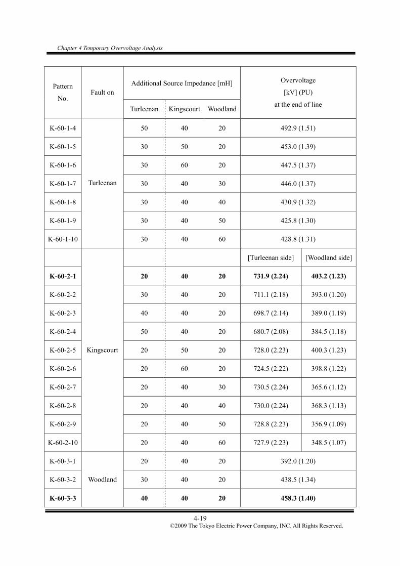
Chapter 4 Temporary Overvoltage Analysis
4-19 ©2009 The Tokyo Electric Power Company, INC. All Rights Reserved.
Additional Source Impedance [mH] Pattern
No. Fault on
Turleenan Kingscourt Woodland
Overvoltage
[kV] (PU)
at the end of line
K-60-1-4 50 40 20 492.9 (1.51)
K-60-1-5 30 50 20 453.0 (1.39)
K-60-1-6 30 60 20 447.5 (1.37)
K-60-1-7 30 40 30 446.0 (1.37)
K-60-1-8 30 40 40 430.9 (1.32)
K-60-1-9 30 40 50 425.8 (1.30)
K-60-1-10
Turleenan
30 40 60 428.8 (1.31)
[Turleenan side] [Woodland side]
K-60-2-1 20 40 20 731.9 (2.24) 403.2 (1.23)
K-60-2-2 30 40 20 711.1 (2.18) 393.0 (1.20)
K-60-2-3 40 40 20 698.7 (2.14) 389.0 (1.19)
K-60-2-4 50 40 20 680.7 (2.08) 384.5 (1.18)
K-60-2-5 20 50 20 728.0 (2.23) 400.3 (1.23)
K-60-2-6 20 60 20 724.5 (2.22) 398.8 (1.22)
K-60-2-7 20 40 30 730.5 (2.24) 365.6 (1.12)
K-60-2-8 20 40 40 730.0 (2.24) 368.3 (1.13)
K-60-2-9 20 40 50 728.8 (2.23) 356.9 (1.09)
K-60-2-10
Kingscourt
20 40 60 727.9 (2.23) 348.5 (1.07)
K-60-3-1 20 40 20 392.0 (1.20)
K-60-3-2 30 40 20 438.5 (1.34)
K-60-3-3
Woodland
40 40 20 458.3 (1.40)

Chapter 4 Temporary Overvoltage Analysis
4-20 ©2009 The Tokyo Electric Power Company, INC. All Rights Reserved.
Additional Source Impedance [mH] Pattern
No. Fault on
Turleenan Kingscourt Woodland
Overvoltage
[kV] (PU)
at the end of line
K-60-3-4 50 40 20 409.9 (1.26)
K-60-3-5 40 50 20 440.6 (1.35)
K-60-3-6 40 60 20 419.0 (1.28)
K-60-3-7 40 40 30 452.3 (1.38)
K-60-3-8 40 40 40 447.0 (1.37)
K-60-3-9 40 40 50 442.5 (1.35)
K-60-3-10
Woodland
40 40 60 438.9 (1.34)
* : 1 PU = 400kV / √3 * √2
Table 4.6 Overvoltage Caused by System Islanding (at the end of the line)
(cable ratio 60 % at Center)
Additional Source Impedance [mH] Pattern
No. Fault on
Turleenan Kingscourt Woodland
Overvoltage
[kV] (PU)
at the end of line
C-60-1-1 20 40 20 580.7 (1.78)
C-60-1-2 30 40 20 569.2 (1.74)
C-60-1-3 40 40 20 563.1 (1.72)
C-60-1-4 50 40 20 559.0 (1.71)
C-60-1-5 20 50 20 578.5 (1.77)
C-60-1-6
Turleenan
20 60 20 579.4 (1.77)

Chapter 4 Temporary Overvoltage Analysis
4-21 ©2009 The Tokyo Electric Power Company, INC. All Rights Reserved.
Additional Source Impedance [mH] Pattern
No. Fault on
Turleenan Kingscourt Woodland
Overvoltage
[kV] (PU)
at the end of line
C-60-1-7 20 40 30 565.7 (1.73)
C-60-1-8 20 40 40 552.1 (1.69)
C-60-1-9 20 40 50 543.6 (1.66)
C-60-1-10
Turleenan
20 40 60 535.6 (1.64)
[Turleenan side] [Woodland side]
C-60-2-1 20 40 20 621.3 (1.90) 407.4 (1.25)
C-60-2-2 30 40 20 585.6 (1.79) 399.5 (1.22)
C-60-2-3 40 40 20 580.3 (1.78) 394.8 (1.21)
C-60-2-4 50 40 20 601.6 (1.84) 387.2 (1.19)
C-60-2-5 60 40 20 599.2 (1.83) 389.1 (1.19)
C-60-2-6 20 50 20 617.6 (1.89) 403.7 (1.24)
C-60-2-7 20 60 20 615.1 (1.88) 402.7 (1.23)
C-60-2-8 20 40 30 619.6 (1.90) 371.0(1.14)
C-60-2-9 20 40 40 619.1 (1.90) 374.3 (1.15)
C-60-2-10 20 40 50 617.9 (1.89) 365.7 (1.12)
C-60-2-11
Kingscourt
20 40 60 617.1 (1.89) 358.8 (1.10)
C-60-3-1 20 40 20 410.1 (1.26)
C-60-3-2 30 40 20 471.6 (1.44)
C-60-3-3 40 40 20 428.7 (1.31)
C-60-3-4 50 40 20 430.1 (1.32)
C-60-3-5
Woodland
30 50 20 464.5 (1.42)

Chapter 4 Temporary Overvoltage Analysis
4-22 ©2009 The Tokyo Electric Power Company, INC. All Rights Reserved.
Additional Source Impedance [mH] Pattern
No. Fault on
Turleenan Kingscourt Woodland
Overvoltage
[kV] (PU)
at the end of line
C-60-3-6 30 60 20 450.1 (1.38)
C-60-3-7 30 40 30 466.6 (1.43)
C-60-3-8 30 40 40 462.5 (1.42)
C-60-3-9 30 40 50 460.1 (1.41)
C-60-3-10
Woodland
30 40 60 458.3 (1.40)
* : 1 PU = 400kV / √3 * √2

Chapter 4 Temporary Overvoltage Analysis
4-23 ©2009 The Tokyo Electric Power Company, INC. All Rights Reserved.
Table 4.7 Overvoltage Caused by System Islanding (at the end of the line)
(cable ratio 30 % at Kingscourt end)
Additional Source Impedance [mH] Pattern
No. Fault on
Turleenan Kingscourt Woodland
Overvoltage
[kV] (PU)
at the end of line
K-30-1-1 20 40 20 479.2 (1.47)
K-30-1-2 20 50 20 476.4 (1.46)
K-30-1-3 20 60 20 476.1 (1.46)
K-30-1-4 20 60 30 473.4 (1.45)
K-30-1-5 20 60 40 494.4 (1.51)
K-30-1-6 20 60 50 484.3 (1.48)
K-30-1-7 20 60 60 472.4 (1.45)
K-30-1-8 30 60 40 482.7 (1.48)
K-30-1-9 40 60 40 480.2 (1.47)
K-30-1-10 50 60 40 474.9 (1.45)
K-30-1-11 20 40 40
K-30-1-12
Turleenan
20 50 40 481.0 (1.47)
[Turleenan side] [Woodland side]
K-30-2-1 20 40 20 636.6 (1.95) 411.8 (1.26)
K-30-2-2 30 40 20 637.4 (1.95) 387.4 (1.19)
K-30-2-3 40 40 20 631.4 (1.93) 393.3 (1.20)
K-30-2-4 50 40 20 612.2 (1.87) 385.7 (1.18)
K-30-2-5 20 50 20 633.9 (1.94) 409.1 (1.25)
K-30-2-6
Kingscourt
20 60 20 630.8 (1.93) 408.4 (1.25)

Chapter 4 Temporary Overvoltage Analysis
4-24 ©2009 The Tokyo Electric Power Company, INC. All Rights Reserved.
Additional Source Impedance [mH] Pattern
No. Fault on
Turleenan Kingscourt Woodland
Overvoltage
[kV] (PU)
at the end of line
K-30-2-6 30 50 20 629.8 (1.93) 392.8 (1.20)
K-30-2-7 30 60 20 622.4 (1.91) 392.6 (1.20)
K-30-2-8 30 40 30 634.5 (1.94) 374.8 (1.15)
K-30-2-9 30 40 40 631.8 (1.93) 369.0 (1.13)
K-30-2-10 30 40 50 629.5 (1.93) 368.3 (1.13)
K-30-2-11
Kingscourt
20 40 60 632.9 (1.94) 372.8 (1.14)
K-30-3-1 20 40 20 454.8 (1.39)
K-30-3-2 30 40 20 487.5 (1.49)
K-30-3-3 40 40 20 480.8 (1.47)
K-30-3-4 50 40 20 467.2 (1.43)
K-30-3-5 20 50 20 450.8 (1.38)
K-30-3-6 30 50 20 495.9 (1.52)
K-30-3-7 40 50 20 475.6 (1.46)
K-30-3-8 50 50 20 430.8 (1.32)
K-30-3-9 30 60 20 487.7 (1.49)
K-30-3-10 30 50 30 487.2 (1.49)
K-30-3-11 30 50 40 481.8 (1.48)
K-30-3-12
Woodland
30 50 50 477.9 (1.46)
* : 1 PU = 400kV / √3 * √2
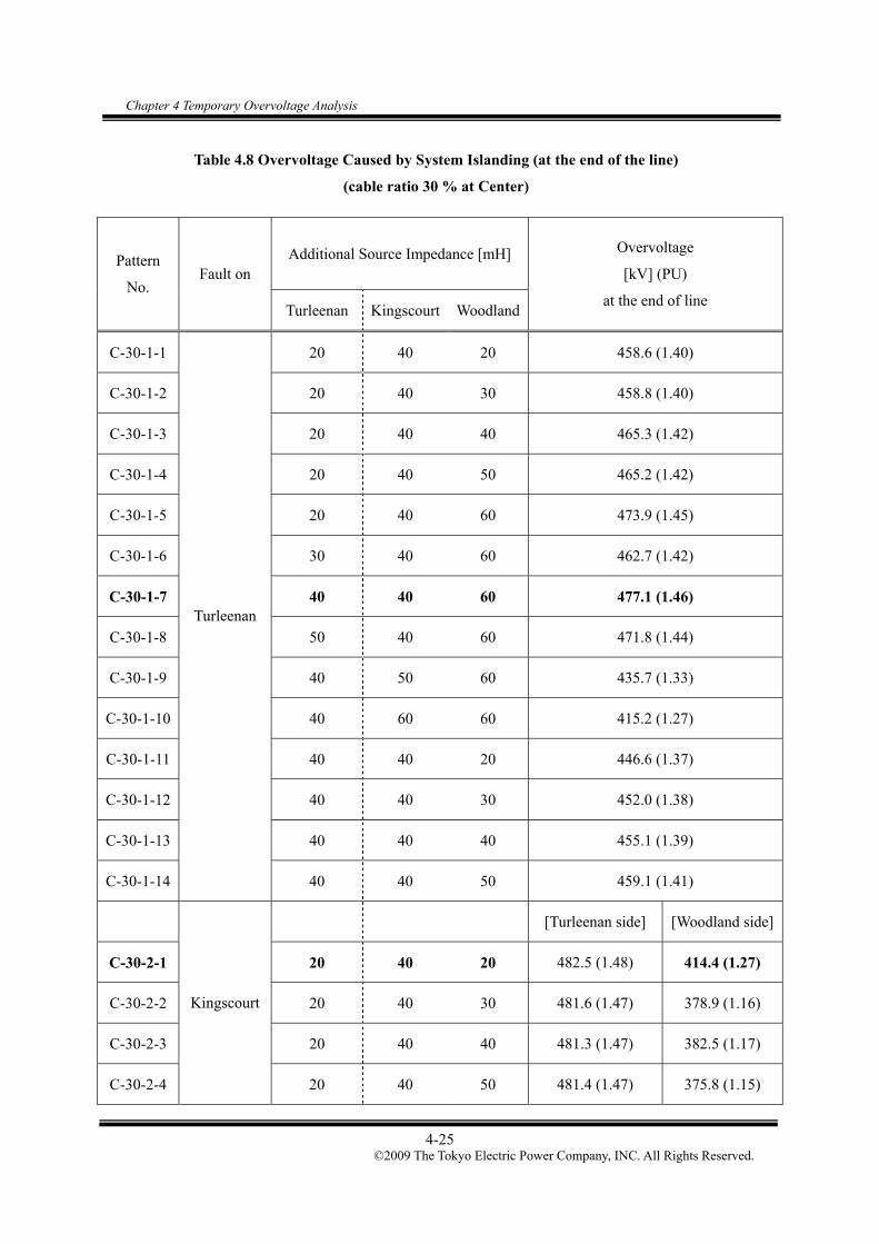
Chapter 4 Temporary Overvoltage Analysis
4-25 ©2009 The Tokyo Electric Power Company, INC. All Rights Reserved.
Table 4.8 Overvoltage Caused by System Islanding (at the end of the line)
(cable ratio 30 % at Center)
Additional Source Impedance [mH] Pattern
No. Fault on
Turleenan Kingscourt Woodland
Overvoltage
[kV] (PU)
at the end of line
C-30-1-1 20 40 20 458.6 (1.40)
C-30-1-2 20 40 30 458.8 (1.40)
C-30-1-3 20 40 40 465.3 (1.42)
C-30-1-4 20 40 50 465.2 (1.42)
C-30-1-5 20 40 60 473.9 (1.45)
C-30-1-6 30 40 60 462.7 (1.42)
C-30-1-7 40 40 60 477.1 (1.46)
C-30-1-8 50 40 60 471.8 (1.44)
C-30-1-9 40 50 60 435.7 (1.33)
C-30-1-10 40 60 60 415.2 (1.27)
C-30-1-11 40 40 20 446.6 (1.37)
C-30-1-12 40 40 30 452.0 (1.38)
C-30-1-13 40 40 40 455.1 (1.39)
C-30-1-14
Turleenan
40 40 50 459.1 (1.41)
[Turleenan side] [Woodland side]
C-30-2-1 20 40 20 482.5 (1.48) 414.4 (1.27)
C-30-2-2 20 40 30 481.6 (1.47) 378.9 (1.16)
C-30-2-3 20 40 40 481.3 (1.47) 382.5 (1.17)
C-30-2-4
Kingscourt
20 40 50 481.4 (1.47) 375.8 (1.15)

Chapter 4 Temporary Overvoltage Analysis
4-26 ©2009 The Tokyo Electric Power Company, INC. All Rights Reserved.
Additional Source Impedance [mH] Pattern
No. Fault on
Turleenan Kingscourt Woodland
Overvoltage
[kV] (PU)
at the end of line
C-30-2-5 20 40 60 481.5 (1.47) 368.9 (1.13)
C-30-2-6 20 50 20 480.1 (1.47) 412.1 (1.26)
C-30-2-7 20 60 20 479.4 (1.47) 410.5 (1.26)
C-30-2-8 30 60 20 562.3 (1.72) 402.6 (1.23)
C-30-2-9 30 60 30 591.9 (1.81) 373.7 (1.14)
C-30-2-10 30 60 40 587.4 (1.80) 378.4 (1.16)
C-30-2-11 30 60 50 583.2 (1.79) 369.5 (1.13)
C-30-2-12 30 60 60 579.9 (1.78) 364.0 (1.11)
C-30-2-13 30 40 30 571.5 (1.75) 371.9 (1.14)
C-30-2-14 30 50 30 564.4 (1.73) 368.9 (1.13)
C-30-2-15 20 60 30 478.3 (1.46) 373.8 (1.14)
C-30-2-16 40 60 30 500.3 (1.53) 376.8 (1.15)
C-30-2-17
Kingscourt
50 60 30 488.0 (1.49) 373.6 (1.14)
C-30-3-1 20 40 20 464.2 (1.42)
C-30-3-2 20 50 20 469.5 (1.44)
C-30-3-3 20 60 20 474.0 (1.45)
C-30-3-4 20 60 30 467.3 (1.43)
C-30-3-5 20 60 40 462.7 (1.42)
C-30-3-6 20 60 50 459.4 (1.41)
C-30-3-7 20 60 60 457.0 (1.40)
C-30-3-8
Woodland
30 60 20 467.1 (1.43)

Chapter 4 Temporary Overvoltage Analysis
4-27 ©2009 The Tokyo Electric Power Company, INC. All Rights Reserved.
Additional Source Impedance [mH] Pattern
No. Fault on
Turleenan Kingscourt Woodland
Overvoltage
[kV] (PU)
at the end of line
C-30-3-9 40 60 20 445.7 (1.36)
C-30-3-10
Woodland
50 60 20 459.9 (1.41)
* : 1 PU = 400kV / √3 * √2

Chapter 4 Temporary Overvoltage Analysis
4-28 ©2009 The Tokyo Electric Power Company, INC. All Rights Reserved.
The highest overvoltage at the end of the line was observed in Pattern K-60-2-1, with the fault
on Kingscourt. Fig. 4.23 shows the result of the analysis with Pattern K-60-2-1. This
overvoltage is not a concern in operation as it is damped in a few cycles.
Fig. 4.23 Overvoltage caused by system islanding in Pattern K-60-2-1.
(fi le part3 _6 0 k in g _ls _k0 1 _t2 0 k4 0 w 2 0 .p l4 ; x - va r t ) v :K IN G 4 A v :K IN G 4 B v :K IN G 4 C v :K IN G 5 A v :K IN G 5 B v :K IN G 5 C 0 .0 8 5 0 .0 9 4 0 .1 0 3 0 .1 1 2 0 .1 2 1 0 .1 3 0
- 7 5 0
- 5 0 0
- 2 5 0
0
2 5 0
5 0 0
7 5 0
* 1 0 3
(file part3_60king_ls_k01_t20k40w20.pl4; x-var t) v:KING4A v:KING4B v:KING4C v:KING5A v:KING5B v:KING5C 0.00 0.05 0.10 0.15 0.20 0.25 0.30
-750
-500
-250
0
250
500
750
*103
Turleenan side Woodland side

Chapter 4 Temporary Overvoltage Analysis
4-29 ©2009 The Tokyo Electric Power Company, INC. All Rights Reserved.
The highest overvoltage along the Turleenan – Kingscourt line in Pattern K-60-2-1 was
observed at the next point to Kingscourt. Fig. 4.24 shows the result of the maximum overvoltage
in the Turleenan – Kingscourt line in Pattern K-60-2-1.
Fig. 4.24 Overvoltage caused by system islanding in Pattern K-60-2-1 (Turleenan side).
500
550
600
650
700
750
1 2 3 4 5 6 7 8 9 10Kingscourt Turleenan
Position of Turleenan –Kingscourt line
Cable section Overhead line section
Max
imum
Ove
rvol
tage
inPa
tter
nK
-60-
2-1
(kV
) 734.0 kV (the highest)
731.9 kV

Chapter 4 Temporary Overvoltage Analysis
4-30 ©2009 The Tokyo Electric Power Company, INC. All Rights Reserved.
4.3.2 Overvoltage studies under additional conditions
The following more severe additional conditions are also studied with the overvoltage caused
by system islanding for reference. These additional cases were calculated with the three pattern of
additional equivalent source impedance, ”low pattern”, “middle pattern” and “high pattern”. The
each pattern of the source impedance is shown in Table 4.9. The highest observed overvoltage at
the end of the line in each network condition is summarized from Table 4.10 to Table 4.17.
a) Base condition (the detail study result was described in 4.3.1)
b) No load in Kingscourt substation (the switches of primary side of transformers are
opened in the initial condition)
c) The 400 kV transformers at Woodland, Kingscourt and Turleenan are tripped
together with the 400 kV cables at the same time. (shown in Fig. 4.25)
d) The 400 kV transformers at Kingscourt are disconnected from the 400 kV bus in
the initial condition as in b). In addition, the 400 kV transformers at Woodland
and Turleenan are tripped together with 400 kV cables as in c).
Note: The condition c) assumes transformers are connected to the same bus (faulted bus) as
the 400 kV cables. In contrast, in the condition a) (base condition), the 400 kV
transformers are not tripped, which assumes transformers are not connected to the
faulted bus.
In condition d), the 400 kV transformer at Kingscourt is not tripped together with 400
kV cables since it is already opened in the initial condition.
Fig. 4.25 Additional condition of transformer trip (example of a fault at the Woodland bus).
Woodland
On
MNYPG
Trip
Trip
Trip
Trip
Three-phase fault
to Kingland and Turleenan

Chapter 4 Temporary Overvoltage Analysis
4-31 ©2009 The Tokyo Electric Power Company, INC. All Rights Reserved.
Table 4.9 Overvoltage Caused by System Islanding under Additional Conditions
additional impedance (mH) source impedance
pattern Turleenan Kingscourt Woodland
low 20 40 20
middle 35 50 40
high 50 60 60
Table 4.10 Overvoltage Caused by System Islanding under Additional Conditions (Summary)
(cable ratio 60 % at Kingscourt end)
Case Source
impedance pattern
Assumed Line Outage Fault on Overvoltage
at the end of the line
K-60-a low Turleenan – Kingscourt Kingscourt – Woodland
Kingscourt 731.9 kV (2.24 pu)
[Turleenan side]
K-60-b low Turleenan – Kingscourt Kingscourt – Woodland
Kingscourt 771.0 kV (2.36 pu)
[Turleenan side]
K-60-c low Turleenan – Kingscourt Kingscourt – Woodland
Kingscourt 768.3 kV (2.35 pu)
[Turleenan side]
K-60-d low Turleenan – Kingscourt Kingscourt – Woodland
Kingscourt 771.0 kV (2.36 pu)
[Turleenan side]
* : 1 PU = 400kV / √3 * √2

Chapter 4 Temporary Overvoltage Analysis
4-32 ©2009 The Tokyo Electric Power Company, INC. All Rights Reserved.
Table 4.11 Overvoltage Caused by System Islanding under Additional Conditions (Summary)
(cable ratio 60 % at Center)
Case Source
impedance pattern
Assumed Line Outage Fault on Overvoltage
at the end of the line
C-60-a low Turleenan – Kingscourt Kingscourt – Woodland
Kingscourt 621.3 kV (1.90 pu)
[Turleenan side]
C-60-b high Turleenan – Kingscourt Kingscourt – Woodland
Kingscourt 674.0 kV (2.06 pu)
[Turleenan side]
C-60-c high Turleenan – Kingscourt Kingscourt – Woodland
Kingscourt 657.3 kV (2.01 pu)
[Turleenan side]
C-60-d low Turleenan – Kingscourt Turleenan 702.7 kV (2.15 pu)
* : 1 PU = 400kV / √3 * √2
Table 4.12 Overvoltage Caused by System Islanding under Additional Conditions (Summary)
(cable ratio 30 % at Kingscourt end)
Case Source
impedance pattern
Assumed Line Outage Fault on Overvoltage
at the end of the line
K-30-a low Turleenan – Kingscourt Kingscourt – Woodland
Kingscourt 636.6 kV (1.95 pu)
[Turleenan side]
K-30-b middle Turleenan – Kingscourt Kingscourt – Woodland
Kingscourt 683.9 kV (2.09 pu)
[Turleenan side]
K-30-c high Turleenan – Kingscourt Kingscourt – Woodland
Kingscourt 664.5 kV (2.03 pu)
[Turleenan side]
K-30-d middle Turleenan – Kingscourt Kingscourt – Woodland
Kingscourt 683.9 kV (2.09 pu)
[Turleenan side]
* : 1 PU = 400kV / √3 * √2

Chapter 4 Temporary Overvoltage Analysis
4-33 ©2009 The Tokyo Electric Power Company, INC. All Rights Reserved.
Table 4.13 Overvoltage Caused by System Islanding under Additional Conditions (Summary)
(cable ratio 30 % at Center)
Case Source
impedance pattern
Assumed Line Outage Fault on Overvoltage
at the end of the line
C-30-a middle Turleenan – Kingscourt Kingscourt – Woodland
Kingscourt 581.5 kV (1.78 pu)
[Turleenan side]
C-30-b middle Turleenan – Kingscourt Turleenan 604.1 kV (1.85 pu)
[Turleenan side]
C-30-c high Turleenan – Kingscourt Kingscourt – Woodland
Kingscourt 644.1 kV (1.97 pu)
[Turleenan side]
C-30-d middle Turleenan – Kingscourt Turleenan 647.9 kV (1.98 pu)
* : 1 PU = 400kV / √3 * √2
Table 4.14 Overvoltage Caused by System Islanding under Additional Conditions
(cable ratio 60 % at Kingscourt end)
Case Source
impedance pattern
Assumed Line Outage Fault on
Overvoltage
[kV] (pu)
at the end of line
low 459.3 (1.41)
middle 425.2 (1.30)
high
Turleenan – Kingscourt Turleenan
425.0 (1.30)
[Turleenan side] [Woodland side]
low 731.9 (2.24) 403.2 (1.23)
middle 696.2 (2.13) 353.3 (1.08)
high
Turleenan – Kingscourt Kingscourt – Woodland
Kingscourt
658.9 (2.02) 347.5 (1.06)
low 392.0 (1.20)
middle 448.0 (1.37)
K-60-a
high
Kingscourt – Woodland Woodland
448.7 (1.37)
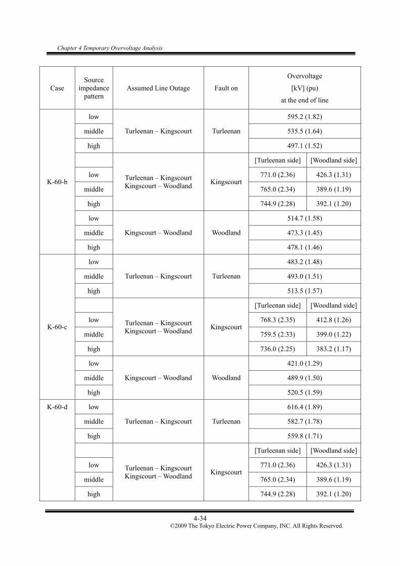
Chapter 4 Temporary Overvoltage Analysis
4-34 ©2009 The Tokyo Electric Power Company, INC. All Rights Reserved.
Case Source
impedance pattern
Assumed Line Outage Fault on
Overvoltage
[kV] (pu)
at the end of line
low 595.2 (1.82)
middle 535.5 (1.64)
high
Turleenan – Kingscourt Turleenan
497.1 (1.52)
[Turleenan side] [Woodland side]
low 771.0 (2.36) 426.3 (1.31)
middle 765.0 (2.34) 389.6 (1.19)
high
Turleenan – Kingscourt Kingscourt – Woodland
Kingscourt
744.9 (2.28) 392.1 (1.20)
low 514.7 (1.58)
middle 473.3 (1.45)
K-60-b
high
Kingscourt – Woodland Woodland
478.1 (1.46)
low 483.2 (1.48)
middle 493.0 (1.51)
high
Turleenan – Kingscourt Turleenan
513.5 (1.57)
[Turleenan side] [Woodland side]
low 768.3 (2.35) 412.8 (1.26)
middle 759.5 (2.33) 399.0 (1.22)
high
Turleenan – Kingscourt Kingscourt – Woodland
Kingscourt
736.0 (2.25) 383.2 (1.17)
low 421.0 (1.29)
middle 489.9 (1.50)
K-60-c
high
Kingscourt – Woodland Woodland
520.5 (1.59)
low 616.4 (1.89)
middle 582.7 (1.78)
high
Turleenan – Kingscourt Turleenan
559.8 (1.71)
[Turleenan side] [Woodland side]
low 771.0 (2.36) 426.3 (1.31)
middle 765.0 (2.34) 389.6 (1.19)
K-60-d
high
Turleenan – Kingscourt Kingscourt – Woodland
Kingscourt
744.9 (2.28) 392.1 (1.20)

Chapter 4 Temporary Overvoltage Analysis
4-35 ©2009 The Tokyo Electric Power Company, INC. All Rights Reserved.
Case Source
impedance pattern
Assumed Line Outage Fault on
Overvoltage
[kV] (pu)
at the end of line
low 551.7 (1.69)
middle 526.7 (1.61)
high
Kingscourt – Woodland Woodland
565.4 (1.73)
Table 4.15 Overvoltage Caused by System Islanding under Additional Conditions
(cable ratio 60 % at Center)
Case Source
impedance pattern
Assumed Line Outage Fault on
Overvoltage
[kV] (pu)
at the end of line
low 580.7 (1.78)
middle 532.2 (1.63)
high
Turleenan – Kingscourt Turleenan
495.3 (1.52)
[Turleenan side] [Woodland side]
low 621.3 (1.90) 407.4 (1.25)
middle 570.7 (1.75) 360.9 (1.11)
high
Turleenan – Kingscourt Kingscourt – Woodland
Kingscourt
587.4 (1.80) 346.6 (1.06)
low 410.1 (1.26)
middle 426.5 (1.31)
C-60-a
high
Kingscourt – Woodland Woodland
424.5 (1.30)
low 666.8 (2.04)
middle 607.5 (1.86)
high
Turleenan – Kingscourt Turleenan
560.6 (1.72)
[Turleenan side] [Woodland side]
low 658.1 (2.02) 431.3 (1.32)
middle 628.4 (1.92) 396.9 (1.22)
C-60-b
high
Turleenan – Kingscourt Kingscourt – Woodland
Kingscourt
674.0 (2.06) 376.6 (1.15)

Chapter 4 Temporary Overvoltage Analysis
4-36 ©2009 The Tokyo Electric Power Company, INC. All Rights Reserved.
Case Source
impedance pattern
Assumed Line Outage Fault on
Overvoltage
[kV] (pu)
at the end of line
low 455.0 (1.39)
middle 483.7 (1.48)
high
Kingscourt – Woodland Woodland
433.7 (1.33)
low 631.6 (1.93)
middle 615.3 (1.88)
high
Turleenan – Kingscourt Turleenan
609.0 (1.86)
[Turleenan side] [Woodland side]
low 653.4 (2.00) 416.3 (1.27)
middle 614.9 (1.88) 401.4 (1.23)
high
Turleenan – Kingscourt Kingscourt – Woodland
Kingscourt
657.3 (2.01) 384.6 (1.18)
low 425.7 (1.30)
middle 471.1 (1.44)
C-60-c
high
Kingscourt – Woodland Woodland
504.7 (1.55)
low 702.7 (2.15)
middle 662.8 (2.03)
high
Turleenan – Kingscourt Turleenan
623.4 (1.91)
[Turleenan side] [Woodland side]
low 658.1 (2.02) 431.3 (1.32)
middle 628.4 (1.92) 396.9 (1.22)
high
Turleenan – Kingscourt Kingscourt – Woodland
Kingscourt
674.0 (2.06) 376.6 (1.15)
low 490.1 (1.50)
middle 539.5 (1.65)
C-60-d
high
Kingscourt – Woodland Woodland
497.9 (1.52)

Chapter 4 Temporary Overvoltage Analysis
4-37 ©2009 The Tokyo Electric Power Company, INC. All Rights Reserved.
Table 4.16 Overvoltage Caused by System Islanding under Additional Conditions
(cable ratio 30 % at Kingscourt end)
Case Source
impedance pattern
Assumed Line Outage Fault on
Overvoltage
[kV] (pu)
at the end of line
low 479.2 (1.47)
middle 480.2 (1.47)
high
Turleenan – Kingscourt Turleenan
442.4 (1.35)
[Turleenan side] [Woodland side]
low 636.6 (1.95) 411.8 (1.26)
middle 618.3 (1.89) 373.2 (1.14)
high
Turleenan – Kingscourt Kingscourt – Woodland
Kingscourt
589.5 (1.80) 352.8 (1.08)
low 454.8 (1.39)
middle 470.3 (1.44)
K-30-a
high
Kingscourt – Woodland Woodland
421.9 (1.29)
low 537.6 (1.65)
middle 498.9 (1.53)
high
Turleenan – Kingscourt Turleenan
414.5 (1.27)
[Turleenan side] [Woodland side]
low 677.2 (2.07) 445.6 (1.36)
middle 683.9 (2.09) 401.8 (1.23)
high
Turleenan – Kingscourt Kingscourt – Woodland
Kingscourt
675.8 (2.07) 417.1 (1.28)
low 469.8 (1.44)
middle 477.7 (1.46)
K-30-b
high
Kingscourt – Woodland Woodland
469.7 (1.44)
low 507.0 (1.55)
middle 522.4 (1.60)
K-30-c
high
Turleenan – Kingscourt Turleenan
513.9 (1.57)

Chapter 4 Temporary Overvoltage Analysis
4-38 ©2009 The Tokyo Electric Power Company, INC. All Rights Reserved.
Case Source
impedance pattern
Assumed Line Outage Fault on
Overvoltage
[kV] (pu)
at the end of line
[Turleenan side] [Woodland side]
low 664.4 (2.03) 419.0 (1.28)
middle 664.2 (2.03) 423.5 (1.30)
high
Turleenan – Kingscourt Kingscourt – Woodland
Kingscourt
664.5 (2.03) 394.8 (1.21)
low 491.1 (1.50)
middle 526.4 (1.61)
high
Kingscourt – Woodland Woodland
489.9 (1.50)
low 555.0 (1.70)
middle 479.1 (1.47)
high
Turleenan – Kingscourt Turleenan
488.1 (1.49)
[Turleenan side] [Woodland side]
low 677.2 (2.07) 445.6 (1.36)
middle 683.9 (2.09) 401.8 (1.23)
high
Turleenan – Kingscourt Kingscourt – Woodland
Kingscourt
675.8 (2.07) 417.1 (1.28)
low 503.0 (1.54)
middle 530.7 (1.62)
K-30-d
high
Kingscourt – Woodland Woodland
552.9 (1.69)
Table 4.17 Overvoltage Caused by System Islanding under Additional Conditions
(cable ratio 30 % at Center)
Case Source
impedance pattern
Assumed Line Outage Fault on
Overvoltage
[kV] (pu)
at the end of line
low 458.6 (1.40)
middle 464.3 (1.42)
C-30-a
high
Turleenan – Kingscourt Turleenan
409.7 (1.25)

Chapter 4 Temporary Overvoltage Analysis
4-39 ©2009 The Tokyo Electric Power Company, INC. All Rights Reserved.
Case Source
impedance pattern
Assumed Line Outage Fault on
Overvoltage
[kV] (pu)
at the end of line
[Turleenan side] [Woodland side]
low 482.5 (1.48) 414.4 (1.27)
middle 581.5 (1.78) 375.6 (1.15)
high
Turleenan – Kingscourt Kingscourt – Woodland
Kingscourt
574.7 (1.76) 358.6 (1.10)
low 464.2 (1.42)
middle 408.3 (1.25)
high
Kingscourt – Woodland Woodland
428.2 (1.31)
low 569.3 (1.74)
middle 604.1 (1.85)
high
Turleenan – Kingscourt Turleenan
530.3 (1.62)
[Turleenan side] [Woodland side]
low 506.2 (1.55) 439.9 (1.35)
middle 557.6 (1.71) 401.3 (1.23)
high
Turleenan – Kingscourt Kingscourt – Woodland
Kingscourt
558.5 (1.71) 387.3 (1.19)
low 470.6 (1.44)
middle 466.1 (1.43)
C-30-b
high
Kingscourt – Woodland Woodland
426.8 (1.31)
low 504.8 (1.55)
middle 530.7 (1.62)
high
Turleenan – Kingscourt Turleenan
520.6 (1.59)
[Turleenan side] [Woodland side]
low 508.3 (1.56) 422.9 (1.29)
middle 641.4 (1.96) 418.7 (1.28)
high
Turleenan – Kingscourt Kingscourt – Woodland
Kingscourt
644.1 (1.97) 407.0 (1.25)
low 506.1 (1.55)
middle 459.1 (1.41)
C-30-c
high
Kingscourt – Woodland Woodland
488.5 (1.50)

Chapter 4 Temporary Overvoltage Analysis
4-40 ©2009 The Tokyo Electric Power Company, INC. All Rights Reserved.
Case Source
impedance pattern
Assumed Line Outage Fault on
Overvoltage
[kV] (pu)
at the end of line
low 581.3 (1.78)
middle 647.9 (1.98)
high
Turleenan – Kingscourt Turleenan
589.0 (1.80)
[Turleenan side] [Woodland side]
low 506.2 (1.55) 439.9 (1.35)
middle 557.6 (1.71) 401.3 (1.23)
high
Turleenan – Kingscourt Kingscourt – Woodland
Kingscourt
558.5 (1.71) 387.3 (1.19)
low 501.4 (1.54)
middle 518.1 (1.59)
C-30-d
high
Kingscourt – Woodland Woodland
488.5 (1.50)

Chapter 4 Temporary Overvoltage Analysis
4-41 ©2009 The Tokyo Electric Power Company, INC. All Rights Reserved.
The highest overvoltage at the end of the line was observed in case K-60-b (and K-60-d) and
low impedance pattern, with the fault on Kingscourt. Fig. 4.26 shows the result of the analysis in
this case. This overvoltage is not a concern in operation because it is damped in a few cycles and
it can be evaluated by SIWV (1050 kV) due to its rapid decaying properties.
Fig. 4.26 Overvoltage caused by system islanding in case K-60-b and low impedance pattern.
(file part3_60king_ls_k01_t20k40w20_1m.pl4; x-var t) v:KING4A v:KING4B v:KING4C 0.085 0.095 0.105 0.115 0.125 0.135 0.145 0.155
-800
-500
-200
100
400
700
*103
(file part3_60king_ls_k01_t20k40w20_1m.pl4; x-var t) v:KING4A v:KING4B v:KING4C 0.0 0.2 0.4 0.6 0.8 1.0
-800
-500
-200
100
400
700
*10 3
771.0kV

Chapter 4 Temporary Overvoltage Analysis
4-42 ©2009 The Tokyo Electric Power Company, INC. All Rights Reserved.
4.4 Conclusion
The temporary overvoltage analysis was performed based on the compensation pattern
determined by the reactive power compensation analysis. Resonance overvoltage and overvoltage
caused by load shedding were studied under different network conditions.
No significant overvoltage was found in the parallel resonance overvoltage analysis. As in
Part 1 and 2 studies, load sheddings yielded very high overvoltages, but this is not a concern for the
safe operation of the network as it can be evaluated by SIWV (1050 kV) due to its rapid decaying
properties.
Table 4-18 Summary of the Temporary Overvoltage Analysis
Highest overvoltage
(peak)
Withstand voltage
for evaluation
Parallel resonance 500.5 kV (1.53 pu) 370 kV (r.m.s.)
(1.60 pu) for 10 seconds
Load shedding 771.0 kV (2.36 pu) 1050 kV (peak)
(r.m.s.) 3
1kV 220or 400 (peak),
3
2kV 220or 400pu 1

Chapter 5 Overvoltage Caused by Autoreclose
5-1 ©2009 The Tokyo Electric Power Company, INC. All Rights Reserved.
Chapter 5 Overvoltage Caused by Autoreclose
When single phase autoreclose is applied to a mixed OHL / underground cable, it is necessary
to study the overvoltage caused by autoreclose. The conditions for single phase autoreclose are
different from line energisation at the following points:
(1) The cable is re-energised before the cable is discharged, and
(2) Only the faulted phase is opened and re-energised.
Here, the condition (1) is true when a shunt reactor is directly connected to the line. When a
shunt reactor is not connected to the line, the cable will be discharged through the VTs, not through
the shunt reactors. In such a case, cable discharge is completed before the line is re-energised.
The overvoltage caused by single phase autoreclose can be higher than the overvoltage caused
by line energisation because of condition (1). For example, if the faulted phase has a negative
residual voltage of -1.0 pu, a sudden voltage rise of 2.0 pu (from -1.0 pu to 1.0 pu) can be caused in
the faulted phase when the cable is re-energised from the bus whose voltage is 1.0 pu. In order to
yield a severe condition:
Timing of re-energisation has to be adjusted so that re-energisation occurs at the most
severe timing, and
Resistance of shunt reactors has to be small enough to have large residual voltage
However, at the same time, the overvoltage caused by autoreclose may be lower than the
overvoltage caused by line energisation. This is because circuit breakers on both sides of the line
are reclosed simultaneously. There is no open end terminal (total positive reflection point) after
autoreclose even though there can be a few milliseconds time difference.
5.1 Simulation conditions
Overvoltage caused by single phase autoreclose was studied by switching scenarios shown in
Fig. 5-1. Statistical analysis was not applied since the timing of re-energisation was adjusted to
the most severe timing. In addition, it is not necessary to consider the close timing difference
between these phases since only one faulted phase will be re-energised. Note that the surge
arrester is not considered in the simulations.

Chapter 5 Overvoltage Caused by Autoreclose
5-2 ©2009 The Tokyo Electric Power Company, INC. All Rights Reserved.
Fig. 5-1 Switching scenario for the overvoltage caused by autoreclose.
The simulations were performed under conditions in which 30 % or 60 % 400 kV 2 cct cables
existed in the centre of the Turleenan – Kingscourt line. For the 60 % cable case, different
locations of for the 400 kV shut reactors were also considered.
Case 1 - 30% 400kV cable in centre
Case 2 - 60% 400kV cable in centre and 400 kV reactors at the line ends
Woodland Kingscourt
OHL 1 cct
58 km
Cable 2 cct
OHL 1 cct
49.2 km(60 %)
16.4 km(20 %)
200 MVA × 2 200 MVA × 2
OHL 1 cct
16.4 km(20 %)
Turleenan
Case 3 - 60% 400kV cable in centre and 400 kV reactors at the cable ends
Fig. 5-2 System configuration of the simulations.

Chapter 5 Overvoltage Caused by Autoreclose
5-3 ©2009 The Tokyo Electric Power Company, INC. All Rights Reserved.
Table 5-1 Standard auto-reclose sequence
Step Time Description
Step 0 0 (ms) Single phase fault (Phase A) on overhead line section near Kingscourt
Step 1 60 (ms) Tripping CB (Phase A) of both sides
Step 2 60 + (ms) Fault clearing after tripping CB
Step 3 960 (ms) Reclosing CB (Phase A) of both ends
Table 5-1 shows the standard sequence of autoreclose. As described in the Part 2 study,
the ground fault near Kingscourt yielded the largest overvoltage due to its large current through
circuit breaker. Hence, a ground fault in the overhead line section near Kingscourt was assumed
in this study.
5.2 Residual Voltage in Typical Operation
Fig. 5-3 illustrates the residual voltage in Phase A (faulted phase) which was observed at
Kingscourt in each case using the standard autoreclose sequence mentioned above. As the line
was fully compensated by shunt reactors directly connected to the cable, the waveform of voltage at
the Turleenan side was almost equal to the Kingscourt side, and it contained two frequency
components.
The peak residual voltages were observed during the first or second oscillatory voltage after
the fault clearing. The residual voltages decayed gradually through the shunt reactors on the cable,
and the voltage at the reclosing timing became 2/3 of the one at the fault clearing. The maximum
and minimum residual voltages were recorded in Cases 1 and 3 respectively, but the difference
between them was minute as shown in Fig. 5-3.

Chapter 5 Overvoltage Caused by Autoreclose
5-4 ©2009 The Tokyo Electric Power Company, INC. All Rights Reserved.
Fig. 5-3 Residual voltage in Phase A at Kingscourt in the standard operation.
(file part3_30centre_961ms.pl4; x-var t) v:SW021A 0.0 0.2 0.4 0.6 0.8 1.0 1.2[s]
-500
-375
-250
-125
0
125
250
375
500
[kV] Case 1
Fault clearing Reclose
(file part3_60centre_961ms.pl4; x-var t) v:SW021A 0.0 0.2 0.4 0.6 0.8 1.0 1.2[s]
-500
-375
-250
-125
0
125
250
375
500
[kV] Case 2
Fault clearing Reclose
(file part3_60centre_shr_961ms.pl4; x-var t) v:SW021A 0.0 0.2 0.4 0.6 0.8 1.0 1.2[s]
-500
-375
-250
-125
0
125
250
375
500
[kV] Case 3
Fault clearing Reclose
Peak period of oscillatory residual voltage
Peak period of oscillatory residual voltage
Peak period of oscillatory residual voltage

Chapter 5 Overvoltage Caused by Autoreclose
5-5 ©2009 The Tokyo Electric Power Company, INC. All Rights Reserved.
5.3 Effect of Fault Clearing Timing on Residual Voltage
According to the NIE/EirGrid standard, the fault is cleared within 60 ms as shown in Table
5-1. During the actual power system operation, the fault is sometimes cleared earlier than 60 ms.
Fig. 5-4 shows the current through circuit breakers of Kingscourt and Turleenan in Case 1. As can
be seen from the figure, both circuits have 6-times of zero crossing points within 60 ms.
Fig. 5-4 Current through circuit breakers of Kingscourt and Turleenan.
In order to understand the effect of fault clearing timing on residual voltage, different fault
clearing timings were studied as shown in Fig. 5-5 and Table 5-2. The figure shows the
waveforms of residual voltage on the cable with different fault clearing timings.
It can be seen that the maximum residual voltage was observed when the fault was cleared at
the first zero crossing. This is a typical result since a large amount of the surge components of the
ground fault are included at the 1st and/or 2nd zero crossing periods and it decays fast. In order to
consider severe overvoltage, this study assumed the fault clearing at the first zero crossing on the
faulted phase and then the reclosing at the most severe timing before 900 ms.
(file Part3 30Centre xxms 50ms 1100ms.pl4; x-var t) c:KING4A-SW021A c:SW011A-TURL4A 0 10 20 30 40 50 60 70[ms]
-6000
-4000
-2000
0
2000
4000
[A] Kingscourt
Turleenan
1st zero crossing
2nd zero crossing
3rd zero crossing
4th zero crossing
5th zero crossing
6th zero crossing
Fault 1(ms)

Chapter 5 Overvoltage Caused by Autoreclose
5-6 ©2009 The Tokyo Electric Power Company, INC. All Rights Reserved.
Fig. 5-5 Residual voltages by different fault clearing timings.
Table 5-2 Peak residual voltage for each fault clearing timing.
Fault clearing timings Peak residual voltage
1st zero crossing 335 (kV)
2nd zero crossing 175 (kV)
3rd zero crossing 143 (kV)
4th zero crossing 131 (kV)
5th zero crossing 107 (kV)
6th zero crossing 104 (kV)
0.00 0.05 0.10 0.15 0.20 0.25 0.30[s]
-400
-300
-200
-100
0
100
200
300
400
[kV]1st zero crossing
2nd zero crossing
3rd zero crossing
4th zero crossing
5th zero crossing
6th zero crossing

Chapter 5 Overvoltage Caused by Autoreclose
5-7 ©2009 The Tokyo Electric Power Company, INC. All Rights Reserved.
5.4 Reclosing Timing
In general, the switching overvoltage becomes large when the voltage difference between
the two contacts of the circuit breaker (the system voltage at the bus against the residual voltage on
the cable) is large. As shown in Fig. 5-3, the residual voltage becomes oscillatory waveform by
combination of cable capacitance and inductance of shut reactor, and it decays with time.
Fig. 5-6 illustrates the voltage between the circuit breaker contacts after the fault clearing.
The peak voltage between the circuit breaker contacts appears periodically. In this study, it was
assumed that the line was reclosed at the second peak voltage between the circuit breaker contacts.
This assumption was made in order to cause higher overvoltage, but it is not a realistic assumption
since the line is reclosed 900 ms after the fault clearing in the actual operation according to the
standard sequence.
Fig. 5-6 Voltage between circuit breaker contacts
(file Part3_30Centre_230ms_1ms_400ms_report.pl4; x-var t) v:KING4A-SW021A v:KING4A v:SW021A
0.05 0.10 0.15 0.20 0.25 0.30 0.35 0.40[s]-500
-375
-250
-125
0
125
250
375
500
[kV]Voltage between contacts
System voltage
Residual voltage on cable
Peak voltage between contacts
Peak voltage between contacts
Peak voltage between contacts
Peak voltage between contacts
Peak voltage between contacts
Peak voltage between contacts

Chapter 5 Overvoltage Caused by Autoreclose
5-8 ©2009 The Tokyo Electric Power Company, INC. All Rights Reserved.
5.5 Simulation Results
The following table and figures show the simulation results. The maximum overvoltage at
each case was observed at Turleenan, but the waveforms of all the nodes along the cable line were
approximately equal, as the 400 kV cables were compensated to around 100 %.
The maximum reclosing overvoltage was 523 kV in Case 3. The overvoltage of 1.61 pu (=
523 kV) is far below SIWV of the 400 kV cable even without surge arresters. The amount of the
cable and the location of the shunt reactors did not significantly impact the overvoltage.
Table 5-3 Simulated results
Items Case 1 Case 2 Case 3
Cable amount 30% (centre) 60% (centre) 60% (centre)
Shut reactor location Line ends Line ends Cable ends
Difference between circuit breaker contacts at reclosing (Kingscourt bus voltage and cable residual voltage)
463 (kV) 418 (kV) 445 (kV)
Maximum reclosing overvoltage 467 (kV) 505 (kV) 523 (kV)
Observed at Turleenan Turleenan Turleenan

Chapter 5 Overvoltage Caused by Autoreclose
5-9 ©2009 The Tokyo Electric Power Company, INC. All Rights Reserved.
Waveform of the cable end at Turleenan
Fig. 5-7 Reclosing waveform at Turleenan – 30 % cable.
(file Part3_30Centre_wto_FF_230ms_1ms_400ms.pl4; x-var t) v:SW011A v:SW011B v:SW011C
0.00 0.05 0.10 0.15 0.20 0.25 0.30 0.35 0.40[s]-500
-375
-250
-125
0
125
250
375
500
[kV]
467(kV)
(file Part3_30Centre_wto_FF_230ms_1ms_400ms.pl4; x-var t) v:TURL4A v:SW011A v:SW011A-TURL4A
0.00 0.05 0.10 0.15 0.20 0.25 0.30 0.35 0.40[s]-600
-400
-200
0
200
400
600
[kV]
467(kV)
Reclose of Phase A (Reclosed at maximum voltage difference timing)
Reclose of Phase A
Ground fault at OHL near Kingscourt Phase A (1ms)
Fault clearing of Phase A
Phase A
Phase B
Phase C
Turleenan cable end Turleenan bus Voltage between circuit breaker contacts at Turleenan

Chapter 5 Overvoltage Caused by Autoreclose
5-10 ©2009 The Tokyo Electric Power Company, INC. All Rights Reserved.
Waveform of the cable end at Turleenan
Fig. 5-8 Reclosing waveform at Turleenan - 30% cable, reactors at line ends. (file Part3_60Centre_wto_FF_219.3ms_1ms_400ms.pl4; x-var t) v:TURL4A v:SW011A v:SW011A-TURL4A
0.00 0.05 0.10 0.15 0.20 0.25 0.30 0.35 0.40[s]-600
-400
-200
0
200
400
600
[kV]
(file Part3_60Centre_wto_FF_219.3ms_1ms_400ms.pl4; x-var t) v:SW011A v:SW011B v:SW011C
0.00 0.05 0.10 0.15 0.20 0.25 0.30 0.35 0.40[s]-500
-280
-60
160
380
600
[kV]505 (kV)
Phase A
Phase B
Phase C
Reclose of Phase A
Ground fault at OHL near Kingscourt Phase A (1ms)
Fault clearing of Phase A
Reclose of Phase A (Reclosed at maximum voltage difference timing)
505 (kV)
Turleenan cable end Turleenan bus Voltage between circuit breaker contacts at Turleenan
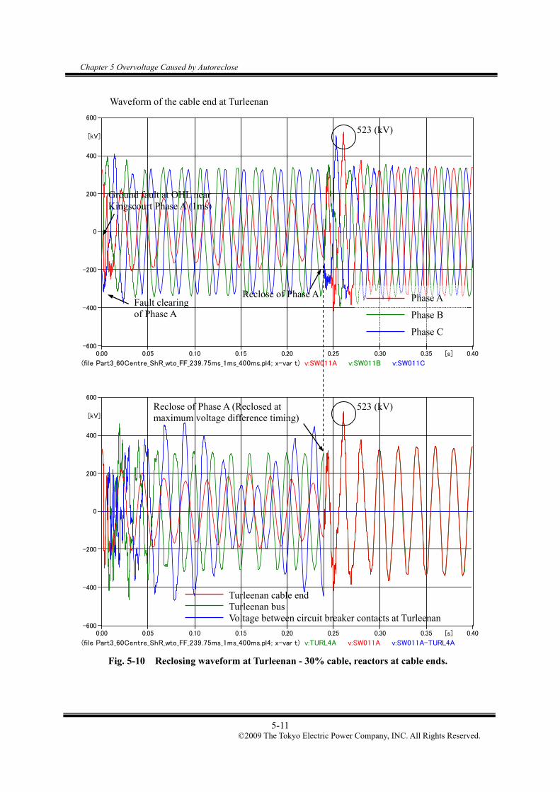
Chapter 5 Overvoltage Caused by Autoreclose
5-11 ©2009 The Tokyo Electric Power Company, INC. All Rights Reserved.
Waveform of the cable end at Turleenan
Fig. 5-9 Waveform of reclose at fault point (Kingscourt) - 60% cable, ShR at cable ends.
Fig. 5-10 Reclosing waveform at Turleenan - 30% cable, reactors at cable ends.
(file Part3_60Centre_ShR_wto_FF_239.75ms_1ms_400ms.pl4; x-var t) v:SW011A v:SW011B v:SW011C
0.00 0.05 0.10 0.15 0.20 0.25 0.30 0.35 0.40[s]-600
-400
-200
0
200
400
600
[kV]
(file Part3_60Centre_ShR_wto_FF_239.75ms_1ms_400ms.pl4; x-var t) v:TURL4A v:SW011A v:SW011A-TURL4A
0.00 0.05 0.10 0.15 0.20 0.25 0.30 0.35 0.40[s]-600
-400
-200
0
200
400
600
[kV]
523 (kV)
Reclose of Phase A
Ground fault at OHL near Kingscourt Phase A (1ms)
Fault clearing of Phase A
Phase A
Phase B
Phase C
523 (kV)
Turleenan cable end Turleenan bus Voltage between circuit breaker contacts at Turleenan
Reclose of Phase A (Reclosed at maximum voltage difference timing)

Chapter 5 Overvoltage Caused by Autoreclose
5-12 ©2009 The Tokyo Electric Power Company, INC. All Rights Reserved.
5.6 Three Phase Autoreclose
It may be necessary for the NIE/EirGrid to achieve a reactive power compensation rate closer
to 100 % in order to control the voltage profile and reactive power flow in the network and to
prevent harmful overvoltages. It was discussed in Section 2.3 that one of the following two
countermeasures had to be taken in order to achieve compensation rate of 100 %:
Adoption of four-legged reactors
Adoption of three phase autoreclose
The reliability of the interconnector is undermined by the adoption of three phase autoreclose,
but open phase resonance does not occur since all three phases are opened even in single line to
ground faults.
The overvoltage caused by three phase autoreclose was studied in this section since the
condition becomes more severe compared to single phase autoreclose. Statistical analysis should
be considered in the three phase autoreclose analysis, as six phases of the circuit breakers at both
ends are closed all together with only a few seconds time difference in between. The same fault
conditions and randomness as the Part 2 study was adopted.
Fig. 5-11 shows the system condition of the simulation, which is the same as the one in Case 3
shown in Fig. 5-2 which produced the maximum overvoltage in the single phase autoreclose
analysis discussed in previous sections. In this scenario, the fault occurred at the Kingscourt –
Turleenan line near Kingscourt, and it was cleared by opening CBs (three phases) at Kingscourt
and Turleenan.
Woodland Kingscourt
OHL 1 cct
58 km
Cable 2 cct
OHL 1 cct
49.2 km(60 %)
16.4 km(20 %)
200 MVA × 2 200 MVA × 2
OHL 1 cct
16.4 km(20 %)
Turleenan
Case 3 - 60% 400kV cable in center position and 400kV ShR at the cable ends
Fig. 5-11 System configuration of three phase autoreclose simulation.
The simulation results are shown in Fig. 5-12 and Fig. 5-13. The maximum overvoltage, 631
kV, was observed at Turleenan, which is higher than the single phase autoreclose (523 kV) due to
consideration of switch timing difference between each phase of both circuit breakers. However,
even after taking into consideration the switch timing difference between the phases, the maximum
overvoltage is still far below SIWV even without surge arrestors. The simulation did not identify

Chapter 5 Overvoltage Caused by Autoreclose
5-13 ©2009 The Tokyo Electric Power Company, INC. All Rights Reserved.
the obvious overvoltage difference between the nodes of overhead line sections and the cable
section.

Chapter 5 Overvoltage Caused by Autoreclose
5-14 ©2009 The Tokyo Electric Power Company, INC. All Rights Reserved.
Fig. 5-12 Voltage profile in three phase auto-reclose analysis.
Reclose timing Phase A Phase B Phase C
Turleenan 248.032 ms 245.822 ms 246.606 ms
Kingscourt 247.090 ms 245.735 ms 245.914 ms
Fig. 5-13 Waveform of maximum overvoltage (Turleenan bus).
1.94 1.85 1.83 1.85 1.84 1.84 1.83 1.82 1.80 1.78 1.78 1.81 1.82 1.84 1.84 1.89
1.84 1.77 1.76 1.77 1.78 1.78 1.77 1.77 1.75 1.73 1.73 1.74 1.73 1.74 1.74 1.74
0.0
0.5
1.0
1.5
2.0
2.5
3.0
3.5
Turleenan
KT
18
KT
17
KT
14
KT
11
KT
08
KT
05
KT
02
KT
01
Kingscourt
WK
05
WK
04
WK
03
WK
02
WK
01
Woodland
(pu)
Maximum
2%
Switching Impulse Withstand Overvoltage 1050kV (3.21pu)
Cable
(file Part3_60Centre_ShR_wto_FF_240_1ms_400ms_3phase_max.pl4; x-var t) v:TURL1A v:TURL1B v:TURL1C
0.00 0.05 0.10 0.15 0.20 0.25 0.30 0.35[s]-700
-525
-350
-175
0
175
350
525
700
[kV] Turleenan bus voltage
Phase A Phase B Phase C
631kV
Phase A ground fault at Kingscourt
Fault clearing by opening 3 phases
Reclosing
)kV 3
2400pu1(

Chapter 5 Overvoltage Caused by Autoreclose
5-15 ©2009 The Tokyo Electric Power Company, INC. All Rights Reserved.
5.7 Conclusion
The analysis did not find significant overvoltage caused by autorelose. The observed
overvoltages were much lower than SIWV in all simulated cases.
Table 5-4 Summary of the Overvoltage Caused by Autoreclose
Highest overvoltage
(peak)
Withstand voltage (peak)
for evaluation
Single phase autoreclose 523.0 kV (1.60 pu)
Three phase autoreclose 631.0 kV (1.93 pu) 1050 kV
(peak) 3
2kV 400pu 1

Chapter 6 Lightning Overvoltage
6-1 ©2009 The Tokyo Electric Power Company, INC. All Rights Reserved.
Chapter 6 Lightning Overvoltage
6.1 Overview
In Chapter 6, the lightning overvoltage analysis was performed in order to evaluate the
overvoltage in the metallic sheath. When a lightning strikes the ground wire near the connection
between OHL and the underground cable as shown in Fig. 6.1, lightning current that flows into
earth through the gantry may cause a very high overvoltage in the metallic sheath.
Fig. 6.1 Lightning overvoltage in metallic sheath.
As can be seen from Fig. 6.1, the level of the overvoltage highly depends on footing resistance
of the gantry. When a very high overvoltage is observed in the metallic sheath, it is necessary to
evaluate the energy absorption capability of the SVLs.

Chapter 6 Lightning Overvoltage
6-2 ©2009 The Tokyo Electric Power Company, INC. All Rights Reserved.
6.2 Model Setup
The main focus of the lightning overvoltage analysis is the connection between the OHL and
the underground cable. Hence, the simulation model near the point of interest has to be more
detailed compared to other analyses. On the other hand, equipment far from the point of interest
can be excluded from the simulation model. This section discusses only the differences of the
simulation model used for the lightning overvoltage analysis from the model for other analyses.
Z2Z2
Z1
XX0011
TW2G
10 ohm
Z2
Z1
XX0010
TW1G
10 ohm
Z2
Z1
XX0012
TW3G
Z2
10 ohm
Z2Z2
Z1
XX0013
TW4G
10 ohm
Z2Z2
Z1
XX0014
TW5G
10 ohm
Z2TW1T2 TW1T1TW2T2 TW2T1TW3T2 TW3T1TW4T2 TW4T1TW5T2 TW5T1
420kV
SRC
8000ohm
83kA
10 m
CS000
GAF
PWAC1
GW0
GV1
GAP_L
GL1
LDR1
VPST1
LDRSW1
FOSW1
GV10
MAX
FO_C1
F0_A1I01
L01n
n1
Rb200
Rbplus2
4.3uH
3 ohm
V
1-2X0142LCC
0.35 km
2-3X0143LCC
0.35 km
3-4X0144LCC
0.35 km
4-5X0145LCC
0.35 km
SRCLCC
50. km
X0001 CHEADLCC
0.35 km
V CKT1
CS001
GROUPkc_tl
CKT2
GROUPkc_tl
V
V
R(i)
R(i)
R(i)
GW0GW1
I I
To check switch status
Positive for Igap > Ifo Positive for Vgap = 0
Maximum trackingto keep the switch on
Maximum trackingto keep the switch on
Vgap-(500D+200)
VPST1(t) = GV1(t-DELTAT)
Matching No.1 TowerNo.2 TowerNo.3 TowerNo.4 TowerNo.5 Tower
Fig. 6.2 Simulation model for the lightning overvoltage analysis.
Overhead line (Gantry – No. 5 Tower)
Lightning stroke Surge arrester
Underground
cable
Back flashover

Chapter 6 Lightning Overvoltage
6-3 ©2009 The Tokyo Electric Power Company, INC. All Rights Reserved.
6.2.1 Overhead line
Overhead lines near the connection are included in the model. Spans between towers and the
gantry were assumed to be 350 m as shown in Table 6.1. The overhead lines beyond No. 5 Tower
were not included in the model. In order to avoid the reflection of the lightning overvoltage at No.
5 Tower, the overhead line model with a length of 100 km was connected to No. 5 Tower as
matching impedance.
Table 6.1 Spans between towers and the gantry
Gantry – No. 1 Tower 350 m
No. 1 Tower – No. 2 Tower 350 m
No. 2 Tower – No. 3 Tower 350 m
No. 3 Tower – No. 4 Tower 350 m
No. 4 Tower – No. 5 Tower 350 m
6.2.2 Grounding resistance
The values of grounding resistance were provided from NIE / EirGrid as follows:
Gantry: 3 Ω
Cable head: 3 Ω
No. 1 – No. 5 Towers: 10 Ω
Cable joints (NJ, neutral point of IJ): 10 Ω
It was assumed that the gantry and cable head share the grounding system (earth electrodes or
mesh).

Chapter 6 Lightning Overvoltage
6-4 ©2009 The Tokyo Electric Power Company, INC. All Rights Reserved.
6.2.3 Lightning stroke
The lightning stroke waveform was provided from NIE / EirGrid as follows. It was modeled
as the ramp wave as a more severe lightning stroke due to its sharp shape as shown below.
Stroke current: 83 kA
Ramp waveform: 1.83 / 70 μs
Lightning path impedance: 8000 Ω
Stroke point: Top of No.1 Tower
Fig. 6.3 Lightning stroke waveform (83 kA, 1.83 / 70μs).
Fig. 6.4 Lightning stroke model.
As described in Section 6.1, the lightning strike was assumed to have occurred in No. 1 Tower.
Direct lightning to power lines was not studied since it did not cause a severe overvoltage in the
metallic sheath.
83 kA
0 1.83 μs 70 μs

Chapter 6 Lightning Overvoltage
6-5 ©2009 The Tokyo Electric Power Company, INC. All Rights Reserved.
6.2.4 Back flashover model
This study applied the flashover model using leader development proposed by N. Nagaoka in
1991. It consists of two switches, the “leader development switch” and the “flashover switch”
which are controlled by the arcing horn voltage and current or zero-cross of the clearance voltage
respectively, as shown in the following figure. This model is derived from the leader model
proposed by T. Shindo and T. Suzuki. It needs to undergo some processing, such as EMTP
calculations in twice and constants calculation, in order to obtain an arcing horn voltage and to
make a leader model. To improve this complication, the model applies approximate expressions
to the time-dependent leader development. It contributes to reducing computational efforts.
SW1: Start switch of leader progression
SW2: Start switch of flashover
Lf: Arc impedance (μH) (clearance × 1μH/m)
Ln: Nonlinear inductance for leader development
D: Gap / Clearance (m)
Rb: Equivalent impedance 200 (Ω)*
(The standard value of Rb is used. This model is not sensitive to Rb.)
Fig. 6.5 Flashover model with non-linear inductance.
L0 = 1.23D – 0.432 (mH)
I0 = 10(-0.0343D-0.00025Rb+2.85) (A)
n = –0.0743D – 0.000734Rb + 2.18
iLn
IiIL
i f
n
n
)1(
)/1(
11
)(1
000
Switching conditions
SW1 ON: Vgap > 500D + 200 (kV)
SW2 ON: Vgap = 0 or Igap > IFO where, IFO = I0 (L0 106 / D)1/n – 1
Air gap: Vgap(V)
SW1 Lf Ln
SW2

Chapter 6 Lightning Overvoltage
6-6 ©2009 The Tokyo Electric Power Company, INC. All Rights Reserved.
Table 6.2 I-Φ characteristics of non linear inductance Ln
Current (A) Ln = Φ - Lfi (Wb-T) Φ (Wb-T)
1 0.004843 0.0048
10 0.047619 0.0477
50 0.221590 0.2218
100 0.408101 0.4085
150 0.567577 0.5682
200 0.705735 0.7066
250 0.826756 0.8278
300 0.933774 0.9351
400 1.114872 1.1166
500 1.262670 1.2648
750 1.537067 1.5403
1000 1.727766 1.7321
2000 2.137469 2.1461
4000 2.445034 2.4622
8000 2.646438 2.6808
15000 2.748127 2.8126
25000 2.778492 2.8860
References
(a) T. Shindo and T. Tsuzuki: “A new calculation method breakdown voltage-time
characteristics of long gaps”, IEEE Trans. on PAS, 104, 1556, 1985
(b) N. Nagaoka: “A flashover model using a nonlinear inductance”, IEEJ, Vol. 111-B, No.
5, p.529-534, 1991

Chapter 6 Lightning Overvoltage
6-7 ©2009 The Tokyo Electric Power Company, INC. All Rights Reserved.
Note: Other sections in Section 6.2 have been deleted.

Chapter 6 Lightning Overvoltage
6-8 ©2009 The Tokyo Electric Power Company, INC. All Rights Reserved.
6.3 Result of the Analysis
6.3.1 Sheath overvoltage
The lightning overvoltage analysis was conducted under the default conditions described in
the last section. As a result of the analysis, it was confirmed that back flashover from No.1 Tower
to the power lines did not occur for the given lightning stroke model. This is considered to be a
severe condition because lightning current can propagate only into the ground wire, gantry, and
metallic sheath of the cable, not into power lines.
Fig. 6.6 shows the direction of lightning current. Since large lightning current flows into
grounding resistance of the gantry and the cable head, it is expected that the metallic sheath near
the cable head experience a high lightning overvoltage.
(file lightning.pl4; x-var t) c:GW0 -GW1 c:GAF - c:CS000B-CS001B 0.00 0.05 0.10 0.15 0.20 0.25 0.30[ms]
-10
10
30
50
70
90
[kA]
Fig. 6.6 Propagation of lightning current.
Overvoltage in the metallic sheath is shown in Fig. 6.7. It can be seen that the sheath to earth
overvoltage at the cable head (CH) is very high. Utilities in the world typically allow sheath to
earth overvoltage up to 60 kV for 400 kV cables, considering the insulation strength of the sheath.
Some countermeasures have to be taken in order to suppress the sheath to earth overvoltage below
60 kV.
Grounding wire
Grounding resistance of gantry and cable head
Metallic sheath

Chapter 6 Lightning Overvoltage
6-9 ©2009 The Tokyo Electric Power Company, INC. All Rights Reserved.
Sheath overvoltage travels slow for the lightning overvoltage and has good damping. When
it travels to the first IJ, the overvoltage level is damped to 13 kV. When the neutral point of the
first IJ is earthed, it is recommended that a voltage rating of SVLs is higher than 15 2 kVrms.
Sheath to sheath overvoltage at the first IJ was confirmed to be no problem because of good
damping.
(file lightning.pl4; x-var t) v:CS000B v:CSA00B v:CSA01B v:CSA02B v:ECS02 0.00 0.05 0.10 0.15 0.20 0.25 0.30[ms]
-10
0
10
20
30
40
50
60
70
[kV]
Fig. 6.7 Sheath to earth overvoltage.
If the first span from the cable head can be shorter than 1 km, it is necessary to confirm the
sheath to earth overvoltage as well as the sheath to sheath overvoltage at the first IJ. Although it
is preferable to earth neutral point of IJs in terms of safety considerations (sheath to earth
overvoltage), neutral point of the first IJ cannot be grounded, depending on the length of the first
span, in order to avoid a failure of SVLs.
Cable head (CH)
500 m from CH
1 km from CH (first IJ)
2 km from CH (second IJ)
3 km from CH (first NJ)

Chapter 6 Lightning Overvoltage
6-10 ©2009 The Tokyo Electric Power Company, INC. All Rights Reserved.
6.3.2 Effect of grounding resistance
In order to determine the effect of grounding resistance on sheath to earth overvoltages, the
grounding resistance at the gantry and the cable head is reduced from 3 Ω to 2 Ω or 1 Ω. As
shown in Fig. 6.8, the highest sheath to earth overvoltage was reduced from 69 kV (3 Ω) to 28 kV
(1 Ω). Since the effect of grounding resistance is large, it is necessary to keep the resistance as
low as possible.
lightning.pl4: v:CS000B lightning_2ohm.pl4: v:CS000B lightning_1ohm.pl4: v:CS000B
0.00 0.05 0.10 0.15 0.20 0.25 0.30[ms]-10
0
10
20
30
40
50
60
70
[kV]
Fig. 6.8 Sheath to earth overvoltage at the cable head with different grounding resistance.
Grounding resistance 3 Ω
Grounding resistance 1 Ω
Grounding resistance 2 Ω

Chapter 6 Lightning Overvoltage
6-11 ©2009 The Tokyo Electric Power Company, INC. All Rights Reserved.
6.3.3 Effect of the length of grounding/cross-bonding wire
In order to determine the effect of the length of grounding wire and cross-bonding wire on an
sheath to earth overvoltage, the length of the grounding wire at the cable head was reduced from 10
m to 5 m or 1 m (10 μH to 5 μH or 1 μH). For cross-bonding wire, only bonding leads of the first
IJ was modified. Since sheath to earth overvoltage at the cable head was largely determined by
the lightning current that flows into grounding resistance, no significant effect was observed as
shown in Fig. 6.9.
lightning.pl4: v:CS000B lightning_5m.pl4: v:CS000B lightning_1m.pl4: v:CS000B
0.00 0.05 0.10 0.15 0.20 0.25 0.30[ms]-10
0
10
20
30
40
50
60
70
[kV]
Fig. 6.9 Sheath to earth overvoltage at the cable head with different grounding wire lengths.
6.4 Conclusion
The lightning overvoltage analysis was conducted in Part 3 in order to evaluate the
overvoltage in the metallic sheath. It was found that grounding resistance at the gantry must be
lower than 2 Ω in order to maintain the sheath overvoltage lower than 60 kV at the connection
between the OHL and the cable.

Appendix

Table of contents
©2009 The Tokyo Electric Power Company, INC. All Rights Reserved.
Table of contents
Appendix 1 Results of the Parametric Study on the 220 kV Woodland – Louth Cable
Length ________________________________________________________ 1-1
Appendix 2 Results of the Parametric Study on the 400 kV Woodland – Kingscourt Cable
Length ________________________________________________________ 2-1

Appendix 1
A1-1 ©2009 The Tokyo Electric Power Company, INC. All Rights Reserved.
Appendix 1 Results of the Parametric Study on the 220 kV
Woodland – Louth Cable Length
Frequency scans and time domain simulations of the 400 kV Woodland – Kingscourt line
energisation were performed with different length of the 220 kV Woodland – Louth cable. The
result of the parametric study is summarized in Section 3.1.1 of the Part 1 report. All the figures
obtained in the parametric study are shown in Appendix 1.
List of the 220 kV Woodland – Louth cable length assumed in the study is shown in Table
A1-1.
Table A1-1 List of the 220 kV Woodland – Louth Cable Length
220 kV Woodland – Louth cable length
Length Number of circuits
Notes
Case (4)-0 61.0 km 1 Base case
Case (4)-1 7.625 km 1 (Length of the base case) /8
Case (4)-2 12 km 1
Case (4)-3 15.25 km 1 (Length of the base case) /4
Case (4)-4 30.5 km 1 (Length of the base case) /2
Case (4)-5 91.5 km 1 (Length of the base case) * 1.5
Case (4)-6 122.0 km 1 (Length of the base case) * 2
Case (4)-7 183.0 km 1 (Length of the base case) * 3
Case (4)-8 244.0 km 1 (Length of the base case) * 4

Appendix 1
A1-2 ©2009 The Tokyo Electric Power Company, INC. All Rights Reserved.
[Case (4)-0] Length of 220 kV cable: 61 km
The results of time domain simulations are shown in Fig. A1-1 and Fig. A1-2. The
energisation timing of the 400 kV Woodland – Kingscourt line at the Woodland S/S was set to
Phase A voltage peak at the Woodland 400 kV bus.
(Phase to earth)
(file Part1_rev24_7_1_Woodland220_730_t3_Noload_time.pl4; x-var t) v:WDLD4A v:WDLD2A v:X0188A 0 10 20 30 40 50 60[ms]
-400
-250
-100
50
200
350
500[kV]
Fig. A1-1 Switching waveforms at the Woodland 400 kV and 220 kV buses and 220 kV cable
open end (phase to earth).
(Phase to Phase)
(file Part1_rev24_7_1_Woodland220_730_t3_Noload_time.pl4; x-var t) v:WDLD2A-v:WDLD2B v:WDLD2B-v:WDLD2C v:WDLD2C-v:WDLD2A v:X0188A-v:X0188B v:X0188B-v:X0188C v:X0188C-v:X0188A
0 10 20 30 40 50 60[ms]-600
-400
-200
0
200
400
600
[kV]
Fig. A1-2 Switching waveforms at the Woodland 220 kV bus and 220 kV cable open end
(phase to phase).
Voltage at 220 kV bus 278kV
Voltage at 400 kV bus 451kV
Voltage at 220 kV cable open end: 332kV
Voltage at 220 kV bus 471kV Voltage at 220 kV cable
open end: 590kV
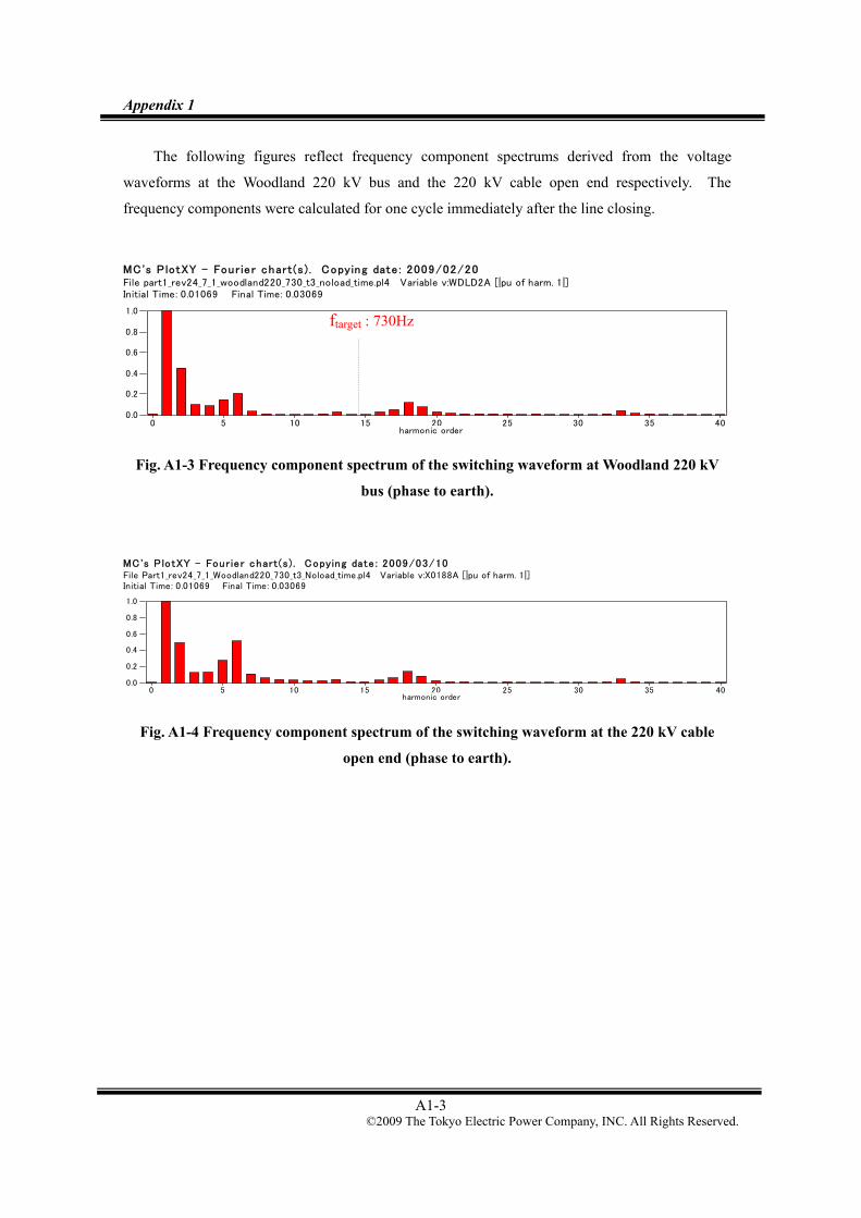
Appendix 1
A1-3 ©2009 The Tokyo Electric Power Company, INC. All Rights Reserved.
The following figures reflect frequency component spectrums derived from the voltage
waveforms at the Woodland 220 kV bus and the 220 kV cable open end respectively. The
frequency components were calculated for one cycle immediately after the line closing.
MC's P lotXY - Four ie r chart(s) . Copying date : 2009/02/20File part1_rev24_7_1_woodland220_730_t3_noload_time.pl4 Variable v:WDLD2A [|pu of harm. 1|]Initial Time: 0.01069 Final Time: 0.03069
0 5 10 15 20 25 30 35 400.0
0.2
0.4
0.6
0.8
1.0
harmonic order
Fig. A1-3 Frequency component spectrum of the switching waveform at Woodland 220 kV
bus (phase to earth).
MC's P lotXY - Four ie r chart(s) . Copying date : 2009/03/10File Part1_rev24_7_1_Woodland220_730_t3_Noload_time.pl4 Variable v:X0188A [|pu of harm. 1|]Initial Time: 0.01069 Final Time: 0.03069
0 5 10 15 20 25 30 35 400.0
0.2
0.4
0.6
0.8
1.0
harmonic order
Fig. A1-4 Frequency component spectrum of the switching waveform at the 220 kV cable
open end (phase to earth).
ftarget : 730Hz

Appendix 1
A1-4 ©2009 The Tokyo Electric Power Company, INC. All Rights Reserved.
Frequency scans were conducted from 10 Hz to 2000 Hz by 10 Hz step.
(file Part1_rev24_7_1_Woodland220_730_t3_Noload.pl4; x-var t) v:WDLD4A v:WDLD2A v:X0187A 0 400 800 1200 1600 2000
0
1000
2000
3000
4000
5000
(file Part1_rev24_7_1_Woodland220_730_t3_Noload.pl4; x-var t) v:WDLD4A v:WDLD2A v:X0187A 0 400 800 1200 1600 2000
0
100
200
300
400
500
Fig. A 1-5 Frequency scan at the Woodland 400 kV and 220 kV buses and 220 kV cable open
end (phase to earth).
Zoom
[Hz]
[Ω]
[Hz]
Impedance at 400 kV bus Impedance at 220 kV bus Impedance at 220 kV cable open
[Ω]
260Hz
900Hz 1650Hz

Appendix 1
A1-5 ©2009 The Tokyo Electric Power Company, INC. All Rights Reserved.
[Case (4)-1] Length of 220 kV cable: 7.625 km
(Phase to earth)
(file Part1_rev24_7_1_Woodland220_730_t8_Noload_time.pl4; x-var t) v:WDLD4A v:WDLD2A v:X0291A 0 10 20 30 40 50 60[ms]
-500
-375
-250
-125
0
125
250
375
500[kV]
Fig. A1-6 Switching waveforms at the Woodland 400 kV and 220 kV buses and 220 kV cable
open end (phase to earth).
(Phase to Phase)
(file Part1_rev24_7_1_Woodland220_730_t8_Noload_time.pl4; x-var t) v:WDLD2A-v:WDLD2B v:WDLD2B-v:WDLD2C v:WDLD2C-v:WDLD2A v:X0291A-v:X0291B v:X0291B-v:X0291C v:X0291C-v:X0291A
0 10 20 30 40 50 60[ms]-600
-400
-200
0
200
400
600
[kV]
(file Part1_rev24_7_1_Woodland220_730_t8_Noload_time.pl4; x-var t) v:WDLD2A-v:WDLD2B v:WDLD2B-v:WDLD2C v:WDLD2C-v:WDLD2A v:X0291A-v:X0291B v:X0291B-v:X0291C v:X0291C-v:X0291A
18.0 18.5 19.0 19.5 20.0 20.5 21.0 21.5 22.0[ms]450
470
490
510
530
550
[kV]
Fig. A1-7 Switching waveforms at the Woodland 220 kV bus and 220 kV cable open end
(phase to phase).
Voltage at 400 kV bus 490kV
Voltage at 220 kV bus 319kV
Voltage at 220 kV cable open end: 326kV
Voltage at 220 kV cable open end: 536kV
Voltage at 200 kV bus 513kV
Voltage at 220 kV cable open end: 536kV
Voltage at 200 kV bus 513kV
Zoom

Appendix 1
A1-6 ©2009 The Tokyo Electric Power Company, INC. All Rights Reserved.
The following figures show frequency component spectrums derived from the voltage
waveforms at the Woodland 220 kV bus and the 220 kV cable open end respectively. The
frequency components were calculated for one cycle immediately after the line closing.
MC's P lotXY - Four ie r chart(s) . Copying date : 2009/02/23File Part1_rev24_7_1_Woodland220_730_t8_Noload_time.pl4 Variable v:WDLD2A [peak]Initial Time: 0.0107 Final Time: 0.0307
0 5 10 15 20 25 30 35 400
50
100
150
200
[kV]
harmonic order
Fig. A1-8 Frequency component spectrum of the switching waveform at Woodland 220 kV
bus (phase to earth).
MC's P lotXY - Four ie r chart(s) . Copying date : 2009/02/26File Part1_rev24_7_1_Woodland220_730_t8_Noload_time.pl4 Variable v:X0291A [|pu of harm. 1|]Initial Time: 0.0107 Final Time: 0.0307
0 5 10 15 20 25 30 35 400.0
0.2
0.4
0.6
0.8
1.0
harmonic order
Fig. A1-9 Frequency component spectrum of the switching waveform at the 220 kV cable
open end (phase to earth).
950Hz
950Hz
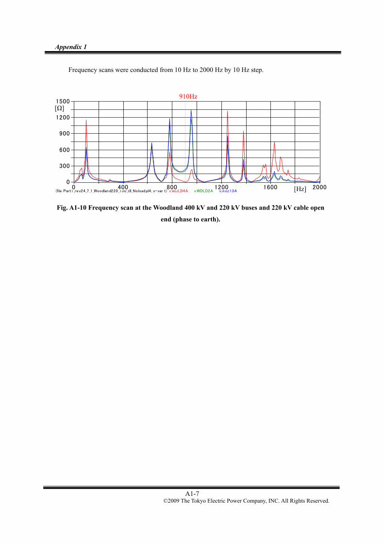
Appendix 1
A1-7 ©2009 The Tokyo Electric Power Company, INC. All Rights Reserved.
Frequency scans were conducted from 10 Hz to 2000 Hz by 10 Hz step.
(file Part1_rev24_7_1_Woodland220_730_t8_Noload.pl4; x-var t) v:WDLD4A v:WDLD2A v:X0213A 0 400 800 1200 1600 2000
0
300
600
900
1200
1500
Fig. A1-10 Frequency scan at the Woodland 400 kV and 220 kV buses and 220 kV cable open
end (phase to earth).
[Ω]
[Hz]
910Hz

Appendix 1
A1-8 ©2009 The Tokyo Electric Power Company, INC. All Rights Reserved.
[Case (4)-2] Length of 220 kV cable: 12 km
(Phase to earth)
(file Part1_rev24_7_1_Woodland220_730_t10_Noload_time.pl4; x-var t) v:WDLD4A v:WDLD2A v:X0056A 0 10 20 30 40 50 60[ms]
-500
-375
-250
-125
0
125
250
375
500[kV]
Fig. A1-11 Switching waveforms at the Woodland 400 kV and 220 kV buses and 220 kV cable
open end (phase to earth).
(Phase to phase)
(file Part1_rev24_7_1_Woodland220_730_t10_Noload_time.pl4; x-var t) v:WDLD2A-v:WDLD2B v:WDLD2B-v:WDLD2C v:WDLD2C-v:WDLD2A v:X0056A-v:X0056B v:X0056B-v:X0056C v:X0056C-v:X0056A
0 10 20 30 40 50 60[ms]-600
-380
-160
60
280
500
[kV]
Fig. A1-12 Switching waveforms at the and 220 kV bus and 220 kV cable open end (phase to
phase).
Voltage at 400 kV bus 476kV
Voltage at 220 kV bus 304kV
Voltage at 220 kV cable open end: 312kV
Voltage at 220 kV cable open end: 508kV
Voltage at 220 kV bus 489kV

Appendix 1
A1-9 ©2009 The Tokyo Electric Power Company, INC. All Rights Reserved.
MC's P lotXY - Four ie r chart(s) . Copying date : 2009/02/23File Part1_rev24_7_1_Woodland220_730_t10_Noload_time.pl4 Variable v:WDLD2A [|pu of harm. 1|]Initial Time: 0.0107 Final Time: 0.0307
0 5 10 15 20 25 30 35 400.0
0.2
0.4
0.6
0.8
1.0
harmonic order
Fig. A1-13 Frequency component spectrum of the switching waveform at Woodland 220 kV
bus (phase to earth).
MC's P lotXY - Four ie r chart(s) . Copying date : 2009/02/26File Part1_rev24_7_1_Woodland220_730_t10_Noload_time.pl4 Variable v:X0056A [|pu of harm. 1|]Initial Time: 0.0107 Final Time: 0.0307
0 5 10 15 20 25 30 35 400.0
0.2
0.4
0.6
0.8
1.0
harmonic order
Fig. A1-14 Frequency component spectrum of the switching waveform at the 220 kV cable
open end (phase to earth).
(file Part1_rev24_7_1_Woodland220_730_t10_Noload.pl4; x-var t) v:WDLD4A v:WDLD2A v:X0011A 0 400 800 1200 1600 2000
0
200
400
600
800
1000
1200
1400
1600
Fig. A1-15 Frequency scan at the Woodland 400 kV and 220 kV buses and 220 kV cable open
end (phase to earth).
[Ω]
[Hz]
710Hz
600Hz
600Hz
Impedance at 400 kV bus Impedance at 220 kV bus Impedance at 220 kV cable open

Appendix 1
A1-10 ©2009 The Tokyo Electric Power Company, INC. All Rights Reserved.
[Case (4)-3] Length of 220 kV cable: 15.25 km
(Phase to earth)
(file Part1_rev24_7_1_Woodland220_730_t7_Noload_time.pl4; x-var t) v:WDLD4A v:WDLD2A v:X0165A 0 10 20 30 40 50 60[ms]
-400
-250
-100
50
200
350
500[kV]
Fig. A1-16 Switching waveforms at the Woodland 400 kV and 220 kV buses and 220 kV cable
open end (phase to earth)..
(Phase to phase)
(file Part1_rev24_7_1_Woodland220_730_t7_Noload_time.pl4; x-var t) v:WDLD2A-v:WDLD2B v:WDLD2B-v:WDLD2C v:WDLD2C-v:WDLD2A v:X0165A-v:X0165B v:X0165B-v:X0165C v:X0165C-v:X0165A
0 10 20 30 40 50 60[ms]-600
-400
-200
0
200
400
600
[kV]
Fig. A1-17 Switching waveforms at the Woodland 220 kV bus and 220 kV cable open end
(phase to phase).
Voltage at 400 kV bus 458kV
Voltage at 220 kV bus 321kV
Voltage at 220 kV cable open end: 328kV
Voltage at 220 kV cable open end: 532kV
Voltage at 220 kV bus 522kV

Appendix 1
A1-11 ©2009 The Tokyo Electric Power Company, INC. All Rights Reserved.
MC's P lotXY - Four ie r chart(s) . Copying date : 2009/02/23File Part1_rev24_7_1_Woodland220_730_t7_Noload_time.pl4 Variable v:WDLD2A [|pu of harm. 1|]Initial Time: 0.0107 Final Time: 0.0307
0 5 10 15 20 25 30 35 400.0
0.2
0.4
0.6
0.8
1.0
harmonic order
Fig. A1-18 Frequency component spectrum of the switching waveform at Woodland 220 kV
bus (phase to earth).
MC's P lotXY - Four ie r chart(s) . Copying date : 2009/02/25File Part1_rev24_7_1_Woodland220_730_t7_Noload_time.pl4 Variable v:X0165A [|pu of harm. 1|]Initial Time: 0.0107 Final Time: 0.0307
0 5 10 15 20 25 30 35 400.0
0.2
0.4
0.6
0.8
1.0
harmonic order
Fig. A1-19 Frequency component spectrum of the switching waveform at the 220 kV cable
open end (phase to earth).
(file Part1_rev24_7_1_Woodland220_730_t7_Noload.pl4; x-var t) v:WDLD4A v:WDLD2A v:X0213A 0 400 800 1200 1600 2000
0
300
600
900
1200
1500
Fig. A1-20 Frequency scan at the Woodland 400 kV and 220 kV buses and 220 kV cable open
end (phase to earth).
[Ω]
[Hz]
560Hz
620Hz
550Hz
550Hz
Impedance at 400 kV bus Impedance at 220 kV bus Impedance at 220 kV cable open

Appendix 1
A1-12 ©2009 The Tokyo Electric Power Company, INC. All Rights Reserved.
[Case (4)-4] Length of 220 kV cable: 30.5km
(Phase to earth)
(file Part1_rev24_7_1_Woodland220_730_t11_Noload_time.pl4; x-var t) v:WDLD4A v:WDLD2A v:X0056A 0 10 20 30 40 50 60[ms]
-400
-250
-100
50
200
350
500[kV]
Fig. A1-21 Switching waveforms at the Woodland 400 kV and 220 kV buses and 220 kV cable
open end (phase to earth).
(Phase to phase)
(file Part1_rev24_7_1_Woodland220_730_t11_Noload_time.pl4; x-var t) v:WDLD2A-v:WDLD2B v:WDLD2B-v:WDLD2C v:WDLD2C-v:WDLD2A v:X0056A-v:X0056B v:X0056B-v:X0056C v:X0056C-v:X0056A
0 10 20 30 40 50 60[ms]-800
-600
-400
-200
0
200
400
600
800[kV]
Fig. A1-22 Switching waveforms at the Woodland 220 kV bus and 220 kV cable open end
(phase to phase).
Voltage at 400 kV bus 467kV
Voltage at 220 kV bus 354kV
Voltage at 220 kV cable open end: 375kV
Voltage at 220 kV bus 549kV

Appendix 1
A1-13 ©2009 The Tokyo Electric Power Company, INC. All Rights Reserved.
MC's P lotXY - Four ie r chart(s) . Copying date : 2009/02/23File Part1_rev24_7_1_Woodland220_730_t11_Noload_time.pl4 Variable v:WDLD2A [|pu of harm. 1|]Initial Time: 0.0107 Final Time: 0.0307
0 5 10 15 20 25 30 35 400.0
0.2
0.4
0.6
0.8
1.0
harmonic order
Fig. A1-23 Frequency component spectrum of the switching waveform at Woodland 220 kV bus (phase to earth).
MC's P lotXY - Four ie r chart(s) . Copying date : 2009/02/25File Part1_rev24_7_1_Woodland220_730_t11_Noload_time.pl4 Variable v:X0056A [|pu of harm. 1|]Initial Time: 0.0107 Final Time: 0.0307
0 5 10 15 20 25 30 35 400.0
0.2
0.4
0.6
0.8
1.0
harmonic order
Fig. A1-24 Frequency component spectrum of the switching waveform at the 220 kV cable open end (phase to earth).
(file Part1_rev24_7_1_Woodland220_730_t11_Noload.pl4; x-var t) v:WDLD4A v:WDLD2A v:X0150A 0 400 800 1200 1600 2000
0
600
1200
1800
(file Part1_rev24_7_1_Woodland220_730_t11_Noload.pl4; x-var t) v:WDLD4A v:WDLD2A v:X0150A 0 400 800 1200 1600 2000
0
100
200
300
400
500
Fig. A1-25 Frequency scan at the Woodland 400 kV and 220 kV buses and 220 kV cable open end (phase to earth).
Zoom
[Hz]
[Ω]
[Ω]
[Hz]
Impedance at 400 kV bus Impedance at 220 kV bus Impedance at 220 kV cable open
400Hz
400Hz
420Hz

Appendix 1
A1-14 ©2009 The Tokyo Electric Power Company, INC. All Rights Reserved.
[Case (4)-5] Cable length: (Length of the base case) * 1.5 = 91.5 km
(Phase to earth)
(file Part1_rev24_7_1_Woodland220_730_t6_Noload_time.pl4; x-var t) v:WDLD4A v:WDLD2A v:X0149A 0 10 20 30 40 50 60[ms]
-400
-300
-200
-100
0
100
200
300
400[kV]
Fig. A1-26 Switching waveforms at the Woodland 400 kV and 220 kV buses and 220 kV cable
open end (phase to earth).
(Phase to phase)
(file Part1_rev24_7_1_Woodland220_730_t6_Noload_time.pl4; x-var t) v:WDLD2A-v:WDLD2B v:WDLD2A-v:WDLD2C v:WDLD2C-v:WDLD2A v:X0149A-v:X0149B v:X0149B-v:X0149C v:X0149C v:X0149A
0 10 20 30 40 50 60[ms]-600
-400
-200
0
200
400
600
[kV]
Fig. A1-27 Switching waveforms at the Woodland 220 kV bus and 220 kV cable open end
(phase to phase).
Voltage at 220 kV bus 257kV
Voltage at 400 kV bus 384kV
Voltage at 220 kV cable open end: 350kV
Voltage at 220 kV cable open end: 501kV
Voltage at 220 kV bus 429kV
V4

Appendix 1
A1-15 ©2009 The Tokyo Electric Power Company, INC. All Rights Reserved.
MC's P lotXY - Four ie r chart(s) . Copying date : 2009/02/20File Part1_rev24_7_1_Woodland220_730_t6_Noload_time.pl4 Variable v:WDLD2A [|pu of harm. 1|]Initial Time: 0.01069 Final Time: 0.03069
0 5 10 15 20 25 30 35 400.0
0.2
0.4
0.6
0.8
1.0
harmonic order
Fig. A1-28 Frequency component spectrum of the switching waveform at Woodland 220 kV
bus (phase to earth).
MC's P lotXY - Four ie r chart(s) . Copying date : 2009/02/25File Part1_rev24_7_1_Woodland220_730_t6_Noload_time.pl4 Variable v:X0149A [|pu of harm. 1|]Initial Time: 0.01069 Final Time: 0.03069
0 5 10 15 20 25 30 35 400.0
0.2
0.4
0.6
0.8
1.0
harmonic order
Fig. A1-29 Frequency component spectrum of the switching waveform at the 220 kV cable
open end (phase to earth).
(file Part1_rev24_7_1_Woodland220_730_t6_Noload.pl4; x-var t) v:WDLD2A v:X0226A v:WDLD4A 0 400 800 1200 1600 2000
0
200
400
600
800
1000
1200
Fig. A1-30 Frequency scan at the Woodland 400 kV and 220 kV buses and 220 kV cable open
end (phase to earth).
600Hz
[Ω]
[Hz]
Impedance at 400 kV bus Impedance at 220 kV bus Impedance at 220 kV cable open
600Hz
630Hz200Hz

Appendix 1
A1-16 ©2009 The Tokyo Electric Power Company, INC. All Rights Reserved.
[Case (4)-6] Cable length: (Length of the base case) * 2 = 122 km
(Phase to earth)
(file Part1_rev24_7_1_Woodland220_730_t12_Noload_time.pl4; x-var t) v:WDLD4A v:WDLD2A v:X0149A 0 10 20 30 40 50 60[ms]
-500
-375
-250
-125
0
125
250
375
500[kV]
Fig. A1-31 The switching waveforms at the Woodland 400 kV and 220 kV buses and 220 kV
cable open end (phase to earth).
(Phase to phase)
(file Part1_rev24_7_1_Woodland220_730_t12_Noload_time.pl4; x-var t) v:WDLD2A-v:WDLD2B v:WDLD2B-v:WDLD2C v:WDLD2C-v:WDLD2A v:X0149A-v:X0149B v:X0149B-v:X0149C v:X0149C-v:X0149A
0 10 20 30 40 50 60[ms]-600
-400
-200
0
200
400
600
[kV]
Fig. A1-32 The switching waveforms at the Woodland 220 kV bus and 220 kV cable open end
(phase to phase).
Voltage at 220 kV bus 235kV
Voltage at 400 kV bus 431kV
Voltage at 220 kV cable open end: 311kV
Voltage at 220 kV bus 385kV
Voltage at 220 kV cable open end: 547kV

Appendix 1
A1-17 ©2009 The Tokyo Electric Power Company, INC. All Rights Reserved.
MC's P lotXY - Four ie r chart(s) . Copying date : 2009/02/25File Part1_rev24_7_1_Woodland220_730_t12_Noload_time.pl4 Variable v:WDLD2A [peak]Initial Time: 0.01069 Final Time: 0.03069
0 5 10 15 20 25 30 35 40-20
30
80
130
180
[kV]
harmonic order
Fig. A1-33 Frequency component spectrum of the switching waveform at Woodland 220 kV
bus (phase to earth).
MC's P lotXY - Four ie r chart(s) . Copying date : 2009/02/25File Part1_rev24_7_1_Woodland220_730_t12_Noload_time.pl4 Variable v:X0149A [|pu of harm. 1|]Initial Time: 0.01069 Final Time: 0.03069
0 5 10 15 20 25 30 35 400.0
0.2
0.4
0.6
0.8
1.0
harmonic order
Fig. A1-34 Frequency component spectrum of the switching waveform at the 220 kV cable
open end (phase to earth).
(file Part1_rev24_7_1_Woodland220_730_t12_Noload.pl4; x-var t) v:WDLD4A v:WDLD2A v:X0213A 0 400 800 1200 1600 2000
0
150
300
450
600
750
900
Fig. A1-35 Frequency scan at the Woodland 400 kV and 220 kV buses and 220 kV cable open
end (phase to earth).
[Hz]
Impedance at 400 kV bus Impedance at 220 kV bus Impedance at 220 kV cable open
490Hz
500Hz
500Hz
160Hz

Appendix 1
A1-18 ©2009 The Tokyo Electric Power Company, INC. All Rights Reserved.
[Case (4)-7] Cable length: (Length of the base case) * 3 = 183 km
(Phase to earth)
(file Part1_rev24_7_1_Woodland220_730_t13_Noload_time.pl4; x-var t) v:WDLD4A v:WDLD2A v:X0293A 0 10 20 30 40 50 60[ms]
-400
-300
-200
-100
0
100
200
300
400[kV]
Fig. A1-36 Switching waveforms at the Woodland 400 kV and 220 kV buses and 220 kV cable
open end (phase to earth).
(Phase to Phase)
(file Part1_rev24_7_1_Woodland220_730_t13_Noload_time.pl4; x-var t) v:WDLD2A-v:WDLD2B v:WDLD2B-v:WDLD2C v:WDLD2C-v:WDLD2A v:X0293A-v:X0293B v:X0293B-v:X0293C v:X0293C-v:X0293A
0 10 20 30 40 50 60[ms]-600
-400
-200
0
200
400
600
[kV]
Fig. A1-37 Switching waveforms at the Woodland 220 kV bus and 220 kV cable open end
(phase to earth).
Voltage at 220 kV bus 212kV
Voltage at 400 kV bus388kV
Voltage at 220 kV cable open end: -331kV
Voltage at 220 kV cable open end: 545kV
Voltage at 220 kV bus 415kV

Appendix 1
A1-19 ©2009 The Tokyo Electric Power Company, INC. All Rights Reserved.
MC's P lotXY - Four ie r chart(s) . Copying date : 2009/02/25File Part1_rev24_7_1_Woodland220_730_t13_Noload_time.pl4 Variable v:WDLD2A [|pu of harm. 1|]Initial Time: 0.01069 Final Time: 0.03069
0 5 10 15 20 25 300.0
0.2
0.4
0.6
0.8
1.0
harmonic order
Fig. A1-38 Frequency component spectrum of the switching waveform at Woodland 220 kV
bus (phase to earth).
MC's P lotXY - Four ie r chart(s) . Copying date : 2009/02/25File Part1_rev24_7_1_Woodland220_730_t13_Noload_time.pl4 Variable v:X0293A [|pu of harm. 1|]Initial Time: 0.01069 Final Time: 0.03069
0 5 10 15 20 25 30 35 400.0
0.2
0.4
0.6
0.8
1.0
harmonic order
Fig. A1-39 Frequency component spectrum of the switching waveform at the 220 kV cable
open end (phase to earth).
(file Part1_rev24_7_1_Woodland220_730_t13_Noload.pl4; x-var t) v:WDLD4A v:WDLD2A v:X0340A 0 400 800 1200 1600 2000
0
300
600
900
1200
1500
Fig. A1-40 Frequency scan at the Woodland 400 kV and 220 kV buses and 220 kV cable open
end (phase to earth).
Impedance at 400 kV bus Impedance at 220 kV bus Impedance at 220 kV cable open
[Ω]
[Hz]
120Hz 340Hz

Appendix 1
A1-20 ©2009 The Tokyo Electric Power Company, INC. All Rights Reserved.
[Case (4)-8] Cable length: (Length of the base case) * 4 = 244 km
(Phase to earth)
(file Part1_rev24_7_1_Woodland220_730_t14_Noload_time.pl4; x-var t) v:WDLD2A v:X0294A v:WDLD4A 0 10 20 30 40 50 60[ms]
-500
-375
-250
-125
0
125
250
375
500[kV]
Fig. A1-41 Switching waveforms at the Woodland 400 kV and 220 kV buses and the 220 kV
cable open end (phase to earth).
(Phase to phase)
(file Part1_rev24_7_1_Woodland220_730_t14_Noload_time.pl4; x-var t) v:WDLD2A-v:WDLD2B v:WDLD2B-v:WDLD2C v:WDLD2C-v:WDLD2A v:X0294A-v:X0294B v:X0294B-v:X0294C v:X0294C-v:X0294A
0 10 20 30 40 50 60[ms]-600
-400
-200
0
200
400
600
[kV]
Fig. A1-42 Switching waveforms at the Woodland 220 kV bus and the 220 kV cable open end
(phase to phase).
Voltage at 220 kV bus: 234kV
Voltage at 400 kV bus -416kV
Voltage at 220 kV cable open end: 309kV
Voltage at 220 kV bus416kV
Voltage at 220 kV cable open end: 495kV

Appendix 1
A1-21 ©2009 The Tokyo Electric Power Company, INC. All Rights Reserved.
MC's P lotXY - Four ie r chart(s) . Copying date : 2009/02/25File Part1_rev24_7_1_Woodland220_730_t14_Noload_time.pl4 Variable v:WDLD2A [|pu of harm. 1|]Initial Time: 0.01069 Final Time: 0.03069
0 5 10 15 20 25 30 35 400.0
0.2
0.4
0.6
0.8
1.0
harmonic order
Fig. A1-43 Frequency component spectrum of the switching waveform at Woodland 220 kV
bus (phase to earth).
MC's P lotXY - Four ie r chart(s) . Copying date : 2009/02/25File Part1_rev24_7_1_Woodland220_730_t14_Noload_time.pl4 Variable v:X0294A [|pu of harm. 1|]Initial Time: 0.01069 Final Time: 0.03069
0 5 10 15 20 25 30 35 400.0
0.2
0.4
0.6
0.8
1.0
harmonic order
Fig. A1-44 Frequency component spectrum of the switching waveform at the 220 kV cable
open end (phase to earth).
(file Part1_rev24_7_1_Woodland220_730_t14_Noload.pl4; x-var t) v:WDLD4A v:WDLD2A v:X0340A 0 400 800 1200 1600 2000
0
200
400
600
800
1000
1200
1400
Fig. A1-45 Frequency scan at the Woodland 400 kV and 220 kV buses and the 220 kV cable
open end (phase to earth).
[Ω]
[Hz]
Impedance at 400 kV bus Impedance at 220 kV bus Impedance at 220 kV cable open
120Hz

Appendix 2
A2-1 ©2009 The Tokyo Electric Power Company, INC. All Rights Reserved.
Appendix 2 Results of the Parametric Study on the 400 kV
Woodland – Kingscourt Cable Length
Frequency scans and time domain simulations of the 400 kV Woodland – Kingscourt line
energisation were performed with different lengths of the 400 kV Woodland – Kingscourt cable.
The results of the parametric study have been summarized in Section 3.1.1 of the Part 1 report.
All the figures obtained in the parametric study are shown in Appendix 2.
List of the 220 kV Woodland – Louth cable length assumed in the study is shown in Table
A2-1.
Table A2-1 List of the 400 kV Woodland – Kingscourt Cable Length
Woodland Kingscourt(5)- 1 141.7 km 300 Hz 1,317 MVA 750 MVA 600 MVA 102.5%(5)- 2 106.3 km 400 Hz 988 MVA 600 MVA 360 MVA 97.2%(5)- 3 85.0 km 500 Hz 790 MVA 450 MVA 360 MVA 102.5%(5)- 4 70.8 km 600 Hz 659 MVA 300 MVA 360 MVA 100.2%(5)- 5 60.7 km 700 Hz 564 MVA 300 MVA 300 MVA 106.3%(5)- 6 47.2 km 900 Hz 439 MVA 300 MVA 120 MVA 95.7%(5)- 7 38.6 km 1100 Hz 359 MVA 240 MVA 120 MVA 100.2%(5)- 8 26.6 km 1600 Hz 247 MVA 120 MVA 120 MVA 97.2%(5)- 9 22.4 km 1900 Hz 208 MVA 120 MVA 120 MVA 115.4%
9.3 MVA/cct/km
400kVcable
Targetfrequency
Chargingcapacity
Charging capacity:
Compensationrate
Reactor for 400kV cable

Appendix 2
A2-2 ©2009 The Tokyo Electric Power Company, INC. All Rights Reserved.
[Case (5)-1] Total 400 kV cable length: 141.7 km, Target frequency: 300 Hz
(Phase to earth)
(file Part1_rev24_7_1_Woodland220_xxx300_13_01_time.pl4; x-var t) v:WDLD4A v:WDLD2A v:X0204A 0 10 20 30 40 50 60[ms]
-400
-300
-200
-100
0
100
200
300
400[kV]
Fig. A2-1 Switching waveforms at the Woodland 400 kV and 220 kV buses and the 220 kV
cable open end (Phase to earth).
(Phase to phase)
(file Part1_rev24_7_1_Woodland220_xxx300_13_01_time.pl4; x-var t) v:WDLD2A-v:WDLD2B v:WDLD2B-v:WDLD2C v:WDLD2C-v:WDLD2A v:X0204A-v:X0204B v:X0204B-v:X0204C v:X0204C-v:X0204A
0 10 20 30 40 50 60[ms]-400
-300
-200
-100
0
100
200
300
400[kV]
Fig. A2-2 Switching waveforms at the Woodland 220 kV bus and the 220 kV cable open end
(phase to phase).
Voltage at 220 kV bus
Voltage at 220 kV cable open end: 243kV
Voltage at 400 kV cable open end: 338kV
Voltage at 220 kV cable open end: 381kV
Voltage at 220 kV bus 362kV

Appendix 2
A2-3 ©2009 The Tokyo Electric Power Company, INC. All Rights Reserved.
MC's P lotXY - Four ie r chart(s) . Copying date : 2009/02/27File Part1_rev24_7_1_Woodland220_xxx300_13_01_time.pl4 Variable v:WDLD2A [|pu of harm. 1|]Initial Time: 0.011 Final Time: 0.031
0 5 10 15 20 25 30 35 400.0
0.2
0.4
0.6
0.8
1.0
harmonic order
Fig. A2-3 Frequency component spectrum of the switching waveform at Woodland 220 kV
bus (phase to earth).
MC's P lotXY - Four ie r chart(s) . Copying date : 2009/02/27File Part1_rev24_7_1_Woodland220_xxx300_13_01_time.pl4 Variable v:X0204A [|pu of harm. 1|]Initial Time: 0.011 Final Time: 0.031
0 5 10 15 20 25 30 35 400.0
0.2
0.4
0.6
0.8
1.0
harmonic order
Fig. A2-4 Frequency component spectrum of the switching waveform at the 220 kV cable
open end (phase to earth).
(file Part1_rev24_7_1_Woodland220_xxx300_13_01.pl4; x-var t) v:WDLD4A v:WDLD2A v:X0187A 0 400 800 1200 1600 2000
0
100
200
300
400
500
Fig. A2-5 Frequency scan at the Woodland 400 kV and 220 kV buses and 220 kV cable open
end (phase to earth).
260Hz 900Hz[Ω]
[Hz]

Appendix 2
A2-4 ©2009 The Tokyo Electric Power Company, INC. All Rights Reserved.
[Case (5)-2] Total 400 kV cable length: 106.3 km, Target frequency: 400 Hz
(Phase to earth)
(file Part1_rev24_7_1_Woodland220_xxx400_13_01_time.pl4; x-var t) v:WDLD4A v:WDLD2A v:X0198A 0 10 20 30 40 50 60[ms]
-400
-300
-200
-100
0
100
200
300
400[kV]
Fig. A2-6 Switching waveforms at the Woodland 400 kV and 220 kV buses and the 220 kV
cable open end (phase to earth).
(Phase to phase)
(file Part1_rev24_7_1_Woodland220_xxx400_13_01_time.pl4; x-var t) v:WDLD2A-v:WDLD2B v:WDLD2B-v:WDLD2C v:WDLD2C-v:WDLD2A v:X0198A-v:X0198B v:X0198B-v:X0198C v:X0198C-v:X0198A
0 10 20 30 40 50 60[ms]-600
-400
-200
0
200
400
600
[kV]
Fig. A2-7 Switching waveforms at the Woodland 220 kV buses and the 220 kV cable open end
(phase to phase).
Voltage at 220 kV bus
Voltage at 220 kV cable open end: 279kVVoltage at 400 kV cable
open end: 378kV
Voltage at 220 kV bus 421kV Voltage at 220 kV cable
open end: 491kV
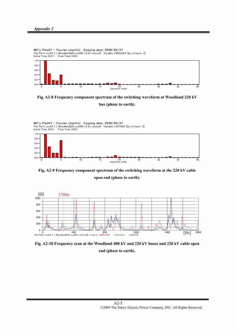
Appendix 2
A2-5 ©2009 The Tokyo Electric Power Company, INC. All Rights Reserved.
MC's P lotXY - Four ie r chart(s) . Copying date : 2009/02/27File Part1_rev24_7_1_Woodland220_xxx400_13_01_time.pl4 Variable v:WDLD2A [|pu of harm. 1|]Initial Time: 0.011 Final Time: 0.031
0 5 10 15 20 25 30 35 400.0
0.2
0.4
0.6
0.8
1.0
harmonic order
Fig. A2-8 Frequency component spectrum of the switching waveform at Woodland 220 kV
bus (phase to earth).
MC's P lotXY - Four ie r chart(s) . Copying date : 2009/02/27File Part1_rev24_7_1_Woodland220_xxx400_13_01_time.pl4 Variable v:X0198A [|pu of harm. 1|]Initial Time: 0.011 Final Time: 0.031
0 5 10 15 20 25 30 35 400.0
0.2
0.4
0.6
0.8
1.0
harmonic order
Fig. A2-9 Frequency component spectrum of the switching waveform at the 220 kV cable
open end (phase to earth).
(file Part1_rev24_7_1_Woodland220_xxx400_13_01.pl4; x-var t) v:WDLD4A v:WDLD2A v:X0187A 0 400 800 1200 1600 2000
0
200
400
600
800
1000
Fig. A2-10 Frequency scan at the Woodland 400 kV and 220 kV buses and 220 kV cable open
end (phase to earth).
270Hz[Ω]
[Hz]

Appendix 2
A2-6 ©2009 The Tokyo Electric Power Company, INC. All Rights Reserved.
[Case (5)-3] Total 400 kV cable length: 85 km, Target frequency: 500 Hz
(Phase to earth)
(file Part1_rev24_7_1_Woodland220_xxx500_13_01_time.pl4; x-var t) v:WDLD4A v:WDLD2A v:X0196A 0 10 20 30 40 50 60[ms]
-400
-300
-200
-100
0
100
200
300
400[kV]
Fig. A2-11 Switching waveforms at the Woodland 400 kV and 220 kV buses and the 220 kV
cable open end (phase to earth).
(Phase to phase)
(file Part1_rev24_7_1_Woodland220_xxx500_13_01_time.pl4; x-var t) v:WDLD2A-v:WDLD2B v:WDLD2B-v:WDLD2C v:WDLD2C-v:WDLD2A v:X0196A-v:X0196B v:X0196B-v:X0196C v:X0196C-v:X0196A
0 10 20 30 40 50 60[ms]-600
-400
-200
0
200
400
600
[kV]
Fig. A2-12 Switching waveforms at the Woodland 220 kV bus and the 220 kV cable open end
(phase to phase).
Voltage at 220 kV bus: 260kV
Voltage at 220 kV cable open end: 326kV
Voltage at 400 kV cable open end: 383kV
Voltage at 220 kV cable open end: 529kV
Voltage at 220 kV bus 443kV

Appendix 2
A2-7 ©2009 The Tokyo Electric Power Company, INC. All Rights Reserved.
MC's P lotXY - Four ie r chart(s) . Copying date : 2009/02/27File Part1_rev24_7_1_Woodland220_xxx500_13_01_time.pl4 Variable v:WDLD2A [|pu of harm. 1|]Initial Time: 0.011 Final Time: 0.031
0 5 10 15 20 25 30 35 400.0
0.2
0.4
0.6
0.8
1.0
harmonic order
Fig. A2-13 Frequency component spectrum of the switching waveform at Woodland 220 kV
bus (phase to earth).
MC's P lotXY - Four ie r chart(s) . Copying date : 2009/02/27File Part1_rev24_7_1_Woodland220_xxx500_13_01_time.pl4 Variable v:X0196A [|pu of harm. 1|]Initial Time: 0.011 Final Time: 0.031
0 5 10 15 20 25 30 35 400.0
0.2
0.4
0.6
0.8
1.0
harmonic order
Fig. A2-14 Frequency component spectrum of the switching waveform at the 220 kV cable
open end (phase to earth).
(file Part1_rev24_7_1_Woodland220_xxx500_13_01.pl4; x-var t) v:WDLD4A v:WDLD2A v:X0187A 0 400 800 1200 1600 2000
0
400
800
1200
1600
2000
Fig. A2-15 Frequency scan at the Woodland 400 kV and 220 kV buses and 220 kV cable open
end (phase to earth).
900Hz260Hz
[Hz]

Appendix 2
A2-8 ©2009 The Tokyo Electric Power Company, INC. All Rights Reserved.
[Case (5)-4] Total 400 kV cable length: 70.8 km, Target frequency: 600 Hz
(Phase to earth)
(file Part1_rev24_7_1_Woodland220_xxx600_13_01_time.pl4; x-var t) v:WDLD4A v:WDLD2A v:X0194A 0 10 20 30 40 50 60[ms]
-400
-250
-100
50
200
350
500
[kV]
Fig. A2-16 Switching waveforms at the Woodland 400 kV and 220 kV buses and the 220 kV
cable open end (phase to earth).
(Phase to Phase)
(file Part1_rev24_7_1_Woodland220_xxx600_13_01_time.pl4; x-var t) v:WDLD2A-v:WDLD2B v:WDLD2B-v:WDLD2C v:WDLD2C-v:WDLD2A v:X0194A-v:X0194B v:X0194B-v:X0194C v:X0194C-v:X0194A
0 10 20 30 40 50 60[ms]-600
-400
-200
0
200
400
600
[kV]
Fig. A2-17 Switching waveforms at the Woodland 220 kV bus and the 220 kV cable open end
(phase to phase).
Voltage at 220 kV bus: 278kV
Voltage at 220 kV cable open end: 285kV
Voltage at 400 kV cable open end: 430kV
Voltage at 220 kV bus: 502kV
Voltage at 220 kV bus 550kV
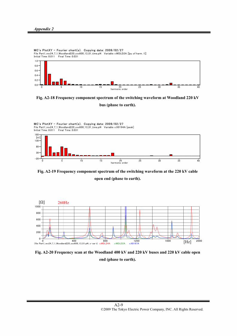
Appendix 2
A2-9 ©2009 The Tokyo Electric Power Company, INC. All Rights Reserved.
MC's P lotXY - Four ie r chart(s) . Copying date : 2009/02/27File Part1_rev24_7_1_Woodland220_xxx600_13_01_time.pl4 Variable v:WDLD2A [|pu of harm. 1|]Initial Time: 0.011 Final Time: 0.031
0 5 10 15 20 25 30 35 400.0
0.2
0.4
0.6
0.8
1.0
harmonic order
Fig. A2-18 Frequency component spectrum of the switching waveform at Woodland 220 kV
bus (phase to earth).
MC's P lotXY - Four ie r chart(s) . Copying date : 2009/02/27File Part1_rev24_7_1_Woodland220_xxx600_13_01_time.pl4 Variable v:X0194A [peak]Initial Time: 0.011 Final Time: 0.031
0 5 10 15 20 25 30 35 40-20
30
80
130
180[kV]
harmonic order
Fig. A2-19 Frequency component spectrum of the switching waveform at the 220 kV cable
open end (phase to earth).
(file Part1_rev24_7_1_Woodland220_xxx600_13_01.pl4; x-var t) v:WDLD4A v:WDLD2A v:X0187A 0 400 800 1200 1600 2000
0
200
400
600
800
1000
Fig. A2-20 Frequency scan at the Woodland 400 kV and 220 kV buses and 220 kV cable open
end (phase to earth).
260Hz [Ω]
[Hz]

Appendix 2
A2-10 ©2009 The Tokyo Electric Power Company, INC. All Rights Reserved.
[Case (5)-5] Total 400 kV cable length: 60.7 km, Target frequency: 700 Hz
(Phase to earth)
(file Part1_rev24_7_1_Woodland220_xxx700_13_01_time.pl4; x-var t) v:WDLD4A v:WDLD2A v:X0192A 0 10 20 30 40 50 60[ms]
-500
-375
-250
-125
0
125
250
375
500[kV]
Fig. A2-21 Switching waveforms at the Woodland 400 kV and 220 kV buses and the 220 kV
cable open end (phase to earth).
(Phase to phase)
(file Part1_rev24_7_1_Woodland220_xxx700_13_01_time.pl4; x-var t) v:WDLD2A-v:WDLD2B v:WDLD2B-v:WDLD2C v:WDLD2C-v:WDLD2A v:X0192A-v:X0192B v:X0192B-v:X0192C v:X0192C-v:X0192A
0 10 20 30 40 50 60[ms]-600
-400
-200
0
200
400
600
[kV]
Fig. A2-22 Switching waveforms at the Woodland 220 kV bus and the 220 kV cable open end
(phase to phase).
Voltage at 220 kV bus
Voltage at 220 kV cable open end: 322kV
Voltage at 400 kV cable open end: 444kV
Voltage at 220 kV bus: 478kV
Voltage at 220 kV cable open end: 598kV

Appendix 2
A2-11 ©2009 The Tokyo Electric Power Company, INC. All Rights Reserved.
MC's P lotXY - Four ie r chart(s) . Copying date : 2009/02/27File Part1_rev24_7_1_Woodland220_xxx700_13_01_time.pl4 Variable v:WDLD2A [|pu of harm. 1|]Initial Time: 0.0117 Final Time: 0.0317
0 5 10 15 20 25 30 35 400.0
0.2
0.4
0.6
0.8
1.0
harmonic order
Fig. A2-23 Frequency component spectrum of the switching waveform at Woodland 220 kV
bus (phase to earth).
MC's P lotXY - Four ie r chart(s) . Copying date : 2009/02/27File Part1_rev24_7_1_Woodland220_xxx700_13_01_time.pl4 Variable v:X0192A [|pu of harm. 1|]Initial Time: 0.0117 Final Time: 0.0317
0 5 10 15 20 25 30 35 400.0
0.2
0.4
0.6
0.8
1.0
harmonic order
Fig. A2-24 Frequency component spectrum of the switching waveform at the 220 kV cable
open end (phase to earth).
(file Part1_rev24_7_1_Woodland220_xxx700_13_01.pl4; x-var t) v:WDLD4A v:WDLD2A v:X0187A 0 400 800 1200 1600 2000
0
200
400
600
800
1000
Fig. A2-25 Frequency scan at the Woodland 400 kV and 220 kV buses and 220 kV cable open
end (phase to earth).
260Hz [Ω]
[Hz]
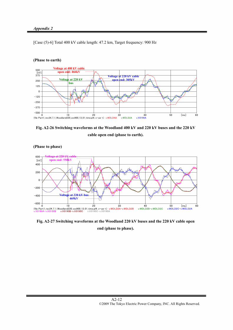
Appendix 2
A2-12 ©2009 The Tokyo Electric Power Company, INC. All Rights Reserved.
[Case (5)-6] Total 400 kV cable length: 47.2 km, Target frequency: 900 Hz
(Phase to earth)
(file Part1_rev24_7_1_Woodland220_xxx900_13_01_time.pl4; x-var t) v:WDLD4A v:WDLD2A v:X0190A 0 10 20 30 40 50 60[ms]
-500
-375
-250
-125
0
125
250
375
500[kV]
Fig. A2-26 Switching waveforms at the Woodland 400 kV and 220 kV buses and the 220 kV
cable open end (phase to earth).
(Phase to phase)
(file Part1_rev24_7_1_Woodland220_xxx900_13_01_time.pl4; x-var t) v:WDLD2A-v:WDLD2B v:WDLD2B-v:WDLD2C v:WDLD2C-v:WDLD2A v:X0190A-v:X0190B v:X0190B-v:X0190C v:X0190C-v:X0190A
0 10 20 30 40 50 60[ms]-600
-400
-200
0
200
400
600
[kV]
Fig. A2-27 Switching waveforms at the Woodland 220 kV buses and the 220 kV cable open
end (phase to phase).
Voltage at 220 kV bus
Voltage at 220 kV cable open end: 305kV
Voltage at 400 kV cable open end: 466kV
Voltage at 220 kV cable open end: 550kV
Voltage at 220 kV bus 469kV

Appendix 2
A2-13 ©2009 The Tokyo Electric Power Company, INC. All Rights Reserved.
MC's P lotXY - Four ie r chart(s) . Copying date : 2009/02/27File Part1_rev24_7_1_Woodland220_xxx900_13_01_time.pl4 Variable v:WDLD2A [|pu of harm. 1|]Initial Time: 0.01155 Final Time: 0.03155
0 5 10 15 20 25 30 35 400.0
0.2
0.4
0.6
0.8
1.0
harmonic order
Fig. A2-28 Frequency component spectrum of the switching waveform at Woodland 220 kV
bus (phase to earth).
MC's P lotXY - Four ie r chart(s) . Copying date : 2009/02/27File Part1_rev24_7_1_Woodland220_xxx900_13_01_time.pl4 Variable v:X0190A [|pu of harm. 1|]Initial Time: 0.01155 Final Time: 0.03155
0 5 10 15 20 25 30 35 400.0
0.2
0.4
0.6
0.8
1.0
harmonic order
Fig. A2-29 Frequency component spectrum of the switching waveform at the 220 kV cable
open end (phase to earth).
(file Part1_rev24_7_1_Woodland220_xxx900_13_01x.pl4; x-var t) v:WDLD4A v:WDLD2A v:X0187A 0 400 800 1200 1600 2000
0
200
400
600
800
1000
1200
Fig. A2-30 Frequency scan at the Woodland 400 kV and 220 kV buses and 220 kV cable open
end (phase to earth).
260Hz [Ω]
[Hz]

Appendix 2
A2-14 ©2009 The Tokyo Electric Power Company, INC. All Rights Reserved.
[Case (5)-7] Total 400 kV cable length: 38.6 km, Target frequency: 1100 Hz
(Phase to earth)
(file Part1_rev24_7_1_Woodland220_xxx1100_13_01_time.pl4; x-var t) v:WDLD4A v:WDLD2A v:X0190A 0 10 20 30 40 50 60[ms]
-500
-375
-250
-125
0
125
250
375
500[kV]
Fig. A2-31 Switching waveforms at the Woodland 400 kV and 220 kV buses and the 220 kV
cable open end (phase to earth).
(Phase to phase)
(file Part1_rev24_7_1_Woodland220_xxx1100_13_01_time.pl4; x-var t) v:WDLD2A-v:WDLD2B v:WDLD2B-v:WDLD2C v:WDLD2C-v:WDLD2A v:X0190A-v:X0190B v:X0190B-v:X0190C v:X0190C-v:X0190A
0 10 20 30 40 50 60[ms]-600
-400
-200
0
200
400
600
[kV]
Fig. A2-32 Switching waveforms at the Woodland 220 kV bus and the 220 kV cable open end
(phase to phase).
Voltage at 220 kV bus
Voltage at 220 kV cable open end: 318kV
Voltage at 400 kV cable open end: 498kV
Voltage at 220 kV bus: 465kV
Voltage at 220 kV cable open end: 569kV

Appendix 2
A2-15 ©2009 The Tokyo Electric Power Company, INC. All Rights Reserved.
MC's P lotXY - Four ie r chart(s) . Copying date : 2009/02/27File Part1_rev24_7_1_Woodland220_xxx1100_13_01_time.pl4 Variable v:WDLD2A [|pu of harm. 1|]Initial Time: 0.01165 Final Time: 0.03165
0 5 10 15 20 25 30 35 400.0
0.2
0.4
0.6
0.8
1.0
harmonic order
Fig. A2-33 Frequency component spectrum of the switching waveform at Woodland 220 kV
bus (phase to earth).
MC's P lotXY - Four ie r chart(s) . Copying date : 2009/02/27File Part1_rev24_7_1_Woodland220_xxx1100_13_01_time.pl4 Variable v:X0190A [|pu of harm. 1|]Initial Time: 0.01165 Final Time: 0.03165
0 5 10 15 20 25 30 35 400.0
0.5
1.0
harmonic order
Fig. A2-34 Frequency component spectrum of the switching waveform at the 220 kV cable
open end (phase to earth).
(file Part1_rev24_7_1_Woodland220_xxx1100_13_01.pl4; x-var t) v:WDLD4A v:WDLD2A v:X0187A 0 400 800 1200 1600 2000
0
100
200
300
400
500
Fig. A2-35 Frequency scan at the Woodland 400 kV and 220 kV buses and 220 kV cable open
end (phase to earth).
260Hz [Ω]
[Hz]

Appendix 2
A2-16 ©2009 The Tokyo Electric Power Company, INC. All Rights Reserved.
[Case (5)-8] Total 400 kV cable length: 26.6 km, Target frequency: 1600 Hz
(Phase to earth)
(file Part1_rev24_7_1_Woodland220_xxx1600_13_01_time.pl4; x-var t) v:WDLD4A v:WDLD2A v:X0188A 0 10 20 30 40 50 60[ms]
-500
-375
-250
-125
0
125
250
375
500[kV]
Fig. A2-36 Switching waveforms at the Woodland 400 kV and 220 kV buses and the 220 kV
cable open end (phase to earth).
(Phase to phase)
(file Part1_rev24_7_1_Woodland220_xxx1600_13_01_time.pl4; x-var t) v:WDLD2A-v:WDLD2B v:WDLD2B-v:WDLD2C v:WDLD2C-v:WDLD2A v:X0188A-v:X0188B v:X0188B-v:X0188C v:X0188C-v:X0188A
0 10 20 30 40 50 60[ms]-600
-400
-200
0
200
400
600
[kV]
Fig. A2-37 Switching waveforms at the Woodland 220 kV bus and the 220 kV cable open end
(phase to phase).
Voltage at 220 kV bus
Voltage at 220 kV cable open end: 344kV
Voltage at 400 kV cable open end: 491kV
Voltage at 220 kV bus: 443kV Voltage at 220 kV
cable open end: 546kV

Appendix 2
A2-17 ©2009 The Tokyo Electric Power Company, INC. All Rights Reserved.
MC's P lotXY - Four ie r chart(s) . Copying date : 2009/02/27File Part1_rev24_7_1_Woodland220_xxx1600_13_01_time.pl4 Variable v:WDLD2A [|pu of harm. 1|]Initial Time: 0.0111 Final Time: 0.0311
0 5 10 15 20 25 30 35 400.0
0.2
0.4
0.6
0.8
1.0
harmonic order
Fig. A2-38 Frequency component spectrum of the switching waveform at Woodland 220 kV
bus (phase to earth).
MC's P lotXY - Four ie r chart(s) . Copying date : 2009/02/27File Part1_rev24_7_1_Woodland220_xxx1600_13_01_time.pl4 Variable v:X0188A [|pu of harm. 1|]Initial Time: 0.0111 Final Time: 0.0311
0 5 10 15 20 25 30 35 400.0
0.2
0.4
0.6
0.8
1.0
harmonic order
Fig. A2-39 Frequency component spectrum of the switching waveform at the 220 kV cable
open end (phase to earth).
(file Part1_rev24_7_1_Woodland220_xxx1600_13_01.pl4; x-var t) v:WDLD4A v:WDLD2A v:X0187A 0 400 800 1200 1600 2000
0
300
600
900
1200
1500
Fig. A2-40 Frequency scan at the Woodland 400 kV and 220 kV buses and 220 kV cable open
end (phase to earth).
[Ω]
[Hz]

Appendix 2
A2-18 ©2009 The Tokyo Electric Power Company, INC. All Rights Reserved.
[Case (5)-8’] Total 400 kV cable length: 25.8 km, Target frequency: 1650 Hz
(Phase to earth)
(file Part1_rev24_7_1_Woodland220_xxx1650_13_01_time.pl4; x-var t) v:WDLD4A v:WDLD2A v:X0188A 0 10 20 30 40 50 60[ms]
-400
-250
-100
50
200
350
500
[kV]
Fig. A2-41 Switching waveforms at the Woodland 400 kV and 220 kV buses and the 220 kV
cable open end (phase to earth).
(Phase to phase)
(file Part1_rev24_7_1_Woodland220_xxx1650_13_01_time.pl4; x-var t) v:WDLD2A-v:WDLD2B v:WDLD2B-v:WDLD2C v:WDLD2C-v:WDLD2A v:X0188A-v:X0188B v:X0188B-v:X0188C v:X0188C-v:X0188A
0 10 20 30 40 50 60[ms]-600
-400
-200
0
200
400
600
[kV]
Fig. A2-42 Switching waveforms at the Woodland 220 kV bus and the 220 kV cable open end
(phase to phase).
Voltage at 220 kV bus
Voltage at 220 kV cable open end: 345kV
Voltage at 400 kV cable open end: 485kV
Voltage at 220 kV bus: 441kV
Voltage at 220 kV cable open end: 551kV

Appendix 2
A2-19 ©2009 The Tokyo Electric Power Company, INC. All Rights Reserved.
MC's P lotXY - Four ie r chart(s) . Copying date : 2009/02/27File Part1_rev24_7_1_Woodland220_xxx1650_13_01_time.pl4 Variable v:WDLD2A [|pu of harm. 1|]Initial Time: 0.0111 Final Time: 0.0311
0 5 10 15 20 25 30 35 400.0
0.2
0.4
0.6
0.8
1.0
harmonic order
Fig. A2-43 Frequency component spectrum of the switching waveform at Woodland 220 kV
bus (phase to earth).
MC's P lotXY - Four ie r chart(s) . Copying date : 2009/02/27File Part1_rev24_7_1_Woodland220_xxx1650_13_01_time.pl4 Variable v:X0188A [|pu of harm. 1|]Initial Time: 0.0111 Final Time: 0.0311
0 5 10 15 20 25 30 35 400.0
0.2
0.4
0.6
0.8
1.0
harmonic order
Fig. A2-44 Frequency component spectrum of the switching waveform at the 220 kV cable
open end (phase to earth).
(file Part1_rev24_7_1_Woodland220_xxx1650_13_01.pl4; x-var t) v:WDLD4A v:WDLD2A v:X0187A 0 400 800 1200 1600 2000
0
400
800
1200
1600
2000
Fig. A2-45 Frequency scan at the Woodland 400 kV and 220 kV buses and 220 kV cable open
end (phase to earth).
Target frequency: 1650Hz [Ω]
[Hz]

Appendix 2
A2-20 ©2009 The Tokyo Electric Power Company, INC. All Rights Reserved.
[Case (5)-9] Total 400 kV cable length: 22.4 km, Target frequency: 1900 Hz
(Phase to earth)
(file Part1_rev24_7_1_Woodland220_xxx1900_13_01_time.pl4; x-var t) v:WDLD4A v:WDLD2A v:X0188A 0 10 20 30 40 50 60[ms]
-500
-375
-250
-125
0
125
250
375
500[kV]
Fig. A2-46 Switching waveforms at the Woodland 400 kV and 220 kV buses and the 220 kV
cable open end (phase to earth).
(Phase to phase)
(file Part1_rev24_7_1_Woodland220_xxx1900_13_01_time.pl4; x-var t) v:WDLD2A-v:WDLD2B v:WDLD2B-v:WDLD2C v:WDLD2C-v:WDLD2A v:X0188A-v:X0188B v:X0188B-v:X0188C v:X0188C-v:X0188A
0 10 20 30 40 50 60[ms]-600
-400
-200
0
200
400
600
[kV]
Fig. A2-47 Switching waveforms at the Woodland 220 kV bus and the 220 kV cable open end
(phase to the phase).
Voltage at the 220 kV bus
Voltage at 220 kV cable open end: 341kV
Voltage at the 400 kV bus: 472kV
Voltage at 220 kV cable open end: 552kV
Voltage at 220 kV bus422kV

Appendix 2
A2-21 ©2009 The Tokyo Electric Power Company, INC. All Rights Reserved.
MC's P lotXY - Four ie r chart(s) . Copying date : 2009/02/27File Part1_rev24_7_1_Woodland220_xxx1900_13_01_time.pl4 Variable v:WDLD2A [|pu of harm. 1|]Initial Time: 0.0111 Final Time: 0.0311
0 5 10 15 20 25 30 35 400.0
0.2
0.4
0.6
0.8
1.0
harmonic order
Fig. A2-48 Frequency component spectrum of the switching waveform at Woodland 220 kV
bus (phase to earth).
MC's P lotXY - Four ie r chart(s) . Copying date : 2009/02/27File Part1_rev24_7_1_Woodland220_xxx1900_13_01_time.pl4 Variable v:X0188A [|pu of harm. 1|]Initial Time: 0.0111 Final Time: 0.0311
0 5 10 15 20 25 30 35 400.0
0.2
0.4
0.6
0.8
1.0
harmonic order
Fig. A2-49 Frequency component spectrum of the switching waveform at the 220 kV cable
open end (phase to earth).
(file Part1_rev24_7_1_Woodland220_xxx1900_13_01.pl4; x-var t) v:WDLD4A v:WDLD2A v:X0187A 0 400 800 1200 1600 2000
0
400
800
1200
1600
2000
Fig. A2-50 Frequency scan at the Woodland 400 kV and 220 kV buses and 220 kV cable open
end (phase to earth).
[Ω]
[Hz]