ASSESSMENT OF LONG-TERM AIR POLLUTION IMPACTS ON SOIL

PROPERTIES IN THE VICINITY OF ARNOT POWER STATION

ON THE SOUTH AFRICAN HIGHVELD

ANNE MIEKE VAN TIENHOVEN

B.Sc. (Hons.)

University of the Witwatersrand

Submitted in partial fulfilment of the requirements for the

degree of Master of Science in Environmental Geochemistry

in the Department of Geological Sciences

University of Cape Town,

South Africa.

January 1997

~~:~:;-:-_~il:' .... "';'l<°i:,~77."'~"'.""'!f"_:,: .' 17;:_7-· '--.:_;-· .... ,_ -.-r~: ~--=-· ... t:;!>~~

n r::~ lJ·1ivc~:-sHy of C:·~pe Tl,\,Vii ht:S t'::\:1ri .y;.;t;.~f ~: ~ h,e ri~:/'.°:·i. to rt:f~rr;duCC tJ~j:-:; ::heSiC) ~n •./.';h.Ht:

f 'Ii" ill ;:>11·~ r<(j. '·'.;••i •./·t I.<; I·~! •j c'•y t'•·' ., .... ~I ,~ r. ... .~ ... --· ~·;··!;.·' -~•!' .. ·'I.. ., , .......... -_L,..._ .... ,.

i ~ -·· . . .. : .. :·:. . .....

The copyright of this thesis vests in the author. No quotation from it or information derived from it is to be published without full acknowledgement of the source. The thesis is to be used for private study or non-commercial research purposes only.

Published by the University of Cape Town (UCT) in terms of the non-exclusive license granted to UCT by the author.

ACKNOWLEDGEMENTS

I would like to thank my project supervisor, Dr Martin Fey for his invaluable 'guidance,

support and enthusiasm in bringing this dissertation to fruition. I would also like to thank

Associate Professor James Willis for his advice and comment on many matters. Through the

efforts of both Martin and James, this past year has been interesting, informative and

challenging. To Heather Dodds I owe a great deal for her willing and cheerful assistance, in

matters ranging from sampling to software, and especially for her preparation of some of the

graphics that I have used.

Many thanks to Clive Turner of Eskom TRI for providing information and advice on

atmospheric affairs at the outset of the project. Lourens Schoeman of the Environmental

Division of Arnot power station and Chris Koekemoer of Rotec Engineering provided much

guidance, enthusiasm and digging prowess during the soil sampling. Thanks are also extended

to the private landowners, Eskom and Amcoal for allowing us access to their properties for

sampling. Eskom is also thanked for funding the fieldwork and analyses performed in the

course of this investigation.

Pete Channon of the Grain Crops Research Institute, Cedara, Pietermaritzburg, and his

assistants, are gratefully acknowledged for their work and guidance during my initiation to the

turbidimetric determination of extractable sulphate. Thanks also to Patrick Sieas for guidance

with ion chromatography, Antoinette Upton and Ernest Stout for their expert preparation of

sample briquettes and fusion disks for X-ray fluorescence spectrometry, and to Tom Nowicki

for discussion on the finer points of some analytical techniques.

Mira Sobczyk, Willem Kirsten and Hendrik Smith of the Institute for Soil Climate and Water,

Pretoria, are thanked for the identification of minerals in the sand, silt and clay fractions and

determination of CBD-extractable oxides.

Grateful thanks are extended to the CSIR for funding my studies and allowing me time to

participate in the M.Sc. course at UCT.

To all the friends I have met and made during this year, thank you for your unending support,

comments, good humour and repartee. You will all be sorely missed.

Finally, to my friends and family who believed in me and stood by me, albeit from afar,

many, many thanks. This thesis is dedicated to you.

ABSTRACT

Atmospheric pollution on the South African high veld is perceived as a concern because of the

combinati<m of heavy industry and climatic features that prevail in the region. The frequent

occurrence of surface inversions (80 - 90 % of days in the winter months), permits the

accumulation of pollutants near ground level. Although industrial stacks, and those of power

stations in particular, are generally able to emit gaseous and particulate p·onutants above the

boundary layer, looping and fumigation of plumes may occur under convective conditions.

Under such circumstances, the concentration of pollutants at ground level may be high,

especially within 4 km of the stack.

Since considerable damage to European and North American ecosystems has occurred as a

result of atmospheric pollution, concerns were first raised in a report by Tyson, Kruger and

Louw in 1988, that similar effects may be taking place on the eastern highveld region of South

Africa. The current study was prompted in direct response to these concerns. The first major

objective was to establish long-term monitoring sites whereby changes in the pedosphere in

response to atmospheric inputs could be detected. The second objective was tO characterise

the soil collection and to determine whether any impacts are detectable at this early stage.

Arnot power station was selected as the focal point of the study as it is a base-load power

station, is the most distant from the industrial centres of Witbank, Middelburg and Gauteng

and has been in operation for over twenty years. Fifteen sampling sites located in an arc

ranging ENE to SE downwind of the power station were selected. Both topsoil and subsoil

were sampled at each site. Details of geographical co-ordinates and site features were noted

to enable reproducible resampling. Sampling took place in August 1996, but three sites were

visited again in October and resampled to test the reproducibility of sampling. Although not

statistically comparable, the soils of each site showed similar results for key analyses, which

included EC, pH, organic caibori, arid acid neutralising capacity. However, one of these three

soils showed almost a doubling of anion concentrations in saturated paste extracts (e.g.

sulphate concentration rose from 19.8 to 42.8 mg.L- 1), with a concomitant rise in EC

(144 µS.cm· 1 to 210 µS.cm· 1). These preliminary results indicate the need for a more stringent

test of the sampling protocol in which within-site variability and sampling variability are

evaluated.

The accurate determination of key variables such as sulphate is pivotal to the value of long­

term monitoring. The determination of phosphate-extractable sulphate was investigated using two techniques - turbidimetry and ion chromatography. Turbidimetry is widely used;butis

acknowledged to be inaccurate because of interference from the phosphate extractant. The

application of ion chromatography represents a novel . approach to the determination of phosphate-extractable sulphate. The high phosphate concentration required to displace sulphate must be diluted in order to avoid overloading the ion exchange column with the assumed result that the sulphate component is diluted to levels below detection. However, ion

chromatography is sufficiently sensitive to permit the detection of low sulphate concentrations (<0.5 mg.L-1

). The sulp'hate concentrations obtained by turbidimetry were generally

11

underestimated compared with those obtained by ion chromatography. In some soils turbidimetric analysis recorded no phosphate-extractable sulphate despite the fact that water­soluble sulphate was present. Water-soluble sulphate determined by both turbidimetry and ion chromatography gave comparable sulphate estimates. . The findings of the current study suggest that ion chromatography may prove a viable and more accurate . alternative to turbidimetry for the determination of phosphate-extractable sulphate.

The soil collection was described in terms of pH in water, KCl and K2S04• Ca and Mg were extracted in 1 M KCl and determined by atomic absorption spectrometry, while extractable acidity was determined by potentiometric titration. Acid neutralizing capacity (ANC) was

estimated by pH measurement of a soil suspension in an acetate buffer solution which correlates well with ANC estimated by serial incubation with HCl. Organic carbon was determined by wet oxidation, particle size distribution by sedimentation using the hydrometer method, and minerals in the sand, silt and clay fractions by X-ray diffractometry. Oxides of iron, aluminium and manganese were determined using citrate-bicarbonate-dithionite extraction. Major and trace elements in the bulk soil were determined by wavelength

dispersive X-ray fluorescence spectrometry.

With one exception the soils are generally acidic (pH in water ranging between 5 and 6.3) and dominated by kaolinite in the clay fraction. The exception, a black clay soil, measured pH(water) of 7.1, is smectite-rich and represents a subsoil derived from dolerific parent material. Extractable acidity of all the soils ranged from 0.2 to 10.6 mmolc.kg·1 and acid saturation between 0.07 and 52 %. The soils are either sandy loams, loamy sands or sandy

clays. The highest clay content (30%) was recorded for the black clay soil. The soils are dominated by negative charge; Citrate-bicarbonate-dithionite extractable Fe and Al range from 0.3 to·2.7 % and 0.06 to 0.37 % respectively. An index of sulphate retention was calculated using the expression [kaolinite content+ 5(Fe content) - lO(organic carbon content)] which not only separates topsoils from subsoils but exhibits a significant linear relationship with phosphate-extractable sulphate for the subsoils when considered as a separate group.

No evidence of changes in concentration with distance from the power station was found for any of the trace elements, major elements or soil acidity parameters. However, water­extractable sulphate showed slightly elevated concentrations in the topsoils (13.6 to 15.4 mg.kg-1

) within 4-6 km of the power station, declining to 4.7 to 9.8 mg.kg·1 at a 20 km distance from the power station. This· incipient gradient should be re-examined with a greater sampling density to establish the worth of regular monitoring of long-term changes.

The relationship between organic carbon and total sulphur also revealed an apparently higher background concentration of inorganic sulphur when compared to soi~s from regions relatively unaffected by atmospheric pollution. Whether this finding is attributable to the parent material or to the atmospheric depos.itic:m of sulphur compounds is another area of research requiring more detailed investigation.

lll

TABLE OF CONTENTS

ACKNOWLEDGEMENTS .......................................... i

ABSTRACT .................................................... ii

TABLE OF CONTENTS . . . . . . . . . . . . . . . . . . . . . . . . . . . . . . . . . . . . . . . . . . . iv

LIST OF FIGURES .............................................. vii

LIST OF TABLES . . . . . . . . . . . . . . . . . . . . . . . . . . . . . . . . . . . . . . . . . . . . . . . 1x

INTRODUCTION . . . . . . . . . . . . . . . . . . . . . . . . . . . . . . . . . . . . . . . . . . . . . . . x

CHAPTER 1

AIR POLLUTION IMPACTS ON SOIL CHEMICAL PROPERTIES - A LITERATURE

REVIEW . . . . . . . . . . . . . . . . . . . . . . . . . . . . . . . . . . . . . . . . . . . . . . . . . . . 1-1

1.1 Introduction . . . . . . . . . . . . . . . . . . . . . . . . . . . . . . . . . . . . . . . . . . . 1-1

1.2 The climate of the southern sub-continent . . . . . . . . . . . . . . . . . . . . . . 1-1

1.2.1 General atmospheric circulation . . . . . . . . . . . . . . . . . . . . . 1-1

1.2.2 The development of temperature inversions . . . . . . . . . . . . . 1-2

1.2.3 Atmospheric stability and pollutant plume behaviour . . . . . . 1-2

1.3 Atmospheric deposition . . . . . . . . . . . . . . . . . . . . . . . . . . . . . . . . . . .

1.4 Atmospheric deposition processes . . . . . . . . . . . . . . . . . . . . . . . . . . . .

1.5 Emission, conversion and deposition of sulphur compounds ........ .

1.5.1 Sulphur dioxide .............................. .

1.5.2 Transformation of sulphur dioxide to secondary pollutants ..

1.5.3 Dispersion and deposition of sulphate ............... .

1.6 Impacts of atmospheric deposition on soil .................... .

1. 7 Sulphate sorption in soil ................................ .

1.7.1 Positively charged soil surfaces ................... .

1. 7 .2 Adsorption . . . . . . . . . . . . . . . . . . . . . . . . . . . . . . . . . .

1-4

1-4

1-5

1-5

1-6

1-7

1-10

1-12"

1-12

1-13

1. 7 .3 Precipitation reactions . . . . . . . . . . . . . . . . . . . . . . . . . . 1-15

1. 7.4 Factors influencing sulphate sorption . . . . . . . . . . . . . . . . 1-16

1.7.5 Kinetic aspects of sulphate sorption . . . . . . . . . . . . . . . . . 1-16

1.8 Conclusions . . . . . . . . . . . . . . . . . . . . . . . . . . . . . . . . . . . . . . . . . . 1-18

lV

CHAPTER 2

SELECTION AND SAMPLING OF SOIL MONITORING SITES 2-1 2.1 Introduction . . . . . . . . . . . . . . . . . . . . . . . . . . . . . . . . . . . . . . . . . . . 2-1

2.2 Environmental monitoring . . . . . . . . . . . . . . . . . . . . . . . . . . . . . . . . . 2-1

2.3 Site selection and characteristics . . . . . . . . . . . . . . . . . . . . . . . . . . . . . 2-4

2.3.l Locality . . . . . . . . . . . . . . . . . . . . . . . . . . . . . . . . . . . . . 2-4

2.3.2 Meteorological factors . . . . . . . . . . . . . . . . . . . . . . . . . . . 2-6

2.3.3 Land use . . . . . . . . . . . . . . . . . . . . . . . . . . . . . . . . . . . . 2-8

2.3.4 Land Type and topography . . . . . . . . . . . . . . . . . . . . . . . 2-10

2.3.5 Accessibility . . . . . . . . . . . . . . . . . . . . . . . . . . . . . . . . . 2-11

2.3.6 Geology . . . . . . . . . . . . . . . . . . . . . . . . . . . . . . . . . . . 2-11

2.4 Sample collection and preparation .......................... .

2.5 Validation of sampling protocol ........................... .

2.5.l Materials and methods ......................... .

2.5.2 Results and discussion ......................... .

2.5.3 Conclusions ................................ .

CHAPTER 3

DETERMINATION OF SOIL SULPHATE ............................

2-12

2-l4

2-14

2-15

2-17

3-1 3 .1 Introduction . . . . . . . . . . . . . . . . . . . . . . . . . . . . . . . . . . . . . . . . . . . 3-1

3.2 Methods of sulphur determination . . . . . . . . . . . . . . . . . . . . . . . . . . . . 3-1

3.3 Materials and methods . . . . . . . . . . . . . . . . . . . . . . . . . . . . . . . . . . . 3-3·

3.3.l Extraction of water-soluble sulphate . . . . . . . . . . . . . . . . . 3-3

3.3.2 Extraction of the adsorbed sulphate fraction . . . . . . . . . . . . 3-3

3.3.3 Sulphate determination by turbidimetry . . . . . . . . . . . . . . . 3-3

. 3.3.4 Sulphate determination by ion chromatography . . . . . . . . . . 3-4

3.4 Results and discussion . . . . . . . . . . . . . . . . . . . . . . . . . . . . . . . . . . . 3-4

3.5 Conclusions . . . . . . . . . . . . . . . . . . . . . . . . . . . . . . . . . . . . . . . . . . 3-13

v

CHAPTER 4.

PROPERTIES OF SOILS IN THE VICINITY OF ARNOT POWER STATION WITH

SPECIAL REFERENCE TO POTENTIAL AIR POLLUTION IMPACTS . . . . . . . 4-1

4.1. Introduction . . . . . . . . . . . . . . . . . . . . . . . . . . . . . . . . . . . . . . . . . . 4-1

4.2. Materials and methods . . . . . . . . . . . . . . . . . . . . . . . . . . . . . . . . . . . 4-1

4.3. Results and discussion . . . . . . . . . . . . . . . . . . . . . . . . . . . . . . . . . . . 4-2

4.3.1. General soil properties . . . . . . . . . . . . . . . . . . . . . . . . . . . 4-2

4.3.2. Deposition gradients . . . . . . . . . . . . . . . . . . . . . . . . . . . 4-10

4.3.3. Parameters related to soil acidity . . . . . . . . . . . . . . . . . . . 4-11

4.3.3.1. Soil pH . . . . . . . . . . . . . . . . . . . . . . . . . . . . . . . . . . 4-11

4.3.3.2. Extractable acidity . . . . . . . . . . . . . . . . . . . . . . . . . . . 4-14

4.3.3.3. Acid neutralising capacity . . . . . . . . . . . . . . . . . . . . . . 4-15

4.3.4. Soil sulphate . . . . . . . . . . . . . . . . . . . . . . . . . . . . . . . . 4-16

4.4. Conclusions . . . . . . . . . . . . . . . . . . . . . . . . . . . . . . . . . . . . . . . . . 4-25

GENERAL DISCUSSION AND CONCLUSIONS ......................... xn

REFERENCES ..................... , ........................... xiv

APPENDIX 1 - Site descriptions ................................... Al-1

APPENDIX 2 - Analytical methods ................................. A2-1

APPENDIX 3 - Total sulphur and organic carbon data ..................... A3-1

Vl

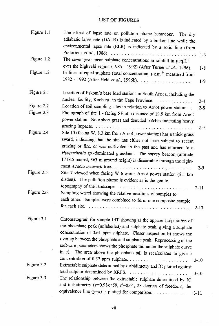
Figure 1.1

Figure 1.2

Figure 1.3

Figure 2.1

Figure 2.2

Figure 2.3

Figure 2.4

Figure 2.5

Figure 2.6

Figure 3.1

Figure 3.2

Figure 3.3

LIST OF FIGURES

The effect of lapse rate on pollution plume behaviour. The dry

adiabatic lapse rate (DALR) is indicated by a broken line while the

environmental lapse rate (ELR) is indicated by a solid line (from

Pretorious et al., 1986) . . . . . . . . . . . . . . . . . . . . . . . . . . . . . . . 1-3

The seven year mean sulphate concentrations in rainfall in µeq.L· 1

over the highveld region (1985 - 1992) (After Turner et al., 1996). 1-8

Isolines of equal sulphate (total concentration, µg.m- 3) measured from

1982 - 1992 (After Held et al., 1996b ). . . . . . . . . . . . . . . . . . . . 1-9

Location of Eskom's base load stations in South Africa, including the

nuclear facility, Koeberg, in the Cape Province. . . . . . . . . . . . . . 2-4

Location of soil sampling sites in relation to Arnot power station. . 2-8

Photograph of site 1 - facing SE at a distance of 19.9 km from Arnot

power station. Note short grass and denuded patches indicating heavy

grazing impacts. . . . . . . . . . . . . . . . . . . . . . . . . . . . . . . . . . . . 2-9

Site 10 (facing W, 8.3 km from Arnot power station) has a thick grass

sward, indicating that the site has either not been subject to recent

grazing or fire, or was cultivated in the past and has returned to a

Hypparhenia sp. -dominated grassland. The survey beacon ( alti~de

1718.5 mamsl, 363 m ground height) is discernible through the right-

most Acacia mearnsii tree. . . . . . . . . . . . . . . . . . . . .. . . . . . . . . 2-9

Site 7 viewed when facing W towards Arnot power station (8.1 km distant). The pollution plume is evident as is the gentle

topography of the landscape. . . . . . . . . . . . . . . . . . . . . . . . . . 2-11

Sampling wheel showing the relative positions of samples to

each other. Samples were combined to form one composite sample

for each site. . . . . . . . . . . . . . . . . . . . . . . . . . . . . . . . . . . . . . 2-13 ·

Chromatogram for sample 14T showing a) the apparent separation of

the phosphate peak (unlabelled) and sulphate peak, giving a sulphate

concentration of 0.61 ppm sulphate. Closer inspection b) shows the

overlap between the phosphate and sulphate peak. Reprocessing of the

software parameters shows the phosphate tail under the sulphate curve

in c). The area above the phosphate tail is recalculated to give a

concentration of 0.57 ppm sulphate. . . . . . . . . . . . . . . . . . . . . . 3-10

Extractable sulphate determined by turbidimetry and IC plotted against

total sulphur determined by XRFS. . . . . . . . . . . . . . . . . . . . . . 3-10

The relationship between the extractable sulphate determined by IC

and turbidimetry (y=0.98x+59, r2=0.64, 28 degrees of freedom); the

equivalence line (y=x) is plotted for comparison. . . . . . . . . . . . . 3-11

vu

Figure 4.1

Figure 4.2

Figure 4.3

Figure 4.4

Figure 4.5

Figure 4.6

Figure 4.7

Figure 4.8

Figure 4.9

Figure 4.10

Figure 4.11

Parameters plotted as a function of distance of sampling from the

Arnot power station a). pH(water), b). water-soluble sulphate c).

phosphate-extractable sulphate and d). total sulphur. . . . . . . . . . . 4-11

Relationship of pH measured in KCI or K2S04 (pHsaiJ to pH measured

in water for the 30 soils . . . . . . . . . . . . . . . . . . . . . . . . . . . . . 4-12

Relationship between pH measured in water and L\pH (i.e. pH(KCl)-

pH( water)) . . . . . . . . . . . . . . . . . . . . . . . . . . . . . . . . . . . . . . 4-13

The relationship between the acid saturation of the effective cation

exchange capacity (ECEC) and pH measured in KCI . . . . . . . . . 4-14

The relationship between acid neutralising capacity (units= cmolc.L-1)

and pH measured in KCI . . . . . . . . . . . . . . . . . . . . . . . . . . . . 4-15

The relationship between difference in pH(K2S04 - KCI) and

phosphate-extractable sulphate . . . . . . . . . . . . . . . . . . . . . . . . 4-17

The relationship between the index of sulphate retention (SRI) and

phosphate-extractable sulphate. . . . . . . . . . . . . . . . . . . . . . . . . 4-18

Phosphate-extractable sulphate as a function of soil organic carbon 4-19

Relationship between water-soluble sulphate and organic C.. . . . . 4-20

Relationship between total S and organic C for the soil collection,

based on data from Tables 4.1 and 4.2. The regression was performed

without the outlier (lOS), giving an r2 of 0.73 (df=27). . . . . . . . . 4-21

Relationship between organic carbon and total sulphur for various parts

of South Africa. Solid lines indicate areas affected ·by atmospheric

pollution. . . . . . . . . . . . . . . . . . . . . . . . . . . . . . . . . . . . . . . . 4-23

Vlll

Table I .I

Table 2.1

Table 2.2

Table 2.3

Table 3.1

Table 3.2

Table 3.3

Table 4.I

Table 4.2

Table 4.3

Table 4.4

Table 4.5

Table 4.6

LIST OF TABLES

Weighted mean composition of bulk precipitation from seven highveld

sites (reported in mg.L-1) (Data from the Hydrological Research

Institute and adapted from Fey and Guy, I993). . . . . . . . . . . . . . I-8

Electricity production and coal consumption for Arnot power station,

together with estimates of sulphur emissions based on the extremes of

sulphur content reported for'South African coals. . . . . . . . . . . . . 2-5

Percentage frequency of occurrence and mean wind speed for each of

the I 6 wind directions at Arnot power station from 1 April 1979 to 31

March I984 (adapted from Pretorius et al., 1986). . . . . . . . . . . . . 2-7

Comparison of selected analytical data for samples taken in August and

October for three sites. . . . . . . . . . . . . . . . . . . . . . . . . . . . . . 2-16

Concentrations of water soluble sulphate in saturated paste extracts

determined by ion chromatography and turbidimetry (mg SO/.L-').

Topsoils are designated by -T and subsoils by -S. . . . . . . . . . . . . 3-5

Phosphate extractable sulphate determined by turbidimetry. Each

analytical run is individually presented to demonstrate the variability

of control soils and blanks between different runs. Topsoils are

designated by -T and subsoils by -S.. . . . . . . . . . . . . . . . . . . . . . 3-6

Concentration of extractable sulphate (mg SO/.kg·' soil) in the soil

collection determined by turbidimetry and ion chromatography (IC).

Topsoils are designated by -T and subsoils by -S. . . . . . . . . . . . . 3-8

Textural, chemical and mineralogical characteristics of the

soil collection . . . . . . . . . . . . . . . . . . . . . . . . . . . . . . . . . . . . . . 4-J Total chemical analysis (major elements) of the soil collection . . . . 4-5

Total chemical analysis (trace elements) of the soil collection . . . . . 4-6

Surface properties (acidity and ion exchange characteristics) of

the soil collection . . . . . . . . . . . . . . . . . . . . . . . . . . . . . . . . . . . 4-8

Solution composition and extractable sulphate in the soil c~llection 4-9

Regression data for soil data sets from different parts of South Africa. .................................... 4-22

ix

INTRODUCTION

Concerns about atmospheric pollution on the South African highveld were raised in the

landmark report by Tyson et al. in 1988. The eastern highveld region is rich in coal seams

which fuel power stations providing 72 % of South Africa's primary energy source. Industries

such as ferro-alloy smelters, petrochemical works and foundries also rely on coal to meet their

energy and raw material requirements. Tyson et al. (1988) highlighted concerns that the

concentration of heavy industry and the unique climate in this region promote the

accumulation of atmospheric pollutants.

Although there may be considerable debate as to the exact mechanisms involved (Sverdrup et

al., 1992) there is little doubt that air pollution from smelters, power stations and other

industries has contributed to the acidification of soils and waters in industrialised regions. In

particular, Scandinavia and Central European countries have borne the brunt of poor

atmospheric pollution control. In the 1920s, the effects of anthropogenic acidification were

first noted in freshwater ecosystems of Southern Norway - where both fish diversity and the

yield of salmonid fishes declined. Although acidification steadily increased it was only in the

period from 1950 to 1980 that large scale deterioration of aquatic environments became

apparent (Brodin and Kuylenstierna, 1992). The decline of coniferous forests in the

mountainous regions of Germany, Poland and Czechoslovakia was believed to be caused by

soil acidification and high airborne concentrations of sulphur dioxide and ozone. Recent forest

health surveys have recorded symptoms such as crown thinning, needle loss, and needle

yellowing in the Nordic countries - symptoms which parallel those found before the

widespread forest decline in Central Europe (Sverdrup et al., 1992).

In South Africa the effects of atmospheric pollution on human health, soils, surface waters,

forests, agricultural crops and the materials used for buildings and other structures have

received research attention (Scholes et al., 1996; Kempster et al., 1996; Fey et al., 1996;

Gnoinski et al., 1996 and Terblanche et al., 1996). It is the European and North American

experience that forested ecosystems are most affected by atmospheric deposition, yet in South

Africa, there is no conclusive evidence of tree damage attributable to atmospheric deposition

(Scholes et al., 1996). Reuss and Johnson (1986) did warn, however, that the effects of

acidification may not be apparent in short- to medium-term experiments, but that long-term

consequences are nevertheless likely.

In Europe, international co-operation to manage atmospheric pollutants has brought about

substantial reductions in the emissions of pollutants such as sulphur dioxide. Although

acidification from S02 is no longer as threatening, other pollutants such as ozone and nitrogen

compounds are receiving greater attention. In addition, there is growing concern over the

impacts which industrial growth in developing countries of the Far East and Africa will have

on environmental resources (Yagishita, 1995; Kuylenstierna et al., 1995).

x

•

The commitment by Eskom, the major electricity generator in South Africa, to produce the

cheapest electricity in the world, has raised the question of how realistic the price of electricity

is, since the wide range of external costs to society have not fully been taken into account.

Van Horen (1996) has attempted to identify some of these costs but often found that

insufficient information hampered his efforts. One such arena where more information was

required was the valuation of the impacts caused by acidification through atmospheric

pollution. At a recent international workshop, the need for further research in South Africa was

considered "of paramount importance if the ecological damage now recognised in North America and Europe is to be avoided" (Bell, 1996).

The power generation industry has a brief history in South Africa and the landscape has

consequently not been exposed to high levels of atmospheric pollution for more than about

thirty years. Indubitably, impacts such as those apparent in the Northern hemisphere are still

possible in South Africa. Acknowledging that time delays in soil responses may be operative,

it would be valuable to establish baseline data against which changes in soil chemistry can be assessed.

The recognition of the need for more information provided the impetus for the current study.

This project seeks to establish a baseline data set against which long-term changes can be

compared. The study site selected is located on grassland so that the acidifying effects of

agricultural harvesting or afforestation are minimal if not. absent. Owing to the prevailing

climatic conditions on the highveld, atmospheric deposition events may be most intense in the

near-field of power stations. The study sites were established along an hypothesized

deposition gradient since spatial comparisons along the gradient may allow some early

inferences to made about possible impacts. Finally, some of the parameters determining the

sulphate retention ability of soil will be investigated.

The broad aims outlined above can be crystallised into four key questions:

Is the sampling of baseline monitoring sites repeatable?

Are the analytical methods employed valid and repeatable ?

Is there an observable soil acidification gradient in the vicinity of an "acid source"?

Does soil sulphur, or some labile fraction of soil sulphate, decrease with distance from a power station ?

By answering some or all of these questions, a start will be made towards assessing the

impacts of atmospheric pollution on the highveld. If no impacts are apparent, the data will in any event constitute baseline information for future studies.

Xl

CHAPTER 1

AIR POLLUTION IMPACTS ON SOIL CHEMICAL PROPERTIES - A

LITERATURE REVIEW

1.1 Introduction

The deposition of air pollutants on the soil gives cause for concern because of the possible

impact on agricultural productivity and water quality. The eastern highveld was identified by

Tyson et al. (1988) as an area of special concern because of the combination of heavy industry

and climatic conditions which promote the accumulation of atmospheric pollutants. The fate

of these pollutants rests on atmospheric processes which will determine whether the pollutants

are dispersed or deposited. The link between atmosphere and pedosphere is therefore the focus

of this chapter.

1.2 The climate of the southern sub-continent

The emission of primary industrial pollutants is relatively constant throughout the year.

Consequently it is the meteorological conditions in the region that control the concentration

of secondary pollutants such as sulphate. Parameters such as temperature, humidity, hours of

sunshine and wind are all determinants of secondary pollutant formation, transportation and

dispersion -(Held et al., 1996a). Some background information on key climate factors will be

presented in order to facilitate an understanding of the potential extent and impacts of air

pollution in the highveld region.

1.2.1 General atmospheric circulation

An anticyclone is a syst,em of winds rotating outwards from an area of high barometric

pressure which results in fine stable weather. In general, the atmospheric circulation over southern Africa is anticyclonic above 700 hPa. The frequency of the anticylonic circulations

reaches a maximum in the winter - occurring on 65 % of days or more. The stable conditions

·that prevail during an anticyclone allow large-scale elevated temperature inversions to form

which prevent the vertical dispersion of pollutants. Inversions play an important role in pollutant dispersion and therefore warrant some further discussion.

1-1

1.2.2 The development of temperature inversions

Convection lowers the temperature of the earth's surface because a parcel of warm air at the

surface will rise, carrying heat away from the surface. As the parcel rises, it expands and the

work done causes it to cool adiabatically, i.e. there is no exchange of energy with the outside

air. For the atmosphere of the earth, the lapse rate is calculated as - 9.8 K.km-1 for dry air.

However, the measured rate is - 6.5 K.km-1 because air bears moisture which condenses as it

rises and releases latent heat (Brimblecombe, 1986).

If the actual change in temperature in the ambient air is greater than the lapse rate, then a

rising air parcel is at a higher temperature than the surrounding air. The parcel will have a

greater tendency to rise and causes "unstable conditions" because convective mixing takes

place. Under neutral conditions, the environmental lapse rate is similar to that expected under

adiabatic expansion. If the environment cools less rapidly with height than the adiabatic lapse

rate, then an "inversion" has formed. Radiation inversions form at night when the ground

cools more rapidly than the air, but may break up during the day when the sun warms the

ground (Brimblecombe, 1986).

Elevated inversions are caused either by the subsidence of an air mass or by the frontal

movement of air masses. According to Held et al. (1996b ), the base heights of these

inversions on the South African highveld are at 1 700 m above ground level in the winter but

in summer can range from 2 000 to 3 000 m above ground level. In the summer months,

cyclonic circulations occur at the 850 hPa level allowing troughs to develop over the central

plateau of the country which destroy the inversions. In the winter months, the stable

anticyclonic conditions also allow surface-based inversions to develop at night. On the

highveld, surface-based inversions can range in strength from 3 to I I °C and in depth from less

than I 00 m to 400 m above ground level. The surface inversion depths in summer are similar

to those in winter but rarely exceed 2 °C in strength. These inversions create a stable

boundary ~ayer which prevents the dispersion of low level emissions. Nocturnal inversions

occur with a frequency of 80 - 90 % during the highveld winter, and so exert a strong

influence on pollutant dispersion. However, a nocturnal low level wind maximum, known as

a Low-Level-Jet (LLJ) often develops above the surface inversions. It forms under highly

stable nocturnal conditions, with speeds ranging from 5 - I5.5 m.s·1, and serves as an efficient

dispersant in the first few hundred metres above ground level (Held et al., I996[>).

1.2.3 Atmospheric stability and pollutant plume behaviour

The stability of the atmosphere determines pollutant plume behaviour and dispersion

characteristics (Figure I. I). Under unstable conditions, the pollution plume may loop violently

when it encounters strong convective eddies. High ground-level concentrations of pollutants then result. Turner (I 996) reports that although the typical position for maximum plume

1-2

impact is about ten stack lengths downwind of tbe source, plume strikes have been recorded

within two stack heights of the source. Fumigating plumes, which occur when the air is stable

above the emission point also result, in high concentrations of pollutant at ground level.

Coning occurs under near-neutral conditions and leads to equal dispersion in the horizontal and

vertical directions. Fanning occurs in very stable conditions, such as an inversion, leading to

much horizontal dispersion but little vertical dispersion. Lofting occurs when the emission is

just above an inversion layer and disperses pollutants both vertically and horizontally (Held et al., l 996b; Brimblecombe, 1986).

Figure 1.1

(a)

TEMPERATURE -STRONG LAPSE CONOITJON (LOOPING I

TEMPERATURE -

. 11

~

1 WEAK LAPSE

. (c) ~ ,~ I, ...... ____ '"'"=.....,_ .... -="-- •

CONDITION ( CDNINGf

TEM!>E:RATURE -INVERSION CONDITJOH IFAlfNINGI

TEMPERATURE INVERSION BELOW, LAPSE ALOFT (LOFTING)

TEMPERATURE -LAPSE BELOW, INVERSION ALOFT (FUMIGATION-I

t ' (fl~ \ ..,,...~"'7-:=~;:.::-.,~,·;;--i-))-_; :-

= ' ~--"'-'-' .·.J - -· •• ·- --w \ ~~ .. -- ........... -:: ' ~¥~j~

TEMPERATURE -Wf:AJC LAPSE 8EL01!1, INVERSION ALOFT (TRAPPING)

The effect of lapse rate on pollution plume behaviour. The dry adiabatic

lapse rate (DALR) is indicated by a broken line while the environmental

lapse rate (ELR) is indicated by a solid line (from Pretorious et al., 1986).

The plumes from the Eskom power stations are reported as amongst the most bouyant in the

world (Turner, 1996). Such buoyant plumes are generally able to break through the stable

boundary layer that develops at night and are dispersed in the overlying neutral layer or are

carried off by the LLJ. The boundary layer prevents the plumes from mixing down to ground

1-3

level. During the day, however, the convective boundary layer encourages strong looping

behaviour which results in high pollutant concentrations near to the plume source. Modelling

of plume behaviour under such extremes of stability and instability is difficult - particularly because the peak concentrations often occur when the mean wind velocities are low.

1.3 Atmospheric deposition

Wind-entrained dust, smoke from biomass burning, marine salts and air pollutants all

contribute to atmospheric deposition. Although a variety of compounds are deposited on the

soil surface, it is the acidifying compounds, trace elements and heavy metals derived from industrial processes which generally cause environmental damage.

Apart from the impacts associated with the gaseous compounds of N and S, power station

emissions in South Africa are unlikely to cause any serious pollution problems. Compared with

coals from the United States, Australia, Belgium and Germany, South African coal was found

to be generally low in trace elements such as Pb, As, Zn and Ni (Willis, 1983; Willis, 1987).

Sulphuric, nitric, carbonic, hydrochloric, phosphoric or organic acids may all enter an

ecosystem through atmospheric deposition processes. Of these, sulphuric and nitric acids are

the most common anthropogenic acids and the ones which give the most cause for concern.

Nitrogen is often limiting as a plant nutrient and its deposition as nitric acid serves to fertilize

ecosystems that are N-poor. The biological interactions involving N are quite complex and

beyond the scope of this review. For discussion of nitrogen transformations as acidifying processes, I refer the reader to Reuss and Johnson (1986).

Although South African coal is low in S (0.4 - 1.6 %) compared with coals from Europe

(Willis, 1983), S emissions are significant because of the large quantities of coal that are burnt

annually on the South African highveld, both for industrial purposes and as a domestic fuel

source. In the past, the burning of coal discard dumps was a substantial source of low level

emissions of sulphur dioxide although such sources are now largely controlled (Wells et al., 1996).

1.4 Atmospheric deposition processes

Three processes of atmospheric deposition can be distinguished. Wet deposition occurs in precipitation - generally rainfall or snowfall. In dry deposition processes, gaseous and

particulate matter is directly deposited from the atmosphere to the surface. Mist deposition is usually treated separately because the surface is exposed for long time periods and to

relatively concentrated solutions. The semi-arid climate of the South African highveld,

compared with many similarly affected northern hemisphere landscapes, means that wet

1-4

deposition is not the predominant means of pollutant deposition. Close to the pollutant source,

dry deposition is most likely dominated by gaseous components whereas further from the

source aerosols will dominate (Held et al., l 996a).

The measurement of dry deposition is both difficult and expensive and very little work has

consequently been done on this aspect in South Africa. Nevertheless, the flux of acid

pollutants to the surface by dry deposition either equals or exceeds that by wet deposition. Dry deposition is calculated as follows:

Flux to surface (Q) = vdc

where

and C = concentration of species (gas molecule/particle/aerosol) in the air

V d = deposition velocity - which depends on factors such as time of day,

surface chemistry, surface moisture and vegetation type.

The measurement of dry deposition is presently receiving much attention in the highveld

region especially since estimates range from the same magnitude as wet deposition to six times as much (Turner et al., 1996).

Deposition through mist is generally more acidic than rainfall, and contains higher

concentrations of dissolved chemical species. For example, a study by Olbrich (1993) found

that mist samples contained almost double the sulphate concentration than rain. Since mists

are generally of greater duration, they can potentially have greater impacts - especially 1n forested areas. However, except for on the Drakensberg escarpment, and high lying areas near

Dullstroom, mist events are rare on the highveld.

1.5 Emission, conversion and deposition of sulphur compounds

1.5.1 Sulphur dioxide

Sulphur dioxide is a primary pollutant emitted directly from sources such as coal-fired power

stations, biomass burning, and industries such as ferro-alloy works, steelworks and foundries.

Estimates of temporal variation in S02 concentrations depend on the sources being considered.

On a seasonal basis, domestic space heating coupled with lower mixing heights of the

boundary layer contribute to elevated S02 levels in the winter months. On the other hand

sulphur dioxide derived from power stations is emitted at a relatively constant rate. The

concentrations of S02 due to low level sources are greatest at night because of nocturnal

inversions whereas daytime atmospheric mixing and advection have the capacity to disperse

S02 accumulations from the previous night. Thus multi-day accumulations of S02

near ground-level do not occur (Annegam et al., 19.96)..

1-5

Turner (1990 - cited in Annegarn et al., 1996), summarised the findings of a five year study

conducted in the industrial highveld region. He found that the concentrations of S02 in both

rural and urban areas of the highveld seldom exceeded the 24-hour average guideline of

I 00 ppb set by the Department of Environmental Affairs and Tourism. At most monitoring

sites the guideline values were not even approached while the monthly and yearly guideline

values were never exceeded. Annegam et al. (1996) concluded that the ground level

concentrations of sulphur dioxide are adequately controlled and did not _pose a threat to either

human health or the environment. However; they did make an exception for areas close to ·

tall stacks (within a 4 km radius) because the plumes may reach ground level under conditions

of turbulent convective mixing, resulting in peak concentrations close to elevated sources.

Thus, under circumstances of atmospheric turbulence, dry deposition of sulphur dioxide may

be quite considerable in the near-fields of power stations and similar industrial plants.

There is a clear gradient of both decreasing concentration and decreasing frequency of

short term high S02 concentrations from the industrialised part of the Mpumalanga highveld.

Regional air recirculation is also suggested to result in widespread episodes of high pollution

concentrations. This hypothesis was tested using the existing S02 data set maintained by

Eskom1• However, no inter-site correlations between daily mean S02 concentrations were

found. Annegam et al. (1996) concluded that neither pollution episodes.caused by stagnation

nor the recirculation of air occurred regularly in the region. Alternatively, if such episodes

do occur, then the episodes are of short duration.

1.5.2 Transformation of sulphur dioxide to secondary pollutants

Factors such as sunlight, atmospheric oxidation and interactions between different pollutants

drive the formation of secondary pollutants from sulphur dioxide. Ultimately, the atmospheric

conversion rates will largely dictate in what form the pollutant is deposited (Held et al., 1996a). Four main processes have been defined by Pienaar and Helas (1996a,b), which may

be summarised as :

Gas-phase reactions: Although the oxidation of S02 to S03 is thermodynamically

favourable, the reaction is so slow that it can be ignored (about 5% per hour in summer).

However, if S03 is formed in the presence of a catalyst, it then reacts immediately with

water vapour to form sulphuric acid (H2S04).

Photo-oxidation reactions: The photo-oxidation of S02 is considered to be unimportant

in the troposphere. Although the reaction of hydroxyl radicals with S02 is the main

oxidation process, it is very slow. The 24-hour averaged rate of S02 oxidation is

estimated at 0. 7 % per hour under cloudless summer conditions in a fairly clean

Eskom is the major electricity generator in South Africa.

1-6

atmosphere. The resultant series of chemical reactions that gives rise to H2S0

4 is thus

limited by the slow oxidation rate.

Heterogeneous processes: Although particles of fly ash, ferric oxide, dust and soot are

reported to enhance the oxidation of S02 (Saxena et al. 1995), the work of Pienaar and Helas (1996a) did not find this to be the case.

Aqueous phase processes: In polluted atmospheres, aqueous phase reactions are the

major contributors to atmospheric acidification. Tropospheric pollutants such as ozone,

H20 2, peroxyacetyl nitrate (PAN) and peroxyacetic ac!d dissolve in cloud water and then

readily oxidise dissolved S02• In the gas-phase such reactions do not occur at

measurable rates. The rates of aqueous phase oxidation depend on the gas-phase

concentrations, solubility and rate of mass transfer of the oxidising agents such as ozone.

hydrogen peroxide and the hydroxyl and peroxyl radicals (Pienaar and Helas, 1996b).

Despite the various reaction pathways, most of the sulphur deposited on the soil surface will

ultimately form H2S04• Even if subject to various delays because of biological

transformations, Reuss and Johnson (1986) assume that most sulphur will reach the soil

solution within the same annual cycle in which it was deposited. However, this assumption

might be questionable in the less humid climate of South Africa. Nevertheless, whether

deposited directly in the gas phase or following conversion to the particulate phase, sulphur dioxide is an acidifying compound (Annegarn et al., 1996).

1.5.3 Dispersion and deposition of sulphate

The mean rainfall composition for seven highveld sites is presented in Table 1.1. Rainfall in

equilibrium with atmospheric C02 has a pH of 5.6 (Galloway et al., 1976) thus the mean pH

of 4.9 reported for rainfall on the highveld is not unduly acidic. Rainfall in industrialised

regions can be less acidic than anticipated because of neutralisation by base cations. Base

cations may originate from industrial processes, dust from unpaved roads or tillage practices,

or wind erosion (Hedin et al., 1994; Schlesinger, 1991). The inputs of base cations in

deposition, whether from soil dust or from industrial emissions, is an aspect that has received very little attention, and one which Kuylenstiema (1996) believes could be significant in South Africa.

1-7

Table I. I Weighted mean composition of bulk precipitation from seven highveld sites

(reported in mg.L-') (Data from the Hydrological Research Institute and adapted

from Fey and Guy, 1993).

Cations Anions

Na+ 0.72 p· 0.08 Mg2+ 0.30 c1· 0.97 Ca2+ l.15 sot 2.89 NH

4+ 0.65 PO/" 0.09

K+ 0.40 No 2• J 0.51 Si4+ 0.25 Total alkalinity 5.07

pH 4.94

Long term monitoring has shown sulphate to be the most abundant anion in rainfall - whether

in the industrial highveld region or the more rural Northern province. Figure 1.2 shows the

seven year mean sulphate concentrations over the highveld area and these are comparable to

those reported for similar regions in the United States. However, the central highveld receives

less rain (between 600 - 700 mm per year), so that typical annual deposition loads in rainfall

are estimated at 17kg S04 2·.ha·1 on the central highveld, which is approximately half of the

maximum load reported for the US (Turnet et al., 1996). Inputs of sulphate through dry

deposition have not been included in either the US or South African estimate. As mentioned

earlier, estimates of dry deposition range from being equal to wet deposition to six times as

much.

Figure 1.2

2s•

~29"~~--/ . .. . .Louis.Trichatd! (18) \

,.,.., • ········r···

Pielersburg o

Pretoria• Wilbank

Johannesburg o

~.-

I I \1 \

• .. \ I ;~·I

/ I / o Mbabane !

\AnwstOOtt/I I

The seven year mean sulphate concentrations in rainfall in µeq.L·' over the

·highveld region (1985 - 1992) (After Turner et a/., 1996).

1-8

Sulphate concentrations collected from mist samplers located In tbe escarpment region were

found to be almost double those for rainfall (Olbrich, 1993). Deposition through this

mechanism is restricted largely to the escarpment regions of the highveld and would rely

heavily on canopy interception.

The dry deposition of sulphate aerosols was monitored over seven years on the highveld and

mean concentrations of particulate sulphate were found to be 1ow and fair1y evenly distributed

(Figure 1.3). Such distribution is accounted for by the uniform distribution of sources of 802

and the slow conversion and deposition rates of sulphate.

Figure L3

2re 28 E 29'E 30°E .

I .·". Pr~toria ... ·; ·· .... · l···· ....... · ... .J ,.....,.,.---'-----f--~· 26'5

---Jo-~-an.,_,__~-esbur~. ~ j / "· ...

1 h : ,r-?: 3

0

_.='--'-------~ ~

... l . . . .. . I I ······L ·1

i .... . . . .. . ...... 1 . 1'

... --· .. ·· ..... ··~ ·-- I . 4_ 28"

Isolines of equal sulphate (total concentration, µg.n{') measured from 1982 -

1992 (After Held et al., 1996b).

·Most monitoring sites recorded concentrations between 3 and 5 µg.m·3• The crucial factors

defining the concentrations of sulphate on the highveld were the type of air mass, the pressure

system determining the intensity and direction of the air mass flow, the depth of the mixing

layer and the oxidation chemistry (Held et al., 1996b). The sulphate aerosol is reasonably well

correlated with temperature and humidity but not with wind speed. In the warmer months the

movement of moist, warm air masses over the sub-continent results in higher st1\phat-e

concentrations. Thus suTp'hate concentrations are higher in summer and lower during winter,

altbough tliis general trend is overlain by high sulphate episodes throughout the year.

At high elevations (above 300 m above ground level) sulphate concentrations are higher - for

example 71 µg.m·3 was recorded at the top of Verkykkop and 51 µg.m·3 at the top of the

Kendal power station stack (before Kendal came into operation) (Held et al., 1996a). Such

high concentrations occur either because of accumulation of particulates at higher altitudes or

because of recirculation of air masses on a regional scale. Aerosol layering in the middle

troposphere has recently been confirmed by the study by Held et al. (1996c)~

1-9

Episodes of high sulphate aerosol concentrations at ground level can occur when the postulated

pool of pollutants at higher altitudes is mixed down towards the surface. At ground level, the

highest sulphate concentrations seldom exceeded the 25 µg.m-3 limit laid down by the

California Air Resources Board. Held et al. (1996b) estimated that such episodes occur on

average 19 times per year and each lasts a few days. Episodes of low sulphate concentrations

occur, on average, 17 times per year, also lasting a few days.

The tall stack policy adopted by Eskom appears to have controlled the ground level

concentrations of both primary and secondary pollutants. However, this policy, together with

the local meteorological conditions, has brought about high concentrations of secondary

pollutants, such as sulphate aerosols, at elevated layers (Held et al., 1996a; Held et al., 1996c).

1.6 Impacts of atmospheric deposition on soil

Acid deposition acts to increase the exchangeable acidity of soil and reduces the fraction of

exchangeable bases (Koptsik and Mukhina, 1995). The exchangeable acidity is either directly

increased through the inputs of H+ or by the increase in exchangeable aluminium through the

reaction of H+ with soil minerals. The aluminium species replace the base cations on the soil

exchange complex and the base cations are then leached from the system in tandem with

strong acid anions such as sulphate (Reuss and Johnson, 1986).

According to Reuss and Johnson (1986), sulphate leaving a system must be accompanied by

an equivalent amount of cations because of charge balance considerations. The export of the

base cations will tend to acidify the system, although the time scale over which acidification

will occur is strongly dependent on the nature of the soil affected. In alkaline or neutral soils,

the negative exchange surface is dominated by the basic cations (Ca2+, Mg2+, Na+ and K+)

whereas H+ is the dominant exchangeable cation in organic acid soils. Aluminium species,

such as AI3+, Al(OH)2+ and Al(OH)2 + which have formed from the dissolution of soil minerals,

dominate in acid mineral soils. In strongly acid soils, the high levels of aluminium that may

result may be toxic to plants although susceptibility will depend on the plant species, and the

composition of the soil solution.

The effects of increased proton loading on the vast range of heterotrophic soil organisms,

particularly the microbial population, are poorly understood (Wolters and Shaefer, 1994). The

effects on soil biota may be caused directly through proton toxicity or indirectly, through

factors such as nutrient imbalances, mobilization of toxic metals or changes in the structural

habitat of the soil. Processes like humification and nitrogen fixation could be halted at low

pH values and rates of litter decomposition could also change. Changes in the community of

soil organisms can affect chemical and nutritional properties or soil structure and texture, and,

ultimately these changes could affect both the structure and functioning of terrestrial ecosystems.

1-10

The deposition of sulphur compounds from the atmosphere also results in an increase in the

concentration of sulphate in the soil solution. Concerns that sulphate d~position may be

increasing the solute load in runoff and thereby salinizing the major water supply of Gauteng

prompted a one-year study of the soils of the Vaal Dam catchment (Fey and Guy, 1993). On

average, the soils of the V aal catchment had double the concentration of sulphate in solution

found for comparable soils from southern Natal. Skoroszewski (1995), in another short term

study, measured sulphate outputs from a small catchment in the Suikerbosrand Nature Reserve,

near Johannesburg, and the results suggested that between 9 and 17 % of the measured

sulphate inputs through deposition were being retained in the soils. The remaining sulphate

was beincg removed in surface runoff.

According to Reuss and Johnson ( 1986), the response of the soil solution to increased sulphur

inputs will depend on factors such as biological uptake and the ability of many soils to retain

sulphate on soil surfaces. Although sulphur is an essential plant nutrient, the plant

requirements for sulphur are soon met. Thus sulphate retention on soil surfaces, particularly

sesquioxides, is an important buffer mechanism in the soil. In this way, the secondary effects

of acid deposition - such as base cation removal, aluminium mobilization and decreased

alkalinity of the soil solution - may be delayed by years or even decades.

' It must be stressed that the acidification of soil is a natural process in many systems -

particularly in humid climates where water accelerates reactions (McBride, 1994). In systems

unaffected by acid deposition, base cations are leached out in association with organic acids

or bicarbonate (HC03·). The net accumulation of basic cations into the biomass also acidifies

the soil over time. In natural systems the base cations will ultimately- be returned to the soil

via the processes of decomposition but where biomass is harvested, the base cations are

exported and then can only be replaced through mineral weathering or artificial fertilizers

(Reuss and Johnson, 1986; McBride, 1994).

McBride (1994) cites two other mechanisms of natural acidification: the oxidation of sulphides '

in soils with fluctuating water tables, and nitrogen transformations such as nitrification. In

both processes, the time scale at which the system is considered is important since the

acidification may be reversed once the reducing conditions return or the denitrifying bacteria

are activated.

In view of its importance in mediating the impacts of sulphate-laden pollution on soil chemical

properties, sulphate retention by soil will form the focus of the remainder of this review.

1-11

1. 7 Sulphate sorption in soil

Isomorphous substitution of ions in clay lattices (such as Mg2+ for A13+, and Al3+ for Si4+), is

primarily responsible for the net negative charge carried by most soil surfaces (Alloway,

1995). However, positively-charged sites may exist within a soil having a net negative charge

(McBride, 1994). This obviously has important implications for the sorption of sulphate as

an anionic species. Before exploring how positively charged surfaces arise in soils, it is useful

to consider the interaction between the soil surface and soil solution in a little more detail.

In the simplest view, the negative charge on the clay minerals is smeared out over the planar

surfaces of the crystals (White, 1979; Wild, 1993). Each surface charge is neutralised by a

mobile ion of opposite charge to give an alignment of charges in two planes which is termed

a Helmholtz double layer .. However, the spatial distribution of the ions is dictated by two

opposing forces: i) a diffusive force which drives the mobile cations away from the high

concentration near the negatively-charged clay surface to the outer solution, and ii) the

electrostatic forces attracting the cations towards the charged surface. The result is a diffuse

distribution of cations and anions in solution which, together with the surface charge, is termed

the Gouy layer.

A more realistic model of charge distribution is represented by the Stem model which

combines the concepts of the Helmholtz and Gouy models (White, 1979). The Stem model

· .·. can accommodate ions of greater valency, does not regard the ions as point charges and,

importantly, recognises other forces between the ions and the mineral surface beside simple

electrostatic attraction. Essentially, the solution component of the double layer is split into

two components: i) The Stem layer, which is a plane of cations of finite size located close

to the clay's negative surface. In this region the electrical potential decays in a linear fashion

with distance from the clay surface. ii) The diffuse layer of cations, across which there is an

exponential decrease in the electrical potential. The inner surface of the diffuse layer contacts the Stem layer and is termed the outer Helmholtz plane (White, 1979).

1. 7.1 Positively charged soil surfaces

Positive sites on a soil surface are accounted for by the uptake of protons from solution on to

suitable sites - particularly under acidic conditions - when NH2 and OH groups are protonated

to NH3 + and OH2 + (Mott, 1981; White, 1979). Sulphate sorption by soils is strongly pH­

dependent, especially when dealing with variably charged soils which can reversibly adsorb

H" ions. The sites of pH-dependent charge are responsible for most of the positive charge present in soils.

1-12

The sulphate anion interacts with soil minerals which possess these surface hydroxyl groups.

Such minerals include the poorly crystalline aluminosilicates (allophanes), the oxides of Fe,

Al and Mn and the edge sites of the layer silicate clays (McBride, 1994). Kaolinite has been

identified as an effective adsorbent for aqueous sot (Kooner et al., 1995; Mott, 1981).

Although sulphate is highly desorbable from kaolinite, this is not the case for desorption from

hydrous oxides of Fe and Al (Mott, 1981). Quartz lacks Al and Fe exchange sites on the

mineral surface and so has low SOt sorption capacity (Li.ikewille et al., 1995)..

1. 7.2 Adsorption

Ions in the diffuse layer (sometimes referred to as the diffuse ion swarm) are free to move

about in the soil solution and are fully dissociated from surface functional group_s (Sposito,

1989). The soil surface charge is neutralised only in a deloc.alised sense, by simple

electrostatic attraction. There is no electron transfer or sharing between ion and crystal

(Sposito, .1989; Mott, 1981). The monovalent anions, c1· and N03·, are non-specifically

adsorbed anions forming part of the diffuse-ion swarm. Another type of electrostatic bonding

which has been recognised, is termed "outer-sphere surface complexation", in which at least

one water molecule is interposed between the positive surface group and the complexed anion.

Both diffuse ion association and outer-sphere complexation can be described as non-specific

adsorption. Sposito (1989) considers that the S042• anion adsorbs mainly as a part of the

diffuse-ion swarm and as an outer-sphere complex species. His conclusion is based on the

observed readily exchangeable character of the anion and is supported by several subsequent

studies cited by Gustafsson (1995).

Specific adsorption corresponds to what is sometimes termed inner-sphere surface

complexation, which may involve ionic as well as covalent bonding (Sposito, 1989).

According to Mott ( 1981 ), the sulphate ion falls into the class of specifically adsorbed anions

which are adsorbed by chemical bonding at specific sites to form a ligand. Most often the

mechanism for this coordination is ligand exchange for hydroxl ions. Such adsm;ption is

termed "chemisorption" and is often thought of as being irreversible. McBride {1994) lists

four criteria for recognising ligand exchange or chemismption:

i) The release of Off into solution;

ii) A high degree of specificity of the surface towards particular anions;

iii) The reaction is non-reversible, or desorption is considerably slower than

adsorption;

iv) A change in the measured surface charge to a more negative value followip.g

adsorption.

Most studies have concluded that SO/" is a specifically adsorbed(chemisorbed) anion (studies

. cited in Zhang et al., 1987 and in Guadalix and Pardo, 1991 ). Evidence for this is provided

1-13

'"

by the fact that SO/ displaces Off in a ligand exchange-type reaction which results in the

release of Off ions to the soil solution, and a subsequent increase in solution pH. Thus the

pH of soils equilibrated with SO/ is higher than that of soils equilibrated with c1- or No3-,

since these latter ions are adsorbed without the release of Off ions. The increase in cation

adsorption which results is due to the net increase of surface negative charge associated with sulphate adsorption (Curtin and Syers, 1990a).

Adsorption of SO/ is typically found to increase with a decrease in pH (Zhang et al., 1987; ',

Kooner et al., 1995). According to the latter a1;1thors, the adsorption of sot is restricted to

the positive side of the zero point of charge, via either inner- or outer-sphere adsorption

mechanisms, so that SO/ adsorbs primarily to those mineral surface sites which are positive

or neutral. The adsorption of SO/on oxide surfaces results in the release of OH- and/or H20

ligands (Inskeep, 1989). Having displaced the Off and OH2 ligands , the sot is then

adsorbed to either one or two Al or Fe atoms. Kooner et al. (1995) refer to these mechanisms

of sot adsorption as monodentate - or bidentate inner-sphere complexes, respectively. The

bidentate inner-sphere complexes are supposedly less stable than the monodentate inner-sphere

complexes, because each sulphur atom is shared between two surface sites which places a

strain on the bonds with the surface (Kooner et al., 1995). On the other hand, McBride

(1994), who terms such adsorption a "binuclear bridging mechanism" states that adsorption

, ~ould be non-reversible, since desorption would require two bonds to be broken

simultaneously.

In studies of this type it is important to consider the solution pH at which the adsorption

process occurs. At low pH, the OH ligands would be protonated to OH2, which, when

replaced by the sulphate ligand, is simply given off as water and would not reflect an increase

in pH. Thus, Zhang et al. (1987) found that the ratio of Off released to SO/ adsorbed was

very low at pH 5.

Numerous studies have shown SO/ adsorption to be fully reversible (studies cited in Freney

and Williams, 1983; Novak and Pfechova, 1995). This suggests that the adsorption of SO/

does not meet the criteria set by McBride (1994) that chemisorption be non-reversible or have

a slower rate of desorption than adsorption.

Mott ( 1981) describes low-affinity specific adsorption for those ions which are attracted to a

surface to a greater extent than would be expected from diffuse layer theory, yet are not bound to the surface. Curtin and Syers (1990a) have used this idea to explain how sot was

quantitatively removed by extraction with an indifferent electrolyte solution. They reasoned

that if SO/ is chemically bonded to surface metal atoms, then it is unlikely that adsorbed

SO/ would be completely removed by an indifferent electrolyte such as NaCL Since the SO/ could be extracted, it was suggested that the SO/ is adsorbed in a plane closer to the

surface than are monovalent ions (which are attracted purely by electrostatic forces) but is not

chemically bound to the metal surface. Instead, it was proposed that the S04 2- is adsorbed into

1-14

' the Stem layer, where further positive charge is induced on the surface by OH- release.

Adsorption of SO/- into the Stem layer diminishes the capacity of the diffuse layer to hold

anions electrostatically, while cations are held in larger numbers. This type of interaction has

been termed "low-affinity specific adsorption" to distinguish it from chemisorption.

Accordingly, although the forces involved will be other than purely electrostatic, SO/- does

not become chemically ~o-ordinated to the surface metal atoms as do chemisorbed anions such

as phosphate (Curtin and Syers, 1990b).

1. 7.3 Precipitation reactions

Some studies have suggested that SO/ retention by soils is inadequately explained by

adsorption alone. An alternative mechanism involves the precipitation of aluminium sulphate

minerals such as jurbanite (AlOHS04.5H20), alunite (KAlJ(S04)z(OH)6) and basaluminite

(All0H10)S04.5H20) (Liikewille et al., 1995; Fey and Guy, 1993; Sposito, 1989). Formation

of aluminium sulphate minerals is possible in high sulphate, low pH environments where the

resultant minerals are more stable than existing aluminium solids such as gibbsite and kaolinite

(Fey and Guy, 1993). The low pH is necessary to ensure that there is sufficient Al in solution

to enable the precipitation reactions to proceed (Sposito, 1989; Liikewille et al., 1995).

Although the precipitation of such minerals is supported by solubility data, no direct evidence

for their formation has yet been presented, except in special cases such as acid sulphate soils

(Curtin and Syers, l 990a). Recent attempts at modelling sulphate sorption and desorption in

soils have either been based on adsorption isotherms or have incorporated the chemical

equilibria of these minerals. The studies by Liikewille et al. (1995) and Alewell et al. (1995)

found that ~e data were more accurately described by a model based on the Langmuir

isotherm than one based on the solubility products of jurbanite, and alunite.

On the other hand, in a similar attempt to model SO/- sorption and desorption, Prenzel and

Meiwes (1994) found that their results could not be adequately described by adsorption

isotherm models. A model based on the solubility product of jurbanite (Al0HS04) was more

successful in describing the soil solution data. The authors were careful to point out that the

appropriateness of their model did not prove the formation of the aluminium suJphat-e

minerals in the soil. Rather, they viewed the use of solubility equilibria as an appropriate

basis for explaining the interaction between the soil solution and soil surface.

From the above discussion it is evident that the retention of sulphate on soil surfaces is not

amenable to simple description. Sulphate does not always behave a~ a conventional,

specifically adsorbed anion, since sorption is apparently reversible on kaolinites but not oxides.

Several studies have been cited which imply that the sulphate does not reach the inner

Helmholtz p1ane and so is not involved in ligand exchange or chemisorption. Yet, the anion

is clearly attracted more readily to the surface than an electrostatically bound ion such as er.

1-15

In summary, Mott (1981) describes sulphate as "in some ways the most puzzling of all the anions with respect to sorption".

1. 7.4 Factors influencing sulphate sorption

The soil properties most commonly correlated with sot sorption are pH, ionic strength,

extractable Fe and Al, organic matter and clay content, although the relationships between

these properties and SO/ sorption~are not necessarily simple, linear functions. Adsorption

of sulphate is negligible above pH 6.5 and increases with decreasing pH below this value

(Tabatabai, 1982). Bolan et al. (1986) found that sulphate sorption always decreased with

increasing solution ionic strength. The importance of one soil property over another in

dictating sorption behaviour will also vary between different soils (Comfort et al., 1992).

Ligand exchange of sot for OH" or H20 occurs at the surfaces of Fe or Al oxides or

kaolinite - depending on the surface charge of the edge sites. Of these, Tabatabai (1982)

considers Al to be the most important in sulphate adsorption. The adsorption of sulphate by

different constituents occurs at a number of energetically different reaction sites.

The amount of sorbed SO/- is negatively correlated with the organic matter content of the soil

because of the competition between sot and organic anions for Al binding sites on soil

minerals and oxides (Comfort et al., 1992; Inskeep, 1989, Kooner et al., 1995; Courchesne

et al., 1995; Guggenberger and Zech, 1992). Liikewille et al. (1995) found less sorption in

upper soil horizons and attributed this to a higher organic matter content. Organic acids

containing carboxylic or phenolic functional groups can bind to oxide surfaces, thereby

reducing the amount of surface sites available for anions such as SO/. Inskeep (1989)

stresses that it is the quantity of functional groups available for surface binding that is

important, rather than the amount of total carbon present. An experiment on a podsolic soil

showed that the efficiency of organic matter in displacing sot is controlled by the extent of

proton dissociation from the functional groups of the organic matter. The dissociation of

acidic groups should increase from pH 3.2 to pH 4.2, thus increasing the net negative charge

ofhumic acid molecules and enabling them to compete with S042- for positively charged sites

(Courchesne et al., 1995).

1. 7.5 Kinetic aspects of sulphate sorption

The release of OH· from the soil provides a useful basis for estimating the rate of adsorption

of SO/-. Zhang et al. (1987) found that adsorption proceeded rapidly - with approximately

80 % of the total displaced OH" being released within 4 minutes. Similar results were reported

by Bolan et al. (1986, cited in Novak and Pfechova, 1995) and Rajan (1978, cited in Inskeep,

1989). On the other hand, the study by Kooner et al. ( 1995) found that the adsorption of

sot was a time-dependent process which only reached equilibrium within 4 days.

1-16

The soils used by Zhang et al (I 987) were described as predominantly kaolinitic whereas those

of Kooner et al. (1995) contained appreciable quantities of Fe and Mn oxides in addition to

kaolinite. These differences could account for the marked differences in sulphate sorption

rates, with sulphate being sorbed fastest on the kaolinite soil. However, this explanation

contradicts the earlier finding that sulphate adsorption on Al and Fe oxides is instantaneous

(Novak and Prechova, 1995). Tabatabai (1982) also mentions that sulphate sorption on

kaolinite is weak relative to that on Fe and Al oxides.

Broad comparisons of this nature should be made with caution since different experimental ·

protocols, soil types and analytical methods may conspire to produce an apparently confusing

picture. Nevertheless, present evidence would suggest that different mechanisms may operate

on different mineral surfaces in the soil for the retention of sulphate. This idea was mentioned

earlier by Mott ( 1981 ), when pointing out the discrepancies in adsorption/desorption behaviour

in oxides and kaolinites.

Recent studies have shown that atmospheric sot deposition in Europe has decreased, with

the result that concentration of SO/ in soil solutions and runoff has also decreased. _However,

the observed rate of SO/ decrease in soil solutions has not been proportional to the decrease

in SO/ deposition (Matzner and Murach, 1995; studies cited in Giesler, 1996), which again

suggests some degree of slow reversibility in sulphate retention. Alewell (1995, cited in

Matzner and Murach, 1995) showed that most soil sot is reversibly bound and will thus be

mobilised if sot deposition decreases. Thus, the reversal of acid deposition impacts will be

retarded by SO t desorption - with the rate of desorption being dependent on the amount of

S0~'1- stored on the soil surface and the steepness of the desorption isotherm. Since sulphate

isotherms may exhibit a degree of hysteresis ( Gustafsson, 1995; Courchesne et al., 1995), the

adsorption isotherms cannot be used to predict desorption.

In general, the SO/ concentrations in the soil solution of European soils at present indicate

that the desorption isotherms are fairly flat. Preliminary data from the Soiling Roof Project

in Germany show that although SO/" inputs are decreasing, only small amounts of SO/- are

being released into the soil solution. In the Solling Roof experiment, atmospheric deposition

on a forest stand has been excluded by a plexiglass roof since 1991. Instead of rainfall the

stand has been irrigated with a solution of a pre-industry composition, yet there has been nQ

dramatic response in the sulphate concentration of the soil solution (Alewell et al., 1995).

The present prediction is that considerably greater reductions in SO/-deposition are needed

before the rate of desorption will Increase. Matzner and Murach (1995) bave suggested that.

in soils with high SO/ content, it will take several decades before the SO/ concentration in

the soil solution will reflect the reduced sot input through deposition.

1-17

1.8 Conclusions

The combination of heavy industry and prevailing climatic conditions on the South African

highveld results in the accumulation of air pollutants. The stable boundary layer that occurs

with an 80 - 90 % frequency during the winter months traps low-level pollutant emissions, but

generally allows the emissions from tall stacks to escape. However, under strong convective

conditions, looping plumes may result in high pollutant concentrations at ground level within 4 kilometers of the stack.

Sulphur emissions from industry are ultimately deposited to the soil. Typical loads of sulphate

in rainfall are 17 kg sot.ha·1.yr·1• Dry deposition is not included in this estimate and may

•.

be double to six-fold the wet deposition. The deposition of sulphate results in an accumulation

of sulphate in soil solution and increased leaching of base cations from the soil profile. The

extent to which sulphate inputs are buffered are determined by soil properties such as pH and sesquioxide and organic matter content.

In Chapter 2 the soil sampling protocol is critically appraised, while the accurate determination

of sorbed sulphate is the focus of Chapter 3. Finally, the chemical properties of soils sampled

near a power station on the South African highveld are investigated in Chapter 4.

1-18

CHAPTER2

SELECTION AND SAMPLING OF SOIL MONITORING SITES

2.1 Introduction

Reuss and Johnson ( 1986) recognised the prediction of the effects of acid deposition on

terrestrial and aquatic ecosystems as being one of the most pressing challenges facing

environmental science. The only meaningful way of addressing the challenge is through

environmental monitoring. Environmental monitoring principles and procedures are briefly

introduced in this chapter with special reference to the use of deposition gradient studies to

assess impacts. The establishment of monitoring sites near a power station is described, with

emphasis on the sampling protocol. A preliminary attempt to validate this protocol is also

described.

The provision of such information is intended to provide a baseline data set for comparison

with data to be collected at various times in the future. The insights gained from the

European experience should facilitate early detection of impacts and allow the timely

implementation of appropriate control strategies in South Africa.

2.2 Environmental monitoring

Acid rain research follows five main approaches in studying the effects of acid inputs to soil

each of which experimental approaches has its own inherent limitations are summarised by

Wolters and Schaefer (1994). The approaches are:

1) Monitoring oflong-term changes (Falkengren-Grerup et al., 1987; Stuanes et al., 1995);

2) Comparison of sites at varying stages of pollution (Vogt et al., 1995; Schaaf et al.,

1995);

3) Gradient analyses within one site (Kashulina et al., 1995; Mesanza et al., 1995);

4) Application of simulated acid rain - both in the field and in the laboratory (Koptsik and

Mukhina, 1995); 5) The exchange of soil cores between different sites (Raubuch et al., 1995).

The monitoring of long-term changes in acid-polluted soils is viewed as the best and most

direct way of assessing pollutant effects. The drawback to this approach is the extended time

scales over which monitoring may be necessary. For example, Falkengren-Grerup et al.

(1987) found noticeable differences in pH·and base cation concentrations in both forested and heathland soils sampled 30 years apart. Information gathered from pollution gradients can

2-1

overcome the time constraint but in turn are limited by possible within-site variability that may

confound the results. Nevertheless the use of deposition gradients has proved extremely useful

in a number of studies. A few recent deposition gradient studies are described below, together

with factors determining their success or failure as monitoring tools.

High levels of smelter pollutants were found in bulkfall and rainfall collections near to a

nickel-copper smelter by Freedman and Hutchinson (1980), who calculated that between 42

to 52 % of the Ni, Fe and Cu emissions but less than 3 % of the sulphur emissions were

deposited within 60 km of the smelter. Sulphate dep()sition amounted to 1.2 x 106 kg.yr·1

within the 60 km radius of the smelter (approximately O.lkg sulphate.ha-1.yr-1). Studies on the

litter component showed similar elevations of Ni, Cu and S04 close to the smelter. However,

soil pH showed no distance effect, probably because of soil buffering factors. Similarly,

Hogan and Wotton (1984) found that metal concentrations in the soil were correlated with

distance from the smelter whereas soil pH was not, even though deposition of sulphate was

occurring. In this case Zn oxides, which are also emitted by the smelter, may have been

buffering the effects of sulphur deposition.

A more recent deposition study in the Kola region of Russia by Koptsik and Mukhina (1995)

showed a significant, increasing trend of exchangeable acidity in the organic horizon, and

exchangeable aluminium in the E-horizon, of a podzolic soil with distance from a nickel

smelter. High concentrations of Ca and Mg in soils close to the smelter were explained by

high inputs of these elements in dust emissions.

Schaaf et al. (1995) studied three Scots pine ecosystems along a deposition gradient in north­

eastern Germany. The soils at each site are derived from glacial outwash sediments and,

according to the authors, their present-day chemical status is clearly a reflection of their

different deposition histories. In brief, high concentrations of Ca and S04 in the soil solution

were found at the site with the greatest deposition loads of Ca and S04 (20 kg Ca.ha· 1.yr·' and

25 kg S.ha·1.yr·1 respectively) but these decreased along the deposition gradient.

The scale at which deposition gradients are studied can vary from hundreds of kilometers to

within 5 kilometers of a pollution source. The natural variation attributable to both climate

and mineralogical factors can cloud data quite markedly, especially if a gradient line is

lengthy. Nevertheless, Raitio et al. (1995) found a clear connection between the atmospheric

S02 concentrations and foliar sulphur ·concentrations (total, organic and inorganic S) over a

450 km pollution gradient from smelters on the Kola Peninsula of Russia.

A study of gardens up to 25 km from the Plock oil refinery (Central Poland) showed that the

sulphate sulphur concentration in both soils and groundwaters did not depend significantly on

the distance to the refinery. However, the dominant wind direction was from the west while

the area under consideration was located south or south east of the refinery. Despite the

sample sites receiving only a low direct inflow of air pollutants from the refinery, above

2-2

normal sulphate concentrations were found for all receptors examined - soils, groundwaters

and various vegetables. For soils, a sulphate sulphur content of more than 0.004 % was considered excessive (Mikula, 1995).

Many gradient studies (Li and Landsberg, 197 5; Jylha, 1996; Patrinos et al., 1983) have

focused on the composition of washout as an indicator of pollution. Washout refers to the

removal of aerosols by raindrops as they fall through a pollution plume. Li and Landsberg

(1975) found that the values of H+ concentration clearly decreased concentrically from a

pollution source while Patrinos et al. (1983) found that sulphur, hydrogen and chloride

concentrations in plume washout were elevated above background levels. These studies also

demonstrated the importance of meteorological conditions in studying deposition phenomena.

For example, Li and Landsberg (1975) found that when rainfall events were accompanied by

winds, the increased W concentration of the washout was reflected in the appropriate wind

direction. On the other hand, Jylhii (1996) failed to verify modelled sulphate deposition within

a 10 km radius of a power station because the distribution of precipitation collectors failed to

match the path of the pollution plume.

Besides meteorological conditions, factors such as background atmospheric concentrations and

transformation rates are all significant determinants of plume washout composition. Ten Brink

et al. (1988) not only found that plume washout of S02 showed strong day-to-day variation

despite constant S02 emissions, but also that deposition of S compounds was negligible above

the high background levels prevalent in the area. Dry deposition was suggested to be a more

efficient S02 deposition process than plume washout - even during rain episodes.

The importance of dry deposition was re-emphasized in a study by Ayers et al. (1995) .. Wet­

only deposition at sites located upwind, amongst and downwind of 5 power stations exhibited

no clear signal of sulphur and nitrogen emissions. The high-speed winds which often

accompanied the rainfall events were hypothesized to quickly ventilate the valley in which the

stations were located, Modelled estimates suggested that dry deposition may be the dominant deposition process in operation.

As demonstrated by the studies of Jylhii (1996) and Mikula (1995) the prediction of plume

behaviour is often uncertain, particularly when plume washout is measured on an event basis.

For long term studies, the general meteorological trends are more critical than the real-time

behaviour of a plume.

2-3

2.3 Site selection and characteristics

2.3.1 Locality

Arnot power station, located near Middelburg, Mpumalanga, was chosen as the focal point for

the study for a number of reasons. Arnot is the most easterly of South Africa's power stations

and is one of seven base load power stations that is fired by coal in the Mpumalanga province

of South Africa (Figure 2.1 ). It is also the most distant from the industrial complexes of

Gauteng, WitbanI< and Middelburg; background pollutant levels are therefore assumed to be

low. Finally, Arnot is one of the oldest power stations - its first unit came into operation in

I971 and the last in 1975. At present only three units are operating but the station is

anticipated to be fully operational again in 1998. Production data for Arnot since 1986 are

presented in Table 2. I (Eskom, I 995). Unpublished data implicates a 2.0 % sulphur content

for the number I coal seam at Arnot and I. I % sulphur content for the number 2 seam. The

estimates of sulphur emissions in Table 2.I are nevertheless based on the published range of

S contents for South African coals (Willis, 1983 ). Thus, since it was commissioned in 1971,

Arnot power station has emitted between 452 000 to 1 807 920 tons of sulphur, assuming

complete conversion to sulphur dioxide. Eskom reports coal burning in coal-fired power stations to have totalled 79 377 000 tons of coal for 1995.

KEY 1 Arnot 2 Ouvha 3 Hendrina 4 Kendal 5 Koeberg 6 Kriel 7 Lethabo 8 Matimba 9 Matla

10 Tutuka

NORTHERN PROVINCE

• Pietersburg

Figure 2.1 Location of Eskom' s base load stations in South Africa, including the nuclear facility, Koeberg, in the Cape Province.

2-4

Tab

le 2

.1

Ele

ctri

city

pro

duct

ion

and

coal

con

sum

ptio

n fo

r A

rnot

pow

er s

tatio

n, t

oget

her

wit

h es

tim

ates

of

sulp

liur

emis

sion

s ba

sed

on t

he

extr

emes

of

sulp

hur

cont

ent

repo

rted

for

Sou

th A

fric

an c

oals

.

Tot

al s

ince

19

95

1994

19

93

1992

co

mm

issi

oµed

19

91

1990

19

89

1988

19

87

1986

;, ,\

'"

. ...•.

E

nerg

y se

nt o

ut b

y 23

0 60

4 3

863

4 55

8 4

089

7 42

6 10

839

10

845

11

601

10

806

11

699

11

458

31

-12-

1995

(G

Wh)

1

Mas

s o

f co

al b

urnt

11

2 99

5 00

0 1

892

870

2 23

3 42

0 2

003

610

3 63

8 74

0 5

31

11

10

5

314

050

5 68

4 49

0 5

294

940

5 73

2 51

0 5

614

420

by 3

1-12

-199

5

(ton

s)2

Sul

phur

con

tent

45

1 98

0 7

572

8 93

4 8

014

14 5

55

(ton

s) a

t 0.

4 %

21

244

21

256

22

738

21

18

0 22

930

22

458

Sul

phur

con

tent

1

807

920

30 2

86

35 7

35

32 0

58

58 2

20

84 9

78

85 0

25

90 9

52

84 7

19

91 7

20

89 8

31

(ton

s) a

t 1.

6 %

1 E

skom

(19

95)

2 A

vera

ge c

oal

cons

umpt

ion

for

Arn

ot=

490

ton

s .G

Wh·

1 (E

skom

, l9

95).

2-5

2.3.2 Meteorological factors

The behaviour of a pollution plume depends on the prevailing climatic conditions. Factors

such as the magnitude of the source, wind speed, rapidity of vertical and lateral dilution and

the effective source height will determine the ground level concentrations of air pollutants

(Bennet, 1995, cited in Fey et al., 1996).

Details on meteorology, source configuration and topography are required as inputs for

pollutant dispersion models. Dispersion models are used for two purposes: i) to predict the

concentration of pollutants from sources and ii) to understand the mechanisms that result in

particular concentration characteristics. However, the application of such models on the

highveld is limited by the extremes of stability and instability that frequently occur (Turner,

1996). Under conditions of atmospheric turbulence, emissions are mixed throughout the

boundary layer, resulting in peak concentrations near ground level and . close to elevated

sources. This finding flouts the predictions of conventional dispersion models that ground

contact of emissions from 300 m high stacks would only occur tens or hundreds of kilometers

away from the source (Annegarn et al., 1996). Under convective conditions, Lidar scanning

by Bennet (1995, cited in Fey et al., 1996) showed a looping plume structure within a deep

boundary layer. The plume moved close to ground level at least 2.5 kms from the source.

Under more strongly convective conditions, Bennet (1995) suggested that a touch-down model

for plume behaviour would be more appropriate. Thus under circumstances of atmospheric

turbulence, dry deposition of sulphur dioxide may be quite considerable in the near-fields of

power stations and similar industries.

Instead of invoking pollutant dispersion models, local meterological factors were used to

decide on the general sampling area - using Arnot power station as the focal point. In general,

the maximum mid-day mixing depth in winter varies between 1 000 and 2 000 m above

ground level but may exceed 2 500 m above ground level in summer (Held et al., 1996b).

The daytime surface winds of the Mpumalanga highveld are predominantly north to north­

westerly while easterly winds are the next most frequent. In winter, the frequency of south

westerly winds increases. However at night north-easterly winds predominate with easterly

and south easterly winds (Held et al., 1996).

· The prevailing wind direction recorded at Arnot was a determining factor in the selection of

sampling points. Over a 24 hour period the wind is most frequently from the east (13 .2 %;

Table 2.2). However, Turner (1996) noted that meteorological conditions on the highveld are

very different between night and day. At· night, the surface inversions which develop result

in a stable boundary layer. Plumes from tall stacks, such as those from Arnot (195 m each),

can escape the stable boundary layer and are dispersed.

2-6

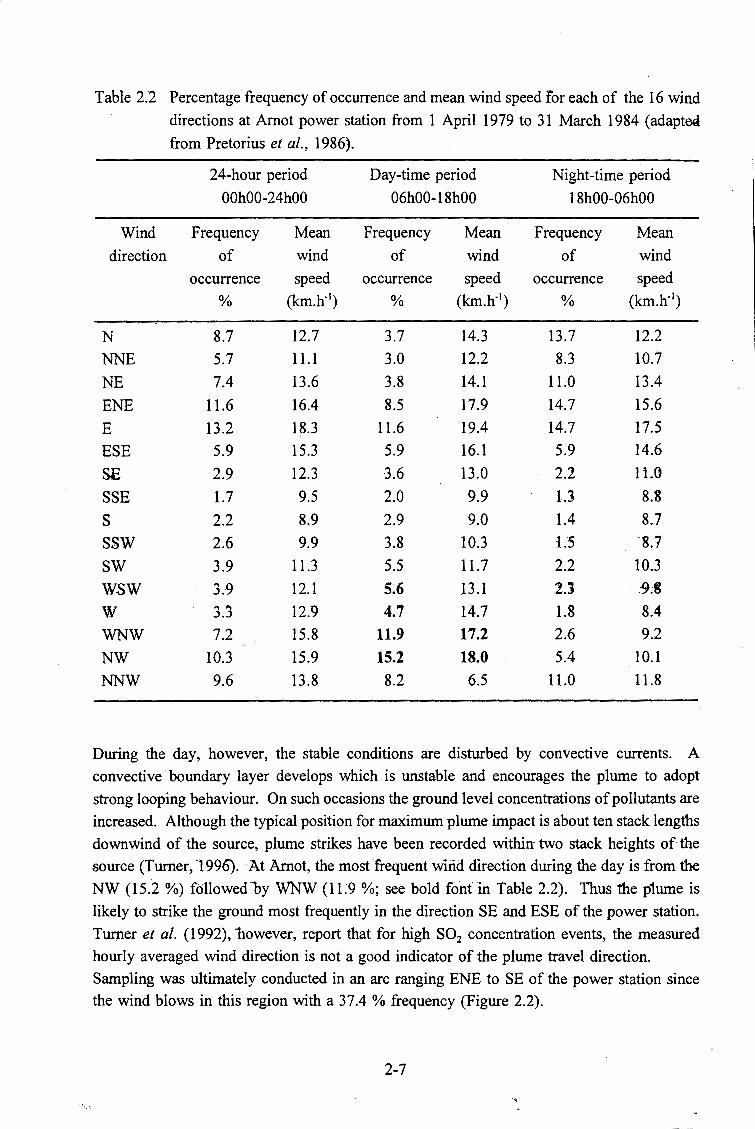
Table 2.2 Percentage frequency of occurrence and mean wind speed for each of the 16 wind

directions at Arnot power station from I April 1979 to 31 March 1984 (adapted

from Pretorius et al., 1986).

24-hour period Day-time period Night-time period

00h00-24h00 06h00- I 8h00 l 8h00-06h00

Wind Frequency Mean Frequency Mean Frequency Mean

direction of wind of wind of wind

occurrence speed occurrence speed occurrence speed

% (km.h"1) % (km.h"1

) % (km.h"1)

N 8.7 12.7 3.7 14.3 13.7 12.2

NNE 5.7 11.1 3.0 12.2 8.3 10.7

NE 7.4 13.6 3.8 14.l 11.0 13.4

ENE 11.6 16.4 8.5 17.9 14.7 15.6

E 13.2 18.3 11.6 19.4 14.7 17.5

ESE 5.9 15.3 5.9 16.l 5.9 14.6

SE 2.9 12.3 3.6 13.0 2.2 l l.{}

SSE 1.7 9.5 2.0 9.9 LJ 8.8 s 2.2 8.9 2.9 9.0 1.4 8.7

SSW 2.6 9.9 3.8 10.3 l.S ·g.7

SW 3.9 11.3 5.5 11.7 2.2 10.3

WSW 3.9 12.l 5~6 13.l 2.3 -9;8

w 3.3 12.9 4.7 14.7 1.8 8.4

WNW 7.2 15.8 11.9 17.2 2.6 9.2

NW 10.3 15.9 15.2 18.0 5.4 IO.I

NNW 9.6 13.8 8.2 6.5 11.0 11.8

During the day, however, the stable conditions are disturbed by convective currents. A convective boundary layer develops which is unstable and encourages the plume to adopt

strong looping behaviour. On such occasions the ground level concentrations of pollutants are

increased. Although the typical position for maximum plume impact is about ten stack lengths

downwind of the source, plume strikes have been recorded within- two stack heights of the

source (Turner, -1996). ·At Arnot, the most frequent wiiid direction during the day is from the NW (15.2 %) followed by WNW (I L9 %; see bold fonfin Table 2.2). Thus the p1ume is

likely to strike the ground most frequently in the direction SE and ESE of the power station.

Turner et al. (1992), bowever, report that for high S02 concentration events, the measured

hourly averaged wind direction is not a good indicator of the plume travel direction.

Sampling was ultimately conducted in an arc ranging ENE to SE of the power station since

the wind blows in this region with a 37.4 % frequency (Figure 2.2).

2-7

.. ··

·········· Power lines - ·Drainage - Roads - - Access roads - Railway line •Pans ~ Arnot town

N

i

0 1 2 3 4 .· S km

Figure 2.2 Location of soil sampling sites in relation to Arnot power station.

A detailed study of S02 dispersion at Matimba power station showed the importance of wind

speed in determining plume behaviour (Turner et al., 1992). Episodes of high S02

concentrations at ground level and closest to the source were generally experienced during

very light wind conditions (less than 3.6 km.h·1 at 96 m above ground level). The data

presented in Table 2.2 show that for the selected WSW to NW wind directions, the mean wind·

speeds ar~ high (between 13 and 18 km.h·1 at 10 m above ground level). Wind speed

generally increases with altitude, so the pre-condition of light winds for maximum looping

close to the source would .~ot apply in the selected wind directions. Presumably ground

contact of the plume under high wind speed conditions would simply be further from the

source than the 2.5 km touch down point reported by Turner et al. (1992).

2.3.3 Land use

Coal mining and agriculture are the main land uses in the region. Maize cultivation, and to

a limited extent, livestock farming, are the major agricultural activities. Sampling sites were

restricted to natural grassland showing minimal evidence of recent, intensive grazing by livestock, wherever possible (Figure 2.3).

2-8

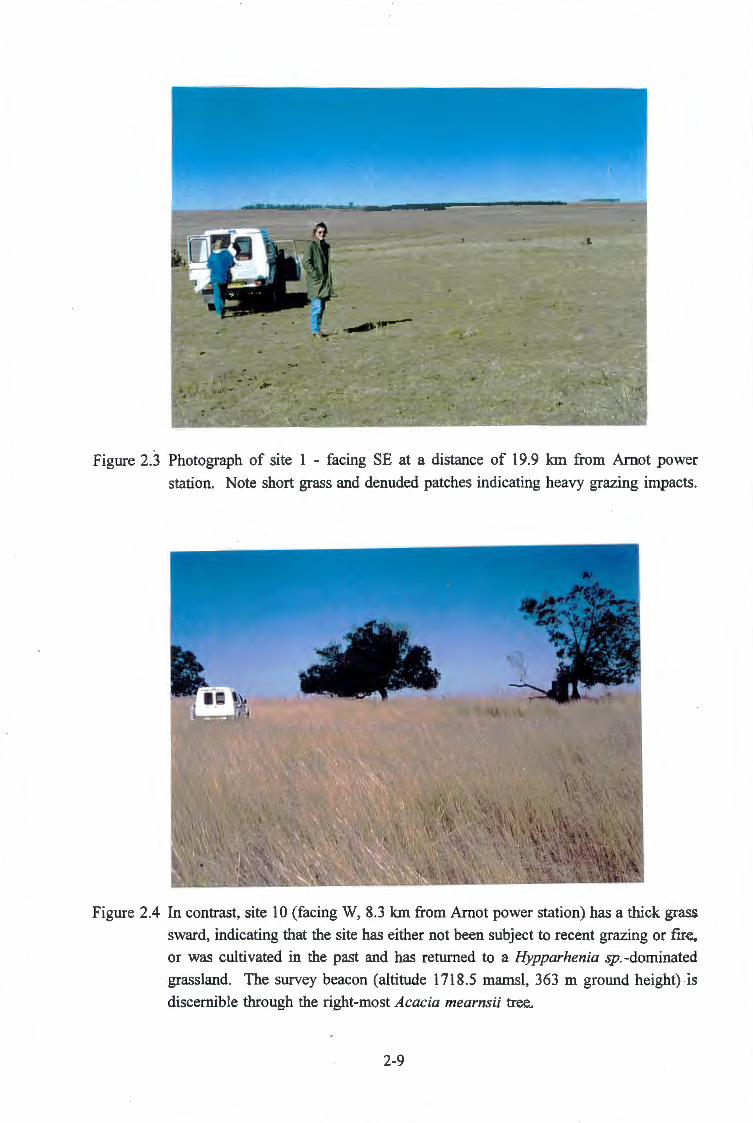
Figure 2.3 Photograph of site 1 - facing SE at a distance of 19.9 km from Arn-ot power

station. Note short grass and denuded patches indicating heavy grazing impacts.

Figure 2.4 In contrast, site 10 (facing W, 8.3 km from Arnot power station) has a thick grass

sward, indicating that the site has either not been subject to recent grazing or fire_,

or was cultivated in the past and has returned to a Hypparhenia sp. -dominated

grassland. The survey beacon (altitude 1718.5 mamsl, 363 m ground height) is

discernible through the right-most Acacia mearnsii tree~

2-9

2.3.4 Land Type and topography

Much of the South African landscape has been classified into terrain units which serve as

indicators of agricultural potential. The terrain units are delineated on the basis of uniformity

of terrain form, pedosystems and finally climate zones. The area surrounding the Arnot power

station is primarily occupied by a plinthic catena (Land Type Memoirs 2528 Pretoria, 1987)

which is further separated into two terrain units, Ba and Bb, on the basis of a

pedological/terrain form boundary. The unit Ba indicates land in which red and/or yellow

apedal soils (Hutton, Bainsvlei, A val on, Glencoe and Pinedene forms) that are dystrophic

and/or mesotrophic predominate over red and/or yellow soils that are eutrophic. Red soils

occupy more than a third of the area. The Bb land unit differs only in that the red soils are

not widespread. As a consequence of the similarity of the landtypes sampling sites could be

selected which fell on either Ba or Bb. For the record, sites 1, 6, 10, 11, 12, 13, and 15 fall

within land unit Ba while the remaining sites (sites 2, 3, 4, 5, 7, 8, 9 and 14) fall within land

unit Bb. Note that the soils described above follow the classification of MacVicar et al.

(1977). In all units the valley bottoms are occupied by gley soils such as the Rensburg form.

Site 10 is, however, an exception to the general description of the landscape as it was occupied

by a Rensburg soil of the Phoenix series (non-calcareous in the G-horizon) and was situated

on a hill crest (Figure 2.4).

The general topography of the area is characterised by gently rolling hills with a midslope

length ranging between 500 - 1 500m and a maximum slope of 15 % (Land Type Memoirs

2528 Pretoria, 1987). The undulating nature of the landscape is evident in Figure 2.5.

Roberts and Bettany (1985 - cited in Fey et al., 1996) showed that topography influenced the

form and amount of sulphur within a soil profile. · Soils in the lower landscape had more

soluble sulphate and organic sulphur, and greater sulphate accumulation at depth, than soils

in higher positions on a slope. The accumulation of sulphate in bottomlands due to processes

of illuviation down a slope would confound interpretations with respect to sulphate of

atmospheric origin. Thus sampling was restricted to the upper- and midslopes; bottomlands

were not sampled at all.

The higher portions of the landscape are also more likely to intercept pollution plumes than

the valley bottoms. Annegarn et al. ( 1996) found a greater concentration of sulphur dioxide

at a monitoring site that was elevated 150 m above the surrounding terrain. Thus sampling

of the upper slopes increases the likelihood of intercepting plume touchdown.

2-10

Figure 2.5 Site 7 viewed when facing W towards Arnot power station (8.1 km distant). The

pollution plume is evident as is the gentle topography of the landscape.

2.3.5 Accessibility

Ease of access to the sampling sites was an additional criterion for selection although not an

overriding one. Wherever possible, sites were selected on either Eskom or Amcoal property

as land use on these properties are unlikely to change in the foreseeable future. Eskom is the

major electricity generator in South Africa, while Amcoal is the mining division of Anglo­

American which supplies coal to Eskom. When sites were located on private land, permission

from the landowner was always sought.

2.3.6 Geology

Although parent material is a primary determinant of the nature of soil, geological features

were not used as criteria, especially since the geology is fairly uniform. The sampling area

is primarily underlain by interbedded shale, shaly sanstone, sandstone, grit and conglomerates

of the Ecca formation, and interbedded tillite and shale of the Dwyka formation; both

formations are of the Karoo sequence. These sedimentary rocks are intruded by coarse-grained

dolerite. Some outcrops of Steenkampsberg quartzite and sub-ordinate shale of the Pretoria

group are located in the easterly portion of the sampling area (Department of Mines, 1978;

2528 Pretoria 1 :250 000 Geological Series map, Government Printer, Pretoria). Specific information with respect to rock type is provided for each sampling site (Appendix l).

2-11

2.4 Sample collection and preparation

Having identified the area south-east and east-south-east of the power station as the most

appropriate for sampling, specific sites were selected using a combination of orthophotographs,

a 1 :50 000 topocadastral map (Chief Directorate: Surveys and Land Information 2529DD

Arnot, 1986) and a preliminary reconnaissance. The location of sampling sites is shown in

Figure 2.2. Sampling was conducted from 5 to 9 August 1996.

Once a sampling site was selected using the criteria outlined in section 2.3, a centrepoint was

selected at random. Care was taken to ensure that the entire sampling area was clear of

features such as roads, tracks, kraal sites, stock feeding sites or rock ridges. Smaller features

such as animal burrows and termite mounds could not be avoided but we ensured that soil

samples were not taken near these. Notes were made of site features such as approximate

distance to fences, windpumps, trees, farmgates and other landmarks. Each site is described

in this manner in Appendix 1.

Since the establishment of baseline monitoring sites is an objective of this study, the exact

location of each site must be known so that the correct sites can be resampled in the future.

A GARMIN GPS 45 navigator was used to locate the position of the centrepoint of each

sampling site. The Geographical Positioning System (GPS) is operated by the government of

the United States of America, which is solely responsible for its accuracy and maintenance.

The system is currently under development and is subject to changes which could affect the

accuracy and performance of all GPS equipment. Thus, supplementary information from local

maps and describing site-specific features was essential to ensure that each site could be

relocated in the future.

The GARMIN GPS 45 features a MultiTrac8™ receiver which tracks and uses up to eight

satellites simultaneously. Position accuracy ranges from 5 to 15 meters. The map datum field

used as the default setting is the World Geodetic System 1984 (GARMIN GPS 45 Instruction

Manual) .

The centrepoint can be considered the hub of a wheel with a radius of 25 m (Figure 2.6). A

soil sample was taken at the end of each of eight spokes which were roughly equal distances

apart. Two additional samples were taken on opposite spokes 12 m from the centre - to give

a total of 10 samples which were combined to give one composite sample for each site. The

area sampled thus covered an area of about 1 970 m2•

2-12

•

25m 25m

• = subsample collection point

Figure 2.6 Sampling wheel showing the relative positions of samples to each other. Samples

were combined to form one composite sample for each site.

At each point a topsoil and subsoil sample were taken. Topsoil was collected as follows: The

soil surface was scraped clean of vegetation and loose material with a spade. A square of

spade width (250 mm) was chopped into the soil surface to a depth of 10 cm. Once lifted,

the soil clod was then quartered and taken to the centrepoint where it was deposited on a thick

plastic sheet. Once all ten topsoil samples were collected, the clods on the plastic sheet were

broken down, large roots and stones discarded and the soil well mixed to give a single

composite sample. A two liter plastic screw-top bottle was filled with soil, as was a large;

clear plastic bag. Both bottle and bag were labelled and sealed with masking tape.

Approximately 4 kg soil was taken for each sample. Subsoil was sampled by augering deeper

into the existing hole, until the auger tip was at a depth of 20 cm. Any soil in the auger

blades was discarded. Further augering, to a depth of 40 cm, resulted in a sub-soil sample

from 20 - 40 cm in the soil profile. As with the topsoil sample, the subsoil was broken down,

mixed, bagged and labelled as a composite sample for that site.

Each site was sampled only once in this manner. Time and labour constraints did not allow more samples to be taken and this limitation must be considered during data interpretation.

Sampling the top- and subsoil samples will give an indication of the geochemical feasibility

of establishing long-term monitoring sites in the vicinity of Arnot. Based on the preliminary

findings, the sites could be revisited to allow the description and classification of soil profiles

for each site.

2-13

2.5 Validation of samp)ing protocol

The information gathered in this exercise is intended to provide the baseline data with which

future work can be compared. However, within-site variability can be quite high, and some

indication of the variability inherent at a site is thus necessary.

An attempt to validate the ~ampling protocol was made by revisiting thre~ sites and repeating

the sampling. Ideally, someone without any previous knowledge of the site should have

performed the resampling - using a GPS, the topographical map and site descriptions to

identify the sites. However, this was not feasible so I revisited three sites myself and tested

. the repeatability of sampling.

2.5.1 · Materials and methods

A different GPS navigator unit was used but of the same make (GARMIN 45 GPS). Since

I had prior knowledge of the site I could easily find the site and remembered the location of

the centrepoint of the sampling wheel and recorded the position given by the GPS without

knowing beforehand what they should be. The co-ordinates for both visits are presented in

Table 2.3. Soils were resampled according to the original protocol. The three sites were

revisited on 20 October 1996 and sampled in the same way. Time constraints limited sample

collection to the topsoil only.

Preliminary air-drying and sieving was done at the CSIR laboratories in Nelspruit. The

measurement of pH in water, KCl and K2S04, and EC, was performed in the Geology

Department at the University of Cape Town. Organic carbon by wet oxidation, ANC and

anions in saturated paste solutions were also determined. Details of eacp. method are given

in Appendix 2. Only a few analyses were performed in order to get an impression of

repeatability of the sampling.

2-14

2.5.2 Results and discussion

Finding the sites with the use of the maps and site descriptions was simple but the position

of the centrepoint was not as easy to find, even though I was familiar with the site. While

exploring the site, the original sampling holes could be found and were used as guides to

estimate the location of the centrepoint. At the centrepoint the GPS reading was recorded, and

can be compared with the original position (Table 2.3). The greatest discrepancy was recorded

for latitude at site 6 - a difference of 0.027' - which amounts to approximately 46 m.

However, the identification of this site was less certain than the other two sites sampled. The

smallest discrepancy was 2 m from the original centrepoint. The GPS has a recognised error

of 15 m, so the general repeatability of the GPS for the remaining sites is either within or

slightly over that error margin.

Subsamples were taken near to the original sampling holes and pooled to give a composite

sample. The results presented in Table 2.3 show that, to a large extent, the findings for the

different sampling times are quite similar. Despite the 46 m discrepancy in the latitudinal

position of the site 6 centrepoint, the values obtained for anions, pH, organic carbon and ANC

were very similar. However site 13 showed a.doubling in the concentration of Cl, N03, and

S04, which is also reflected in the higher value for electrical conductivity. The extracts were

repeated to ensure that analytical error was not the cause of the differences. The estimates of

percentage organic carbon also show some range in values. Obviously more replicates are

necessary for a statistically valid comparison and more sites should be included. By collecting

composite samples over a large area it was hoped that within-site variability would be

minimised.

Freedman and Hutchinson (1980) found with-in site variability to be high in their study of a

deposition gradient from a nickel-copper smelter in Sudbury. Six samples from a site had

been combined to form one composite sample for the Subury site whereas ten samples made

up the composite sample in the present study. A far more intensive sampling strategy was

employed by Stuanes et al. (1995) in a similar study were soils were sampled from 50 points

in a grid of 10 m by 20 m in size. Sampling was repeated four times for each grid.

Unfortunately the authors gave no information on within-site variability. These two examples

from the literature illustrate that sampling intensity should be given careful consideration. The

most efficient and effective sampling strategy will depend on the inherent variation of each

site.

2-15

Tab

le 2

.3

Com

pari

son

of

sele

cted

ana

lyti

cal

data

for

sam

ples

tak

en i

n A

ugus

t an

d O

ctob

er f

or t

hree

sit

es.

Sit

e 6

Sit

e 13

S

ite

15

Aug

ust

Oct

ober

A

ugus

t O

ctob

er

Aug

ust

Oct

ober

Pos

itio

n co

-ord

inat

es

25°5

6. l

42'S

25

°56.

l 69

'S

25°5

8.74

0'S

25

°58.

749

'S

25°5

7.34

5'S

25

°57.

342'

S

29°4

7.89

2'E

29

°47.

909'

E

29°4

9.94

8'E

29

°49.

947'

E

29°4

7.08

7'E

29

°47.

077'

E

Ani

ons

in s

atur

ated

pas

te

solu

tion

(m

g.L

-1 )

Cl

23.3

27

.3

8.5

18.1

24

.3

27.3

N

03

1.9

1.3

0 1.

0 0.

5 1.

2 S

04

40.6

43

.0

19.8

42

.8

48.6

51

.2

EC

(µS

.cm

-1 ) 29

1 24

5 14

4 21

0 27

3 28

8 (n

=2)

(n

=2)

p

H (

wat

er)

5.2

5.2

5.8

5.7

5.9

5.9

pH

(K

Cl)

4.

1 4.

1 4.

4 4.

4 4.

5 4.

6 pH

(K

2S0

4) 4.

6 4.

6 4.

8 4.

8 4.

9 5.

0

Org

anic

car

bon

(%)

2.3

2.2

1.8

2.1

2.2

2.8

AN

C (

cmol

c.L

-1 ) 2.

5 2.

6 2.

9 2.

9 3.

7 4.

1

2-16

Ideally, the validation of a sampling protocol should be far more comprehensive than the

approach adopted in this study. Ramsey et al. (1995) have shown that the principles of the

collaborative trial, where the performance of an analytical method is assessed, can be applied

to sampling strategies. In a collaborative trial a number of workers would independently

follow the sampling instructions for a particular site; the collected samples would then be

analysed µrider repeatable conditions (i.e. in a single run in one laboratory) to avoid

confounding analytical variations with sampling variations. Such an exercise allows estimates

to be made of the uncertainties associated with the sampling method. The suitability of the

sampling protocol can then be evaluated.

Seasonal variation can be an important confounding factor in studies which require resampling.

Tabatabai (1982) states that the sulphur status of soil will vary on a seasonal basis. The

sampling period for this study extended over the dry winter months when sulphate:movement

in rainwater leachate is minimal. To achieve reproducibility, resampling for long-term

monitoring purposes should be done in the dry season.

2.5.3 Conclusions

The sampling procedure described above represents a preliminary stage in the establishment

of long-term monitoring sites near a power station. The repeatability of the sampling protocol

appears to be satisfactory. The method of testing was, however, based on a superficial

examination of the results obtained for a few analytical procedures. The reproducibility of the

sampling protocol, in which several workers independently sample the site in a predetermined

fashion, should be tested by the application of a collaborative trial approach, as advocated by

Ramsey et al. (1995). A more rigorous assessment of the sampling protocol is essential if the

data are to contribute to a long-term monitoring programme.

In addition, the number of sites to be sampled at some future time ma_y be reduced if

geochemical evidence indicates unusual sites which warrant exclusion from the data set. The

provision of acclirate geographical information and site descriptions enables each site to be

revisited for more detailed description and classification of soil profiles ~t any time in the

future.

2-17

CHAPTER3

DETERMINATION OF SOIL SULPHATE

3.1 Introduction

Sulphur is a key element operating in biogeochemical cycles and exists in a variety of forms

and oxidation states. In terms of global reservoirs, most of the sulphur at any time is found

in the lithosphere. The weathering of sulphide-bearing minerals in rocks releases sulphur as

sulphate. Since sulphur is a necessary nutrient for all forms of life, much of the sulphate is

incorporated into the biomass through plant uptake and microbially mediated reactions. The

organically bound sulphur is then released back to the soil through decay and mineralisation

reactions (Freney and Williams, 1983; Charlson et al., 1992). Under certain climatic

conditions, the decay processes may be arrested and the subsequent accumulation of organic

matter be converted to coal, peat or petroleum gas. The anthropogenic combustion of these

fossil fuels accelerates the transfer of sulphur between the lithosphere and the atmosphere.

Sulphur in soils can be broadly grouped into organic sulphur, accounting for over 95 % of the

total sulphur in soils, and inorganic sulphur. The inorganic fraction is dominated by sulphate

in oxidising environments and occurs as water soluble salts, in insoluble forms or as sulphate

adsorbed onto soil colloids (Tabatabai, 1982). The term labile sulphate refers to both the

water-soluble and sorbed fractions.

The accurate determination of soil sulphate is an essential requirement in evaluating whether

or not anthropogenic impacts from the oxidation of fossil fuels are occurring. A long-term

monitoring system established to detect impacts requires reliable baseline data and a consistent

method of analysis in order to make valid comparisons between present and anticipated

conditions. In the following chapter, two methods for the chemical analysis of labile sulphate

are compared and the suitability of each method to meet these requirements is assessed.

3.2 Methods of sulphur determination

Much of the sulphur in soil is bound in the organic fraction which is normally estimated from

the difference between total sulphur values and the inorganic sulphate values (Tabatabai,

1982). Total S is usually determined by the conversion of the various sulphur forms by

oxidation to one form - such as sulphate - which is then determined by colorimetry, gravimetry, turbidimetry or by ion exchange. Total S can also be accurately determined by x-ray fluorescence spectroscopy (XRFS) (Tabatabai, 1982).

3-1

Sulphate is the most common form of inorganic sulphur in soils, particularly in well-drained

and well-aerated soils. Freney (1961, cited in Tabatabai, 1982) estimates the amount of

reduced sulphur compounds at < 1 % under such conditions. No attempts were therefore made

in the current study to convert reduced S-compounds to sulphate prior to determination. Since

sulphate can be sorbed onto soil surfaces, the amount that is measurable depends on the

fraction that is released by the soil surface. The capacity of a variety of solutions to extract

sulphate is reviewed by Tabatabai (1982). The water soluble sulphate fraction can be

extracted with water while various chloride and phosphate salts are suggested for extraction

of the adsorbed fraction. Fox et al. (1964, cited in Tabatabai, 1982) found 0.01 M

Ca(H2P04) 2.H20 to be most effective; the phosphate in the solution, in the concentration of

about 500 mg.L-1 P, is able to displace most of the adsorbed sulphate of many soils and the

resultant extract is easier to filter than an extractant such as KH2P04• The sulphate can then

be determined by colorimetry, turbidimetry, titrimetry, gravimetry or ion chromatography.

Tabatabai (1982) recommends the colorimetric method developed lJY Johnson and Nishita

(1952) as the most accurate means of determining sulphate. However, the method requires

specialised glassware and reagents and is labour intensive. Of the methods listed, turbidimetry

· and ion chromatography are discussed further since these were the two techniques exploited

in the present study.

Turbidimetric determination of extractable sulphate is a widely practised technique employed

by many laboratories, although a number of problems are associated with the method. In

principle, sulphate in solution reacts with an excess of barium chloride which forms insoluble

barium sulphate. The turbidity of the resultant solution is measured by the amount of light

attenuated through scattering by the precipitate, and is then determined spectrophotometrically.

High variability plagues turbidimetric determinations, and there can be considerable uncertainty

concerning the accuracy of the results (Adams et al., 1984 ). Variability can stem from

interference from other solutes or incomplete precipitation reactions. Despite these flaws,

turbidimetry is widely used because it is a simple and rapid means of analysing for sulphate

in aqueous solutions.

Ion chromatography is a relatively modem technique for the determination of sulphate

inorganic ions in aqueous solution. Ion chromatography (IC) separates ions in a sample on

the basis of differential affinity for an ion exchange surface. The sample is carried by a

mobile phase - the eluent - through an ion exchange resin which represents the stationary

phase. The dense packing of resin-beads in the exchange column requires that the eluent be

under high pressure in order to pass through the column. The ions progress through the

column at different rates and therefore enter the detector at different times. The ions are

detected by the increase in electrical conductivity of the mobile phase and are reported as

conductivity peaks on a chromatogram. The elution time is specific to a particular ion and

the peak area or peak height is proportional to concentration, which is determined after

appropriate calibration with standard solutions (Willard et al., 1988).

3-2

Ion chromatography is a method which has been extensively evaluated and can be regarded

as reliable as well as recommended for the determination of common ions such as sulphate.

It is well recognised as being a sensitive technique with detection limits, accuracy and

precision being instrument dependent (Fifield, 1995; Watson, 1994, Method No. W75, pg 537

& 617). Although recognized as having wide potential applications, to my knowledge, the

general literature reports no instances where IC has been used for the determination of

phosphate-extractable sulphate. The high concentration of phosphate in the extract would

generally require dilution in order to avoid overloading the anion exchange column and

sulphate is consequently anticipated to be diluted beyond detection. Thus the use of IC for the

determination of phosphate-extractable sulphate represents a novel application of the technique.

3.3 Materials and methods

3.3.1 Extraction of water-soluble sulphate

An aqueous extract of each soil was prepared from 500g of soil saturated to field capacity,

using the method of Rhoades (1982a), details of which are given in Appendix 2. The extract

was filtered through a 0.45 µm filter to remove colloids, followed by a Dionex On-Guard-P

cartridge for removal of organic compounds.

3.3.2 Extraction of the adsorbed sulphate fraction

The extraction of adsorbed sulphate was performed in the laboratories of the Grain Crops

Institute at Cedara, Pietermaritzburg, KwaZulu-Natal. Sulphate was extracted with 0.01 M

Ca(H2P04)i.H20 containing 10 mL Superfloc per litre. A 2.50 g sample of air-dry soil

( < 2 mm fraction) was weighed into soil cups, to which 25 mL of the calcium phosphate

solution was added by automatic dispenser. The solution was then stirred for 30 minutes on

an automated stirring apparatus. Solution and soil were filtered through approximately 2 g of

sulphur-free carbon held in Whatman No. 1 filter paper to remove any organic colouration

from the extract prior to turbidimetric analysis.

',3.3.3 Sulphate determination by turbidimetry

Turbidimetric analysis for sulphate was also performed m the Grains Crop Institute

laboratories at Cedara, using an auto-analyzer method. Solutions for the auto-analyzer were

prepared according to the directions given by Wall, Gerhrke and Suzuki ( 1986). Calibration

standards of 0, 5, 10, 15 and 20 ppm S were prepared in the soil extracting solution. A batch

of 43 samples could be analyzed at a·-time, but these included calibration standards, distilled

3-3

water blanks, extractant blanks and a control soil of known sulphate concentration.

Determinations of the control soil and the calcium phosphate extraction blank were each

repeated three times during each analytical run and the 10 ppm S calibration standard was

repeated twice. The concentration of sulphate was determined from a calibration curve, after

which the extractant blank value was subtracted from the sample value.

Five extractions and analytical runs were performed, giving at least three determinations of

extractable sulphate for each sample; in some cases four were obtained. Two samples of

saturated paste extracts were also analyzed but the small solution volume permitted only one

determination of the water-soluble sulphate.

3.3.4 Sulphate determination by ion chromatography

Each sample was diluted appropriately to achieve an electrical conductivity less than

100 µS.cm- 1 in order to avoid over-loading the exchange column. For the saturated paste

extracts the dilution factor was either two or five, whereas the calcium phosphate extracts

required a tenfold dilution. All samples were filtered prior to analysis as described in

section 3.3.l.

A DIONEX 300 ion chromatography system and associated software was used for the

determination of sulphate. The determination was performed on a Dionex HPIC-AS4A-SC

anion exchange column with carbonate/bicarbonate eluent and conductivity detection, using

peak area as the basis for determination. The run conditions were as follows:

Sample loop volume: 50 µL

Guard column: Dionex HPIC-IonPac AG4A

Separator column: Dionex HPIC-IonPac AS4A-SC

Eluent: l.80mM N~C03 and 1.70 mM NaHC03

. Eluent flow rate: 2.0 mL.minute-1

3.4 Results and discussion

The concentrations of sulphate in saturated paste extracts are presented in Table 3.1. Where

possible a repeat determination was performed, but samples and replicates are insufficient to allow a full statistical comparison. Analyses performed on the same day were highly

repeatable (samples indicated by n=2 or n=3).

Table 3. I shows the similar concentrations of sulphate obtained by both IC and turbidimetry

for the two saturated paste extracts (ST and 7T).

3-4

Table 3.1 Concentrations of water soluble sulphate in saturated paste extracts determined by

ion chromatography and turbidimetry (mg SO/.L·1). Topsoils are designated by -

T and subsoils by -S.

Ion chromatography Turbidimetry Sample

Assay on Assay on Mean s' 9/911996 27/9/1996

IT 32. l {n=3, s=0.07)

2T 22.7

3T 3S.O

4T 24.2 28.2 ST 33.8 29.7 31.8 2.9 30.3 6T 40.6

7T 34.2 29.5 31.9 3.3 34.0 ST 41.9 38.3 9T 41.5

IOT 2S.O

l lT 62.0

l2T 46.2 {n=2, s=0.02)

l3T 19.9

l4T 19. l

l5T 48.6

IS 18.4 17.S 2S 31.7

3S 2S.2

4S 18.9 (n=2, s=0.03)

SS 2S.2

6S 42.3

7S IS.5 {n=2, s=0.06)

8S 24.7

9S 17.4

IOS 41.l

l lS SI.7 12S 38.9 34.8 13S 20.3 14S 17.0 lS.2 ISS 21.6 {n=2, s=0.06)

1 s = one sample standard deviation

The results for the determination of extractable sulphate by turbidimetry are presented in

Table 3.2, together with the values obtained for the control soils and the extractant blanks.

The results of the turbidimetric determination are highly variable: for some soil samples the repeatability of analysis was good (eg 12T and 5S), whereas others displayed a wide range of

sulphate concentration (eg 3T, 7T and 2S). Sample means and standard deviations are presented in Table 3.2.

3-5

Tab

le 3

.2

Pho

spha

te e

xtra

ctab

le s

ulph

ate

dete

rmin

ed b

y tu

rbid

imet

ry.

Eac

h an

alyt

ical

run

is i

ndiv

idua

lly

pres

ente

d to

dem

onst

rate

the

vari

abil

ity

of

cont

rol

soils

and

bla

nks

betw

een

diff

eren

t ru

ns.

Top

soil

s ar

e de

sign

ated

by

-T a

nd s

ubso

ils

by -

S.

Sam

ple

Pho

spha

te e

xtra

ctab

le s

ulph

ate

(mg

sulp

hate

. kg

soi

l-1 )

Mea

n·

Sta

ndar

d R

elat

ive

devi

atio

n st

anda

rd

4/10

/199

6 I0

/9/1

996a

10

/9/1

996b

I0

/9/1

996c

9/

9/19

96

devi

atio

n (x

) (s

) %

IT

2U

16

.9

21.3

19

.7

2.5

12.6

2T

22

.0

2.2

15.9

13

.4

JO.I

75.7

JT

23

.6

2.S

9.1

11.7

10

.S

92.2

4T

11

.7

20.S

19

.S

17.3

4.

9 2S

.4

ST

22.0

26

.4

26.6

26

.4

2S.4

2.

2 S.

S 6T

29

.0

2S.9

29

.S

34.3

30

.S

2.6

S.4

7T

19.2

9.

1 13

.3

13.9

S

.l

36.S

ST

31

.6

4S.2

4S

.3

JS.2

41

.6

S.2

19.6

9T

17

.6

25.S

2S

.7

IS.2

21

.S

4.S

20.7

JO

T 11

.9

11.2

11

.2

S.9

10.S

1.

3 12

.l

llT

19

.2

20.4

20

.S

20.1

o.s

3.

9 12

T

2S.3

26

.7

27.2

28

.7

27.7

1.

0 3.

S 13

T

14.6

20

.7

22.4

7.

S 16

.4

6.6

40.4

14

T

20.4

20

.3

IS.S

IS

.S

2.S

14.S

!S

T

20.S

23

.3

13.0

IS

.9

S.3

2S.2

IS

0.

0 0.

0 0.

0 0.

0 0

2S

S0.7

19

.6

21.4

30

.6

17.4

S7

.0

JS

s.s

6.2

5.4

S.7

0.5

S.I

4S

21.6

21

.2

12.4

IS

.4

5.2

2S.2

SS

SO

.I 79

.2

so.s

S2.S

S0

.6

1.4

1.7

6S

66.0

60

.0

60.4

62

.0

62.l

2.

7 4.

4 7S

3.

4 4.

7 4:

7 S.

9 4.

7 1.

0 21

.9

SS

S9.6

60

.6

63.0

49

.4

SS.I

6.

0 10

.3

9S

0.0

0.0

0.0

0.0

0.0

0 !O

S 21

.S

23.2

26

.2

17.l

22

.0

3.S

17.3

!I

S

19.7

23

.4

23.5

23

.1

22.4

1.

8 S.

O

12S

0.0

0.6

4.S

0.0

1.3

2.1

169.

S IJ

S

2S.3

21

.9

22.0

IS

.2

21.1

4.

3 20

.2

14S

. 4S

.3

S2.3

4S

.S

4S.7

3.

5 7.

1 !S

S

70.2

63

.S

6S.t

67

.4

3.3

4.9

Con

trol

soi

ls

123.

4 12

6.7

124.

3 13

1 12

6.4

3.4

2.7

Ext

ract

ant

blan

ks

2.7

2.5

2.5

4.0

2.9

0.7

24.7

3-6

Samples 1 S and 9S repeatedly recorded zero values of extractable sulphate while sample 12S

recorded very low values of sulphate. Yet the absence of any extractable sulphate in samples

IS and 9S seems unlikely since both were found to have water-soluble sulphate, albeit in low

concentrations (Table 3.1). The explanation for this anomaly may lie in the subtraction of

the calcium phosphate blank, particularly for samples where the initial extractable sulphate

concentration is low. Fox et al. (1987 - cited in du Toit, 1993b) suggest that small amounts

of calcium phosphate can interfere with the precipitation of barium sulphate. Sulphate can be

underestimated in some soils because unknown constituents of the soil solution prevent the

precipitation of the barium sulphate. Fox et al. (1987) name soluble silica as one possible

culprit. The co-precipitation of barium phosphate may also be problematic, especially at low

sulphate concentrations when barium sulphate is minimal compared with barium phosphate (du

Toit, 1993b). These observations are supported by the more consistent results obtained for

the control soil, which has considerably more sulphate than any of the soils sampled.

Another explanation may be offered for soils with a large sorbing capacity for phosphate. If

phosphate is sorbed onto the soil surface in large amounts, the initial high phosphate

concentration that was accounted for in the blank may no longer be applicable to the sample.

By subtracting the calcium phosphate blank in these soils, an overcorrection would be effected,

resulting in negative values for sulphate. That interference from the calcium phosphate

extractant may occur is further ·substantiated by comparison of the water-soluble sulphate

concentrations which were determined by both IC and turbidimetry (samples 5T and 7T in

Table 3.1). In this case the extractant used was distilled water and the results for both

determinations are quite similar.

The soil extracts prepared on 4 October 1996 were used for direct comparison with ion

chromatography. To the author's knowledge, the use of ion chromatography to determine

phosphate-extractable sulphate has not been reported in the scientific literature. After

extraction and determination of the ·labile sulphate fraction at Cedara, the remaining solution

was couriered to the University of Cape Town for determination by IC. The values obtained

by IC were considerably higher than those obtained by turbidimetry (Table 3.3). To account

for the discrepancies the IC chromatograms were scrutinised more closely. Inspection of the

chromatograms revealed that, despite the apparent separation of peaks, there was still a degree

of overlap between the phosphate and sulphate peaks. The IC data were then reprocessed to

allow more accurate calculation of the area under the sulphate curve (Figure 3.1). At low

concentrations of sulphate the adjustment could reduce the .measured concentration by as much

as 7 %. Once dilution factors (IOx) had been accounted for and the concentrations had been

related to the soil mass (soil:extractant ratio = 1:10), the absolute error was magnified a

hundredfold. The original and processed IC data are presented in Table 3.3 along with the

results for turbidimetry.

3-7

Table 3.3 Concentration of extractable sulphate (mg SO/.kg·1 soil) in the soil collection

determined by turbidimetry and ion chromatography (IC). Topsoils are designated by -T and subsoils by -S.

Sample Turbidimetry IC -·uncorrected* IC - corrected*

IT 21.1 63.4 59.l 2T 21.6 82.6 77.4

·3T 23.l 74.1 68.6 4T 12.1 67.9 63.2 ST 22.2 95.8 91.l 6T 28.3 89.8 84.6 7T 18.8 103.3 97.2 8T 31.0 95.4 90.1 9T 17.4 84.5 79.3 lOT 12.0 57.7 53.4 I IT 19.0 87.5 81.9 12T 28.0 90.6 85.5 13T 14.2 52.9 48.6 14T 19.9 61.7 57.2 15T 20.0 58.8 54.0 IS 0.0 89.8 85.5 28 49.7 113.6 106.8 38 5.3 56.2 52.3 48 22.0 96.l 91.6 58 79.6 142.7 138.2 68 64.4 146.5 140.8 78 3.3 73.6 68.8 88 58.l 146.6 140.l 98 0.0 85.3 81.4 108 21.8 88.5 83.8 118 19.2 87.9 82.6 128 0.0 85.6 80.9 138 24.6 72.9 68.0 148 47.l 104.5 99.7 158 68.4 "121.7 116.2

* Correction involved accounting for the tailing of the phosphate peak under the sulphate peak as is shown in Figure 3.lb.

3-8

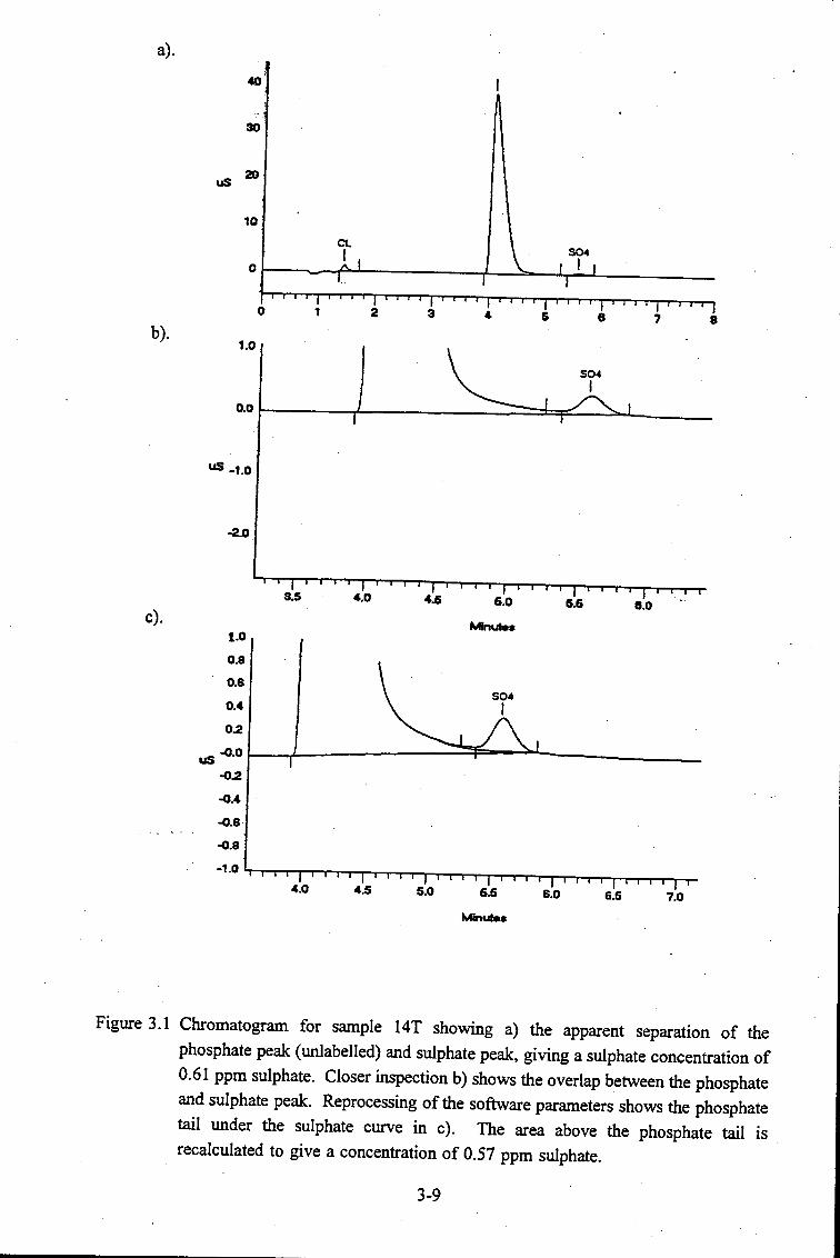
a).

40

30

uS 20

10

CL S0-4 I I 0

0 1 2 3 4 6 8 7 8 b).

1.0

us -1.0

-2..0

3.5 4.0 4.5 6.0 6.6 8.0 ...

c). Minutes

t.O

0.8

0.6 S0-4

0.4 I 0.2

us -0.0

-0.2

-0.4

-0.6

-0.8

-1.0

4.0 4.5 5.0 6.5 6.0 6.5 7.0

M"inutes

Figure 3.1 Chromatogram for sample 14T showing a) the apparent separation of the

phosphate peak (unlabelled) and sulphate peak, giving a sulphate concentration of

0.61 ppm sulphate. Closer inspection b) shows the overlap between the phosphate

and sulphate peak. Reprocessing of the software parameters shows the phosphate

tail under the sulphate curve in c). The area above the phosphate tail is recalculated to give a concentration of 0.57 ppm sulphate.

3-9

Phosphate-extractable sulphate values from Table 3.3 are plotted against the total sulphur

determined by XRFS in Figure 3 .2. The discrepancy in the values of extractable sulphate determined by IC and turbidimetry is readily apparent.

160

2140 A A x Turbidimeny 0

A IC - corrected ell

00 120 A ~

A 5100 A A

Cl.) A A -~ L::. A L::. A t::,A A ..c:: 80 A x A Q.. A -::s L::. t::.X x ell

L::. Cl.) 60 ~ L::. A - ~ .A .rJ x x ~ - 40 0

~ xX x >< 20 x. x ~xx x ~ x ~ x

x x x x x 0 "'

100 200 300 400 500 600 Total sulphur (mg S/kg soil)

Figure 3.2 Extractable sulphate determined by turbidimetry and IC plotted against total sulphur determined by XRFS.

A significant correlation was fotind between the results obtained by turbidimetry and IC

(r = 0.64, 28 d.f.) (Figure 3.3). Interestingly, the slope of the regression relationship between

the two methods is very close to one, suggesting that the overall difference between the two

is relatively constant, although the weakness of the regression also indicates that there is considerable random variation in this difference among the soils.

3-10

160

--co ~ 140

Q,) ..... = .g_ 120 :;

ti)

co 100 E '-" >. 80 ..c= c.. = -co 60 0 ..... x xx = s 40 0

..a (,)

c: 20 0 -

0 0 20 40 60 80

Turbidimetry (mg sulphate/kg)

Figure 3.3 The relationship between the extractable sulphate determined by IC and

turbidimetry (y=0.98x+59, r=0.64, 28 degrees of freedom); the equivalence line

(y=x) is plotted for comparison.

Wall et al. (1986) found the precision of the automated turbidimetric method to be excellent, reporting a relative standard deviation of 2.28 % for three independent analyses done in

duplicate on six soil samples. On the other hand, Adams et al. (1984) found turbidimetry to

be the least reliable of four methods used for the determination of soil sulphate. Turbidimetry

overestimated the sulphate added as a spike and generally gave higher values of sulphate

compared with other methods. Although based on the same principle of BaS04 precipitation,

the findings of Adams et al. (1984) are not directly comparable to the present study. Adams

et al. (1984) used the standard method for sulphate determination recommended by The

American Public Health Association (1971) and there are considerable differences in the

composition of the buffer solutions and experimental procedure compared with the method .. used in the ·laboratories at Cedara.

3-11

The present results show a large degree of variability and an apparent underestimation of

extractable sulphate by turbidimetry, possibly attributable to incomplete precipitation reactions.

Poor sulphate determination could also be caused by removal of more sulphate from standards

than samples by the decolorising charcoal, contamination of the charcoal by sulphate or

incomplete removal of colloidal particles by filtration (MC du Toit, 1993; Adams et al., 1984).

Despite its simplicity and ease of use, the automated turbidimetric method for sulphate

determination does not appear to be suited to the accurate determination of sulphate, particularly at low concentrations.

The high phosphate concentration (500 mg.L·1 P) of the extractant solution limits the

sensitivity of IC for the determination of sulphate since the soil extract must be diluted to

avoid overloading the exchange column. The sulphate present in the extractant solution is

consequently diluted to low concentrations (as low as 0.5 mg.L·1 sulphate), nearing the lower

limits of reliable detection for the sulphate anion (about 0.2 mg.L·1; JP Willis, personal communication).

Clearly, neither method is without its drawbacks. The strength of the extracting solution could

be reduced so that less dilution is required for IC. A concentration of approximately

200 mg.L·' P might prove strong enough to displace sulphate from soil surfaces and would

require less dilution, effectively increasing 2.5-fold the sensitivity of the IC method for

phosphate-extractable sulphate detection. A longer extraction time might also be effective.

In addition, a slower elution rate could be used so that anion peaks are narrower and more

easily measured off the chromatogram. The determination of extractable sulphate could be

done quite reliably provided there is careful processing of the IC data to eliminate peak

overlap. An added advantage of IC is that anions such as chloride, nitrite and nitrate can be determined simultaneously '." taking only eight minutes per sample to do so.

The data presented above suggest that the determination of extractable sulphate by turbidimetry

is inaccurate at low concentrations, confirming the findings of MC du Toit (1993), whereas

IC is generally acknowledged to be a reliable technique. Since water extractable sulphate was

measured in all samples by IC, the zero values obtained by turbidimetry for phosphate­

extractable sulphate show turbidimetry to be inappropriate for determinations of this nature.

Turbidimetry may be satisfactory to establish relative quantities of soil sulphate but remains suspect in terms of its accuracy.

3-12

3.5 Conclusions

Comparison of phosphate-extractable sulphate values showed those determined by turbidimetry

to be consistently below those determined by IC. The phosphate extractant solution appears

to be primarily responsible for the high variability and inaccuracies associated with the

turbidimetric determination, especially at low concentrations of sulphate. The subtraction of

the extractant blank may result in an over-correction for soils with a high phosphate-sorbing

capacity. Thus turbidimetry is not only inaccurate at low concentrations of sulphate but also

inconsistent as soils differ in their capacity to retain phosphate. Further work with

turbidimetry should focus on experimenting with soils of various phosphate sorption capacities

to establ.ish the subsequent effect on the accuracy of sulphate determination.

The use of ion chromatography for the determination of phosphate-extractable sulphate has not

been reported in the literature. Nevertheless, the preliminary results presented here suggest

that IC is potentially a viable, and probably more accurate method compared to turbidimetry,

for phosphate-extractable sulphate determination. Further evaluation of this new application

of ion chromatography is recommended, especially with relation to possible modification of

the extraction conditions and instrumental op~~ation to improve both sensitivity and accuracy.

3-13

CHAPTER 4.

PROPERTIES OF SOILS IN THE VICINITY OF ARNOT POWER STATION

WITH SPECIAL REFERENCE TO POTENTIAL AIR POLLUTION IMPACTS

4.1. Introduction

The monitoring of long-term changes has been identified by Wolters and Schaefer (1994) as

the best and most direct way of quantifying the effects of atmospheric deposition. During the

establishment oflong-term monitoring sites, the collection and characterization of the baseline

data is of primary importance and should be performed according to a range of standard

physical, chemical and mineralogical methods. Special emphasis should be placed on those

soil properties most likely to be impacted by atmospheric pollution - such as· parameters

related to soil acidity and soil sulphur status. Finally, wherever possible, relationships

between various soil properties should be identified as these may provide a firmer basis for

future comparison and possibly allow a comparison with sites elsewhere.

In this chapter, the suite of soils collected in the vicinity of Arnot power station is described

and the relationships between a range of parameters are explored.

4.2. Materials and methods

Details of the methods employed are provided in Appendix 2 or are cited from general texts.

The pH in distilled water, KCl and K2S04 was determined for each soil, using a 1 :2.5

soil:solution ratio. Acid neutralizing capacity (ANC) was determined according to the method

of du Toit and Fey (1994) and du Toit (1993a). Extractable base cations (Mg and Ca) and

extractable acidity were determined in 1 M KCl (Thomas, 1982). Extractable bases were

determined by atomic absorption spectrometry, while extractable acidity was determined by

potentiometric titration. Effective cation exchange capacity was calculated as the sum of

extractable acid and base cations. Acid saturation was then derived as extractable acidity* 100/ECEC.

Organic carbon by the Walkley-Black wet oxidation method, and citrate-bicarbonate-dithionite

(CBD) extractable Fe, Mn and Al were determined according to the methods outliJ;ied by

Nelson and Sommers (1986), and Jackson et al. (1986), respectively.

4-1

Saturated paste extracts were prepared by wetting 500 g of soil to field capacity then

extracting the soil solution by suction (Rhoades, 1982). Concentrations of anions and cations

in the soil solution were determined by ion chromatography, as described in Chapter 3.

Although phosphate-extractable sulphate was determined turbidimetrically (Wall et al., 1986),

only those values of extractable sulphate determined by ion chromatography were used.

Chapter 3 outlines the rationale for this decision and presents a description of the method employed.

The major elements (Si, Ti, Al, Fe, Mn, Mg, Ca, Na, K, S and P, reported as oxides) were

determined for all soils by XRFS using Norrish fusion discs. Powder briquettes were prepared

for the determination of trace elements (Mo, Nb, Zr, Y, Sr, U, Rb, Th, Pb, Zn, Cu, Ni, Co,

Mn, Cr and V) by XRFS.

The mineralogical study on the sand, silt and clay fractions was performed by X-ray

diffractometry by the ISCW in Pretoria. Particle size analysis was performed by

sedimentation using the hydrometer method.

4.3. Results and discussion

4.3.1. General soil properties

Table 4.1 shows the solid phase properties that were measured for each of the sampled soils.

The majority of the soils are classed as sandy loams or loamy sands, although 5 subsoils fall

into the sandy clay textural class. The highest clay content (30%) was recorded for the subsoil on site 10.

The most widespread parent material is the Ecca group of shales and sandstones, with

intrusions of dolerite dykes and sills. The sandstone influence is reflected in the dominance

of quartz in the silt and sand fractions. Less than 10 % feldspar occurs in 60 % of the soils

sampled. With one exception (site 10), the clay fraction is dominated by the 1: 1 layer silicate,

kaolinite, followed by mica. The soils of site 10 have an almost equal ratio of smectite to

kaolinite - a reflection of the doleritic parent material found in this region of the highveld

(Billunann, 1986). Although the goethite fraction is reported in Table 4.1 it is regarded as an

overestimation, as comparison with the total Fe20 3 determined by XRFS will show.

The dominance of quartz in the sand and silt fractions, and kaolinite and mica in the clay

fractions, indicates a moderate stage of soil development - according to the Jackson and

Sherman sequence of soil development (1953, cited in McBride, 1994).

4-2

.~-

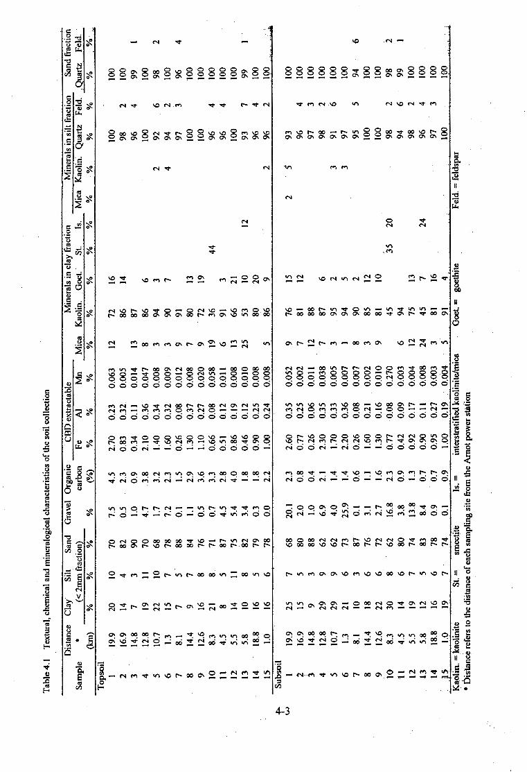
Tab

le 4

.1

Tex

tura

l, ch

emic

al a

nd m

iner

alog

ical

cha

ract

eris

tics

of t

he s

oil c

olle

ctio

n

Sam

ple

Top

soil

Dis

tanc

e

• (k

m)

1 19

.9

2 16

.9

3 14

.8

4 12

.8

5 I0

.7

6 1.

3 7

8.1

8 14

.4

9 12

.6

to

8.3

11

4.5

12

5.5

13

5.8

14

18.8

15

1.

0 S

ubso

il

l 19

.9

i 16

.9

3 14

.8

4 12

.8

5 10

.7

6 1.

3 7

8.1

8 14

.4

9 12

.6

10

8.3

11

4.5

12

5.5

.13

5.8

14

18

.8

l5

1.0

Cla

y S

ilt

San

d (<

2m

m f

ract

ion)

%

20

14

7 19

22

15

7 9 16

21

8 14

10

16

16

25

15

9 29

29

21

10

18

22

30

14

19

12

16

19

%

IO

4 3 ll

10

7 5 7 8 8 5 11

8 5 6 7 5 3 9 9 6 3 6 6 8 6 7 5 6 7

%

70

82

90

70

68

78

88

84

76

71

87

75

82

79

78

68

80

88

62

62

73

87

76

72

62

80

74

83

78

74

Gra

vel

Org

anic

C

BD

ext

ract

able

ca

rbon

-F

-e--A

l---M

n--

%

(%)

7.5

0.5

1.0

4.7

l.7

7.2

0.1 I.I

0.5

0.7

4.5

5.4

3.4

0.3

0.0

20.l

2.

0 1.

0 6.

9 4.

0 25

.9

0.1

3.1

2.7

16.8

3.

8 13

.8

8.4

0.9

0.1

4.5

2.3

0.9

3.8

3.2

2.3

1.5

2.9

3.6

3.3

2.8

4.0

1.8

1.8

2.2

2.3

0.8

0.4

2.1

1.4

1.4

0.6

l.l

1.6

2.3

0.9

1.3

0.7

0.7

0.9

%

%

%

2.70

0.

23

0.06

3 0.

83

0.32

0.

005

0.34

0.

11

0.01

4 2.

IO

0.36

0.

047

1.40

0.

34

0.00

8 1.

60

0.32

0.

009

0.26

0.

08

0.01

2 1.

30

0.37

0.

008

l.10

0.

27

0.02

0 0.

66

0.08

0.

058

0.51

0.

12

0.01

1 0.

86

0.19

0.

008

0.46

0.

12

0.01

0 0.

90

0.25

0.

008

1.00

0.

24

0.00

8

2.60

0.

35

0.77

0.

25

0.26

0.

06

2.30

0.

35

1.70

0.

33

2.20

0.

36

0.26

0.

08

1.60

0.

21

1.30

0.

16

0.77

0.

08

0.42

0.

09

0.92

0.

17

0.90

0.

11

0.95

0.

27

1.00

0.

19

0.05

2 0.

002

0.01

1 0.

038

0.00

5 0.

007

0.00

7 0.

002

0.01

0 0.

270

0.00

3 0.

004

0.00

8 0.

003

0.00

4

Min

eral

s in

cla

y fr

actio

n M

ica

Kao

lin.

. Goe

l.

St.

Is.

%

%

12

72

86

13

87

8 86

3

94

3 90

9

91

7 80

9

. 72

19

36

6 91

13

6

6

25

53

80

5 86

9 7 12

7 3 l 8 .3 9 6 12

24

3 5

76

81

88

87

95

94

90

85

81

45

94

15

45

81

91

%

16

14

6 3 7 13

19

3 21

IO

20

9 15

12

6 2 5 2 12

IO

13

7 16

4

%

%

44

12

35

20

24

Kao

lin.

= ka

olin

ite

St. =

sm

ecti

te

Is.

=

inte

rstr

atif

ied

kaol

init

e/m

ica

Goe

l. =

goe

thit

e •

Dis

tanc

e re

fers

to

the

dist

ance

of e

ach

sam

plin

g si

te f

rom

the

Arn

ot p

ower

sta

tion

Min

eral

s in

sil

t fr

actio

n S

and

frac

tion

M

ica

Kao

lin:

Qua

rtz

Feld

. ,Q

uart

z Fe

ld.

%

%

%

%

%

.%

2

2 4 2 3 3

Feld

. =

fel

dspa

r

100

98

96

100

92

94

97

100

100

96

96

IOO

93

96

96

93

96

97

98

91

97

95

100

100

98

94

98

96

97

100

100

2 10

0 4

99

100

6 98

2

100

3 96

10

0 10

0 4

100

4 10

0 10

0 7

99

4 10

0 2

190

4 3 2 6 5 2 6 2 4 3

100

100

IOO

IOO

100

100

94

100

100

98

99

100

100

100

100

2 4 6 2 l

. '··

---------------

Table 4.2 shows the major element composition while trace elements are shown in Table 43. Although the elemental composition, mineralogy and particle size of soils can generally be

related to parent material (McBride, 1994 ), the work of Buhmann ( 1986) on soils of the

highveld showed that dolerite and upper Ecca shale weather to soils with very similar

properties. The influence of parent material is still reflected in the elemental composition of

some of the soils, for example, the soil on site 10 is high in MnO, MgO, CaO and NaO

compared with the other sites. Although not as apparent as on site 10, the soils on site 1 also

have elevated levels of MnO, MgO, CaO and NaO compared with the other sites. Elevated

levels of trace elements such as Mn, Co, V, Ni and Cu also occur on site 10, followed by sites

1 and 4.

The surface and solution properties of each soil are tabulated in Tables 4.4 and 4.5. The pH

in water of the soils ranges from 5 to 7.1 (Table 4.4) and falls within the acid class (pH 4 -

7) of Thomas and Hargrove (1984). According to the Soil Classification Working Group

(1991) most of the soils would be classed as moderately acidic (pH 5.5 - 6.5), there is one

alkaline soil and the remainder are strongly acidic (between pH 4.0 - 5.4).

Exchangeable Ca2+ and Mg2

+ are elevated in the soils of site 10 and less markedly so for the

soils of site 4 (Table 4.4). Exchangeable acidity at both sites is low compared with the

remaining soils. The acid saturation ranges from 0.07 to 52 % for all the soils sampled, with

soils of sites 4 and 10 being less than 0.68 % acid saturated.

The parent material of each site was identified from the 1 :250 000 Geological Series map

(2528 Pretoria)( see Appendix 1 - Site descriptions). The inconsistencies between the apparent

parent material ·of each site and its geochemical characteristics indicate that through

weathering and transport processes the original signature of the parent material is less marked,

supporting the findings of Buhmann (1986). The soils of site 10 are, however, an exception.

It is apparent from the data that these soils are uncharacteristic of the general suite of soils

collected. The doleritic parent material has evidently played a major role in determining the

mineral assemblage of the site 10 soils. Dolerite is reported by Biihmann (1986) to have a

uniform mineral assemblage dominated by plagioclase and pyroxene, although quartz may

occur in small quantities. Since phyllosilicates are absent from the original rock, the present

clay suite is likely to have been formed during secondary weathering processes. McBride

(1994) suggests that the type of environment under which smectites form is alkaline as a result

of restricted drainage and/or evaporative salt accumulation of normally mobile ions such as

Ca and Mg. Both Ca and Mg are-present in greater amounts in the smectite-rich soil at site 10.

4-4

Tab

le 4

.2

Tot

al c

hem

ical

ana

lysi

s (m

ajo

r ele

men

ts)

of t

he s

oil c

olle

ctio

n

Sam

ple

Si0

2

Ti0

2

Al2

03

Fe2

03 .

M

nO

MgO

C

ao

Na2

0

K2

0

P2

05

S

02

11

20

LO

I TO

TAL

%

%

%

%

%

%

%

%

%

%

%

%

%

%

Top

soil

I 76

0.

68

7.2

6.9

0.10

0.

05

0.07

0.

03

0.38

0.

08

0.04

0.

88

6.7

98.9

1 2

88

0.41

4.

1 1.

7 O

.ot

0.03

0.

03

0.03

0.

24

0.04

0.

03

0.41

3.

6 98

.95

3 88

0.

42

4.1

1.7

O.o

t 0.

03

0.03

0.

03

0.24

0.

04

0.02

0.

41

3.6

98.6

4 4

72

0.85

7.

7 5.

2 0.

06

0.11

0.

12

0.06

0.

86

0.08

0.

05

4.64

7.

0 98

.47

5 77

0.

69

9.3

3.3

0.02

0.

07

0.06

0.

07

l.20

0.

06

0.04

0.

55

6.8

98.9

2 6

82

0.63

6.

4 4.

0 0.

02

0.02

0.

04

0.02

0.

27

0.07

0.

03

0.32

5.

1 99

.22

1 88

0.

42

4.3

1.2

0.02

0.

01

0.05

0.

14

1.80

0.

03

0.03

0.

51

3.1

99.1

9 8

77

0.69

9.

3 3.

3 0.

02

0.07

0.

06

0.07

1.

20

0.06

0.

04

0.55

6.

8 98

.78

9 86

0.

46

4.2

2.5

0.03

0.

01

0.08

0.

04

0.47

0.

05

0.04

0.

37

5. l

99.2

6 10

80

0.

66

5.4

4.4

0.15

0.

32

0.92

0.

31

0.78

0.

15

0.05

0.

48

6.0

99.2

0 11

89

0.

27

3.1

1.8

0.02

0.

02

0.05

0.

09

0.90

0.

05

0.03

0.

96

3.3

99.2

1 12

84

0.

44

4.4

2.3

0.02

0.

02

0.07

0.

05

0.54

0.

05

0.04

1.

80

5.6

99.1

1 13

91

0.

33

2.7

1.7

0.02

0.

04

0.04

0.

06

0.85

0.

04

0.02

0.

42

2.0

99.4

1 14

89

0.

47

3.6

2.0

0.02

0.

02

0.03

0.

02

0.24

0.

05

0.03

0.

33

3.1

99.0

5 15

87

0.

47

5.2

1.8

0.02

0.

03

0.05

0.

03

0.30

0.

07

0.03

0.

44

3.9

99.2

2 ~

Sub

soil

I Vl

1 15

0.

66

7.7

8.3

0.10

0.

04

0.03

0.

02

0.35

0.

06

0.04

1.

34

5.6

98.9

9 2

89

0.42

4.

2 l.

7 0.

01

0.04

0.

02

0.02

0.

23

0.03

0.

02

0.65

2.

8 99

.26

3 90

0.

49

3.8

1.3

0.02

0.

01

0.04

0.

12

l.40

0.

03

0.02

0.

42

1.7

99.2

9 4

71

0.89

9.

0 6.

0 0.

06

0.13

0.

09

0.05

0.

90

0.07

0.

04

3.97

6.

4 98

.39

5 75

0.

72

10.5

3.

7 0.

02

0.07

0.

03

0.07

1.

36

0.05

om

1.

62

5.8

98.9

5 6

79

0.63

7.

1 6.

1 0.

03

0.02

0.

02

0.02

0.

25

0.08

0.

03

0.76

4.

8 99

.20

7 89

0.

42

4.4

I.I

0.02

0.

01

0.04

0.

04

0.13

l.

80

0.06

0.

02

0.5

99.1

3 8

88

0.42

4.

5 2.

4 0.

01

0.03

0.

01

0.02

0.

23

0.04

0.

03

0.64

2.

9 99

.10

9 86

0.

49

5.0

2.7

0.02

0.

01

0.04

0.

04

0.49

0.

04

0.02

1.

06

3.6

99.0

1 10

65

0.

73

9.4

7.2

0.84

0.

88

1.68

0.

30

0.70

0.

06

O.QJ

4.

99

6.4

98.6

3 11

90

0.

28

3.6

1.5

0.01

0.

03

0.02

0.

08

0.93

0.

02

0.01

0.

40.

1.8

99.0

8 12

87

0.

41

4.5

2.4

0.01

0.

01

0.03

0.

05

0.49

0.

03

0.02

0.

85

3.1

98.8

9 13

89

0.

47

5.2

1.8

0.01

0.

04

0.01

0.

06

0.27

0.

04

0.01

0.

30

1.6

99.2

7 14

90

0.

43

3.5

1.9

O.o

t 0.

04

O.o

t 0.

02

0.20

0.

03

0.02

0.

40

2.4

98.9

4 15

90

0.

32

2.8

1.8

0.01

0.

05

0.02

0.

03

0.82

0.

05

O.D2

0.

49

3.0

99.2

4 •

LOI

"' lo

ss o

n ig

nitio

n

Tabl

e 4.

3 To

tal c

hem

ical

ana

lysi

s (tr

ace

elem

ents

) of t

he s

oil c

olle

ctio

n

Sam

ple

Mo

Nb

Zr

y Sr

u

Rb

Th

Pb

Zn

Cu

Ni

Co

Mn

Cr

v EE

m

EEm

EE

m

EEm

EE

m

EEm

EE

m

EEill

EE

m

EEm

EE

m

EEm

EE

m

EEm

EE

m

eem

To

psoi

l l

<1.2

9.

3 39

5 12

8.

0 <2

.4

40

6.2

23

26

34

42

31

865

234

156

2 <

I.I

7.3

401

11

6.3

<2.1

24

5.

4 4.

8 14

10

18

3.

4 99

89

41

3

<I.

I 8.

2 41

7 14

41

<2

.2

53

5 13

12

8.

5 11

5.

4 26

0 92

33

4

2.4

12

477

19

26

<2.4

56

6.

7 20

31

30

45

25

58

4 21

8 12

0 5

1.4

14

532

26

52

3.5

69

13

20

32

15

25

9.7::

169

132

75

6 <1

.2

11

472

15

37

3.0

23

11

20

24

16

22

6.7

211

172

80

7 1.

6 7.

8 35

6 12

55

<2

.1

64

7.3

17

11

7.6

11

2.4

225

59

30

8 <

l.l

7.2

354

9.4

8.8

<2.1

22

4.

8 9.

1 16

13

18

5.

2 12

1 93

56

9

1.1

7.7

316

11

15

<2.2

35

5

9.9

17

15

17

8.7

294

119

62

10

<1.2

7.

1 34

3 13

46

3.

5 37

5.

4 12

27

27

25

32

14

22

158

169

11

2.8

5.4

329

9.3

28

<2.1

40

4.

8 10

14

13

14

4.

8 18

1 77

35

12

1.

4 9.

0 40

3 13

17

<2

.l 43

6.

3 7.

1 18

12

18

4.

7 16

2 92

49

13

4.

2 6.

5 41

2 9.

1 26

<2

.2

36

8.3

8.6

9.5

11

15

3.7

167

131

30

14

<I.

I 6.

8 35

8 9.

9 7.

2 <2

.1

22

3.9

7.5

14

12

24

5.3

150

135

45

~

15

<I.

I 8.

6 32

2 11

28

<2

.1

27

7.4

13

20

11

19

8.3

125

87

56

I Su

bsoi

l 0

\ I

1.4

9.4

364

12

4.8

<2.5

40

7.

3 28

26

41

48

41

88

0 32

0 20

5 2

1.4

6.7

371

10

4.8

<2.l

24

5.8

5.3

13

11

19

3.5

71

94

46

3 <1

.l 8.

3 42

8 15

40

<2

.2

53

6.1

12

12

9.4

14

6.0

207

92

35

4 1.

8 12

43

3 20

24

<2

.4

63

7.7

23

34

30

46

31

610

218

142

5 1.

3 15

52

3 27

55

3.

7 75

13

20

33

15

26

II

11

7 13

3 80

6

1.2

II

453

15

38

3.9

23

10

24

23

19

23

6.1

190

242

128

7 1.

3 8.

1 35

6 12

54

2.

2 64

5.

9 15

9.

2 7.

9 12

4.

8 15

4 56

29

8

1.4

8.1

353

14

6.7

<2.2

21

5.

5 1.

5 15

12

20

4.

9 71

91

63

9

1.7

8.3

362

12

13

<2.2

40

5.

4 8.

5 17

16

21

7.

2 16

9 11

5 65

10

<1

.3

7.3

265

17

56

<2.5

39

<2

.8

13

50

68

95

130

7809

19

9 29

2 II

1.

4 5.

8 27

0 9.

9 25

<2

.1

44

4.6

9.9

11

8.2

13

3.0

74

70

39

12

2.1

8.0

379

13

. 12

<2

.2

40

6.3

7.3

15

13

20

5.2

109

93

52

13

2.8

6.4

352

8.6

22

<2.2

34

6.

2 14

7.

7 8.

1 10

4.

3 12

5 15

1 42

14

1.

9 7.

4 31

2 9.

5 3.

4 <2

.1

19

4.8

4.8

13

10

23

4.1

85

135

42

15

1.8

7.9

267

12

21

<2.1

26

1.

1 12

15

12

19

5.

0 87

91

.

58

....... ------------

L._

__

__

__

__

__

__

__

__

__

__

__

__

__

__

__

__

__

__

__

__

__

__

__

_

The unique qualities of site 10 therefore allow its exclusion from the data set on occasions

where relationships are being sought between soil properties. The smectitic, base-rich

character of this soil places it in a similar category to soils from topographic depressions. As

mentioned at the study outset, such depressions were avoided as likely accumulators of soluble

salts which would confound effects from atmospheric deposition.

The soil solution data for the saturated paste extracts are presented in Table 4.5, together with

estimates of phosphate-extractable sulphate. In both topsoils and subsoils, the dominant cation

in solution was Mg2+, followed by Ca2+ and K+. Chloride was the dominant anion in most

topsoils (in 9 out of 15 topsoils sampled) while SO/ dominated in almost all of the subsoils.

However, requirements of charge balance (i.e. < 10 % difference between sums of cations

over anions) were not met for 11 of the subsoil solutions and for 14 of the topsoil solutions.

In general, an excess of cations over anions was apparent which is not unexpected since

neither dissolved organic carbon nor HC03- alkalinity were determined as there was

insufficient sample solution to permit further analysis. Fey et al. (1996) found a strong

correlation (r2 = 0.84) between dissolved organic carbon and excess positive charge in soils

from grassland sites similar to the soils sampled in the present study. In this case, however,

the pH range of the soils (pH in water > 5 and typically close to a value of 6) suggests that

HC03- would probably account for the deficit of anions relative to cations in the extracts.

Although both No2- and PO/ were measured the amounts were negligible, except for four

subsoils where No2- ranged from 0.01 to 0.10 mmolc.L-1 and three subsoils for which PO/

ranged between 0.02 to 0.15 mmolc.L-1•

Further consideration of data in Tables 4.1 to 4.5 pertinent to the objectives of this study will

be made in Section 4.3.2 - Deposition gradients, Section 4.3.3 - Soil acidity and Section 4.3.4

- Soil sulphate.

4-7

Tabl

e 4.

4 Su

rface

pro

perti

es (a

cidi

ty &

io

n ex

chan

ge c

hara

cter

istic

s) o

f the

soi

l col

lect

ion

;~H

KC

l exc

hang

eabl

e ca

tions

E

CE

C

Aci

d A

NC

Sa

mpl

e D

ista

nce

wal

er

KC

l K

2S04

(m

mol

c/ks

soi

l) sa

tura

tion

(km

s)

acid

i~

Ca

Ms

(mm

olc/

ks)

%

(cm

olc.

/L)

Tops

oil

I 19

.9

6.0

4.7

S.J

1.0

17

22

40

2.6

4.7

2 16

.9

S.3

4.2

4.7

6.7

6.2

8.9

22

31

2.5

3 14

.8

6.1

4.8

S.3

0.5

10

10

21

2.S

3.3

4 12

.8

6.0

4.8

S.2

0.4

27

27

SS

0.68

4.

7 s

J0.7

S.

6 4.

3 4.

8 2.

7 14

19

36

7.

4 3.

2 6

1.3

S.3

4.2

4.7

6.2

7.8

9.3

23

27

2.5

7 8.

1 5.

9 4.

6 s.o

1.

0 JO

13

24

4.

1 3.

3 8

14.4

S.

4 4.

2 4.

7 s.s

8.

1 10

24

23

2.

4 9

12.6

6.

0 4.

6 S.O

1.

0 18

18

37

2.

7 3.

7 10

8.

3 6.

3 5.

0 5.

5 0.

3 61

53

11

5 0.

22

6.1

11

4.5

5.9

4.5

4.9

0.9

12

14

26

3.5

2.5

12

s.s

5.6

4.4

4.8

2.7

18

20

41

6.6

3.6

13

S.8

5.9

4.5

5.0

1.8

II

9.9

22

7.8

2.9

..i:.;

14

18

.8

5.6

4.4

4.9

3.9

JO

II

24

16

3.0

,;

15

1.0

5.9

4.6

5.0

1.4

II

II

24

5.9

3.7

oO

Subs

oil

1 19

.9

5.8

4.5

5.1

3.1

7.1

16

27

12

5.1

2 16

.9

5.0

4J

4.6

10.6

2.

6 7.

3 20

52

2.

1 3

14.8

6.

2 4.

5 S.

l 1.

0 7.

9 9.

9 19

5.

3 2.

3 4

12.8

6.

3 5.

0 5.

5 0.

2 23

27

51

0.

51

5.6

5 10

.7

S.3

4.3

4.8

6.5

7.0

14

27

24

3.4

6 1.

3 5.

0 4.

1 4.

7 10

.3

3.4

7.4

21

49

2.7

7 8.

1 6.

3 4.

8 S.

4 0.

6 8.

5 13

22

2.

9 3.

2 8

14.4

5.

2 4.

2 4.

7 8.

7 3.

0 7.

7 19

45

2.

6 9

12;6

6.

1 4.

6 5.

1 I.

I 13

17

30

3.

7 4.

0 10

8.

3 7.

1 5.

4 S.

9 0.

1 11

5 11

3 22

8 0.

065

10.0

II

4.

5 5.

8 4.

2 4.

8 3.

6 4.

3 8.

3 16

22

2.

1 12

S.

5 5.

9 4.

3 4.

9 4.

3 9.

8 15

29

IS

3.

4 13

5.

8 5.

6 4.

3 4.

9 4.

2 7.

1 9.

3 21

20

2.

S 14

18

.8

5.1

4.1

4.7

7.7

2.6

6.4

17

46

2.2

1~

1.0

5.0

4.1

4.6

7.2

3.3

6.8

17.

41

1.8

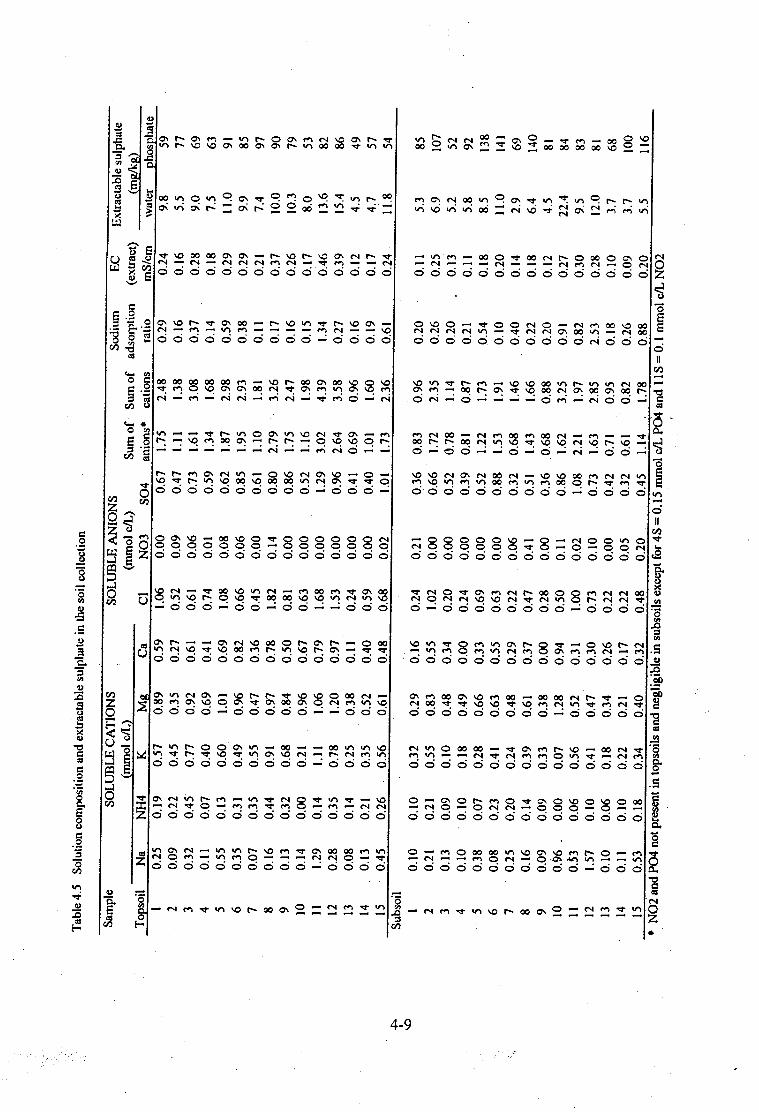
Tab

le 4

.5

Sol

utio

n co

mpo

siti

on a

nd e

xtra

ctab

le s

ulph

ate

in th

e so

il c

olle

ctio

n

Sam

ple

SO

LU

BL

E C

AT

ION

S

SO

LU

BL

E A

NIO

NS

S

odiu

m

EC

E

xtra

ctab

le s

ulph

ate

~mmol c/L~

(mm

ol c

/L)

Sum

of

Sum

of

adso

rpti

on

(ext

ract

) ~m

g/kB

) T

o2so

il

Na

NH

4 K

M

g C

a C

l N

03

S

04

an

ion

s•

cati

ons

rati

o m

S/c

m

wat

er

Eho

s2ha

te

I 0.

25

0.19

0.

57

0.89

0.

59

1.06

0.

00

0.67

1.

15

2.48

0.

29

0.24

9.

8 59

2

0.09

0.

22

0.45

0.

35

0.27

0.

52

0.09

0.

47

1.11

1.

38

0.1

6

0.16

5.

5 77

3

0.32

0.

45

0.77

0.

92

0.61

0.

61

0.0

6

0.73

1.

61

3.08

0.

37

0.28

9.

0 69

4

0.11

0.

07

0.40

0.

69

0.41

0.

74

O.o

t 0.

59

1.34

1.

68

0.14

0.

18

1.5

63

5 0.

55

0.13

0.

60

1.01

0.

69

1.08

0

.08

0.

62

1.87

2.

98

0.59

0.

29

11.0

91

6

0.35

0.

31

0.49

0.

96

0.82

0.

66

0.0

6

0.85

1.

95

2.93

0.

38

0.29

9.

9 85

7

0.07

0.

35

0.55

0.

47

0.36

0.

45

0.0

0

0.61

1.

10

1.81

0.

11

0.21

7.

4 97

8

0.16

0.

44

0.91

0.

97

0.78

1.

82

0.14

0.

80

2.79

3.

26

0.17

0.

37

10.0

90

9

0.13

0.

32

0.68

0.

84

0.50

0.

81

0.0

0

0.86

1.

75

2.47

0.

16

0.26

10

.3

79

10

0.14

0.

00

0.21

0.

96

0.67

0.

63

0.00

0.

52

1.16

1.

98

0.15

0.

17

8.0

53

11

1.29

0.

14

1.11

1.

06

0.79

1.

68

0.0

0

1.29

3.

02

4.39

1.

34

0.46

13

.6

82

12

0.28

0.

35

0.78

1.

20

0.97

1.

53

0.0

0

0.96

2.

64

3.58

0.

27

0.39

15

.4

86

13

0.08

0.

14

0.25

0.

38

0.11

0.

24

0.00

0.

41

0.69

0.

96

0.16

0.

12

4.5

49

14

0.13

0.

21

0.35

0.

52

0.40

0.

59

0.00

0.

40

1.01

1.

60

0.19

0.

17

4.7

51

15

0.45

0.

26

0.56

· 0.

61

0.48

0.

68

0.02

I.O

J 1.

73

2.36

0.

61

0.2

4.

11.8

54

~

Sub

soil

I \0

I

0.10

0.

10

0.32

0.

29

0.16

0.

24

0.21

0

.36

0.

83

0.96

0.

20

0.l

l 5.

3 85

2

0.21

0.

21

0.55

0.

83

0.55

l.

02

0.

00

0.66

1.

72

2.35

0

.26

0.

25

6.9

107

3 0.

13

0.09

0.

10

0.48

0.

34

0.20

0

.00

0.

52

0.78

1.

14

0.20

0.

13

5.2

52

4 0.

10

0.10

0.

18

0.49

0

.00

0.

24

0.0

0

0.3

9

0.81

0.

87

0.21

0.

11

5.8

92

5 0.

38

0.07

0.

28

0.66

0.

33

0.69

0

.00

0.

52

1.22

1.

73

0.5

4

0.18

8.

5 13

8 6

0.08

0.

23

0.41

0.

63

0.55

0.

63

0.0

0

0.8&

1.

53

1.91

0

.10

0.

20

11.0

14

1 ··;

; 7

0.25

0.

20

0.24

0.

48

0.29

0.

22

0.0

6

0.32

0.

68

1.46

0

.40

0.

14

2.9

69

8 0.

16

0.14

0.

39

0.61

0.

37

0.47

0.

41

0.51

1.

43

1.66

0.

22

0.18

6.

4 14

0 9

0.09

0.

09

0.33

0.

38

0.0

0

0.28

0

.00

0.

36

.0.6

8 0.

88

0.20

0.

12

4.5

81

10

0.96

.

0.00

0.

07

1.28

0.

94

0.50

0.

11

0.86

1.

62

3.25

0.

91

0.27

22

.4

84

11

o.53

0.

06

0.56

0.

52

0.31

1.

00

0.02

1.

08

2.21

1.

97

0.82

0.

30

9.5

83

12

1.57

0.

10

0.41

0.

47

0.30

0.

73

0.1

0

0.73

1.

63

2.85

2.

53

0.28

12

.0

81

13

0.10

0.

06

0.18

0.

34

0.26

0.

22

0.0

0

0.42

0.

71

0.95

0.

18

0.10

3.

7 6

8

14

0.11

0.

10

0.22

0.

21

0.17

0.

22

0.05

0.

32

0.61

0.

82

0.26

0.

09

3.7

100

15

0.53

0.

18

0.34

0.

40

0.32

0.

48

0.20

0.

45

1.14

'

1.78

0.

88

0.2

0

5.5

116

• N

02

and

P0

4 n

ot p

rese

nt in

tops

oils

and

neg

ligi

ble

in s

ubso

ils

exce

pt f

or 4

S =

0.15

mm

ol c

/L P

oi a

nd

11

S =

0. l

mm

ol c

/L N

02

'

4.3.2. Deposition gradients

A number of soil chemical parameters were plotted against distance from the power station

in order to establish whether any trends were evident. The relationship between distance and

some key properties which might be expected to vaJry with the intensity of atmospheric

pollution impacts, such as soil pH measured in water and various sulphur fractions (phosphate­

extractable sulphate, water-soluble sulphate and total sulphur) are shown in Figure 4.1.

Although no clear trends are evident, close inspection of Figure 4.1 b does show a decline in.

the concentration of water-soluble sulphate with distance. The high sulphate concentration in

the subsoil of site 10 (at 8.3 km from the power station) can be disregardeq because the soil

is unusually high in smectitic clay and therefore could be expected to accumulate solutes

compared with the other sites. The trend is probably not significant, but may demonstrate an

early indication of heightened water-soluble sulphate levels in the near-field of the power

station. The greatest concentrations are apparent about 4-6 km of the power station (excluding

site 10). As mentioned in Chapter 1, Section 1.5.1, Annegam et al. (1996) stated that high

S02 concentrations were unlikely to pose an environmental threat except within 4 km of a tall

stack. Turner (1992) predicted that plume touch down would occur at a distance of 2.5 km from a tall stack. Since the position of plume touch down is reliant on the local

meteorological conditions and the stack configuration such predictions cannot be broadly

applied. Nevertheless, the data in Figure 4.1 (b) suggest that heightened sulphate

concentrations are evident within 4-6 km of Arnot power station. The soluble sulphate

calculated as a fraction of the total dissolved solids in solution was also plotted against distance but no relationship was evident.

There was no evidence of heightened trace element concentrations in the vicinity of the powel'

station, supporting the prediction by Willis (1987), based on chemical data, that trace elements

from coal-burning power stations should not constitute an environmental problem.

4-10

a. b.

c.

1.S

7

-;:-6.S u c; ~ 6 ...... x

~ ::t: c..s.s

x

s co 4.S

0 s

160 ,..... .CQ

~140 0

e ........ u 120 a; 0 -= c. i JOO

~ x Q s 80 t)

e ~ 60 y x a.

40 0 s

Figure 4.1

2S ,.., ' co

0

I

0 }20 ...... 2 "' x °' 0 -g_1s

~ d = x

x x

"' x 0 ; O< c u 0 x xi ::0 10 x x > >o x 0 >i x ,.

~ 0

~ x ; )( i x O! 0 0 0

01 i!. s 0 d x x' 0

0 £ ~ 0

i 0

~ 0

0

JO IS 20 0 s 10 IS 20 Distance (km) Distance (km)

d.

6 '

I I 0

I

0

01 s x ,.....

"$. x ...... x x 34 x ' 0 .c

0 c. Gii 0 xi c x

~3 0 x 0 x! x 0 c s x 0 ~ x x '6

I o! x

~ x

1 0 0 0 0 >< 0 x 2 0

~ 0 x )

x ~ x : x 0 ; ; 0 i I

10 IS 20 0 s 10 IS 20 Distance (km) Distance (km)

Parameters plotted as a function of distance of sampling from the Arnot power

station a). pH(water), b). water-soluble sulphate c). phosphate-extractable

sulphate and d). total sulphur. Topsoils are indicated by a cross and subsoils by an open circle.

4.3.3. Parameters related to soil acidity

4. 3. 3.1. Soil pH

The suspension pH of each soil measured in water, KCl and K2S04 (Table 4.4) and the

relationships between these parameters are shown in Figure 4.2. The difference in pH

measured in water and pH in an electrolyte solution can be either positive, neutral or negative,

depending on the net charge on the soil colloids (Aitken and Moody, 1991). In all the soils

4-11

\

sampled, the relationship between these measures of pH followed the order pH(water) > pH(K2S04) > pH(KCl).

6

• 5.5

..-.-...... -~ tf)

5 "-"

::t 0..

4.5

4

4.5

Figure 4.2

pH (KCI) .... pH (K.2S04)

A. ... ... • ... ... ... ·•.a. ... -4 • • • • ... ...... ...... ....... - • ............ .... • ..... • • • • • . '

• .. • • - • ••••

5 5.5 6 6.5 7 7.5 pH (water)

Relationship of pH measured in KCI or K2S04 (pHsa1J to pH measured in water

for the 30 soils based on data in Table 4.4.

A comparison of pH values in salt solution shows a consistent difference of 0.4 to 0.6 pH

units between pH measured in KCl and pH in K2S04 • This linear relationship is strongly linear even in the low pH range (r=0.97, 28 degrees of freedom).

When the pH in salt solution is lower than in water, it is usually taken to indicate that

negative charge dominates the soil exchange surfaces (Parfitt,, 19~0). H+ and Al3"' ions ar.e

displaced from the negative exchange sites by the K+ ion, resulting in a decreasedpH relative

to that in water. In soils that are strongly sesquioxidic, on!y smaH reductions or even

increases in pH may result on the addition of salts - especially phosphate and sulphate salts.

-The anions exchange for Off from the positively charged sesquioxides resulting in a rise in

pH (Thomas and Hargrove, 1984). Accordingly, the gata in Figure 4.2 indicate that all the · s"oils have a net negative charge. Inspection of Figure 4.2 also reveals an apparent d~,parture from the general trend oflinearity in the low pH(water) range(< pH 5.5) for the relations~ps ofboth sulphate and chloride pH values with pH (water).

4-12

In the low pH range, the concentration of H+ in solution is already high and is therefore pH

is not as affected by the concentration of H+ released by the displacing salts. Consequently,

although pH may decrease in salt solution relative to that in water, the corresponding pH value

in salt solution is less depressed than at higher pH values - resulting in the curvilinear trend

at lower pH values (Figure 4.2). Aitken and Moody (1991) have demonstrated that the fitting

of a curvilinear function to similar data resulted in higher correlation coefficients than those

obtained for a linear fit. The difference in pH values measured in water and an electrolyte

solution also decreases as the pH decreases towards the pH value at which charge is no longer

generated on the soil surface, termed point of zero charge (PZC) (McBride, 1994; Sposito,

1989). The solution pH and the electrolyte concentration . determine the charge on

sesquioxide surfaces and whether these surfaces will adopt acidic or basic characteristics.

Figure 4.3 shows that the general trend is for LipH (i.e. pH(KCl) - pH( water)) to decrease with

decreasing pH - a phenomenon which Aitken and Moody ( 1991) indicate should be expected

for a suite of soils which possess variable charge but which are net negatively charged.

-0.8

-I

::r:: -1.2 c.. ~ -Q) 0 -1.4

-1.6

-1.8

4.5

Figure 4.3

o·

5

0 oo

Oo

5.5

x Topsoils o Subsoils

x 0 x xx xx x 0

0 ~~

0

oo 0

0 0

6 6.5 7 7.5 pH in water

Relationship between pH measured in water and LipH (i.e. pH(KCl)­

pH(water)), based on data in Table 4.4.

4-13

4. 3. 3. 2. Extractable acii!ily

The extractable or exchangeable acidity is measured as the moles of titratable protons per unit

mass displaced by an unbuffered KCl solution. For the soil collection, the exchangeable

acidity ranges between 0.3 and 10.6 mmolc.kg·1 (Table 4.4). The exchangeable acidity in soils

is primarily attributable to the readily exchangeable forms of Al3+ ions (Thomas and Hargrove,

1984; Sposito, 1989). The K+ ion replaces the Al species on the mineral surface, which then

hydrolyse in solution to re1ease protons which are measured as exchangeable acidity. In

Figure 4.4 the ratio of exchangeable acidity to effective cation exchange capacity (ECEC) is

plotted against pH in KCl, and the data clearly conform to the classical relationship between

acid saturation of the exchange surfaces and soil pH, described by Sposito (1989, p. 214).

6:15

frl 0.5 u ~ ,00.4 ·-"O ·o ~ C1) 0.3 -..0 ~ C1)

~0.2 ~ ..c u ><: ~ 0.1

0

4

•

Figure 4.4

•

• • ••• •

•• •

• • • • • . ... . ... - - -4.2 4.4 4.6 4.8 5

pH (KCI)

-5.2 5.4 5.6

The relationship between the acid saturation of the effective cation exchange

capacity (ECEC) and pH measured in KCI, based on data in Table 4;4

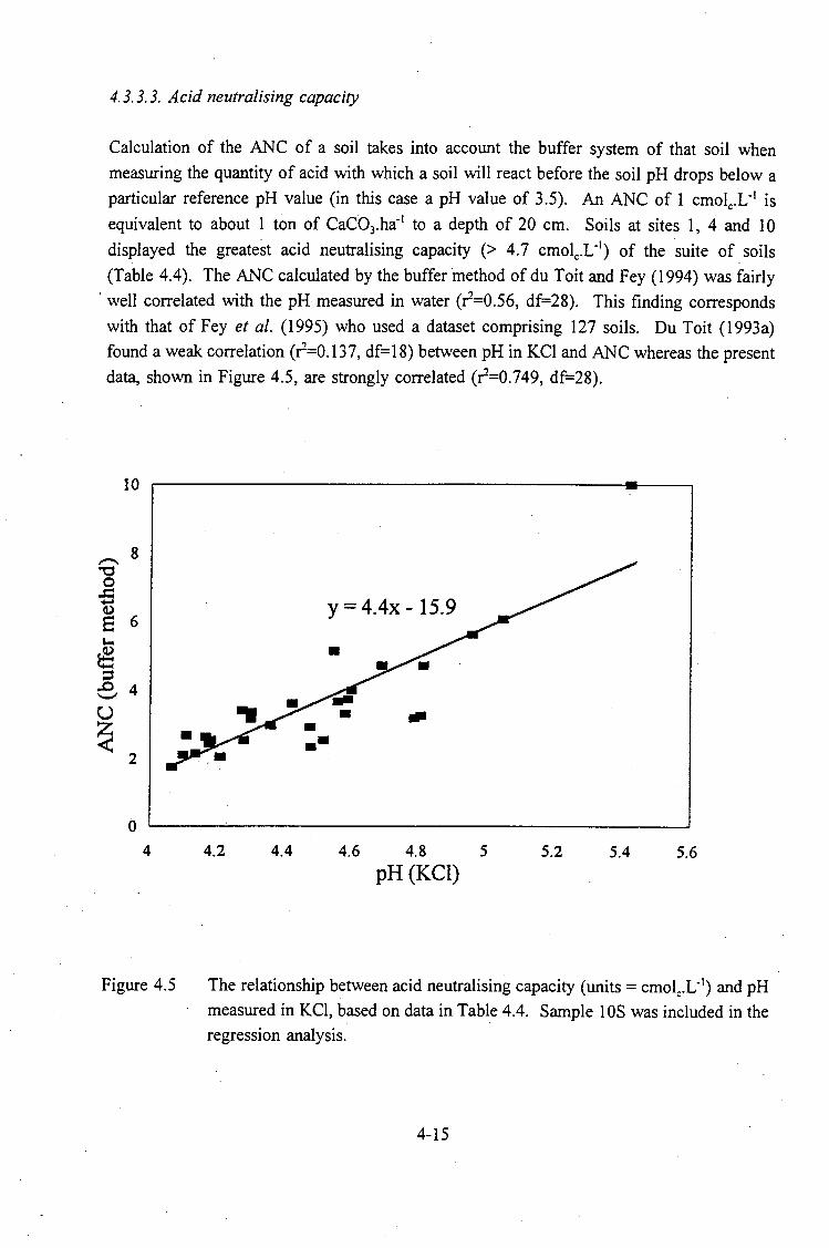
4.3.3.3. Acid neutralising capacity

Calculation of the ANC of a soil takes into account the buffer system of that soil when

measuring the quantity of acid with which a soil will react before the soil pH drops below a

particular reference pH value (in this case a pH value of 3.5). An ANC of 1 cmolc-L-1 is

equivalent to about 1 ton of CaC03.ha·1 to a depth of 20 cm. Soils at sites 1, 4 and 10

displayed the greatest acid neutralising capacity (> 4. 7 cmolc.L-1) of the suite of. soils

(Table 4.4). The ANC calculated by the buffer method of du Toit and Fey (1994) was fairly

·well correlated with the pH measured in water (r=0.56, df=28). This finding corresponds

with that of Fey et al. (1995) who used a dataset comprising 127 soils. Du Toit (1993a)

found a weak correlation (r=0.137, df=18) between pH in KCl and ANC whereas the present

data, shown in Figure 4.5, are strongly correlated (r=0.749, df=28).

10

,......... 8 "'O 0 ~ ._

<1) e 6 .... ~ ::t .0 4 '-" u ~

2

0

4

Figure 4.5

y = 4.4x - 15.9

•

...

4.2 4.4 4.6 4.8 5 5.2 5.4 5.6 pH (KCI)

The relationship between acid neutralising capacity (units= cmolc.L-1) and pH

measured in KCl, based on data in Table 4.4. Sample IOS was included in the

regression analysis.

4-15

According to van Breemen et al. (1983), the ANC of most soils is associated with silicate

minerals which have very slow dissolution kinetics. Van Breemen et al. (1983) used the

method of component composition to calculate the ANC of the soil, where the soil is

considered to include all inorganic matter including soil solution, solid particles and adsorbed

ions. ANC is calculated using total elemental analyses, but the method does not consider the

kinetics of mineral weathering. Nevertheless, du Toit (1993a) found significant relationships

between ANC calculated by component composition, serial titration with HCl and the ANC

buffer method described in Appendix 2. Of these methods, component composition was

selected as the least satisfactory method for comparison with the ANC buffer method. As a

consequence, ANC by component composition wa:s not calculated in the present study.

4.3.4. Soil sulphate

Sulphur compounds are the major atmospheric pollutants to which the soils in the vicinity of

Arnot are exposed, yet, as was demonstrated in Section 4.3.2, no relationships between the

various sulphur fractions and distance from the sulphur source are readily apparent. However~

Chapter 1 made clear that a number of factors influence the behaviour of sulphur, and in

particular sulphate, in soils. The capacity of soil to retain sulphate depends on factors such as the sesquioxide content, clay content and organic matter.

Fey and Guy (1993) suggested that the difference in pH measured in K2S04

and that measured

in KCl could be used as an easily measured index of the sulphate sorption capacity of soilg,,

The increased pH is supposedly related to the release of Off ions displaced by ligand

exchange with the sulphate anion (Curtin and Syers, l 990a). The sulphate anion is

specifically adsorbed in contrast to the indifferent chloride anion (Mott, 1981). The pH

difference (calculated as pH(K2S04) - pH(KCl)) should provide an indication of OH- release

which can be attributed to sulphate sorption. As is evident in Figure 4.6 there is no clear

relationship between this index of sulphate sorption and phosphate-extractable sulphate. However, there is a distinct separation of the topsoils from the subsoils. The small pH

difference manifested for the topsoils is attributable to the greater organic matter content in

the topsoil horizons. In the lower horizons, there is a lower concentration of humic substances

to block positively charged sites on the sesquioxide surfaces. As is apparent in Figure 4.6,

the pH difference between pH measured in K2S04 and that measured in KCl would not serve as a reliable indicator of phosphate-extractable sulphate.

4-16

160 ,-... CJ)

~140 E ........,

2 120 ce ..c c.. -~ 100 0 -.,0 ce 80 ... 0 ce .... ... >(

60 0

~

40

0.35

Figure 4.6

x Topsoil 0 Subsoil 0 0 0

0

0

x 0

x x 0 x x og 0 x 0 x x

x 0 0 x x x x x 0 x

0.4 0.45 0.5 0.55 0.6 0.65

Difference in pH (sulphate - chloride)

The relationship between difference in pH(K2S04 - KCl) and phosphate­

extractable sulphate based on data presented in Tables 4.4 and 4.5.

The relationships between both water- and phosphate-extractable sulphate and a number of

other soil properties known to influence sulphate sorption were also explored. Parameters

included clay and, specifically, kaolinite content, CBD-extractable Mn, Fe and Al, organic

carbon, ANC, acid saturation and ECEC, as well as pH in water, KCl and K2S04• No clear

relationships or correlations were apparent between any of these individual parameters and the

various sulphate fractions. Although the dependence of sulphate sorption on soil properties

such as sesquioxide content and pH is theoretically apparent, these relationships are not simple

linear functions. Sulphate retention would appear to depend more on the interplay between

the various factors. For this reason an attempt was made to derive an expression which relates

the various factors to one another in such a way as to provide an estimate of extractable

sulphate. Such an expression might be termed a sulphate r~tention index. An example of such

an index is plotted against extractable sulphate in Figure 4. 7. Factor weightings were chosen

based on an intuitive estimate· of the relative importance of each factor in contributing (either positively or negatively) to the retention of sulphur in soil.

4:.17

The sulpbate retention index was calculated as follows:

SRI = kaolinite content + S(F e content) - I 0( organic carbon content)

160 -. OJ)

.~140 E ...._, 2 120 ~ ..c c.. ~ 100

CL> -~ - ·80 0 e -~ 60

~

40

-30

Figure 4.7

where tbe contents are expressed as %. Kaolinite is calculated from the clay

content and the % kaolinite in 'the day fraction (by XRD) while the Fe content

is that extracted with citrate-bicarbonate-dithionite.

x Topsoils o Subsoils 0 0

x

,Q

' 0

0

x 0

x x 0 0 x .c9oo x

x cO x xx

0 x x

x

-20 -10 0 10 20 30

Sulphate retention index

The relationship between the index of sulphate retention (SRI) and phosphate­

extractable sulphate.

Figure 4. 7 shows a clear separation of topsoils from subsoils - primarily on the basis of

organic matter content. The subsoil 1 OS is an exception as, as stated previously, it is

characterised by a smectitic mineralogy. The calculated SRI for the subsoils considered

separately, demonstrates a linear relation {r2 = 0.68, df = 12, IOS excluded from regression

calculation) with the phosphate extractable sulphate. For the subsoils, the equation of the line

'is: P-extractable sulphate = 4.3(SRI) + 53. There is no relationship evident for the topsoils.

The topsoils and subsoils (except the smectitic 1 OS) are fortuitously separated into positive and

negative sectors, with topsoils being sulphate-repelling and subsoils sulphate-retaining.

4-18

Although this index is a crude estimate of the relative importance of the factors influencing

sulphate retention, it could be further developed into a potentially useful tool for the

assessment of geochemical responses to atmospheric pollution impacts. Changes in either the

slope or intercept or both, of the relationship between extractable sulphate and the subsoil SRI,

could provide some indication of an accumulation of sulphate which might be more reliable

than extractable sulphate alone. Such comparisons may not only facilitate the assessment of

sulphate accumulation but also may prove useful in comparing sites in different regions of the sub-continent.

The importance of organic carbon in governing sulphate accumulation in soils has been

implicitly demonstrated in both Figure 4.6 and 4. 7. Organic carbon is widely recognised as

being negatively correlated with extractable sulphate (Comfort et al.~ 1992 and references cited

in Section 1.7.3.) To a certain extent this assertion is supported by the present data, as shown

in Figure 4.8. Again, the separation between topsoils and subsoils on the basis of organic

matter is evident. The higher organic carbon fractions in the topsoil horizons imply a greater

proportion of humic substances which compete with sulphate for sorption sites. Sulphate that

is not bound to the soil surface is lost through leaching, resulting in a low extractable sulphate

fraction. The data conform to the generalisation made by Tisdale et al. (1985) that there is

an accumulation of adsorbed SO/" in deeper soil horizons - supposedly as a result of

eluviation or leaching of sulphates from the upper horizons.

160

""" 00

~140 E "-'

£ 120 C':S ..c c.

] 100 C) -.D s 80 0 C':S '-..... ~ 60

40

0

Figure 4.8

0

0 8 x Topsoils o Subsoils

0

0 0 x

0 x x 0 @ x x

0 0 x x co x

x x x x x x

1 2 3 4 5 Organic carbon (%)

Phosphate-extractable sulphate as a function of soil organic carbon, based on data in Tables 4.1 and 4.5.

4-19

Conversely, there is a weak but pos1t1ve relationship between organic carbon and the

concentration of water-soluble sulphate in the soil solution, shown in Figure 4.9 (r = 0.29;

df=27). This result is not unexpected as organic matter will enhance the desorption and thus

the solubility of sulphate. The outlier represented by the subsoil of site 10 was excluded in

the calculation of the regression. The quantities of soluble sulphate in soils fluctuate

seasonally and on a year-to-year basis. The variation is a consequence of the interaction

between environmental and seasonal factors on the mineralization of organic sulphur, the

fluxes of soil moisture and sulphate uptake by plants. · When plant and animal residues are

returned to the soil, microbial metabolism is responsible for converting the organically bound

sulphur to sulphate (Tisdale et al., 1985). Most of the sulphur remains organically bound in the soi1 humus.

25 ,-.... tlO

~20 e . ......., Cl) (d .g_ 15 -::s en a.> -10 ~ -0 {/)

~ 5 C1)

(d

~ 0

0

Figure 4.9

.,

0 x Topsoils 0 Subsoils . ,;

.

· .. x

x 0 x x 0 x x x x 9< 0 ·x

x x 0 0 Oet-0 0 0 ~

o®

l 2 3 4 5

Organic carbon(%)

Relationship between water-soluble sulphate and organic C, based on data in Tables 4.1 and 4;5.

Tabatabai (1982) stressed the importance of organic matter in influencing the amount and

form in which sulphur occurs in the soil. A strong relationship (r=0.85, df=27) (Figure 4.10)

exists between the fraction of organic carbon present in soil and the total sulphur content of

the soil, confirming that the greatest fraction of sulphur in the soil is usually organically

bound. Tisdale et al. ( 1985) state that in excess of 90 % of the sulphur in noncalcareous soils

4-20

exists in organic form. In Figure 4.10 the y-intercept represents the sulphur in the soil that

is not in association with organic matter. Background levels of sulphur in ·soils can be

attributed to S-bearing minerals in the parent rock. The parent material in the Arnot area

could be high in sulphide-bearing minerals such as pyrite. This hypothesis is tentatively

supported by the unpublished data (Willis, pers. comm:) for the sulphur content of coal from

the Arnot coal seams. The number I seam has an S-content of 2.0 % while the number 2

seam bears 1.1 % sulphur. These values exceed or approach the upper limit of the reported

range for South African coal ((0.4 - 1.4 %; Willis, 1983). Thus it is feasible that the soils in

the vicinity have inherited a high sulphur content from the parent material. In the long-term,

however, most of this additional sulphur would be expected to become incorporated pedogenically in the humus fraction.

Jacks et al. (1994) traced sulphur sources in soils and waters using sulphur isotope ratios and

concluded that the mobilisation of sulphur through bedrock weathering is negligible. Jacks

et al. (1994) studied gneisses and charnockites and whether their results are applicable to teh

shales and dolerites of the Arnot area is an aspect that requires further investigation.

500 • •

r--.. y= 7.8 x + 129 • OD • ~ 400

E I ~

'"" _g 300 0... • -::s ti) -~ 0 200 • ~

• • • • 100

0 10 - 20 30 40 50 Organic carbon (mg/kg)

Figure 4.10 Relationship between total S and organic C -for the soil collection, based on

data from Tables 4.1 and 4.2. The regression was performed without the outlier (I OS), giving an r2 of 0. 73 (df=27).

4-21

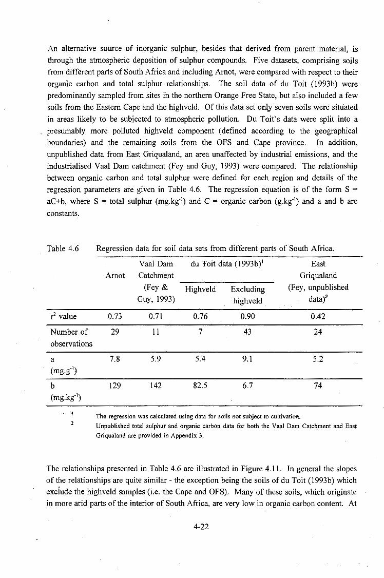
An alternative source of inorganic sulphur, besides that derived from parent material, is

through the atmospheric deposition of sulphur compounds. Five datasets, comprising soils

from different parts of South Africa and including Arnot, were compared with respect to their

organic carbon and total sulphur relationships. The soil data of du Toit (1993b) were

predominantly sampled from sites in the northern Orange Free State, but also included a few

soils from the Eastern Cape and the highveld. Of this data set only seven soils were situated

in areas likely to be subjected to atmospheric pollution. Du Toit's data were split into a

presumably more polluted highveld component (defined according to the geographical

boundaries) and the remaining soils from the OFS and Cape province. In addition,

unpublished data from East Griqualand, an area unaffected by industrial emissions, and the

industrialised Vaal Dam catchment (Fey and Guy, 1993) were compared. The relationship

between organic carbon and total sulphur were defined for each region and details of the

regression parameters are given in Table 4.6. The regression equation is of the form S = aC+b, where S = total sulphur (mg.kg-1

) and C = organic carbon (g.kg-1) and a and b are

constants.

Table 4.6 Regression data for soil data sets from different parts of South Africa.

Vaal Dam du Toit data (1993b) 1 East

Arnot Catchment Griqualand

(Fey & Highveld Excluding (Fey, unpublished

Guy, 1993) highveld data)~

r2 value 0.73 0.71 0.76 0.90 0.42

Number of 29 11 7 43 24

observations

a 7.8 5.9 5.4 9.1 5.2 (mg_g-')

b 129 142 82.5 6.7 74 (mg.kg-1)

"' The regression was calculated using data for soils not subject to cultivatioft. 2 Unpublished total sulphur and organic carbon data for both the Vaal Dam Catc~ment and East

Griqualand are provided in Appendix 3.

The relationships presented in Table 4.6 are illustrated in Figure 4.11. In general the slopes

of the relationships are quite similar - the exception being the soils of du Toit (1993b) which

exciude the highveld samples (i.e. the Cape and OFS). Many of these soils, which originate

in more arid parts of the interior of South Africa, are very low in organic carbon content. At

4-22

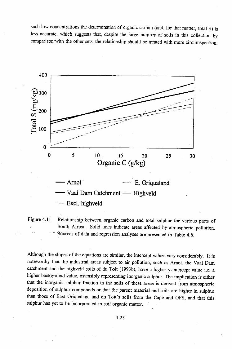
such low concentrations the determination of organic carbon (and, for that matter, total S) is

less accurate, which suggests that, despite the large number of soils in this collection by

comparisonwith the other sets, the relationship should be treated with more circumspection.

400

...-. 0.0 300

~ e ~100 r.I'.)

...... ~ ~

0 100 ~

0

0 5 10 15 20 25 30 Organic C (g/kg)

-Arnot -·········· E. Griqualand

- Vaal Dam Catchment - Highveld

--·-··-· Exel. highveld

Figure 4.11 Relationship between organic carbon and total sulphur for various parts of

South Africa. Solid lines indicate areas affected by atmospheric pollution.

• - -Sources of data and regression analyses are presented· in Table 4.6.

Although the slopes of the equations are similar, the intercept values vary considerably. It is

noteworthy that the industrial areas subject to air pollution, such as Arnot, the V aal Dam

catchment and the highveld soils of du Toit (1993b), have a higher y-intercept value i.e. a

higher background value, ·ostensibly representing inorganic sulphur. The implication is either

that the inorganic sulphur fraction in the soils of these areas is derived from atmospheric

deposition of sulphur compounds or that the parent material and soils are higher in sulphur

than those of East Griqualand and du Toit's soils from the Cape and OFS, and that this sulphur has yet to be incorporated in soil organic matter.

4-23

Before any conclusions can be drawn concerning these findi1'gs, more extensive information

on the composition of the parent material is required, particularly with reference to the

sulphur-bearing mineral component. In addition, data sets from other parts of southern Africa

should be established and the relationships between organic carbon and total sulphur

compared. Nevertheless, the data presented above suggest that soils subject to atmospheric

deposition of sulphur compounds may possess a higher inorganic sulphur component than soils unaffected by atmospheric pollution.

Although the relationship between carbon and sulphur in the organic fraction falls within a

fairly narrow range, Tisdale et al. (1985) report marked differences between the C/N/S ratios

among and between types of world soils. Such variation is attributable to variations in parent

material and other soil-forming factors such as climate, drainage and vegetation. A close

association· is reported for the sulpnur and nitrogen components of soil organic matter thus

Tisdale et al. (1985) suggest that total nitrogen and organic sulphur are more closely

correlated than organic carbon and organic sulphur. The C:S ratio for humins, humic acids

and fulvic acids range between 36 to 145 whereas the N:S ratio ranges between 2.7 to 8.3

(Sparks, 1995). Since the N/S ratio in most whole soils falls within the narrow range of 6 to

8:1 (Tisdale et al., 1985) the relationship between nitrogen and sulphur may be a more

valuable one to utilize in the quest for indications of sulphur deposition from atmospheric pollution.

4-24

4.4. Conclusions

The soils in the vicinity of Arnot power station are moderately acidic sandy-loams or loamy­

sands. The soils are variably-charged, dominated by negative charge. Kaolinite is the

dominant mineral in the clay fraction with the exception of the site 10 soil which has an equal

proportion of smectite. In all the soils, Fe dominates the sesquioxidic fraction.

No trends in major or trace elements with distance from the power station were apparent.

Measures of pH in water, KCl and K2S04 as well as phosphate-extractable sulphate against

distance showed no relationships. Water-soluble sulphate is an exception as it appears to be

elevated within 6 km of the power station.

Since sulphate retention on soil depends on a combination of factors such as soil pH and

sesquioxide content rather than a single factor, two indices of sulphate retention were

explored. An index of sulphate retention calculated from the pH difference between pH

measured in KCI and that in K2S04 did not show a correlation with the phosphate-extractable

sulphate, although the subsoils and topsoils were separated into two distinct groups. A

sulphate retention index calculated as [kaolinite content + 5(Fe content) - I 0( organic carbon

content)] not only separated topsoils from subsoils but revealed a linear relationship between

phosphate-extractable sulphate and the SRI for the subsoils. No relationship was apparent for

the topsoils which suggests that the relatively high concentration of humic substances in the

topsoils blocks the sorption of sulphate on the sesquioxide surfaces.

The presence of organic matter in soil is acknowledged to play an important role in sulphate

retention. The relationships between organic carbon and total sulphur were therefore explored

for five areas, two of which are relatively unaffected by emissions from industrial activity.

Preliminary findings suggest that inorganic sulphur levels are higher in areas affected by

atmospheric deposition compared with areas in which no atmospheric pollution from industry

is apparent. Further investigation to isolate the contribution from the parent material and that

hypothesized to originate from atmospheric deposition is strongly recommended. The

relationship between nitrogen and total sulphur could be used rather than organic carbon and

total sulphur as the N:S ratio is apparently more narrowly defined. In the long-term, a change

in the N:S relationship may reflect whether or not sulphur is accumulating as a consequence

of atmospheric deposition.

4-25

GENERAL DISCUSSION AND CONCLUSIONS

The thirty soils collected during the course of this study provide a baseline data set for long­

term monitoring of atmospheric deposition impacts to soils. The geographical co-ordinates

of each site which was sampled are provided and site features are described to facilitate

resampling in the future. Soil samples collected during the present study are stored at two

locations in South Africa and will provide historical samples for future comparison. A

preliminary attempt to test the repeatability of the sampling protocol suggests that a more

rigorous approach should be adopted. Ramsey et al. (1995) provide guidelines for statisticaIIy

valid tests of the repeatability and reproducibility of sampling protocols.

Of all the analytical techniques employed in this study, only the determination of phosphate­

extractable. sulphate was critically investigated. The use of turbidimetry for accurate

determination of phosphate-extractable sulphate is questionable as the high phosphate

concentration required to displace sulphate from the exchange sites interferes with the

determination. Although generally considered inappropriate, ion chromatography is suggested

as a viable alternative to turbidimetry for the determination of phosphate-extractable sulphate.

The relationships between soil chemical features and the amount of sulphate sorbed on soil

surfaces were investigated. An index of sulphate retention, calculated as [kaolinite + 5(Fe

content) - IO( organic carbon content)], was found to give a satisfactory separation of topsoils

from subsoils. The relationship between the sulphate retention index and phosphate-extractable

sulphate was found to be linear for the subsoils only, suggesting that once the competition for

positively charged sites from organic matter is reduced, sulphate retention is controlled by the

free Fe oxide and kaolinite contents of the clay fraction.

Preliminary results suggest that evidence of impacts of atmospheric deposition may be

appearing in the soils near Arnot power station. Arnot has been burning fossil fuels for·

electricity production since 1971, and there is an indication that concentrations of water­

soluble sulphate may be elevated in the soils near the power station. The highest

concentrations of water-soluble sulphate (13.6 - 15.4 mg.kg-1) were found within 4-6 km of

the power station. However, sampling was only conducted in an arc extending ENE to SE

of the power station as this area was assumed to be most frequently subjected to looping

pollution plumes. Efforts to verify these results should focus on an area upwind of the

prevailing wind direction and should sample soils. beyond 20 km of the power station to

establish more reliable background values of water-soluble sulphate in the local soils. Apart

from water-soluble sulphate there is no indication of a deposition gradient for any of the trace

elements, the major elements or parameters linked to soil acidity.

xii

The relationship between total sulphur and organic carbon described for the soils in the

vicinity bf Arnot suggests an elevated background concentration of inorganic sulphur compared

with soils from regions likely to be less polluted. The relationships derived for soils

originating in supposedly polluted areas (the Vaal Dam catchment, highveld soils and the

immediate surrounds of Arnot power station) generally revealed a higher background

concentration of inorganic sulphur than that derived for soils of unpolluted regions {East

Griqualand, Eastern Cape and Orange Free State). Whether this inorganic sulphur is a legacy

of the parent material or a consequence of atmospheric deposition of sulphur compounds is

an aspect that requires further research. Further research should focus on gathering data from

various regions of southern Africa to establish whether background levels of inorganic sulphur

can be attributed to atmospheric deposition of sulphur compounds or to the parent material.

Additional work is required to assess whether total nitrogen would prove more suitable than

organic carbon in establishing background inorganic sulphur concentrations, as the N :S ratio

is generally more restricted than the C:S ratio.

The evidence so far suggests that long-term monitoring of soil chemistry in the vicinicy of

Arnot power station is essential. Long-term monitoring will permit impacts to be detected at

a reasonably early stage and allow the timely implementation of appropriate control strategies.

To this end the establishment of a reliable monitoring system, in which both the sampling and

analytical techniques employed are repeatable and accurate, is imperative. In particular, a

study of the manner in which the interrelationships between parameters, rather than simply the

parameters themselves, are altered, could prove fruitful in the detection of impacts of atmospheric pollution on the pedosphere.

Xlll

REFERENCES

Adams T McM and.PW Lane, 1984. A comparison of four methods of analysing aqueous soil extracts for sulphate. J Sci. Food Agric. 35:750-744.

Aitken RL and PW Moody, 1991. Interrelations between soil pH measurements ion various

electrolytes and soil solution pH in acidic soils. Aust. J Soil Res. 29:483-491.

Alewell C, Manderscheid B, Li.ikewill A, Koeppe P and J Prenzel, 1995. Describing soil SO/­

dynamics in the Solling Roof Project with two different modelling approaches. Water Air Soil Pollut. 85:1801-1806.

Alloway BJ, 1995. Chapter 2 - Soil processes and the behaviour of metals. In: Alloway BJ

(Ed) Heavy metals in soils (Second edition). Blackie Academic. London. 368pp.

American Public Health Association, 1971. Standard methods for the examination of water

and wastewater. Greenberg AE, Trussell RR and LS Clesceri (Eds). American Public Health Association, Washington DC. 1268pp.

Annegam HJ, Turner CR, Helas G, Tosen GR and RP Rorich, 1996. Chapter 6 - Gaseous

pollutants. In: Held G, Gore BJ, Surridge AD, Tosen GR, Turner CR and RD

Walmsley (Eds). Air pollution and its impacts on the South African Highveld

Environmental Scientific Association, Cleveland, 144pp.

Ayers GP, Gillett RW, Selleck PW and ST Bentley, 1995. Rainwater composition and acid

deposition in the vicinity of fossil fuel-fired power plants (5550 MW total generating

capacity) in southern Australia. Water Air Soil Pollut. 85:2313-2318.

Bansal KN and AR Pal, 1987. Evaluation of a soil test method and plant analysis for

determining the sulphur status of alluvial soils. Plant Soil 98:331-336.

Bansal KN, Motiramani DP and AR Pal, 1983. Studies on sulphur in Vertisols. I. Soil and

plant tests for diagnosing sulphur deficiency in soybean (Glycine max (L.) Merr.). Plant Soil 70:133-140. (Cited in Bansal and Pal, 1987).

Bell N, 1996. Reports prepared by international delegates. Workshop on the impacts of air

pollution on the quality of soil and water: a southern African perspective, Johannesburg, 22-23 August 1996. Project No. 7760Tl27R. Eskom, Johannesburg.

Bennet M 1995. A Lidar study of the limits to buoyant plume rise in a well-mixed boundary layer. Atmos. Environ. 29(17):2275-2288. (Cited in Fey et al., 1996)

xiv

Bolan NS, Syers JK and RW Tillman, 1986. Ionic strength effects on surface charge and

adsorption of phosphate and sulphate by soils; J Soil Sci. 37:379-388.

Brimblecombe P, 1986. Air composition and chemistry. Cambridge University Press, Cambridge. 224pp.

Brodin YW and JCI Kuylenstierna, 1992. Acidification and critical loads in Nordic countries: a background. Ambio 21(4):332-338.

Buhmann C, 1986. Investigation of 2: 1 layer silicate clays in selected southern African soils.

PhD Thesis. Department of Soil Science and Agrometeorology, University of Natal, Pietermaritzburg.

Charlson RJ, Anderson TL and RE McDuff, 1992. The sulphur cycle. In: Global

biogeochemical cycles. Butcher SS, Charlson RJ, Orians GH and GV Wolfe (Eds.) Academic Press, London. 3 79pp.

Chief Directorate: Surveys and Land Information, 1987. 2529DD Arnot, 1 :50 000 topocadastral map, second edition.

Claisse F and JP Willis, 1995. Chapter 12A - Glass discs and solutions by borate fusion. In:

Willis JP (Ed) 1996. Course on theory and practice of XRF spectrometry. Department

of Geological Sciences, University of Cape Town, South Africa.

Comfort SD, Dick RP and J Baham, 1992. Modeling soil sulpate sorption characteristics. J Environ. Qua!. 21 :426-432.

Courchesne F, Gobran GR and A Dufresne, 1995. The role of humic acid on sulphate

retention and release in a podzol. Water Air Soil Pollut. 85:1813-1818.

Curtin D and JK Syers, 1990a. Mechanism of sulphate adsorption by two tropical soils. J Soil Sci. 41 :295-304.

Curtin D and JK Syers, 1990b. Extractability and adsorption of sulphate in soils. J Soil Sci. 41:305-312.

Du Toit B, 1993a. Soil acidification under forest plantations and the determination of the

ANC of soils. MSc Thesis. Faculty of Agriculture, University of Natal, Pietermaritzburg. 90pp.

xv

Du Toit MC, l 993b. Effek van bewerking op die swawelfraksise m geselekteerde

droelandgronde. MSc Thesis. Faculty of Agriculture, University of the Orange Free State. 141 pp.

Du Toit B and MV Fey, 1994. A simple test for the acid neutralising capacity of soils.

International Society of Soil Science and Mexican Society of Soil Science. ISBN 968-6201-25-4.

Duncan AR, Erlank AJ and PJ Betton, 1984. Analytical techniques and database descriptions.

Spec. Pub!. Geol. Soc. S. Afr. 13, Appnedix 1:389-395. (Cited in Willis, 1996).

Eskom, 1995. Statistical yearbook - 1995. Eskom Communication Services. Megawatt Park, Sandton, South Africa.

Falkengren-Grerup U, Linnermark N and G Tyler, 1987. Changes in acidity and cation pools

of South Swedish soils between 1949 and 1985. Chemosphere 16 (10-12):2239-2248.

Fey MV and SA Guy, 1993. The capacity of soils of the Vaal Dam catchment to retain

sulphate from atmospheric pollution. Report to the Water Research Commission by the

Department of Agronomy, University of Natal, Pietermaritzburg. WRC Report No 414/1/93. 90pp.

Fey MV and AA Netch, 1996. Chapter 15 - Impacts on the pedosphere. In: Held G, Gore

BJ, Surridge AD, Tosen GR, Turner CR and RD Walmsley (Eds). Air pollution and its

impacts on the South African Highveld. Environmental Scientific Association, Cleveland, l 44pp.

Fey MV, Nowicki TE and HA Dodds, 1995. Sensitivity of the soil environment to the· deposition of acidifying air pollutants in South Africa. . Confidential Report no TRR/S95/20 libs. Eskom Technology Group.

Fey MV, Nowicki TE and HA Dodds, 1996. Sensitivity of the soil environment to the

deposition of acidifying air pollutants in South Africa. Confidential Report no TRR/S96/209. Eskom Technology Group.

Fifield FW, 1995. Chapter 5 - Separation techniques. In: Fifield FW and PJ Haines (Eds.)

Environmental analytical chemistry. Blackie Academic and Professional, London, 424 pp.

Fox RL, Olson RA and HF Rhoades, 1964. Evaluating the sulphur status of soils by plants

and soil tests. Soil Sci. Soc. Am. Proc. 28:243-246. (Cited in Tabatabai, 1982).

XVI

Fox RL, Hue NV and AJ Parra, 1987. A turbidimetric method for determining phosphate­

extractable sulphates in tropical soils. Commun. Soil Sci. Plant Anal. 18:343-357. (Cited in MC du Toit, 1993)

Freedman B and TC Hutchinson, 1980. Pollutant inputs from the atmosphere and

accumulations in soil and vegetation near a nickel-copper smelter at Sudberry, Ontario,

Canada. Can. J Bot. 58:108-132. (Cited in Fey MV, Nowicki TE and HA Dodds., 1996.

Sensitivity .of the soil environment to the deposition of acidifying air pollutants in South

Africa. Confidential Report no TRR/S96/209. Eskom Technology Group.)

Freney JR, 1961. Some observations on the nature of organic sulphur compounds in soils.

Aust. J Agric. Res. 12:424-432. (Cited in Tabatabai, 1982).

Freney JR and CH Williams, 1983. Chapter 3 - The sulphur cycle in soil. In: Ivanov MV

and JR Freney (Eds.) The global biogeochemical sulphur cycle. SCOPE/UNEP

Workshop 19. John Wiley and Sons, Chichester. 470pp.

Galloway JN, Likens GE and ES Edgerton, 1976. Acid precipitation in the northeastern

United States: pH and acidity. Science 194:722-724.

Giesler R, Moldan F, U Lundstrom and H Hultberg, 1996. Reversing acidification in a

forested catchment in southwestern Sweden: effects on soil solution chemistry. J Environ. Qua!. 25: 110-119.

Gnoinski J, Tullmin MAA and M Nixon, 1996. Chapter 16 - Monitoring of atmospheric

corrosion in the Mpumalanga highveld. In: Held G, Gore BJ, Surridge AD, Tosen GR,

Turner CR and RD Walmsley (Eds). Air pollution and its impacts on the South African

Highveld. Environmental Scientific Association, Cleveland, l 44pp.

Guggenberger G and W Zech, 1992. Retention of dissolved organic carbon and sulphate in

aggregated acid forest soils. J Environ. Qua!. 21 :643-653.

Gustafsson JP, 1995. Modelling pH-dependent sulphate adsorption in the Bs horisons of

podsolized soils. J Environ. Qua!. 24:882-888.

Guadalix ME and MT Pardo, 1991. Sulphate sorption by variable charge soils. J Soil Sci. 42:607-614.

Handbook of standard soil testing methods for advisory purposes, 1990. Prepared by the non­

affiliated soil analysis work committee. Soil Science Society of South Africa, Pretoria.

xvu

Hedin LO, Granat L, Likens GE, Buishand TA; Galloway JN, Butler TJ and H Rodhe, 1994.

Steep declines in atmospheric base cations in regions of Europe and North America. Nature 367:351-354.

Heinrich KF J, 1986. Mass absorption coefficients for electron probe microanalysis. In: Proc.

11th Int. Congress on X-ray Optics and Microanalysis, London, Canada. Brown JB and RH Packwoods (Eds.) (Cited in Willis, 1996).

Held G, Annegarn HJ, Turner CR, Scheifinger H and GM Snyman, 1996a. Chapter 7 -

Atmospheric particulates, aerosols and visibility. In: Held G, Gore BJ, Surridge AD,

Tosen GR, Turner CR and RD Walmsley (Eds). Air pollution and its impacts on the

South African Highveld. Environmental Scientific Association, Cleveland, l 44pp.

Held G, Scheifinger H, Snyman GM, Tosen GR and M Zunckel, 1996b. Chapter 9 - The

climatology and meteorology of the Highveld. In: Held G, Gore BJ, Surridge AD,

Tosen GR, Turner CR and RD Walmsley (Eds). Air pollution and its impacts on the

South African Highveld. Environmental Scientific Association, Cleveland, 144pp.

Held G, Pienaar JJ, Snyman GM, Osborne J, Lachmann G and CR Turner, 1996c. Vertical

distribution of atmospheric particulates and water soluble pollutants over the highveld.

National Association for Clean Air Conference Proceedings, November 1996, Mpumalanga.

Hogan GD and DL Wotton, 1984. Pollutant distribution and effects in forests adjacent to

smelters. J Environ. Qua!. 13(3):377-382.

Inskeep WP, 1989. Adsorption of sulphate by kaolinite and amorphous iron oxide in the

presence of organic ligands. J Environ. Qua!. 18:379-385.

Jacks G, Sharma VP, Torssander P and G Aberg, 1994. Origin of sulphur in soil and water

in a Precambrian terrain, S. India. J Geochem. 28:351-358.

Jackson ML and GD Sherman, 1953. Chemical weathering of minerals in soils. In: AG

Norman (Ed.) Adv. in Agron. 5. Academic Press, New York. pp 221-317. Cited in McBride, 1994).

Jackson ML, Lim CH and L W Zelazny, 1986. Oxides, hydroxides and aluminosilicates. In:

Methods of soil analysis, Part 1. Physical and mineralogical methods - Agronomy

Monograph No. 9 (2nd edition) Soil Science Society of America. 1188pp.

xviii

Johnson DW, Lindberg SE and LF Pitelka, 1992. Chapter 1 - Introduction. In:Johnson DW

and SE Lindberg (Eds.) Atmospheric Deposition and Forest Nutrient Cycling. Ecological Studies 91. Springer-Verlag, New York. 707pp.

Johnson CM and H Nishita, 1952. Microestimation of sulphur in plant materials, soils and

irrigation waters. Anal. Chem. 24:736-742. (Cited in Tabatabai, 1982).

Jyla K, 1995. Deposition around a coal-fired power station during a wintertime precipitation event. Water Air Soil Pollut. 85:2125-2130.

Kashulina G, Jevtjugina Z and P de Caritat, 1995. Soil acidity status in the vicinity of the

Severonickel smelter complex (Kola Peninsula, Russia). Acid Reign Conference '95 Abstract book. In press: Water Air Soil Pollut. 85(1-4).

Kohnke H, 1968. Chapter 3 - Mechanical composition of the soil. Soil Physics. McGraw­Hill Book Co. New York. 224pp.

Kempster PL, Skoroszewski RW, Roos GN and BJ Gore, 1996. Chapter 14 - Impact of

atmospheric deposition on water quality. In: Held G, Gore BJ, Surridge AD, Tosen GR,

Turner CR and RD Walmsley (Eds). Air pollution and its impacts on the South African

Highveld. Environmental Scientific Association, Cleveland, l 44pp.

Kooner ZS, Jardine PM and S Feldman, 1995. Competitive surface complexation reactions

of sulphate and natural organic carbon on soil. J. Environ. Qua!. 24:656-662.

Koptsik G and I Mukhina, 1995. Effects of acid deposition on acidity and exchangeable

cations in podzols of the Kola Peninsula. Water Air Soil Pollut. 85:1209-1214.

Kuylenstierna JA, 1996. Reports prepared by international delegates. Workshop on the­

impacts of air pollution on the quality of soil and water: a southern African perspective, Johannesburg, 22-23 August 1996. Eskom Project No. 7760Tl27R.

Kuylenstierna JA, Cambridge H, Cinderby S and MJ Chadwick, 1995. Assessing the

sensitivity of ecosystems to acidic deposition in developing countries. Acid Reign '95

Conference Proceedings Abstract Book. In press: Water Air Soil Pollut. 85(1-4).

Land Type Memoirs 2528 Pretoria, 1987. Memoirs on the agricultural natural resources of

~outh Africa No. 8. The Department of Agriculture and Water Supply, Republic of South Africa.

Li T-Y and HE Lands~erg, 197 5. Rainwater pH close to a major power plant. Atmos. Environ. 9:81-88.

XIX

Lilkewille A, Malessa V and C Alewell, 1995. Measured and modelled retention of inorganic

sulphur in soils and subsoils (Harz Mountains, Germany). Water Air Soil Pollut. 85:683-688.

Matzner E and D Murach, 1995. Soil changes induced by air pollutant deposition and their

implications for forests in central Europe. Water Air Soil Pollut. 85 :63-76.

McBride MB, 1994. Environmental chemistry of soils. Oxford University Press. New York. 406pp.

McLean EO, 1982. Chapter 12 - Soil pH and lime requirement. In: Methods of soil an~!ysis

- Part 2 - Chemical and microbiological properties. Agron. Monograph 9. Second edition. 1159pp.

Mesanza JM, Casado Hand D Encinas, 1995. Detecting an S02 episode from an industrial

source and demonstrating its effects on surrounding trees. Acid Reign Conference '95

Abstract book. In press: Water Air Soil Pollut. 85(1 -4).

Mikula W, 1995. Sulphate sulphur concentration in vegetable crops, soil and groundwater in

the region affected by the sulphur dioxide emission from the Plock oil refinery (central

Poland). Water Air Soil Pollut. 85:2539-2546.

Mitchell MJ, Johnson DW and SE Lindberg, 1992. Chapter 5 - Sulphur chemistry, deposition

and cycling in forest - Fluxes and regulating factors. In: Johnson DW and SE Lindberg

(Eds.) Atmospheric Deposition and Forest Nutrient Cycling. Ecological Studies 91.

Springer-Verlag, New York. 797pp.

Mott CJB, 1981. Chapter 5 - Anion and ligand exchange. In: Greenland DJ and MHB Hayes

(Eds.) The chemistry of soil processes. John Wiley and Sons Ltd. 714pp.

, Natscher L and U Schwertmann, 1991. Proton buffering in organic horizons of acid forest

soils. Geoderma 48:93-106 (cited in B du Toit, 1993).

Nelson DW and LE Sommers, 1982. Chapter 29 - Total carbon, organic carbon _and organi~

matter. In: Methods of soil analysis - Part 2 - Chemical and microbiological properties.

Agron. Monograph 9. Second edition. l 159pp.

Norrish K and IT Hutton, 1969. An accurate X-ray spectrographic method for the analysis

of a wide range of geological samples. Geochim. Cosmochim. Acta 33:431-453. (Cited in Willis, 1996).

xx

Novak Mand Pfechova A, 1995. Movement and transformation of 35S-labelled sulphate in

the soil of a heavily polluted site in the northern Czech Republic. Environ. Geochem.

Health 17:83-94.

Olbrich KA, 1993. The chemistry and frequency of mist events on the Eastern Transvaal

Escarpment. Report to the Department of Water Affairs and Forestry CSIR Report No

18-90325-5-0.

Parfitt RL, 1980. Chapter 10 - Chemical properties of variable charge soils. In: Theng BKG

(Ed.) Soils with variable charge. New Zealand Soc. of Soil Sci., Lower Hutt.

Patrinos AAN, Dana MT and RE Saylor, 1983. Wetfall chemistry studies around a large coal­

fired power plant in the southeastern United States. J Geophys. Res. 88(Cl3):8585-

8612.

Pienaar JJ and G Helas, 1996a. The kinetics of chemical processes affecting acidity in the

atmosphere. S. Afr. J Sci. 29:128-132.

Pienaar JJ and G Helas, 1996b. Chapter 11 - Chemical transformations of atmospheric

pollutants. In: Held G, Gore BJ, Surridge AD, Tosen GR, Turner CR and RD Walmsley

(Eds). Air pollution and its impacts on the South African Highveld. Environmental

Scientific Association, Cleveland, 144pp.

Prenzel J and KJ Meiwes, 1994. Sulphate sorption in soils under acid deposition: modelling

field data from forest liming. J Environ. Qua!. 23:1212-1217.

Pretorius RW, Auret I, Held G, Brassel KM, Danford IR and DD Waldie, 1986. The

climatology of the boundary layer over the Eastern Transvaal highveld and its impact

on sulphur dioxide concentrations at ground level. CSIR Report Atmos/86/16, Pretoria,

212pp.

Raitio H, Tuovinen J-P and P Anttila, 1995. Relation between sulphur concentrations in the

Scots pine needles and the air in northernmost Europe. Water Air Soil Pollut. 85:1361-

1366.

Rajan SSS, 1978. Sulphate adsorbed on hydrous alumina, ligands displaced and changes in

surface charge. Soil. Sci. Soc. Am. J 42:39-44. (Cited in Inskeep, 1989).

Ramsey MH, Argyraki A and M Thompson, 1995. On the collaborative trial in sampling.

Analyst 120:2309-2312.

XXl

Reuss JO and DW Johnson, 1986. Acid deposition and the acidification of soils and waters. Ecological Studies Volume 59. Springer-Verlag, New York. 120 pp.

Rhoades JD, 1982a. Chapter I 0 - Soluble salts. In: Methods of soil analysis - Part 2 -

Chemical and microbiological properties. Agron. Monograph 9. Second edition.

Rhoades JD, 1982b. Chapter 8 - Cation exchange capacity. In: Methods of soil analysis -

Part 2 - Chemical ·and microbiological properties. Agron. Monograph 9. Second edition.

Roberts TL and JR Bettany, 1985. The influence of topography on the nature and distribution

of soil sulphur across a narrow environmental gradient. Can. J Soil Sci. 65:419-434. (Cited in Fey et al., 1996).

Saxena D, Sharma M, Rani A, Singh Rand KS Gupta, 1995. Auto-oxidation of sulphur

dioxide in aqueous flyash suspensions. J Environ. Sci. Health A30(6):1191-1210.

Schaaf W, Weisdorfer Mand RF Huett!, 1995. Soil solution chemistry and element budgets

of three Scots pine ecosystems along a deposition gradient in north-eastern Germany.

Water Air Soil Pollut. 85:1197-1202.

Schlesinger WH, 1991. Chapter 3 - The atmosphere. In: Biogeochemistry: An Analysis of

global change. Academic Press, Inc. San Diego. 443pp.

Skoroszewski RW, 1995. Sulphate deposition to a small upland catchment at Suikerbosrand,

South Africa. Water Air Soil Pollut. 85:2331-2336.

Soil Classification Working Group, 1991. Soil classification - a taxonomic system for South

Africa. Memoirs on the Agricultural Natural Resources of South Africa No 15. Pretoria. 257pp .

. Sparks DL, 1995. Environmental soil chemistry. Academic Press, Inc. San Diego. 267pp.

Sposito G, 1989. The chemistry of soils. Oxford University Press. 277pp.

Stuanes AO, Abrahamsen G and I R0sberg, 1995. Acidification ofsoils in five catchments in Norway. Water Air Soil Pollut. 85:635-640.

Sverdrup H, Warfvinge P, Frogner T, Haeya AO, Johansson M and B Anderson, 1992.

Critical loads for forest soils in the Nordic countries. Ambia 21 (4):348-355.

xx ii

----------------------------------------------

Tabatabai MA, 1982. Chapter 28 - Sulphur. In: Methods of Soil Analysis - Part 2 -

Chemical and Microbiological Properties. Agron. Monograph 9. Second edition. ASA­

SSSA, Madison. I 159pp.

Ten Brink HM, Janssen AJ and J Slanina, I 988. Plume wash-out near a coal-fired power

plant: measurements and model calculations. Atmos. Environ. 22( I): I 77- I 87.

Terblanche APS and JS Sithole, I 996. Chapter 17 - The impacts on human health. In: Held

G, Gore BJ, Surridge AD, Tosen GR, Turner CR and RD Walmsley (Eds). Air pollution

and its impacts on the South African Highveld. Environmental Scientific Association_,

Cleveland, I 44pp.

Thomas GW, I982. Chapter 9 - Exchangeable cations. In: Methods of Soil Analysis - Part 2

- Chemical and microbiological properties. Agron. Monograph 9. Second edition. ASA­

SSSA. 1159pp.

Thomas GW and WL Hargrove, 1984. The chemistry of soil acidity. In: Adams F (Ed.) Soil

acidity and liming. Second Edition. Agronomy Series 12. Wisconsin USA.

Tisdale SL, Nelson WL and JD Beaton, I985. Chapter 8 - Soil and fertilizer sulphur, calcium

and magnesium. In: Tisdale SL, Nelson WL and JD Beaton (Eds.) Soil fertility and

fertilizers. 4th edition. Macmillan Publishing Co, New York, 754 pp.

Turner CR, I 990. A five year study of air quality in the highveld region. Eskom Report No.

TRR/S90/002, Eskom TRI, Johannesburg (Cited in Annegarn et al., 1996).

Turner CR, 1996. Chapter 10 - Dispersion modelling for the highveld atmosphere. In: Held

G, Gore BJ, Surridge AD, Tosen GR, Turner CR and RD Walmsley (Eds). Air pollution

and its impacts on the South African Highveld. Environmental Scientific Association,

Cleveland, 144pp.

Turner CR, Lunney KE and PR Best, I992. The impact on air quality in the near- and far

fields of large power stations on the South African highveld. Proceedings of the Clean

Air Society of Australia and New Zealand, I I th International Clean Air Conference,

Brisbane.

Turner CR, Wells RB and KA Olbrich, I996. Chapter 12 - Depositi.on chemistry in South

Africa. In: Held G, Gore BJ, Surridge AD, Tosen GR, Turner CR and RD Walmsley

(Eds). Air pollution and its impacts on the South African Highveld. Environmental

Scientific Association, Cleveland, 144pp.

· xxm

.. ,,

Tyson PD, Kruger FJ and CW Louw, 1988. Atmospheric pollution and its implications in the

Eastern Transvaal Highveld. South African National Scientific Programmes Report No 150. CSIR, Pretoria. 114pp.

Van Breemen N, Mulder J and CT Driscoll, 1983. Acidification and alkalinization of soils.

Plant Soil 75:283-308.

Van Horen C, 1996. Counting the social costs - Electricity and externalities in South Africa.

Industrial Strategy Project. Elan Press and UCT Press.

Vogt RD, S Godzik, Kotowski M, Niklinska M, Pawlowski L, Seip HM, Sienkiewicz J, Skotte

G, Staszewski T, Szarek G, Tyszka J and P Aagaard, 1995. Soil and water chemistry

at Polish sites with different atmospheric depositions - comparisons and geochemical

processes. Acid Reign Conference '95 Abstract book. In press: Water Air Soil Pollut.

85(1-4).

Wall LL, Gehrke CW and J Suzuki, 1986. An automated turbidimetric method for total

sulphur in plant tissue and sulphate sulphur in soils. Comm. Soil Sci. Plant Anal. 11 (11):1087-1103 .

Watson CA, 1994. Official and standardized methods of analysis. Third edition. Published

by the Analytical Methods Committee of The Royal Society of Chemistry, Bath. 778 pp.

Wells RB, Lloyd SM and CR Turner, 1996. Chapter 1 - National air pollution source

inventory. In: Held G, Gore BJ, Surridge AD, Tosen GR, Turner CR and RD Walmsley

(Eds). Air pollution and its impacts on the South African Highveld. Environmental

Scientific Association, Cleveland, 144pp.

White RE, 1979. Introduction to the principles and practice of soil science. Blackweli

Scientific Publications. Oxford. 198pp.

Wild A, 1993. Soils and the environment. Cambridge University Press. 287pp.

Willard HH, Merrit LL, Dean JA and FA Settle. Chapter 19 - High-performance liquid

chromatography: theory and instrumentation. In: Instrumental methods of analysis. 7th edition. Wadsworth Publishing Company, Belton, California. 895pp.

Williams WT and OL Loucks, 198L Acid rain effects on soils: progress and research needs. Environ. Prof 3: 105-117.

XXlV

Willis JP, 1996. Instrumental parameters and data quality for routine major and trace element

determinations by WDXRFS. Information Circular No 14, Department of Geological

Sciences, University of Cape Town.

Willis JP, 1981. Elemental characterization of South African coal and fly ash. International

Conference on Coal Science Proceedings, Dusseldorf. 7-9 September 1981.

Willis JP, 1983. Trace element studies on SA coals and flyash. Spec. Puhl. Geol. Soc. S. Afr.

7:129-135.

Willis JP, 1987. Variations in the composition of South African flyash. In: Ash - A valuable

resource. Conference Proceedings (Volume 3). ·CSIR Conference Centre, Pretoria. 2-6

Febi:uary 1987.

Wolters V and M Schaefer, 1994. Chapter 3 - Effects of acid deposition on soil organisms

and processes. In: Godbold DL and A Huttermann (Eds). Effects of acid rain on forest

processes. Wiley-Liss, Inc. New York.

Yagishita, M, 1995. Addressing acid deposition problems m East Asia region. Acid

Reign '95 Conference Proceedings Abstract Book. Water Air Soil Pollut. 85(1-4). (In

press).

Zhang GY, Zhang XN and TR Yu, 1987. Adsorption of sulphate and fluoride by variable

charge soils. J. Soil Sci. 38:29-38.

xxv

APPENDIX 1 - SITE DESCRIPTIONS

The position of each of the sampling sites was accurately marked on a 1 :50 000

topographical sheet of the Arnot area, as well as on appropriate 1: 10 000 orthophotos.

Reference to the 1 :50 000 2529 DD Arnot (second edition, 1986) topographical map is

essential. The map resources are housed in the Department of Geological Sciences,

University of Cape Town, Cape Town. Additional features of each site are provided

in the in the following section (Adapted from the original manuscript prepared by H Dodds). Soil samples are archived in two localities: The Department of Geological

Sciences, University of Cape Town, Rondebosch, Cape Town, and The Division of

Water, Environment and Forestry Technology, CSIR, Nelspruit.

Site 1

Date of sampling

Latitude

Longitude

Orthophoto No.

Topographical map No.

Lithology

6 August 1996

25° 55' 05.l" s 29° 59' 18.2" E

2529 DD 20 (1st edition, 1986) 1 :10 000

2529 DD Arnot (2nd edition, 1986) 1 :50 000

Quartzite and shale, or diabase

Distance from power station 19.9 km, east-north east of the power station

Soil samples taken by M van Tienhoven, H Dodds, C Koekemoer, L Schoeman

Sample storage Plastic bottles and plastic bags

Access The public road crosses over Witkloofsphrit

approximately 500m before the sampling site. Access to the site is through a farm gate opposite the entrance to the

farm "Blesbokspruit".

Observations

The landowner is Mr Stoffel Venter. The slope of the site had a south-west aspect, was

gentle and slightly convex. The sample was taken from the upper midslope in heavily

grazed grassveld. An old kraal site was situated about 30 m to the south west. No

erosion, mechanical disturbance or sign of a water table was evident. The soil was moist

and the transition from topsoil to subsoil was not distinct. A rocky ridge was evident on the eastern side of the site.

Al-1

Site 2

Date of sampling

Latitude

Longitude

Orthophoto No.

Topographical map No.

Lithology

6 August 1996

25° 56' 16.5" s 29° 57' 22.4" E

2529 DD 20 (P1 edition, 1986) 1 :10 000

2529 DD Arnot (2nd edition, 1986) 1 :50 000

Shale

Distance from power station 16.9 kin, east of the power station

Soil samples taken by M van Tienhoven, H Dodds, C Koekemoer, L Schoeman

Sample storage Plastic bottles and plastic bags

Access

Observations

The site was situated in grazing land, north of an

ephemeral vlei but south-west of a grove of wattle trees

(Acacia mearnsii). Access is either via the farmstead

"Goedehoop", or through a gate off the main road, which

was kept locked by the farmer.

The land owner was Mr Stoffel Venter. The sample was taken from a tract of natural

veld wedged between Eragrostis curvula grazing lands, about 1 kin from the tar road,

and had been recently burnt. The site was very slightly convex, but with no aspect. No

evidence of erosion, mechanical disturbance, surface rock or sign of a water table was

observed. The soil was moist. Wattle stands were present at a short distance to the north

and east. The remnants of an old pan were evident at some distance to the south. The

Eragrostis had been fertilised with Kand Nin the 1980's.

Al-2

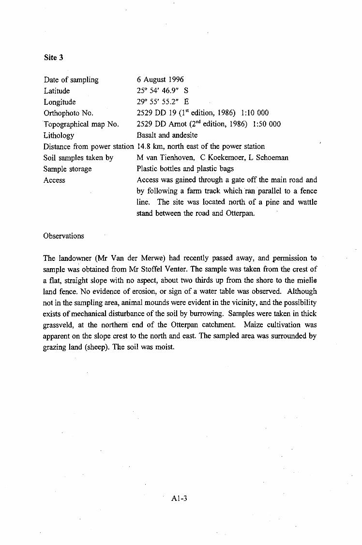
Site 3

Date of sampling

Latitude

Longitude

Orthophoto No.

Topographical map No.

Lithology

6 August 1996

25° 54' 46.9" s 29° 55' 55.2" E

2529 DD 19 (1st edition, 1986) 1: 10 000

2529 DD Arnot (2"d edition, 1986) 1 :50 000

Basalt and andesite

Distance from power station 14.8 km, north east of the power station

Soil samples taken by M van Tienhoven, C Koekemoer, L Schoeman

Sample storage Plastic bottles and plastic bags

Access

Observations

Access was gained through a gate off the main road and

by following a farm track which ran parallel to a fence

line. The site was located north of a pine and wattle

stand between the road and Otterpan.

The landowner (Mr Van der Merwe) had recently passed away, and permission to

sample was obtained from Mr Stoffel Venter. The sample was taken from the crest of

a flat, straight slope with no aspect, about two thirds up from the shore to the mielie

land fence. No evidence of erosion, or sign of a water table was observed. Although

not in the sampling area, animal mounds were evident in the vicinity, and the possibility

exists of mechanical disturbance of the soil by burrowing. Samples were taken in thick

grassveld, at the northern end of the Otterpan catchment. Maize cultivation was

apparent on the slope crest to the north and east. The sampled area was surrounded by

grazing land (sheep). Tbe soil was moist.

Al-3

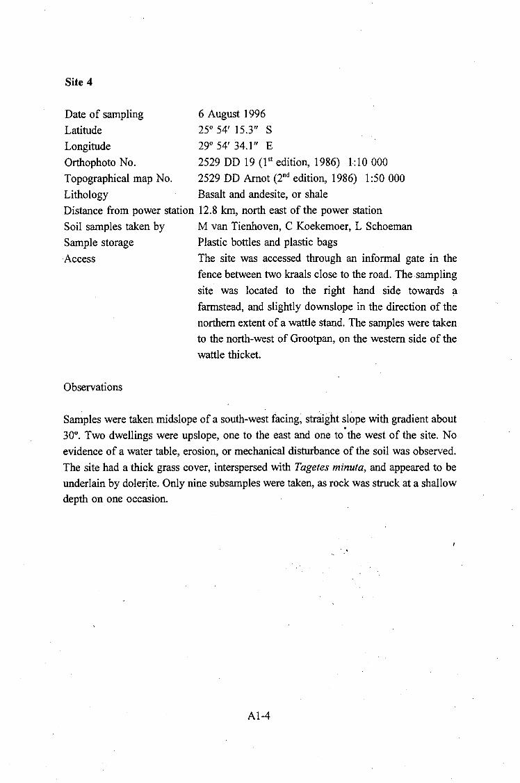
Site 4

Date of sampling

Latitude

Longitude

Orthophoto No.

Topographical map No.

Lithology

6 August 1996

25° 54' 15.3" s 29° 54' 34.1" E

2529 DD 19 (1st edition, 1986) l: 10 000

2529 DD Arnot (2nd edition, 1986) 1 :50 000

Basalt and andesite, or shale

Distance from power station 12.8 km, north east of the power station

Soil samples taken by M van Tienhoven, C Koekemoer, L Schoeman

Sample storage Plastic bottles and plastic bags

Access

Observations

The site was accessed through an informal gate in the

fence between two kraals close to the road. The sampling

site was located to the right hand side towards a

farmstead, and slightly downslope in the direction of the

northern extent of a wattle stand. The samples were taken

to the north-west of Grootpan, on the western side of the

wattle thicket.

Samples were taken midslope of a south-west facing~ str'1ight slope with gradient about

30°. Two dwellings were upslope, one to the east and one to· the west of the site. No

evidence of a water table, erosion, or mechanical disturbance of the soil was observed.

The site had a thick grass cover, interspersed with Tagetes minuta, and appeared to be

underlain by doler~te. Only nine subsamples were taken, as rock was struck at a shallow

depth on one occasion.

Al-4

Site 5

Date of sampling

Latitude

Longitude

Orthophoto No.

Topographical map No.

Lithology

6 August 1996

25° 53' 23.1" s 29° 52' 47.7" E

2529 DD 13 (1st edition, 1986) 1: 10 000

2529 DD Arnot (2"d edition, 1986) 1 :50 000

Shale

Distance from power station 10. 7 km, east-south east of the power station

Soil samples taken by M van Tienhoven, C Koekemoer, L Schoeman

Sample storage Plastic bottles and plastic bags

Access

Observations

Permission to sample was obtained at the farmstead (Mr

Combrink) situated north east of the Klippan. Access to

the site was gained through large double gates, about 1 km to the south of the farmstead. A farm track leads

south but we left the track and headed north towards the

farmstead.

The soil sampling site was located about three quarters upslope between the water's

edge and the road, to the south of a large, tree-covered rock outcrop. A dolerite outcrop

extended around one fifth of the pan. The rest of the pan was surrounded by grazing

land, with maize crops near the north-western and south-eastern shore. Marshy areas

were present to the north and south of the pan. The sampling site was sloped at about

35°, convex, with a western aspect and covered by grassveld. The soil was clayey and

moist, with some evidence of mottles. No evidence of a water table, erosion or

mechanical disturbance was observed.

Al-5

Site 6

Date of sampling

Latitude

Longitude

Orthophoto No.

Topographical map No.

Lithology

6 August 1996

25° 56' 08.5" s 29° 47' 53.3" E

2529 DD 16 & 17 (!51 editions, 1986) 1 :10 000

2529 DD Arnot (2"d edition, 1986) 1 :50 000

Shale

Distance from power station 1.3 km, north east of the power station

Soil samples taken by M van Tienhoven, H Dodds

Sample storage Plastic bottles and plastic bags

Access

Observations

A dirt road ran from the tar road to the east of the power

station, and could be followed to the railway line, where

access to the site was gained by climbing over a collapsed

fence.

The site was situated in a wedge of land hemmed in by the railway line, the road and

ESKOM land which possibly served as a coal stockpile area in the past. Maize fields

and a stand of oak trees were directly upslope of the site, and grazing land was

immediately downslope. Samples were taken from the upper midslope position, on a

straight, roughly 25° slope covered by grassveld and subject to cattle grazing. No

evidence of erosion or sign of a water table was observed. The openings of

subterranean termite tunnels were abundant, and mechanical disturbance of the soil by

these animals was a possibility. The soil was dry and the surface was quite sandy and

stony.

Al-6

Site 7

Date of sampling

Latitude

Longitude

Orthophoto No.

Topographical map No.

Lithology

7 August 1996

25° 54' 30.6" s 29° 51' 34.5" E

2529 DD 18 (151 edition, 1986) 1:10 000

2529 DD Arnot (2"d edition, 1986) 1 :50 000

Shale

Distance from power station 8.1 km, south east of the power station

Soil samples taken by M van Tienhoven, C Koekemoer, L Schoeman

Sample storage Plastic bottles and plastic bags

Access

Observations

· The site was situated on mine land. A gate (signposted

'Refuge Bay 9') led directly onto a dirt track which was

navigable by car, provided a sharp lookout was kept for

fugitive barbed wire.

Samples were taken from a site on the eastern shore of the pan, with a wattle stand

about 100 metres to the south-and a large wattle thicket about 300 metres to the north.

The pan was surrounded by grazing land (horses) with maize lands on the southern

crest, and there was evidence of excavation on the eastern shore (failed dam?), about

half way between the road and the water. A dolerite outcropping occured to the north,

and a stand of blue gum trees to the north east. The site was situated on a slightly

concave, roughly 20° slope with a north-west aspect, and samples were taken from the

upper midslope. The soil was sandy and was covered by thick, heavily grazed grassveld

with sparsely dispersed khakibos (Tagetes minuta). No evidence of erosion or sign of

a watertable was observed, but small termite mounds and an old road were apparent in

the vicinity, and could indicate potential mechanical disturbance of the soil.

Al-7

Site 8

Date of sampling

Latitude

Longitude

Orthophoto No.

Topographical map No.

Lithology

7 August 1996

25° 58' 35.9" s 29° 55' 38.0" E

2529 DD 24 (!51 edition, 1986) 1: 10 000

2529 DD Arnot (2"d edition, 1986) 1 :50 000

Shale

Distance from power station 14.4 km, east-south east of the power station

Soil samples taken by M van Tienhoven, C Koekemoer, L Schoeman

Sample storage Plastic bottles and plastic bags

Access

Observations

The site was situated on mine land, and could be entered

through a gate leading directly off the road and signposted

'WJ'.

A stand of wattle trees lay to the south west of the pan, while maize fields were present

to the north, east and south and were interspersed with grazing veld. Soil samples were

taken on the north-eastern side of the pan, about 30 metres from a large, single wattle

tree. An outcrop of possibly sandstone emerged close to the pan. The sampling site was

situated on the upper midslope to crest of a straight, roughly 10° slope with a south east

aspect. The soil was moist and sandy and had a good grass cover dominated by

Eragrostis. Some animal burrows and slight depressions were evident in the vicinity of

the site, and there was no evidence of erosion or sign of a water table. Only 9 subsoil

subsamples were taken, as rock was repeatedly struck in one of the subsample sites.

Al-8

Site 9

Date of sampling

Latitude

Longitude

Orthophoto No.

Topographical map No.

Lithology

6 August 1996

25° 57' 11.1" s 29° 54' 36.9" E

2529 DD 24 (!51 edition, 1986) 1:10 000

2529 DD Arnot (2"d edition, 1986) 1 :50 000

Dolerite

Distance from power station 12.6 km, east of the power station

Soil samples taken by M van Tienhoven, H Dodds, C Koekemoer, L Schoeman

Sample storage Plastic bottles and plastic bags

Access

Observations

The site was situated on mining land. Access was gained

through a farm gate marked 'W8' located opposite

Klipfontein farm.

The sampling site was roughly in line with the western post of the gate, about 50 metres

from the road, and was covered by grazed grassveld. On entry through the gate there

was a disused concrete threshing floor 10 m in diameter located on the right hand side.

Samples were taken from the midslope of a approximately 15° slope with a north east

aspect. There was no evidence of erosion or signs of a water table, although patches

of damp, dark soil were observed. Termite or dung beetle burrows were also observed.

Surface rock outcrops were evident.

Al-9

Site 10

Date of sampling

Latitude

Longitude

Orthophoto No.

Topographical map No.

Lithology

7 August 1996

25° 58' 29.8" s 29° 51' 55.3" E

2529 DD 23 (1st edition, 1986) 1: 10 000

2529 DD Arnot (2nd edition, 1986) 1 :50 000

Dolerite

Distance from power station 8.3 km, east-south east of the power station

Soil samples taken by M van Tienhoven, H Dodds, C Koekemoer, L Schoeman

Sample storage Plastic bottles and plastic bags

Access

Observations

The site was accessed through a driveway with large,

ornate, concrete posts on either side. A side gate led into

the paddock directly from the driveway. The nearby

homestead "Leeupan" is distinguished by two large palm

trees. The house was close to the road.

The sampling site lay 40m to the north-east of a survey beacon, roughly 100 m to the

north of the farmstead, and was covered by thick, waist-high grassland with some

Themeda. Some evidence of grazing was observed, but this was neither intensive nor

recent. The site was situated on the crest of a very slightly concave slope of about 5 to

10° and with a north aspect. There was no evidence of erosion, mechanical disturbance

or sign of a water table. The soil was a moist, heavy, black clay, and contained very

dark to black concretions of about 3 mm diameter.

Al-10

Site 11

Date of sampling

Latitude

Longitude

Orthophoto No.

Topographical map No.

Lithology

7 August 1996

25° 59' 02.4" s 29° 47' 03.5" E

2529 DD 21 (151 edition, 1986) 1:10 000

2529 DD Arnot (2"d edition, 1986) 1 :50 000

Shale

Distance from power station 4.5 km, south west of the power station.

Soil samples taken by M van Tienhoven, C Koekemoer, L Schoeman

Sample storage Plastic bottles and plastic bags

Access

Observations

The site was accessible by a service road for the power

line which runs through the area. Access to this route is

from the public road but through a series of locked gates

the keys to which were supplied by Mr Koekemoer.

The sampling site lay directly to the south of the nearby pan. with an avenue of oak

trees and powerlines south of the site. The soil was moist and sandy and was well

covered by grassveld, predominantly "kweekgras", which appeared to be grazed b,y cattle. The site was situated in the upper midslope of a slightly concave, south facing

slope of gradient about 10°. There was no evidence of erosion, mechanical disturbance

or sign of a water table.

Al-11

Site 12

Date of sampling

Latitude

Longitude

Orthophoto No.

Topographical map No.

Lithology

8 August 1996

25° 55' 55.2" s 29° 50' 28.0" E

2529 DD 17 (1st edition, 1986) 1: 10 000

2529 DD Arnot (2"d edition, 1986) 1 :50 000

Shale

Distance from power station 5.5 km, east-north east of the power station

Soil samples taken by M van Tienhoven, H Dodds

Sample storage Plastic bottles and plastic bags

Access

Observations

The site was situated on mine land and could be accessed

using a dirt road which ran to the east of Rietkuil, and

then turning off onto a farm road. During the week of

sampling, minor detours were encountered along this

route, possibly because of the movement of test drill rigs

which were shifted from site to site. It is possible that

further modification of these roads may occur in the

future.

The site was covered by grassveld and subject to sheep and cattle grazing. Soil was

~ampled from the midslope position of a straight,. south-west facing slope with a

gradient of about 15°, north of a windmill. No evidence of erosion nor sign of a water

table was observed. Animal burrows and tracks were evident.

Al-12

Site 13

Date of sampling

Latitude

Longitude

Orthophoto No.

Topographical map No.

Lithology

8 August 1996

25° 58' 44.4" s 29° 49' 56.9" E

2529 DD 22 (!81 edition, 1986) 1: 10 000

2529 DD Arnot (2"d edition, 1986) I :50 000

Shale

Distance from power station 5.8 km, south-west of the power station

Soil samples taken by M van Tienhoven, H Dodds

Sample storage

Access

Observations

Plastic bottles and plastic bags

The site was accessed by driving along the dirt road

which ran parellel to the ash dam, turning to the east at a

large, fenced off area which marked the junction of

underground water mains and is termed "Picadilly circus".

Head into the veld to the south of a fence post which

marks the beginning of an east-running farm fence. It

was possible to drive a car over the flat terrain. The land

is privately owned, and Mr Koekemoer obtained

permission for sampling.

The site was situated on lightly-grazed grassveld on the north-eastern side of the nearby

pan, and immediately upslope of a broad band of low-growing bush (possibly Stoebe

vulgaris) which extended downslope towards the shore. Extensive khakibos

establishment was also evident on the eastern side of the pan. A rural settlement was

situated to the north-north east, behind a wattle thicket. Soil was sampled from the

upper midslope to crest of a slightly convex, south-east facing slope with a gradient of

roughly 10°. No sign of erosion or a water table was evident. The soil was moist.

Animal burrows and cattle tracks were observed.

Al-13

Site 14

Date of sampling

Latitude

Longitude

Orthophoto No.

Topographical map No.

Lithology

8 August 1996

25° 59' 36.9" s 29° 58' 10.l" E

2529 DD 25 (1st edition, 1986) 1: 10 000

2529 DD Arnot (2"d edition, 1986) 1 :50 000

Quartzite and shale, or tillite and shale

Distance from power station 18.8 km, east-south east of the power station

Soil samples taken by M van J'ienhoven, H Dodds

Sample storage

Access

Observations

Plastic bottles and plastic bags

The landowner, Mr Combrink, was approached for

permission to sample on his land. The farmstead

"Goedehoop" was about 1 km from the main dirt road, on

the western side of the farm access road. The site itself

was further to the west, in a paddock which lay directly

next to the main dirt roa:d. A road beacon labelled

"l/D248" lay parallel to the sampling site. The site was

located downslope of the road and access required

climbing through the fence.

The site was covered by well-established grassveld, with a very diverse species

composition and very lightly grazed by antelope. The last time the soil had been

ploughed was about 50 years ago. Animal burrows and tracks were evident, but were

very sparse. Soil was collected from midslope of a straight, north facing slope with a

gradient of about 10°. There was no evidence of erosion or a water table.

Al-14

Site 15

Date of sampling

Latitude

Longitude

Orthophoto No.

Topographical map No.

Lithology

9 August 1996

25° 57' 20. 7" s 29° 47' 05.2" E

2529 DD 21 (!51 edition, 1986) 1:10 000

2529 DD Arnot (2"d edition, 1986) 1 :50 000

Shale

Distance from power station 1.0 km, south-south west of the power station

Soil samples taken by M van Tienhoven, H Dodds

Sample storage Plastic bottles and plastic bags

Access

Observations

A public tar road runs south of the power station. Large

white brick walls flanked an access road which runs north

towards the power station. The turnoff to the access road

was also marked by a stand of pine trees. The access

road forked, and the right hand fork was followed for

about 50 metres, until immediately before a farmstead

surrounded by a large, high security fence. The site lay

about 40 meters to the south of the road and could be

entered by climbing over the fence.

The site was located in a tract of natural veld which was not extensively grazed, and

which was wedged in between the farmstead and a maize field to the east and south

east, and a housing development to the north, directly upslope. Soil samples were taken

midslope of a straight, south-west facing slope with a gradient of about 15°. No

evidence of erosion or sign of a water table was observed. A few animal burrows were

noted.

Al-15

APPENDIX 2 - ANALYTICAL METHODS

1. Geographical Positioning System . . . . . . . . . . . . . . . . . . . . . . . . . . . . A2-1

2. Sample preparation . . . . . . . . . . . . . . . . . . . . . . . . . . . . . . . . . . . . . A2-1

3. Determination of pH in water, KCl and K2S04 • • • • • . • • • • • • . • • • • • A2-1

4. Determination of acid neutralising capacity . . . . . . . . . . . . . . . . . . . . . A2-3

5. Determination of exchangeable cations . . . . . . . . . . . . . . . . . . . . . . . . A2-4

6. Determination of exchangeable acidity .... : . . . . . . . . . . . . . . . . . . . A2.;.4

7. Determination of exchangeable calcium and magnesium . . . . . . . . . . . . A2-4

8. Preparation of saturated soil paste extracts . . . . . . . . . . . . . . . . . . . . . . A2-5

9. Determination of soluble ions by ion chromatography . . . . . . . . . . . . . . A2-5

10. Determination of organic carbon . . . . . . . . . . . . . . . . . . . . . . . . . . . A2-6

11. Determination of soil moisture content . . . . . . . . . . . . . . . . . . . . . . . A2-7

12. Particle size analysis ... ·. . . . . . . . . . . . . . . . . . . . . . . . . . . . . . . . . A2-7

13. Determination of extractable iron, aluminium and manganese: dithionite-

citrate-bicarbonate. . . . . . . . . . . . . . . . . . . . . . . . . . . . . . . . . . . . . A2-8

14. Determination of mineralogical composition of sand, silt and clay fractions A2-9

15. Sample preparation for XRF spectrometry . . . . . . . . . . . . . . . . . .. . . . A2-9

16. Routine analysis of trace and major elements by wavelength dispersive X-

ray fluorescence spectrometry . . . . . . . . . . . . . . . . . . . . . . . . . . . . . A2-10

16.1. Major elements . . . . . . . . . . . . . . . . . . . . . . . . . . . . . . . . . . A2-10

16.2. Trace elements . . . . . . . . . . . . . . . . . . . . . . . . . . . . . . . . . . A2-11

APPENDIX 2 - ANALYTICAL METHODS

Many of the analytical techniques described in the following section are standard techniques

which are readily available in standard texts or from the scientific literature. However, if valid

comparisons are to be made between the data collected in this study and data to be collected

in the future, the methods employed must be repeatable. Thus, wherever possible, details of

each method have been noted.

1. Geographical Positioning System

A GARMIN GPS 45 navigator was used to locate the position of the sampling sites. The

Geographical Positioning System (GPS) is operated by the government of the United States

of America, which is solely responsible for its accuracy and maintenance. The system is

currently under development and is subject to changes which could affect the accuracy and

performance of all GPS equipment. Thus, supplementary information from local maps and

site-specific features were noted to ensure that each soil sampling site could be relocated in

the future. .

The GARMIN GPS 45 features a MultiTrac8™ receiver which tracks and uses up to eight

satellites simultaneously. Position accuracy ranges from 5 to 15 meters. The map datum field

used as the default setting is the World Geodetic System 1984 (GARMIN GPS 45 Instruction

Manual).

2. Sample preparation

Each soil sample was poured out into a clean, dry soil tray and left to air dry indoors for three

to four days. Once dry the soil was ground to pass through a 2 mm soil sieve, then stored in

plastic jars with airtight screw-on lids. Unless otherwise stated airdried, sieved soil was used

in all analyses. Reference samples are kept by both the CSIR (Nelspruit) and the Department of Geological Sciences, University of Cape Town, Cape Town.

3. Determination of pH in water, KCI and K2S04

The pH in distilled water, 1 M KCl and 0.5 M K2S04 was determined for each soil according

to the method of McLean (1982). A 1 :2.5 ratio of soil:solution was used. The soils were

shaken for 10 minutes on a reciprocal shaker and left to stand for 30 minutes prior to pH measurement. The pH was measured with a glass electrode paired with a calomel (Hg-Hg2Cl)

A2-1

-- - __ _J

reference electrode, using a Crisan micropH 2001 pH meter. The pH meter was calibrated

daily with buffers pH 4.01 and pH 7.00. The electrode was lowered into the solution until the

tip was just above the settled soil layer. The pH was recorded once the digital reading was

stable for at least I 0 seconds. In the case of pH in distilled water, the electrode was immersed

for a minute before the reading was taken.

Instrument precision was tested by 3 non-consecutive measurements of the same extract. The

details for extracts of samples ST and 13S are shown in Table A2.1 - for pH in water, KCl

and K2S04•

Table A2.1

Sample

ST

13S

x

Precision of pH measurements for extracts of samples ST and 13S -

determined by 3 non-consecutive measurements of the extract (n=3). Results

are shown for pH in water, KCl and K2S04•

pH (water) pH (KCl) pH(K2S04)

s RSD1 x s RSD x s RSD

S.47 0.006 0.1% 4.30 0.006 0.1% 4.7S 0.006 0.1%

S.49 0.036 0.7% 4.26 0.006 0.1% 4.82 0 0%

RSD = relative standard deviation

In general there was far more variation in the measurements of pH in water than for those

made in either KCI or K2S04•

The repeatability of the extractions was also tested by perfomiing six repeats of each

extraction on samples 6T and 13T. Results are presented in Table A2.2.

Table A2.2

Sample

6T

13T

Repeatability of extractions in water, KCl and K2S04 performed for samples 6T and 13T (n=6).

pH (water) pH (KCl) pH (K2S04)

x s RSD 1 x s RSD x s RSD

S.23 0.016 0.3% 4.11 0.021 O.S% 4.60 0.027 0.6%

S.79 0.037 0.6% 4.43 0.014 0.3% 4.8S 0.037 0.8%

RSD = relative standard deviation

-Note that it is mathematically incorrect to average pH values (since pH = - log [H+]). Yet

converting the pH values of a few samples to the Hi- concentrations, finding the mean and

converting back to pH, revealed no difference in the pH averages. For the sake of efficiency

all subsequent pH values were averaged without converting to [H'J

A2-2

4. Determination of acid neutralising capacity

The acid neutralising capacity (ANC) of soil estimates the extent to which acidifying activities,

such as cropping or atmospheric deposition, are held in check before the soil is seriously

degraded. Thus, ANC provides an indication of the resilience or buffering capacity of the ecosystem to acid inputs.

Two methods of determining ANC are generally employed - both approaches are time­

consuming and costly. The method of van Breemen et al. (1983) requires a full assay of the

total basicity present while the second method involves a serial titration and equilibration with

strong acids (Natscher and Schwertmann, 1991, cited in du Toit, 1993a). A more efficient

means of determining ANC was developed by B du Toit (1993) and du Toit and Fey (1994),

whereby the same chemical principles used to determine the base neutralising capacity of soils

(BNC) or lime requirement were adapted to the determination of ANC.

A buffer mixture of 0.01 moles HOAc, 0.001 moles KOAc and 0.1 moles (11. lg) of CaCl2

was made up to 1 liter and adjusted to pH 3.5. Five mL of soil were mixed with 15 mL of

the buffer solution and the suspension shaken for 15 minutes. After shaking, the suspension

was allowed to settle for 15 minutes before the pH of the supernatant solution was recorded.

ANC was calculated as follows:

ANC (cmolc-L-1) = 9.624 (pH) - 34.13

where an ANC of 1 cmolc.L·1 is equivalent to 1 t CaC03.ha·1.20 cm.

Du Toit {1993a) found an excellent correlation (r2 = 0.96) between the pH of the soil-buffer

solution and soil ANC derived by the method of Natscher and Schwertmann (1991).

The ANC was determined on duplicates for each soil sample in the present study but for some

samples the determination was repeated 3 or 4 times to test precision. The results are reported in Table A2.3.

Table A2.3 Repeatability of ANC determinations

Sample n Average (x) Sample standard Relative standard ( cmolc.L ·1

) deviation ( s) deviation

IT 4 4.70 0.17 3.5% 6T 4 2.51 0.05 1.9% 7S 3 3.18 0.15 4.6%

A2-3

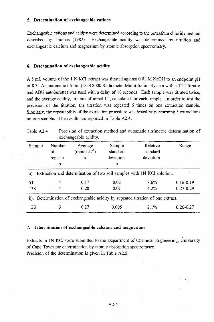
5. Determination of exchangeable cations

Exchangeable cations and acidity were determined according to the potassium chloride method

described by Thomas (1982). Exchangeable acidity was determined by titration and

exchangeable calcium and magnesium by atomic absorption spectrometry.

6. Determination of exchangeable acidity

A 5 mL volume of the I N KCI extract was titrated against 0.01 M NaOH to an endpoint pH

of 8.3. An automatic titrator (DTS 8000 Radiometer Multititration System with a TTT titrator

and ABU autoburette) was used with a delay of IO seconds. Each sample was titrated twice,

and the average acidity, in units of mmol.L-1, calculated for each sample. In order to test the

precision of the titration, the titration was repeated 6 times on one . extraction sample.

Similarly, the repeatability of the extraction procedure was tested by performing 5 extractions

on one sample. The results are reported in Table A2.4.

Table A2.4 Precision of extraction method and automatic titrimetric determination of exchangeable acidity.

Sample Number Average Sample Relative Range of (mmolc.L-1

) standard standard repeats x deviation deviation

n ·s

a). Extraction and determination of two soil samples with IN KCl solution.

ST 4 0.17 0.02 8.6% 0.16-0.19 13S 4 0.28 0.01 4.2% 0.27-0.29

b ). Determination of exchangeable acidity by repeated titration of one extract.

13S 6 0.27 0.005 2.1% 0.26-0.27

7. Determination of exchangeable calcium and magnesium

. Extracts in IN KCI were submitted to the Department of Chemical Engineering, University

of Cape Town for determination by atomic absorption spectrometry.

Precision of the determination is given in Table A2.5.

A2-4

Table A2.S Repeatability of extraction method and determination of calcium and magnesium by atomic absorption spectrometry.

Sample n Sample mean (x) Sample standard Relative standard (mg.kg-1 soil) deviation ( s) deviation

Calcium ST s 276.0 S.7 2.1% 13S s 141.4 10.S 7.5%

Magnesium ST s 220.2 2.S 1.2% 13S s 112.9 S.S 4.9%

Cation exchange capacity (CEC) is normally expressed as mmoles charge per kg of soil. It

is a measure of the quantity of readily exchangeable cations neutralising the negative charge

in the soil. CEC is estimated by taking the sum of exchangeable cations present in the

leachate after exposure to a saturating salt solution. - termed the summation method as

(Rhoades 1982b ). The effective cation exchange capacity (ECEC) is calculated from the

concentrations of Ca2+, Mg2

+ and ~ cations extracted by 1 N KCI.

8. Preparation of saturated soil paste extracts

Preparation of the saturated paste extracts was performed by the Agricultural Research Council

in Nelspruit according to the procedure outlined by Rhoades (1982a). Soil pH of the fresh

extract was not recorded. Once extracted the solution was refrigerated and frozen. During

transportation from Nelspruit to Cape Town the extracts were kept as cool as possible but

considerable thawing nevertheless occurred.

The saturated paste extracts were filtered through a 0.4S µm filter and the electrical

conductivity of each solution was determined.

The concentrations of soluble salts in the saturated paste extracts were determined by ion

chromatography. Dilution of the extracts was often necessary to prevent damage to the ion

chromatography column. Extracts were diluted to achieve an electrical conductivity below

100 µS.cm- 1•

9. Determination of soluble ions by ion chromatography

All soil solutions were filtered through a 0.4S µm filter and a Dionex On-Guard-P cartridge for the removal of organic colloids.

A2-S

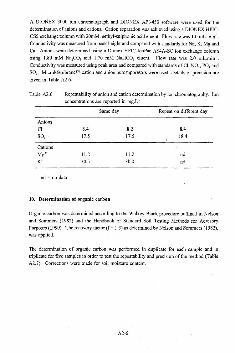
A DIONEX 3000 ion chromatograph and DIONEX API-450 software were used for the

determination of anions and cations. Cation separation was achieved using a DI ONEX HPIC­

CS5 exchange column with 20mM methyl-sulphonic acid eluent. Flow rate was 1.0 mL.min-1•

Conductivity was measured from peak height and compared with standards for Na, K, Mg and

Ca. Anions were determined using a Dionex HPIC-IonPac AS4A-SC ion exchange column

using 1.80 mM NazC03 and 1.70 mM NaHC03 eluent. Flow rate was 2.0 mL.min-1•

Conductivity was measured using peak area and compared with standards of Cl, N03, P04 and

S04• MicroMembrane™ cation and anion autosuppresors were used. Details of precision are

given in Table A2.6.

Table A2.6 Repeatability of anion and cation determination by ion chromatography. Ion

concentrations are reported in mg.L ·1

Cations Mg2+

K+

nd =no data

8.4

17.5

11.2

30.5

Same day

10. Determination of organic carbon

8.2

17.5

11.2

30.0

Repeat on different day

8.4

18.4

nd

nd

Organic. carbon was determined according to the Walkey-Black procedure outlined in Nelson

and Sommers (1982) and the Handbook of Standard Soil Testing Methods for Advisory

Purposes (1990). The recovery factor (f = 1.3) as determined by Nelson and Sommers (1982),

was applied.

The determination of organic carbon was performed in duplicate for each sample and in

triplicate for five samples in order to test the repeatability and precision of the method (Tao1e

A2.7). Corrections were made for soil moisture content.

A2-6

Table A2.7 Reproducibility of the Walkley-Black determination of organic carbon. Values given are% organic carbon (without soil moisture correction).

Sample n Sample mean Sample standard Relative standard Range (x) deviation ( s) deviation

IT 3 4.3 O. I 2.3 % 4.2-4.4 IS 4 2.3 0.4 I5.6% 1.9-2.6 SS 3 1.3 0.1 8.7% 1.2-1.4 9S 3 1.6 O.I 3.7%. 1.5-1.6 I2S 3 1.3 0 0%

11. Determination of soil moisture content

Exactly 30 g of airdried soil, sieved to pass through a 2 mm sieve, were weighed out into a

pre-weighed glass petri dish. The dishes were placed in an oven at 90 °C for 72 hours until

a constant mass (y) was achieved. T~e mass was determined immediately on removal from

the oven to reduce moisture uptake from the air by the soil. Percentage moisture content was

calculated as below:

% moisture content = (30 g air dry soil - y) x 100

30 g

Percentage moisture estimates are based on only one determination per sample.

12. Particle size analysis

The mass of the bulk soil sample was measured before sieving through a 2 mm soil sieve.

After sieving, the mass of the gravel fraction remaining in the sieve was measured and

reported as a fraction of the bulk soil.

The sand, silt and clay fractions of each soil were determined according to the standard

methods employed py the Institute for Tropical and Sub-tropical Crops (Agricultural Research

Council) in Nelspruit, Mpumalanga. The method is based on Stoke's Law which is well

outlined in basic soil texts such as Kohnke (1968).

Air dry soil, sieved to pass through a 2 mm sieve, was poured into a 250 mL glass beaker.

For fine-textured soils 50 g of material were used, whereas IOO g were used for sandy soils.

Approximately 200 mL of distilled water were added to the soil in the beaker together with

5 mL of IN sodium hexametaphosphate. The sodium hexametaphosphate acts to disperse the

A2-7

clay by removing or complexing polyvalent cations and replacing these with the monovalent

sodium cation (Kohnke, 1968). The mixture was left to equilibrate overnight.

The slurry was then decanted into a stainless steel mixing flask, rinsing the original beaker

thoroughly with distilled water to ensure that all the soil was transferred. The mixing flask

was then filled with distilled water to make a total volume of about 500 mL. Clay soils were

mixed for 15 minutes while sandy soils required only ten minutes. After mixing, the flask was

removed from the mixer, ensuring that any soil on the mixing shaft was rinsed into the flask.

The slurry was decanted into a standardised de Bouyoucos soil cyclinder and distilled water

added almost to the mark (1130 mL for 50 g of clay soils or 1205 mL mark for 100 g of

sandy soils). The soil hydrometer was placed into the cyclinder and allowed to settle before

the cylinder was filled completely to the appropriate mark. Two or three drops of pure amyl

alcohol were added to ensure that organic matter did not stick to the hydrometer and interfere

with its operation. The hydrometer was removed, the lid placed on the cylinder and the

cylinder inverted ten times to ensure good mixing. Once shaken the cyclinder was

immediately placed on a firm surface, the lid removed and the hydrometer gently immersed

in the solution. Reading A was taken exactly 4 minutes after shaking (sand fraction). The

cylinder was left undisturbed for a further two hours before taking reading B (clay fraction).

A ZEAL hydrometer was used for all of the determinations. The particle size fractions were

calculated as fol1ows:

% sand

% clay

% silt

= 100 - (Reading A/mass of soil used)

= Reading B/mass of soil used

= 100 - (%sand+% clay)

where the fractions are defined as sand: 2.00 - 0.002 mm silt: 0.02 - 0.002 mm

clay: < 0.002 mm

Only one determination was performed per sample.

13. Determination of extractable iron, aluminium and manganese: dithionite-citrate­bicarbonate.

Free· iron and aluminium oxides in the soils were determined by the Institute for Soil, Climate

and Water according to the method prescribed by Jackson, Lim and Zelazny (1986) and the

Handbook of Standard Soil Testing Methods for Advisory Purposes (1990). Once the free

iron, aluminium and manganese hade been extracted, their concentrations were determined by

atomic absorption spectrometer.,.

A2-8

14. Determination of mineralogical composition of sand, silt and clay fractions

Mineral identification in the sand, silt and clay fractions was performed by X-ray diffraction by the Institute for Soil, Climate and Water.

15. Sample preparation for XRF spectrometry

Powder briquettes and fusion discs for analysis by X-ray fluorescence spectrometrywere

prepared according to the standard method employed by the Department of Geological Sciences, University of Cape Town.

A 50 g mass of each soil was milled in a Sieb swing mill with a carbon steel vessel for 2

minutes at the fast setting. Plastic gloves and a clean wooden spatula were used to transfer

the milled soil to a plastic bag which was then sealed. The Sieb mill was cleaned between

samples by milling with quartz for one minute. The milled quartz was discarded and the mill

cleaned with compressed air under an extraction fan to reduce dust contamination. The milled

was then washed under tap water, rinsed with distilled water, dried off and finally rinsed and dried with acetone.

Preparation of powder briquettes for trace element determination:

Six grams of the milled soil were mixed with 6 drops of 4 % Mowial using an agate pestle

and mortar. Once mixed the powder was pressed into a briquette using boric acid as the binder.

Preparation of Norrish fusion discs for major element determination:

The method of Norrish and Hutton (1969) was employed for the preparation of fusion discs.

Additional details of the preparation of glass discs and a discussion of the potential sampling

errors and contamination problems are given by Claisse and Willis (1995).

A2-9

16. Routine analysis of trace and major elements by wavelength dispersive X-ray fluorescence spectrometry

The following information is taken directly from Willis (1996) and provides details of the

XRF instrument parameters and calculations performed in estimating major and trace element

data,

16.1. Major elements

Nine major elements, Fe, Mn, Ti, Ca, K, P, Si, Al and Mg (with Ni and Cr when Ni and Cr

concentrations exceed -2000 ppm or 0.2 %) are determined using fusion disks prepared

according to the method of Norrish·and Hutton (1969). The disks are analyzed on a Philips

PW1480 wavelength dispersive XRF spectrometer with a dual target Mo/Sc x-ray tube. Fe,

Mn and Ti are measured with the tube at 100 kV, 25 mA. The other elements are determined

with the tube at 40 kV, 65 mA. Peak only measurements are made on the elements Fe through

Mg. Sodium is determined using powder briquettes, the x-ray tube at 40 kV, 65 mA, and with

backgrounds measured at -2.00 and +2.00°28 from the peak position. Analytical conditions

are given in Table A2.8.

Fusion disks made up with 100% Johnson Matthey Specpure Si02 are used as blanks for all

elements except Si. Fusion disks made up from mixtures of Johnson Matthey Specpure Fe20 3

and CaC03 are used as blanks for Si. Intensity data are collected using the Philips X40

software. Matrix corrections are made on the elements Fe _through Mg using the de Jongh

model in the X40 software. Theoretical alpha coefficients used in the de Jongh model for all

other elements on the analyte element are calculated using the Philips on-line ALPHAS

programme. N<1i0 is not included in the matrix corrections in de Jongh model, and no matrix

corrections are made to the sodium intensities.

Table A2.8. Analytical conditions for determination of major elements using a Philips

PW1480 WDXRF spectrometer.

Element/ Crystal Detector

PHS Counting Concentration No. of

line Collimator

LWL UPL time (s) range* RMS

standards

FeKa F LiF(220) FL 16 70 150 0 - 17 0.118 14

MnKa F LiF(220) FL 15 70 150 0 - 0.22 0.005 14

Ti Ka F LiF(200) FL 28 70 150 0 - 2.75 0.020 14

Ca Ka F LiF(200) FL 36 70 20 0 - 12.5 0.037 14

KKa F LiF(200) FL 36 70 50 0 - 15.5 0.057 14

PKa c GE(! I I) FL 25 75 100 0 - 0.36 0.008 14

Si Ka c PE(002) FL 32 74 100 0 - 100 0.408 14

Al Ka c PE(002) FL 25 75 80 0 - 17.5 0.136 14

· MgKa F PX-I FL 30 74 150 0 - 46 0.095 14

NaKa F PX-I FL 30 78 200 0 - 9 0.189 15

* all concentrations expressed as wt% oxide

16.2. Trace elements

Trace elements were determined on powder briquettes in a series of analytical runs using a

number of different x-ray tubes. Analytical conditions are listed in Tables A2.9 and A2.10.

The RhKa Compton or the MoKa Compton peak is used to determine the mass absorption

coefficients of the specimens at the RhKaC wavelength or the MoKaC wavelength, and the

Compton peak mass absorption coefficient values are used to correct for absorption effects on

the Mo, Nb, Zr, Y, Sr, U, Rb, Th, Pb, Br, Se, Bi, As, W, Zn, Cu and Ni analyte wavelengths.

Primary and secondary mass absorption coefficients for the Co, Mn, Cr, V, La, Ce, Nd, Ba,

Sc, S and F analyte wavelengths are calculated from major ,element compositions using the

tables of Heinrich (1986). Mass absorption coefficient corrections are made to the net peak

intensities, (gross peak intensities corrected for dead time losses, background and sp(;!ctral

overlap), to correct for absorption differences between standards and specimens. No

corrections are made for enhancement, which could be small but significant(<~?% relative)

for the elements Cr, V, Ba and Sc in certain specimens, depending on their concentrations of Fe, Mn and Ti.

Measured intensity data are processed through the computer program TRACE to correct gross

peak intensities for background and spectral overlap and to make mass absorption coefficient

corrections according to the methods outlined in Duncan et al. (1984). First order calibration

lines with zero intercept are calculated using six or more international rock standard reference

materials (SRMs) for each element. The one standard deviation (1 cr) error due to counting

statistics and the lower limit of detection is calculated for each element in each specimen.

A2-11

Table A2.9 X-ray tubes and tube and x-ray path settings for the deterniination of trace

elements using a Philips PWl 480 WDXRF spectrometer.

X-ray tube Element/line X-ray path

Target kV - mA

MoKaC Mo/Sc 90 30 Vacuum

Mo Ka Rh 80 35 Vacuum

Nb Ka Rh 80 35 Vacuum

Zr Ka Rh 80 35 Vacuum

YKa Rh 80 35 Vacuum

Sr Ka Rh 80 35 Vacuum

ULa 1 Rh 80 35 Vacuum

Rb Ka Rh 80 35 Vacuum

ThLa1 Rh 80 35 Vacuum

PbL~ 1 Rh 80 35 Vacuum

Zn Ka Au 60 45 Vacuum

Cu Ka Au 60 45 Vacuum

NiKa Au 60 45 Vacuum

Co Ka Au 50 55 Vacuum

MnKa Au 50 55 Vacuum

Cr Ka Au 50 55 Vacuum

VKa Au 50 55 Vacuum

SKa Mo/Sc 40 65 Vacuum

FKa Mo/Sc 40 70 Vacuum

A2-12

Table A2.IO Instrumental conditions for determination of trace elements using a Philips PW1480 WDXRF spectrometer.

Element Collimator ' Crystal Detector PHS Counting Concentration /line LWL UPL time (s) range*

MoKaC F LiF(220) SC 32 74 200

Mo Ka F LiF(200) SC 30 74 200 0 - 280

Nb Ka F LiF(200) SC 30 74 200 0 - 268

Zr Ka F LiF(200) SC 30 74 200 0 - 1210

YKa F LiF(200) SC 30 74 200 0 - 143

Sr Ka F LiF(200) SC 30 74 ' 200 0 - 440

ULa1 F LiF(200) SC 30 74 200 0 - 15

Rb Ka F LiF(200) SC 30 74 200 0 - 530

ThLa1 F LiF(200) SC 30 74 200 0 - 51

PbL~ 1 F LiF(200) SC 30 74 200 0 - 40

ZnKa F LiF(220) FS 20 80 200 0 - 235

CuKa F LiF(220) FS 20 80 200 0 - 227

NiKa F LiF(220) FS 20 80 200 0 - 630

Co Ka F LiF(220) FL 15 75 200 0 - 116

MnKa F LiF(220) FL 15 75 200 0 - 1700

CrKa F LiF(220) FL 15 75 200 0 - 465

VKa F LiF(220) FL 13 67 200 0 - 640

SKa c Ge(l 11) FL 32 72 100

* all concentrations expressed as part per million (ppm or mg.kg- 1)

A2-13

l ~ .

'---------------------------------------- -

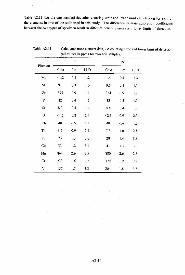
Table A2. l l lists the one standard deviation counting error and lower limit of detection for each of

the elements in two of the soils used in this study. The difference in mass absorption coefficients

between the two types of specimen result in different counting errors and lower limits of detection.

Table A2.l l Calculated trace element data, l cr counting error and lower limit of detection

(all values in ppm) for two soil samples.

IT IS Element

Cale I cr LLD Cale I cr LLD

Mo <1.2 0.4 1.2 1.4 0.4 1.3

Nb 9.3 0.4 1.0 9.5 0.4 1.1

Zr 395 0.9 1.1 364 0.9 IJ

y 12 0.4 1.2 13 0.5 1.3

Sr 8.0 0.4 1.2 4.8 0.4 1.2

u <1.2 0.8 2.4 <2.3 0.9 2.3

Rb 40 0.5 1.3 40 0.6 1.3

Th 6.2 0.9 2.7 7.3 1.0 2.8

Pb 23 1.3 3.6 28 1.4 3.8

Co 33 1.2 3.1 41 1.3 3.3

Mn 864 2.6 2.5 880 2.6 2.6

Cr 233 1.6 2.7 320 1.9 2.9

v 157 1.7 3.3 204 1.8 3.5

A2-14

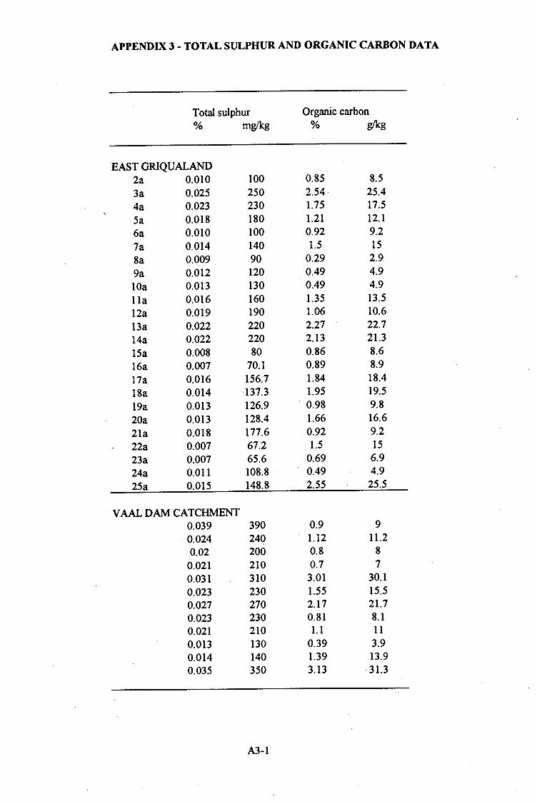
APPENDIX 3-TOTAL SULPHUR AND ORGANIC CARBON DATA

Total sulphur Organic carbon % mg/kg % g/kg

EAST GRIQUALAND 2a 0.010 100 0.85 8.5

3a 0.025 250 2.54 25.4 4a 0.023 230 1.75 17.5

Sa 0.018 180 1.21 12.1

6a 0.010 100 0.92 9.2

7a 0.014 140 1.5 15

8a 0.009 90 0.29 2.9

9a 0.012 120 0.49 4.9

lOa 0.013 130 0.49 4.9

lla 0.016 160 1.35 13.5

12a 0.019 190 1.06 10.6

13a 0.022 220 2.27 22.7

14a 0.022 220 2.13 21.3

15a 0.008 80 0.86 8.6

16a 0.007 70.1 0.89 8.9

17a 0.016 156.7 1.84 18.4

18a 0.014 137.3 1.95 19.5

19a 0.013 126.9 0.98 9.8

20a 0.013 128.4 1.66 16.6

2la 0.018 177.6 0.92 9.2

22a 0.007 67.2 1.5 15

23a 0.007 65.6 0.69 6.9

24a 0.011 108.8 0.49 4.9

25a 0.015 148.8 2.55 25.5

V AAL DAM CATCHMENT 0.039 390 0.9 9 0.024 240 1.12 11.2 0.02 200 0.8 8

0.021 210 0.7 7 0.031 310 3.01 30.1

0.023 2.30 1.55 15.5 0.027 270 2.17 21.7 0.023 230 0.81 8.1 0.021 210 1.1 11 0.013 130 0.39 3.9 0.014 140 1.39 13.9 0.035 350 3.13 31.3

A3-l