assessment of grapevine vigour using image processing

Assessment of Grapevine Vigour Using Image Processing

Master’s Thesis

Master’s Thesis in Image Processing

Linköping Department of Electrical Engineering

Håkan Bjurström

Jon Svensson

LiTH-ISY-EX-3293-2002

Supervisors: Ian Woodhead, Frank Bollen & Graham Garden, Lincoln Ventures Ltd, New Zealand. Examiner: Per-Erik Danielsson, Linköping University, Sweden.

Avdelning, Institution Division, Department

Institutionen för Systemteknik 581 83 LINKÖPING

Datum Date 2002-05-31

Språk Language

Rapporttyp Report category

ISBN

Svenska/Swedish X Engelska/English

Licentiatavhandling X Examensarbete

ISRN LITH-ISY-EX-3293-2002

C-uppsats D-uppsats

Serietitel och serienummer Title of series, numbering

ISSN

Övrig rapport ____

URL för elektronisk version http://www.ep.liu.se/exjobb/isy/2002/3293/

Titel Title

Tillämpning av bildbehandlingsmetoder inom vinindustrin Assessment of Grapevine Vigour Using Image Processing

Författare Author

Håkan Bjurström & Jon Svensson

Sammanfattning Abstract This Master’s thesis studies the possibility of using image processing as a tool to facilitate vine management, in particular shoot counting and assessment of the grapevine canopy. Both are areas where manual inspection is done today. The thesis presents methods of capturing images and segmenting different parts of a vine. It also presents and evaluates different approaches on how shoot counting can be done. Within canopy assessment, the emphasis is on methods to estimate canopy density. Other possible assessment areas are also discussed, such as canopy colour and measurement of canopy gaps and fruit exposure. An example of a vine assessment system is given.

Nyckelord Keyword Vine management, canopy assessment, image processing, image segmentation, stereo vision, shoot counting, colour constancy.

Abstract This Master’s thesis studies the possibility of using image processing as a tool to facilitate vine management, in particular shoot counting and assessment of the grapevine canopy. Both are areas where manual inspection is done today.

The thesis presents methods of capturing images and segmenting different parts of a vine. It also presents and evaluates different approaches on how shoot counting can be done.

Within canopy assessment, the emphasis is on methods to estimate canopy density. Other possible assessment areas are also discussed, such as canopy colour and measurement of canopy gaps and fruit exposure.

An example of a vine assessment system is given.

Keywords Vine management, canopy assessment, image processing, image segmentation, stereo vision, shoot counting, colour constancy.

Acknowledgements We would like to thank Per-Erik Danielsson, Ian Woodhead, Frank Bollen and Graham Garden for their support during the project.

We would also like to thank all the people at Lincoln Ventures for making our time there a memorable experience.

Table of contents

11 Introduction ........................................................................................... 13

1.1 Disposition ..................................................................................... 13

1.2 Objectives....................................................................................... 13

1.3 Project context................................ ................................ ................ 13

1.3.1 Wine production in New Zealand........................................... 14

1.3.2 Lincoln Ventures Ltd.............................................................. 14

1.4 Research methods........................................................................... 15

1.5 Project limitations........................................................................... 15

1.6 Equipment...................................................................................... 15

1.6.1 Cameras.................................................................................. 15

1.6.2 Image backgrounds................................................................. 15

1.6.3 Computer equipment.............................................................. 16

22 Introduction to vine management........................................................ 17

2.1 The grapevine................................................................................. 17

2.1.1 The annual growth cycle......................................................... 18

2.2 Canopy management....................................................................... 19

2.2.1 Pruning................................................................................... 19

2.2.2 Trellising................................................................................. 19

2.3 Shoot counting................................ ................................ ................ 20

2.4 Canopy assessment......................................................................... 22

2.4.1 The Point Quadrate method................................................... 23

2.4.2 The LIDAR method ............................................................... 23

2.5 GIS................................................................................................. 24

33 Theory background............................................................................... 25

3.1 Colour............................................................................................. 25

3.1.1 Colour spaces......................................................................... 25

3.2 Matlab and colours.......................................................................... 28

3.3 Stereo.............................................................................................. 28

3.3.1 The correspondence problem................................................. 29

3.3.2 The reconstruction problem ................................................... 29

3.3.3 Disparity................................................................................. 29

3.3.4 Area based matching............................................................... 29

3.3.5 Feature based matching .......................................................... 30

3.3.6 Phase based matching............................................................. 30

3.3.7 The epipolar constraint........................................................... 30

3.3.8 Other constraints.................................................................... 31

3.3.9 Multiple view geometry........................................................... 31

3.3.10 Camera calibration................................ ................................ 32

3.3.11 Parallel camera case .............................................................. 32

3.4 The Radon transform...................................................................... 33

44 Image capture........................................................................................ 37

4.1 Image background .......................................................................... 37

4.2 Images of shoots............................................................................. 38

4.3 Canopy images................................ ................................ ................ 39

4.4 Stereo.............................................................................................. 40

4.5 Video .............................................................................................. 40

4.5.1 Extracting video frames.......................................................... 40

4.5.2 Mosaicing ............................................................................... 41

4.5.3 Video sequences for stereo images.......................................... 42

4.6 Image resolution ............................................................................. 43

55 Image segmentation .............................................................................. 45

5.1 Colour separation techniques.......................................................... 45

5.1.1 Separation in the RGB space .................................................. 45

5.1.2 Separation in the HSV space................................................... 45

5.1.3 Separation by intensity............................................................ 46

5.2 Background removal ....................................................................... 46

5.2.1 Separation by intensity............................................................ 46

5.2.2 Separation by hue................................................................... 47

5.2.3 Results.................................................................................... 47

5.3 Extraction of shoot and canopy ...................................................... 48

5.4 Extraction of fruit clusters .............................................................. 50

5.5 Post and trunk detection................................................................. 52

66 Shoot counting....................................................................................... 55

6.1 Shoot detection during early growth................................ ................ 55

6.1.1 Shoot colour separation.......................................................... 55

6.1.2 Extracting the cane................................................................. 56

6.2 Shoot detection during lather growth .............................................. 58

6.2.1 Red tip detection .................................................................... 59

6.2.2 Bright leaf detection ............................................................... 61

6.2.3 Correlation with internode...................................................... 63

6.3 Conclusion...................................................................................... 63

77 Canopy density....................................................................................... 65

7.1 Depth estimation using stereo......................................................... 65

7.1.1 Procedure ............................................................................... 65

7.1.2 Accuracy................................................................................. 69

7.1.3 Video...................................................................................... 71

7.1.4 More images........................................................................... 71

7.2 Total leaf cover............................................................................... 72

7.3 Local leaf cover............................................................................... 73

7.4 Intensity changes............................................................................. 75

7.5 Comparison with Point Quadrate.................................................... 79

7.6 Conclusion...................................................................................... 79

88 Canopy colour........................................................................................ 81

8.1 Describing the colour of a canopy................................................... 81

8.2 Colour constancy............................................................................ 83

8.3 Colour and reflection ...................................................................... 83

8.4 Approaches..................................................................................... 83

8.5 Controlled lighting.......................................................................... 84

8.6 Colour references in the image................................ ........................ 84

8.6.1 Direct comparison.................................................................. 84

8.6.2 Shading correction.................................................................. 85

8.7 Coefficient rule algorithms.............................................................. 86

8.7.1 Normalized RGB.................................................................... 86

8.7.2 Grey world ............................................................................. 87

8.7.3 Comprehensive normalization................................ ................ 88

8.7.4 White patch............................................................................ 89

8.8 Results............................................................................................ 90

8.9 Other methods................................ ................................ ................ 92

99 Other canopy assessments....................................................................93

9.1 Canopy gaps ................................................................................... 93

9.2 Fruit exposure................................................................................. 94

9.3 Yield estimation.............................................................................. 94

9.4 Shoot length.................................................................................... 94

1100 A vine assessment system .....................................................................95

10.1 Results............................................................................................ 95

10.1.1 Shoot counting ..................................................................... 95

10.1.2 Canopy assessment ............................................................... 95

10.2 Proposed system ............................................................................. 96

10.3 Major problems/known difficulties................................................. 96

10.4 Future development................................ ................................ ........ 96

1111 References .............................................................................................. 97

Introduction

Assessment of Grapevine Vigour Using Image Processing 13

11 Introduction This chapter explains the disposition of the report, the background and objectives of the project and the equipment used.

1.1 Disposition In chapter 1, the project and its objectives are presented. Chapter 2 is an introduction for those not acquainted with grapevine management, but Sections 2.3 and 2.4 are recommended to all readers since they place the project in its context and thus are essential for good understanding of the project objectives.

The underlying theory needed for the project is found in Chapter 3.

Chapters 4 and 5 deal with capturing and segmentation of images and are therefore preparatory for the subsequent chapters that are the project kernel:

Chapter 6 analyses the possibilities and techniques for shoot counting while Chapters 7-9 are concerned with canopy assessment.

Finally, Chapters 10-11 summarise the project, discuss future application possibilities a nd list the literature references.

1.2 Objectives The aim of the project is to investigate the possibility of using image processing as a tool to facilitate grapevine management, in particular shoot counting and assessment of the grapevine canopy.

This has been subdivided into three objectives:

§ Evaluations of methods for capturing images in different lighting and background conditions.

§ Development and evaluation of image processing techniques for counting grapevine shoots.

§ Development and evaluation of image processing techniques for assessment of grapevine canopies.

1.3 Project context The project was carried out at Lincoln Technology, a subdivision of Lincoln Ventures Ltd in Lincoln, outside Christchurch in the South Island of New Zealand. Lincoln Ventures Ltd is wholly owned by Lincoln University. The supervisors were

Introduction


Ian Woodhead at the Lincoln office, and Frank Bollen and Graham Garden at the Hamilton office, in the North Island, New Zealand.

1.3.1 Wine production in New Zealand Wine production in New Zealand has its origin in the beginning of the 19 th century although it was not until the 1970s that it was internationally noticed. It is most famous for the fruity white wines, in particular Sauvignon Blanc and Chardonnay.

Not bound to ancient traditions, many New Zealand wine makers have an innovative spirit and are open to new ideas and technologies. The high standard of agricultural technology and knowledge in ‘the most efficient farm in the world’, as New Zealand is often called, also makes a good base for viticulture development.

1.3.2 Lincoln Ventures Ltd Lincoln Ventures is a company that contributes to the agricultural and industrial technology knowledge. It provides research, development, consulting and computer software products. It is divided into four specialist divisions:

Lincoln Technology offers research and consultancy services in areas such as sensor development, in particular electronic, image and biosensors. These services are strongly supported by expertise in electronics, instrumentation and equipment development.

Lincoln Environmental is a broad-based research and consultancy group servicing New Zealand industry and regulatory authorities. Specialist knowledge covers engineering, water quality, resource development, odour assessment and matters relating to New Zealand’s Resource Management Act.

AEI Software supplies computer-aided design technology to the world irrigation market. This is achieved through proprietary products and specialist software development services.

Lincoln Analytical offers wide discipline based consulting and testing in plant protection with specialist knowledge in agrichemicals, trial technologies and residue analysis.

Supply Chain Systems Group takes a holistic systems approach, providing research and consultancy solutions to industries in the perishable products area. Expertise spans production systems, agrichemical and fertiliser applications, handling, storage and transport technologies and retail and consumer focused technologies. The systems approach incorporates information management systems, traceability and quality audits throughout the supply chain.

Introduction


1.4 Research methods The project was initiated with the writing of a project plan, which included the objectives, the scope, and the time plan. The next stage was a bibliographic study of related work and relevant theory so as to get acquainted with the topics. After this, images were captured and ideas were transformed into algorithms. The performance of the algorithms was tested on the captured images. The results were evaluated and discussed, leading to new ideas or changes of parameters in the algorithms and ways to capture the images to improve the results. The final stage was the summary of research and some proposals for future applications.

The report writing was partially carried out during the work but formed the dominant activity during the final weeks of the project.

1.5 Project limitations The project is a feasibility study on the use of image processing techniques for vine management. Therefore the implementations are restricted to Matlab (a high level mathematical programming environment) functions rather than full-scale applications.

The project does not include any cost benefit analysis, only references to existing systems that can be used as part of an application.

1.6 Equipment

1.6.1 Cameras Most images were captured with a Sony FD Mavica Digital Still Camera MVC-FD92, but the earliest images were taken with a Nikon 35 mm analogue camera. The image quality is better with the analogue camera, but the convenience of the digital camera makes it the preferred option.

The images captured with the cameras were of high resolution, 1500 × 1000 pixels with the analogue camera and 1472 × 1104 pixels with the digital camera. The resolution was later considerably reduced since working with images of such a high resolution is very time-consuming, due to analysis time. The video resolution was 320 × 240 pixels, which allowed a 15 second video sequence.

1.6.2 Image backgrounds A magenta background was constructed by holding a piece of fabric mounted on two rods behind the vine. A white background was either constructed in the same way or by using a board. The third background colour was obtained by holding a light blue board behind the vine.

Introduction


1.6.3 Computer equipment All the work was performed on PC, running Microsoft Windows NT 4, and all functions have been implemented in Matlab version 4.2c.1. Matlab is widely used within image processing because the language is straightforward and does not need to be compiled, which enables rapid changes and corrections. Also, the image toolbox for Matlab provides many functions used in image processing.

Introduction to vine management


22 Introduction to vine management A basic introduction to viticulture and vine management is given in this chapter.

2.1 The grapevine Figure 2.1 shows the structure of a grapevine. The visible part consists of the permanent trunk and arms (also called cordons or canes) and the shoots growing from the arms. Together, the shoots form the canopy.

Figure 2.1 The structures and functions of a grapevine [1].

At intervals along the shoot are nodes, where buds develop that and turn into shoots bearing leaves and flowers that later turn into fruit clusters. The section between two nodes is called an internode and cannot produce leaves or fruit.

Tendrils are shoots that do not bear leaves. They support the actual shoots by coiling themselves around nearby objects, which helps keep the shoots in position and protects them from wind damage.

Arm

Trunk

Tendril

Cluster Leaf

InternodeNode

Support

Fruit production Photosynthesis

Transpiration

Respiration

Support conduction

Feeder root

Roots

Anchorage

Absorption

Food storage

Soil line

Shoot



2.1.1 The annual growth cycle The only permanent parts of a grapevine above ground are the trunk and arms. In early spring grapevines begin growth with bud burst (see Figure 2.). At first shoots grow slowly, but as the temperature increases they elongate more rapidly. This is called the grand period of growth. Shoots grow from spring to autumn by the proliferation of nodes and internodes from the apex.

At each node, leaves, buds, shoots and tendrils can be produced. The shoots growing from nodes of the main shoots are called laterals. They may make minimal or extensive growth according to the vigour of the plant and according to whether the main shoot is allowed to grow unhindered or whether it is topped or damaged. Early shoot growth is dependent on stored reserves in the vine. As shoots elongate and leaves mature, photosynthesis provides for further shoot and fruit growth. Location and variety determine when flowering occurs, usually 30 to 80 days after bud burst.

Figure 2.2 The annual growth cycle of the grapevine.

In late autumn The vine sheds its leaves.

In spring The buds burst, becoming shoots bearing new leaves and bunches of grape flowers.

In winter The vine is pruned, leaving a predetermined number of buds on each shoot on the vine.

In spring and summer The shoots grow longer and the grape flowers begin to form grape berries (a process called ‘berry set’), which then increase in size.

In late summer or early autumn The ripening process starts. It is now that sugar, flavour, colour and many other compounds develop within the berry cells. Berry size (and thus the bunch weight) increases dramatically. The stage where the grapes start to ripen is called ‘veraison’.

In autumn the vintage commences. The ripening process may take 4-7 weeks. When the grapes are of suitable composition to make a particular type and style of wine, the harvest date is declared and the bunches of grapes are picked.



Berry development begins with berry set and ends with harvest, this period lasting 70 to 140 days. Veraison is the stage mid-way through berry development when berries change from being green and hard to coloured and soft. Depending on the climate the period between bud burst and harvest is between 110 and 220 days. Leaf fall is stimulated by frost or water stress and after leaf fall the vine is dormant over winter.

2.2 Canopy management Canopy management has the aim of altering the balance between shoot and fruit growth [2]. The benefits of canopy management are improved wine quality, improved wine grape yield, a reduction in the incidence of some diseases, and decreased production costs.

Techniques for canopy management include:

§ Winter pruning, which affects future shoot location and density.

§ Shoot thinning or desuckering, which affects shoot density.

§ Summer pruning (trimming), which shortens shoot length.

§ Shoot devigoration, which aims to reduce shoot length and leaf area.

§ Shoot positioning, which determines where shoots are located.

§ Leaf removal, which is normally done around the cluster zone.

§ Trellis system changes, which are typically designed to increase canopy surface area and reduce canopy density.

2.2.1 Pruning Pruning consists of the cutting shoots, spurs and canes. It relates to pruning of dormant canes or summer shoots, usually carried out manually using pruning shears and thus precision is high. In winter pruning is often mechanical, which is a less precise technique. Trimming is a form of pruning that is usually done in summer, often with machines, and it involves cutting the canopy sides. Topping is when only the tips of shoots are cut.

2.2.2 Trellising Positioning refers to the operations used to ensure that the growing shoots are correctly spaced in the canopy. This is done by hand and is not easy to mechanise. It incorporates the trellis on which the vine is grown and the way the vine is manipulated or trained to cover the trellis, hence the term trellising. A trellis is a mechanical support system made up of one or several wires, held by posts along the row. At both ends of the row, there is a strainer to keep the wires tight.



There are a large number of trellis designs, and the choice depends on the vine, its growing characteristics and the harvesting methods. The image processing methods in this project have been discussed and developed according to the most common trellis design, the vertical shoot positioning (VSP) trellis (Figure 2.3). If other trellis designs are used, the methods must be adapted.

Figure 2.3 Vertical shoot positioned (VSP) trellis, here trained to four canes.

2.3 Shoot counting When the leaves have fallen off, the vines are pruned to have a certain number of nodes to produce shoots. Vines commonly push more shoots than desired, developing out of the base of spurs or old wood [2]. They are commonly called water shoots and can make up a large part of the total number of shoots, depending on the vigour of the vine and the level of pruning. The water shoots do not often bear fruit. Since they contribute to the shading but not to the yield they are usually pruned so new shoot counting and pruning has to be carried out after the buds have burst.

After bud burst the shoots do not remain in bud for very long. If the weather is warm leaves will begin separating out after a week and the shoots will start to elongate. Shoot development is shown in Figure 2.4. It can be rather uneven, as seen from the two circled shoots in Figure 2.5, where some shoots have grown quite long before other buds on the same vine have burst.



Figure 2.4 Shoots at different growing stages.

Figure 2.5 Shooting vine. The shoots grow unevenly, as the marked ones show.

In general the rate of leaf formation and shoot elongation increases up to about bloom time, by which time shoots will have approximately 14 nodes with at least 10 fully expanded leaves depending on variety, and the shoots will be anything between 50 - 150 cm long.

Because bud break along a cane is uneven, shoots are usually not counted until all flowering shoots can be clearly identified. The number of shoots is then recorded at a number of positions across the vineyard, and is later used to make assessments of grape quality. Shoot counting is very tedious work, which limits the number of vines that are counted. If it were possible to cost effectively count the shoots then it



would be possible to cover more of the vineyard, and this would in turn improve the accuracy of crop prediction.

2.4 Canopy assessment As with shoot counting, there is a range of canopy characteristics used to determine the eventual grape quality. Several of these relate to the appearance of the canopy and therefore make image processing potentially useful.

A number of factors determine the ultimate quality of a wine. The leaf and fruit exposure to sunlight is of central importance in vineyard management [2], which aims to modify canopy microclimate. For instance, a very dense canopy is usually a disadvantage since berries and leaves are shaded and do not get sufficient sunlight. A dense canopy also reduces air circulation, which increases the risk of diseases. Too sparse a canopy on the other hand may result in inadequate humidity because of the sunlight exposure.

Other characteristics that are important for good quality are size and colour of leaves and shoot growth.

Consequently, there is a need for controlling the growth of a vine. Every now and then during the growing process, pruning, trimming and positioning are performed. Through collecting and analysing data on the growth and condition of the vines, these actions can optimise wine quality.

A procedure called vineyard scoring [2] is often carried out between the veraison (when the grapes start to ripen) and harvest. It is one way to assess the quality of a vine by collecting some characteristic measurements:

§ Percentage of canopy gaps

§ Leaf size

§ Leaf colour

§ Canopy density (numbers of leaf layers)

§ Fruit exposure

§ Shoot length

§ Lateral growth

§ Growing tips

The procedure takes approximately two minutes per vine for an experienced scorer, but the assessment is very coarse; each characteristic has only a few levels. The level that is regarded to be most appropriate for a good wine quality is given the highest point.



Some measures can be carried out with better accuracy by more quantitative methods such as the Point Quadrate or LIDAR methods, described below.

All of the measures are visual and subjective, which makes image capturing and processing an objective and potentially useful technique. Image processing measures can be related to existing sets of quality measures and replace time-consuming procedures, to provide useful information for more efficient management.

This project aims to apply and evaluate image processing techniques that in a time- and cost-efficient way, give us the same information as the visual assessments.

2.4.1 The Point Quadrate method One existing way to measure the canopy, the Point Quadrate (PQ) concept, is to use a thin rod, insert it into the canopy at predefined positions all over the vine and record the number of leaves or other vine parts that touch the rod. The idea is that the rod represents a light path and thus measures the exposure of leaves and fruits to sunlight. Another interpretation is that the data represents the number of leaf layers or the density over the canopy. The data can be used to calculate the percentage of gaps, mean number of leaf layers and percent interior/exterior leaves. The procedure is very time-consuming though, since it is proposed [2] that the number of insertions should be 50 - 100 per vine to obtain representative data. Evaluation of the PQ method by the authors indicated that 10-20 seconds were required to make one insertion, hence, about 200 can be made per hour. This method also lacks total objectivity, which could be ensured using image processing techniques.

Figure 2.6 The Point Quadrate concept. A rod is inserted into the canopy at a number of positions. The numbers of contacts with leaves are recorded for each position.

2.4.2 The LIDAR method A method that provides slightly different information on the canopy is LIDAR. It uses a calculating laser device to scan the canopy from top to bottom. The time



from when the laser beam is emitted to when it is received again after reflection from the canopy is measured: the shorter the time, the smaller the distance, so, a surface profile of the canopy is obtained. This procedure is expensive and also time-consuming if several scans are performed per vine: it would therefore be beneficial to replace it with some depth-calculating image processing technique.

Figure 2.7 A grapevine seen from the side showing the principle of the LIDAR method. The scanning is performed at two levels for better results.

2.5 GIS A spatial information system (e.g. Geographic Information System, GIS) helps to analyse the spatial variations of an area such as a vineyard. A spatial information system assists in analysing the fruit responses to varying natural conditions and management practices, thus, a variable approach can be applied for each part of the vineyard instead of a homogenous management regime.

Since image processing can provide data for every single vine in a vineyard, it would integrate well with a spatial information system, such as GIS.

Theory background


33 Theory background Methods and theory used in this project involves among other things colour and how it is handled by Matlab, stereo and the Radon transform. These are explained in this chapter.

Some of the theory used is explained further in connection with the results from use of the methods.

3.1 Colour Colours are of use in this project for two main purposes: as a tool for image segmentation and to describe canopy colour. The former is used for separating the canopy from the background, leaves from the trunk, different leaf layers from each other, etc. Canopy colour is used for examining differences between various growth stages of the vine and also between vines. For this purpose it is necessary to be able to describe the colour in a way that is robust and independent of external variations.

It is important to keep in mind that there are many factors that may affect the colour from nature to the computer screen. Camera and film equipment, film processing and computer equipment can all change the appearance of colours so that, for example, a leaf has a rather different colour on the computer screen than in reality. A major source of error is the restriction from the endless number of colours in nature to 256 when working with images in MatLab.

To keep these sources of error to a minimum, it is important to ensure consistency of equipment and processing so that two images that are to be compared have been processed in the same way. Another issue that needs to be mentioned here is calibration. The colours may change outside the chain of equipment due to different lighting and shading. A number of methods for calibration are presented in Chapter 8.

3.1.1 Colour spaces To be able to describe colours, a reference frame, referred to as a colour space, is needed. The main idea is that every colour can be described by three vectors, one for every dimension in the colour space. Sometimes a fourth is added for convenience. The most frequently used colour spaces are as follows.

3.1.1.1 RGB The RGB space, which is made up of red, green and blue intensity components, is the most common within digital imagery.

Theory background


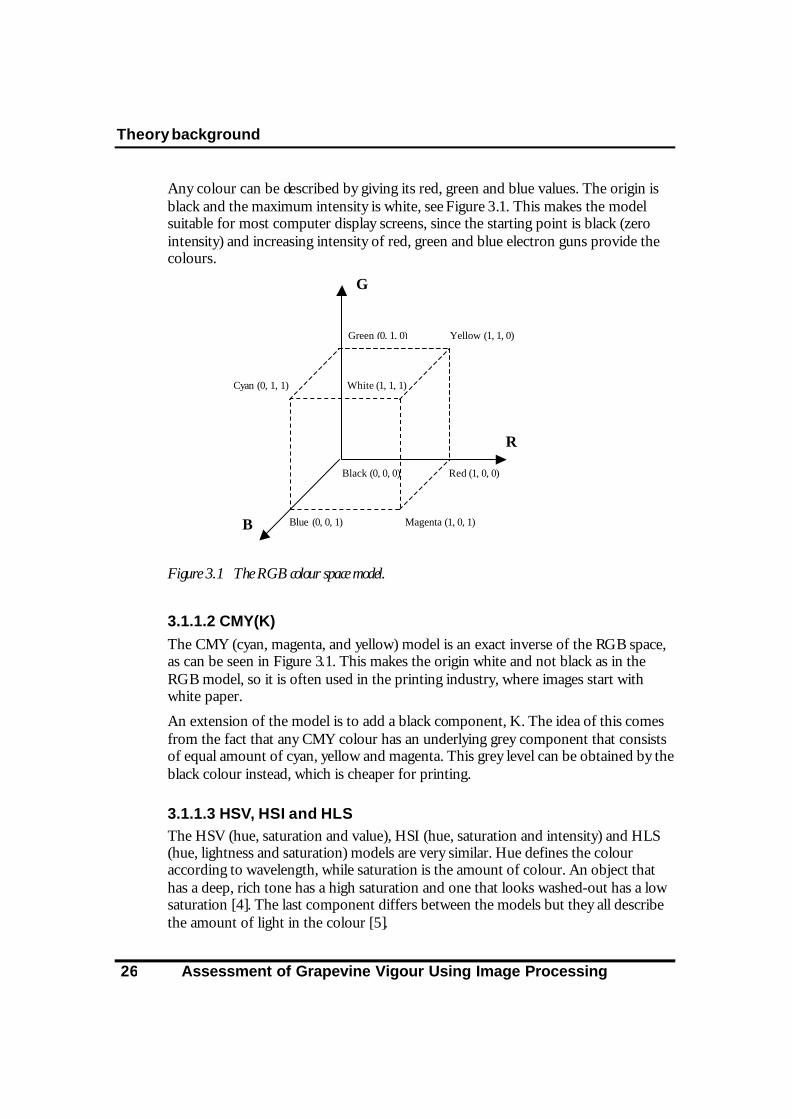
Any colour can be described by giving its red, green and blue values. The origin is black and the maximum intensity is white, see Figure 3.1. This makes the model suitable for most computer display screens, since the starting point is black (zero intensity) and increasing intensity of red, green and blue electron guns provide the colours.

Figure 3.1 The RGB colour space model.

3.1.1.2 CMY(K) The CMY (cyan, magenta, and yellow) model is an exact inverse of the RGB space, as can be seen in Figure 3.1. This makes the origin white and not black as in the RGB model, so it is often used in the printing industry, where images start with white paper.

An extension of the model is to add a black component, K. The idea of this comes from the fact that any CMY colour has an underlying grey component that consists of equal amount of cyan, yellow and magenta. This grey level can be obtained by the black colour instead, which is cheaper for printing.

3.1.1.3 HSV, HSI and HLS The HSV (hue, saturation and value), HSI (hue, saturation and intensity) and HLS (hue, lightness and saturation) models are very similar. Hue defines the colour according to wavelength, while saturation is the amount of colour. An object that has a deep, rich tone has a high saturation and one that looks washed-out has a low saturation [4]. The last component differs between the models but they all describe the amount of light in the colour [5].

R

B

G

Green (0, 1, 0) Yellow (1, 1, 0)

Red (1, 0, 0)

Cyan (0, 1, 1)

Blue (0, 0, 1) Magenta (1, 0, 1)

White (1, 1, 1)

Black (0, 0, 0)

Theory background


The HSV model will be discussed further since it is used by Matlab, the software used for this work.

The main disadvantage of the RGB model and also the CMY model, is that humans do not see colour as a mix of three primary colours. Rather, our vision differs between hues with high or low saturation and intensity, which makes the HSV colour model closer to the human colour perception than the RGB model.

Figure 3.2 The HSV colour space model.

In the HSV space (Figure 3.2) it is easy to change the colour of an object in an image and still retain variations in intensity and saturation such as shadows and highlights. It is simply achieved by changing the hue component, which would be impossible in the RGB space. This feature implies that the effects of shading and lighting can be reduced [6]. A shaded area within an object can be detected as belonging to the object, even though the shaded area is darker. The reason for this is that the hue component does not change very much with shading and lighting.

3.1.1.4 YUV and YIQ The YUV and the YIQ models are based on luminance and chrominance and are used, respectively, in the PAL and NTSC broadcasting systems and are little of interest in this project. The reason for their suitability in broadcasting systems is their compatibility with the hardware systems.

Saturation

Hue (angle)

Value

Theory background


The Y component, the luminance, corresponds to the brightness and is the only component that a black-and-white television receiver uses. The U and V (I and Q) components are used to describe the colour. The disadvantage of these models is that since only two colour components are used, not all colours that a computer screen is capable of displaying can be produced.

3.2 Matlab and colours In this project Matlab version 4.2c.1 has been used. This version of the program uses 256 colours, handled by colour maps.

When an image is loaded into the program, an RGB colour map is created (256 × 3 matrix), and all pixels in the image get an index to any of the 256 colours (i.e. rows) in the map.

The images taken with the digital camera have 24 bit colours that are approximated to 8 bits by Matlab when loaded into the program. The choice of these 256 colours is based on the statistics of the image. Since the largest areas in the images are green, the contrast in the green colour range is good, i.e. a major part of the colour map consists of green hues. Thus, the rather small number of colours, 256, is in this project enough for a sufficient resolution. Processing images with a wider range of colours would probably require the use of more than 256 colours.

Each loaded image will be assigned a colour map and it is not possible, when loading an image, to apply a certain colour map. This is inconvenient, since when working with several images it is easier if they use the same set of colours. The Matlab function imapprox approximates the images to the same colour map and provides good results, without any major distortion. The reason for this is that the images are very similar in colour. Approximating a very distinct image would result in much greater distortion.

Since the colour maps are usually much smaller than the images, any colour manipulation is a rapid process. Consider the following example:

We want to keep all green colours in an image, which is appropriate for this project. Clearing all non-green pixels in the image would force us to go through all of the image pixels, which is time-consuming when working with large images. A much faster way to do it is to simply set all non-green colours in the colour map to black, or any other appropriate colour.

3.3 Stereo A human’s two eyes perceive slightly different views of the same object, thus producing depth perception. This can be imitated by using two slightly displaced cameras capturing images of the same object. The differences in the two images are

Theory background


used and combined into a single image that explicitly represents the depths of all points in the scene.

Stereo vision can be achieved by solving two problems; the correspondence problem and the reconstruction problem [7]. What they are and how they can be solved is discussed below.

3.3.1 The correspondence problem For a point mL in one retinal plane RL, determine what point mR in retinal plane RR it corresponds to. In this context correspondence refers to the alignment of corresponding features (a physical point M) in each image. This forms the correspondence problem, which is one of the main problems in stereo vision.

The correspondence problem is solved with matching techniques, see Section 3.3.4 -3.3.6.

3.3.2 The reconstruction problem The reconstruction problem can be summarized by the following statement: Given a point mL in one retinal plane RL and its corresponding point mR in the other retinal plane RR, reconstruct the 3D co-ordinates of M in the chosen reference frame.

3.3.3 Disparity Disparity is the relative displacement between two corresponding points. The result after solving the correspondence problem is a disparity map, which is used to reconstruct the 3D co-ordinates.

To calculate the disparity of a pixel, it has to be visible and it must be identified in both images.

3.3.4 Area based matching The intensity based area-correlation technique is one of the oldest methods used in computer vision. The matching process is applied directly to the intensity of the two images.

For each pixel in one image the pixel, together with its surrounding pixels, are correlated with the other image to determine the corresponding pixel location. To a certain extent, the bigger the chosen correlation region is, the easier it is to get a correct match. Calculation time increases with region size. The disparity, see Section 3.3.3, is assumed to be constant in the region of analysis, so the result will not be accurate if too large a region is chosen.

Since all pixels are correlated, the result of the matching will be a dense disparity map.

Theory background


The drawback with area based matching is its dependency on image intensities. The images have to be captured in a way that ensures that corresponding pixels have the same intensities.

3.3.5 Feature based matching In feature based matching features, are extracted in the images prior to the matching process [8]. Features that are extracted can be edge elements, corners, line segments and curve segments that are stable under the change of viewpoint.

The drawback of this method is that a dense disparity map will not be generated since matching will only be achieved on extracted features.

3.3.6 Phase based matching In phased based matching, the fact that local phase estimates and spatial position are equivariant is used to estimate local displacement between two images. Local phase estimates are invariant to signal energy, i.e. the phase varies in the same manner regardless of the magnitude of the signal [9]. This reduces the need for camera exposure calibration and illumination control.

3.3.7 The epipolar constraint The epipolar constraint tells us that a point in image 2 of Figure 3.3, corresponding to a point in image 1, must lie on the epipolar line, which is the projection of the straight line through the physical point and the centre of projection of image 1.

Figure 3.3 The epipolar constraint.

M

m

CL CR

epipolar line for M image 1 image 2

Theory background


One way to use the epipolar constraint is to rectify the images prior to matching. With image rectification the goal is to make the epipolar lines parallel. This reduces the search for corresponding points to a one-dimensional search along the horizontal epipolar lines.

3.3.8 Other constraints To improve the matching, constraints could be used. These could either make the matching faster as with the epipolar constraint (Section 3.3.7) or provide confidence information, i.e. certainty map, which can be used to eliminate false matches. Below are some constraints given:

§ Similarity. For an intensity-based approach, the matching pixels must have similar intensity values (i.e. differ less than a specified threshold) or the matching windows must be highly correlated.

§ Uniqueness. A given pixel or feature from one image can match no more than one pixel or feature from the other image.

§ Continuity. The cohesiveness of matters suggests that the disparity of the matches should vary smoothly almost everywhere over the image. This constraint fails at discontinuities of depth, as depth discontinuities cause an abrupt change in disparity.

§ Ordering. If mL is to the left of nL then mR should also be to the left of nR and vice versa. That is, the ordering of features is preserved across images. The ordering constraint can fail at regions with no opaque surfaces.

3.3.9 Multiple view geometry A camera may be described by the pinhole model [10]. The co-ordinates of a 3D point TzyxM ),,(= in a reference co-ordinate system and its retinal image co-ordinates Tvu ),(=m are related by

=

11

zyx

vu

s P Equation 3.1

Ms ~~ Pm = Equation 3.2

where s is an arbitrary scale, and P is a 3 × 4 matrix, called the perspective projection matrix or camera matrix.

The matrix P can be decomposed as

]|[ tRAP = Equation 3.3

Theory background


where A is a 3 × 3 matrix, mapping the normalized image co-ordinates to the retinal image co-ordinates. [R|t] is the extrinsic camera parameters that define the 3D displacement (rotation and translation) from the reference co-ordinate system to the camera co-ordinate system.

The matrix A depends on the intrinsic/internal camera parameters only and has the following form

−

−

=

100sin

0

cot

0

0

vfk

ufkfkv

uu

θ

θ

A Equation 3.4

where f is the focal length of the camera, ku and kv are horizontal and vertical scale factors and are the effective number of pixels per unit length. u0 and v0 are the co-ordinates of the principa l point of the camera, i.e. the intersection between the optical axis and the image plane and θ is the angle between retinal axes. θ is introduced to account for the fact that the pixel grid may not be exactly orthogonal. In practice, however, it is very close to π/2.

The reconstruction problem in the case of two cameras is done [11] by solving

=×=×

⇒

==

0~~0~~

~~

~~

MM

MsMs

RR

LL

RRR

LLL

PmPm

PmPm

Equation 3.5

which is an over-constrained system and can be solved using a least -square technique.

3.3.10 Camera calibration Camera calibration is the procedure for determining the camera’s intrinsic and extrinsic parameters and is achieved by measuring points on a known object. The most commonly used object is a grid, where the measured points are the corners of the grid. In order to provide good 3D calibration, the grid should be positioned at several distances from the camera. The points are then used to solve an over-determined system of the projection equations for the unknown parameters.

A camera calibration toolbox is available for Matlab [12].

3.3.11 Parallel camera case In this special case, the optical axes of the cameras are parallel, i.e. the epipolar lines coincide with the horizontal scan lines, and are separated by a distance d (Figure 3.4). The cameras have the same intrinsic parameters such as focal length f. All this simplifies the description and reconstruction explained in Section 3.3.9. Triangulation will now be used to explain the reconstruction.

Theory background


Since mLcLCL, mLmM and mRcRCR, mRmM are similar triangles, the co-ordinates (x,y,z) of M are given by

)(2)(

RL

RL

xxxxd

x−+

= Equation 3.6

)(2)(

RL

RL

xxyyd

y−+

= Equation 3.7

RL xx

dfz

−= Equation 3.8

where the origin O of the system is situated mid-way between the lens’ centres (CL and CR). The pixel co-ordinates should be scaled with their metric pixel size.

Figure 3.4 The parallel camera case.

3.4 The Radon transform The Radon transform is a useful tool to find straight lines in images, so, in this project, it is useful for detection of posts, vine trunks, wires, frames etc.

The radon transform is obtained by intensity projections at different angles. Thus, the problem of detecting lines in the image turns into the problem of detecting peaks in the transform, which is much easier. The co-ordinates of these peaks

(xL,yL) (xR,yR)

(x,y,z)

f

z

x

d

M

mL mR m cL cR

CR CL O

Theory background


correspond to the parameters of the lines in the image, so the Radon domain is often referred to as the parameter domain.

The usual way of representing a line, cmxy += , is not appropriate here since m can grow infinitely large for lines that are nearly parallel to the y-axis. Instead, the line is represented in polar co-ordinates in the form

θθρ sincos yx += Equation 3.9

where ρ is the shortest distance from the line to the origin of the co-ordinate system and θ the angle of the line (Figure 3.5).

Figure 3.5 Polar representation of a line.

There are many different definitions of the Radon transform. A popular version [13] is:

∫ ∫∞

∞−

∞

∞−

−−= dxdyyxyxgg )sincos(),(),( θθρδθρ( Equation 3.10

where g(x,y) is the image and δ is the Dirac delta function. Hence, the Radon transform is the line integral, i.e. projection, over the image (Figure 3.6).

x

y

θ ρ

Theory background


Figure 3.6 The Radon transform for the angle θ, seen as a projection.

Figure 3.7 Two lines and their Radon transform. The horizontal axis of the transform corresponds to the projection angle. The vertical axis corresponds to the distance from the image centre.

The related Hough transform is used more frequently since it requires less computation. For each position in the Radon domain, a projection is performed across the image. Hence, even if the image only contains a single short line, all the projections would be performed. The Hough transform on the other hand, transforms each point in the image to a sinusoid in the transform domain.

x

y

θ ρ θ

Theory background


Therefore, an image containing only a few interesting pixels will be more rapidly transformed.

In this project, the Radon transform and not the Hough transform was used, because the Hough transform was not included in the Matlab Image Toolbox that we used. Since the approximate directions of the desired features, i.e. trunks and posts, are well known, the transform only has to be performed for a few angles, so the computational burden is considerably reduced.

Image capture


44 Image capture One objective of the project is to evaluate methods for capturing images in different lighting and background conditions.

4.1 Image background To facilitate distinguishing objects, the images need to have an easily sepa rated background. Three different background colours, magenta, white and light blue, are used, see Figure 4.1 upper row.

Magenta is complementary to green and therefore provides good colour contrast, making hue separation very successful, but the very sharp edges between magenta and green areas can cause problems for many scanners and printers.

Since white is not a hue, but comprises all hues with zero saturation and maximum intensity, an image area that appears white may have some pixels with a green hue, others with a blue hue etc. This makes hue separation inappropriate. Separation by low saturation and high value is more appropriate although the result is widely affected by bright reflections from the surface leaves.

An advantage of light blue to white is that it does not deceive the camera into overexposing as much as white does. Another advantage is the existence of a common hue, blue, making hue separation possible. However, reflections from the green canopy make the blue background appear with a green tinge surrounding the canopy. This ‘green shine’ results in noise when the canopy is separated, hence, a magenta background is the preferred option since its hue distance from green enables reflections to be ignored. However, in images captured at an early growing stage, this effect has less impact because the shoots are smaller and less green. Thus, good results are aslo achieved for white and light blue backgrounds.

Figure 4.1 Different backgrounds: White, magenta, blue, sky, cloudy and uncontrolled.

For the shoot counting, using the sky as background is an appealing alternative. Both images with a perfectly cloudy sky and a blue sky with some clouds as backgrounds were captured (Figure 4.1, bottom left and middle) by placing the camera diagonally

Image capture


below the vine and taking the photo up towards the sky. This special kind of background does not cause any problems since the sky colours are very distinct from those of the vine.

A sky background is less convenient in canopy photos. Since the rows are close together the camera has to be placed close to both the ground and the vine to have only sky as a background. Thus, not very much of the canopy will be covered in each photo. Placing the camera in front of the vine with an artificial background is more appropriate for this purpose.

Some images of the shoots were also captured from the side with an uncontrolled background, i.e. with the other vine rows behind (Figure 4.1, bottom right). To be able to distinguish the vine, the images have to be captured so that the vine with its shoots becomes much sharper than the rest of the image. That requirement is not realistic, since photographing with sufficient accuracy is not easily performed automatically. A camera mounted on a vehicle running along the row would not have the same distance to the vine all the time so that the vine will not always be in focus. It is more appropriate that the camera is directed up towards the sky so that the vine need not necessarily be in focus for successful image segmentation.

4.2 Images of shoots Light conditions and image background are not particularly important issues for shoot counting during early growth when the shoots are too small to cause major shadows or light reflections. Further, the vine is easily identified against every background that is distinct in colour, i.e. not green, yellow or brown, or much brighter than the vine. When the shoots are larger, shadows and reflections cause difficulties with analysis and are best avoided. In this case, a magenta background is most appropriate, since its distinction in hue remains even though shadows and reflections are present.

The camera is positioned at several different distances from the vine, so that the vine is covered by one to three images to provide different resolution. With a 35 mm wide-angle lens, a little more than 1 m is covered from a distance of 1 m. Since most of the vines are wider than 1 m, at least 2 images are required unless a lens with a wider angle is used. For shoot counting such a lens could be useful, since the disadvantage of wide-angle lenses - distortion in the outer parts of the image - does not seriously affect the counting. However, if accurate positioning of the shoots is required, correction for the distortion must be made. Such correction algorithms exist and are not complicated. They are not included in this work.

When an artificial background is used, the images are captured from the front. If the sky is used a s background, the images are captured diagonally from below to exclude everything but the sky as background. The angle required depends on the height of

Image capture


the vines and the distance to the vine behind. On late shoots the photos are taken diagonally from above to obtain a better view of the shoot tips (see Section 6.2).

In large-scale shoot counting, the number of shoots per vine is not required: rather, one wants the number of shoots per bay or an even coarser measure. The number of shoots per bay is appropriate since the length of a bay is fixed and can be easily expressed as an average number of shoots per metre or vine. Hence, it is not important how the vines are placed in the images, which is helpful since they are of different size.

A measure expressed in a length unit may also be obtained using projection calculations (see Equation 3.1), although the distance to the vine must be known.

4.3 Canopy images It is possible to compensate for different light sources (Chapter 8), but uneven reflections and shadows are much more awkward and should be avoided. The easiest way of reducing the impact of shadows and reflections is photographing on a cloudy day. It can also be carried out late in the day, shading the sun with the background, which then should be as non-transparent as possible. Photographing in the middle of the day when the sun is at its zenith also works well since the shadows are small and reflections are more likely to come from above rather than from the side of the canopy.

The most appropriate background colour for the canopy images is magenta. Reflections from the green canopy make white and blue backgrounds appear with a green tinge around the edges of the canopy, which results in poorer hue separation.

The side of the canopy is captured from the front. The row width (usually around 1.5 m) usually prevents the whole canopy from being included in one image, unless a wide-angle lens is used. Thus, a vine may have to be split into several images, which then are merged to obtain an image of the whole canopy. Nevertheless, the core of the canopy, i.e. excluding the protruding odd long shoots, can often be captured in one image, although this does depend on the size of the vine.

The position of the camera is not discussed further here, since it is dependent on the size of canopy, row width, mounting restraints and the focal length of the lens used. It is not very important from which position the images are captured as long as the distance to the canopy is the same in all images of a vine. They can then be merged through mosaicing (Section 4.5.2).

If the canopy cover is to be expressed in some unit of area, this can be obtained by knowing the distance from the canopy to the camera and using projection calculations (see Equation 3.1). Otherwise, canopy cover may be expressed using references in the images, for example per bay or per vine.

Image capture


4.4 Stereo Some of the stereo images were captured using two analogue cameras mounted next to each other on a bar, mounted on a tripod. This method gave poor results. Since the leaves are thin, in some cases one camera can ‘see around’ a leaf while the other cannot. The difference between the left and the right image is too large, making the correspondence search difficult (Section 7.1). Stereo imaging of such depth continuous objects as canopies requires that the lenses are closer to each other. This is not possible with normal-size cameras - smaller cameras are needed, although a stereo camera could be used. Instead, the two images are taken with the same camera at two positions on the bar, but that requires that the environment does not change from one image to the other, i.e. that wind and light do not alter the appearance of the canopy.

Stereo images were also taken as frames from a video sequence (Section 4.5.3).

4.5 Video A video camera can be mounted on any vehicle travelling along the rows of the vineyard, providing a cheap and practical way to collect large quantities of data. To achieve a sufficient distance between camera and object, the camera is most appropriately mounted on an arm protruding from the vehicle over the vine, w ith the lens directed back towards the vehicle, where the background is mounted.

4.5.1 Extracting video frames A video camera normally captures 12.5 - 60 frames per second. Analysing all frames in a long video sequence of, for example, a row of length 100 m, requires processing 625 frames, if the frame rate is 12.5 and the velocity of the vehicle is 2 m/s. The number grows with increasing frame rate and decreasing velocity. This is much more information than required and it would be a long process to analyse all frames. Instead, only enough frames to cover the entire row are required, i.e. 100 frames if each frame covers 1 m of vine. A large number of frames can therefore be cut from the sequence.

If the velocity of the carrying vehicle is constant some frames could be discarded at once, without further analysis. In the example above, using every 6.25 th frame would give exactly the information required. Using a 50 fps camera would require picking every 25th frame, but a better way is to pick some more frames, for example every sixth. The frames would then overlap, which would result in more information than needed. But on the other hand, it would allow for slight deviation from constant velocity.

Image capture


4.5.2 Mosaicing If constant velocity is not a realistic assumption, frame selection with more precision is required. A technique called mosaicing can be used. In this project, it is used to find the most appropriate next frame.

Starting with frame k, which of the consecutive frames is the one that gives us the largest amount of new information so that when the two images are merged, the size of the result will be twice that of each merged frame? Knowing the frame rate and the approximate velocity of the video camera can provide a rough estimate, such as frame k+6.25, if the velocity of the camera is 2 meters per second and the frame rate is 12.5 fps as in the example above. But, frame number k+6.25 does not exist; frame k+6 or frame k+7 must be chosen. Further, we cannot take for granted that the velocity is constant, so it is necessary to look at frame k+5 and k+8 as well, or even further, if the variation in velocity is large.

Hence, starting with frame k again, frame k+1 to k+4 are removed directly and frames k+5, k+6, k+7 and k+8 are examined further. The purpose is to find the one that best merges to frame k so that the result image covers as much vine as possible (Figure 4.2). The method is correlation. A block in the right end of frame k is correlated horizontally in each of the three frames. The frame that has a hit further to the left is chosen. Ideally, the next frame should not have any common information with the first frame, but the correlation requires that some part of the vine is in both frames, even though the common part should be as small as possible to avoid redundant information.

A slightly different method would be to pick frames a little more frequently than required and find where they align. In the example, every fourth or fifth frame could be chosen. The maximum correlation (performed in the same manner as above) would occur where every new frame fits to the previous. The total amount of image data would be larger compared to the other method, since some image information would be redundant, but it would run faster.

Image capture


Figure 4.2 Mosaicing. Two frames from a video sequence are merged into one image. The frame that together with the first frame covers most of the vine is chosen.

When a row ends a problem occurs since he frames from outside the row are not required. How can this automatically be detected? One way would be to mark the beginning and end of each row and implement an image analysis algorithm that detects these marks. They could even contain some detectable index to keep track of the rows in the video sequences.

4.5.3 Video sequences for stereo images The stereo image method of estimating the canopy cover of a vine requires two frames per vine or per section of vine. If stereo imaging with more than two images is used for improved accuracy, it is easy to extract more frames.

Selecting frames can provide control of the distance between the left and right images, thus avoiding the problem of a too large distance between two mounted still cameras. The distance can be approximated by knowing the velocity of the camera. If the velocity is constant, the result is good, but if it deviates too much the result gets worse. In the latter case, the velocity can either be calculated by detecting references in the images or by using a high precision speedometer.

Picking frames from a video sequence adds more insecurity to the depth calculations but it is a practical and realistic capturing technique. The major difficulty, besides knowing the distance between the frames, is to align the images since the movement of the video camera is not perfectly even. Some frames may be skewed, although

Image capture


skewing is unlikely if the camera is mounted on a vehicle. There will also be differences in height of the frames but they should be small and easily rectified. It is not absolutely necessary that the frames are at the same height for the stereo algorithms. However, if the left and right images only differ horizontally, the algorithms will run faster since vertical correspondence searches need not be done. This could be achieved by using two parallel video cameras.

4.6 Image resolution The video sequences captured in this project have a resolution of 320 × 240 pixels. That is sufficient for the most resolution demanding process, stereo imaging. It is also an appropriate resolution for other processes, su ch as the canopy density algorithms and the shoot counting algorithms. However, less than half the resolution, 150 × 100, is sufficient shoot detection by colour separation, but it does require that images are captured from a maximum distance of approximately 0.5 m.

In a practical system, the images could be captured in 320 × 240 and decreased for processes that achieve a sufficiently good result with lower resolution, thereby providing increased processing speed.

Image segmentation


Image segmentation


55 Image segmentation

5.1 Colour separation techniques When separating colours, one usually looks at the histogram of the image, to study the distribution of pixels over the colour spectra. The histogram may have clearly separated parts, making it easy to find threshold values that achieve the separation, but in most cases when dealing with natural images, there are no obvious separation thresholds since the pixels are spread all over the colour spectra. However, there are a number of methods to find threshold levels that minimise incorrect classification. These include:

§ Local thresholding [14]

§ Iterative thresholding [15]

§ Optimal thresholding [14], [15]

In many cases though, the image can be coarsely separated into groups of colours. For example, in our case, a typical image of a vine may be separated into the green canopy, the brown trunk and the background. This is considered sufficient for the purposes of this project. Three methods have been tried for this coarse separation: separation in the RGB space, separation in the HSV space and intensity separation. In each case, the classification is performed on the colour map rather than on the indexed image, since the colour map is much smaller.

5.1.1 Separation in the RGB space By setting up requirements on the proportions of the pixels’ three colour components (r,g,b) and their magnitude, each pixel can be classified as either belonging to an object or not. A typical set of requirements for green colour separa tion is:

ui

btgrsg

>>

>

**

Equation 5.1

where r, g and b are the RGB components of a pixel, s and t the proportion of green colour to red and blue colour, i the intensity of the pixel and u the required intensity level. An example of this is presented in Section 5.3.

5.1.2 Separation in the HSV space Separation in the HSV space is most relevant to this work. Particularly important is the hue, since it is not affected by shadows and reflections. It also reflects very well

Image segmentation


the coarse perception of colours that is very useful in this work. For example, the canopy can be classified as just a hue range, not as a large range with three components as would be the case in RGB separation. Separation along the hue vector is just a matter of finding the range in the hue spectra (Figure 5.1) that represents each colour group, e.g. green in the approximate range 0.2 to 0.45.

Figure 5.1 The hue spectra.

5.1.3 Separation by intensity Separation by intensity has also been useful in this project. It has been used mainly to remove a background that is much brighter than the rest of the image (Section 5.2.1), but has also been used to differentiate between objects, such as trunks and posts (Section 5.5).

5.2 Background removal Removal of the background is a straightforward procedure. The background can be characterized either by its intensity or by its colour.

5.2.1 Separation by intensity One way to detect the background is by user interaction. The user marks the background, either by clicking the background in a number of places in the image or by dragging a square of the background. The mean and standard deviation of the grey-scale image are then calculated for the pixels collected and every pixel with intensity within a number of standard deviations from the mean intensity of the background are set to black.

A second method uses the fact that the majority of the pixels belongs to the background and can therefore only be used when that is the case. Thus, this approach is appropriate for shoot counting but not for canopy description where the canopies cover most of the image. Pixels whose intensity is within a certain distance from the intensity histogram peak are removed.

The major disadvantage of these methods, besides the need for user interaction is the fact that many pixels belonging to the canopy or shoots have an intensity close to that of the background. The result is removal of some relevant pixels. Further, these methods require that the background is evenly lightened, which due to shadows, is not always the case.

Image segmentation


If a sequence of images is captured under identical conditions, the procedure only has to be performed on one image, since the background will have the same appearance in all images.

A requirement for achieving a good result is that the intensity of the background is as distinct as possible from that of the vine. This applies to both methods, usually requiring a bright background, even though, as mentioned above, this may not ensure perfect separation.

5.2.2 Separation by hue The third method is the most convenient and also one that gives the best result, provided the images have been colour corrected. It separates the background from the rest of the image in the HSV colour space and is therefore less susceptible to shadows and other noise in the image background. It requires though that the background has a hue that is distinct from that of the vine.

The hue component histogram has two distinct peaks (Figure 5.4) that represent the canopy and the background. The background removal is simply achieved by removing all colours from the colour map that have hues in a specific range, representing for example light blue or magenta, or whatever colour the background might be.

In images with no more than a background and a vine, background removal will be the same as segmentation of the canopy (see Figure 5.5).

5.2.3 Results None of the single coloured white, light blue, magenta or evenly cloudy sky backgrounds are difficult to remove using any of the three methods. The hue separation method also successfully removes any background that is not evenly coloured, e.g. a blue sky with clouds, as long as the background hues are separated from the vine hues. The blue/cloudy sky can also be removed with an ad hoc method that finds the clear sky pixels by their dominating blue component and the cloud pixels by their high intensity.

All methods remove colours, i.e. set them to black, from the colour map and do not change the indexes in the image. This makes them execute rapidly since the size of a colour map is only 256 × 3 compared to at least 100 × 150 for the indexed images. As a result, several of the colour map indexes in the image will point to black.

The result is worse for uncontrolled backgrounds. Images w ith no controlled background, i.e. with the vine rows behind as background, do not provide satisfactory results since processing time is excessive and produces mediocre results. The background can be removed, or rather the vine extracted, but under the requirement that the images are captured so that the vine is sharp and the rest of the

Image segmentation


image blurred. Edge detection algorithms can then extract the vine. However, the resolution and the image capturing accuracy have to be high, which probably makes this option impractical.

Separation by hue is the most successful of the methods, because it usually provides the most satisfactory result. It allows the background to have some colour variation, caused by shadows, reflections and uneven lighting. If the background is magenta-coloured the result is almost perfect.

5.3 Extraction of shoot and canopy The fact that the leaves, as well as the shoots, are green and the rest of the pixels in the image tend to have other colours makes it appropriate to use colour separation to distinguish leaf pixels from other pixels. In the RGB colour space it is not only leaf pixels that have a green component. In fact most pixels have a non-zero green component even though they do not appear green. Thus, a colour range has to be defined so that pixels that lie within the range are classified as leaf pixels.

A simple way [16] to separate the green objects (shoots or canopy) from the rest of the image is to classify all pixels with green as the dominant component as leaf pixels, i.e. any pixels with g > r and g > b. This works surprisingly well for many of the canopies. It is often desirable though to also require that the g component have a certain level of dominance. This is achieved by extending the classification set to let pixels with g > s*r and g > t*b, where s,t > 1, represent the shoot colours (Section 5.1.1).

However, a more appropriate method is to separate the shoots or the canopy by hue. The histograms in Figure 5.3 and Figure 5.4 show that conversion of typical canopy images ( Figure 5.2) to the HSV space facilitates finding thresholds. There is an obvious separation of the different hues in the image.

The result from hue separation of some images is shown Figure 5.5. Green colours are approximately in the range 0.2 to 0.45 (Figure 5.5, upper middle and upper right). At early stages of growth, the shoots have more yellow and brownish hues in the range 0.1 to 0.2 (Figure 5.5, upper left).

Depending on factors such as light conditions and camera equipment, the hues may change slightly from image to image. If the variation is too large, i.e. if it is difficult to define a hue range, a colour correction (Chapter 8) can be performed a priori to reduce the noise.

Image segmentation


Figure 5.2 Two canopy images with different backgrounds, light blue and magenta. Their histograms are shown in Figure 5.3 and Figure 5.4.

Figure 5.3 RGB histograms of the images in Figure 5.2.

In later growing stages, shoot detection may be difficult using only colour separation (see Section 6.2).

Image segmentation


Figure 5.4 HSV histograms of the images in Figure 5.2. Appropriate threshold levels are much easier to find here than in the RGB histogram. The canopy hues are found around 0.2 and the light blue background hues (left) around 0.5. The magenta hues (right) at around 0.95 are very distinct from the vine hues.

Figure 5.5 Shoot and canopy segmentation by hue separation.

5.4 Extraction of fruit clusters Grape varieties that are used to produce red wine have a dark blue fruit that is easily separated from the rest of the image, since no other blue colour appears on the vine.

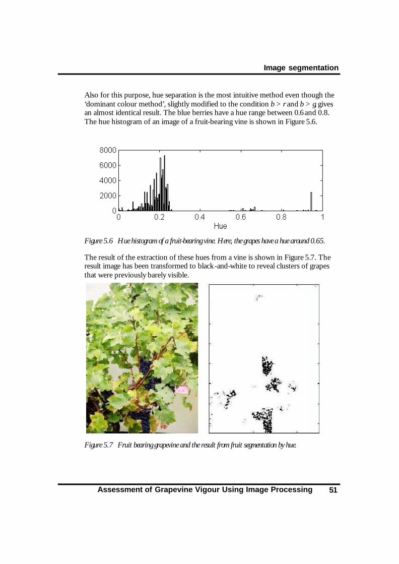
Image segmentation


Also for this purpose, hue separation is the most intuitive method even though the ‘dominant colour method’, slightly modified to the condition b > r and b > g, gives an almost identical result. The blue berries have a hue range between 0.6 and 0.8. The hue histogram of an image of a fruit-bearing vine is shown in Figure 5.6.

Figure 5.6 Hue histogram of a fruit-bearing vine. Here, the grapes have a hue around 0.65.

The result of the extraction of these hues from a vine is shown in Figure 5.7. The result image has been transformed to black -and-white to reveal clusters of grapes that were previously barely visible.

Figure 5.7 Fruit bearing grapevine and the result from fruit segmentation by hue.

Image segmentation


5.5 Post and trunk detection Posts separate the bays of a row and hold the trellis wires that support the vines. It is useful to detect them, since the measurements often are expressed per bay. For example, in a video sequence of a row, the beginning and end of a bay can be detected and the number of shoots or a measure of the canopy cover can be calculated for that bay.

The posts are made from metal or wood, but detection using colour characterization is not easy. Grey is an equal blend of the RGB components, but, looking at separate pixels, one may have a red tinge and another may have a green tinge etc. due to the camera and the resolution that has been used. Together they make up grey so it is difficult to find a specific range of RGB combinations that represent grey. A conversion to the HSV space does not improve the situation. Grey is not a hue; it is any hue with little saturation. The near zero saturation could be used to characterize a post, but there might be other pixels in the image that have a very low saturation, for example bright leaves.

A wooden post cannot easily be detected by this method either, in this case due to the wide variation in colour. Both the wooden and the metal colours have vague hues that do not allow a good hue sepa ration result.

A more appropriate solution is detection by shape. Posts and trunks have unique shapes that separate them from other objects in the image. They are both straight and long with sharp edges. Further, posts are vertical although trunks are usually non-vertical.

Many methods exist for detecting long, thin objects in an image, but any evaluation of these methods is not within the scope of this project. Thus, only one method has been used. It includes the following steps:

1. Vertical edge detection in the grey-scale image.

2. Removal of the leaf edges.

3. Radon transformation of the edges.

4. Finding the maximum points of the radon transform.

The vertical edge detection is achieved by the Sobel method on the grey-scale image. Many of the detected edges are located in the canopy (Figure 5., left). Since many shoots are long and thin they might be mistaken for posts, so the leaf edges are removed by multiplying the binary edge detection image with a mask (Figure 5., middle), which is produced by separating the canopy from the original image and transforming it to a binary image. Figure 5. (right) shows the result of the removal of the canopy edges.

Image segmentation


Figure 5.8 Left: Result from edge detection. Middle: Mask used to remove the leaf edges. Right: Result from masking of the left image.

Figure 5.9 shows the Radon transform of the right image in Figure 5.. The horizontal axis shows the angles for which the intensity projections have been performed (Section 3.4) and the vertical axis shows the horizontal position in the original image, where the projection has been made.

Figure 5.9 Radon transform of Figure 5. right.

The dark spots indicate a high projection sum. The right-hand image in Figure 5.9 shows the Radon transform for angle 90° only. The highest peaks correspond to the edges of the post and its horizontal position can be established.

Only methods for finding the post in an image that knowingly contains a post are developed. For automatic detection of posts and trunks in a sequence of images a decision rule has to be set up, but we confine ourselves to a brief discussion on how this could be achieved.

Since the visible part of posts and trunks may differ in size between images, it is not efficient to require that the Radon projection sum must be of a certain size to be classified as a post or trunk. Occasionally a post can be almost fully hidden in the canopy and sometimes the entire post is visible. The decision rule must be relative to some characteristic of the image. The only objects in the image that have relatively long edges after removal of the canopy are the posts and the vine trunks. Hence, the Radon projection sum will be much larger along them than for the rest

Image segmentation


of the image, even though only small sections are visible. Thus, if any projection sum is much greater than other projection sums, it most likely represents a post or a trunk at that position.

In an application that processes a large amount of data, finding the posts and trunks by using the Radon transform of the entire image is inefficient and unnecessary. Given that they are visible in the bottom of the image, it suffices to look at a horizontal strip at the bottom of each image to make the algorithms run faster.

If there are two dominant peak areas in the Radon transform, taking in account that both a post and a trunk cause two peaks each, there is most likely one post and one vine trunk in the image. They can then be separated by their colour or intensity difference. The trunk is usually darker.

If it is only required to identify the trunk, colour detection in the lower strip of the image is worth considering, since it is requires less computation.

Shoot counting


66 Shoot counting The objective is to find image processing techniques that can replace the tedious work of manual shoot counting and maintain a reasonable accuracy. Detection methods have been tried on different stages of the growth cycle. The shoots change very rapidly and one vine may have shoots with totally different appearance, which resulted in an ad hoc development process for the algorithms.

6.1 Shoot detection during early growth Shoot counting during early growth, need contend with few obstructing leaves, making manual counting possible using just one viewpoint. It is therefore a reasonable assumption that image processing using a single image of the vine should provide satisfactory results.

6.1.1 Shoot colour separation When buds have just burst they are easy to count by recognizing each leaf-coloured area as a shoot. The parameters for the colour separation will have to be changed according to the colour of the shoots, which depends on the variety and other factors. They often have a yellow -brown tinge when very young and become greener during growth. Therefore a certain degree of red and green dominance over blue is a good criteria for separation. Hue separation also works well. Young shoots in the test images of this project have a hue between 0.1 and 0.2, i.e. yellow.

Since the trellis wires or cane usually cover some of the shoots, they will be split in the colour separation. After a transformation of the leaf separation result to black and white, dilation is performed to join the split sections so that one shoot is not mistaken for two. The results are shown in Figure 6.1. However, two shoots growing very close to each other may be counted as one since they are merged by the dilation. Since perfect accuracy is not important, that problem is not an issue.

The procedure works well with a resolution as low as 150 × 100 pixels. A lower resolution results in the risk that small shoots are not counted, as they may be made up of only one or a few pixels and regarded as noise.

Shoot counting


Figure 6.1 Result from shoot detection by leaf colour separation. A vine (upper) is leaf colour separated (middle) and dilation is applied (lower).

6.1.2 Extracting the cane A little later in the growing phase, when the shoots are a few centimeters long, some shoots that grow together appear as only one in the colour separation process. Hence an alternative algorithm has been developed that extracts the cane by its dark colour and detects the spurs. The following steps define it:

1. Extraction of the cane by colour or intensity separation.

2. Transformation to binary image.

3. Morphological operations: dilation, erosion and thinning to produce the skeleton of the cane.

4. Detection of spurs (line ends).

5. Validity control.

Unfortunately, difficulties with stages 3 and 4 prevented consistently good results from being obtained. The outcome of the skeletonization (see Figure 6.4) markedly affects spur detection. The Matlab Image Toolbox skeletonizing function is not used, since it produces a skeleton that is too fine, while only a rough skeleton is required.

Shoot counting


Figure 6.2 shows the 3 × 3 pixel patterns that have been recognized as spurs. The algorithm uses a look-up table (LUT) for the detection and the result for the vine in Figure 6.3 is seen in Figure 6.4.

Figure 6.2 Pixel formations for spur detection.

Figure 6.3 Low-resolution image of a vine in early shooting stage.

Figure 6.4 Upper left: The cane has been extracted by intensity separation. Upper right: The vine skeleton is obtained after dilation, erosion and thinning operations. Lower left: The line ends are detected by pixel pattern matching. Lower right: A validity check.

0 0 0 0 1 0 0 0 0 0 0 01 1 0 0 1 0 0 1 1 0 1 00 0 0 0 0 0 0 0 0 0 1 0

1 0 0 0 0 1 0 0 0 0 0 00 1 0 0 1 0 0 1 0 0 1 00 0 0 0 0 0 0 0 1 1 0 0

Shoot counting


The procedure works well as long as the skeletonization succeeds in thinning all spurs protruding from the cane into single-pixel lines, without any ‘spurs on spurs’. That is a stringent requirement for the skeletonization process. Instead, it is better to use more advanced pixel patterns of larger size such as to detect the line crossings instead of the ends, i.e. detect the nodes where the shoots grow from the cane. This would require larger pixel patterns since the crossings can have many different shapes that a 3 × 3 pixel pattern cannot represent.

Further aspects are that a line end does not necessarily represent a shoot, and the ends of the cane or other protruding objects are detected. Hence, there is a need for a validity check after detection. One solution is, for example, to require that the detected pixels have an environment that is leaf-coloured. This is applied as the ‘validity check’ on the lower right image in Figure 6.4.

6.2 Shoot detection during lather growth Manual shoot counting at a late stage involves viewing shoots from different angles and distances and even moving some shoots aside to obtain a clearer view. The most appropriate characteristic to look for during manual inspection is the stem. However, this procedure is impractical for an automated method using image processing and another approach is required.

The feasibility of using the shoot tip as a characteristic feature is investigated here. A shoot tip has a red tinge and is brighter than the rest of the shoot. Two different approaches are investigated, that utilize each of these two characteristics to extract the shoot tips by colour separation. To facilitate this, images are captured diagonally from above for at better view of the shoot tips. The four images in Figure 6.5 are used to show the procedures and results.

The major difficulty is that the appearance of shoots is quite variable, whether on the same or different vines, making it difficult to find robust separation conditions.

Shoot counting


Figure 6.5 Test images for shoot detection in later growing stages.

6.2.1 Red tip detection A shoot tip has a red tinge and this characteristic is used here for detection. Other areas in the image also have slightly red tinge, but not with as high a pixel concentration as the tips. The detection procedure is:

1. Separate red pixels by hue.

2. Use median filtering to keep only high concentrations of red pixels (Figure 6.6).

3. Dilate to merge divided tips (Figure 6.7).

The method works well for some images (compare Figure 6.5 and Figure 6.7) where the shoots are clearly reddish and easy to see, in which case the parameters are easily adjusted to obtain a generally robust solution. However, it fails in images where some shoots are obscured.

Shoot counting


Figure 6.6 Median filtering. The result is obtained by median filtering the red separation result using a 3 × 3 kernel. The median filter keeps high concentrations of pixels and removes noise.

Shoot counting


Figure 6.7 Dilation. After median filtering, a dilation function is applied to the binary image to merge the split red areas.

6.2.2 Bright leaf detection Apart from the tips having a red tinge, leaves near the shoot tip are also brighter green than the rest of the canopy. This provides the possibility of detecting a shoot, but unfortunately some shoots also have bright green leaves growing beneath the tip. Therefore conditions have to be added to prevent a shoot from being detected more than once due to several light green areas. One way would be to only recognize one shoot per vertical section of the image.

The procedure for bright leaf detection is:

1. Separate bright green pixels by hue and value (Figure 6.8).

2. Use median filtering to keep only high concentrations of bright green pixels.

3. Dilate to merge split parts (Figure 6.9).

The colour of the shoot tip leaves is, in the RGB space, predominantly green with a relatively high intensity. A colour separation method that filters colours with these two characteristics provides a reasonable result, but the colour range is easier to

Shoot counting


describe in the HSV space. Here, all of the canopy will have approximately the same hue and parts of the image with other hues can be removed using hue separation (Section 5.1.2). A further separation of the canopy is achieved by either saturation or value. Bright leaves have lower saturation and higher value than the rest of the canopy. Figure 6.8 shows the result from separation by hue and value of the four test images in Figure 6.5.

Figure 6.8 Bright leaf colour separation. The four test images have first been hue separated, then value separated.

Shoot counting


Figure 6.9 Dilation. The median filtered result images from the hue and value separation are dilated to merge split parts.

As seen in Figure 6.9, the result after dilation, this method does not find all the shoots and, as expected, some shoots are detected twice.

6.2.3 Correlation with internode Detection of the shoot stems through correlation with part of a stem, e.g. an internode, gives a result that depends on the visibility of the shoot stems. The problem is that the shoot stems are split into fragments due to leaf covering. Further, since the shoots are orientated at different angles, the correlation has to be performed several times with a rotated piece of stem. The method does not give particularly satisfactory results and is computation is slow. Therefore, further development and discussion of the method is not made.

6.3 Conclusion The main difficulty with developing rugged shoot counting techniques is the great variance in the appearance of a shoot. Algorithm A may find the majority of the shoots but miss a few and detect a few extras that are not shoots but other objects.

Shoot counting


Algorithm B or algorithm A with different parameters may find those shoots that were missed but miss others. Hence, it is difficult to develop algorithms that find all shoots, in all circumstances. Image processing algorithms cannot perform actions used in manual counting, such as taking a step closer, moving some shoots aside or looking from another angle.

However, combining different techniques and calibrating the parameters for each set of images that are to be analysed can achieve a reasonable result. For example, the ‘red tip’ and ‘bright leaf’ algorithms may be combined and provide good results (better than ± 20 % accuracy) with some calibration.

Nevertheless, the best solution is the simplest. Shoot colour separation is by far the easiest and quickest method and also gives the best results, but requires that shoot counting is performed at an early stage, when the shoots are still clearly separated.

Cane extraction is a demanding and overly complicated process, at least for the images used in this project. However the technique could be useful for other purposes, such as vine shape assessment.

Canopy density


77 Canopy density The density of a canopy can be interpreted in several ways. Within vine management, it is mostly estimated using a visual assessment, the PQ (Section 2.4.1) or the LIDAR method (Section 2.4.2). PQ and visual inspection estimate the number of leaf layers as a measure of canopy density, while LIDAR uses the physical depth (i.e. the surface profile) of the canopy. The assessment methods developed in this project have slightly different approaches, according to what is possible with image processing.

Recall that the camera takes images of the side of the canopy, from between the rows. Then, estimating the percentage area of leaves in the 2 -D image plane is straightforward, but obtaining a consistent measure of canopy depth (from the camera viewpoint) is more difficult. By looking at the image, the human eye can assess the canopy’s depth. What details in the image make that possible? One is that we tend to regard dark leaves as being further into the canopy than bright leaves. This can in many cases be regarded as true due to two facts: less light reaches the inner parts of the vine and new leaves are brighter and are situated at the surface of the canopy. During the growing season, the vine produces new bright leaves continuously at the surface while the old ones darken and finally wither. The fact that leaves are shading and covering each other reduces accuracy of a method using this principle since it is difficult to know if a dark leaf is deep into the canopy, shaded by another leaf or perhaps withered. Despite these drawbacks, a coarse estimation should be possible.

In this chapter, several different methods to estimate the canopy density have been devised and evaluated.

7.1 Depth estimation using stereo This method estimates the depth of the canopy through a stereo image pair, and should provide the same result as LIDAR. The emphasis is to investigate the possibility of using stereo. There are several possible techniques to choose from when working with stereo, but in this study the algorithm is kept as simple as possible.

7.1.1 Procedure The cameras are assumed to be parallel, which makes rectification (Section 3.3.7) straightforward since only vertical alignment is necessary. When using monocular stereo images from a video camera this is not strictly true but the results are adequate. Rectification uses a correlation-based method to find corresponding points in the image.

Canopy density


Matching fails on areas with poor texture, so the background in the disparity image will have incorrect values. To avoid this, the background can either be removed prior to or after the disparity calculation. The background is removed after the disparity calculation by multiplying the disparity image with a binary mask of the canopy.

To find matching points in the images, different correlation methods are tested. However, the fact that the thin leaves may appear as having different shapes between images, due to the discontinuities in depth, makes matching difficult. The technique that gives the best result is an area based correlation technique, however with a more sophisticated algorithm it should be possible to get more accurate results.

Since the images are aligned, only a one-dimensional correlation is needed, but to improve matching, a two-dimensional correlation window is used. Only a rough disparity map is needed so disparity is not calculated for every pixel in the images but is instead calculated for whole regions, which speeds up the algorithm significantly. A restriction associated with this window-based approach is that the size of the correlation windows must be carefully chosen. If the correlation windows are too small, the intensity variation in the windows will be indistinct and false matches may result. If the windows are too large, resolution is lost since neighbouring image regions with different disparities will be combined in the measurement. When working with images of resolution 240 × 320 pixels that cover one vine canopy, the region that is used is 10 × 10 pixels and the best result is obtained with a matching kernel of 20 × 20 pixels.

An improvement would be to only match those regions in the images that are ‘interesting’, for instance, regions that contain a large variation of intensity values in the horizontal, vertical, and diagonal directions. The simple Moravec’s interest operator [17] detects such regions from the image pair.

To further improve and speed up the algorithm a hierarchical coarse-to-fine approach [18] is used. This is based on an image pyramid of the stereo pair. The correlation starts at the top of the image pyramid by selecting a window in the right image and then searching for that window in the left image. The estimated positions are then transferred to the next lower level. At this level the transferred position is used to limit the search space.

The images in Figure 7.1 are captured at a distance of 165 cm from the centre of the vine, i.e. the wires, and the canopies are approximately 20 cm closer to the camera than the wires. In all images, except one, there are shoots that are much closer to the camera, marked by red circles. Those shoots are approximately 90 - 100 cm from the camera.

Canopy density


Figure 7.1 Canopy images. Red circles point out areas that are more than 30 cm closer to the camera than other regions.

Figure 7.2 shows the depth images of the canopies, where the stereo images have a separation of 8 cm. The shoots that are closer to the camera are easily distinguished.

Canopy density


Figure 7.2 Depth images of images in Figure 7.1 with distances in cm from cameras.

A median filter on the disparity image can be used to eliminate possible mismatches, see Figure 7.3.

Canopy density


Figure 7.3 Median filtered depth images of images in Figure 7.1 with distances in cm from cameras.

7.1.2 Accuracy To investigate the accuracy of stereo, the image in Figure 7.4 is used. There are four different objects at different distances to the camera.

Canopy density


Figure 7.4 Test image, sunglasses 50 cm, mobile 70 cm, clip 90 cm and mug 110 cm, from the camera.

Images are captured at four different horizontal positions to form three stereo pairs with camera separation distances of 6 cm, 8 cm and 10 cm.

Area based correlation is performed on edge-extracted images, using Sobel kernels. The resolution of the images is 240 × 320 pixels, the matching kernel is 20 × 20 pixels and the depth images are median filtered with a 3 × 3 kernel.

Figure 7.5 Depth maps with different camera separations, left 6 cm, middle 8 cm and right 10 cm.

As can be seen in Figure 7.6 the result for 6 cm camera separation differs from the expected result. One possible reason is that the actual separation is less than 6 cm. The median filtering also affects the result, but the main reason is that with small camera separations, in the case of the mug, a difference in disparity of one pixel causes a difference in depth of 20 cm.

Canopy density


0

50

100

150

200

Sunglasses Mobile Clip Mug

6 cm8 cm10 cm

Figure 7.6 Depth with different camera separations.

7.1.3 Video With a digital video camera, a sequence of images can be captured by moving the camera horizontally. From this sequence two frames are chosen to calculate the disparity.

Figure 7.7 Image sequence where two frames are extracted.

This gives a result that is better than expected. However, since the camera’s horizontal velocity can be difficult to measure, the exact depth cannot be calculated correctly. This will not be a problem if the camera is always moving with the same velocity, since the useful information is the depth relative to other canopies.

7.1.4 More images When using a video camera for image capture, it is easy to extract more images than strictly required and to use these to increase accuracy.

Canopy density


In most trinocular stereo algorithms, potential correspondences are hypothesized using two of the images, then confirmed or rejected using the third. Okutami and Kanade have proposed another method [19], which finds matches by using all images at the same time.

7.2 Total leaf cover The easiest way to get a measure of the mean canopy density is by calculating its cover. The main assumption in this method is that there is a direct relationship between leaf area in the image plane, and the canopy density. If there are few and small gaps, the canopy is likely to be dense and have appreciable depth. If there are many and large gaps the canopy is likely to be thin. This implies that this method of measuring canopy density is closely related to the measurement of gap percentage (Section 9.1).

The assumption holds until there are no gaps at all in the canopy and leaves fill the entire image or region of interest. Then, there can still be a variation in number of leaf layers or thickness that will not be seen using this method. Further, large leaves at the front of the canopy may cover the entire region and obscure the number of leaves.

Figure 7.8 Total leaf area extracted. Top: Thick canopy. Bottom: Thin canopy.

Canopy density


It needs to be mentioned that this method does not give as accurate results on number of leaf layers as does a PQ measure, since it cannot determine the actual number of leaf layers but assumes a close relationship between the number of leaf layers and the area of cover.

The idea of the method is to calculate how much of the image is comprised of the canopy. First the canopy is segmented and then an area calculating function is applied. Either the bwarea function included in Matlab Image Toolbox or simply a count of pixels can be used. The bwarea function does not calculate two diagonally adjacent pixels as an area of 2, but estimates the area by applying a filter. The images are large, so counting pixels does not significantly reduce the accuracy, but for convenience the toolbox function is used here. The result is that the canopy area for the thick canopy of Figure 7.8 is 78 % and for the thin canopy 51 %

With a calibrated camera (Section 3.3.10) positioned at a known distance to the canopy the leaf area can be expressed in m² or any other area unit using projection calculations (Equation 3.1).

7.3 Local leaf cover Local leaf cover is no more than the ‘leaf area’ method discussed before, with the image divided into smaller blocks or regions. The local green area is calculated which provides us with information on the density of leaves in different parts of the canopy. Where the canopy has gaps the local area will be small, whereas in dense areas, the local area will be large.

Canopy density


Figure 7.9 Local leaf cover for different region sizes.

Figure 7.10 Local leaf cover for different region sizes.

100%

0%

100%

0%

Canopy density


If the regions are small, the correspondence with the PQ measures will be significant. The PQ records the number of leaves that touch a rod at a number of positions over the canopy. Imagine a small region around each of these positions. The larger the leaf area of that region, the greater the likely number of touching leaves. The major source of error is the fact that the rod is pushed through any leaf that comes in its way and in that way actually ‘sees behind’ the leaves. That is not possible with image analysis. On the other hand, the PQ method measures the number of leaves at only a limited number of positions while image analysis utilizes the information stored in the surrounding pixels as well.

7.4 Intensity changes An algorithm has been developed that utilizes the changes of intensity in the canopy. Where the canopy is dense, there are usually more colour changes through the canopy since the layers tend to have different intensities, with the inner layers having the darkest colours.

This algorithm counts the number of colours in smaller regions of the image and is used as an estimate of the number of leaf layers. But 256 colours inappropriately allows small colour changes within areas that seem to have the same colours. A reduction to only 5 colours is therefore done first.

The approximation to 5 colours uses the Image Toolbox function imapprox, which uses an image histogram to best approximate the 5 colours. In that way, the chosen colours are close to those most represented in the original image, which should make a certain layer appear in less, ideally only one, colour. Imapprox imitates colours that are not in the colour map by combining two other colours. This will fool the algorithm, so the image is first converted to greyscale and is median filtered. A threshold level is set, to further avoid counting colours other than the main colours. For a colour to be counted in a region, it must make up a certain pixel percentage of that region.

The results of this method on small leaf areas are shown in Figure 7.11.

Canopy density


Figure 7.11 Result of the ‘intensity changes’ method on small areas. Left image is counted as one leaf, middle image as two leaves and right image as three leaves.

Dividing the image into very small regions is likely to produce a less accurate result. The idea of the method is to cover le aves at different depths in one region and that will not be the case if the regions are too small. The results for some resolutions are shown in Figure 7.12 and in Figure 7.13, where the canopies used are the same as in Section 7.2. The image of the thin canopy was taken in sunshine, which causes reflections in outer leaf layer, but it is preferable that this should be avoided.

Canopy density


Figure 7.12 Thick canopy. Upper left: The image is approximated to five colours and converted to grey-scale and median filtered before counting of colours. Upper right: Result for 40 × 40 region size. Lower left: Result for 20 × 20 region size. Lower right: Result for 10 × 10 region size. The brighter the pixel, the thicker the canopy.

4

3

2

1

0

Canopy density


Figure 7.13 Thin canopy. Upper left: The image is approximated to five colours and converted to grey-scale and median filtered before counting of colours. Upper right: Result for 40 × 40 region size. Lower left: Result for 20 × 20 region size. Lower right: Result for 10 × 10 region size. The brighter the pixel, the thicker the canopy.

As can be seen in Table 7.1 the leaf layer number decreases with region size.

Region size

Mean layers thick canopy

Mean layers thin canopy

40 × 40 1.71 1.10

20 × 20 1.57 0.94

10 × 10 1.30 0.81

Table 7.1 Mean of number of leaf layers for different canopies and region sizes.

The implementation of this method has been simple and although it works well, there are many ways in which it could be improved. Some calibration is required to obtain a result comparable to the PQ measures. An improvement would be to only allow colours that differ by a certain amount, i.e. when the colour reduction is done colours are picked so that the colours are not too similar. Another improvement would be to look at local maximums in the histogram when selecting colours.

4

3

2

1

0

Canopy density


A reasonable assumption is that this method will not work well on canopies that have reached a certain thickness. It will not be possible to see all leaf layers, since some will be totally hidden behind the outer ones.

7.5 Comparison with Point Quadrate Figure 7.14 shows the PQ results on the canopies used in Sections 7.2, 7.3 and 7.4. The PQ was performed according to [2] and the measurement used 48 insertions.

The mean number of leaf layers is calculated by dividing the total number of leaf contacts by number of insertions. For the thick canopy (Figure 7.12) this is 84/48 = 1.75 and for the thin canopy (Figure 7.13) this is 53/48 = 1.1.

The percentage of gaps is calculated by dividing the total number of gaps by number of insertions. Thin canopy: 24/48 = 50 % and thick canopy: 6/48 = 12.5 %.

Before any comparison is made it should be noted that the PQ measurements were made some days after the photos were taken, by the authors who were inexperienced with the method. The small sample set also limits the reliability.

Figure 7.14 The PQ result. Left: thin canopy. Right: thick canopy.

7.6 Conclusion If a rough estimate of the depth is adequate, canopy density may be estimated using stereo images, but the algorithm is complex and the calculations are time consuming. Since the leaves are thin even a small separation between the cameras will make the lea ves appear quite differently in each image. Leaves are also sensitive to wind, making matching of the images difficult. The best result is obtained with two cameras, but it is also possible to use a video camera and capture two consecutive images.

The easiest and least complex method is the total leaf cover method, but the resolution is poor. Its basic assumption is that the leaf area in an image is

4

3

2

1

0

Canopy density


proportional to leaf density. Local leaf cover is slightly more complex but results in higher resolution.

The ‘intensity changes’ method utilizes the fact that the canopy thickness corresponds to the number of colours apparent in a region of the image. A thin canopy has no or few shadows while a thick one has many shadows. This method fails if the outer leaf layer is very dense so that the underlying layers cannot be seen.

Canopy colour


88 Canopy colour The decision to harvest is currently partly based on a visual inspection of the canopy colour - the leaves have by then a red and yellow tone. The objective here is to investigate if image processing could assist in this decision.

The limited time span of the project did not allow collecting images throughout the growth cycle of vines, so this part of the project only covers basic investigation of possible image calibration methods. Image calibration is needed to compare images taken under different lighting conditions. The goal is to explain how colour constancy is achieved and to test several calibration algorithms.

8.1 Describing the colour of a canopy If colour is used to make decisions about the current phase in the growth cycle, one has to decide how the colour of the canopy should be defined. The best option would be to just look at a single leaf that is representative of the whole canopy; so that shading issues would not occur. However, this would require human intervention, which is undesirable. Alternatively, a mean value for the whole canopy could be determined.

The main colour change of the leaves, as we look further into the canopy, is intensity and saturation. Changes in hue within a canopy are small and depend on the colour of the object that provides shading. Since in our case a leaf is only shaded by another green leaf, the hue component remains stable.

Figure 8.1 shows a canopy near to harvest. The hue histogram shows that there are only a few hue values in the image (Figure 8.2), with a peak in the canopy hue of 0.21 and in the background at 0.14. Since the hues of background, grapes and canopy are distinct, it is possible to extract the leaves by hue separation (Figure 8.1).

The hue of the canopy is in a narrow band with a mean of 0.22. If a set of images are independent of illumination colour, achieved either by colour calibration or by image capture in a controlled environment, it should be possible to use the mean hue of the leaves to determine the growth stage. This value of hue should change from green to yellow and red as harvest approaches.

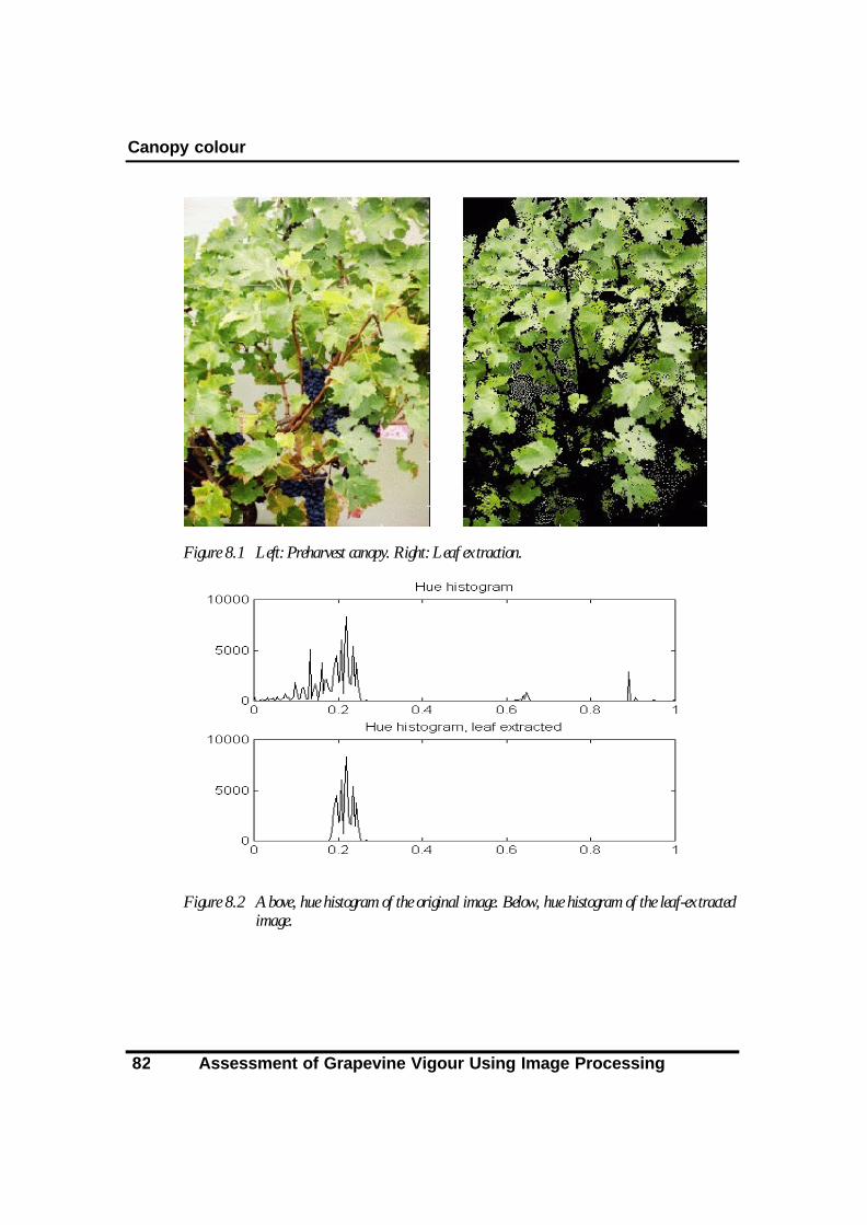
Canopy colour


Figure 8.1 Left: Preharvest canopy. Right: Leaf extraction.

Figure 8.2 Above, hue histogram of the original image. Below, hue histogram of the leaf-extracted image.

Canopy colour


8.2 Colour constancy When using colours to make decisions, it is important that the conditions under which the images are captured do not affect the outcome, e.g. the result should be the same regardless of whether it is a sunny or cloudy day. Therefore we seek an image capture technique that enables classification of its colour content.

Achieving colour constancy is very difficult. In [20] it was shown that current machine colour constancy algorithms are inadequate for colour-based object recognition. That research used a colour histogram to index and recognize different objects, but here the emphasis will be on colour recognition rather than object recognition.

Other research [21] has supported our notion that colour constancy algorithms perform well when searching for a specific colour.

8.3 Colour and reflection In a camera, the sensor comprises red, green and blue channels. Sensor response can be described by [22],[23]

λλλλρλ

dESR ii )()()(∫= Equation 8.1

where ρi is the ith sensor response, Ri(λ) is the camera’s sensitivity function of the ith sensor, S(λ) is the spectral reflectance of the surface and E(λ) is the spectrum of the incident illumination.

The goal in colour constancy is to characterize the reflectance from the camera response. This presents a difficult problem since for a given sensor response, there are many possible E(λ) and S(λ) that could provide the same response.

8.4 Approaches Two different approaches can be used to compensate for the large shift in image colours recorded by the camera for different illuminations. The first is to include in the picture, a colour chart with known colour values and the second is to use algorithms that imitate the human perception of colours, independent of lighting.

A set of five images ( Figure 8.3) of a colour chart is used to evaluate the different methods. The images were captured under different lighting conditions, using a colour chart consisting of 12 colour fields.

Canopy colour


Figure 8.3 Top left: Image 1 reference image. Top middle: Image 2 outdoor sunny. Top right: Image 3 indoor. Lower left: Image 4 outdoor shade. Lower right: Image 5 outdoor shade.

All results are described in Section 8.8.

8.5 Controlled lighting If images are captured under the same lighting condition, there is no need for calibration. This can be achieved by capturing the images at the same place, using the same light source, e.g. in a photographic studio. To achieve this with growing canopies, sample leaves can be removed and taken to a studio for image capture.

Alternatively, a controlled environment could be achieved outdoors at night time using an artificial light source.

8.6 Colour references in the image

8.6.1 Direct comparison One simple solution to classifying leaf colour is use of a reference colour chart in the picture. Ideally the chart colours would be similar to those of the leaves. Hence, a limitation of this method is that either the colour chart needs to include a large number of colours, or leaf colour classification will be coarse. The method might also fail if the image has non-uniform lighting.

Canopy colour


8.6.2 Shading correction The colour chart can also be used to calibrate the image, such as by shading correction [14] in the three different channels. The relation below is the basis for shading correction.

)],([),( yxfsyxb xy= Equation 8.2

where b(x,y) is the pixel value in the uncorrected image and f(x,y) is the ‘real’ pixel value. sxy is called the shading-function.

If sxy is known it is possible to calculate )],([),( 1 yxbsyxf xy−= . sxy is often

approximated and calculated by using at least two pixels with known values.

BB

AA

fcbcfcbc

=+=+

][][

21

21 Equation 8.3

This gives the two coefficients c1 and c2 where c1 is multiplicative and c2 is additive. The corrected value ),(ˆ yxf can then be calculated by using

),(]),([),(ˆ21 yxfcyxbcyxf ≈+= Equation 8.4

When applying this correction to a colour image, a shading-function is calculated for each colour channel (RGB).

One image is selected to be a reference image and the others are calibrated and corrected from this reference.

The shading-function for a colour channel (e.g. red) is calculated by using the values of the red component in the reference image, in the black and red squares. The corresponding values are measured in the image to be corrected and (Equation 8.4) applied to convert the red colour channel. If any corrected value is greater than 1 or less than 0 they are set to the appropriate limit.

The result from the shading correction of the test images is shown in Figure 8.4.

Canopy colour


Figure 8.4 Reference image (top left) and test images after shading correction.

The differences in colour value, 222 )()()( bbggrr rrr −+−+− , between the reference image and the other images for each colour in the colour chart before and after correction are given in Table 8.1.

8.7 Coefficient rule algorithms The methods described below are all based on the coefficient rule or von Kries model, where the change in illumination colour or geometry is approximated by multiplication with a 3 × 3 diagonal matrix T.

=

bgr

Tcba

Equation 8.5

8.7.1 Normalized RGB Dependency due to lighting intensity can be simplified and explained by the following model. If (r,g,b) is the camera response under one intensity, the camera response under a different intensity will be (sr, sg, sb).

Normalized RGB is widely used to produce images that are independent of lighting. The most common form is:

[ ]

++++++=

BGRB

BGRG

BGRR

bgr ,,,, Equation 8.6

The result from this form of RGB normalization is shown in Figure 8.5.

Canopy colour


Other methods of normalizing the RGB to eliminate the effects of intensity include

the use of BRr /= or 222/ BGRRr ++= etc.

Figure 8.5 Reference image (top left) and test images after RGB normalization, using Equation 8.6.

8.7.2 Grey world Illumination colour dependency can also be explained by the following model. (r,g,b ) is the camera response under one illumination colour and the response with a different illumination colour will be (αr, βg, γb). To make the image independent of illumination colour, it is normalized by

),,(

∑∑∑N

ii

N

ii

N

ii b

Nb

g

Ng

r

Nr Equation 8.7

This is called grey world normalization. The result is shown in Figure 8.6.

Canopy colour


Figure 8.6 Reference image (top left) and test images after grey world normalization.

8.7.3 Comprehensive normalization In [24] a colour constancy method called comprehensive normalization is presented. It combines features from the normalized RGB and grey world methods.

First, the pixels are normalized according to the RGB normalization in Equation 8.6 to remove dependence on lighting geometry. Then, the R, G and B colour channels are normalized to remove dependence on illumination colour, according to Equation 8.8, where (r1, g1, b1) and (r2, g2, b2) denote the camera response to two scene points viewed under one colour of light.

)2

,2

,2

(),2

,2

,2

(21

2

21

2

21

2

21

1

21

1

21

1

bbb

ggg

rrr

bbb

ggg

rrr

++++++ Equation 8.8

This process is iterated until it converges, indicated by little or no change in colour with each iteration.

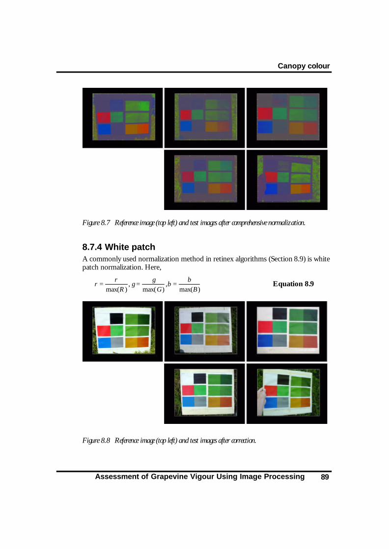
Canopy colour


Figure 8.7 Reference image (top left) and test images after comprehensive normalization.

8.7.4 White patch A commonly used normalization method in retinex algorithms (Section 8.9) is white patch normalization. Here,

)max(

,)max(

,)max( B

bb

Gg

gR

rr === Equation 8.9

Figure 8.8 Reference image (top left) and test images after correction.

Canopy colour


8.8 Results For every image and colour compensation method, the Euclidean distance of all 12 colour fields between the corrected image and the reference image is calculated. Recall that the Euclidean distance is the shortest distance between two points in space. The reference image is normalized in the same way as the other images.

Table 8.1 shows the mean and standard deviation of Euclidean distance for all algorithms and images.

Method mean std mean std mean std mean stdNone 0,218 0,108 0,375 0,157 0,222 0,080 0,189 0,086Shading 0,157 0,178 0,146 0,065 0,117 0,066 0,075 0,035NormRGB 0,117 0,125 0,169 0,113 0,168 0,113 0,069 0,044Greyworld 0,116 0,098 0,116 0,046 0,076 0,037 0,040 0,028Comcol 0,125 0,119 0,127 0,092 0,100 0,069 0,055 0,053White patch 0,223 0,100 0,208 0,063 0,125 0,063 0,155 0,054

Image 2 Image 3 Image 4 Image 5

Table 8.1 Mean and standard deviation of Euclidean distance between corrected and reference images.

In

Table 8.1, the mean of the difference between images decreases, indicating successful colour segmentation, for all algorithms on all images, except for white patch on image 2. The best performing algorithm is grey world. It is remarkable that shading correction does not consistently perform better than the other methods even though it uses references in the image.

Images captured in shadow provide the best correction result due to consistency in the lighting geometry, i.e. the light is the same all over the image.

Canopy colour


Mean

0

0,1

0,2

0,3

0,4

2 3 4 5

Image

NoneShadingNormRGBGreyworldComcolWhite

Figure 8.9 Mean of Euclidean distance in colour fields between reference and test images.

The standard deviation in image 2 increases or is unchanged for all algorithms. One reason for this is that image 2 was captured in sunlight and has bright reflections in the right hand side. The colour fields with bright reflections are not significantly improved by correction.

Standard deviation

0

0,05

0,1

0,15

0,2

2 3 4 5

Image

NoneShadingNormRGBGreyworldComcolWhite

Figure 8.10 Standard deviation of Euclidean distance in colour fields between reference and test images.

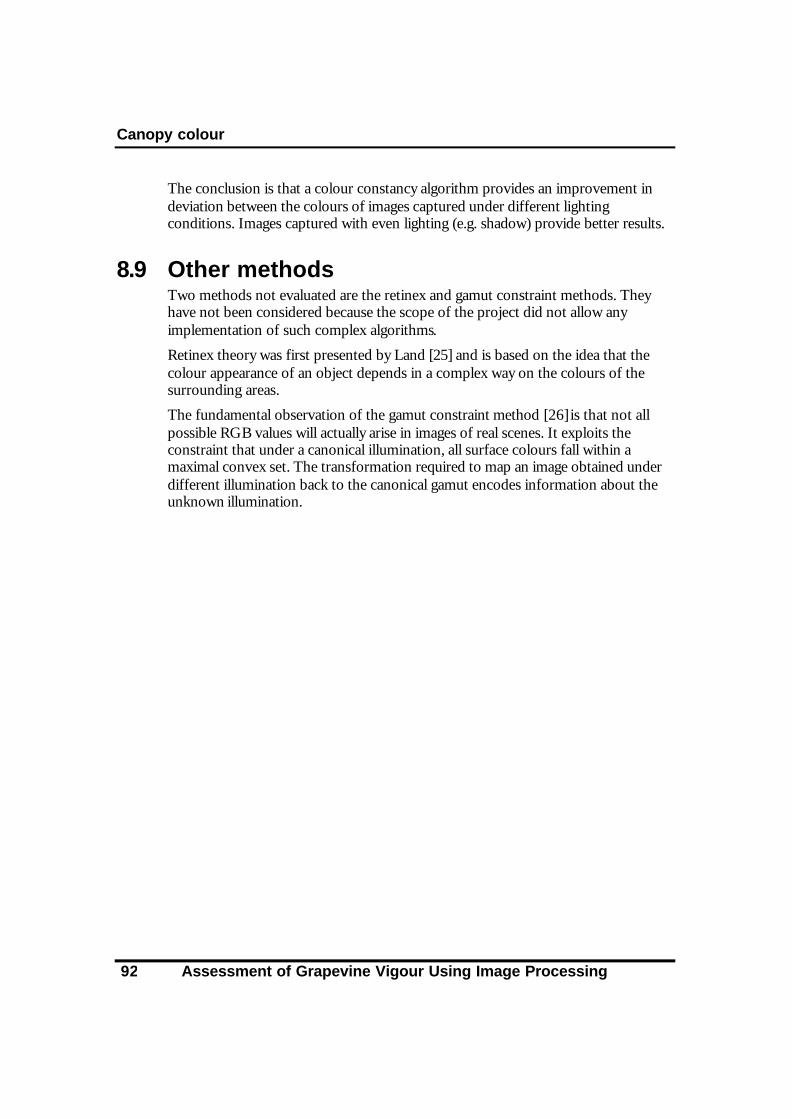
Canopy colour


The conclusion is that a colour constancy algorithm provides an improvement in deviation between the colours of images captured under different lighting conditions. Images captured with even lighting (e.g. shadow) provide better results.

8.9 Other methods Two methods not evaluated are the retinex and gamut constraint methods. They have not been considered because the scope of the project did not allow any implementation of such complex algorithms.

Retinex theory was first presented by Land [25] and is based on the idea that the colour appearance of an object depends in a complex way on the colours of the surrounding areas.

The fundamental observation of the gamut constraint method [26] is that not all possible RGB values will actually arise in images of real scenes. It exploits the constraint that under a canonical illumination, all surface colours fall within a maximal convex set. The transformation required to map an image obtained under different illumination back to the canonical gamut encodes information about the unknown illumination.

Other canopy assessments


99 Other canopy assessments This chapter contains a discussion on how assessment methods for other vine vigour characteristics explained in [2] could be achieved.

9.1 Canopy gaps This is the proportion of gaps in the canopy, but does not include the ‘holes’, which occur between spiky shoots at the edges of the canopy, leading to a difficulty in defining the valid canopy area.

One approach is to divide the image into smaller regions and require each of these regions containing more than a certain percent of leaves to belong to the canopy. The dividing line may be adjusted to achieve alignment with visual assessments.

Figure 9.1 Canopy gaps estimation. All regions in the canopy in the upper images are defined as canopy regions. In the canopy in the lower images the four middle regions are defined as canopy.

Other canopy assessments


Figure 9.1 shows an example on how this can be done. The images are divided into a number of slices, in this example 6. Each slice must have a certain percentage of leaves (i.e. white area) to be valid, in this example 40 %. The invalid slices are shaded. The thick canopy has a gap percentage of 22 % within the valid area, while the thin canopy has 32 %. The PQ (Section 7.5) gives the following results for the same regions: thick canopy 12.5 % and thin canopy 23 %. One reason for the deviation between the methods is that the PQ lacks resolution and does not count all gaps.

9.2 Fruit exposure This is the ratio between fruit exposed to the sun and the total quantity of fruit. The ratio would be difficult to estimate through a single image of the canopy since fruit that is not exposed on one side of the canopy may be exposed on the other side. The total amount of fruit has also to be approximated since it will not be visible on an image. However, by knowing the average size of a fruit cluster it should be possible to compare the exposed quantity of fruit to an approximation of total fruit quantity, achieved by counting all clusters that are at least partly visible and multiplying this figure with the average cluster size. This procedure would not account for the few fully obscured clusters.

9.3 Yield estimation Fruit extraction (Section 5.4) can be used to estimate the yield. After desuckering, where the leaves covering the fruit are removed, most of the fruit is visible, so a reasonable estimation can be expected.

9.4 Shoot length This is the average shoot length counted in nodes. It is expected that shoot length would be easy to calculate as long as the shoots are growing vertically and the relationship between metric shoot length and node shoot length is known.

If the camera is calibrated (Section 3.3.10), the shoot length can be translated from the number of pixels to a length unit, using projection calculations (Equation 3.1).

A vine assessment system


1100 A vine assessment system In this chapter we summarize the results from previous chapters and discuss how these could be used in a practical situation. Known difficulties and suggestions for future development are also discussed.

10.1 Results In Section 4.5.1 we demonstrated the procedure of mosaicing images to create one image of a whole row of vines. This image can be divided into vine bays or single vines by the techniques shown in Chapter 5 to identify posts and trunks. Hence, it is possible to collect data for entire rows, and the analysed data could be grouped or measured by row, bay or single vine.

10.1.1 Shoot counting As concluded in Chapter 6, shoot counting using image processing gives best accuracy if carried out at an early stage of growth. As soon as possible after all buds have burst and the leaves are still very small is the most appropriate time. If the image capture and counting is carried out later, the accuracy is lower and the ad hoc algorithms more complex and time consuming. Such algorithms have only been partly implemented in this project.

10.1.2 Canopy assessment In Chapter 7, different methods to estimate canopy density were shown. One method, stereo v ision, measures the actual depth of the canopy, whereas other methods use canopy features to estimate the canopy density.

When using the stereo method, the most accurate result is achieved by using two cameras. However, it is possible to calculate the depth using only one camera and use a horizontal displacement. The critical part with monocular stereo is the uncertainty of the distance between the images. One solution is to use parts of the image with a known distance to the camera to calibrate this separation. As an example, the intermediate posts along the rows could be used as reference objects, assuming that the camera can be kept at the same distance from the row.

Stereo image processing requires considerable computation time. However there are commercially available systems that can handle 320 × 240 pixels in real-time 30 Hz [27]. All methods have shown to give adequate results with a resolution of 320 × 240 pixels and 256 colours.

A vine assessment system


10.2 Proposed system Image capturing with a video camera has proved to be a suitable technique. The physical appearance of a vineyard with the grapevines in rows makes it easy to record a whole row at a time with the camera mounted on a vehicle. The camera could be attached on an arm so that it points back towards the vehicle from the other side of the vine, since this enables an image background to be attached to the vehicle. The distance from the camera to the vine should be 1 - 1.5 m with 35 mm focal length when capturing the canopy and 0.5 m when capturing shoots. The most suitable background is magenta since it is the complementary colour of green and therefore easily removed.

One concern with a video camera is the large amount of data that has to be processed. With a picture rate of 50 pictures per second and a resolution of 320 × 240 pixels and 256 colours, this will result in 30 MB data per minute. If monocular stereo is used it should be approximately 0.06 m between the images. This gives a horizontal velocity for the camera of 3 m/s and 30 MB data per 180 m, i.e. 17 MB per 100 m.

Most of this data is redundant and image sampling, based on the velocity of the vehicle, should be performed early to reduce image processing workload.

10.3 Major problems/known difficulties None of the methods have been tested on a larger set of test images and the correlation with manual methods is therefore uncertain.

The variation of the lighting conditions when images are captured is a major problem for calibration. It is difficult to make the methods work on images captured on different occasions without calibration. There are colour constancy algorithms to solve this problem but they do not work in all cases. As far as possible the images should be captured under the same lightning conditions and direct sunlight should be avoided.

10.4 Future development Since completing the experimental work and algorithm development described here, Lincoln Ventures had continued development of some of the methods described in the report. The performance of the algorithms and their correlation with manual methods were investigated using larger quantities of data. So far canopy density estimates using the intensity method (Section 7.4) were combined with a method that counts leaf edges. This correlates very well with the PQ method.

References


1111 References [1] Crossen T. Venture into viticulture. An introduction to the principles and

practices of viticulture. ISBN 0 7306 6635 2, 1997.

[2] Smart R. E. & Robinson M. Sunlight into wine. ISBN 1 8751 3010 1, 1991.

[3] Smith L. Precision management of vineyards using GIS. Environmental Perspectives: Araia atu ki te Tumataohikura. A Publication of the Environmental Policy & Management Research Centre, (Eds. Holt, A. & N. R. Wheen.) 21:13-14, ISSN: 1172-4420. 1998. http://divcom.otago.ac.nz:800/epmrc/6-21.html

[4] Burdick H. E. Digital Imaging, Theory and Applications. McGraw-Hill, ISBN 0-07-913059-3. 1997.

[5] Russ J.C. The Image Processing Handbook. Third Edition. CRC Press and IEEE Press, ISBN 0 8493 2532 3. 1999.

[6] Bergquist U. Colour vision and hue for autonomous vehicle guidance. Master’s Thesis project in computer vision, University of Linköping, 1999. ftp://ftp.isy.liu.se/pub/bb/Masters/Ex2091.pdf

[7] Faugeras O. Three Dimensional Computer Vision, MIT Press 1993.

[8] http://www.dai.ed.ac.uk/CVonline/LOCAL_COPIES/OWENS/LECT11

[9] Westelius C-J. Focus of Attention and Gaze Control for Robot Vision, PhD Dissertation no. 379, May 5, 1995.

[10] Zhang Z. & Deriche R. & Faugeras O. & Luong Q. A robust technique for matching two uncalibrated images through the recovery of the unknown epipolar geometry. Artificial Intelligence, 78:87--119, 1995.

[11] Forsyth D. & Ponce J. Computer Vision: A Modern Approach, 3rd draft version, online manuscript, to be published by Prentice-Hall 2001.

[12] Heikkilä J. http://www.ee.oulu.fi/~jth/calibr/Calibration.html

References


[13] Toft P. The Radon Transform - Theory and Implementation, Ph.D. thesis. Department of Mathematical Modelling, Technical University of Denmark, June 1996.

[14] Danielsson P-E & Seger O. & Magnusson-Seger M. Bildbehandling 2000, kapitel 1 -7. Institutionen för systemteknik, Linköpings Universitet, 2000.

[15] Lovell B.C. & Mudalige P. Machine vision for colour classification of fruits. ISBN 0 4730 4947 3. 1997.

[16] Paruelo J. M. & Lauenroth W. K. Technical note: Estimating aboveground plant biomass using a photographic technique. Journal of Range Management. 53(2):190-193, 2000.

[17] Moravec H. P. Visual Mapping By A Robot Rover, in `Proc. of the 6th Int. Joint Conf. on AI', Vol. 1, pp. 598-600. 1979.

[18] Lang F. & Förstner W. Matching Techniques, 1995.

[19] Okutomi M. & Kanade T. A multiple-baseline stereo, in IEEE Trans. on Pattern Analysis and Machine Intelligence, vol. 15, no. 4, pp. 353-363, 1993.

[20] Funt B. V. & Barnard K. & Martin L. Is colour constancy good enough?, 5th European Conference on Computer Vision, pages 445-459. 1998.

[21] Kwei G. & Barnard K. & Funt B.V. Spotting colours, Proceedings Colour Image Science 2000, Univ. of Derby, Derby England, 2000.

[22] http://kybele.psych.cornell.edu/~edelman/Course/lightness/node16.html.

[23] Barnard K. Computational colour constancy: taking theory into practice, MSc thesis, Simon Fraser University, School of Computing, 1995.

[24] Finlayson G. D. & Schiele B. & Crowley J. L. Comprehensive Colour Image Normalization. ECCV (1) 1998: 475-490.

[25] Land E. H. & McCann J. J. Lightness and Retinex Theory, J. Opt. Soc. Am, 61:1-11, 1971.

[26] Finlayson G. D. & Hordley S. Selection for Gamut Mapping Colour Constancy, http://www.bmva.ac.uk/bmvc/1997/papers/107/graham3.html.

References


[27] http://www.ai.sri.com/software/SVS.

References


På svenska

Detta dokument hålls tillgängligt på Internet – eller dess framtida ersättare –under en längre tid från publiceringsdatum under förutsättning att inga extra-ordinära omständigheter uppstår.

Tillgång till dokumentet innebär tillstånd för var och en att läsa, ladda ner,skriva ut enstaka kopior för enskilt bruk och att använda det oförändrat för ick-ekommersiell forskning och för undervisning. Överföring av upphovsrätten viden senare tidpunkt kan inte upphäva detta tillstånd. All annan användning avdokumentet kräver upphovsmannens medgivande. För att garantera äktheten,säkerheten och tillgängligheten finns det lösningar av teknisk och administrativart.Upphovsmannens ideella rätt innefattar rätt att bli nämnd som upphovsman i denomfattning som god sed kräver vid användning av dokumentet på ovan beskrivnasätt samt skydd mot att dokumentet ändras eller presenteras i sådan form eller isådant sammanhang som är kränkande för upphovsmannens litterära eller konst-närliga anseende eller egenart.

För ytterligare information om Linköping University Electronic Press se för-lagets hemsidahttp://www.ep.liu.se/

In English

The publishers will keep this document online on the Internet - or its possiblereplacement - for a considerable time from the date of publication barring excep-tional circumstances.

The online availability of the document implies a permanent permission foranyone to read, to download, to print out single copies for your own use and touse it unchanged for any non-commercial research and educational purpose. Sub-sequent transfers of copyright cannot revoke this permission. All other uses ofthe document are conditional on the consent of the copyright owner. The pub-lisher has taken technical and administrative measures to assure authenticity,security and accessibility.

According to intellectual property law the author has the right to be men-tioned when his/her work is accessed as described above and to be protectedagainst infringement.

For additional information about the Linköping University Electronic Pressand its procedures for publication and for assurance of document integrity, pleaserefer to its WWW home page:http://www.ep.liu.se/

© [Författarens för- och efternamn]

assessment of grapevine vigour using image processing

Documents