assessment of design and properties for flowable...
TRANSCRIPT
ASSESSMENT OF DESIGN AND PROPERTIES FOR FLOWABLE FILL
USAGE IN HIGHWAY PAVEMENT CONSTRUCTION FOR CONDITIONS IN FLORIDA
By
WEBERT LOVENCIN
A DISSERTATION PRESENTED TO THE GRADUATE SCHOOL OF THE UNIVERSITY OF FLORIDA IN PARTIAL FULFILLMENT
OF THE REQUIREMENTS FOR THE DEGREE OF DOCTOR OF PHILOSOPHY
UNIVERSITY OF FLORIDA
2007

Copyright 2007
by
Webert Lovencin

I would like to dedicate this dissertation to my parents, my lovely wife, April Adrienne Raines-Lovencin, my sister, Natacha Egland, my nieces and nephews, and to the tax payers who help fund
the public education systems in the state of Florida.

iv
ACKNOWLEDGMENTS
I would like to acknowledge those individuals who were involved in the advance-
ment of this research and throughout my studies. First, I would like to express my most
sincere gratitude to Dr. Fazil T. Najafi, my advisor and supervisory committee chairman.
Dr. Najafi has been a mentor, a friend, and a continuous source of encouragement both
professionally and personally. I thank Dr. Mang Tia, the cochair of my committee, for
his valuable advice and suggestions throughout the research study and dissertation.
I would also like to thank the other members of my committee, Dr. Walter E.
Dukes, Dr. David J. Horhota, Mr. Timothy J. Ruelke, and Mr. Michael J. Bergin, for their
continued support, constructive comments, and recommendations during my tenure at the
University of Florida.
Many debts of gratitude go out to the folks at the Florida Department of Transpor-
tation State Materials Office (Physical Lab and Geotechnical Divisions) and District 2 –
Materials Office in Lake City, who assisted me with this research study. These
individuals include Richard Delorenzo, Craig Roberts, Terry Thomas, Tim Blanton, Mike
Davis, Glenn Johnson, Ben Watson, Willie Henderson, Chris Falade, Bobby Ivory, Scott
Clayton, and Daniel Langley.
I would also like to express my gratitude to Drs. Claude Villiers and Jonathan F.
Earle, and Mrs. Margie Williams for their continuous encouragement and support, as well
as Mrs. Candace J. Leggett for her immense patience and efficient editorial assistance
with writing this dissertation.

v
Finally, I want to specially thank my savior, God (Jehovah), my family in the
United States and abroad from where they have always conferred me their support and
for believing in me the way they do. But above all, I want to deeply thank my beloved
wife, April, for her immense love, indispensable help and patience. April has been the
sole person responsible for my achieving this goal. She has been the wall containing my
worry, my best critic, and my greatest supporter.

vi
TABLE OF CONTENTS page
ACKNOWLEDGMENTS ................................................................................................. iv
LIST OF TABLES...............................................................................................................x
LIST OF FIGURES .......................................................................................................... xii
ABSTRACT.................................................................................................................... xvii
CHAPTER
1 INTRODUCTION ........................................................................................................1
1.1 Background............................................................................................................1 1.2 Problem Statement.................................................................................................2
1.2.1 Strength........................................................................................................2 1.2.2 Shrinkage.....................................................................................................3
1.3 Hypothesis .............................................................................................................5 1.4 Objectives ..............................................................................................................6 1.5 Scope......................................................................................................................6 1.6 Importance of Research .........................................................................................6 1.7 Research Approach................................................................................................7 1.8 Outline of the Dissertation.....................................................................................9
2 LITERATURE REVIEW ...........................................................................................10
2.1 Introduction..........................................................................................................10 2.2 Flowable Fill Technology....................................................................................10
2.2.1 Introduction ...............................................................................................10 2.2.2 Types of Flowable Fill...............................................................................11 2.2.3 Advantages of Using Controlled Low Strength Material (CLSM) ...........11 2.2.4 Engineering Characteristics of CLSM.......................................................13 2.2.5 Uses of Flowable Fill.................................................................................13 2.2.6 Delivery and Placement of Flowable Fill ..................................................14 2.2.7 Limits.........................................................................................................15
2.3 Specifications, Test Methods, and Practices........................................................15 2.3.1 Introduction ...............................................................................................15 2.3.2 ASTM Standard Test Methods..................................................................17

vii
2.3.2.1 Standard Test Method for Preparation and Testing of CLSM Test Cylinders (ASTM D 4832-02) ..............................................17
2.3.2.2 Standard Practice for Sampling Freshly Mixed CLSM (ASTM D 5971-96) ..................................................................................18
2.3.2.3 Standard Test Method for Unit Weight, Yield, Cement Content and Air Content (Gravimetric) of CLSM (ASTM D 6023-96) ................18
2.3.2.4 Standard Test Method for Ball Drop on CLSM to Determine Suitability for Load Application (ASTM D 6024-96)..............................19
2.3.2.5 Standard Test Method for Flow Consistency of CLSM (ASTM D 6103-96) ..................................................................................20
2.3.3 Other Currently Used and Proposed Test Methods...................................20 2.3.4 Specifications by the State Departments of Transportation ......................22 2.3.5 Use of Flowable Fill in the State of Florida ..............................................24
2.3.5.1 Material Specifications (Section 121-2)..........................................24 2.3.5.2 Construction Requirements and Acceptance (Section
121-5, 121-6) ............................................................................................25 2.3.5.3 Guideline for Construction Requirements and Acceptance
(Section 121-5, 121-6) ..............................................................................25 2.4 Early Set and Strength Development...................................................................26
2.4.1 Introduction ...............................................................................................26 2.4.2 Behavior of Slurries...................................................................................26 2.4.3 Early Hydration of Cement Particles.........................................................27 2.4.4 Influence of Water to the Hydration of Cement ........................................28 2.4.5 Effects of Set Accelerator on Hydration of Cement..................................29 2.4.6 Set Time.....................................................................................................29 2.4.7 Strength Development ...............................................................................30 2.4.8 Use of Mineral Admixture (Fly Ash and Granulated Ground Blast
Furnace Slag) in Flowable Fill.........................................................................31 2.4.8.1 Fly ash .............................................................................................31
2.4.8.2 Slag .........................................................................................................34 2.4.8.3 Difference between fly ash and slag................................................36 2.4.8.4 Specific applications .......................................................................36 2.4.8.5 Mixture proportioning/mixture compliance ....................................36
2.4.9 Effect of Moisture on Strength ..................................................................37 2.5 Strength Prediction Models .................................................................................38
2.5.1 Introduction ...............................................................................................38 2.5.2 Hamilton County–Removability Index .....................................................38 2.5.3 Bhat’s Study ..............................................................................................39 2.5.4 NCHRP–Study ..........................................................................................40
2.6 FDOT/UF Flowable Fill Study............................................................................42
3 MATERIALS AND LABORATORY EXPERIMENTAL PROGRAM...................44
3.1 Introduction..........................................................................................................44 3.2 Experimental Design ...........................................................................................44
3.2.1 Rationale for Selecting Mixture Parameters..............................................44 3.2.2 Mixture Proportioning ...............................................................................46

viii
3.2.3 Specimen Sample Collection per Batch Mix.............................................49 3.2.4 Specimen Molds ........................................................................................49 3.2.5 Fabrication of Flowable Fill Specimens....................................................50
3.2.5.1 Preparation of molds .......................................................................50 3.2.5.2 Mixing of flowable fill ....................................................................50 3.2.5.3 Casting of flowable fill....................................................................53
3.3 Limerock Bearing Ratio Test (Florida Test Method 5-515)................................55 3.4 Compressive Strength Test ..................................................................................60 3.5 Proctor Penetrometer Test ...................................................................................64 3.6 Drying Oven ........................................................................................................65 3.7 Drying Shrinkage of Flowable Fill Mixtures.......................................................65
3.7.1 Method 1....................................................................................................66 3.7.2 Method 2....................................................................................................69 3.7.3 Method 3....................................................................................................70
3.8 Materials ..............................................................................................................71 3.8.1 Cement.......................................................................................................71 3.8.2 Fly Ash ......................................................................................................72 3.8.3 Blast Furnace Slag.....................................................................................72 3.8.4 Aggregates.................................................................................................73
3.8.4.1 Aggregate gradation ........................................................................74 3.8.4.2 Physical properties, absorption and moisture content .....................76 3.8.4.3 Storage of fine aggregates ...............................................................77
3.8.5 Admixtures ................................................................................................78 3.8.6 Water .........................................................................................................78
4 LABORATORY RESULTS AND DISCUSSIONS ..................................................79
4.1 Introduction..........................................................................................................79 4.2 Laboratory Results...............................................................................................79
4.2.1 Limerock Bearing Ratio (LBR).................................................................79 4.2.2 Compressive Strength (psi) .......................................................................79 4.2.3 Volume Change .........................................................................................84 4.2.4 Proctor Penetrometer Setting Strength (psi)..............................................85 4.2.5 Strength Gained Between 28 and 56 Days ................................................91 4.2.6 LBR Oven Sample Results........................................................................92
4.3 Factors Affecting Strength...................................................................................96 4.3.1 Water-to-Cement (w/c) Ratio ....................................................................96 4.3.2 Cement Content .........................................................................................98 4.3.3 Effect of Air Content on Strength ...........................................................100 4.3.4 Effect of Mineral Admixtures (Fly Ash and Blast Furnace Slag) on
Strength ..........................................................................................................101 4.4 Comparison of Mix Using Type I/II Cement vs. Type I Cement ......................102 4.5 Drying Shrinkage (Volume Change) .................................................................105 4.6 Interpretation of Plastic Test Results.................................................................108

ix
5 STATISTICAL ANALYSIS ....................................................................................111
5.1 Introduction........................................................................................................111 5.2 Statistical Model Derivation ..............................................................................111 5.3 Accelerating Strength Testing ...........................................................................118
5.3.1 Background..............................................................................................118 5.3.2 Accelerated Curing..................................................................................119 5.3.3 Analysis ...................................................................................................119 5.3.4 Confidence Band for Regression Line ....................................................124 5.3.5 Estimate of Later Strength.......................................................................124 5.3.6 Analysis on Other Samples .....................................................................125
5.4 Model Validation and Evaluation of Accuracy .................................................128 5.4.1 Varying Strength Prediction Models for Trend.......................................128 5.4.2 Comparison of Strength Prediction Models ............................................145 5.4.3 Mixture Design Examples to Validate Models .......................................150
5.5 Summary of Model Equations and Limitations.................................................157
6 SUMMARY, CONCLUSIONS AND RECOMMENDATIONS ............................164
6.1 Summary............................................................................................................164 6.2 Conclusions........................................................................................................166 6.3 Recommendations..............................................................................................167
APPENDIX
A FLOWABLE FILL STUDY BATCH MIX DESIGN MATRIX.............................169
B LBR AND COMPRESSIVE STRENGTH DATA OBTAINED IN THE LABORATORY.......................................................................................................185
C ANALYSIS OF VARIANCE (ANOVA), PARAMETERS, AND STANDARD ERROR FOR MODELS....................................................................200
D ESTIMATED 28- AND 56-DAY STRENGTH.......................................................215
LIST OF REFERENCES.................................................................................................252
BIOGRAPHICAL SKETCH ...........................................................................................257

x
LIST OF TABLES
Table page 2-1. Current ASTM standards on controlled low strength material (CLSM) ...................16
2-2. States surveyed and their specification on flowable fill ............................................22
2-3. Specified acceptance strengths and ages ...................................................................23
2-4. Suggested mixture proportions, lb/yd3 .....................................................................23
2-5. FDOT materials specification requirements..............................................................24
2-6. FDOT flowable fill mix design .................................................................................25
2-7. Removability modulus (RE) ......................................................................................39
3-1. Mixture parameters....................................................................................................45
3-2. Summary of sample specimens collected per mix.....................................................49
3-3. Properties of fresh flowable fill (Experiment 1)........................................................56
3-4. Properties of fresh flowable fill (Experiment 2)........................................................57
3-5. Specifications for LBR test equipment......................................................................59
3-6. Chemical composition of cement used......................................................................71
3-7. Physical characteristics of cement.............................................................................72
3-8. Chemical and physical analyses of fly ash ................................................................73
3-9. Chemical and physical analyses of blast furnace slag...............................................73
3-10. Fine aggregate location source ................................................................................74
3-11. ASTM C33-02A and FDOT specifications for fine aggregate gradation ...............75
3-12. Physical properties of fine aggregates (silica sand).................................................76
4-1. LBR strength results for Experiment #1....................................................................80

xi
4-2. LBR strength results for Experiment #2....................................................................81
4-3. Compressive strength results for Experiment #1.......................................................82
4-4. Compressive strength results for Experiment #2.......................................................83
4-5. Volume change results for Experiment #1 ................................................................86
4-6. Volume change results for Experiment #2 ................................................................87
4-7. Mix proportions and proctor penetrometer results for Experiment #1......................88
4-9. Two-day oven LBR strength results for Experiment #1............................................93
4-10. Two-day oven LBR strength results for Experiment #2..........................................94
4-11. Comparison of mixture components and their influence on accelerated 2-day oven and 28-day LBR strength ......................................................................95
4-12. Comparison of mixture components and their influence on percent volume change........................................................................................................106
5-1. Standard error of regression coefficients for equations relating mixture constituents to LBR, compressive strength and percent volume change ...............116
5-2. Estimation of confidence interval for 28-day strength ............................................122
5-3. Summary of regression equations for accelerated (oven) 28-day and 56-day LBR strength .......................................................................................127
5-4. NCHRP’s CLSM mixture proportions and fresh properties [38]............................146
5-5. Comparison of the NCHRP measured and predicted 28-day strength for air-entrained mixtures strength prediction model.............................................147
5-6. Comparison of estimated 28-day compressive strength ..........................................149
5-7. Summary of materials required for validation mixtures..........................................154
5-8. Summary of plastic properties of validation mixture models..................................155
5-9. Comparison of estimated and experimental results for batch mixes 1v through 6v .....................................................................................158
5-10. Comparison of estimated and experimental results for batch mixes 7v through 11v ...................................................................................159
5-11. Summary of recommended strength prediction equations listed with variables and range.........................................................................................162

xii
LIST OF FIGURES
Figure page 1-1. Laboratory task process ...............................................................................................8
2-1. Influence of water/cement (w/c) ratio on the setting of Portland cement paste ........28
2-2. Bhat’s strength prediction model...............................................................................40
3-1. Concrete mixer used in study ....................................................................................51
3-2. Pressure meter test for air content .............................................................................52
3-3. Cast flowable fill in LBR samples.............................................................................53
3-4. Cast flowable fill in 4-in. × 8-in. (compressive strength) samples............................54
3-5. Cast flowable fill in 6-in. × 12-in. (volume change) samples ...................................54
3-6. Cross section of seated LBR penetration piston [30] ................................................58
3-7. LBR machine.............................................................................................................59
3-8. Graph example showing typical load penetration curve that requires no correction...............................................................................................61
3-9. Graph example showing correction of typical load penetration curve for small surface irregularities........................................................................62
3-10. Typical set-up for compressive strength test ...........................................................63
3-11. Typical proctor penetrometer ..................................................................................64
3-12. Test set-up for measuring shrinkage using LVDTs.................................................68
3-13. Schematic of test set-up for measuring shrinkage using LVDTs ............................68
3-14. Three-dial gauge reading method ...........................................................................69
3-15. Dial gauge shrinkage reading being taken...............................................................70
3-16. Gradation of fine aggregates–ASTM specs.............................................................75

xiii
3-17. Gradation of fine aggregates–FDOT specs .............................................................76
3-18. Storage and removal of fine aggregates ..................................................................77
4-1. Load deformation responses for batch mix #4, at 3-, 28- and 56-day duration.........84
4-2. Percent increase in 56-day strength as compared to 28-day strength (LBR) ............91
4-3. Percent increase in 56-day strength as compared to 28-day strength (psi) ...............92
4-4. Relationship between 28-day bearing strength (LBR) and w/c ratio at 7.5% design air content .....................................................................................................96
4-5. Relationship between 28-day bearing strength (LBR) and w/c ratio at 17.5% design air content .......................................................................96
4-6. Relationship between 28-day compressive strength (psi) and w/c ratio at 7.5% design air content .........................................................................97
4-7. Relationship between 28-day compressive strength (psi) and w/c ratio at 17.5% design air content .......................................................................97
4-8. Relationship between 28-day bearing strength (LBR) and cement content at 7.5% design air content ...............................................................98
4-9. Relationship between 28-day bearing strength (LBR) and cement content at 17.5% design air content .............................................................98
4-10. Relationship between 28-day compressive strength (psi) and cement content at 7.5% design air content ...............................................................99
4-11. Relationship between 28-day compressive strength (psi) and cement content at 17.5% design air content .............................................................99
4-12. Relationship between 28-day LBR strength and cement content............................99
4-13. Relationship between 28-day compressive strength (psi) and cement content .....100
4-14. Effect of mineral admixtures on 28-day LBR strength .........................................101
4-15. Effect of mineral admixtures on 56-day LBR strength .........................................102
4-16. Compressive strength (psi) of Type I/II vs. Type I cement for BM15..................103
4-17. LBR strength of Type I/II vs. Type I cement for BM15 .......................................103
4-18. Compressive strength (psi) of Type I/II vs. Type I cement for BM 25.................103
4-19. LBR strength of Type I/II vs. Type I cement for BM 25 ......................................104

xiv
4-20. Compressive strength (psi) of Type I/II vs. Type I cement for BM 48.................104
4-21. LBR strength of Type I/II vs. Type I cement for BM 48 ......................................104
4-22. Compressive strength (psi) of Type I/II vs. Type I cement for BM 54.................105
4-23. LBR strength of Type I/II vs. Type I cement for BM 54 ......................................105
4-24. Effect of w/c ratio on volume change....................................................................107
4-25. Effect of cement content on volume change .........................................................107
4-26. Effect of mineral admixtures on volume change...................................................108
4-27. Flow diameter vs. sand-to-water ratio ...................................................................110
5-1. Residuals versus fitted values plot (28-day LBR) ...................................................116
5-2. Residuals versus fitted values plot (28-day psi) ......................................................117
5-3. Residuals versus fitted values plot (% volume change) ..........................................117
5-4. Accelerated curing vs. 28-day normal curing strength............................................123
5-5. Accelerated curing vs. 28-day normal curing strength for all mixtures ..................126
5-6. Accelerated curing vs. 56-day normal curing strength for all mixtures ..................126
5-7. Estimated 28-day LBR strength vs. cement content at fixed air (15%) and fixed 0% mineral admixture ............................................................................130
5-8. Estimated 56-day LBR strength vs. cement content at fixed air (15%) and fixed 0% mineral admixture ............................................................................130
5-9. Estimated 28-day compressive strength vs. cement content at fixed air (15%) and fixed 0% mineral admixture...................................................131
5-10. Estimated 28-day compressive strength vs. cement content at fixed air (15%) and fixed 0% mineral admixture...................................................131
5-11. Estimated volume change vs. cement content at fixed air (15%) and fixed 0% mineral admixture ...................................................................................132
5-12. Estimated 28-day LBR strength vs. w/c ratio at fixed air (15%) and fixed 0% mineral admixture ...................................................................................132
5-13. Estimated 56-day LBR strength vs. w/c ratio at fixed air (15%) and fixed 0% mineral admixture ...................................................................................133
xv
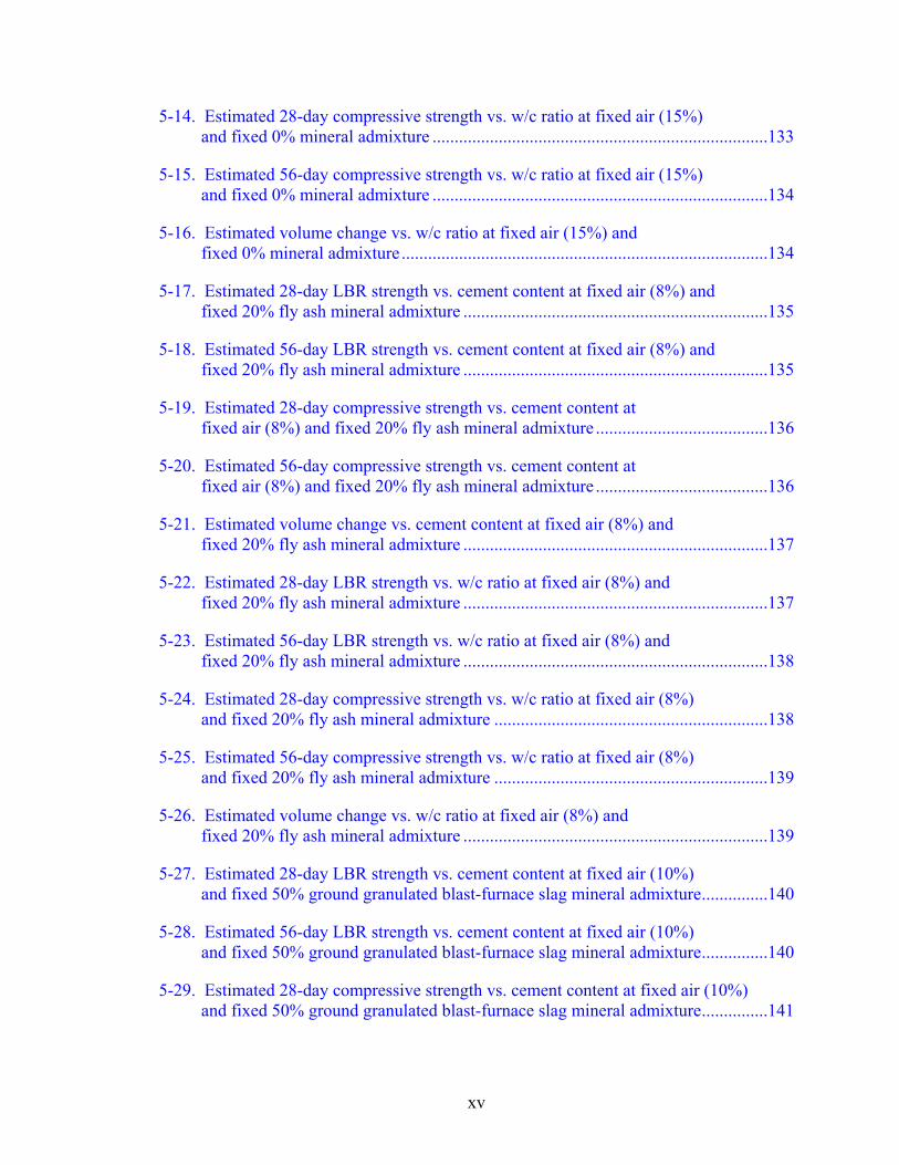
5-14. Estimated 28-day compressive strength vs. w/c ratio at fixed air (15%) and fixed 0% mineral admixture ............................................................................133
5-15. Estimated 56-day compressive strength vs. w/c ratio at fixed air (15%) and fixed 0% mineral admixture ............................................................................134
5-16. Estimated volume change vs. w/c ratio at fixed air (15%) and fixed 0% mineral admixture ...................................................................................134
5-17. Estimated 28-day LBR strength vs. cement content at fixed air (8%) and fixed 20% fly ash mineral admixture .....................................................................135
5-18. Estimated 56-day LBR strength vs. cement content at fixed air (8%) and fixed 20% fly ash mineral admixture .....................................................................135
5-19. Estimated 28-day compressive strength vs. cement content at fixed air (8%) and fixed 20% fly ash mineral admixture .......................................136
5-20. Estimated 56-day compressive strength vs. cement content at fixed air (8%) and fixed 20% fly ash mineral admixture .......................................136
5-21. Estimated volume change vs. cement content at fixed air (8%) and fixed 20% fly ash mineral admixture .....................................................................137
5-22. Estimated 28-day LBR strength vs. w/c ratio at fixed air (8%) and fixed 20% fly ash mineral admixture .....................................................................137
5-23. Estimated 56-day LBR strength vs. w/c ratio at fixed air (8%) and fixed 20% fly ash mineral admixture .....................................................................138
5-24. Estimated 28-day compressive strength vs. w/c ratio at fixed air (8%) and fixed 20% fly ash mineral admixture ..............................................................138
5-25. Estimated 56-day compressive strength vs. w/c ratio at fixed air (8%) and fixed 20% fly ash mineral admixture ..............................................................139
5-26. Estimated volume change vs. w/c ratio at fixed air (8%) and fixed 20% fly ash mineral admixture .....................................................................139
5-27. Estimated 28-day LBR strength vs. cement content at fixed air (10%) and fixed 50% ground granulated blast-furnace slag mineral admixture...............140
5-28. Estimated 56-day LBR strength vs. cement content at fixed air (10%) and fixed 50% ground granulated blast-furnace slag mineral admixture...............140
5-29. Estimated 28-day compressive strength vs. cement content at fixed air (10%) and fixed 50% ground granulated blast-furnace slag mineral admixture...............141

xvi
5-30. Estimated 56-day compressive strength vs. cement content at fixed air (10%) and fixed 50% ground granulated blast-furnace slag mineral admixture...............141
5-31. Estimated volume change vs. cement content at fixed air (10%) and fixed 50% ground granulated blast-furnace slag mineral admixture .....................142
5-32. Estimated 28-day LBR strength vs. w/c ratio at fixed air (10%) and fixed 50% ground granulated blast-furnace slag mineral admixture .....................142
5-33. Estimated 56-day LBR strength vs. w/c ratio at fixed air (10%) and fixed 50% ground granulated blast-furnace slag mineral admixture .....................143
5-34. Estimated 28-day compressive strength vs. w/c ratio at fixed air (10%) and fixed 50% ground granulated blast-furnace slag mineral admixture .....................143
5-35. Estimated 56-day compressive strength vs. w/c ratio at fixed air (10%) and fixed 50% ground granulated blast-furnace slag mineral admixture .....................144
5-36. Estimated volume change vs. w/c ratio at fixed air (10%) and fixed 50% ground granulated blast-furnace slag mineral admixture...............................144
5-37. Comparison of measured and predicted 28-days strength.....................................147
5-38. Comparison of estimated 28-day compressive strength for Bhat, NCHRP, and dissertation models...........................................................................150
5-39. Comparison of estimated 28-day compressive strength for NCHRP and dissertation models ..........................................................................................150
5-40. Comparison of measured and predicted 28-day LBR strength of validation mixtures of model...................................................................................................160
5-41. Comparison of measured and predicted 28-day compressive strength of validation mixtures of model..................................................................................160
5-42. Comparison of measured and predicted 28-day (oven) LBR strength of validation mixtures of model..................................................................................161

xvii
Abstract of Dissertation Presented to the Graduate School of the University of Florida in Partial Fulfillment of the Requirements for the Degree of Doctor of Philosophy
ASSESSMENT OF DESIGN AND PROPERTIES FOR FLOWABLE FILL USAGE IN HIGHWAY PAVEMENT CONSTRUCTION
FOR CONDITIONS IN FLORIDA
By
Webert Lovencin
May 2007
Chair: Fazil T. Najafi Cochair: Mang Tia Major Department: Civil and Coastal Engineering
Flowable fill, also known as controlled low-strength material (CLSM), is a self
compacting cementitious material primarily used as a backfill in lieu of compacted soil.
Flowable fill is an extremely versatile construction material that has been used in a wide
variety of applications. There are two types of flowable fill, excavatable and
nonexcavatable. An excavatable flowable fill mixture is considered excavatable when
the 28-day compressive strength is 100 psi. Nonexcavatable mixtures are mixes in which
the minimum design strength is at 125 psi or greater. The ability to control and predict
the strength and volume change (shrinkage) is an important aspect to consider when
designing a flowable fill mixture. Various studies have been conducted to better
understand and predict quality control measures such as the strength and the occurrence
of shrinkage in flowable fill.
xviii
The aim of this research was to vary components of excavatable flowable fill
mixtures. A 4 × 3 × 2 × 3 factorial design (i.e., 4 levels of cement, 3 levels of mineral
admixtures, 2 levels of air content, and 3 levels of water/cement ratio) was applied to
evaluate the compressive strength, limerock bearing ratio (LBR) strength, and shrinkage.
With this study’s objective in mind, a total of 58 mixtures were selected from the
factorial design matrix and batched in a laboratory. The strength of the mixtures was
evaluated at 6 hours, 1 day, 2 days oven cured, 3 days, 28 days and 56 days.
Mathematical models were developed to predict the LBR, compressive strength,
and volume change. An accelerated curing method, along with prediction models, was
developed to help estimate long-term strength of flowable fill. Based on the performance
of the statistical analysis, it was found that the models developed from this study
provided good correlations for estimating strength and volume change of excavatable
flowable fill mixture. Though the models were found to provide good correlations, the
formula developed for estimating the volume change was found to be unacceptable for
design application. This study provides a rational method for engineers to utilize when
designing flowable fill mixture.

1
CHAPTER 1 INTRODUCTION
1.1 Background
The construction industry searches for the most cost and time efficient means for
completing its projects. Many of these projects include cutting and backfilling trenches
for structure and drainage pipe installation. Often cutting and backfilling trenches
disrupts major traffic arteries. Standard practice for backfilling trenches includes soil
being placed in 6-inch lifts and compacted until a minimum density threshold is achieved.
The soil tests required to set and verify the density threshold in the field require several
days to complete. To help in this matter, newer forms of construction material have been
introduced. The most common is called controlled low strength material (CLSM), also
known as flowable fill. The use of flowable fill negates the need for placing the 6-inch
lifts and eliminates the need for practically all tests, excluding a simple in-place soil test.
Flowable fill is an extremely versatile construction material that has been used in a
wide variety of applications. Among the many successful applications of flowable fill are
slurried backfill for walls, culverts, pipe trenches, bridge abutments and retaining walls;
backfill for abandoned underground structures (including mines) or tanks; and floating
slab foundation for lightweight structures [1,2]. Flowable fill offers a number of
advantages over conventional earthfill materials that require controlled compaction in
layers [2]. The advantages include ease of mixing and placement, the ability to flow into
hard-to-reach places, and the self-leveling characteristic of the fill.

2
1.2 Problem Statement
1.2.1 Strength
Flowable fill answers the need for a fill that allows prompt return to traffic flow,
does not settle, does not require vibration or other means of compaction, can be
excavated, is fast to place, and safer than other forms of fill. One requirement typically
encountered with flowable fill is the need to limit the maximum compressive strength [3].
This requirement is necessary in cases where future excavation may be required for
maintenance and repair of embedded utilities. To predict the long-term strength and the
excavatability of flowable fill using conventional excavating equipment, many
approaches are employed. One approach for predicting whether or not a flowable fill mix
is excavatable is to develop a correlation using its early age strength and long-term
strength. For example, a mixture exhibiting strength that is less than 100 psi would be
classified as being excavatable. Mixtures resulting in strengths higher than 100 psi would
be very difficult to excavate and would be termed nonexcavatable.
According to Digiola and Brenda [4], the proper control of strength in flowable fill
is an important criterion used to develop a mix design. Despite this known criterion, a
review of literature shows few studies published in proper control of strength in flowable
fill. In using flowable fill, not only is it required to meet minimal strengths to maintain
and provide suitable structural support, but the maximum strength development must also
be controlled to allow for future excavation. A study by Pons et al. [3] shows that in
1994, about 80% of the concrete producer market producing flowable fill carried the
understanding or expectation for excavatability. For these reasons, design strengths often
must be assigned a range of strengths from “minimally acceptable” to “maximum
allowable.”

3
Many state agencies specify acceptance strengths at a curing age of 28 days, while
others include 56-day strength in their specifications [5]. In some cases, the maximum
strengths are listed to enable excavation for a later date. Some state agencies, however,
list the target strengths instead of maximum strengths which causes some concrete plants
to produce flowable fill mixes with minimum strength, as they would normally for
Portland cement concrete. In general, the desired strength is the maximum hardness that
can be excavated at a later date using conventional excavating equipment. The existing
Florida Department of Transportation (FDOT) flowable fill specification requires field
tests to verify that a minimum penetration resistance is achieved.
Flowable fill mixtures are usually designed on the basis of compressive strength
development. Little information is available in which the terminology used for
describing the strength of flowable fill is something other than compressive strength.
This method of describing the quality of flowable fill is conventional throughout the
ready mix industry. Because flowable fill is used as a backfill material similar to soil, a
suitable unit instead of compressive strength, such as limerock bearing ratio (LBR), is
needed to describe the in-place bearing strength of the flowable fill mixture. Making
such a change would alter the state-of-the-art for relating the quality of strength for
flowable fill mixtures.
1.2.2 Shrinkage
To understand why shrinkage occurs, one must first understand the materials in
flowable fill. Just as shrinkage occurs in concrete, it also occurs in flowable fill.
Cement, a key ingredient in flowable fill, when mixed with water forms a paste and a
chemical reaction called “hydration” occurs. The hardened cement paste is what binds all
the other ingredients together to create flowable fill.

4
During the process of hydration, tiny voids filled with water and air form in the
paste. The more porous the cement paste is in a mixture, the weaker the mixture. Studies
have shown that voids in concrete play a vital role in shrinkage. After pouring, concrete
will change volume as moisture levels change. In flowable fill this phenomenon also
takes place. Another condition playing a key role in concrete shrinkage is temperature.
Expansion and shrinkage due to changes in temperature can put stress on flowable fill,
resulting in cracks.
Studies have shown that high water/cement (w/c) ratio and high water content are
the two factors known to cause unwarranted drying-shrinkage in concrete. Although
flowable fill has a higher w/c ratio and higher water content than concrete, studies on
drying shrinkage have indicated that flowable fill exhibits shrinkage to a lesser extent
than concrete. Typical reports of linear-shrinkage values on flowable fill are in the range
of 0.002 to 0.05 percent (6). These values are similar to concrete with low drying
shrinkage. The shrinkage and expansion of flowable fill tend to continue varying
throughout testing. A study by Grandham et al. (7) found that the maximum shrinkage
and expansion values of flowable fill were generally less than the acceptable limit
established for concrete (7).
Since flowable fill is often placed underneath roadways as a road base, varying
volume change is an important attribute to investigate. In various parts of Florida
moisture is greatly abundant. Because this is so, when flowable fill is used in these areas,
it is affected, forcing the flowable fill volume to alter. From the volume change
activities, cracks are often created, leading to water seepage through the cracks causing

5
roadbed damage and deficiencies in the roadway. The final result may include pavement
depressions or pavement humps.
Various problems encountered while using flowable fill arise from the lack of
documented procedures to measure or determine long-term strength for future excava-
tion. Some areas that need further investigation and documentation are as follows:
• A practical method for designing flowable fill mixtures.
• A thorough investigation of the effects of shrinkage in flowable fill.
• A developed flowable fill design method that utilizes commonly used units for describing the strength of backfill materials, such as limerock bearing ratio (LBR) instead of compressive strength.
• A study identifying long-term performance of flowable fill, particularly how the plastic properties of flowable fill affect its long-term strength and excavatability.
It is critical that research be conducted at this time given there is a large number of
roadway construction, maintenance, and rehabilitation projects taking place throughout
Florida.
1.3 Hypothesis
Several factors in flowable fill are found to be similar to those identified in concrete
as a controlled measure for predicting strength. The factors include w/c ratio, cement
content, fly ash content, and plastic properties. The following hypothetical questions
may be asked: (1) Is it possible to get target strength (100 LBR) for flowable fill if
quantities of its mixture components are known? (2) If so, can varying the components of
flowable fill mix help target strength and shrinkage?
Laboratory experiments can be conducted to identify key components to help lay a
foundation for developing rational methods to approach development of flowable fill
mixture design for construction. In addition, models can be developed to employ known

6
component parameters to produce reliable results for predicting strength and field
performance (i.e., shrinkage) of flowable fill.
1.4 Objectives
The primary objectives of this research are as follows:
• Vary mixture components of flowable fill, to help predict strength using prediction models.
• Vary mixture components to predict shrinkage in flowable fill using a prediction model.
• Develop mix design procedures utilizing fine aggregate materials commonly used for flowable fill in the state of Florida.
• Identify setting behavior of flowable fill.
• Provide recommendations where warranted from findings.
1.5 Scope
This is a continuance of a preliminary study in which the key goal was to evaluate
the performance of flowable fill in pavement sections using accelerated and nonacceler-
ated mixtures. Using knowledge acquired from the findings of the preliminary study, the
scope of the current research will focus on developing strength prediction models that
incorporate flowable fill mix parameters. It is critical to vary known components (i.e., air
content, cementitious content, etc.) for establishing the framework and creating the
database to use for prediction models. Thus, this research will focus on the effects of the
following:
• strength in LBR for flowable fill mixtures; and • change in flowable fill volume due to shrinkage.
1.6 Importance of Research
The proper control of strength development in flowable fill applications is an
important criterion in developing a design mixture. Very few studies have been

7
published evaluating the long-term strength of flowable fill in LBR. This research will
help to develop mix design procedures for concrete producers using flowable fill and will
benefit the construction industry.
The volume changes due to shrinkage are of considerable importance. If the
amount of volume change in flowable fill due to shrinkage is derivable, producers will be
able to modify their mixes for obtaining optimal mixtures. Also, contractors can
compensate as necessary.
1.7 Research Approach
To meet the research objectives, this study was conducted utilizing the process
categorized as tasks provided below.
• Task 1 – Literature search: − Examine existing ideas, theories and results published about flowable fill
reviewing various properties affecting its mixtures − Review work done on concrete and geotechnical engineering practices − Review past and current flowable fill practices – materials, design mixes,
properties, and testing practices to measure performance. • Task 2 – Data collection:
− Prepare laboratory design mixtures − Design the experiment for laboratory mixtures
Use factorial design Vary mixture components (i.e., cement, fly ash/slag, and
water/cement ratio) Prepare mixture proportions and samples
− Run small-scale design mixes obtained from the study’s factorial design − Obtain test results from all design mixes performed.
• Task 3 – Data analysis:
− Analyze experimental results obtained from laboratory tests carefully to meet the objectives of the study.
• Task 4 – Model development using empirical approach:
− Develop model using SAS and Minitab. • Task 5 – Model interpretation:
− Evaluate reliability and effectiveness of models.

8
• Task 6 – Final dissertation writing process:
− After completing Tasks 1 through 5, prepare a final report in the form of a dissertation to highlight the achievements and original contributions of the research.
The flowchart presented in Figure 1-1 gives a schematic view of the laboratory task
process to be conducted as part of the research.
Figure 1-1. Laboratory task process
YesNo
Make modifications
Run batch mixtures
Attain target air content and plastic properties
Are the analyzed
results viable?
Randomly select mixtures
Assessing the design and properties for controlled low strength materials (CLSM)
usage in highway pavement
Determine performance
Develop model and framework

9
1.8 Outline of the Dissertation
This dissertation is comprised of six chapters. A brief summary of each chapter is
provided below.
Chapter 1 describes the background, problem statement, hypothesis, objectives,
scope, and importance of this research and the approach used to conduct the research.
Chapter 2 presents a literature review of basic information relating to flowable fill.
The review focuses on flowable fill technology, current practices, strength development,
and strength prediction models.
Chapter 3 explains information pertaining to the materials and experimental testing
program evaluated in the study. The method of preparation of the flowable fill mixtures,
design mix selection, mixture proportions, test specimens, testing procedure, testing
equipment and testing procedures utilized in this study are also presented.
Chapter 4 provides the laboratory results of the flowable fill mixtures. Detailed
discussions on the results are included, along with influencing strength factors affecting
the long-term behavior of flowable fill.
Chapter 5 discusses the results and statistical analysis performed on the laboratory
data. Models predicting strength and volume change are provided. An accelerated
strength testing method is presented for estimating the long-term strength of flowable fill.
Chapter 6 summarizes the research and its conclusions and offers recommendations
for further research.

10
CHAPTER 2 LITERATURE REVIEW
2.1 Introduction
A comprehensive literature search was conducted to identify and examine existing
publications dealing with the following subject matter:
• strength • set time • cement; and • admixtures.
2.2 Flowable Fill Technology
2.2.1 Introduction
Flowable fill, also referred to as controlled low strength material (CLSM), is a
relatively new technology whose use has grown over the years. It describes a fill
technology that is used in place of compacted backfill. Flowable fill is self-leveling with
a consistency similar to pancake batter; it can be placed with minimal effort and no
vibration or tamping is required.
Flowable fill, or CLSM, is a highly flowable cementitious slurry typically
comprised of water, cement, fine aggregates, and often fly ash and chemical admixtures,
including air-entraining agents, foaming agents, and accelerators. Other names used for
this material are “flowable mortar” and “lean-mix backfill” [8].
Flowable fill is defined by the ACI Committee 229 as a “self compacting
cementitious material that is in a flowable state at the time of placement and that has a
specified compressive strength of 200 lb/in2 or less at 28 days” [6, p. 56]. Flowable fill

11
has a low cementitious content for reduced strength development, which makes future
excavation a possibility. This mixture is capable of filling all voids in irregular
excavations and hard-to-reach places (such as under and around pipes) and hardens in a
matter of a few hours without the need for compaction in layers.
2.2.2 Types of Flowable Fill
There are a variety of CLSM types available for various engineering purposes. The
most obvious distinction between types is the possible need for future removal. Thus, the
current FDOT specification divides flowable fill into two main classes: (i) excavatable
fill; and (ii) nonexcavatable fill.
Controlled low strength material (CLSM) excavatability is dependent on many
factors including binder strength, binder density, aggregate quantity, aggregate gradation,
and the excavating equipment used. The National Ready Mixed Concrete Association
(NRMCA) recommends that excavatable CLSM mixes have a 20+ psi compressive
strength at 3 days, a 30+ psi compressive strength at 28 days, and ultimate compressive
strength less than 150 psi. Compliance with these recommendations is typically
established with cylinder compressive strength tests [2].
2.2.3 Advantages of Using Controlled Low Strength Material (CLSM)
There are various inherent advantages of using CLSM over compacted soil and
granular backfills. Some of these are listed below [8].
1. It has a fast setup time.
2. It hardens to a degree that precludes any future trench settlement.
3. The extra cost for the material, compared to compacted backfill, is offset by the fact that it eliminates the costs for compaction and labor, reduces the manpower required for close inspection of the backfill operation, requires less trench width, and reduces the time period and costs of public protection measures.

12
4. There are no problems due to settlement, frost action, or localized zones of increased stiffness.
5. Flowable fill mix designs can be adjusted to meet specific fill requirements, thus making the fill more customized and efficient.
6. Flowable fill is stronger and more durable than compacted soil or granular fill.
7. During placement, soil backfills must be tested after each lift for sufficient compaction. Flowable fill self-compacts consistently and does not need this extensive field testing.
8. It allows fast return to use by traffic.
9. Flowable fill does not form voids during placement nor settle or rut under loading.
10. Since it reduces exposure to possible cave-ins, flowable fill provides a safer environment for workers.
11. It reduces equipment needs.
12. It makes storage unnecessary because ready-mix trucks deliver flowable fill to the jobsite in the quantities needed.
13. Flowable fill containing fly ash benefits the environment by making use of this industrial waste by-product.
These benefits also include reduced labor and equipment costs (due to self-leveling
properties and absence of need for compaction), faster construction, and the ability to
place material in confined spaces. The relatively low strength of CLSM is advantageous
because it allows for future excavation, if required. Another advantage of CLSM is that
it often contains by-product materials, such as fly ash and foundry sand, thereby reducing
the demands on landfills, where these materials might otherwise be deposited.
Despite these benefits and advantages over compacted fill, the use of CLSM is not
currently as widespread as its potential might warrant. CLSM is somewhat a hybrid
material; it is a cementitious material that behaves more like a compacted fill. As such,
much of the information and discussions on its uses and benefits are lost between
concrete materials engineering and geotechnical engineering. Although there is

13
considerable literature available on the topic, CLSM is often not given the level of
attention it deserves by either group.
2.2.4 Engineering Characteristics of CLSM
When a CLSM mixture is designed, a variety of engineering parameters needs to be
evaluated prior to, during, and after placement in the field. Optimum conditions for each
parameter depend on the application. Typically, blends will be proportioned and the
desired characteristics will be tested according to the appropriate standard procedures.
Although not all parameters need to be evaluated, the following are of major consequence
to the effectiveness of the CLSM mixture [9]:
1. strength development 2. time of set 3. flowability and fluidity, or consistency of the mixture 4. permeability 5. consolidation characteristics 6. California bearing-ratio test; and 7. freeze-thaw durability.
The performance criteria for flowable fills are outlined in ACI 229R-94. Flowable
fill is a member of the family of grout material. ACI Committee 229 calls it “controlled
low strength material,” and does not consider it concrete. If it is anticipated or specified
that the flowable lean-mix backfill may be excavated at some point in the future, the
strength must be much lower than the 1200 psi that ACI uses as the upper limit for
CLSM. The late-age strength of removable CLSM materials should be in the range of 30
to 150 psi as measured by compressive strength in cylinders [8].
2.2.5 Uses of Flowable Fill
CLSM is typically specified and used as compacted fill in various applications,
especially for backfill, utility bedding, void fill and bridge approaches. Backfill includes
applications such as backfilling walls, sewer trenches, bridge abutments, conduit

14
trenches, pile excavations, and retaining walls. As structural fill, it is used in foundation
subbase, subfooting, floor slab base, and pipe bedding. Utility bedding applications
involve the use of CLSM as a bedding material for pipes, electrical and other types of
utilities, and conduits. Void-filling applications include the filling of sewers, tunnel
shafts, basements or other underground structures such as road base, mud jacking,
subfooting, and floor slab base. CLSM is also used in bridge approaches, either as a
subbase for the bridge approach slab or as backfill with other elements. Other uses of
flowable fill include abandoned underground storage tanks, wells, abandoned utility
company vaults, voids under pavement, sewers and manholes, and around muddy areas
[8,10].
Conventional backfill in trenches and around small structures usually involves
placement of aggregate material in thin layers with labor-intensive compaction. Poorly
constructed backfill or lack of control of compaction often creates excessive settlement of
the road surface and may produce unacceptable stresses on buried utilities and structures.
Use of CLSM removes the necessity for mechanical compaction with the associated
safety hazards for workers. It can also provide more efficient placement and may permit
reduced trench dimensions [10].
2.2.6 Delivery and Placement of Flowable Fill
CLSM can be delivered in ready-mix concrete trucks and placed easily by chute in
a flowable condition directly into the cavity to be filled or into a pump for final
placement. For efficient pumping, some granular material is needed in the mixture [8].
CLSM can even be transported as a dry material in a dump truck. It can be proportioned
to be self-leveling thus not requiring compaction, and so can be placed with minimal

15
effort without vibration or tamping. It hardens and develops strength, and can be
designed to meet specific strength criteria or density requirements.
Precautions against the following need to be taken into account while working with
flowable fill [8]:
1. Fluidized CLSM is a heavy material and during placement (prior to setting) will exert a high fluid pressure against any forms, embankment, or wall used to contain the fill.
2. Placement of flowable fill around and under tanks, pipes, or large containers such as swimming pools, can cause the container to float or shift.
2.2.7 Limits
Although CLSM mixtures provide numerous advantages compared to conventional
earth backfilling, some limitations must be considered when these materials are used.
Limitations include the following [11]:
1. Requires lighter-weight pipes to be anchored.
2. Needs to undergo confinement before setting.
3. May not allow higher-strength mixtures to be excavated.
4. Forms or pipes used must resist lateral pressures (lateral pressure is applied while in the fluid condition).
2.3 Specifications, Test Methods, and Practices
2.3.1 Introduction
The Environmental Protection Agency (EPA) recommends that procuring agencies
use ACI229R-94 and the ASTM standards listed in Table 2-1 when purchasing flowable
fill or contracting for construction that involves backfilling or other fill applications.
More than 20 states have specifications for flowable fill containing coal fly ash. They
include California, Colorado, Delaware, Florida, Georgia, Illinois, Indiana, Kansas,
Kentucky, Maryland, Massachusetts, Michigan, Minnesota, Nebraska, New Hampshire,
16
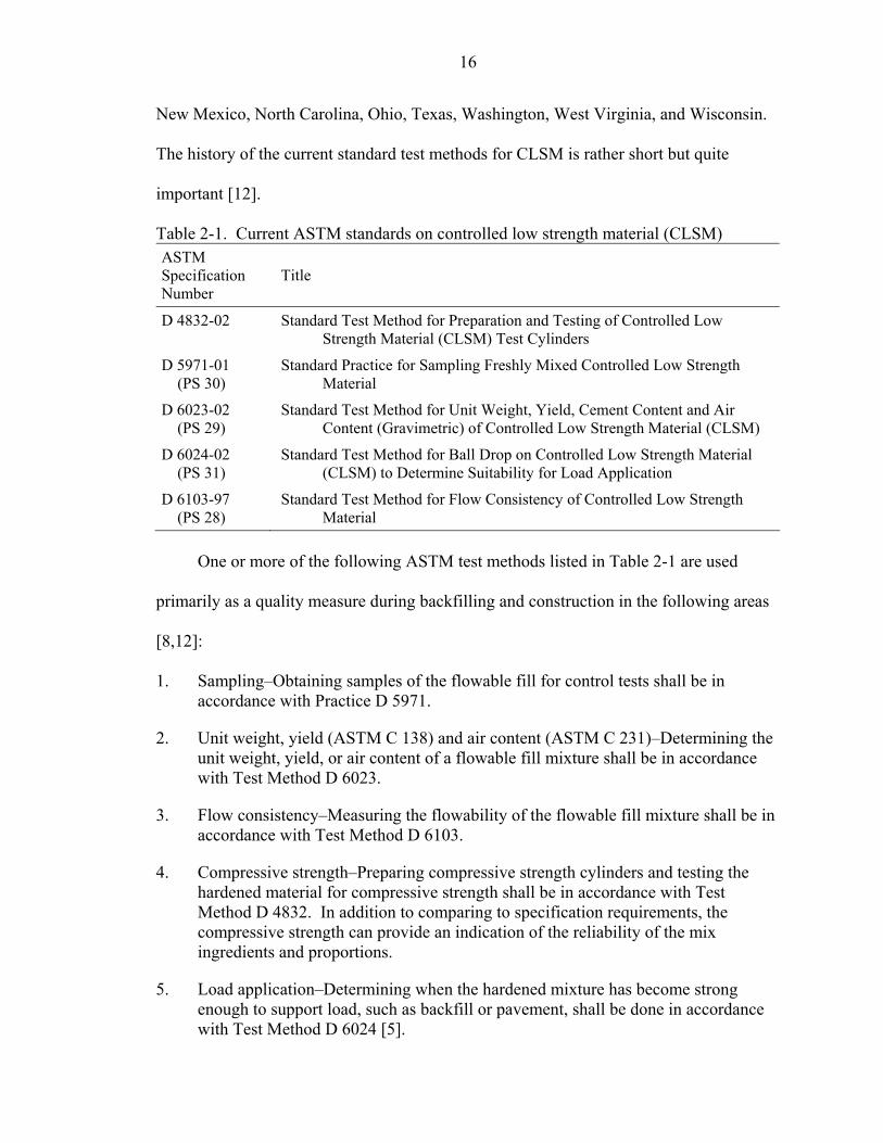
New Mexico, North Carolina, Ohio, Texas, Washington, West Virginia, and Wisconsin.
The history of the current standard test methods for CLSM is rather short but quite
important [12].
Table 2-1. Current ASTM standards on controlled low strength material (CLSM) ASTM Specification Number
Title
D 4832-02
Standard Test Method for Preparation and Testing of Controlled Low Strength Material (CLSM) Test Cylinders
D 5971-01 (PS 30)
Standard Practice for Sampling Freshly Mixed Controlled Low Strength Material
D 6023-02 (PS 29)
Standard Test Method for Unit Weight, Yield, Cement Content and Air Content (Gravimetric) of Controlled Low Strength Material (CLSM)
D 6024-02 (PS 31)
Standard Test Method for Ball Drop on Controlled Low Strength Material (CLSM) to Determine Suitability for Load Application
D 6103-97 (PS 28)
Standard Test Method for Flow Consistency of Controlled Low Strength Material
One or more of the following ASTM test methods listed in Table 2-1 are used
primarily as a quality measure during backfilling and construction in the following areas
[8,12]:
1. Sampling–Obtaining samples of the flowable fill for control tests shall be in accordance with Practice D 5971.
2. Unit weight, yield (ASTM C 138) and air content (ASTM C 231)–Determining the unit weight, yield, or air content of a flowable fill mixture shall be in accordance with Test Method D 6023.
3. Flow consistency–Measuring the flowability of the flowable fill mixture shall be in accordance with Test Method D 6103.
4. Compressive strength–Preparing compressive strength cylinders and testing the hardened material for compressive strength shall be in accordance with Test Method D 4832. In addition to comparing to specification requirements, the compressive strength can provide an indication of the reliability of the mix ingredients and proportions.
5. Load application–Determining when the hardened mixture has become strong enough to support load, such as backfill or pavement, shall be done in accordance with Test Method D 6024 [5].

17
6. Penetration resistance–Tests such as ASTM C 403 may be useful in judging the setting and strength development up to a penetration resistance number of 4000 (roughly 100 psi compressive cylinder strength).
7. Density tests–These are not required since it becomes rigid after hardening.
8. Setting and early strength–These may be important where equipment, traffic, or construction loads must be carried. Setting is judged by scraping off loose accumulations of water and fines on top and seeing how much force is necessary to cause an indentation in the material. ASTM C 403 penetration can be run to estimate bearing strength.
9. Flowability of the CLSM–Flowability is important, so that the mixture will flow into place and consolidate.
Many states have developed specifications governing the use of CLSM. In some
cases, these are provisional. However, specifications differ from state to state, and
moreover, a variety of different test methods are currently being used to define the same
intended properties. This lack of conformity, both on specifications and testing methods,
has also hindered the proliferation of CLSM applications. There are also technical
challenges that have served as obstacles to widespread CLSM use. For instance, it is
often observed in the field that excessive long-term strength gain makes it difficult to
excavate CLSM at later stages. This can be a significant problem that translates to added
cost and labor. Other technical issues deserving attention are the compatibility of CLSM
with different types of utilities and pipes, and the durability of CLSM subjected to
freezing and thawing cycles [13].
2.3.2 ASTM Standard Test Methods
2.3.2.1 Standard Test Method for Preparation and Testing of CLSM Test Cylinders (ASTM D 4832-02)
Cylinders of CLSM are tested to determine the compressive strength of the
material. The cylinders are prepared by pouring a representative sample into molds,
curing them, removing the cylinders from the molds, and capping the cylinders for

18
compression testing. The cylinders are then tested by machine to obtain compressive
strengths by applying a load until the specimen fails. Duplicate cylinders are required
[14].
The compressive strength of a specimen is calculated as follows:
cPfA
= (2-1)
where fc = compressive strength in pounds per square inch (lb/in2); P = maximum failure load attained during testing in pounds (lb); and A = load area of specimen in square inches (in2).
This test is one of a series of quality control tests that can be performed on CLSM
during construction to monitor compliance with specification requirements.
2.3.2.2 Standard Practice for Sampling Freshly Mixed CLSM (ASTM D 5971-96)
This practice explains the procedure for obtaining a representative sample of the
freshly mixed flowable fill as delivered to the project site for control and properties tests.
Tests for composite sample size shall be large enough to perform so as to ensure that a
representative sample of the batch is taken. This includes sampling from revolving-drum
truck mixers and from agitating equipment used to transport central-mixed CLSM [14].
2.3.2.3 Standard Test Method for Unit Weight, Yield, Cement Content and Air Content (Gravimetric) of CLSM (ASTM D 6023-96)
This practice explains the procedure for obtaining a representative sample of the
freshly mixed flowable fill (as delivered). The density of the CLSM is determined by
filling a measure with CLSM, determining the mass, calculating the volume of the
measure, then dividing the mass by the volume. The yield, cement content, and air
content of the CLSM are calculated based on the masses and volumes of the batch
components [14].

19
a) Yield:
1WYW
= (2-2)
where Y = volume of CLSM produced per batch in cubic feet (ft3); W = density of CLSM in pounds per cubic foot (lb/ft3); and W1 = total mass of all materials batched, lb.
b) Cement content:
tNNY
= (2-3)
where N = actual cement content in pounds per cubic yard (lb/yd3); Nt = mass of cement in the batch, lb; and Y = volume of CLSM produced per batch in cubic yards (yd3).
c) Air content:
100T WAT−
= ∗ (2-4)
where A = air content (percent of voids) in the CLSM; T = theoretical density of the CLSM computed on an air free basis, lb/ft3;
and W = density of CLSM, lb/ft3.
2.3.2.4 Standard Test Method for Ball Drop on CLSM to Determine Suitability for
Load Application (ASTM D 6024-96)
This test method is used primarily as a field test to determine the readiness of the
CLSM to accept loads prior to adding a temporary or permanent wearing surface. A stan-
dard cylindrical weight is dropped five times from a specific height onto the surface of
in-place CLSM. The diameter of the resulting indentation is measured and compared to
established criteria. The indentation is inspected for any free water brought to the surface
from the impact [14].
20
2.3.2.5 Standard Test Method for Flow Consistency of CLSM (ASTM D 6103-96)
This test method determines the fluidity and consistency of fresh CLSM mixtures
for use as backfill or structural fill. It applies to flowable CLSM with a maximum
particle size of 19.0 mm (3/4 in.) or less, or to the portion of CLSM that passes a
19.0-mm sieve. An open-ended cylinder is placed on a flat, level surface and filled with
fresh CLSM. The cylinder is raised quickly so the CLSM will flow into a patty. The
average diameter of the patty is determined and compared to established criteria [14].
2.3.3 Other Currently Used and Proposed Test Methods
The American Concrete Institute (ACI) classifies CLSM as a mixture design
having a maximum 28-day compressive strength of 1200 lb/in2. A CLSM mixture that is
considered to be excavatable at a later age using hand tools should have a compressive
strength lower than 101.5 psi at the 28-day stage [14]. This is used to minimize the cost
of excavating a mix at a later stage. Two field requirements that should be specified to
ensure quality control and ease of placement are a minimum level of flowability or
consistency and a specified method of measuring it. Measuring flowability utilizing the
flow cone method is most applicable for grout mixtures that use no aggregate filler. A
maximum flow cone measurement of 35 seconds or a minimum slump of 9 in. would be
two practical design parameters. Other methods to specify CLSM consistency have also
been suggested. One such method is very similar to the ASTM standard test
specification, “Flow Table for Use in Tests of Hydraulic Cement” (C 230), for deter-
mining the consistency or flow of mortar mixtures [14].
Permeability of the CLSM mixtures has been measured using the ASTM “Test
Method for Measurement of Hydraulic Conductivity of Saturated Porous Materials Using
a Flexible Wall Permeameter” (D 5084). Loss on ignition of CLSM mixtures, and

21
mineralogy of the hardened CLSM has been determined on the basis of similar tests for
cement. It has been determined that aggregate containing up to 21% finer than 0.075 mm
could be used to produce a flowable fill mix meeting National Ready Mixed Concrete
Association (NRMCA) performance recommendations [14].
The gradation has been determined per ASTM C136-01, “Standard Test Method
for Sieve Analysis of Fine and Coarse Aggregates” and ASTM C117, “Standard Test
Method for Materials Finer than 75 μm (No. 200) Sieve in Mineral Aggregates by
Washing.” Also, AASHTO M43 #10 screening aggregate specifications [15] has been
used to determine the suitability of utilizing the compliance of aggregates used with these
standards [14].
A new ASTM standard, “Standard Practice for Installing Buried Pipe Using
Flowable Fill” has been proposed, which describes how to use flowable fill for installing
buried pipe. ASTM Committee C 3 on Clay Pipe has already initiated mentioning the use
of flowable fill in the Standard C 12 that covers installation of clay pipe [14].
A summarized overview of the test standards currently in use and that of provi-
sional test methods is as follows [14]:
• Provisional methods of testing
1) AASHTO Designation: X7 (2001)–“Evaluating the Corrosion Performance of Samples Embedded in Controlled Low Strength Material (CLSM) via Mass Loss Testing”
2) AASHTO Designation: X8 (2001)–“Determining the Potential for
Segregation in Controlled Low Strength Material (CLSM) Mixtures” 3) AASHTO Designation: X9 (2001)–“Evaluating the Subsidence of Controlled
Low Strength Materials (CLSM).”

22
• Other ASTM test methods used in CLSM technology
1) ASTM C231-97–“Standard Test Method for Air Content of Freshly Mixed Concrete by the Pressure Method”
2) ASTM C403/C 403M-99–“Standard Test Method for Time of Setting of
Concrete Mixtures by Penetration Resistance” 3) ASTM D560-96–“Standard Test Methods for Freezing and Thawing
Compacted Soil-Cement Mixtures” 4) ASTM D5084-90 (Reapproved 1997)–“Standard Test Method for Measure-
ment of Hydraulic Conductivity of Saturated Porous Materials Using a Flexible Wall Permeameter”
5) ASTM G51-95 (Reapproved 2000)–“Standard Test Method for Measuring
pH of Soil for Use in Corrosion Testing.” 2.3.4 Specifications by the State Departments of Transportation
From a survey of six southeastern states (shown in Table 2-2) carried out by Riggs
and Keck [12], it is apparent that all of the specifications were issued after 1990, and so
the use of CLSM is relatively new to standard transportation road construction. Tables
2-3 and 2-4 show the comparison of similarities and differences for various requirements
based on the survey.
Table 2-2. States surveyed and their specification on flowable fill State Specification and Title of Section Issue Date
Alabama Section 260, Low Strength Cement Mortar 1996 Florida Section 121, Flowable Fill” (revised 1996) 1997 Georgia Section 600, Controlled Low Strength Flowable Fill 1995 North Carolina Controlled Low Strength Material Specification 1996 South Carolina Specification 11, Specification for Flowable Fill 1992 Virginia Special Provisions for Flowable Backfill 1991
According to the survey, the general acceptance age is 28 days with two states
having 56-day requirements (Table 2-3). As a result of the high levels of pozzolans in
many CLSM mixtures, there can be significant strength increases after 28 days. Several
23
states have both excavatable and nonexcavatable mixtures. If the CLSM is to be
removed at a later date, its strength must be limited to less than 300 psi, which can be
assured only if later age strengths are evaluated [12].
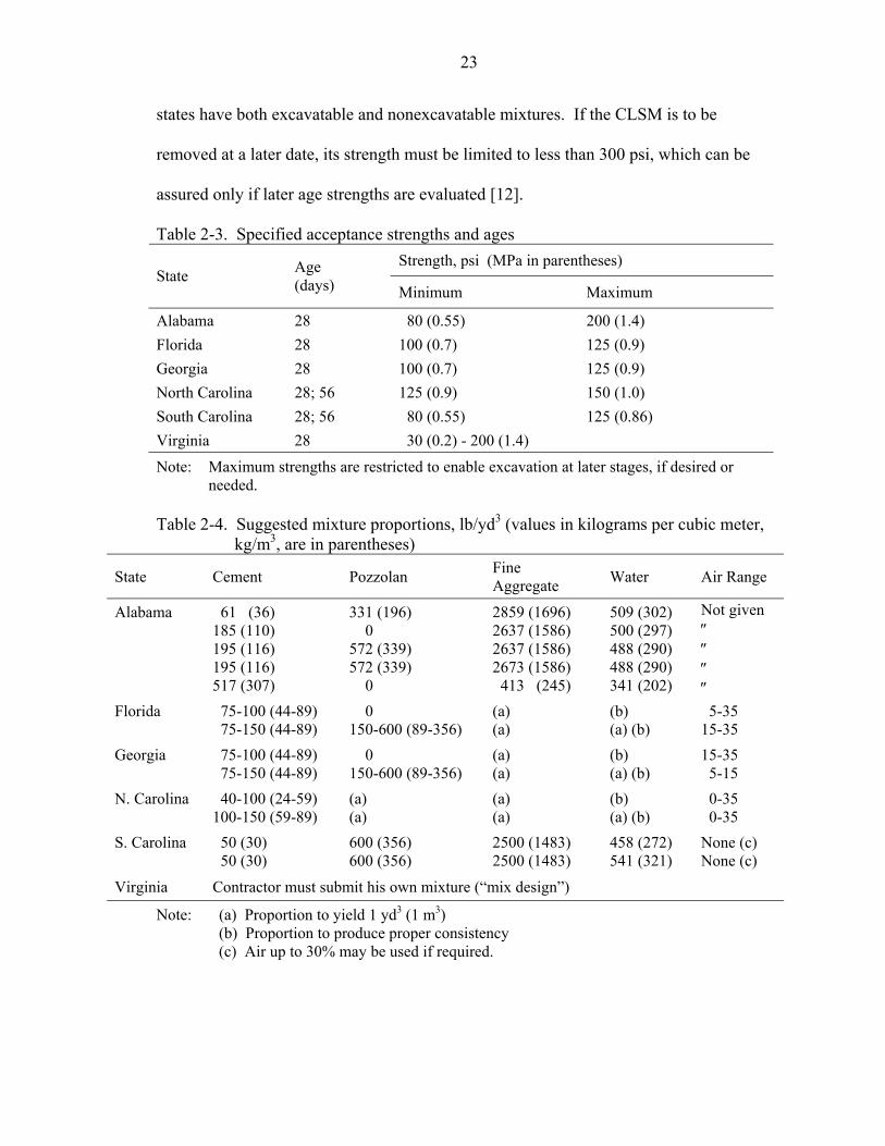
Table 2-3. Specified acceptance strengths and ages Strength, psi (MPa in parentheses)
State Age (days) Minimum Maximum
Alabama 28 80 (0.55) 200 (1.4) Florida 28 100 (0.7) 125 (0.9) Georgia 28 100 (0.7) 125 (0.9) North Carolina 28; 56 125 (0.9) 150 (1.0) South Carolina 28; 56 80 (0.55) 125 (0.86) Virginia 28 30 (0.2) - 200 (1.4)
Note: Maximum strengths are restricted to enable excavation at later stages, if desired or needed.
Table 2-4. Suggested mixture proportions, lb/yd3 (values in kilograms per cubic meter,
kg/m3, are in parentheses)
State Cement Pozzolan Fine Aggregate Water Air Range
Alabama
61 (36) 185 (110) 195 (116) 195 (116) 517 (307)
331 (196) 0 572 (339) 572 (339) 0
2859 (1696) 2637 (1586) 2637 (1586) 2673 (1586) 413 (245)
509 (302) 500 (297) 488 (290) 488 (290) 341 (202)
Not given ″ ″ ″ ″
Florida
75-100 (44-89) 75-150 (44-89)
0 150-600 (89-356)
(a) (a)
(b) (a) (b)
5-35 15-35
Georgia
75-100 (44-89) 75-150 (44-89)
0 150-600 (89-356)
(a) (a)
(b) (a) (b)
15-35 5-15
N. Carolina
40-100 (24-59) 100-150 (59-89)
(a) (a)
(a) (a)
(b) (a) (b)
0-35 0-35
S. Carolina
50 (30) 50 (30)
600 (356) 600 (356)
2500 (1483) 2500 (1483)
458 (272) 541 (321)
None (c) None (c)
Virginia Contractor must submit his own mixture (“mix design”)
Note: (a) Proportion to yield 1 yd3 (1 m3) (b) Proportion to produce proper consistency (c) Air up to 30% may be used if required.

24
2.3.5 Use of Flowable Fill in the State of Florida
Flowable fill has been used throughout the state of Florida as a construction
material. The FDOT has used the material for bedding, encasements, tank enclosures,
pipes, and general backfill for trenches. Occasionally, the use of flowable fill has been
specified for placement under a base with a set time of four hours or more prior to the
placement of the base materials [16].
The current specification divides the flowable fill into two classes: excavatable and
nonexcavatable. The maximum allowable 28-day compressive strength of excavatable
flowable fill is 100 psi. The minimum compressive strength for nonexcavatable flowable
fill is 125 psi. The suggested range of cement and fly ash has been specified for each
class of excavatable and nonexcavatable fill. Prior to use on projects, flowable fill mix
designs must be approved by FDOT. The approval of the mix design is based on the
specified range of material and laboratory test data, such as air content, compressive
strength, and unit weight [16].
2.3.5.1 Material Specifications (Section 121-2)
According to Section 121 of the FDOT “Standard Specifications for Roadway and
Bridge Construction,” the material requirements a flowable fill mix design must meet in
order to be approved by FDOT are noted in Table 2-5 below [16].
Table 2-5. FDOT materials specification requirements Fine aggregatea ...............................................................................Section 902 Portland cement (Types I, II, or III)................................................Section 921 Fly ash, slag and other pozzolanic materials ................................. Section 929 Air-entraining admixturesb .............................................................Section 924 Water...............................................................................................Section 923 aAny clean fine aggregate with 100% passing a 3/8-in. (9.5-mm) mesh sieve and not more than 15% passing a No. 200 (75 µm) sieve may be used.
bHigh air generators or foaming agents may be used in lieu of conventional air-entraining admixtures and may be added at jobsite and mixed in accordance with manufacturer’s recommendation.

25
All materials used should meet other specification requirements on a consistent
basis (see Section 2.3.5.3 below).
2.3.5.2 Construction Requirements and Acceptance (Section 121-5, 121-6)
FDOT specifications require the ambient air temperature to be 40° F (4° C) or
higher and the mix be delivered at a temperature of 50° F (10° C) or higher. FDOT does
not permit placement during rain or when the temperature is below 40° F. Specification
requires the material to remain undisturbed until it reaches a penetration resistance of 35
psi or higher. A soil penetrometer (ASTM C 403, “Standard Test Method for Time of
Setting of Concrete Mixtures by Penetration Resistance”) is used to measure setting time
[16].
2.3.5.3 Guideline for Construction Requirements and Acceptance (Section 121-5, 121-6)
To assist in designing a flowable fill mix, Section 121 of the specifications
provides a guideline shown in Table 2-6 for one to use in preparing a mix design [16].
Table 2-6. FDOT flowable fill mix design Excavatable Nonexcavatable
Cement, Type I
75-100 lb/yd3 (45-60 kg/m3)
75-150 lb/yd3 (45-90 kg/m3)
Fly ash
None
150-600 lb/yd3 (90-335 kg/m3)
Water –a –a Airb 5-35% 5-15% 28-day compressive strengthb
Maximum 100 psi (690 kPa)
Minimum 125 psi (860 kPa)
Unit weightb (wet)
90-110 lb/yd3 (1440-1760 kg/m3)
100-125 lb/yd3 (1600-2000 kg/m3)
aMix design shall produce a consistency that will result in a flowable self-leveling product at a time of placement. bThe requirements for percent air, compressive strength and unit weight are for laboratory designs only and are not intended for jobsite acceptance requirements. Fine aggregate shall be proportioned to yield 1 yd3 (1 m3).

26
2.4 Early Set and Strength Development
2.4.1 Introduction
The early strength of flowable fill in a plastic state comes primarily from the
friction of particles of its constituents. This theory originates from the behavior of
particles in slurry flow, powder technology, and tribology (the science and technology of
interacting surfaces in relative motion and all related practices, including friction,
lubrication, and wear). Although slurry flow does not have any cementing agents, an
explanation of the role of particle friction in slurry is an important base to fully
understanding the early strength of flowable fill.
The end of the plastic state is indicated by hydration of cement particles and the
role of cohesion appears to begin in this stage. The hydration process in flowable fill can
be explained based on the chemical reaction of cement and fly ash in the concrete.
2.4.2 Behavior of Slurries
The behavior of slurries as described by Kendall is similar to that of coulomb
materials, with a flow stress dependent on the high friction between the solid grains [17].
Three simple tests were conducted by Kendall, a plastimeter test, an extrusion test, and a
bubble collapse test. The result was that the slurries became unmoldable, nonextrudable
or noncompactable when the solid grains in the slurry became frictionally locked
together. However, this effect can be prevented by addition of a polymer lubricant which
reduces friction between the grains thereby improving slurry flow.
According to an experiment by Kendall involving wet concrete slurry, if the slurry
is truly plastic, then at a pressure equal to the yield pressure, one’s foot would sink into
the slurry (as in the Bingham model) [17]. In that experiment, the foot did not sink
because the cement grains under the foot were pushed together, experienced friction, and

27
so resisted flow. However, when some polymer lubricant is mixed into the slurry, the
friction between the grains is reduced and the foot does sink through the material. This is
similar to the addition of fly ash particles in flowable fill.
Reynolds, in 1885, conducted an experiment in which a rubber balloon was filled
with sand and water. When the water was excessive, the material was plastic. However
when water was withdrawn from the balloon, the material suddenly became rigid or
dilatant. The rigidity resulted from the higher friction of sand particles since the particles
were pushed closer together, similar to the disappearance of bleeding water in CLSM.
2.4.3 Early Hydration of Cement Particles
In the reaction between cement and water, setting is caused by a selective hydration
of cement compounds. The two compounds first to react are tricalcium aluminate (C3A)
and tricalcium silicate (C3S). However, the addition of gypsum delays the formation of
calcium aluminate hydrate, and instead, ettringite precipitates first from the reaction of
C3A and gypsum, then calcium silicate hydrate (C-S-H) forms from the C3S reaction.
Apart from the rapidity of formation of crystalline products, the development of film
around cement grains and a mutual coagulation of paste components have also been
suggested as factors in the development of setting.
According to Jawed and Skalny, once the nucleation and crystallization of
hydration products end the dormant period, hydration is accelerated by the presence of fly
ash [1]. Fly ash particles provide additional surfaces for the precipitation of the hydration
products, which would otherwise be formed on the surface of the C3S and hinder its
interaction with water. By this account, the jump in early strength development in
flowable fill would occur at the end of the induction period.

28
2.4.4 Influence of Water to the Hydration of Cement
Popovic concluded that the primary factors that influence the times of setting of a
given cement are curing temperature, water/cement (w/c) ratio, and fineness of cement
[2,18]. The times required to set based on the w/c ratio are illustrated in Figure 2-1
below from Soroka [19]. This figure shows that the higher the w/c ratio, the longer the
time required to set up. However, this is only valid for a small range of w/c ratios, which
is 0.25 to 0.85.
0.00
2.00
4.00
6.00
8.00
10.00
12.00
14.00
16.00
0.00 0.20 0.40 0.60 0.80
w/c ratio, by weight
Tim
e of
Set
ting
(hrs
)
Initial SetFinal Set
Figure 2-1. Influence of water/cement (w/c) ratio on the setting of Portland cement paste
[19]
A study by Soroka shows that initially the w/c ratio does not significantly affect the
rate of hydration as indicated by the constant amount of water combined for all mixes
with different w/c ratios [19]. Later, as the w/c ratio lowers, the rate of hydration
decreases, indicated by the smaller amount of water combined in the reactions. Soroka
stated that the lower the w/c ratio, the lower the degree of hydration and the average rate
of hydration. Soroka suggested that this slower rate of hydration may be attributed to the
decrease in the space available for the hydration product at a lower w/c ratio.

29
2.4.5 Effects of Set Accelerator on Hydration of Cement
In the case of calcium chloride accelerator, Rixom and Mailvaganam concluded
that there is no chemical reaction between C3S or dicalcium silicate (C2S) with calcium
chloride, although their rate of reaction is increased [20]. They added that calcium
chloride does not react significantly with cement paste for a period of 2 to 6 hours after
mixing, although rapid setting can occur in this period. Formations of new hydration
products between C3A, gypsum, and calcium chloride may be present. These hydration
products influence the setting behavior of the mix and contribute to higher strength
because more hydration products are formed.
2.4.6 Set Time
In practice, knowledge of the rate of reaction is important because the rate
determines the time of setting and hardening. The initial reaction must be slow enough to
allow time for the flowable fill to be transported and placed. Once it has been placed,
rapid hardening is desirable. In the setting of cement paste, Neville indicates that setting
refers to a change from a fluid to a rigid state and hardening refers to gain of strength
[21]. Although during setting the paste acquires some strength, for practical purposes it
is convenient to distinguish setting from hardening.
Recently, only hardening time has been recognized. Some studies reported that
hardening time refers to the time period required for flowable fill to go from a plastic
state to a hardened state with sufficient strength to sustain loading [21]. These studies
also pointed out that the hardening process is influenced by excess water leaving the
mixture. Excess water leaving the mixture makes the aggregate particles come into
surface contact and the mixture becomes rigid. Also, the cement content has a major
influence on the hardening time.

30
Some research reports that hardening time takes about 3 to 5 hours under normal
conditions. In practice, the extent of hardening is judged by the ability to withstand foot
traffic without surface depression [21].
2.4.7 Strength Development
According to Diamond, the local packing of flocs of cement particles near surfaces
of aggregates or other solids in concrete is poor, and much solution-filled space remains
in the vicinity despite general consolidation of the concrete [22]. Concrete contains little,
if any, bulk uninterrupted cement paste. Diamond pointed out that when water is mixed
with cement, the formation of definite shells of hydration product around cement grains is
the first micro structure development. This occurs after several hours. The shells are
typically of the order of 1 micron in thickness and are usually composed of C-S-H with
some local areas rich in calcium hydroxide (CH) and occasional inward or outward
extensions of ettringite needles or thin calcium monosulfate plates.
A function of fly ash in flowable fill is to provide flowability and fill interparticle
voids if sand is in the mixture. However, when fly ash reacts with cement and water, the
micro structural development is affected. Shells are not only formed around the cement
particles but also around fly ash grains. The shells become tied into a developing skeletal
structure induced by the growth of the cement hydration product. The rate of shell
development around the fly ash particles varies with chemistry and reactivity in the fly
ash. With a fly ash that is low in calcium such as class F fly ash, the shell formation is
followed by a slow reaction on the surface of the fly ash sphere inside the shell.
According to Helmuth in 1987, there has been disagreement concerning the time
the Pozzolanic reaction begins [23]. Some previous workers reported no important
reaction before 28 days but some reported very early reaction. Helmuth said that the
31
reaction appears to begin at an early age, but it does not contribute strength until later.
However, there are conflicting reports about the effect of fly ash in cement hydration.
Some reports indicate an acceleration of C3S hydration, but Jawed and Skalny reported a
pronounced delay of the main heat evolution peak of C3S in the presence of fly ash [1].
The same situation also occurred for C3A.
2.4.8 Use of Mineral Admixture (Fly Ash and Granulated Ground Blast Furnace Slag) in Flowable Fill
A review of the relationship of fly ash and slag as an integral component of the
flowable fill mixture was investigated. Both materials are considered to be mineral
admixtures.
2.4.8.1 Fly ash
Fly ash is a pozzolanic material. Pozzolan is defined as a siliceous or alumino-
siliceous material that possesses little or no cementitious value. Fly ash is a powder
residue that comes from the combustion of pulverized coal in electric power generating
plants. Fly ash is primarily silicate glass containing silica alumina, iron, and calcium.
The minor constituents are magnesium, sulfur, sodium, potassium, and carbon.
According to research by Halverson et al., fly ash is the term generally used to
describe the ash and non-combustible minerals that are released from coal during
combustion and that “fly” up and out of the boiler with the flue gases [24]. The main
constituents in fly ash are oxides, sulfates, phosphates, partially converted dehydrated
silicates, and other inorganic particulate matter residue from coal combustion [25].
Physically, fly ash is made up of fine, powdery particles, which are predominantly
spherical, solid or hollow, and generally in an amorphous state, although uncombusted
carbon in fly ash is usually in the form of angular solid particles [26]. Fly ash has a

32
specific gravity between 2.1 to 3.0 and a specific surface area ranging from 170 to 1000
m2/kg, as determined by the Blaine air permeability test. The Blaine air permeability test,
in accordance to ASTM C 204, measures fineness of a material based on its permeability
to air under specified conditions.
Chemical properties of fly ash are much less consistent than physical properties, as
fly ash is an inherently variable material. Fly ash variability is due to widespread
differences in inorganic chemical constituents of the source coal, methods of coal
preparation, combustion conditions, furnace type, and the ash collection, handling, and
storage conditions at each utility site [27]. Since utilities may not have all these factors in
common, fly ash from different facilities is likely to vary significantly. Even within one
power plant, however, fly ash characteristics can change greatly over time based on load
and operating conditions over a 24-hour period [28]. Consequently, lack of fly ash
consistency is a serious disadvantage in utilizing ash for extensive and economic
beneficial uses.
Despite the uncertainty and variability of fly ash properties, some ash character-
istics can be correlated to the physical and chemical characteristics of the fuel source,
particularly coal. For example, bituminous coal fly ash is predominantly composed of
silica, alumina, iron oxide, and calcium, as well as a variable amount of unburned carbon.
On the other hand, sub-bituminous and lignite coal fly ashes exhibit higher concentra-
tions of calcium and magnesium oxide and lower amounts of silica and iron oxide. These
coals also usually produce fly ash with lower carbon content than that of anthracite [26].
Fly ash color generally varies from tan to gray and black, as a direct function of the
carbon content remaining in the ash [29]. Ash from lignite or sub-bituminous coal is

33
generally tan to beige in color, indicating a low carbon content and the presence of lime
or calcium. Bituminous coal fly ash contains higher unburned carbon and is therefore a
shade of gray. Lighter tints of gray can indicate higher quality ash [26]. Indicated by the
fly ash color, the quantity of unburned carbon carried over from combustion into the fly
ash is measured by the loss on ignition (LOI). High LOI values are undesirable, as they
indicate that the combustion of the source coal is incomplete and raw material is being
carried through to a waste stream rather than being utilized for energy production. LOI is
also a significant chemical property of fly ash and serves as a primary indicator to
whether the ash will make a suitable replacement for cement in concrete production. Fly
ash used as a cement replacement is required by ASTM C618 to have below 6% carbon
content, however, it is preferred to have at or below 3% carbon by members of the
cement and concrete industry [30].
ASTM C618 groups pozzolanic material into three classes: N, F, and C. Class N
refers to natural pozzolans, classes F and C differentiate fly ash of different chemical and
physical properties. Class F is composed of ash produced from burning lignite or
bituminous coal [31]. This class exhibits pozzolanic reactivity but seldom shows any
self-cementitious behavior. Class F fly ash is also termed “low calcium ash,” as it
contains less than 6% calcium oxide (CaO) weight. On the other hand, Class C fly ash is
generated from burning lignite or sub-bituminous coal and typically has higher
concentrations of CaO, generally above 15% by weight [28]. Class C fly ash also
exhibits both pozzolanic and self-cementitious behavior. The function of fly ash in
flowable fill is to provide flowability and to fill interparticle voids for sands in the
mixture.

34
2.4.8.2 Slag
The full correct name for slag is ground granulated blast-furnace slag. In mixtures
of flowable fill and concrete, slag is considered as a cementitious material that can set
and harden in the presence of water. Slag is the heavy, coarse, granular, incombustible
particles remaining in the bottom of coal-fired boilers [32]. Slag is ash, a residue from
combustion in a dry-bottom furnace, consisting of fused ash particles with a size
distribution typically between 75 µm and 2 mm and a composition that depends heavily
on the coal source [28]. Essentially, this product is a waste product from the blast
furnace process for manufacturing of steel and iron. Granulated blast-furnace slag
particles have very porous surface textures that create potential for deterioration during
collection, storage, handling, and use [26]. It is primarily made up of silica, alumina, and
iron, as well as low amounts of calcium, magnesium sulfates, and other inorganic
materials [26]. The chemical characteristics are derived from its coal source and not
operating parameters. Based on its chemical composition and wide range of sizes, slag is
not pozzolanic like fly ash, and therefore, has more limited applications in the cement and
concrete industry [28]. Additionally, its corrosivity, conferred by high salt content and
potentially low pH, limits its use in embankments, road base, subbase, or backfill, where
potential contact with metal structures exists [26].
Slag is often used in the construction industry as a replacement for ordinary
Portland cement. Since slag is a by-product of the iron production process and contains
calcium silicates and aluminosilicates, its cementitious material has been touted for both
its strength and durability-enhancing characteristics when used in concrete. Ground
granulated blast furnace slag also has a lower heat of hydration and, hence, generates less
heat during concrete production and curing. As a result, slag is a desirable material to

35
utilize in concrete placements where control of temperature is an issue. Percentage
replacements by weight of slag for cement have ranged from 10 to 90%.
During the early hydration of the slag, the cement releases alkali metal ions and
calcium hydroxides. The glassy slag structure is broken down and dissolved by the
hydroxyl ions. Initially, the reaction of the slag is with alkali hydroxide; later, the
reaction is primarily with calcium hydroxide [33]. As hydration continues long-term, the
cement continues to precipitate calcium hydroxide and grow rings of C-S-H inward from
the original grain surface. Slag, on the other hand, develops more C-S-H, contributing to
strength, density, and chemical resistance [34].
ASTM C 989 divides ground granulated blast-furnace slag into three strength
grades in accordance with their Slag Activity Index (SAI) values: Grade 80, 100, and
120, with Grade 120 being the most active. The SAI is the ratio of the strength of a 50/50
blend of slag and cement to the strength of a plain cement mix at 7 and 28 days. The SAI
is the criterion used for assessing the relative cementitious potential of slag [33]. How-
ever, the cement used as a reference material must meet minimum requirements of
compressive strength and alkali content. The cement used in a particular project may be
less reactive. In general, the early strengths of Grade 120 slag mixes are lower than other
cement mixtures, but usually catch up and then surpass at 7 days and beyond. It is
commonly believed that the other two grades typically exhibit lower strengths. Factors
which affect slag mix performance and strength development are as follows: 1) propor-
tions of cementitious materials, 2) physical and chemical characteristics of the slag,
3) curing conditions, 4) presence and dosage rate of admixtures, 5) characteristics of the
aggregate, and 6) characteristics of the cement.
36
2.4.8.3 Difference between fly ash and slag
Unlike fly ash which is a pozzolanic, granulated blast-furnace slag is self
cementing. However, when it hydrates by itself, the amount of cementitious products
formed and the rate of formation are insufficient to give adequate strengths for structural
applications. When slag is used in combination with Portland cement, the hydration of
the slag is accelerated in the presence of calcium hydroxide and gypsum. The calcium
hydroxide is also consumed by the slag in a pozzolanic reaction. Proportionally, slag
chemical properties are contain more sulfur trioxide and sulfide sulfur. Thus physically,
slag and fly ash improve the strength gain in flowable fill.
2.4.8.4 Specific applications
Specific applications for both slag and fly ash vary. Both are used extensively in
concrete and flowable fill mixtures. Both materials help to improve the qualities of
flowable fill. One of those qualities involves the workability of flowable fill. For
specific applications involving void filling and backfilling of utility pipes, workability
plays a vital role in flowability of mix and for the complete filling of utility trenches.
2.4.8.5 Mixture proportioning/mixture compliance
According to the review of literature, there is no standard mixture proportioning
adopted by the concrete industry involving mineral admixtures for flowable fill. Many
studies indicate the proportioning of flowable fill is normally specified based on past
experience and the availability of local materials.
A key indicator on a construction jobsite for compliance in a mixture is accom-
plished through visual inspection of the mixture. Excavatable and non-excavatable
flowable fill are distinguishable through mix texture. For example, non-excavatable

37
mixes contain high amounts of cement and fly ash/slag. On the other hand, excavatable
mixes typically contain low amounts of cement and fly ash.
2.4.9 Effect of Moisture on Strength
In concrete, most of the specifications require that it be maintained and tested in a
saturated state. It has been found that dry concrete has higher strength. Mindess and
Young have indicated that the reasons are not completely understood [35]. It is possibly
due to the change in structure of the C-S-H upon drying. Also, a change in internal
friction and cohesion may cause a lubricating effect due to moisture allowing particles to
more easily slip by each other in shear. In addition, the lower compressive strength of
wet concrete may also occur because of the development of internal pore pressures as a
load is applied.
According to Mindess and Young, the ease and extent of slip depends on the forces
of attraction between particles [35]. If the particles are chemically bonded, no slip can
occur, but if only Van der Waals interactions are operating, slip is theoretically possible.
It appears that measurable slip occurs only when sufficient thickness of water exists
between the particles. The water can reduce the Van der Waals forces sufficiently to
allow slippage more readily; it can be thought of as an analogy to lubrication.
Soroka analyzed the decrease of compressive strength of cement paste based on
Griffith’s theory [19]. According to that theory, strength is expected to decrease with an
increase in the moisture content of a material because the presence of absorbed water
reduces specific surface energy. Soroka added that another explanation of the decrease in
strength is the decrease in cohesive forces which results from the presence of absorbed
water. A decrease in the cohesive forces involves weaker bonds between particles.

38
2.5 Strength Prediction Models
2.5.1 Introduction
Past research done on flowable fill has focused on finding ways to better predict the
long-term strength of flowable fill. This section reviews literature published regarding
methods or models developed to predict the strength of flowable fill.
2.5.2 Hamilton County–Removability Index
Specifications developed by Hamilton County, Ohio, and the City of Cincinnati’s,
“Performance Specification for Trench Backfilling Consisting of the Use of Flowable
Fill,” uses the removability index for predicting long-term strength of flowable fill [36].
The removability index, used by Hamilton County, takes into consideration the dry
unit weight (w) in conjunction with the 30-day compressive strength (C′ ). Both are used
to determine removability (excavatability) of a material. A flowable fill mixture is
considered removable if the removability modulus (RE), calculated by the following
equation, is equal to 1.0 or less.
1.5 4 0.5
610 1.010
w CRE′⋅ ⋅
= ≤ (2-5)
where w = dry unit weight (hardened material) (lb/ft3); and C′ = 30-day unconfined compressive strength (lb/in2).
Table 2-7 below shows the removability modulus (RE) values for various combi-
nations of compressive strengths (C′ ) and unit weights (w) calculated by the above
equation. This method of predicting long-term strength is dependent on two variables,
namely, unit weight and the 30-day compressive strength.

39
Table 2-7. Removability modulus (RE) Compressive Strength (C′ ) (psi) w
(lb/ft3) 25 50 75 100 125 150 175 200
50 0.18 0.26 0.32 0.37 0.41 0.45 0.49 0.52
70 0.30 0.43 0.53 0.61 0.68 0.75 0.81 0.86 90 0.44 0.63 0.77 0.89 0.99 1.09 1.17 1.26 110 0.60 0.85 1.04 1.20 1.34 1.47 1.59 1.70 130 0.77 1.09 1.33 1.54 1.72 1.89 2.04 2.18 150 0.96 1.35 1.65 1.91 2.14 2.34 2.53 2.70
Note: RE = 1.15 lb/in2 for hard clay RE = 1.00 lb/in2 for very stiff clay RE = 10.26 for 3000 lb/in2 Portland cement concrete Values in shaded area would not meet the material removability requirement 2.5.3 Bhat’s Study
Some studies utilize parameters involved in mix design for predicting compressive
strength for excavatability. A study by Bhat relates the compressive strength of flowable
fill with the mix w/c ratio [37]. Bhat’s equation shown below uses a single parameter for
predicting strength at 28 days.
3126,905374cS
wc
= +⎛ ⎞⎜ ⎟⎝ ⎠
(2-6)
where Sc = 28-day unconfined compressive strength (KPa); and w/c = water/cement ratio.
According to Bhat, this model is able to correlate strength to w/c ratio (see Figure
2-2). Using Bhat’s equation, the water cement ratios corresponding to a 28-day
compressive strength of 1035 KPa (150 psi) and 690 KPa (100 psi) are approximately 5.8
and 7.4, respectively. The resulting coefficient of determination (R-squared value, R2) is
approximately 80%. This formula used only nonair-entrained flowable fill mixtures
when it was developed.

40
0
100
200
300
400
500
600
0 5 10 15
w/c ratio
28-d
ay U
ncon
fined
C
ompr
essi
ve S
tren
gth,
psi
Figure 2-2. Bhat’s strength prediction model
2.5.4 NCHRP–Study
A study sponsored by the National Cooperative Highway Research Program
(NCHRP), developed two models that predict compressive strength for flowable fill [38].
Equation 2-7, shown below, was developed for predicting strength for air-entrained
mixtures. Equation 2-8 was developed for predicting strength for nonair-entrained
mixtures.
• Prediction equation for air-entrained mixtures ( / )b w c
cf a e′ = ⋅ (2-7)
0.31 ln( ) 0.23a t= ⋅ + 0.01 ln( ) 0.27b t= ⋅ −
where cf ′ = compressive strength (Mpa); and t = age (days).

41
Equation 2-7 was developed using high air content mixtures. It uses w/c ratio as
the predictive factor. Using this formula, one can predict the long-term strength gain
(i.e., beyond a 91-day curing period).
To improve the accuracy of Bhat’s equation, the NCHRP study developed Equation
2-8. Equation 2-8 incorporates the following variables:
1. water/cement (w/c) ratio 2. aggregate type 3. fly ash type; and 4. fly ash content. • Prediction equation for nonair-entrained mixture
( ) ( ) ( ) ( ) ( ) ( )1 2 43( ) ( ) ( )( )0 /
b t b t b tb tagg type fly ash type fly ash contentS t b t k k w c k= ⋅ ⋅ ⋅ ⋅ (2-8)
where b0(t) = −0.0007 · t2 + 0.13 · t – 0.76 b1(t) = −0.0001 · t2 + 0.013 · t – 0.42 b2(t) = −0.00008 · t2 + 0.015 · t – 0.094 b3(t) = −0.003 · t – 1.03 b4(t) = 0.75 – 0.018 · t when t ≤ 30 days b4(t) = 0.22 when t > 30 days S(t) = compressive strength (Mpa); and t = age (days).
The critical aspect to the approach of the NCHRP model was to assign values to the
nonnumerical variables used in the formula. Through a trial-and-error process, the
following constants (k) were recommended for the materials used in the study’s
investigation.
sandriverk = 1.0
sandfoundryk = 0.2
ashbottomk = 1.0
ashCk = 2.2
ashFk = 1.0
ashHCk = 0.75

42
Constants are assigned to aggregate type, fly ash type, and fly ash content
variables. The empirical formula developed by the NCHRP study is an equation that is
readily available for one to use as a guide for designing flowable fill mixes. The formula
employs the variables that are of significance for predicting strength.
2.6 FDOT/UF Flowable Fill Study
A study titled “Use of Accelerated Flowable Fill in Pavement Section” was
conducted for the FDOT at the University of Florida (UF) investigating the usage of
flowable fills in the pavement section [39]. The objective of that study was to evaluate
performance of flowable fill in pavement sections using accelerated and nonaccelerated
mixtures. This evaluation included determination of strength, set time, and flow
applicable to conditions in Florida. The objective was accomplished by replicating
approved FDOT flowable fill mixtures in a laboratory setting. A comprehensive review
of the literature applicable to the research topics was conducted, followed by a survey of
municipalities and counties regarding the use of flowable fill. The unit weight, air
content, and compressive strength were analyzed to establish the conformity of the
contractor-provided mixes and those produced in the lab to FDOT specifications. A
relationship was revealed between the limerock-bearing ratio (LBR) and penetrometer
readings for different mix designs that will help measure the strength of underlying mix
in the field. Unit weights of the mixes depicted substantial variability amongst different
mix designs as well as amongst different districts within the same mix design. However,
a majority of the readings did not comply with FDOT specifications. Similar conclusions
were drawn for the air content of different mixes. The air content for a majority of the
districts were not within the FDOT specified range for both excavatable, as well as
nonexcavatable design mixes. The strength of the flowable fill mixture performance in

43
the laboratory and the strength obtained from collected samples of flowable fill from the
field were evaluated. For the mixtures that were replicated in the laboratory and field
samples being collected, the test yielded better insight and understanding of the
compressive strength of flowable fill at various curing times. The compressive strength
observed was typically above the FDOT specified range for excavatable mixes. For the
nonexcavatable mixes, the compressive strength complied with FDOT specifications,
however its value was considerably high. The relationship between LBR readings and
penetrometer readings was established through regression models. The models were
checked for adequacy.
The previous flowable fill research was successfully completed; however, further
research is necessary to yield a solution for producing flowable fill mixtures capable of
being reproduced and replicated with state DOT’s specifications. This research will
concentrate on developing models for strength and shrinkage prediction, and will
establish a process, define procedures, and create guidelines for future flowable fill
mixtures.

44
CHAPTER 3 MATERIALS AND LABORATORY EXPERIMENTAL PROGRAM
3.1 Introduction
This chapter describes detailed information pertaining to the materials and experi-
mental design evaluated in this study. The method of preparation of the flowable fill
mixtures, design mix selection, mix proportions, fabrication of the test specimens and
testing procedures used in this study are also presented.
3.2 Experimental Design
The objective of this research was to evaluate flowable fill by varying mixture
components to help predict 28-day strength using prediction models. This involves using
excavatable flowable fill.
3.2.1 Rationale for Selecting Mixture Parameters
To meet the research objectives, mixture parameters with ranges were reviewed and
discussed. Particular interest was placed on evaluating parameters affecting flowable fill
strength. Table 3-1 shows the parameters (factors) selected for designing the laboratory
flowable fill mixtures.
A factorial design was employed to acquire insight into the effects of various
mixture parameters on LBR, compressive strength and shrinkage values of excavatable
flowable fill material. According to Montgomery [40], the purpose of a factorial design
is to study the effects of two or more factors. This is an experimental strategy in which
factors are varied together, instead of one at a time. In general, factorial designs are most
efficient for this type of experiment. By factorial design, we mean that in each complete

45
trial or replication of an experiment, all possible combinations of the levels of the factors
are investigated. For example, if there are a levels of factor A and b levels of factor B,
each replicate contains all ab treatment combinations. The mixture parameters, provided
in Table 3-1, include 4 factors. The factors are cement content, air content, mineral
admixtures, and water to cementitious (w/c) ratio. The laboratory study consists of a
4 × 3 × 2 × 3 factorial design. This design summed up to a total of 144 mixtures
including replicates.
Table 3-1. Mixture parameters Mixture Parameters with Ranges
Cement content (4 levels): 50 lb/yd3 100 lb/yd3 50 lb/yd3 200 lb/yd3
Air content (2 levels): 7.5 % ± 2.5% 17.5 % ± 2.5%
Mineral admixtures (3 levels): No admixtures: 0% (1 level) Fly ash class F: 20% (1 level) Granulated ground blast furnace slag: 50% (1 level)
w/c ratio (3 levels): 2.0 4.5 9.0
Slag: 50/50 or 50% slag and 50% Type I cement Fly ash class F: 20/80 or 20% slag and 80% Type I cement
As seen in Table 3-1, the mineral admixtures factor is varied at three levels,
namely, 0%, 20% fly ash, and 50% slag. The 0% indicates a mix with no mineral
admixtures, 20% fly ash indicates a mix containing a 80% cement to 20% fly ash ratio,
and 50% slag indicates a 50% cement to 50% slag ratio.
Appendix A provides the full factorial design matrix along with tables showing the
design of flowable fill batch mix combinations for the experiments. The tables show the
order of the batches categorized into two experiments, Experiment 1 and Experiment 2.
Experiment 1 indicates the treatment combinations and Experiment 2 represents the
replicates. For each experiment, a total of 72 mixtures was generated.

46
The order in which the flowable fill was batched involves the use of numerical
randomization. According to Oehlert [41], randomization is one of the most important
elements of a well-designed experiment. Typically, the process of randomizing involves
the usage of numbers taken from a table of “random” numbers or generated by a
“random” number generator in computer software. The random numbers obtained for the
study were generated using computer software. The spreadsheet software used was
Microsoft® Excel. Random numbers were generated for both experiments separately.
After the numbers were obtained for each batch, they were then sorted into increasing
order.
3.2.2 Mixture Proportioning
The design procedure used in this research project was based on the Absolute
Volume Method (SSD).
Steps in the mixture design calculations are:
1. Calculate absolute volume of cement in cubic feet per cubic yard (ft3/yd3 ) of flowable fill.
62.4
wv
c
CCs
=+
(3-1)
2. Calculate absolute volume of fly ash in ft3/yd3 of flowable fill.
100
62.4
pw w
wv
f
FF C
FFs
= ×
=×
(3-2)

47
3. Calculate absolute volume of slag in ft3/yd3 of flowable fill.
100
62.4
pw w
wv
s
SS C
SSs
= ×
=×
(3-3)
4. Calculate absolute volume of water in ft3/yd3 of flowable fill.
62.4
wv
WW = (3-4)
5. Calculate absolute volume of air content in ft3/yd3 of flowable fill.
27
100p
vA
A×
= (3-5)
6. Calculate absolute volume of saturated-surface-dry (SSD) for fine aggregate in ft3/yd3 of flowable fill.
( )27vs v v v vFA C F W A= − + + + (3-6)
7. Calculate weight of saturated-surface-dry in pounds per yard (lb/yd) of flowable fill.
62.4ws vs agFA FA S= × × (3-7)
8. Calculate weight of fine aggregate base on natural moisture content in pounds per cubic yard (lb/yd3 ) of flowable fill.
11wn ws
NFA FAL
+= ×
+ (3-8)
9 . Correct the weight of water due to percentage of moisture difference in lb/yd3 of flowable fill.
ws wn
w
W FA FA
W W W
Δ = −
= + Δ (3-9)
where Cv = absolute volume of cement, ft3/yd3 Cw = weight of cement, lb/yd3

48
Sc = specific gravity of cement Fw = weight of fly ash, lb/yd3 Fp = percent of fly ash by weight of cement Fv = absolute volume of fly ash, ft3/yd3 Sf = specific gravity of fly ash Sw = weight of slag, lb/yd3 Sp = percent of slag by weight of cement Sv = absolute volume of slag, ft3/yd3 Ss = specific gravity of slag Wv = absolute volume of actual water, ft3/yd3 Ww = weight of actual water, lb/yd3 Av = absolute volume of air, ft3/yd3 Ap = percent of air content FAvs = absolute volume of saturated-surface-dry fine aggregate, ft3/yd3 FAws = weight of saturated-surface-dry fine aggregate, lb/ft3/yd3 Sag = specific gravity of aggregate FAwn = weight of fine aggregate base on natural moisture content, lb/yd3 N = percent of natural moisture content L = percent of absorption ΔW = weight of water due to percentage of moisture different, lb/yd3;
and W = water requirement, lb/yd3.
Typical computations are presented in Appendix A. Appendix A also provides
tables showing the volume computation results per combination of batch mix. The tables
provide computation results for both 1 yd3 and 5.5 ft3 mix volumes. A sand-to-water
ratio column is provided within the tables. The sand-to-water ratio was found beneficial
throughout the research for helping to determine whether a mixture is feasible or non-
feasible prior to mixing. Mixtures with a sand-to-water ratio range of 1.73 to 7.20 were
deemed feasible and those out of that range were classified as non-feasible.
This type of classification system was defined at the early stages of the research
study through trial mixing and from the early part of batch mixing. It was important to
see whether a mix was feasible or non-feasible for the purpose of time constraint.

49
3.2.3 Specimen Sample Collection per Batch Mix
The size and test samples to be collected from each batch are summarized below.
Table 3-2 summarizes the overall specimen samples required for each batch mix. As
shown, the total number of samples required for collection per mix is 33. The number of
samples needed per mix and the type of specimen samples (i.e., 18 LBR and 15 plastic
cylinder molds) helped determine the design of the experiment. The 33 samples collected
per mix provided the basis for total volume of flowable fill needed for each mix.
Table 3-2. Summary of sample specimens collected per mix
Curing Period No. of Samples (LBR) No. of Samples (4-in. × 8-in. cylinders)
6 hrs 3 -- 24 hrs 3 3 3 days 3 3 28 days 3 3 56 days 3 3 Oven cured, 2 days 3 -- Total 18 15a
Number of samples per mixtures = 33 Volume of each LBR mold = 169.65 in3 = 0.10 ft3 Volume of each 4 × 8 cylinders = 100.53 in3 = 0.0582 ft3 Volume of each 6 × 12 cylinders = 339.29 in3 = 0.1963 ft3 Total volume required to fill samples per batch mix: Volume = (18 × 169.65 + 12 × 100.53 + 3 × 339.29) in3 = 5277.93 in3 = 3.0544 ft3 aTotal includes three 6 × 12 cylinder samples produced for shrinkage testing.
Table 3-2 also shows the curing durations used for all the samples collected per
batch of mix. The volume of mix per batch was based on the total number of samples
needed per mix. As illustrated, an approximate volume of 3.0544 ft3 of flowable fill was
determined to be the required amount per batch of mix.
3.2.4 Specimen Molds
The specimen molds employed for the research can be categorized as cylindrical
LBR molds, either 4-in. × 8-in. or 6-in. × 12-in. test cylinders. The cylindrical LBR
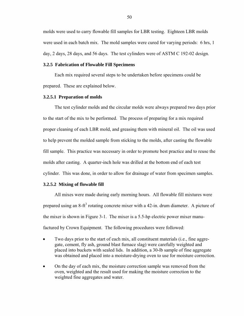
50
molds were used to carry flowable fill samples for LBR testing. Eighteen LBR molds
were used in each batch mix. The mold samples were cured for varying periods: 6 hrs, 1
day, 2 days, 28 days, and 56 days. The test cylinders were of ASTM C 192-02 design.
3.2.5 Fabrication of Flowable Fill Specimens
Each mix required several steps to be undertaken before specimens could be
prepared. These are explained below.
3.2.5.1 Preparation of molds
The test cylinder molds and the circular molds were always prepared two days prior
to the start of the mix to be performed. The process of preparing for a mix required
proper cleaning of each LBR mold, and greasing them with mineral oil. The oil was used
to help prevent the molded sample from sticking to the molds, after casting the flowable
fill sample. This practice was necessary in order to promote best practice and to reuse the
molds after casting. A quarter-inch hole was drilled at the bottom end of each test
cylinder. This was done, in order to allow for drainage of water from specimen samples.
3.2.5.2 Mixing of flowable fill
All mixes were made during early morning hours. All flowable fill mixtures were
prepared using an 8-ft3 rotating concrete mixer with a 42-in. drum diameter. A picture of
the mixer is shown in Figure 3-1. The mixer is a 5.5-hp electric power mixer manu-
factured by Crown Equipment. The following procedures were followed:
• Two days prior to the start of each mix, all constituent materials (i.e., fine aggre-gate, cement, fly ash, ground blast furnace slag) were carefully weighted and placed into buckets with sealed lids. In addition, a 30-lb sample of fine aggregate was obtained and placed into a moisture-drying oven to use for moisture correction.
• On the day of each mix, the moisture correction sample was removed from the oven, weighted and the result used for making the moisture correction to the weighted fine aggregates and water.
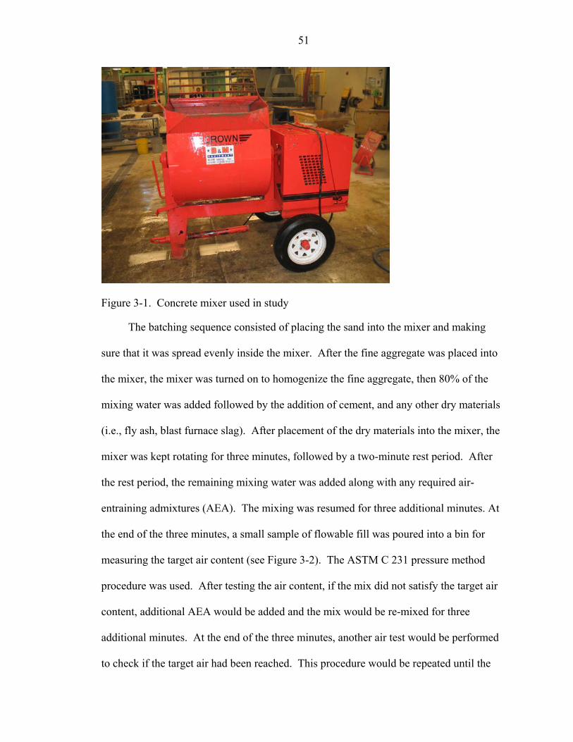
51
Figure 3-1. Concrete mixer used in study
The batching sequence consisted of placing the sand into the mixer and making
sure that it was spread evenly inside the mixer. After the fine aggregate was placed into
the mixer, the mixer was turned on to homogenize the fine aggregate, then 80% of the
mixing water was added followed by the addition of cement, and any other dry materials
(i.e., fly ash, blast furnace slag). After placement of the dry materials into the mixer, the
mixer was kept rotating for three minutes, followed by a two-minute rest period. After
the rest period, the remaining mixing water was added along with any required air-
entraining admixtures (AEA). The mixing was resumed for three additional minutes. At
the end of the three minutes, a small sample of flowable fill was poured into a bin for
measuring the target air content (see Figure 3-2). The ASTM C 231 pressure method
procedure was used. After testing the air content, if the mix did not satisfy the target air
content, additional AEA would be added and the mix would be re-mixed for three
additional minutes. At the end of the three minutes, another air test would be performed
to check if the target air had been reached. This procedure would be repeated until the

52
Figure 3-2. Pressure meter test for air content
target or acceptable level of air content was achieved. It was often found to be challeng-
ing to obtain both the desired air and water contents. For relatively dry flowable fill,
adding AEA would increase the air content. For mixtures that were very fluid or had
high flow, it was found to be very difficult to obtain 1 to 2% air content or air content
near the target. The experience gained from trial mixing allowed more efficient
converging to the target air content for each flowable fill mixture.
Immediately after mixing, flowable fill was poured into a large bin container for
transportation and subsequent transfer into specimen molds. Prior to pouring into
specimen molds, a sample of the fresh mix was taken so that other plastic property
measurements, such as unit weight, temperature, and flow tests could also be performed
on the mix. Each specimen mold was properly marked and labeled for identification and
testing purposes.
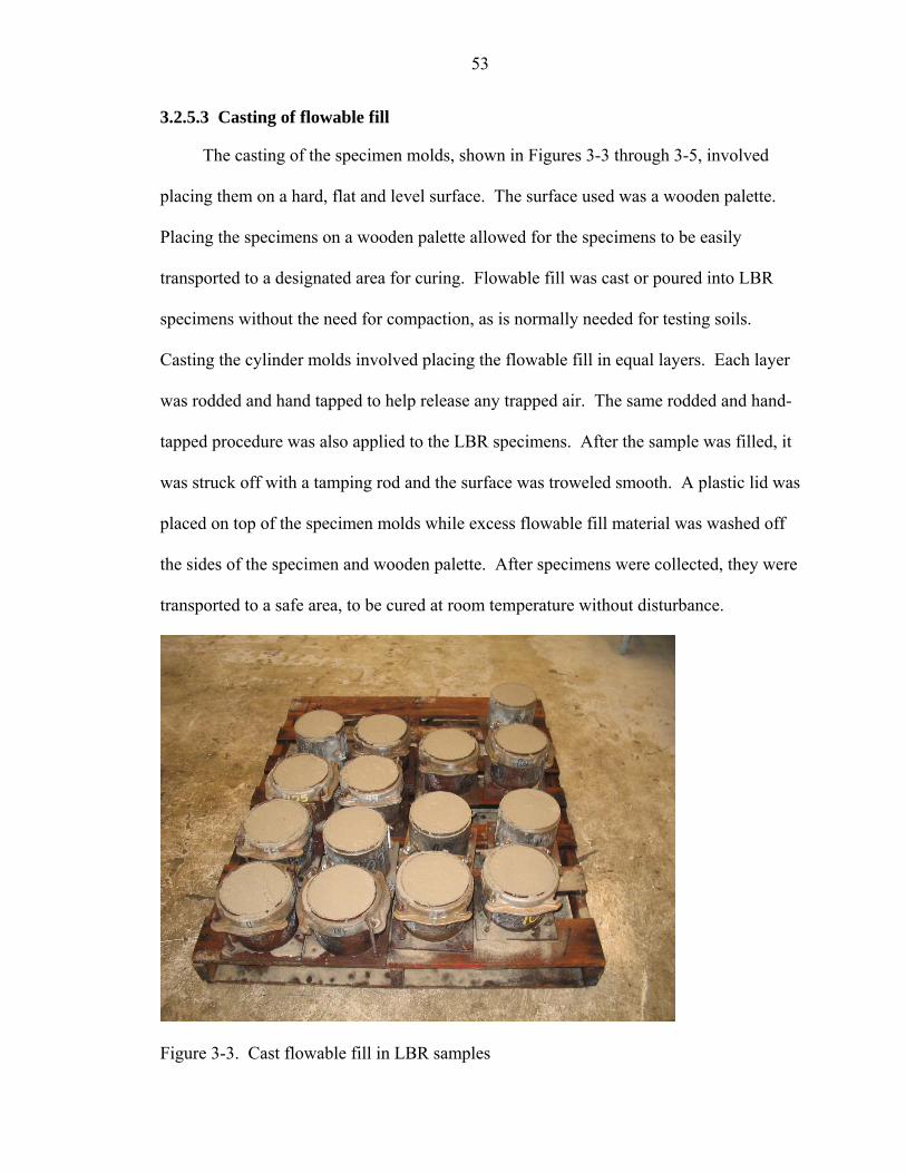
53
3.2.5.3 Casting of flowable fill
The casting of the specimen molds, shown in Figures 3-3 through 3-5, involved
placing them on a hard, flat and level surface. The surface used was a wooden palette.
Placing the specimens on a wooden palette allowed for the specimens to be easily
transported to a designated area for curing. Flowable fill was cast or poured into LBR
specimens without the need for compaction, as is normally needed for testing soils.
Casting the cylinder molds involved placing the flowable fill in equal layers. Each layer
was rodded and hand tapped to help release any trapped air. The same rodded and hand-
tapped procedure was also applied to the LBR specimens. After the sample was filled, it
was struck off with a tamping rod and the surface was troweled smooth. A plastic lid was
placed on top of the specimen molds while excess flowable fill material was washed off
the sides of the specimen and wooden palette. After specimens were collected, they were
transported to a safe area, to be cured at room temperature without disturbance.
Figure 3-3. Cast flowable fill in LBR samples

54
Figure 3-4. Cast flowable fill in 4-in. × 8-in. (compressive strength) samples
Figure 3-5. Cast flowable fill in 6-in. × 12-in. (volume change) samples

55
The tests run on fresh flowable fill followed the ASTM standards shown in Table
2-1. These ASTM test methods are used primarily as a quality measure. Temperature of
the fresh flowable fill was determined in accordance with the ASTM C 1064 standard.
This test was used to ensure that the temperature of the fresh flowable fill was within
normal range and to ensure no unexpected conditions in the mix. A digital thermometer
was used to monitor mix temperature during plastic test.
The measured plastic properties for each flowable fill mixture are summarized in
Tables 3-3 and 3-4, shown below. The results of the mixtures are presented in the order
in which they were batched. As previously specified, the order of the mix is based on
their assigned random number. Note that mixtures marked with a superscript “a”
represent mixtures batched for a third time due to equipment malfunctions during
batching or testing. In Table 3-4 mixture numbers ending in “R” denote mixtures that
were replicated for statistical purposes; mixtures denoted with the term “Type I” are
mixes batched using ASTM Type I Portland cement.
3.3 Limerock Bearing Ratio Test (Florida Test Method 5-515)
The Limerock Bearing Ratio (LBR) test was adopted by the Florida Department of
Transportation (FDOT) as a standard strength test for subgrade and base materials in the
1960’s [42]. The LBR test is a modified version of the California Bearing Ratio (CBR)
test. This test defines the ability of a soil to support a load. As part of this test, the
maximum density of the soil is determined by the standard ASTM D-1557 method. CBR
was renamed LBR because the standard strength for the CBR test was changed to more
closely represent Florida materials. Some minor procedural changes to the LBR test have
also evolved over the years. The LBR test, as used in flexible pavement design in
Florida, is a measure of the bearing capacity of soil. The test consists of measuring the

56
Table 3-3. Properties of fresh flowable fill (Experiment 1)
Air Content (%) Batch Mix Number
AEAa (ml)
Flow (in.) Target Achieved
Unit Weight (lb/t3)
Mixture Temperature (° F)
4 NR 4.25 7.5 ± 2.5 22.00 100.80 68.00 25 NR 0.00 7.5 ± 2.5 5.20 120.32 68.40 15 NR 0.00 7.5 ± 2.5 7.60 121.04 70.00 23 NR 0.00 7.5 ± 2.5 5.50 122.24 69.00 50 100 5.25 17.5 ± 2.5 17.00 107.04 76.00 16 1600 4.25 7.5 ± 2.5 1.30 126.80 71.00 61 200 6.50 17.5 ± 2.5 20.00 103.28 70.00 34 500 4.50 7.5 ± 2.5 1.00 124.76 70.00 24 1000 0.00 7.5 ± 2.5 1.20 127.84 70.00 59 1000 6.00 17.5 ± 2.5 4.80 125.92 72.00 58 100 5.50 17.5 ± 2.5 18.00 111.52 73.00 51 1000 10.50 17.5 ± 2.5 7.80 121.04 76.00 69 200 7.00 17.5 ± 2.5 40.00 111.52 71.00 26 500 4.00 7.5 ± 2.5 1.40 129.20 72.00 40 200 7.00 17.5 ± 2.5 20.00 106.00 70.00 16b 500 7.00 7.5 ± 2.5 0.80 132.08 72.00 14 10 0.00 7.5 ± 2.5 15.00 112.24 72.00 8 250 5.00 7.5 ± 2.5 21.00 103.12 78.00 30 500 0.00 7.5 ± 2.5 2.00 128.08 71.00 18 25 0.00 7.5 ± 2.5 13.00 114.24 70.00 20 500 0.00 7.5 ± 2.5 0.60 129.52 72.00 44 75 5.50 17.5 ± 2.5 15.20 111.60 79.00 65 75 8.00 17.5 ± 2.5 15.00 110.16 76.00 54 25 0.00 17.5 ± 2.5 16.00 109.84 78.00 55 500 7.00 17.5 ± 2.5 7.40 124.24 78.00 12 25 0.00 7.5 ± 2.5 15.00 110.08 78.00 22 25 0.00 7.5 ± 2.5 18.00 106.72 77.00 33 25 0.00 7.5 ± 2.5 18.50 107.84 73.10 19 500 9.00 7.5 ± 2.5 4.50 125.44 73.20 48 175 6.75 17.5 ± 2.5 25.00 106.64 73.00 4b 25 0.00 7.5 ± 2.5 16.00 110.32 71.00 69b 25 4.25 17.5 ± 2.5 17.00 115.44 70.50 Note: aNR = Not recorded bmixtures batched for a third time due to malfunctions during batching or testing

57
Table 3-4. Properties of fresh flowable fill (Experiment 2) Air Content (%) Batch Mix
Numbera AEAb (ml)
Flow (in.) Target Achieved
Unit Weight (lb/t3)
Mixture Temperature (° F)
8R 250 7.50 7.5 ± 2.5 24.50 99.92 70.00 16R 500 0.00 7.5 ± 2.5 0.50 129.36 72.00 30R 500 0.00 7.5 ± 2.5 2.00 129.12 72.00 18R NR 0.00 7.5 ± 2.5 15.50 116.88 71.00 14R NR 0.00 7.5 ± 2.5 13.00 116.88 75.00 22R NR 0.00 7.5 ± 2.5 19.50 109.68 76.00 33R 25 0.00 7.5 ± 2.5 17.50 107.44 76.00 23R 600 7.75 7.5 ± 2.5 7.10 123.44 74.50 15-Type I 300 0.00 7.5 ± 2.5 7.00 123.68 75.00 54-Type I 25 0.00 17.5 ± 2.5 15.00 115.28 76.00 25-Type I 25 0.00 7.5 ± 2.5 20.00 107.52 75.00 48-Type I 50 6.00 17.5 ± 2.5 20.00 108.16 75.00 25R 25 0.00 7.5 ± 2.5 17.00 108.24 75.00 34R 500 5.25 7.5 ± 2.5 2.50 127.76 75.00 69R 50 6.00 17.5 ± 2.5 20.00 105.12 74.00 26R 500 6.25 7.5 ± 2.5 1.00 127.84 75.00 40R 125 6.50 17.5 ± 2.5 24.00 102.40 79.00 19R 500 10.00 7.5 ± 2.5 6.10 124.96 74.50 44R 75 5.00 17.5 ± 2.5 18.00 108.72 78.00 48R 25 0.00 17.5 ± 2.5 15.00 112.24 75.00 55R 500 8.50 17.5 ± 2.5 3.20 128.88 75.00 54R NR 0.00 17.5 ± 2.5 14.50 115.12 75.50 4R 25 0.00 7.5 ± 2.5 15.00 117.04 75.00 58R 75 5.00 17.5 ± 2.5 16.50 110.08 74.50 12R 25 0.00 7.5 ± 2.5 12.00 117.52 75.00 15R 550 7.50 7.5 ± 2.5 5.20 125.36 75.00 20R 500 0.00 7.5 ± 2.5 1.10 127.6 75.00 65R 75 6.00 17.5 ± 2.5 17.00 108.8 75.00 61R 150 8.50 17.5 ± 2.5 21.00 101.76 76.00 59R 1000 9.00 17.5 ± 2.5 6.30 123.52 78.00 51R 1000 7.50 17.5 ± 2.5 8.00 120.24 71.00 24R 1000 6.50 7.5 ± 2.5 1.70 127.76 69.00 50R 100 6.50 17.5 ± 2.5 19.00 105.60 70.00 25Rc 25 0.00 7.5 ± 2.5 17.00 108.72 70.00 48Rc 25 0.00 17.5 ± 2.5 14.50 111.84 80.00 55Rc 500 5.50 17.5 ± 2.5 5.70 123.12 75.00 Note: aR in mixture number = mixtures that were replicated for statistical purposes; Type I in mixture number = mixes batched using ASTM Type I Portland cement bNR = Not recorded cmixtures batched for a third time due to malfunctions during batching or testing

58
load required to cause a standard circular plunger (an area of 3 in2) to penetrate the soil
specimen at a specified rate (refer to Figures 3-6 and 3-7). The specifications for the
LBR test equipment are included in Table 3-5. The LBR test measures the unit load (in
lb/in2) required to force the plunger into the soil 0.1 in., expressed as a percentage of the
unit load in lb/in2, required to force the same plunger to the same depth in a standard
sample of crushed limerock.
10-lb seating load
Magnetic clamp
Penetration piston end area 3 sq. in. (1.95 in. dia. ±.01 in.)
.001 in. indicating dial measuring penetration
Surcharge weights (as required)
Mold 6 in. internal dia.
No. 4, 15-cm filter paper
Soil sample 6 in. dia. × 4.59 in. high
Perforated base
Figure 3-6. Cross section of seated LBR penetration piston [42]

59
Figure 3-7. LBR machine
Table 3-5. Specifications for LBR test equipment Equipment Specifications
LBR Press Rainhart Company, Model 762 Rate of loading: .050 in./minute Load cell capacity: 10,000 lbs
LBR Recording Device GPE, Inc., Model DMP-12A Digital LBR readout Proprietary plot program RS 232 communications port Download to computer: Windows XP
System Calibration Device Steel spring soil simulator at 100 LBR ±5 LBR

60
The average penetration unit load for a typical crushed limerock found in Florida
has been standardized to 800 lb/in2. The resulting ratio multiplied by 100 is known as the
Limerock Bearing Ratio (with percentage omitted). The test results are intended to
provide the relative bearing value of base and stabilized materials [42].
Samples are tested by penetrating the specimens. This is accomplished with an
automatic compression device equipped with a load measuring system. A typical test is
shown and the penetration curve is plotted in Figures 3-8 and 3-9, respectively. The
corrected unit load obtained at 0.1-inch penetration is divided by 800 lb/in2, the standard
strength of limerock. This ratio is then multiplied by 100, and the resulting value is the
LBR in percent, as shown in equation below.
Corrected Unit LoadLBR 100800
= × (3-10)
The load penetration relationship curve will usually be convex upwards although
the initial portion of the curve may be concave upwards. The concavity is assumed to be
due to surface irregularities (Figure 3-9). A correction is applied by drawing a tangent to
the curve at the point of greatest slope. The corrected curve then becomes the tangent
plus the convex portion of the original curve with the origin moved to the point where the
tangent intersects the horizontal axis. Methods of correcting typical curves are illustrated
in Figures 3-8 and 3-9.
3.4 Compressive Strength Test
Although there is an existing standard method for measuring the unconfined
compressive strength of flowable fill (ASTM D 4832), a different method was utilized for
this research. Compressive strength tests were performed according to ASTM method
D-2166-00 (AASHTO T 208-05). This test covers the determination of the unconfined

61
Figure 3-8. Graph example showing typical load penetration curve that requires no
correction [42]

62
Figure 3-9. Graph example showing correction of typical load penetration curve for
small surface irregularities [42]

63
compressive strength of cohesive soil in the undisturbed, remolded, or compacted
condition, using strain-controlled application of the axial load. The test method provides
an approximate value of the strength of cohesive soils in terms of total stresses. The
method of testing was selected due to the low strength of flowable fill and the
resemblance of its properties to cohesive soils. The compression tests were performed
using a computerized testing machine with a relatively low-load capacity machine with
displacement control. For this research the compression machine used was equipped
with a 2000-lb load cell. The apparent strain rate was set at 0.015 inches per minute.
The linear voltage displacement transducer (LVDT) used was a 2-inch MPE type HS.
The load frame was a 5-ton compression machine, manufactured by Wykeham Farrance.
Figure 3-10 shows the set up for the compressive strength test. The compressive strength
of the test specimen is calculated by dividing the maximum load attained from the test by
the cross-sectional area of the specimen.
Figure 3-10. Typical set-up for compressive strength test

64
Before testing the flowable fill specimen, it was removed from its plastic cylinder
mold. Removing the specimen from the mold involved careful handling due to its low
strength (as compared to hardened concrete cylinders). The cylinders were cut length-
wise, using a box cutter. Specimens were kept in molds until the day of testing.
3.5 Proctor Penetrometer Test
Penetration resistance of the LBR mold specimens were obtained using the proctor
penetrometer testing method outlined in ASTM D 1558-99. In this test, a cylindrical
needle tip is pressed one inch into the flowable fill at a constant rate, and the resistance
offered by the flowable fill is measured in pounds. This value (in pounds) is divided by
the cross sectional area of the tip in square inches, and is taken as the penetration
resistance in pounds per square inch (psi). Since different needle tip diameters exist, the
choice of needles selected depended on the strength of the material being tested. Figure
3-11, shown below, depicts the proctor penetrometer device in its carrying case with a
complete set of penetrometer needles. The needles have end areas of 1 in2, 3/4 in2, 1/2
in2, 1/3 in2, 1/5 in2, 1/10 in2, 1/20 in2, 1/30 in2, and 1/40 in2. The psi values obtained
Figure 3-11. Typical proctor penetrometer

65
from the proctor penetrometer are not equivalent to the psi values obtained from
unconfined compressive strength tests.
3.6 Drying Oven
A standard laboratory oven with approximately 6 ft3 of capacity was used for
curing of oven specimen samples. LBR samples were stored inside the oven at a set
temperature of 110° F. The oven is equipped with a thermostat and sensor to control the
temperature of the oven. Prior to the start of every mix, the oven was turned on to ensure
that it would be warm enough to place specimens inside. Information acquired from
specimens cured in the oven would help predict in-service aging.
3.7 Drying Shrinkage of Flowable Fill Mixtures
For each flowable fill mixture batched, three 6-in. × 12-in. cylinders were made to
evaluate its shrinkage behavior due to volume change. The cylinders were cured under
normal conditions.
Currently, no standard test methods exist for the measurement of drying shrinkage
in flowable fill. As a result, a review of published studies was done to identify standard
methods of testing of drying shrinkage in flowable fill. Most of the published studies
reviewed showed the use of the conventional concrete method to measure shrinkage of
flowable fill specimens (7). This method specifies embedding gage studs at both ends of
a specimen and measuring the length change. Careful handling of the shrinkage prisms
during form removal and subsequent measurements is required. Flowable fill specimens
could be damaged when using this approach because of the lower strengths of flowable
fill. Thus, this approach may not be appropriate for flowable fill. Another approach
found for measuring shrinkage in flowable fill was used by Lutcht (43). In his study,

66
Lutcht used the shrinkage ring method to measure shrinkage in flowable fill. Typically, a
shrinkage ring is used to measure the cracking of concrete cast around a steel ring. The
approach utilized by Lutcht is not an adopted standard and thus represents 100% restraint
and is used for assessing different materials and mixtures. Using the knowledge gained
from other research studies, various attempts and methods were devised to measure the
volume change that occurs in flowable fill.
3.7.1 Method 1
The first method used to measure the drying shrinkage in flowable fill was
somewhat similar to the ASTM C157 standards used for measuring drying free shrinkage
in concrete. ASTM C157 standards call for using square prism specimen molds with
dimensions of 3 × 3 × 11.25 inches. All of procedures of the ASTM C157 standards
were followed, with the exception of the specimen molds. Instead of using square prism
molds, 6-in. × 12-in. cylinders were used.
The amount of shrinkage was measured with a linear voltage displacement
transducer (LVDT) of an accuracy of 0.00039 in., which measured displacement. The
LVDTs used for this project were made of AISI 400 series stainless steel. They are
complete and ready-to-use displacement transducers with a sleeve bearing structure on
one end that supports a spring-loaded shaft attached to the core. The bearing is threaded
externally to facilitate mounting. By using a spring loaded LVDT, the need for core rods
or core support structures is eliminated. All LVDTs are hermetically sealed to operate in
harsh environments such as a moist room and have an operating temperature range of
0° F to 160° F (−17.8° C to 71.1° C) to facilitate testing of temperature effects.

67
The data acquisition system used was an Agilent 34970A unit (by Agilent
Technologies) with a HP 34901A (20-channel armature multiplexer) plug-in module.
The data acquisition unit can be set up to take readings at specified time intervals and for
a specified length of time. The HP 34901A multiplexer module can read up to 20
channels of AC or DC voltages with a maximum capacity of 300 V. It has a switching
speed of up to 60 channels per second. It also has a built-in thermocouple reference
junction for use in temperature measurement by means of thermocouples. Thus, the
Agilent 34970A data acquisition unit with one HP 34901A multiplexer module will be
adequate for the job of recording load and displacement readings from ten testing
apparatuses. The Agilent 34970A unit can take up to three plug-in modules. Thus, if
needed, it can be expanded to take up to 60 channels of output.
The test setup for measuring the free shrinkage using LVDT is shown in Figures
3-12 and 3-13. Figure 3-12 is a photograph of several test set-ups that were used,
simultaneously, while Figure 3-13 is the schematic of these test set-ups. Three sets of
measurements were taken from each specimen. A total of nine sets of measurements
were taken from the three replicate specimens for each flowable fill mixture. Shrinkage
measurements were taken at 1-, 3-, and 7-day intervals.
The setup for the ASTM C157 free shrinkage test consisted of a DC-powered
LVDT connected to a shrinkage test frame that held the specimen. The output from the
LVDT was connected to a Data Acquisition System (DAS). A laptop computer was used
to download the data from the DAS. The data downloaded from the Data Acquisition
System was in readable form with Microsoft Excel “Comma Separated Variable” format.

68
Figure 3-12. Test set-up for measuring shrinkage using LVDTs
Figure 3-13. Schematic of test set-up for measuring shrinkage using LVDTs

69
3.7.2 Method 2
The second method for measuring drying shrinkage in the flowable fill specimen
utilized a dial gauge. The process involved filling the cylinder mold with flowable fill,
finishing the surface, and then leveling it off with the cylinder top. This provided a 12-in.
gauge length and 0.000-in. initial reading. When the readings were taken, the plunger of
the dial gauge was placed in the center of the cylinder and then lowered until the bridge
set on top of the cylinder mold. A total of three readings were taken at 1-, 4-, and 7-day
intervals.
Figures 3-14 and 3-15 provide images of flowable fill specimen cylinders with the
gauge being used. For this method, the gauge is used to measure the change in the
specimen height which occurs as the flowable fill specimen volume changes or shrinks
(final height, hf, of flowable fill specimen). The dial gauge used has an accuracy reading
Figure 3-14. Three-dial gauge reading method (gauge placed on level flowable fill
surface)

70
Figure 3-15. Dial gauge shrinkage reading being taken
of 0.00039 inch. After the final height of the flowable fill specimens was taken, the
results were used to compute the percent volume change by using Equation 3-11,
% volume change 100i f
i
V VV−⎛ ⎞
= ×⎜ ⎟⎝ ⎠
(3-11)
where hi = initial specimen height hf = final specimen height Vi = initial volume Vi = area of specimen × initial height of specimen = πr2 × hi Vf = final volume Vf = area of specimen × final height of specimen = πr2 × hf
3.7.3 Method 3
The third method used for measuring shrinkage involves measuring the height
difference of the 4-in. × 8-in. specimens. This method is more straightforward than the
previous two and not much lab work is involved. The height difference is measured by
subtracting the final specimen height (hf) from the initial specimen height (hi), as shown
in the equation below.
i fh h hΔ = − (3-12)
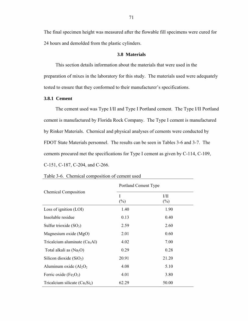
71
The final specimen height was measured after the flowable fill specimens were cured for
24 hours and demolded from the plastic cylinders.
3.8 Materials
This section details information about the materials that were used in the
preparation of mixes in the laboratory for this study. The materials used were adequately
tested to ensure that they conformed to their manufacturer’s specifications.
3.8.1 Cement
The cement used was Type I/II and Type I Portland cement. The Type I/II Portland
cement is manufactured by Florida Rock Company. The Type I cement is manufactured
by Rinker Materials. Chemical and physical analyses of cements were conducted by
FDOT State Materials personnel. The results can be seen in Tables 3-6 and 3-7. The
cements procured met the specifications for Type I cement as given by C-114, C-109,
C-151, C-187, C-204, and C-266.
Table 3-6. Chemical composition of cement used
Portland Cement Type Chemical Composition
I (%)
I/II (%)
Loss of ignition (LOI) 1.40 1.90
Insoluble residue 0.13 0.40
Sulfur trioxide (SO3) 2.59 2.60
Magnesium oxide (MgO) 2.01 0.60
Tricalcium aluminate (Ca3Al) 4.02 7.00
Total alkali as (Na2O) 0.29 0.28
Silicon dioxide (SiO2) 20.91 21.20
Aluminum oxide (Al2O2 4.08 5.10
Ferric oxide (Fe2O3) 4.01 3.80
Tricalcium silicate (Ca3Si2) 62.29 50.00
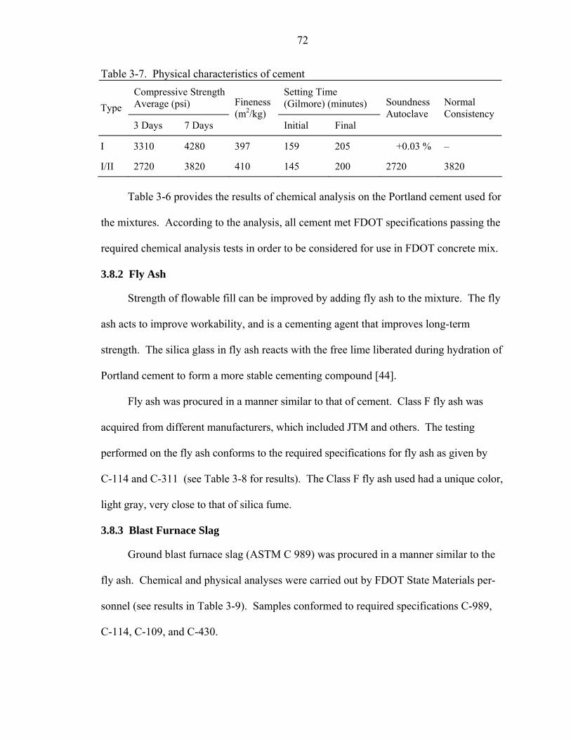
72
Table 3-7. Physical characteristics of cement Compressive Strength Average (psi)
Setting Time (Gilmore) (minutes) Type
3 Days 7 Days
Fineness (m2/kg)
Initial Final
Soundness Autoclave
Normal Consistency
I 3310 4280 397 159 205 +0.03 % –
I/II 2720 3820 410 145 200 2720 3820
Table 3-6 provides the results of chemical analysis on the Portland cement used for
the mixtures. According to the analysis, all cement met FDOT specifications passing the
required chemical analysis tests in order to be considered for use in FDOT concrete mix.
3.8.2 Fly Ash
Strength of flowable fill can be improved by adding fly ash to the mixture. The fly
ash acts to improve workability, and is a cementing agent that improves long-term
strength. The silica glass in fly ash reacts with the free lime liberated during hydration of
Portland cement to form a more stable cementing compound [44].
Fly ash was procured in a manner similar to that of cement. Class F fly ash was
acquired from different manufacturers, which included JTM and others. The testing
performed on the fly ash conforms to the required specifications for fly ash as given by
C-114 and C-311 (see Table 3-8 for results). The Class F fly ash used had a unique color,
light gray, very close to that of silica fume.
3.8.3 Blast Furnace Slag
Ground blast furnace slag (ASTM C 989) was procured in a manner similar to the
fly ash. Chemical and physical analyses were carried out by FDOT State Materials per-
sonnel (see results in Table 3-9). Samples conformed to required specifications C-989,
C-114, C-109, and C-430.

73
Table 3-8. Chemical and physical analyses of fly ash
Parameter Value ASTM C 618 Class F Specifications
Chemical Analysis:
Sum of SiO2, Al2O3, & Fe2O3, % 84.20 min 70.0 Sulfur trioxide (SO3), % 1.00 max 5.0 Moisture content, % 0.10 max 3.0 Loss on ignition, % 4.90 max 6.0 Alkalis as Na2O equivalent, % – max 1.5 Calcium oxide (CaO), % – –
Physical Analysis:
Fineness, amount retained on No. 325 sieve, % 29.00 max 34 Strength activity index–7 days, % 66.00 min 75 Strength activity index–28 days, % 81.00 min 75 Water requirement, % 98.00 max 105 Table 3-9. Chemical and physical analyses of blast furnace slag
Parameter Value ASTM C 989 Grade 100 Specifications
Chemical analysis:
Sulfide sulfur (S), % 0.60 max 2.5 Sulfate ion reported as SO3, % 1.60 max 4.0
Physical analysis:
Fineness, amount retained on No. 325 sieve, % 5.00 max 20 Air content, % – max 12 Slag activity index–7 days, % 108.00 min 90 Slag activity index–28 days, % 142.00 min 110 Specific gravity 2.92 NA 3.8.4 Aggregates
Procurement of aggregates was done in a manner similar to that of the cement.
Table 3-10 provides information concerning the location where fine aggregates were
obtained. The fine aggregate used was silica sand. Throughout the study, two loads of
sand were used. The first load is designated as sand #1 and the second load as sand #2.

74
Table 3-10. Fine aggregate location source Fine Aggregate Type Representative
FDOT District FDOT Approved Aggregate Source Pit No. Location
Silica sand 2 76-349 Melrose, Florida
Both loads came from the same sand mine. Tests on the aggregates were
performed according to ASTM and FDOT specifications. The type of tests performed
included the colorimetric and gradation tests. The colorimetric test was carried out to
provide information on whether the aggregates contain impurities [21]. The tests were
conducted in accordance to AASHTO T21 and AASHTO T71. Impurities interfere with
the process of hydration of cement; coatings would prevent the development of a good
bond between aggregate and the hydrated cement paste as well as other individual
particles which are weak.
The silica sand used in this study varied in color from light gray to sandy white. As
specified by FDOT, the silica sands used were composed of naturally occurring hard,
strong, durable, uncoated grains of quartz and graded from coarse to fine. This type of
sand is the same used for concrete mixes.
3.8.4.1 Aggregate gradation
Gradation is perhaps the most important property of an aggregate. It affects almost
all the important properties for a mix, including the relative aggregate proportions, as
well as the cement and water requirements, workability, pumpability, economy, porosity,
shrinkage, and durability. Therefore, gradation is a primary concern in concrete/flowable
fill mix design. Aggregate gradation is the distribution of particle sizes expressed as a
percent of the total weight. The gradation as a percent of the total volume is also
important, but expressing gradation as a percent by weight is much easier and is a
standard practice. Gradation analyses were performed on all fine aggregates used for all

75
the mixtures created. The gradation was then compared using the ASTM and FDOT’s
upper limit (UL) and lower limit (LL) sieve analysis for fine aggregate as shown below in
Table 3-11. ASTM and FDOT upper/lower limits shall be graded within the limits
indicated in Table 3-11.
Table 3-11. ASTM C33-02A and FDOT specifications for fine aggregate gradation Percent Passing
Sieve Sizes ASTM C33 FDOT
9.50 mm (3/8 in.) 100 100 4.75 mm (No. 4) 95 to 100 95 to 100 2.36 mm (No. 8) 80 to 100 85 to 100 1.18 mm (No. 16) 50 to 85 65 to 97 600 μm (No. 30) 25 to 60 25 to 70 300 μm (No. 50) 5 to 30 5 to 35 75 μm (No. 200) 0 to 10 4
Figure 3-16 illustrates the upper and lower limits of the ASTM C33-02A gradation
for fine aggregates. Figure 3-17 shows the gradation for fine aggregates in accordance
with the FDOT fine aggregates specification. Unlike the ASTM C33-02A higher sieve
0102030405060708090
100
19.1 9.5 2 0.25Sieve Sizes (mm)
Perc
ent P
assi
ng (%
)
ASTM - LL ASTM - UL sand #1 sand #2
Figure 3-16. Gradation of fine aggregates–ASTM specs

76
0102030405060708090
100
19.1 9.5 2 0.25Sieve Sizes (mm)
Perc
ent P
assi
ng (%
)
FDOT - LL FDOT - UL sand #1 sand #2
Figure 3-17. Gradation of fine aggregates–FDOT specs
gradation boundaries, the FDOT higher sieve gradation boundaries allow for both loads
of sand to fall within the required specification gradation limits. Table 3-11 gives fine
aggregate gradation variation that starts from sieve no. 16 down to sieve no. 200 between
ASTM C33-02A and Florida specification.
3.8.4.2 Physical properties, absorption and moisture content
The physical properties for the aggregates were provided by FDOT State Materials
Geotechnical Laboratory. The physical properties for these aggregates are summarized in
Table 3-12.
Table 3-12. Physical properties of fine aggregates (silica sand) Sand #1 Sand #2
Fineness modulus 2.23 2.05 Dry bulk specific gravity 2.63 2.62 Bulk specific gravity (SSD) 2.64 2.63 Apparent specific gravity 2.65 2.65 Absorption — 0.44 — = No data available
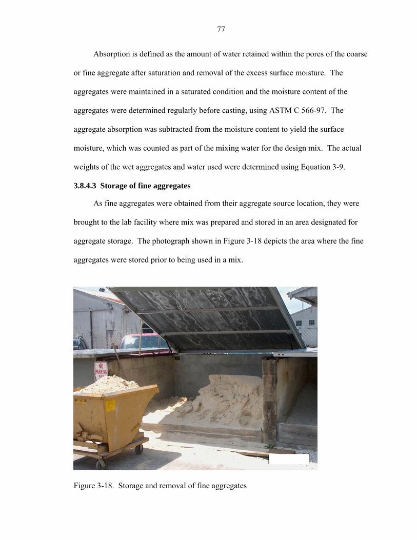
77
Absorption is defined as the amount of water retained within the pores of the coarse
or fine aggregate after saturation and removal of the excess surface moisture. The
aggregates were maintained in a saturated condition and the moisture content of the
aggregates were determined regularly before casting, using ASTM C 566-97. The
aggregate absorption was subtracted from the moisture content to yield the surface
moisture, which was counted as part of the mixing water for the design mix. The actual
weights of the wet aggregates and water used were determined using Equation 3-9.
3.8.4.3 Storage of fine aggregates
As fine aggregates were obtained from their aggregate source location, they were
brought to the lab facility where mix was prepared and stored in an area designated for
aggregate storage. The photograph shown in Figure 3-18 depicts the area where the fine
aggregates were stored prior to being used in a mix.
Figure 3-18. Storage and removal of fine aggregates

78
3.8.5 Admixtures
The admixtures used were air-entraining admixture (AEA). It is classified as a
Darex AEA, and manufactured by W.R. Grace & Co. Darex AEA is a liquid used as an
air-entraining admixture, providing freeze/thaw durability. It contains a catalyst used for
forming a rapid and complete hydration of Portland cement. As it imparts workability
into the mix, Darex AEA is particularly effective with slag, lightweight, or manufactured
aggregates. The AEA used meets all the requirements of ASTM C494.
3.8.6 Water
According to Kosmatka and Panarese, the presence of excessive impurities in
mixing water is known to affect strength and durability of Portland cement concrete (44).
It is believed that concrete and other cementitious mixtures containing mixing water
having high levels of impurities may impact strength development. In this study, potable
water is used as mixing water for production of the flowable fill mixtures.

79
CHAPTER 4 LABORATORY RESULTS AND DISCUSSIONS
4.1 Introduction
This chapter presents the laboratory results of the flowable fill mixtures. The
laboratory tests were conducted at the Florida Department of Transportation State
Materials Office in Gainesville, Florida. Detailed discussions on the results are included,
along with influencing strength factors affecting the long-term behavior of flowable fill.
In Chapter 5, a comprehensive statistical analysis of all data is discussed.
4.2 Laboratory Results
4.2.1 Limerock Bearing Ratio (LBR)
Tables 4-1 and 4-2 provide the LBR results for the mixtures performed in the
laboratory for Experiments 1 and 2. LBR results are shown for 6-hour, 1-, 3-, 28- and
56-day durations. The data shown were found to be repeatable in comparison to their low
coefficient of variation values. From the tables it can be seen that no clear pattern exists
among the individual batch mixes. Statistical analyses of the LBR results are presented
in Chapter 5.
4.2.2 Compressive Strength (psi)
The compressive strength results along with mixture proportions are shown in
Tables 4-3 and 4-4 for each laboratory experiment. Strength results are provided for 1-,
3-, 28- and 56-day durations. Like the LBR data, the compressive strength results were
found to be repeatable. The coefficients of variation for data obtained for both
experiments range from 0% to 45.69%.

80
Table 4-1. LBR strength results for Experiment #1 Batch Mix Number
6-hr Strength (LBR)
Coeff. of Var. (%)
1-day Strength (LBR)
Coeff. of Var. (%)
3-day Strength (LBR)
Coeff. of Var. (%)
28-day Strength (LBR)
Coeff. of Var. (%)
56-day Strength (LBR)
Coeff. of Var. (%)
4 0 -- 1 0.00 10 11.18 52 7.72 49 10.80 25 1 0.00 6 39.74 15 20.96 45 33.68 70 14.50 15 1 0.00 22 47.24 37 19.49 140 12.88 200 19.03 23 3 0.00 14 4.23 34 21.86 148 6.01 223 32.88 50 0 -- 4 15.75 10 11.18 56 14.17 62 6.14 16 0 -- 33 5.25 75 4.81 242 16.36 337 13.50 61 0 -- 1 0.00 3 0.00 17 9.09 15 35.28 34 1 0.00 5 47.30 18 33.71 103 15.59 117 11.35 24 1 0.00 14 21.43 28 8.15 190 13.03 266 22.89 59 0 -- 10 31.11 31 38.21 230 33.90 270 23.76 58 0 -- 2 49.49 12 9.36 77 32.21 81 6.12 51 0 -- 28 32.79 35 9.27 219 44.51 190 4.56 69 0 -- 8 24.98 1 0.00 6 18.23 6 9.12 26 1 0.00 7 37.80 25 0.00 110 14.25 126 8.83 40 1 0.00 23 11.27 42 7.48 142 9.82 118 2.07 16 a 2 0.00 32 0.00 53 9.74 281 11.95 223 4.35 14 1 0.00 13 11.15 28 18.91 90 14.76 80 16.56 8 1 0.00 17 8.81 39 2.56 120 4.41 123 7.79 30 1 0.00 13 12.00 24 23.37 67 14.88 110 26.83 18 1 0.00 8 24.98 21 22.15 81 9.30 99 13.14 20 1 0.00 24 18.79 55 29.22 131 30.27 192 4.45 44 1 0.00 18 3.15 38 4.56 112 5.06 142 8.14 65 0 -- 2 0.00 3 33.33 12 9.90 16 16.54 54 1 0.00 7 7.87 18 5.56 36 30.24 73 28.68 55 0 -- 21 42.01 43 32.81 123 20.74 220 29.16 12 2 0.00 14 8.45 44 30.29 188 7.16 237 4.66 22 1 0.00 4 25.00 12 9.36 60 8.27 81 14.48 33 1 0.00 3 17.32 5 20.00 21 20.76 31 10.48 19 1 11.93 20 12.80 31 11.45 111 3.74 198 34.18 48 0 -- 6 16.67 35 11.66 173 30.65 173 17.67 4a 1 0.00 20 17.27 49 1.19 192 24.02 168 2.98 69a 1 0.00 2 0.00 6 20.38 32 8.27 35 6.54 Note: amixtures batched for a third time due to malfunctions during batching or testing
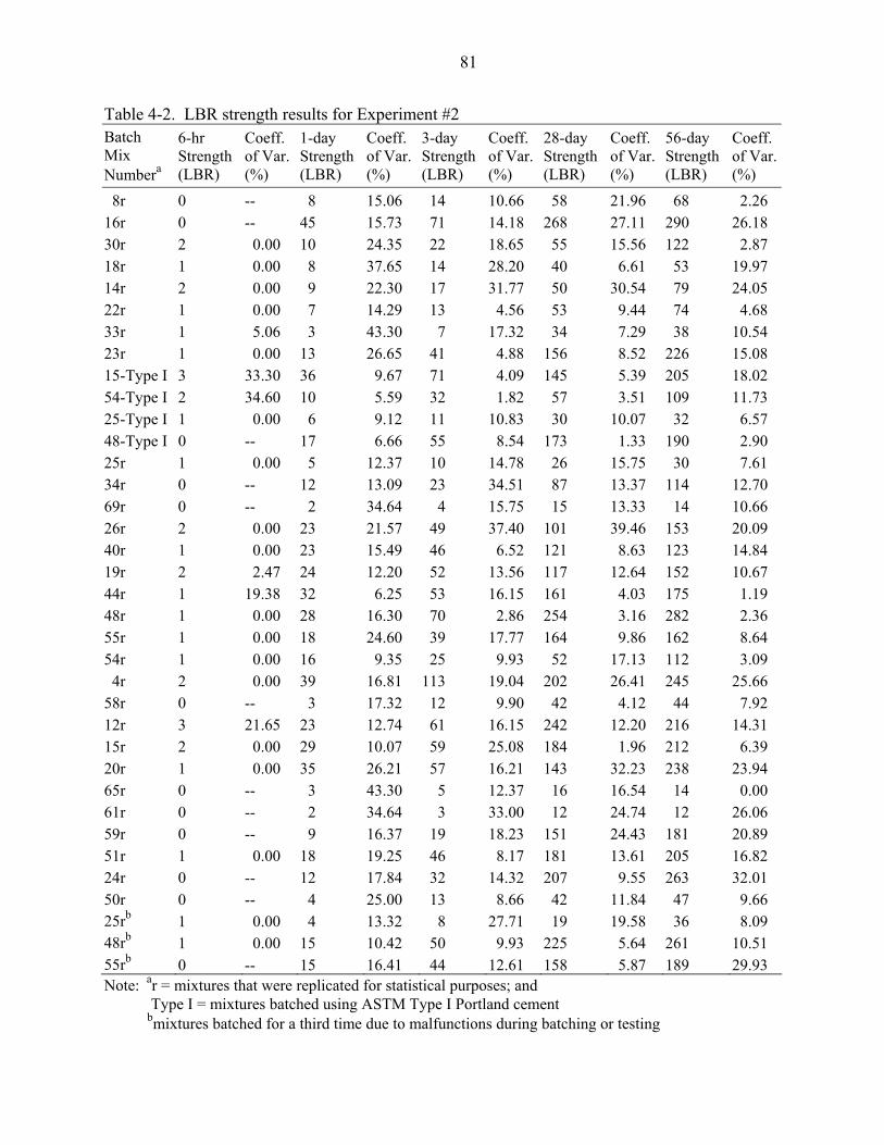
81
Table 4-2. LBR strength results for Experiment #2 Batch Mix Numbera
6-hr Strength (LBR)
Coeff. of Var. (%)
1-day Strength (LBR)
Coeff. of Var. (%)
3-day Strength (LBR)
Coeff. of Var. (%)
28-day Strength (LBR)
Coeff. of Var. (%)
56-day Strength (LBR)
Coeff. of Var.(%)
8r 0 -- 8 15.06 14 10.66 58 21.96 68 2.26 16r 0 -- 45 15.73 71 14.18 268 27.11 290 26.18 30r 2 0.00 10 24.35 22 18.65 55 15.56 122 2.87 18r 1 0.00 8 37.65 14 28.20 40 6.61 53 19.97 14r 2 0.00 9 22.30 17 31.77 50 30.54 79 24.05 22r 1 0.00 7 14.29 13 4.56 53 9.44 74 4.68 33r 1 5.06 3 43.30 7 17.32 34 7.29 38 10.54 23r 1 0.00 13 26.65 41 4.88 156 8.52 226 15.08 15-Type I 3 33.30 36 9.67 71 4.09 145 5.39 205 18.02 54-Type I 2 34.60 10 5.59 32 1.82 57 3.51 109 11.73 25-Type I 1 0.00 6 9.12 11 10.83 30 10.07 32 6.57 48-Type I 0 -- 17 6.66 55 8.54 173 1.33 190 2.90 25r 1 0.00 5 12.37 10 14.78 26 15.75 30 7.61 34r 0 -- 12 13.09 23 34.51 87 13.37 114 12.70 69r 0 -- 2 34.64 4 15.75 15 13.33 14 10.66 26r 2 0.00 23 21.57 49 37.40 101 39.46 153 20.09 40r 1 0.00 23 15.49 46 6.52 121 8.63 123 14.84 19r 2 2.47 24 12.20 52 13.56 117 12.64 152 10.67 44r 1 19.38 32 6.25 53 16.15 161 4.03 175 1.19 48r 1 0.00 28 16.30 70 2.86 254 3.16 282 2.36 55r 1 0.00 18 24.60 39 17.77 164 9.86 162 8.64 54r 1 0.00 16 9.35 25 9.93 52 17.13 112 3.09 4r 2 0.00 39 16.81 113 19.04 202 26.41 245 25.66 58r 0 -- 3 17.32 12 9.90 42 4.12 44 7.92 12r 3 21.65 23 12.74 61 16.15 242 12.20 216 14.31 15r 2 0.00 29 10.07 59 25.08 184 1.96 212 6.39 20r 1 0.00 35 26.21 57 16.21 143 32.23 238 23.94 65r 0 -- 3 43.30 5 12.37 16 16.54 14 0.00 61r 0 -- 2 34.64 3 33.00 12 24.74 12 26.06 59r 0 -- 9 16.37 19 18.23 151 24.43 181 20.89 51r 1 0.00 18 19.25 46 8.17 181 13.61 205 16.82 24r 0 -- 12 17.84 32 14.32 207 9.55 263 32.01 50r 0 -- 4 25.00 13 8.66 42 11.84 47 9.66 25rb 1 0.00 4 13.32 8 27.71 19 19.58 36 8.09 48rb 1 0.00 15 10.42 50 9.93 225 5.64 261 10.51 55rb 0 -- 15 16.41 44 12.61 158 5.87 189 29.93 Note: ar = mixtures that were replicated for statistical purposes; and
Type I = mixtures batched using ASTM Type I Portland cement bmixtures batched for a third time due to malfunctions during batching or testing

82
Table 4-3. Compressive strength results for Experiment #1 Batch Mix Number
1-day Strength (psi)
Coeff. of Var. (%)
3-day Strength (psi)
Coeff. of Var. (%)
28-day Strength (psi)
Coeff. of Var. (%)
56-day Strength (psi)
Coeff. of Var. (%)
4 2 7.90 6 21.19 50 4.23 41 14.69 25 2 0.00 4 24.06 17 15.90 29 5.15 15 4 1.43 13 22.87 58 3.93 93 10.18 23 2 6.38 11 3.81 80 19.56 124 7.74 50 3 4.82 7 7.05 45 9.39 39 3.34 16 6 0.00 19 1.31 89 13.49 133 10.01 61 1 0.00 2 10.59 14 16.26 17 26.19 34 2 3.27 3 35.25 30 14.55 44 9.25 24 2 4.35 8 25.75 79 23.01 155 9.28 59 2 7.16 9 19.32 89 9.03 111 9.02 58 1 3.94 6 6.13 66 5.73 72 6.62 51 2 5.59 15 18.63 67 12.98 108 17.85 69 1 0.00 1 17.84 9 17.78 8 18.39 26 2 0.00 7 0.00 22 0.00 34 15.17 40 10 2.67 32 3.29 138 7.42 114 9.67 16 a 6 0.00 12 0.00 70 7.96 148 7.58 14 2 18.18 8 15.02 58 16.72 69 15.08 8 8 12.08 32 4.76 100 13.40 129 6.02 30 1 18.41 1 0.00 14 22.57 34 18.22 18 2 20.00 5 12.92 33 15.45 43 7.36 20 4 13.12 11 15.84 86 21.76 132 43.98 44 5 25.56 22 5.48 107 1.16 114 9.67 65 1 0.00 1 0.00 3 20.03 8 18.97 54 3 28.67 6 21.31 39 3.80 46 11.64 55 4 7.28 10 0.00 81 2.60 81 38.04 12 13 36.82 34 8.28 143 10.79 139 5.99 22 4 16.22 7 15.15 42 9.38 37 11.47 33 1 15.75 2 27.78 13 11.44 15 14.48 19 5 31.66 16 13.60 56 15.92 132 43.98 48 9 7.84 40 17.95 109 11.96 135 7.77 4a 14 12.70 34 3.25 115 4.09 105 14.86 69a 1 0.00 4 10.26 19 7.77 24 10.88 Note: amixtures batched for a third time due to malfunctions during batching or testing

83
Table 4-4. Compressive strength results for Experiment #2 Batch Mix Numbera
1-day Strength (psi)
Coeff. of Var. (%)
3-day Strength (psi)
Coeff. of Var. (%)
28-day Strength (psi)
Coeff. of Var. (%)
56-day Strength (psi)
Coeff. of Var. (%)
8r 5 13.56 19 9.31 63 3.05 57 4.55 16r 5 0.00 140 15.49 64 2.38 132 16.31 30r 1 18.41 5 43.75 18 27.25 38 23.22 18r 5 6.12 9 20.43 35 6.28 37 5.85 14r 5 8.66 12 12.07 40 11.23 65 12.93 22r 3 12.85 8 17.28 38 34.22 51 9.08 33r 1 17.84 3 1.88 15 10.14 18 8.56 23r 3 13.62 10 17.71 74 7.21 127 18.33 15-Type I 12 1.64 17 15.54 62 20.96 101 13.80 54-Type I 5 29.46 11 13.64 33 6.66 67 45.69 25-Type I 2 5.68 5 11.57 15 24.81 16 6.96 48-Type I 11 7.57 57 22.57 143 1.27 139 5.73 25r 2 15.10 4 16.44 8 0.00 15 8.26 34r 2 3.27 11 31.15 31 12.68 51 18.13 69r 1 0.00 4 23.20 15 18.13 14 20.00 26r 2 0.00 7 0.00 21 7.53 47 33.73 40r 23 9.54 49 10.69 151 2.43 131 0.84 19r 4 15.79 13 0.39 40 7.90 129 32.28 44r 17 8.82 36 10.33 139 5.11 131 0.84 48r 17 8.32 49. 1.42 162 2.47 162 1.80 55r 5 24.51 12. 13.22 53 13.34 98 6.32 54r 6 8.41 10 22.75 33 7.94 56 11.30 4r 30 14.25 63 14.98 159 0.44 161 1.79 58r 2 9.52 7 9.34 43 27.93 41 24.81 12r 19 7.36 32 2.62 137 9.07 143 2.90 15r 13 6.01 19 13.85 66 19.96 136 13.64 20r 16 2.13 15 21.50 92 54.62 129 32.28 65r 2 35.78 2 9.52 5 14.91 10 27.25 61r 1 0.00 2 18.32 10 28.69 11 3.30 59r 2 7.16 8 26.90 97 28.01 99 11.82 51r 2 5.59 18 14.08 102 14.64 170 2.08 24r 2 3.33 8 25.75 57 9.17 125 4.74 50r 3 19.49 10 12.76 36 7.35 44 13.41 25rb 1 7.14 3 28.96 7 17.07 16 9.95 48rb 5 2.96 28 12.17 131 3.49 119 5.58 55rb 4 23.85 14 24.87 49 16.16 100 35.55 Note: ar in mixture number = mixtures that were replicated for statistical purposes; Type I in mixture number = mixes batched using ASTM Type I Portland cement bmixtures batched for a third time due to malfunctions during batching or testing

84
For all the compressive strength samples tested, a load-deflection curve was
created. These curves prove to be useful in helping to determine whether a compressive
strength test went well or not. Viewing each curve, one of the observations made was the
transitional behavior of flowable fill in comparison to soil and concrete. This behavior is
also noted in a study by Folliard et al. In his study, Folliard discussed how flowable fill
demonstrated drastic changes in the deflection curve as the curing time increased. At
early ages, flowable fill acted more like a soil, with it behaving ductile. As time
progressed, the flowable fill behaved more like concrete, with higher strength and low
ductility. This behavior is illustrated in Figure 4-1 for batch mix #4. This behavior was
typical of most flowable fill mixtures.
0
500
1000
1500
2000
2500
0 0.02 0.04 0.06 0.08 0.1 0.12 0.14 0.16
DispIacement (in.)
Load
s (lb
s)
3-day 28-day 56-day
Figure 4-1. Load deformation responses for batch mix #4, at 3-, 28- and 56-day duration
4.2.3 Volume Change
Statistical analysis was used to try to assess which of the three methods provided
reliable data. Using data from the three samples attained per batch mixtures, coefficient

85
of variation was calculated. The coefficient of variation provides a relative measure of
data dispersion compared to the mean. When the coefficient of variation is small, the
data scatter is small compared to the mean. When the coefficient of variation is large
compared to the mean, the amount of variation is large. For example, the variation of
results from methods 1 and 3 ranged from 80% to 95%, whereas, the coefficient of
variation for some specimens using method 2 measured as high as 47.12%. Thus, after
comparing the data from all three methods, the one that produced the most consistent
results and lower variations was method 2. The results for volume change along with
mixture proportions are shown in Tables 4-5 and 4-6. A total of three readings were
taken from each specimen. Those readings were for 1-day, 4-day and 7-day curing
intervals. Data from the 4-day and 7-day readings did not show significant difference
when compared to the 1-day reading. This information demonstrates that much of the
reduction in volume that occurs in flowable fill transpires at its early curing stage or on
the first day.
4.2.4 Proctor Penetrometer Setting Strength (psi)
The proctor penetrometer was used for determining the rate of hardening for
flowable fill mixtures. Tables 4-7 and 4-8 show the test results obtained for the mixtures
tested using the proctor penetrometer. The tables show stress values of all mix samples
for three curing durations. The curing durations are 6 hours, 1 day and 3 days. Appendix
B provides tables containing full detail penetrometer readings for all curing durations.
For those samples designated for testing at 6 hours, the following observations
were noted. At the beginning, since samples were soft, it was not possible to get any
penetrometer readings. However, at a later time, the samples became stiff and
penetrometer readings were obtained. This is due to the fact that flowable fill mixtures

86
Table 4-5. Volume change results for Experiment #1 Batch Mix Number
Cement Content (lb/yd3 )
w/c Ratio
Mineral Admixtures (%)
Target Air Content
Volume Change (%)
Coeff. of Var. (%)
4 200 2.0 0 7.5% ± 2.5% 0.14 0.00 25 50 9.0 0 7.5% ± 2.5% 0.14 33.72 15 150 4.5 0 7.5% ± 2.5% 0.60 0.00 23 150 4.5 50 7.5% ± 2.5% 0.19 42.93 50 100 4.5 0 17.5% ± 2.5% 2.86 0.08 16 200 4.5 0 7.5% ± 2.5% 2.10 0.00 61 50 9.0 0 17.5% ± 2.5% 2.89 8.59 34 100 9.0 50 7.5% ± 2.5% 0.26 5.82 24 200 4.5 50 7.5% ± 2.5% 0.31 37.84 59 150 4.5 50 17.5% ± 2.5% 0.79 4.59 58 100 4.5 50 17.5% ± 2.5% 1.41 9.04 51 150 4.5 0 17.5% ± 2.5% 0.98 3.39 69 50 9.0 50 17.5% ± 2.5% 1.82 26.00 26 100 9.0 0 7.5% ± 2.5% 1.66 2.51 40 200 2.0 0 17.5% ± 2.5% 2.12 10.86 16 a 200 4.5 0 7.5% ± 2.5% 2.10 0.00 14 100 4.5 0 7.5% ± 2.5% 0.35 27.29 8 200 2.0 20 7.5% ± 2.5% 3.11 0.00 30 100 9.0 20 7.5% ± 2.5% 0.16 17.86 18 100 4.5 20 7.5% ± 2.5% 0.57 5.30 20 200 4.5 20 7.5% ± 2.5% 1.38 21.80 44 200 2.0 20 17.5% ± 2.5% 1.33 16.46 65 50 9.0 20 17.5% ± 2.5% 1.39 44.00 54 100 4.5 20 17.5% ± 2.5% 0.52 42.14 55 150 4.5 20 17.5% ± 2.5% 1.06 1.21 12 200 2.0 50 7.5% ± 2.5% 0.29 36.65 22 100 4.5 50 7.5% ± 2.5% 0.54 16.79 33 50 9.0 50 7.5% ± 2.5% 0.46 15.56 19 150 4.5 20 7.5% ± 2.5% 0.38 11.10 48 200 2.0 50 17.5% ± 2.5% 0.54 11.07 4a 200 2.0 0 7.5% ± 2.5% 0.14 0.00 69a 50 9.0 50 17.5% ± 2.5% 1.82 26.00 Note: amixtures batched for a third time due to malfunctions during batching or testing

87
Table 4-6. Volume change results for Experiment #2 Batch Mix Numbera
Cement Content (lb/yd3 )
w/c Ratio
Mineral Admixtures (%)
Target Air Content
Volume Change (%)
Coeff. of Var. (%)
8r 200 2.0 20 7.5% ± 2.5% 3.11 1.61 16r 200 4.5 0 7.5% ± 2.5% 2.10 1.98 30r 100 9.0 20 7.5% ± 2.5% 0.16 17.86 18r 100 4.5 20 7.5% ± 2.5% 0.57 5.30 14r 100 4.5 0 7.5% ± 2.5% 0.35 27.29 22r 100 4.5 50 7.5% ± 2.5% 0.54 16.79 33r 50 9.0 50 7.5% ± 2.5% 0.46 15.56 23r 150 4.5 50 7.5% ± 2.5% 0.19 42.93 15-Type I 150 4.5 0 7.5% ± 2.5% 0.31 22.26 54-Type I 100 4.5 20 17.5% ± 2.5% 0.25 47.12 25-Type I 50 9.0 0 7.5% ± 2.5% 0.89 20.12 48-Type I 200 2.0 50 17.5% ± 2.5% 1.26 24.07 25r 50 9.0 0 7.5% ± 2.5% 0.41 33.72 34r 100 9.0 50 7.5% ± 2.5% 0.26 5.82 69r 50 9.0 50 17.5% ± 2.5% 1.82 26.00 26r 100 9.0 0 7.5% ± 2.5% 1.66 2.51 40r 200 2.0 0 17.5% ± 2.5% 2.12 10.86 19r 150 4.5 20 7.5% ± 2.5% 0.38 11.10 44r 200 2.0 20 17.5% ± 2.5% 1.33 16.46 48r 200 2.0 50 17.5% ± 2.5% 0.54 11.07 55r 150 4.5 20 17.5% ± 2.5% 1.06 1.21 54r 100 4.5 20 17.5% ± 2.5% 0.52 42.14 4r 200 2.0 0 7.5% ± 2.5% 0.14 7.55 58r 100 4.5 50 17.5% ± 2.5% 1.41 9.04 12r 200 2.0 50 7.5% ± 2.5% 0.29 36.65 15r 150 4.5 0 7.5% ± 2.5% 0.60 45.73 20r 200 4.5 20 7.5% ± 2.5% 1.38 21.80 65r 50 9.0 20 17.5% ± 2.5% 1.39 44.00 61r 50 9.0 0 17.5% ± 2.5% 3.89 8.59 59r 150 4.5 50 17.5% ± 2.5% 0.79 4.59 51r 150 4.5 0 17.5% ± 2.5% 0.98 3.39 24r 200 4.5 50 7.5% ± 2.5% 0.31 37.84 50r 100 4.5 0 17.5% ± 2.5% 2.86 9.08 25rb 50 9.0 0 7.5% ± 2.5% 0.17 23.87 48rb 200 2.0 50 17.5% ± 2.5% 0.40 19.88 55rb 150 4.5 20 17.5% ± 2.5% 0.44 4.81 Note: ar in mixture number = mixtures that were replicated for statistical purposes; Type I in mixture number = mixes batched using ASTM Type I Portland cement bmixtures batched for a third time due to malfunctions during batching or testing
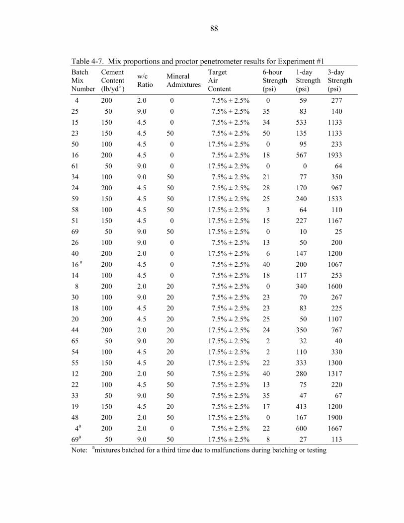
88
Table 4-7. Mix proportions and proctor penetrometer results for Experiment #1 Batch Mix Number
Cement Content (lb/yd3 )
w/c Ratio
Mineral Admixtures
Target Air Content
6-hour Strength (psi)
1-day Strength (psi)
3-day Strength (psi)
4 200 2.0 0 7.5% ± 2.5% 0 59 277 25 50 9.0 0 7.5% ± 2.5% 35 83 140 15 150 4.5 0 7.5% ± 2.5% 34 533 1133 23 150 4.5 50 7.5% ± 2.5% 50 135 1133 50 100 4.5 0 17.5% ± 2.5% 0 95 233 16 200 4.5 0 7.5% ± 2.5% 18 567 1933 61 50 9.0 0 17.5% ± 2.5% 0 0 64 34 100 9.0 50 7.5% ± 2.5% 21 77 350 24 200 4.5 50 7.5% ± 2.5% 28 170 967 59 150 4.5 50 17.5% ± 2.5% 25 240 1533 58 100 4.5 50 17.5% ± 2.5% 3 64 110 51 150 4.5 0 17.5% ± 2.5% 15 227 1167 69 50 9.0 50 17.5% ± 2.5% 0 10 25 26 100 9.0 0 7.5% ± 2.5% 13 50 200 40 200 2.0 0 17.5% ± 2.5% 6 147 1200 16 a 200 4.5 0 7.5% ± 2.5% 40 200 1067 14 100 4.5 0 7.5% ± 2.5% 18 117 253 8 200 2.0 20 7.5% ± 2.5% 0 340 1600 30 100 9.0 20 7.5% ± 2.5% 23 70 267 18 100 4.5 20 7.5% ± 2.5% 23 83 225 20 200 4.5 20 7.5% ± 2.5% 25 50 1107 44 200 2.0 20 17.5% ± 2.5% 24 350 767 65 50 9.0 20 17.5% ± 2.5% 2 32 40 54 100 4.5 20 17.5% ± 2.5% 2 110 330 55 150 4.5 20 17.5% ± 2.5% 22 333 1300 12 200 2.0 50 7.5% ± 2.5% 40 280 1317 22 100 4.5 50 7.5% ± 2.5% 13 75 220 33 50 9.0 50 7.5% ± 2.5% 35 47 67 19 150 4.5 20 7.5% ± 2.5% 17 413 1200 48 200 2.0 50 17.5% ± 2.5% 0 167 1900 4a 200 2.0 0 7.5% ± 2.5% 22 600 1667 69a 50 9.0 50 17.5% ± 2.5% 8 27 113 Note: amixtures batched for a third time due to malfunctions during batching or testing

89
Table 4-8. Mix proportions and proctor penetrometer results for Experiment #2 Batch Mix Numbera
Cement Content (lb/yd3 )
w/c Ratio
Mineral Admixtures
Target Air Content
6-hour Strength (psi)
1-day Strength (psi)
3-day Strength (psi)
8r 200 2.0 20 7.5% ± 2.5% 0 167 510 16r 200 4.5 0 7.5% ± 2.5% 40 583 2133 30r 100 9.0 20 7.5% ± 2.5% 20 77 123 18r 100 4.5 20 7.5% ± 2.5% 5 53 127 14r 100 4.5 0 7.5% ± 2.5% 17 57 160 22r 100 4.5 50 7.5% ± 2.5% 16 77 140 33r 50 9.0 50 7.5% ± 2.5% 17 38 68 23r 150 4.5 50 7.5% ± 2.5% 23 113 900 15-Type I 150 4.5 0 7.5% ± 2.5% 51 427 1567 54-Type I 100 4.5 20 17.5% ± 2.5% 17 153 517 25-Type I 50 9.0 0 7.5% ± 2.5% 16 53 90 48-Type I 200 2.0 50 17.5% ± 2.5% 9 287 1867 25r 50 9.0 0 7.5% ± 2.5% 14 49 102 34r 100 9.0 50 7.5% ± 2.5% 21 127 300 69r 50 9.0 50 17.5% ± 2.5% 0 30 64 26r 100 9.0 0 7.5% ± 2.5% 31 213 390 40r 200 2.0 0 17.5% ± 2.5% 0 633 2467 19r 150 4.5 20 7.5% ± 2.5% 30 500 1247 44r 200 2.0 20 17.5% ± 2.5% 8 455 2000 48r 200 2.0 50 17.5% ± 2.5% 13 420 2600 55r 150 4.5 20 17.5% ± 2.5% 22 202 550 54r 100 4.5 20 17.5% ± 2.5% 12 153 457 4r 200 2.0 0 7.5% ± 2.5% 27 617 2600 58r 100 4.5 50 17.5% ± 2.5% 0 61 177 12r 200 2.0 50 7.5% ± 2.5% 37 317 2067 15r 150 4.5 0 7.5% ± 2.5% 23 327 967 20r 200 4.5 20 7.5% ± 2.5% 24 400 1350 65r 50 9.0 20 17.5% ± 2.5% 0 35 53 61r 50 9.0 0 17.5% ± 2.5% 0 33 54 59r 150 4.5 50 17.5% ± 2.5% 0 60 287 51r 150 4.5 0 17.5% ± 2.5% 19 180 700 24r 200 4.5 50 7.5% ± 2.5% 28 120 517 50r 100 4.5 0 17.5% ± 2.5% 0 95 233 25rb 50 9.0 0 7.5% ± 2.5% 14 49 102 48rb 200 2.0 50 17.5% ± 2.5% 23 324 1250 55rb 150 4.5 20 17.5% ± 2.5% 10 257 425 Note: ar in mixture number = mixtures that were replicated for statistical purposes; Type I in mixture number = mixes batched using ASTM Type I Portland cement bmixtures batched for a third time due to malfunctions during batching or testing

90
are often plastic several hours after mixing. Such observations were noted only for
samples tested after 6 hours of curing.
According to a study by Bhat and Lovell [45], the terminology “walkability” is
used as a criterion for evaluating and comparing hardening characteristics of different
flowable fill mixes. The time required for a particular mix to achieve this strength in
their study is defined as “walkable time” for the mix. The penetration resistance
corresponding to walkability was defined so that walkable time for any mix can be
determined from penetration resistance curves. In the Bhat and Lovell study, the
walkability tests on various flowable fill mixes indicate that the penetration resistance at
that stage varied from 60 to 65 psi depending on the weight of a person. On the basis of
their study results, the walkability time is defined as the time required to achieve a
penetration resistance of 65 psi. This setting time for flowable fill mixture may be used
as a reference for penetration resistance and to determine if the mixture has set. Using
the proctor penetrometer, the penetration resistance was obtained for all samples. From
the results, it can be seen that penetration resistance for all mixtures, at six hours, is well
below the 60 to 65 psi range.
The proctor penetrometer is a great tool to help in ascertaining the field confor-
mance of specifications on flowable fill. The proctor penetrometer is used to measure
penetration resistance of flowable fill. However, it is also a useful tool for strength
measurement up to a certain point in curing time. This was observed while performing
penetrometer resistance tests on 28- and 56-day samples. As hydration proceeded and
flowable fill gained stiffness, the penetrometer exhibited higher values. When samples
became stiff, it became very difficult to penetrate the penetrometer needle into samples at

91
required depth. Between 28 and 56 days, stiffness increased in all samples, and as a
result, the test presented inaccurate results due to the inability of the penetrometer to
penetrate through such strengthened flowable fill. Hence, the penetrometer is a good test
to use in the field where the strength needs to be measured in early setting times to deter-
mine if the flowable fill can support foot traffic and allow further loading. This would
include placement of paving courses for an early opening of traffic, particularly on major
arterials or where heavy volumes of traffic require use of the roadway during rush hour.
4.2.5 Strength Gained Between 28 and 56 Days
To better understand the strength gain between the various intervals of testing, the
percent increase was computed. Figures 4-2 and 4-3 illustrate the percent increase in
strength between 28- and 56-day LBR and compressive strength results. In these
illustrations the w/c ratio is plotted with the percent increased. The hydration of cement
might continue for a long time beyond 28 days. A part of the fly ash and cementitious
materials may be participating in the pozzolanic reaction depending on the nature of the
0.00
5.00
10.00
15.00
20.00
25.00
30.00
2.0 4.5 9.0
w/c ratio
Perc
ent I
ncre
ased
, %
7.5% - air 17.5% - air
Figure 4-2. Percent increase in 56-day strength as compared to 28-day strength (LBR)

92
-10.00
0.00
10.00
20.00
30.00
40.00
2.0 4.5 9.0
w/c ratio
Perc
ent I
ncre
ased
, %
7.5% - air 17.5% - air
Figure 4-3. Percent increase in 56-day strength as compared to 28-day strength (psi)
fly ash [28]. The 56-day strength was as high as 25% or more than the 28-day strength.
On average, there was an increase in 56-day strength with respect to 28-day strength.
As illustrated in Figures 4-2 and 4-3, the mixes with high w/c ratio and low design
air content have a higher percent increase in bearing strength. This behavior can
certainly be explained based on the depletion of water from the mix while curing.
4.2.6 LBR Oven Sample Results
The results of the oven-dried LBR samples give us an exemplary observation of the
role that temperature plays in the curing of flowable fill. As noted earlier, LBR samples
were placed into an oven for 2 days of curing. The oven was set at a temperature of
110° F for the duration of the curing. The average values for the three samples per mix
condition are presented in Tables 4-9 and 4-10. Appendix B contains the individual LBR
values.
A few of the 2-day oven LBR samples tested did not show higher LBR values.
This is because of the hardness of the specimens that caused the LBR machine to

93
Table 4-9. Two-day oven LBR strength results for Experiment #1 Batch Mix Number
Cement Content (lb/yd3 )
w/c Ratio
Mineral Admixtures (%)
Target Air Content
2-day Oven Strength (LBR)
Coeff. of Var. (%)
4 200 2.0 0 7.5% ± 2.5% 33 9.84 25 50 9.0 0 7.5% ± 2.5% 37 20.46 15 150 4.5 0 7.5% ± 2.5% 66 12.03 23 150 4.5 50 7.5% ± 2.5% 74 17.72 50 100 4.5 0 17.5% ± 2.5% 20 5.87 16 200 4.5 0 7.5% ± 2.5% 110 7.22 61 50 9.0 0 17.5% ± 2.5% 7 17.32 34 100 9.0 50 7.5% ± 2.5% 29 14.98 24 200 4.5 50 7.5% ± 2.5% 103 11.93 59 150 4.5 50 17.5% ± 2.5% 82 15.79 58 100 4.5 50 17.5% ± 2.5% 42 11.91 51 150 4.5 0 17.5% ± 2.5% 89 9.60 69 50 9.0 50 17.5% ± 2.5% 1 0.00 26 100 9.0 0 7.5% ± 2.5% 48 34.39 40 200 2.0 0 17.5% ± 2.5% 51 21.39 16 a 200 4.5 0 7.5% ± 2.5% 108 27.82 14 100 4.5 0 7.5% ± 2.5% 61 19.55 8 200 2.0 20 7.5% ± 2.5% 85 45.44 30 100 9.0 20 7.5% ± 2.5% 60 21.67 18 100 4.5 20 7.5% ± 2.5% 37 30.46 20 200 4.5 20 7.5% ± 2.5% 87 18.39 44 200 2.0 20 17.5% ± 2.5% 81 13.02 65 50 9.0 20 17.5% ± 2.5% 9 11.11 54 100 4.5 20 17.5% ± 2.5% 33 13.80 55 150 4.5 20 17.5% ± 2.5% 62 23.38 12 200 2.0 50 7.5% ± 2.5% 145 8.97 22 100 4.5 50 7.5% ± 2.5% 37 9.75 33 50 9.0 50 7.5% ± 2.5% 12 8.33 19 150 4.5 20 7.5% ± 2.5% 62 15.55 48 200 2.0 50 17.5% ± 2.5% 102 10.33 4a 200 2.0 0 7.5% ± 2.5% 101 8.90 69a 50 9.0 50 17.5% ± 2.5% 21 59.67 Note: amixtures batched for a third time due to malfunctions during batching or testing

94
Table 4-10. Two-day oven LBR strength results for Experiment #2 Batch Mix Numbera
Cement Content (lb/yd3 )
w/c Ratio
Mineral Admixtures (%)
Target Air Content
2-day Oven Strength (LBR)
Coeff. of Var. (%)
8r 200 2.0 20 7.5% ± 2.5% 35 7.26 16r 200 4.5 0 7.5% ± 2.5% 126 16.34 30r 100 9.0 20 7.5% ± 2.5% 37 12.89 18r 100 4.5 20 7.5% ± 2.5% 23 15.49 14r 100 4.5 0 7.5% ± 2.5% 32 3.13 22r 100 4.5 50 7.5% ± 2.5% 46 11.89 33r 50 9.0 50 7.5% ± 2.5% 23 6.74 23r 150 4.5 50 7.5% ± 2.5% 186 21.70 15-Type I 150 4.5 0 7.5% ± 2.5% 145 13.08 54-Type I 100 4.5 20 17.5% ± 2.5% 45 8.48 25-Type I 50 9.0 0 7.5% ± 2.5% 20 10.00 48-Type I 200 2.0 50 17.5% ± 2.5% 144 15.58 25r 50 9.0 0 7.5% ± 2.5% 15 6.67 34r 100 9.0 50 7.5% ± 2.5% 79 19.70 69r 50 9.0 50 17.5% ± 2.5% 10 10.00 26r 100 9.0 0 7.5% ± 2.5% 56 11.55 40r 200 2.0 0 17.5% ± 2.5% 60 3.33 19r 150 4.5 20 7.5% ± 2.5% 106 40.71 44r 200 2.0 20 17.5% ± 2.5% 133 1.99 48r 200 2.0 50 17.5% ± 2.5% 242 3.16 55r 150 4.5 20 17.5% ± 2.5% 93 18.72 54r 100 4.5 20 17.5% ± 2.5% 57 17.28 4r 200 2.0 0 7.5% ± 2.5% 174 10.64 58r 100 4.5 50 17.5% ± 2.5% 67 9.55 12r 200 2.0 50 7.5% ± 2.5% 197 5.14 15r 150 4.5 0 7.5% ± 2.5% 107 23.80 20r 200 4.5 20 7.5% ± 2.5% 108 11.60 65r 50 9.0 20 17.5% ± 2.5% 11 23.59 61r 50 9.0 0 17.5% ± 2.5% 4 13.32 59r 150 4.5 50 17.5% ± 2.5% 136 20.23 51r 150 4.5 0 17.5% ± 2.5% 94 21.42 24r 200 4.5 50 7.5% ± 2.5% 60 26.59 50r 100 4.5 0 17.5% ± 2.5% 45 7.09 25rb 50 9.0 0 7.5% ± 2.5% 12 25.00 48rb 200 2.0 50 17.5% ± 2.5% 232 3.95 55rb 150 4.5 20 17.5% ± 2.5% 129 15.20 Note: ar in mixture number = mixtures that were replicated for statistical purposes; Type I in mixture number = mixes batched using ASTM Type I Portland cement bmixtures batched for a third time due to malfunctions during batching or testing

95
terminate itself. Some of the specimen LBR plots show the LBR values going up and
then coming down and then going up again. This peculiar behavior was observed for
many of the samples containing fly ash, slag and high cement content. Many of the
samples demonstrating the aforementioned behavior showed signs of fracture and
cracking when the LBR test was performed.
Table 4-11 provides comparison of mixture components and their influence on
accelerated 2-day oven and 28-day LBR strength. The table shows mixtures with a low
w/c ratio exhibit a high accelerated strength. This demonstrates the heat of hydration
occurring fully due to the oven temperature, which acts as a catalyst to speed up curing.
Table 4-11. Comparison of mixture components and their influence on accelerated 2-day oven and 28-day LBR strength
Design Air Content (%)
W/C Ratio
2-day Oven Strength (LBR)
28-day Oven Strength (LBR)
2.0 99 142 4.5 81 133 7.5 9.0 40 65 2.0 95 147 4.5 67 115 17.5 9.0 10 16
Design Air Content (%)
Mineral Admixtures (%)
2-day Oven Strength (LBR)
28-day Oven Strength (LBR)
0% 68 123 20% - fly ash 64 92
7.5 50% - slag 83 124
0% 46 99 20% - fly ash 58 85
17.5 50% - slag 75 111 Design Air Content (%)
Cement Content (lbs/yd3 )
2-day Oven Strength (LBR)
28-day Oven Strength (LBR)
50 17 16 100 45 75 150 107 136
7.5
200 98 171 50 10 16 100 42 51 150 93 178
17.5
200 95 147

96
4.3 Factors Affecting Strength
4.3.1 Water-to-Cement (w/c) Ratio
Strength, because it can easily be determined, is the most universally used measure
for flowable fill quality. Like concrete, the compressive strength is inversely related to
the water/cement (w/c) ratio. To identify this relationship, plots of w/c ratio versus
strength were created. The relationship between strength and w/c ratio for two levels of
air content are shown in Figures 4-4 through 4-7. It is common knowledge among
0.00
50.00
100.00
150.00
200.00
250.00
300.00
0.0 2.0 4.0 6.0 8.0 10.0
w/c ratio
Stre
ngth
, LB
R
design air content 7.5%
Figure 4-4. Relationship between 28-day bearing strength (LBR) and w/c ratio at 7.5%
design air content
0.00
50.00
100.00
150.00
200.00
250.00
300.00
0.0 2.0 4.0 6.0 8.0 10.0w/c ratio
Stre
ngth
, LB
R
design air content 17.5%
Figure 4-5. Relationship between 28-day bearing strength (LBR) and w/c ratio at 17.5%
design air content

97
0.00
50.00
100.00
150.00
200.00
0.0 2.0 4.0 6.0 8.0 10.0w/c ratio
Stre
ngth
, psi
design air content 7.5%
Figure 4-6. Relationship between 28-day compressive strength (psi) and w/c ratio at
7.5% design air content
0.00
50.00
100.00
150.00
200.00
0.0 2.0 4.0 6.0 8.0 10.0w/c ratio
Stre
ngth
, psi
design air content 17.5%
Figure 4-7. Relationship between 28-day compressive strength (psi) and w/c ratio at
17.5% design air content
engineers that the strength, like other desirable properties of flowable fill under given job
conditions, is governed by the quantity of mixing water used per unit of cement. Thus,
the ratio of water to cementitious material has a major influence on the strength of flow-
able fill. For the plots in Figures 4-4 through 4-7, this relationship is evident between the
w/c ratio and strength. Since w/c ratio primarily controls strength, it is expected that
strength decreases as the amount of water increases. The plots illustrate that as the w/c
ratio increases, strength decreases. Although a particular w/c ratio is specified in
designing a mix, there is often a great deal of uncertainty over what the true w/c ratio is
when the mix is actually placed.

98
4.3.2 Cement Content
Cement content is an important factor in determining bearing strength. The plots in
Figures 4-8 through 4-13 indicate the strength in relation to cement content for air-
entrained mixtures (7.5% and 17.5 %) by design. Just like w/c ratio, one expects strength
to increase with increasing cement content. This normally occurs for mixtures containing
normal workability. This is apparent with plots showing the relations of strength with
cement content. The plots indicate that mixes with higher cement content exhibit higher
strength for both LBR and compressive strength samples.
0.0050.00
100.00150.00200.00250.00300.00
0.0 50.0 100.0 150.0 200.0 250.0cement content, lb/yd3
Stre
ngth
, LB
R
design air content 7.5%
Figure 4-8. Relationship between 28-day bearing strength (LBR) and cement content at
7.5% design air content
0.00
50.00
100.00
150.00
200.00
250.00
300.00
0.0 50.0 100.0 150.0 200.0 250.0cement content, lb/yd3
Stre
ngth
, LB
R
design air content 17.5%
Figure 4-9. Relationship between 28-day bearing strength (LBR) and cement content at 17.5% design air content

99
Figure 4-10. Relationship between 28-day compressive strength (psi) and cement content
at 7.5% design air content
0.00
50.00
100.00
150.00
200.00
0.0 50.0 100.0 150.0 200.0 250.0cement content, lb/yd3
Stre
ngth
, psi
design air content 17.5%
Figure 4-11. Relationship between 28-day compressive strength (psi) and cement content at 17.5% design air content
Figure 4-12. Relationship between 28-day LBR strength and cement content
0.00
50.00
100.00
150.00
200.00
0.0 50.0 100.0 150.0 200.0 250.0
cement content, lb/yd3
Stre
ngth
, psi
design air content 7.5%
0.0050.00
100.00150.00200.00250.00
0 50 100 150 200 250cement content, lb/yd3
Stre
ngth
, LB
R
7.5% - air 17.5% - airdesign air content 7.5% design air content 17.5%
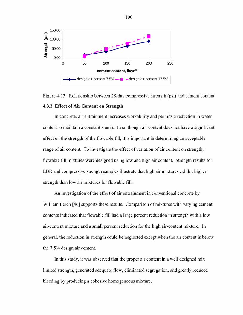
100
Figure 4-13. Relationship between 28-day compressive strength (psi) and cement content
4.3.3 Effect of Air Content on Strength
In concrete, air entrainment increases workability and permits a reduction in water
content to maintain a constant slump. Even though air content does not have a significant
effect on the strength of the flowable fill, it is important in determining an acceptable
range of air content. To investigate the effect of variation of air content on strength,
flowable fill mixtures were designed using low and high air content. Strength results for
LBR and compressive strength samples illustrate that high air mixtures exhibit higher
strength than low air mixtures for flowable fill.
An investigation of the effect of air entrainment in conventional concrete by
William Lerch [46] supports these results. Comparison of mixtures with varying cement
contents indicated that flowable fill had a large percent reduction in strength with a low
air-content mixture and a small percent reduction for the high air-content mixture. In
general, the reduction in strength could be neglected except when the air content is below
the 7.5% design air content.
In this study, it was observed that the proper air content in a well designed mix
limited strength, generated adequate flow, eliminated segregation, and greatly reduced
bleeding by producing a cohesive homogeneous mixture.
0.00
50.00
100.00
150.00
0 50 100 150 200 250
cement content, lb/yd3
Stre
ngth
(psi
)
7.5% - air 17.5% - airdesign air content 7.5% design air content 17.5%
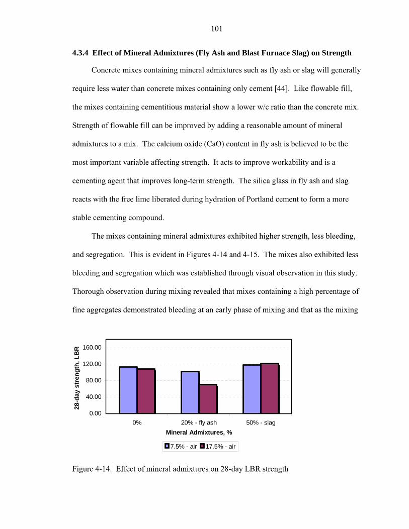
101
4.3.4 Effect of Mineral Admixtures (Fly Ash and Blast Furnace Slag) on Strength
Concrete mixes containing mineral admixtures such as fly ash or slag will generally
require less water than concrete mixes containing only cement [44]. Like flowable fill,
the mixes containing cementitious material show a lower w/c ratio than the concrete mix.
Strength of flowable fill can be improved by adding a reasonable amount of mineral
admixtures to a mix. The calcium oxide (CaO) content in fly ash is believed to be the
most important variable affecting strength. It acts to improve workability and is a
cementing agent that improves long-term strength. The silica glass in fly ash and slag
reacts with the free lime liberated during hydration of Portland cement to form a more
stable cementing compound.
The mixes containing mineral admixtures exhibited higher strength, less bleeding,
and segregation. This is evident in Figures 4-14 and 4-15. The mixes also exhibited less
bleeding and segregation which was established through visual observation in this study.
Thorough observation during mixing revealed that mixes containing a high percentage of
fine aggregates demonstrated bleeding at an early phase of mixing and that as the mixing
0.00
40.00
80.00
120.00
160.00
0% 20% - fly ash 50% - slagMineral Admixtures, %
28-d
ay s
tren
gth,
LB
R
7.5% - air 17.5% - air
Figure 4-14. Effect of mineral admixtures on 28-day LBR strength

102
0.00
50.00
100.00
150.00
200.00
0% 20% - fly ash 50% - slagMineral Admixtures, %
56-d
ay s
tren
gth,
LB
R
7.5% - air 17.5% - air
Figure 4-15. Effect of mineral admixtures on 56-day LBR strength
was prolonged, the bleeding slowed. This phenomenon exhibited in mixes containing
zero mineral admixtures. Excessive bleeding often indicates a bad mix. This type of mix
should be avoided in the field due to the possibility of the mix not having good flow. In
addition, such a mix may result in excessive initial subsidence of the surface after
placement.
4.4 Comparison of Mix Using Type I/II Cement vs. Type I Cement
During the research experiment, it was discovered that certain mixtures utilized
Type I cement as opposed to Type I/II cement obtained for the research project. When
this was discovered, additional mixture was prepared using strictly Type I cement. The
compressive and LBR strength results were then compared to similar mixtures where
Type I/II cement was used. Figures 4-16 through 4-23 shown below are plots of the
comparison of both LBR and psi compressive strengths for four mixes.
The four mixtures chosen included both high and low cement content. Based on
the results obtained for those mixtures, it was concluded that the difference in strength
between the two types of cement was not significant.
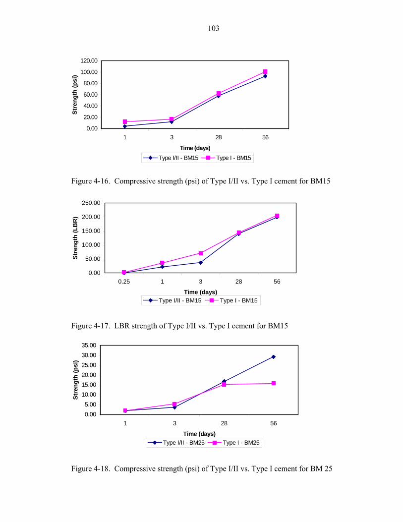
103
0.00
20.00
40.00
60.00
80.00
100.00
120.00
1 3 28 56
Time (days)
Stre
ngth
(psi
)
Type I/II - BM15 Type I - BM15
Figure 4-16. Compressive strength (psi) of Type I/II vs. Type I cement for BM15
0.00
50.00
100.00
150.00
200.00
250.00
0.25 1 3 28 56
Time (days)
Stre
ngth
(LB
R)
Type I/II - BM15 Type I - BM15
Figure 4-17. LBR strength of Type I/II vs. Type I cement for BM15
0.005.00
10.0015.0020.0025.0030.0035.00
1 3 28 56
Time (days)
Stre
ngth
(psi
)
Type I/II - BM25 Type I - BM25
Figure 4-18. Compressive strength (psi) of Type I/II vs. Type I cement for BM 25

104
0.00
5.00
10.00
15.00
20.00
25.00
30.00
35.00
0.25 1 3 28 56
Time (days)
Stre
ngth
(LB
R)
Type I/II - BM25 Type I - BM25
Figure 4-19. LBR strength of Type I/II vs. Type I cement for BM 25
0.0020.0040.0060.0080.00
100.00120.00140.00160.00
1 3 28 56
Time (days)
Stre
ngth
(psi
)
Type I/II - BM48 Type I - BM48
Figure 4-20. Compressive strength (psi) of Type I/II vs. Type I cement for BM 48
0.00
40.00
80.00
120.00
160.00
200.00
0.25 1 3 28 56
Time (days)
Stre
ngth
(LB
R)
Type I/II - BM48 Type I - BM48
Figure 4-21. LBR strength of Type I/II vs. Type I cement for BM 48

105
0.00
10.00
20.00
30.00
40.00
50.00
60.00
70.00
1 3 28 56
Time (days)
Stre
ngth
(psi
)
Type I/II - BM54 Type I - BM54
Figure 4-22. Compressive strength (psi) of Type I/II vs. Type I cement for BM 54
0.00
20.00
40.00
60.00
80.00
100.00
120.00
0.25 1 3 28 56
Time (days)
Stre
ngth
(LB
R)
Type I/II - BM54 Type I - BM54 Figure 4-23. LBR strength of Type I/II vs. Type I cement for BM 54
4.5 Drying Shrinkage (Volume Change)
Based on the results obtained, it was determined that the word “shrinkage” was not
appropriate terminology to describe the occurrence of settlement in flowable fill. Instead,
the term “volume change” was adopted to describe drying shrinkage in flowable fill.
The occurrence of volume change in flowable fill under service conditions arises
from a number of different stimuli. Some of these stimuli are applied stress, change in
moisture content, and changes in temperature. The plots below illustrate the effected
volume change in flowable fill due to w/c ratio, cement content, and mineral admixtures.

106
Table 4-12 shows a comparison of mixture components and their influence on
percent volume change. In Figure 4-24, the effect of the w/c ratio on the change in
volume in flowable fill indicates that volume change increases with increased w/c ratio
for mixtures with high air-content, while the change in volume for mixes with low air-
content is minimal and does not appear to be significant.
Table 4-12. Comparison of mixture components and their influence on percent volume change
Design Air Content (%)
W/C Ratio
Volume Change (%)
2.0 1.18 4.5 0.71 7.5 9.0 0.59 2.0 1.33 4.5 1.27 17.5 9.0 2.37
Design Air Content (%) Mineral Admixtures Volume Change
(%) 0% 0.88 20% - fly ash 1.12 7.5 50% - slag 0.34 0% 2.47 20% - fly ash 1.07 17.5 50% - slag 1.14
Design Air Content (%)
Cement Content (lbs/yd3 )
Volume Change (%)
50 0.43 100 0.59 150 0.39
7.5
200 1.22 50 2.37 100 1.60 150 0.94
17.5
200 1.33
The effect of cement content on flowable fill volume change seems to have an
effect opposite of that of the w/c ratio as illustrated in Figure 4-25.
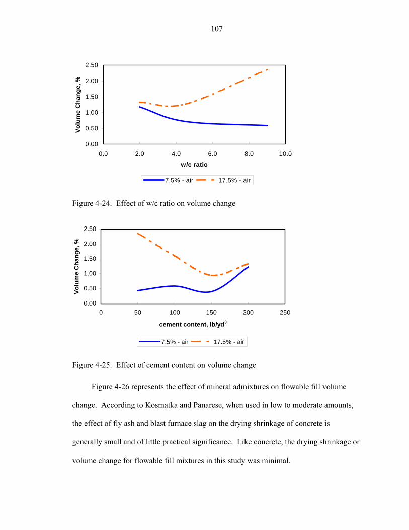
107
0.00
0.50
1.00
1.50
2.00
2.50
0.0 2.0 4.0 6.0 8.0 10.0
w/c ratio
Volu
me
Cha
nge,
%
7.5% - air 17.5% - air
Figure 4-24. Effect of w/c ratio on volume change
0.00
0.50
1.00
1.50
2.00
2.50
0 50 100 150 200 250
cement content, lb/yd3
Volu
me
Cha
nge,
%
7.5% - air 17.5% - air
Figure 4-25. Effect of cement content on volume change
Figure 4-26 represents the effect of mineral admixtures on flowable fill volume
change. According to Kosmatka and Panarese, when used in low to moderate amounts,
the effect of fly ash and blast furnace slag on the drying shrinkage of concrete is
generally small and of little practical significance. Like concrete, the drying shrinkage or
volume change for flowable fill mixtures in this study was minimal.

108
0.00
0.50
1.00
1.50
2.00
2.50
3.00
0% 20% - fly ash 50% - slag
Mineral Admixtures, %
Volu
me
Cha
nge,
%
7.5% - air 17.5% - air
Figure 4-26. Effect of mineral admixtures on volume change
4.6 Interpretation of Plastic Test Results
Tests for plastic properties were performed at the end of every batch mix. The
characteristics measured were unit weight, air content, flow consistency, and temperature.
Tables 3-3 and 3-4 in Chapter 3 give the outcome of the plastic tests performed.
The unit weights for flowable fill mixtures in this study ranged from 99.92 to
137.28 lb/ft3. In comparison to normal concrete mixtures, the unit weight for air-
entrained flowable fill mixtures was slightly less than those of normal concrete mixtures.
Air content was measured using the pressure method. This method was found to be
simple and reliable. The measuring instrument used was a calibrated pressure meter.
The mixtures used in this study were designed using a low air-content target (7.5±2.5%)
and a high air-content target (17.5± 2.5%). At the time of batching, care was taken to
ensure that the target air content was achieved. It was extremely difficult to obtain the
entrained air target for mixtures with very low sand-to-water ratio or certain stiff
mixtures. For example, during the batching of batch mix #16 there was a problem in
obtaining the target air content (7.5% ± 2.5%). After several attempts were made to

109
reach the target air content, the only attainable air content was established at 1.3%.
Below is the amount of air entraining admixture (AEA) added on each of the attempts
and the resulting air content:
• Attempt 1: AEA _ 100 ml, 0.5% air • Attempt 2: AEA 100 ml, 1.0% air; and • Attempt 3: AEA _ 1400 ml, 1.3% air.
After adding the AEA to the mix, the mixer was rotated for seven to ten minutes. It
was observed that the mix had foam or air bubbles forming on the surface of mix. This
was an indication that the air was difficult to retain in the mix, due to the fluidity of the
mix (sand-to-water ratio = 1.74). It is believed that mixtures containing high water
content prevents the formation of entrained air voids, which thus rendered the AEA to be
noneffective. For various mixtures, air-entraining dosage rates were increased to the
dosage recommended by the manufacturer, but to no avail, the target air contents were
not achieved.
The flow consistency was measured in accordance to ASTM D 6103 test
procedures. ASTM D 6103 requires the implementation of an open-ended flow cylinder
that is 150 mm (6 in.) in length and has a 76 mm (3 in.) inside diameter. The flow
cylinder used throughout this experiment was made of PVC. Once the flowable fill had
been properly mixed, the material was placed into one end of the cylinder, while the other
rested on a flat wet surface. Both the flow cylinder and flat surface were dampened with
water prior to testing. After a few seconds of filling the cylinder, it was quickly and
carefully raised in the vertical direction. The largest resulting spread diameter was then
immediately measured using a ruler by taking the average of two perpendicular
measurements.

110
For a flowable fill to be self-leveling and ready for use in filling void spaces with-
out requiring vibration, the average spread diameter should be between 8 and 12 in. [45].
This type of spread is also known to provide suitable flow during placement of flowable
fill in the field. Flow values in Tables 3-3 and 3-4 ranged from 0.00 to 10.50 in.
Figure 4-27 is a bar chart plotting the sand-to-water ratio versus the flow diameter.
To understand the behavior of one class of mixtures having high flow and the other class
having less flow, it is critical to understand the behavior of different material ingredients
in the flowable fill. Water, for example, is expected to be the key ingredient responsible
for flow. Looking at the water/cement (w/c) ratio per mixtures, however, it shows that
most of the mixes with low-flow spread are those that contain a high w/c ratio. The
differences in flowability can be attributed to the amounts of mineral admixtures that a
mix contains.
0.00
2.00
4.00
6.00
8.00
10.00
12.00
1.73
1.74
1.83
2.59
2.60
3.25
5.30
5.31
5.40
6.06
6.09
6.29
6.38
7.17
7.20
s/w ratio
Flow
dia
met
er, i
n.
Figure 4-27. Flow diameter vs. sand-to-water ratio

111
CHAPTER 5 STATISTICAL ANALYSIS
5.1 Introduction
One of the objectives of this study was to develop predictive models for strength
and volume change of flowable fill. This section details the statistical approaches and the
statistical derivation of the linear regression equations that resulted in the assessment of
the statistical models.
5.2 Statistical Model Derivation
Multiple linear regression analysis is the multivariate method used for analyzing
the laboratory data obtained in this study. Regression analyses are defined as a set of
statistical procedures for assessing the relationship between one random variable and
several fixed independent variables [40]. In this data analysis, the strength (i.e., LBR and
compressive) and shrinkage (volume change) were the dependent variables, while cement
content, air content, w/c ratio, and mineral admixtures were the independent variables
(also referred to as explanatory variables). A simple mathematical regression equation is
generally represented by
( , )y f x b ε= + (5-1)
where y is the dependent variable, b contains the regression parameters, x is a set of
independent variables, and ε is the random error of the estimated function. The ordinary
least squares method was applied for estimating the regression parameters. The least
squares method minimizes the sum of squares of the differences between the predicted

112
and the actual values of the dependent variable. Using the least squares method takes
into account the following assumptions:
1. Stability of the regression model. This implies that the value of the dependent variable y is an additive combination of the independent predictor variables represented as x. Theoretically, if there is an interaction effect such that the value of one explanatory variable depends on one or more other explanatory variables, the estimates of the regression coefficients are statistically unreliable.
2. Constancy of error variance. It is assumed that the error term (ε) is not correlated with the independent variables and assumes constant variability over the range of the variables. The dependent variable, y, is also assumed to have a constant variance. This entails that the dependent variables are independent of each other.
3. Normality of the response variable, y. The normality of regression formulation is usually assessed through normality residual plots.
4. Normality of the error terms, ε. The least squares approach for estimating regression parameters is most efficient when the residuals or errors also have a normal probability distribution.
In summary, the validity of a multiple regression model uses the classical assump-
tions described above. Those assumptions are linearity, independency and normality.
To satisfy the basic assumptions, it is customary to apply various remedies and
diagnostics for individual variables. Some of these remedies involve transformation.
Transformation or re-expression of the response is the primary tool for dealing with
violations of assumptions. For example, the logarithm of the response might be analyzed.
The idea is that the responses on the transformed scale match our assumptions more
closely, so that we can use standard methods on the transformed data. In simple terms,
transformation of variables is necessary so as to simplify or straighten relationships,
stabilize variances, and improve normality [41]. For this study, some of the explanatory
variables had a nonlinear trend with the values of the strength and volume change. For
example, cement content had a curvilinear relationship with the value of the response
variables, so a quadratic term relating to the cement content was used to convert the

113
nonlinear relationship into a linear one. Similarly, the data interpretation showed that the
w/c ratio had a nonlinear relationship with the response variable and the relationship was
straightened by a transformation on its variable.
When the classical assumptions of constant variance and normality are violated, a
nonlinear transformation of the response may improve the regression fit. Evaluation of
the data revealed normal distributions of the residuals, indicating that no transformation
was necessary to satisfy this assumption [41].
When the effects of the independent variables on the response variable are not
additive, the effect of one independent variable depends on the levels of the other
predictor variables [40]. In this study, the polynomial regression models required to
simplify the relationships between strength (i.e., LBR, compressive) and volume change
contained interaction effects, resulting in non-constant variance. A simple and
commonly used means of modeling the interaction effect of two predictor variables on
the response variable is by a cross-product term called an “interaction term” [40].
Consequently, the interaction terms for all explanatory variables were included in the
regression equations.
After considering the potential regression problems and taking their remedies,
regression models were generated using ordinary least squares method. Because the
independent variables were reasonably orthogonal, ordinary least squares results
remained almost the same regardless of which other variables were included in the
model. All possible subset regressions were computed and evaluated to provide the best
statistical model. This method was feasible because the number of independent variables
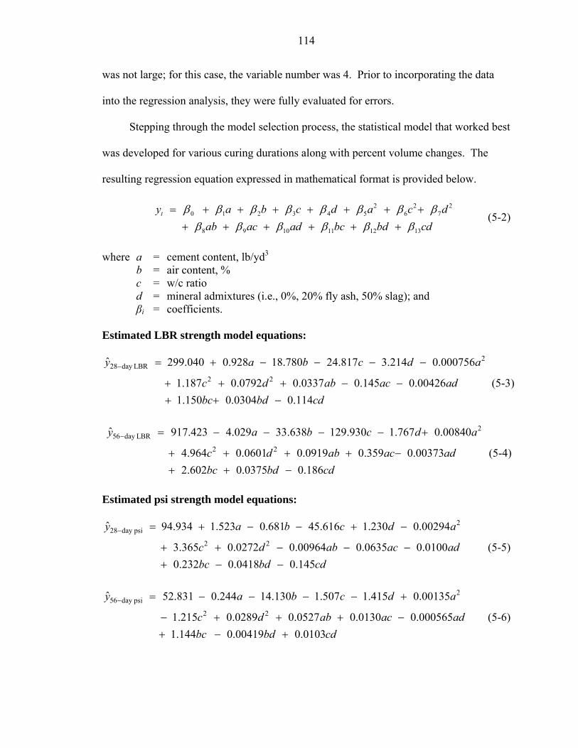
114
was not large; for this case, the variable number was 4. Prior to incorporating the data
into the regression analysis, they were fully evaluated for errors.
Stepping through the model selection process, the statistical model that worked best
was developed for various curing durations along with percent volume changes. The
resulting regression equation expressed in mathematical format is provided below.
2 2 2
0 1 2 3 4 5 6 7
8 9 10 11 12 13
ty a b c d a c dab ac ad bc bd cd
β β β β β β β ββ β β β β β
= + + + + + + ++ + + + + +
(5-2)
where a = cement content, lb/yd3 b = air content, % c = w/c ratio d = mineral admixtures (i.e., 0%, 20% fly ash, 50% slag); and βi = coefficients. Estimated LBR strength model equations:
228 day LBR
2 2
ˆ 299.040 0.928 18.780 24.817 3.214 0.000756
1.187 0.0792 0.0337 0.145 0.004261.150 0.0304 0.114
y a b c d a
c d ab ac adbc bd cd
− = + − − − −
+ + + − −+ + −
(5-3)
256 day LBR
2 2
ˆ 917.423 4.029 33.638 129.930 1.767 0.00840
4.964 0.0601 0.0919 0.359 0.003732.602 0.0375 0.186
y a b c d a
c d ab ac adbc bd cd
− = − − − − +
+ + + + −+ + −
(5-4)
Estimated psi strength model equations:
228 day psi
2 2
ˆ 94.934 1.523 0.681 45.616 1.230 0.00294
3.365 0.0272 0.00964 0.0635 0.01000.232 0.0418 0.145
y a b c d a
c d ab ac adbc bd cd
− = + − − + −
+ + − − −+ − −
(5-5)
256 day psi
2 2
ˆ 52.831 0.244 14.130 1.507 1.415 0.00135
1.215 0.0289 0.0527 0.0130 0.0005651.144 0.00419 0.0103
y a b c d a
c d ab ac adbc bd cd
− = − − − − +
− + + + −+ − +
(5-6)

115
Estimated percent volume change model equations:
% volume change
2 2 2
ˆ 3.945 0.00457 0.193 0.667 0.0284
0.0000105 0.0373 0.000185 0.0001160.00904 0.0000700 0.0128 0.0001650.00445
y a b c d
a c d abac ad bc bdcd
= − − + − +
+ + − −+ − + −−
(5-7)
The mathematical equations shown above represent the regression model equations
for estimating the LBR strength, compressive strength in psi, as well as the volume
change. Table 5-1 provides the standard errors and other pertinent information for each
regression model equation.
The accuracy of the fitted data for each regression model can be better understood
by inspection of Figures 5-1 through 5-3. These figures plot the fitted versus the
standardized residuals. For Figures 5-1 and 5-2, it is clear that both plots show a right-
opening megaphone shape. This clearly indicates that variability of the residuals
increased with response mean. The conclusions drawn from these graphs were that the
fitted values provided a reasonable estimate of the actual values and the regression
models could be useful for designing a flowable fill mixture. The residuals plot in Figure
5-3 does not provide a clear megaphone shape as in Figures 5-1 and 5-2, thus it was
difficult to determine whether or not the residuals increased with the response mean. The
results of analysis of variance are provided in Appendix C. Appendix C contains the
parameters and standard error for each regression equation along with tables and figures
displaying the comparison of measured laboratory and predicted results. The results
showed highly significant differences between some independent variables for all
models. The multiple correlation coefficients (R-square) were 0.846 for 28-day LBR and
0.853 for 56-day LBR.

116
Table 5-1. Standard error of regression coefficients for equations relating mixture constituents to LBR, compressive strength and percent volume change
Equation Models Coefficient (βi ) y28–day LBR y56–day LBR y28–day psi y56–day psi y% volume change
β0 = 549.872 624.940 278.578 341.164 1.403 β1 = 3.740 4.250 1.895 2.320 0.00954 β2 = 12.536 14.248 6.351 7.778 0.0320 β3 = 111.985 127.273 56.734 69.480 0.286 β4 = 1.847 2.100 0.936 1.146 0.00472 β5 = 0.00630 0.00716 0.00319 0.00391 0.0000161 β6 = 5.165 5.870 2.617 3.205 0.0132 β7 = 0.00915 0.0104 0.00464 0.00568 0.0000234 β8 = 0.0524 0.0595 0.0265 0.0325 0.000134 β9 = 0.392 0.445 0.199 0.243 0.00100 β10 = 0.00658 0.00748 0.00334 0.00408 0.0000168 β11 = 1.325 1.506 0.671 0.822 0.00338 β12 = 0.0278 0.0316 0.0141 0.0172 0.0000709 β13 = 0.129 0.147 0.0653 0.0800 0.000329 R-Square 0.846 0.853 0.880 0.859 0.569 MSE 986.578 1274.340 253.223 379.783 0.00643 DFE 159.00 159.00 159.00 159.00 159.00 COV 27.718 25.822 25.767 24.210 62.228
Figure 5-1. Residuals versus fitted values plot (28-day LBR)
Stan
dard
ized
Res
idua
l
-100
0
100
200
Fitted Value-100 0 100 200 300

117
Figure 5-2. Residuals versus fitted values plot (28-day psi)
Figure 5-3. Residuals versus fitted values plot (% volume change)
-0.12 -0.11 -0.10 -0.09 -0.08 -0.07 -0.06 -0.05 -0.04 -0.03 -0.02 -0.01 0.000.010.020.030.040.050.060.070.080.090.100.110.120.130.140.150.160.17
Fitted Value-0.02 0.00 0.02 0.04 0.06 0.08 0.10 0.12 0.14 0.16 0.18 0.20 0.22 0.24 0.26 0.28 0.30 0.32 0.34 0.36 0.38 0.40 0.42 0.44 0.46 0.48
Stan
dard
ized
Res
idua
l
-50
-40
-30
-20
-10
0 10 20 30 40 50 60 70 80
Fitted Value-10 0 10 20 30 40 50 60 70 80 90 100 110 120 130 140 150
Stan
dard
ized
Res
idua
l

118
An attempt was made to simplify the number of regression equations into one
equation for estimating the strength. This reduction required adding time (t) as a variable
into the model. This proved to be daunting and unreliable. Using the laboratory
information, the data for all samples and curing duration (1, 3, 28, and 56 days) were
combined and input into a statistical software package (SAS). The analysis results
yielded an R2 value of 0.69. Comparing this value to other selected models demonstrated
a weak correlation and a lack of fit.
5.3 Accelerating Strength Testing
5.3.1 Background
Obtaining 28-day excavatable flowable fill requires restricting the bearing strength
to a minimal value to allow for possible future excavation. To ensure that the strength of
a particular mix of flowable fill does not exceed this value, samples are required to be
kept for 28 days for strength testing before this mix is used in the field. This can cause
major delays in construction work and upsets the economics of application of this
material. This is viewed by many as a major drawback in the application of flowable fill,
particularly from the contractor’s perspective. This disadvantage has necessitated the
development of accelerated strength testing to reduce the strength testing time.
Accelerated strength testing speeds up the process of hydration of the cement in flowable
fill. The increase in temperature accelerates hydration of the cement. The ASTM C 684
standard specifications discuss techniques to accelerate the development of strength for
concrete. The techniques specified in ASTM are the warm water method, boiling water
method, autogenous curing method, and high temperature and pressure method.
The warm water method specifies curing the concrete specimens immediately after
casting the samples in water at 95° F for 24 hours. The boiling water method involves

119
curing the concrete specimens one day after casting in boiling water for 3.5 hours. The
autogenous method involves storage of specimens in insulated curing containers in which
the elevated curing temperature is obtained from the heat of hydration of cement. The
high temperature method involves simultaneous application of elevated temperature and
pressure to the concrete using special containers. However, these techniques cannot be
applied directly to flowable fill due to the quantity of cement being insignificant in
relation to the total volume of the mix.
5.3.2 Accelerated Curing
The samples considered for this evaluation included LBR samples which were
prepared in the same manner as other LBR samples. A drying oven was used to
accelerate the curing of flowable fill samples. After each batch mix, oven samples were
collected and assembled for placement in the oven. Samples were tested at curing
intervals of 2 days. The LBR samples were not de-molded prior to testing. All samples
tested showed no sign of deterioration. For most of the curing period, the integrity of the
samples was not impacted and no damage caused to samples. Samples were strong
enough to withstand stress during testing which is an indication that no damage existed
internally.
5.3.3 Analysis
After the oven-dried LBR samples were tested, the results were statistically
analyzed for developing an accelerated strength. The accelerated strength was then used
to predict the 28-day strength using the standard curing 28-day LBR results and the
accelerated curing oven-dried results.
Proper sample amounts were collected per mix to estimate the potential later-age
strength from a measured early-age accelerated strength as stated in a previous section of

120
this research. These mixtures included similar materials to those that are used in
construction. Ordinary least squares regression analysis was used to obtain the equation
of the line representing the relationship between standard cured and accelerated strengths
[47, 48]. This relationship was applicable only to the specific materials and accelerated
test procedures that were used. To account for the uncertainty in the resulting regression
line, confidence bands for the line were established [47]. Then, for a new accelerated
strength, the confidence interval for the average later-age strength was estimated. These
procedures were based on the earlier work of Willis [49] and Carino [50].
In this study, it was assumed the relationship between the standard or normal
curing strength (Y) and the accelerated strength (X) could be represented by a straight line
with the following equation:
Y a bX= − (5-8)
However for some flowable fill mixtures, the relationship between these two types
of strength may not be linear. For these situations, the measured strength values should
be transformed by taking their natural logarithms. The natural logarithms of the strengths
were used to obtain the average X and Y values to be used in later calculations. The last
step was performing exponentiation to convert the computed confidence intervals to
strength values.
Assuming that n pairs of (Xi, Yi) values are obtained from laboratory testing, where
Xi and Yi are the average strengths of accelerated and standard-cured specimens, the
intercept, a, and slope, b, of the straight line would be determined using the procedure of
ordinary least squares [47]:

121
xy
xx
Sb
S= (5-9)
a Y bX= − (5-10)
where
( )( )xy i iS X X Y Y= − −∑ (5-11)
( )2xx iS X X= −∑ (5-12)
Thus, Sxy is the sum of x deviations multiplied by y deviations and Sxx is the sum of x
deviations squared.
iXXn
= ∑ (5-13)
iYYn
= ∑ (5-14)
The residual standard deviation, Se, of the best-fit line is given by the following:
21
2xy
e yyxx
SS S
n S
⎛ ⎞= −⎜ ⎟⎜ ⎟− ⎝ ⎠
(5-15)
where
( )2yy iS Y Y= −∑ (5-16)
To illustrate the procedure, consider the 18 pairs of accelerated and standard-cured
28-day strength samples which were oven-dried for two days (see second and third
columns of Table 5-2). Each number represents the average strength of two LBR
specimen samples. The accelerated strength (Xi) was the value obtained from samples

122
Table 5-2. Estimation of confidence interval for 28-day strength
Confidence Limit, LBR Mixture #
Accelerated Strength, Xi LBR
28-day Strength, Yi LBR
Estimated Strength, Y LBR
Wi LBR Lower Upper
Sxyi Sxxi Syyi
60.00 116.00 92.51 9.57 251.53 820.19 77.14 62.50 118.00 95.33 9.42 85.91 104.75 177.29 683.24 46.01 65.00 126.00 98.15 9.29 88.85 107.44 -28.77 558.80 1.48 32.00 44.00 60.96 11.79 49.17 72.75 4575.45 3207.96 6525.86 35.00 60.00 64.34 11.51 52.83 75.85 3474.88 2877.13 4196.81
8
37.00 69.00 66.59 11.32 55.27 77.92 2880.56 2666.57 3111.72 137.00 173.00 179.28 11.03 168.25 190.31 2331.84 2338.80 2324.90 138.00 192.00 180.40 11.12 169.28 191.52 3317.92 2436.52 4518.15 160.00 199.00 205.19 13.28 191.91 218.48 5296.22 5092.41 5508.20 185.00 214.00 233.37 16.12 217.25 249.48 8597.07 9285.46 7959.71 202.00 240.00 252.52 18.19 234.34 270.71 13061.15 12850.74 13275.01
12
203.00 273.00 253.65 18.31 235.34 271.96 16950.29 13078.46 21968.34 47.33 75.00 78.23 10.45 67.79 88.68 2056.47 1706.42 2478.32 66.38 97.13 99.70 9.22 90.48 108.92 615.52 495.46 764.68 69.29 98.96 102.98 9.09 93.89 112.07 499.64 374.38 666.82 31.00 40.00 59.83 11.89 47.95 71.72 4886.79 3322.24 7188.12 32.00 43.00 60.96 11.79 49.17 72.75 4632.09 3207.96 6688.42
14
33.00 68.00 62.09 11.69 50.39 73.78 3159.33 3095.69 3224.28

123
oven-dried for two days for excavatable mixes. Using the preceding equations, the
following values were obtained:
X = 88.64 LBR Y = 124.78 LBR Sxx = 68098.44 (LBR)2 Syy = 90523.97 (LBR)2 Sxy = 76735.26 (LBR)2 The slope of the line was b = 76735.26 / 68098.44 = 1.13, and the intercept was 124.78 –
1.13 × 88.64 = 24.90 LBR. Therefore, the equation of the relationship between
accelerated strength (X) and standard-cured strength (Y) was as follows:
24.902 1.1268Y X= + ∗ (LBR) (5-17)
Figure 5-4 shows the 18 data pairs and the calculated best-fit line. The regression graph
presented in Figure 5-4 was forced to zero (y-intercept was set to zero). The residual
standard deviation of the line, Se, was as follows:
21 16,980.6920,802.06 12.00439 LBR
18 2 15,589.21eS⎛ ⎞
= =⎜ ⎟− ⎝ ⎠ (5-18)
R2 = 0.9552
0.00
50.00
100.00
150.00
200.00
250.00
300.00
0.00 50.00 100.00 150.00 200.00 250.00
Accelerated curing strength, LBR
28-d
ay s
tren
gth,
LB
R
Figure 5-4. Accelerated curing vs. 28-day normal curing strength

124
5.3.4 Confidence Band for Regression Line
Because of the uncertainties in the estimates of the slope and the intercept of the
line, there was uncertainty when the line was used to estimate the average standard-cured
strength from a measured accelerated strength. This uncertainty was expressed by
constructing the 90% confidence band for the line [47, 51]. This band was obtained by
calculating Y for selected values of Xi using the equation of the line and plotting Yi ± Wi,
versus Xi. The term Wi was the half-width of the confidence band at Xi and was given by
the following equation:
( )2
12 ii e
xx
X XW S F
n S−
= + (5-19)
where Se = residual standard deviation for the best-fit line, (Equation 5-15) F = value from F-distribution table for 2 and n-2 degrees of freedom and
significance level 0.10 n = number of data points used to establish regression line Xi = selected value of accelerated strength; and X = grand average value of accelerated strength for all data used to establish the
regression line.
The fourth column in Table 5-2 lists the estimated average 28-day strengths for the
accelerated strengths in column 2. The value of Wi at each value Xi is listed in the fifth
column of Table 5-2. Finally, columns 6 and 7 list the values of the lower and upper 90%
confidence limits. Note the width of the confidence band was narrowest when Xi = ,X
because the second term under the square root sign in Equation 5-19 equaled zero.
5.3.5 Estimate of Later Strength
Supposing that the average accelerated strength of two LBR samples made in the
lab from similar flowable fill was 35.67 LBR from the regression equation, the estimated
average 28-day, standard-cured strength was 65.075 LBR. If the accelerated strength was
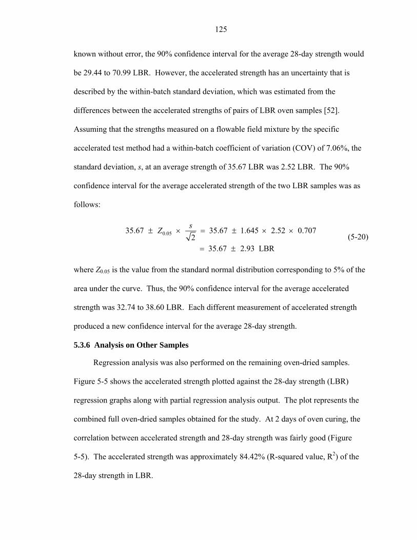
125
known without error, the 90% confidence interval for the average 28-day strength would
be 29.44 to 70.99 LBR. However, the accelerated strength has an uncertainty that is
described by the within-batch standard deviation, which was estimated from the
differences between the accelerated strengths of pairs of LBR oven samples [52].
Assuming that the strengths measured on a flowable field mixture by the specific
accelerated test method had a within-batch coefficient of variation (COV) of 7.06%, the
standard deviation, s, at an average strength of 35.67 LBR was 2.52 LBR. The 90%
confidence interval for the average accelerated strength of the two LBR samples was as
follows:
0.0535.67 35.67 1.645 2.52 0.7072
35.67 2.93 LBR
sZ± × = ± × ×
= ± (5-20)
where Z0.05 is the value from the standard normal distribution corresponding to 5% of the
area under the curve. Thus, the 90% confidence interval for the average accelerated
strength was 32.74 to 38.60 LBR. Each different measurement of accelerated strength
produced a new confidence interval for the average 28-day strength.
5.3.6 Analysis on Other Samples
Regression analysis was also performed on the remaining oven-dried samples.
Figure 5-5 shows the accelerated strength plotted against the 28-day strength (LBR)
regression graphs along with partial regression analysis output. The plot represents the
combined full oven-dried samples obtained for the study. At 2 days of oven curing, the
correlation between accelerated strength and 28-day strength was fairly good (Figure
5-5). The accelerated strength was approximately 84.42% (R-squared value, R2) of the
28-day strength in LBR.

126
y = 3.2039x0.8254
R2 = 0.8442
0.00
50.00
100.00
150.00
200.00
250.00
300.00
350.00
0.00 50.00 100.00 150.00 200.00 250.00 300.00
Accelerated curing strength, LBR
28-d
ay s
tren
gth,
LB
R
Figure 5-5. Accelerated curing vs. 28-day normal curing strength for all mixtures
Further regression analysis was conducted using the 2-day oven dried samples with
56-day normal curing. Figure 5-6 illustrates the accelerated strength plots against the
56-day strength results. Like the 28-day correlation, the 56-day correlation plot showed
promising results. The coefficient of determination (R2-value) was 84.36 %.
y = 3.8565x0.8316
R2 = 0.8436
0.00
50.00
100.00
150.00
200.00
250.00
300.00
350.00
400.00
450.00
0.00 50.00 100.00 150.00 200.00 250.00 300.00
Accelerated curing strength, LBR
56-d
ay s
tren
gth,
LB
R
Figure 5-6. Accelerated curing vs. 56-day normal curing strength for all mixtures
Using the accelerated curing data, a breakdown regression analysis was conducted
on various mixtures with regard to their components and their influence on accelerated

127
curing. The types of mix used were 20% fly ash, 50% slag, and 0% mineral admixture.
Table 5-3 provides a summary of regression equations along with the coefficient of
determinations for accelerated 28- and 56-day LBR strength.
Table 5-3. Summary of regression equations for accelerated (oven) 28-day and 56-day LBR strength
Type of Mix Estimated 28-day Strength Equation, LBR R-square
20% - Fly Ash 0.9122.229y x= 0.876
50% - Slag 0.7603.937y x= 0.863 0% - Mineral Admixture 0.8702.857y x= 0.814
Combined 0.8443.857y x= 0.844
Type of Mix Estimated 56-day Strength Equation, LBR R-square
20% - Fly Ash 0.9053.153y x= 0.907 50% - Slag 0.7974.181y x= 0.842 0% - Mineral Admixture 0.8573.434y x= 0.846
Combined 0.8253.204y x= 0.844
These correlations indicated that 2-day oven dried samples can be used to help
estimate the long-term strength for flowable fill mixtures. It is also clear that the
accelerated strength in LBR provided a meaningful correlation for predicting the 28-day
and 56-day long-term LBR strength. This was evident in their plot. The plots showed
scattered data points with an increasing slope. It should be noted that a power trend line
was used for the two plots. Initially, the regression plots used a linear fitted line, but this
provided poor correlation results. In response to the poor correlation, it was determined
to use power trend to fit the regression plot, which resulted in the better fit.
As the regression equation is used on a project, companion cylinders should be
prepared along with cylinders for accelerated testing. The companion cylinders would be
subjected to standard curing and tested for LBR strength at the designated age. The
measured standard-cured strengths should be compared with the confidence intervals for

128
the estimated strengths based on the companion accelerated strengths. If the measured
strengths constantly fall outside the estimated confidence intervals, the reliability of the
regression line would be questionable. The new companion results should be added to
the data set from the laboratory correlation testing to calculate a new regression line and
its corresponding statistics. This new line should be used for later estimates of potential
later-age strength. The making of companion sets of accelerated and standard-cured
cylinders should be continued until the measured strengths continue to fall within the
corresponding calculated confidence intervals. Once the reliability of the procedure has
been demonstrated, companion cylinders should be made at random intervals to
reconfirm that the procedure continues to be reliable.
5.4 Model Validation and Evaluation of Accuracy
Ensuring the effectiveness of the regression models is an essential part of the
findings and value of this study. In this section, the resultant outcome for the response
variables is evaluated to determine its validity for design purposes. Validation of a fitted
regression equation demonstrates or confirms that the model is sound and effective for
the purpose for which it was intended [40]. The intended purpose of the regression
analysis in this research was to predict or estimate the values of the response variable
precisely enough for engineers to use when designing flowable fill mixtures.
5.4.1 Varying Strength Prediction Models for Trend
An analysis was made involving the regression models for the purpose of
identifying characteristic trends. The following steps were utilized for the analysis:
1. Create a matrix or table.
2. Vary the cement content: 0, 10, 20,…, 200 (@ 10.0 lb/yd3 increments).
3. Vary the w/c ratio: 0.5, 1.5, 2.5,…, 14.5 (@ 1.0 increments).

129
4. Obtain the sand-to-water (s/w) ratio for each mix (see Appendix C).
5. Select mixtures with a ratio that is within 1.73 to 7.20 and label as feasible.
6. Compute estimated strength (LBR and psi) and percent volume change values for feasible mixtures using 28-day and 56-day strength model equations at fixed designed air content and fixed percent of mineral admixtures.
From the matrix table the estimated 28-day and 56-day strengths, along with
percent volume change, were computed for three mixture criteria. The criteria were:
1) 15% fixed air content at 0% mineral admixture, 2) 8% fixed air content at 20% fly ash
mineral admixture, and 3) 10% fixed air content at 50% ground granulated blast-furnace
slag mineral admixture.
Using the estimated strength and volume change values, Figures 5-7 through 5-36
show the relationship of cement content and w/c ratio versus strength and percent volume
change for the three selected mixture criteria mentioned above. Based on the estimated
strength values plotted against cement content and w/c ratio, the plots show increasing
strength for increasing cement content and decreasing strength for increasing w/c ratio.
This translated into the models showing mixtures with high cement contents exhibiting
higher strength and mixtures with high w/c ratio exhibiting low strength. These
identifiable trends demonstrated the predictability for the strength model equations
developed from this study.
Although the strength relationships displayed in the figures identify trends, some
show inaccurate tendencies. Plots are labeled with letters to help designate areas in the
figures with identifiably inaccurate trends. The figures showing strength versus cement
content and w/c ratio contain letters e, f, and g to identify the following:
e = range of test population f = applicable range of prediction equation g = un-applicable range of prediction equation

130
Figure 5-7. Estimated 28-day LBR strength vs. cement content at fixed air (15%) and
fixed 0% mineral admixture
Figure 5-8. Estimated 56-day LBR strength vs. cement content at fixed air (15%) and
fixed 0% mineral admixture
0.00
20.00
40.00
60.00
80.00
100.00
120.00
140.00
160.00
180.00
200.00
0 50 100 150 200 250
Cement content, lbs/yd3
Stre
ngth
, LB
R
e
f
e
g
0.00
50.00
100.00
150.00
200.00
250.00
0 50 100 150 200 250
Cement content, lbs/yd3
Stre
ngth
, LB
R
f
e
g

131
Figure 5-9. Estimated 28-day compressive strength vs. cement content at fixed air (15%)
and fixed 0% mineral admixture
Figure 5-10. Estimated 28-day compressive strength vs. cement content at fixed air
(15%) and fixed 0% mineral admixture
0.00
20.00
40.00
60.00
80.00
100.00
120.00
140.00
160.00
0 50 100 150 200 250
Cement content, lbs/yd3
Stre
ngth
, psi
e,f
0.00
20.00
40.00
60.00
80.00
100.00
120.00
140.00
160.00
180.00
0 50 100 150 200 250
Cement content, lbs/yd3
Stre
ngth
, psi
f g
e

132
0.00
0.50
1.00
1.50
2.00
2.50
3.00
3.50
4.00
0 50 100 150 200 250
Cement content, lbs/yd3
Volu
me
chan
ge, %
Minimum Mean Maximum
Figure 5-11. Estimated volume change vs. cement content at fixed air (15%) and fixed
0% mineral admixture
Figure 5-12. Estimated 28-day LBR strength vs. w/c ratio at fixed air (15%) and fixed
0% mineral admixture
0.00
20.00
40.00
60.00
80.00
100.00
120.00
140.00
160.00
180.00
0 2 4 6 8 10 12 14 16
w/c ratio
Stre
ngth
, LB
R
e, f g

133
Figure 5-13. Estimated 56-day LBR strength vs. w/c ratio at fixed air (15%) and fixed
0% mineral admixture
Figure 5-14. Estimated 28-day compressive strength vs. w/c ratio at fixed air (15%) and
fixed 0% mineral admixture
0.00
50.00
100.00
150.00
200.00
250.00
0 2 4 6 8 10 12 14 16
w/c ratio
Stre
ngth
, psi
g e, f
0.00
50.00
100.00
150.00
200.00
250.00
300.00
0 2 4 6 8 10 12 14 16
w/c ratio
Stre
ngth
, LB
Re, f g

134
Figure 5-15. Estimated 56-day compressive strength vs. w/c ratio at fixed air (15%) and
fixed 0% mineral admixture
0.00
1.00
2.00
3.00
4.00
5.00
6.00
0 2 4 6 8 10 12 14 16
w/c ratio
Volu
me
chan
ge, %
Minimum Mean Maximum
Figure 5-16. Estimated volume change vs. w/c ratio at fixed air (15%) and fixed 0%
mineral admixture
0.00
20.00
40.00
60.00
80.00
100.00
120.00
140.00
160.00
0 50 100 150 200 250
Cement content, lbs/yd3
Stre
ngth
, psi
e, f

135
Figure 5-17. Estimated 28-day LBR strength vs. cement content at fixed air (8%) and
fixed 20% fly ash mineral admixture
Figure 5-18. Estimated 56-day LBR strength vs. cement content at fixed air (8%) and
fixed 20% fly ash mineral admixture
0.00
20.00
40.00
60.00
80.00
100.00
120.00
140.00
160.00
180.00
200.00
0 50 100 150 200 250
Cement content, lbs/yd3
Stre
ngth
, LB
R
g f
e
0.00
50.00
100.00
150.00
200.00
250.00
0 50 100 150 200 250
Cement content, lbs/yd3
Stre
ngth
, LB
R
e,f g

136
Figure 5-19. Estimated 28-day compressive strength vs. cement content at fixed air (8%)
and fixed 20% fly ash mineral admixture
Figure 5-20. Estimated 56-day compressive strength vs. cement content at fixed air (8%)
and fixed 20% fly ash mineral admixture
0.00
20.00
40.00
60.00
80.00
100.00
120.00
0 50 100 150 200 250
Cement content, lbs/yd3
Stre
ngth
, psi
f g
e
0.00
20.00
40.00
60.00
80.00
100.00
120.00
140.00
0 50 100 150 200 250
Cement content, lbs/yd3
Stre
ngth
, psi
e,f

137
0.00
0.50
1.00
1.50
2.00
2.50
0 50 100 150 200 250
Cement content, lbs/yd3
Volu
me
chan
ge, %
Minimum Mean Maximum
Figure 5-21. Estimated volume change vs. cement content at fixed air (8%) and fixed
20% fly ash mineral admixture
Figure 5-22. Estimated 28-day LBR strength vs. w/c ratio at fixed air (8%) and fixed
20% fly ash mineral admixture
0.00
50.00
100.00
150.00
200.00
250.00
0 2 4 6 8 10 12 14 16
w/c ratio
Stre
ngth
, LB
R
g e,f

138
Figure 5-23. Estimated 56-day LBR strength vs. w/c ratio at fixed air (8%) and fixed
20% fly ash mineral admixture
Figure 5-24. Estimated 28-day compressive strength vs. w/c ratio at fixed air (8%) and
fixed 20% fly ash mineral admixture
0.00
20.00
40.00
60.00
80.00
100.00
120.00
140.00
160.00
180.00
0 2 4 6 8 10 12 14 16
w/c ratio
Stre
ngth
, psi
g e,f
0.00
50.00
100.00
150.00
200.00
250.00
0 2 4 6 8 10 12 14 16
w/c ratio
Stre
ngth
, LB
Rg e,f

139
Figure 5-25. Estimated 56-day compressive strength vs. w/c ratio at fixed air (8%) and
fixed 20% fly ash mineral admixture
0.00
0.50
1.00
1.50
2.00
2.50
3.00
0 2 4 6 8 10 12 14 16
w/c ratio
Volu
me
chan
ge, %
Minimum Mean Maximum
Figure 5-26. Estimated volume change vs. w/c ratio at fixed air (8%) and fixed 20% fly
ash mineral admixture
0.00
20.00
40.00
60.00
80.00
100.00
120.00
0 2 4 6 8 10 12 14 16
w/c ratio
Stre
ngth
, psi
g e,f

140
Figure 5-27. Estimated 28-day LBR strength vs. cement content at fixed air (10%) and
fixed 50% ground granulated blast-furnace slag mineral admixture
Figure 5-28. Estimated 56-day LBR strength vs. cement content at fixed air (10%) and
fixed 50% ground granulated blast-furnace slag mineral admixture
0.00
50.00
100.00
150.00
200.00
250.00
0 50 100 150 200 250
Cement content, lbs/yd3
Stre
ngth
, LB
Rg f
e
0.00
50.00
100.00
150.00
200.00
250.00
300.00
0 50 100 150 200 250
Cement content, lbs/yd3
Stre
ngth
, LB
R
g e,f

141
Figure 5-29. Estimated 28-day compressive strength vs. cement content at fixed air
(10%) and fixed 50% ground granulated blast-furnace slag mineral admixture
Figure 5-30. Estimated 56-day compressive strength vs. cement content at fixed air
(10%) and fixed 50% ground granulated blast-furnace slag mineral admixture
0.00
20.00
40.00
60.00
80.00
100.00
120.00
140.00
160.00
0 50 100 150 200 250
Cement content, lbs/yd3
Stre
ngth
, psi
e,f
0.00
20.00
40.00
60.00
80.00
100.00
120.00
140.00
160.00
0 50 100 150 200 250
Cement content, lbs/yd3
Stre
ngth
, psi
g f
e

142
0.00
0.20
0.40
0.60
0.80
1.00
1.20
1.40
1.60
1.80
0 50 100 150 200 250
Cement content, lbs/yd3
Volu
me
chan
ge, %
Minimum Mean Maximum
Figure 5-31. Estimated volume change vs. cement content at fixed air (10%) and fixed
50% ground granulated blast-furnace slag mineral admixture
Figure 5-32. Estimated 28-day LBR strength vs. w/c ratio at fixed air (10%) and fixed
50% ground granulated blast-furnace slag mineral admixture
0.00
50.00
100.00
150.00
200.00
250.00
0 2 4 6 8 10 12 14 16
w/c ratio
Stre
ngth
, LB
R
g e,f

143
Figure 5-33. Estimated 56-day LBR strength vs. w/c ratio at fixed air (10%) and fixed
50% ground granulated blast-furnace slag mineral admixture
Figure 5-34. Estimated 28-day compressive strength vs. w/c ratio at fixed air (10%) and
fixed 50% ground granulated blast-furnace slag mineral admixture
0.00
50.00
100.00
150.00
200.00
250.00
300.00
0 2 4 6 8 10 12 14 16
w/c ratio
Stre
ngth
, LB
R
g e,f
0.00
20.00
40.00
60.00
80.00
100.00
120.00
140.00
160.00
180.00
0 2 4 6 8 10 12 14 16
w/c ratio
Stre
ngth
, psi
g e,f

144
Figure 5-35. Estimated 56-day compressive strength vs. w/c ratio at fixed air (10%) and
fixed 50% ground granulated blast-furnace slag mineral admixture
0.00
0.20
0.40
0.60
0.80
1.00
1.20
1.40
1.60
1.80
2.00
0 2 4 6 8 10 12 14 16
w/c ratio
Volu
me
chan
ge, %
Minimum Mean Maximum
Figure 5-36. Estimated volume change vs. w/c ratio at fixed air (10%) and fixed 50%
ground granulated blast-furnace slag mineral admixture
0.00
50.00
100.00
150.00
200.00
250.00
300.00
0 2 4 6 8 10 12 14 16
w/c ratio
Stre
ngth
, psi
g e,f

145
The letters e, f, and g were inserted into the charts in order to provide a visual
context for areas where the prediction equations grossly estimate and underestimate the
strength. For example, Figure 5-12 shows the estimated 28-day LBR strength versus w/c
ratio at fixed 15% air content and fixed 0% mineral admixture. The plot area labeled g
specifies the region where the prediction equation overestimates the strength. The plots
help to illustrate and define areas to avoid when using the prediction models.
Plots which display percent volume change versus w/c ratio and cement content do
not contain any letters, instead, these figures contain lines to indicate the minimum, mean
and maximum of the overall estimated percent volume change. This approach allows for
one to better examine the estimated values from a low- and high-end perspective due to
the lack of identifiable trends in volume change plots.
5.4.2 Comparison of Strength Prediction Models
A comparison was made between the strength prediction models developed from
the NCHRP studies on flowable fill and the regression models formed from this
dissertation research. Table 5-4 summarizes the NCHRP’s mixture proportions used in
their study. In comparing the two models, it was important to identify mixtures that were
similar in design. The design in this case meant mixtures that included concrete sand
(silica sand) as fines aggregates and 0% mineral admixtures (no fly ash), and into which
air-entrainment was introduced during batching. In Chapter 2, it was specified that the
NCHRP study formed two models for estimating the compressive strength of flowable
fill, and those were air-entrained and nonair-entrained models. For this comparison, the
NCHRP’s air-entrained model was utilized. This made for a fair comparison between
models due to the fact that the flowable fill mixtures used to design the models for this
research study were all entirely air-entrained mixes. The following NCHRP mixtures

146
Table 5-4. NCHRP’s CLSM mixture proportions and fresh properties [38] Cement Content Mixture
No.a (kg/m3) (lbs/yd3) Fly Ash Type
Fly Ash Content(kg/m3)
Fine Aggregate Type
Water Demand (kg/m3)
Flow (cm)
Total Bleeding(%)
Air Content(%)
Fresh Unit Weight (kg/m3)
W/C Ratio
1 30 51 Class C 180 Concrete sand 211 20 NA 0.9 1965 7.0 2 60 101 Class C 180 Concrete sand 206 20 2.45 1 2108 3.4 1R 30 51 Class C 180 Concrete sand 206 12 2.08 0.9 1974 6.9 15 30 51 Class C 360 Foundry sand 486 20 0.13 2.8 1741 16.2 3 60 101 Class C 360 Bottom ash 577 17.8 4.32 1.7 1754 9.6 8 60 101 High carbon 180 Foundry sand 532 24.1 1.04 3.3 1647 8.9 10 30 51 High carbon 180 Bottom ash 628 14 4.81 2 1681 20.9 9 60 101 Class F 360 Foundry sand 520 20 0.54 2.5 1684 8.7 5 60 101 Class F 180 Bottom ash 600 17.8 5.84 2.5 1739 10.0 12 30 51 Class C 360 Bottom ash 572 21.6 3.64 2.7 1774 19.1 4 30 51 Class F 360 Concrete sand 220 20 0.39 2.2 2199 7.3 7 30 51 Class F 180 Foundry sand 501 20 0.57 2.1 1817 16.7 3R 60 101 Class C 360 Bottom ash 541 20 2.58 2.1 1997 9.0 4R 30 51 Class F 360 Concrete sand 220 21.6 2.92 1.8 2211 7.3 24 60 101 Class F 1200 None 486 24 2.25 2.8 1635 8.1 23 60 101 None 0 Bottom ash 454 14 1.3 28.5 1382 7.6 18 60 101 None 0 Concrete sand 200 21.6 0.7 16.5 1826 3.3 14 60 101 Class F 360 Concrete sand 216 21.6 1 1.3 2174 3.6 2R 60 101 Class C 180 Concrete sand 206 25 0.21 0.5 2291 3.4 29 60 101 Foundry sand 0 None 373 23 0.28 2.6 1812 6.2 30 30 51 Foundry sand 0 None 414 20 0.4 2 1789 13.8 17* 30 51 None 0 Bottom ash 582 12.7 4.35 20 1447 19.4 11 60 101 High carbon 360 Bottom ash 573 23 6.42 1.7 1743 9.6 6 30 51 High carbon 360 Concrete sand 315 20 2.26 1.3 2103 10.5 16 30 51 None 0 Concrete sand 295 20 2.33 16 1922 9.8 21 30 51 None 0 Concrete sand 170 18 0.62 25.5 1789 5.7 22 60 101 None 0 Concrete sand 131 20 0.05 26.5 1748 2.2 22R 60 101 None 0 Concrete sand 136 18 0.43 25.5 1802 2.3 5R 60 101 Class F 180 Bottom ash 600 16 7.2 1.4 1887 10.0 26* 60 101 None 0 Concrete sand 136 16.5 0 25.5 1802 2.3 16R 30 51 None 0 Concrete sand 295 19.1 2.35 15.5 1874 9.8 13 60 101 Class C 360 Foundry sand 499 20 0 1.8 1902 8.3 25 60 101 High carbon 1200 None 853 24 7.38 1.3 1322 14.2 19* 30 51 None 0 Bottom ash 492 13 1.08 25 1385 16.4 20* 60 101 None 0 Bottom ash 525 13 3.41 18.5 1485 8.8 27 60 101 Class C 1200 None 486 23 1.28 0.7 1638 8.1 20R 60 101 None 0 Bottom ash 525 13 1.44 15.5 1511 8.8 28 30 51 Class F 180 Concrete sand 220 20 1.33 1.4 2182 7.3 Note: aR = mixtures that were replicated for statistical purposes; * = mixtures batched for a third time due to malfunctions during batching or testing

147
used to compare the models were: 16, 21, 22, 22r, 26*, and 16r. Using NCHRP’s model
(Equation 2-7) and the 28-day compressive strength model formulated in this dissertation,
the required values for the variables were entered and the estimated compressive strength
from both models, shown in Table 5-5, were plotted in Figure 5-37 and correlated with
Table 5-5. Comparison of the NCHRP measured and predicted 28-day strength for air-entrained mixtures strength prediction model
Confidence, 95% Mixture No.
Measured Strength (psi)
NCHRP Strength (psi)
Dissertation Strength (psi)
Lower (psi)
Upper (psi)
16 18.85 16.49 26.83 13.84 39.83 21 23.20 45.45 18.67 5.93 31.41 22 105.85 106.09 97.82 84.83 110.81 22ra 139.20 103.96 94.60 81.60 107.59 26b 165.30 103.96 94.60 81.60 107.59 16ra 21.75 16.49 26.28 13.29 39.27 Note: amixtures that were replicated for statistical purposes; and bmixture batched for a third time due to malfunctions during batching or testing
R2Dissertation = 0.90
R2NCHRP = 0.86
0
20
40
60
80
100
120
140
0.00 20.00 40.00 60.00 80.00 100.00 120.00 140.00 160.00 180.00
Measured Strength, psi
Pred
icte
d St
reng
th, p
si
NCHRP Dissertation Linear (Dissertation ) Linear (NCHRP)
Figure 5-37. Comparison of measured and predicted 28-days strength

148
the measured compressive strength for the six flowable fill mixtures. Both models
yielded very good correlation in predicting 28-day compressive strength. The models
from the NCHRP and this research study yielded, respectively, R2 values of 0.86 and
0.90.
A second effort was undertaken to compare the formulated dissertation regression
models with other published flowable fill strength prediction models. The two strength
prediction models used are Equation 2-6 by Bhat and Equation 2-7 by NCHRP. The
approach utilized to compare the models entails varying the w/c ratio (c), holding the
cement content (a), air content (b) and mineral admixture (d) fixed. The fixed values
used for cement content, air content and mineral admixtures were, respectively, 100
lb/yd3, 15% and 0%. This provided an estimated 28-day compressive strength for all
three prediction equations. Table 5-6 shows a comparison of estimated 28-day compres-
sive strength for the three prediction models.
Figures 5-38 and 5-39 provide a more illustrative comparison of the estimated
compressive strength from the models. From the table and figures, the formula
developed by Bhat estimate the 28-day compressive strength much higher than the other
two models; whereas, the dissertation and NCHRP models estimate the 28-day compres-
sive strength at lower approximations. When comparing the strength estimation of the
dissertation to the NCHRP’s, the predictive formula of the dissertation estimates the
compressive strength slightly lower than the NCHRP formula. Based on this informa-
tion, one can conclude that a slight improvement exists with using the dissertation model
for estimating the 28-day compressive strength.

149
Table 5-6. Comparison of estimated 28-day compressive strength
Bhat Model NCHRP Model Dissertation Model W/C Ratio Strength
(MPa) Strength (psi)
Strength (MPa)
Strength (psi)
Strength (MPa)
Strength (psi)
2.0 16.24 2355 0.76 111 0.76 110 2.2 12.29 1783 0.73 106 0.71 103 2.4 9.55 1386 0.69 101 0.66 96 2.6 7.59 1101 0.66 96 0.62 90 2.8 6.16 893 0.63 91 0.58 84 3.0 5.07 736 0.60 87 0.54 78 3.2 4.25 616 0.57 83 0.50 72 3.4 3.60 523 0.54 79 0.46 67 3.6 3.09 449 0.52 75 0.43 62 3.8 2.69 390 0.49 72 0.40 58 4.0 2.36 342 0.47 68 0.37 53 4.2 2.09 303 0.45 65 0.34 49 4.4 1.86 270 0.43 62 0.31 45 4.6 1.68 243 0.41 59 0.28 41 4.8 1.52 221 0.39 56 0.26 38 5.0 1.39 201 0.37 53 0.24 35 5.2 1.28 185 0.35 51 0.22 32 5.4 1.18 171 0.33 48 0.20 29 5.6 1.10 159 0.32 46 0.19 27 5.8 1.02 149 0.30 44 0.17 25 6.0 0.96 139 0.29 42 0.16 23 6.2 0.91 131 0.28 40 0.15 22 6.4 0.86 124 0.26 38 0.14 21 6.6 0.82 118 0.25 36 0.14 20 6.8 0.78 113 0.24 34 0.13 19 7.0 0.74 108 0.23 33 0.13 19 7.2 0.71 104 0.22 31 0.13 19 7.4 0.69 100 0.21 30 0.13 19 7.6 0.66 96 0.20 28 0.13 19 7.8 0.64 93 0.19 27 0.14 20 8.0 0.62 90 0.18 26 0.14 21

150
0
500
1000
1500
2000
2500
0 1 2 3 4 5 6 7 8 9w/c ratio
Stre
ngth
, psi
NCHRP's Model Dissertation's Model Bhat's Model
Figure 5-38. Comparison of estimated 28-day compressive strength for Bhat, NCHRP, and dissertation models
0
20
40
60
80
100
120
0 1 2 3 4 5 6 7 8 9w/c ratio
Stre
ngth
, psi
NCHRP's Model Dissertation's Model
Figure 5-39. Comparison of estimated 28-day compressive strength for NCHRP and dissertation models
5.4.3 Mixture Design Examples to Validate Models
In this section, the design of 11 validation flowable fill mixtures is discussed. After
designing and batching the mixtures in the laboratory, the exact air content was used
along with other design parameters to estimate the LBR strength, compressive strength
and percent volume change for each mixture. The validation flowable fill mixtures were

151
designed using the volumetric method discussed in Chapter 3. The following outlines the
two steps used for designing 1-yd3 mixtures.
• Step 1: Determine the amount of materials required for mixtures with the following design criteria:
a. Mix #1v i. cementitious content = 195 lb/yd3 ii. w/c = 2.25 iii. air content = 8.5 ± 2.5% iv. mineral admixtures = 50% slag
b. Mix #2v i. cementitious content = 69 lb/yd3 ii. w/c = 6.0 iii. air content = 15.5 ± 2.5% iv. mineral admixtures = 20% fly ash
c. Mix #3v i. cementitious content = 165 lb/yd3 ii. w/c = 3.0 iii. air content = 10.0 ± 2.5% iv. mineral admixtures = 0%
The following are known properties for the materials that will be used to
create the mixtures:
Sc = 3.15 specific gravity of cement Ss = 2.42 specific gravity of slag Sf = 2.36 specific gravity of fly ash Sag = 2.63 specific gravity of fine aggregate N = 3.00 percent of natural moisture content for fine aggregate L = 0.40 percent absorption for fine aggregate
Solution for Mix #1v 1. Calculate weight of cement, lb/yd3.
cementitious content
195 0.50 97.50w pC S= ×
= × =

152
2. Calculate weight of slag, lb/yd3.
cementitious content195 97.50 97.50
w wS C= −= − =
3. Calculate weight of water, lb/yd3.
( )
( )w / c ratio
2.25 97.50 97.50 438.75w w wW C S= × +
= × + =
4. Calculate absolute volume of cement, ft3/yd3.
397.50 0.496 ft62.4 3.15 62.4
wv
c
CCS
= = =× ×
5. Calculate absolute volume of slag, ft3/yd3.
397.50 0.646 ft62.4 2.42 62.4
wv
s
SSS
= = =× ×
6. Calculate absolute volume of water, ft3/yd3.
3438.75 7.031 ft62.4 62.4
wv
WW = = =
7. Calculate absolute volume of target air content, ft3/yd3.
327 8.5 27 2.295 ft100 100
pv
AA
× ×= = =
8. Calculate total absolute volume of known ingredients
310.468 ftv v v vC S W A+ + + =
9. Calculate absolute volume of saturated-surface-dry (SSD) fine aggregates, ft3/yd3.
327 ( ) 16.532 ftvs v v v vFA C S W A= − + + + =
10. Calculate weight of saturated-surface-dry fine aggregates, lb/yd3.
62.4
16.532 2.63 62.4 2713.10ws vs agFA FA S= × ×
= × × =

153
11. Calculate the sand-to-water (s/w) ratio (s/w ratio range 1.73 – 7.20).
2713.10 6.184438.75
ws
w
FASW W
= =
12. Calculate weight of fine aggregate based on natural moisture content, lb/yd3.
11
1 0.032713.10 2783.361 0.004
wn wsNFA FAL
+= ×
++
= × =+
13. Correct the weight of water content due to percentage of moisture difference, lb/yd3.
2783.36 2713.10 70.26
438.75 70.26 509.01
ws wn
w
W FA FAW W WW
Δ = − = − == + Δ= + =
Table 5-7 provides a summary of materials required for the eleven validation
mixtures. The bold face values are the weight amounts for the cement, slag, fly
ash, sand, and water needed for batching each mix. The sand-to-water ratio shown
for the three mixtures fall within the recommended specified feasible mixture sand-
to-water ratio range of 1.73 to 7.20.
After obtaining the batching information and ensuring the mixtures met the
sand-to-water ratio criteria for the three mixtures, the three validation mixtures
were batched. Table 5-8 shows the plastic properties for the batched validation
mixtures. In accordance to their design, all mixes achieved (exact) air within their
respective designed target air content.
• Step 2: Determine the 28-day strength and the percent volume change using the mixture parameters.
Solution: The 28-day and 56-day strengths of flowable fill and the percent volume
change can be estimated by using Equations 5-3 through 5-7. When estimating the

154
Table 5-7. Summary of materials required for validation mixtures Per 1.0 cu. yd. Batch
Mix No.a
Cement Content (lb/yd3)
W/C Ratio
Mineral Admix- tures (%)
Target Air Content (±2.5%)
Cw (lbs)
Sw (lbs)
Fw (lbs)
Ww (lbs)
Cv
Sv
Fv
Wv
Av
FAvs
FAws (lbs)
S/W
FAwn
ΔW
W
1v 195 2.25 50 8.50 97.50 97.50 0.00 438.75 0.50 0.65 0.00 7.03 2.30 16.53 2713.11 6.18 2783.37 70.26 509.01 2v 69 6.00 20 15.50 55.20 0.00 13.80 414.00 0.28 0.00 0.09 6.63 4.19 15.81 2594.31 6.27 2661.49 67.18 481.18 3v 165 3.00 0 10.00 165.00 0.00 0.00 495.00 0.84 0.00 0.00 7.93 2.70 15.53 2548.31 5.15 2614.30 65.99 560.99 4v 60 7.50 50 10.50 30.00 30.00 0.00 450.00 0.15 0.20 0.00 7.21 2.84 16.60 2724.62 6.05 2795.17 70.56 520.56 5v 90 5.50 50 10.50 45.00 45.00 0.00 495.00 0.23 0.30 0.00 7.93 2.84 15.71 2577.44 5.21 2644.19 66.75 561.75 6v 70 9.50 20 6.00 56.00 0.00 14.00 665.00 0.28 0.00 0.09 10.66 1.62 14.35 2354.24 3.54 2415.21 60.97 725.97 7v 80 6.50 20 6.00 64.00 0.00 16.00 520.00 0.33 0.00 0.11 8.33 1.62 16.62 2726.74 5.24 2797.35 70.61 590.61 8v 110 4.50 20 6.00 88.00 0.00 22.00 495.00 0.45 0.00 0.15 7.93 1.62 16.85 2765.93 5.59 2837.56 71.63 566.63 9v 60 7.50 0 15.00 60.00 0.00 0.00 450.00 0.31 0.00 0.00 7.21 4.05 15.43 2532.78 5.63 2598.36 65.59 515.5910v 100 4.50 0 15.00 100.00 0.00 0.00 450.00 0.51 0.00 0.00 7.21 4.05 15.23 2499.38 5.55 2564.10 64.72 514.7211v 130 3.50 0 15.00 130.00 0.00 0.00 455.00 0.66 0.00 0.00 7.29 4.05 15.00 2461.18 5.41 2524.92 63.74 518.74
Per 5.5 cu. ft. Batch Mix No. a
Cement Content (lb/yd3)
W/C Ratio
Mineral Admix- tures (%)
Target Air Content (±2.5%)
Cw (lbs)
Sw (lbs)
Fw (lbs)
Ww (lbs) Cv Sv Fv Wv Av FAvs
FAws (lbs) S/W FAwn ΔW W
1v 195 2.25 50 8.50 19.86 19.86 0.00 89.38 0.10 0.13 0.00 1.43 0.47 3.37 552.67 1.26 566.98 14.31 103.69 2v 69 6.00 20 15.50 11.24 0.00 2.81 84.33 0.06 0.00 0.02 1.35 0.85 3.22 528.47 1.28 542.16 13.69 98.02 3v 165 3.00 0 10.00 33.61 0.00 0.00 100.83 0.17 0.00 0.00 1.62 0.55 3.16 519.10 1.05 532.54 13.44 114.28 4v 60 7.50 50 10.50 6.11 6.11 0.00 91.67 0.03 0.04 0.00 1.47 0.58 3.38 555.01 1.23 569.39 14.37 106.04 5v 90 5.50 50 10.50 9.17 9.17 0.00 100.83 0.05 0.06 0.00 1.62 0.58 3.20 525.03 1.06 538.63 13.60 114.43 6v 70 9.50 20 6.00 11.41 0.00 2.85 135.46 0.06 0.00 0.02 2.17 0.33 2.92 479.57 0.72 491.99 12.42 147.88 7v 80 6.50 20 6.00 13.04 0.00 3.26 105.93 0.07 0.00 0.02 1.70 0.33 3.38 555.45 1.07 569.83 14.38 120.31 8v 110 4.50 20 6.00 17.93 0.00 4.48 100.83 0.09 0.00 0.03 1.62 0.33 3.43 563.43 1.14 578.02 14.59 115.42 9v 60 7.50 0 15.00 12.22 0.00 0.00 91.67 0.06 0.00 0.00 1.47 0.83 3.14 515.94 1.15 529.30 13.36 105.0310v 100 4.50 0 15.00 20.37 0.00 0.00 91.67 0.10 0.00 0.00 1.47 0.83 3.10 509.13 1.13 522.32 13.18 104.8511v 130 3.50 0 15.00 26.48 0.00 0.00 92.69 0.13 0.00 0.00 1.49 0.83 3.05 501.35 1.10 514.33 12.98 105.67Note:
a v = denotes validation mix

155
Table 5-8. Summary of plastic properties of validation mixture models Air Content Batch Mix
No. AEA (ml)
Flow (in.) Target
(%) Achieved (%)
Unit Weight (lb/t3)
Mixture Temperature (°F)
1v 25 5.50 8.5 ± 2.5 11.00 113.04 75.00 1vr 40 5.50 8.5 ± 2.5 10.50 113.92 77.00 2v 40 0.00 15.5 ± 2.5 16.00 106.40 75.00 2vr 40 0.00 15.5 ± 2.5 14.00 109.28 77.00 3v 45 8.00 10.5 ± 2.5 7.60 119.36 80.00 3vr 45 8.00 10.5 ± 2.5 7.70 117.36 80.00 4v 50 5.50 10.5 ± 2.5 9.50 101.04 74.00 5v 25 4.50 10.5 ± 2.5 11.00 113.16 74.00 6v 25 0.00 6.0 ± 2.5 5.00 124.24 72.00 7v 30 0.00 6.0 ± 2.5 9.75 116.88 74.00 8v 30 4.50 6.0 ± 2.5 8.50 119.04 74.00 9v 40 5.50 15.0 ± 2.5 14.70 106.56 72.00 10v 40 5.50 15.0 ± 2.5 14.70 107.92 75.00 11v 50 5.50 15.0 ± 2.5 12.75 110.96 75.00 Note: r = denotes repeat
responses, the designed air or achieved (exact) air content for the mixture can be
used. It is recommended to use the achieved air content as opposed to the designed
air content. The designed air can be used for preliminary design, so as to get an
approximate estimated strength for a particular flowable fill mixture prior to
batching.
228 day LBR
2 2
ˆ 299.040 0.928 18.780 24.817 3.214 0.000756
1.187 0.0792 0.0337 0.145 0.004261.150 0.0304 0.114
y a b c d a
c d ab ac adbc bd cd
− = + − − − −
+ + + − −+ + −
56 day LBR
2 2 2
ˆ 917.423 4.029 33.638 129.930 1.767
0.00840 4.964 0.0601 0.0919 0.3590.00373 2.602 0.0375 0.186
y a b c d
a c d ab acad bc bd cd
− = − − − −
+ + + + +− + + −
228 day psi
2 2
ˆ 94.934 1.523 0.681 45.616 1.230 0.00294
3.365 0.0272 0.00964 0.0635 0.01000.232 0.0418 0.145
y a b c d a
c d ab ac adbc bd cd
− = + − − + −
+ + − − −+ − −

156
256 day psi
2 2
ˆ 152.831 0.244 14.130 1.507 1.415 0.00135
1.215 0.0289 0.0527 0.0130 0.0005651.144 0.00419 0.0103
y a b c d a
c d ab ac adbc bd cd
− = − − − − +
− + + + −+ − +
% volume change
2 2 2
ˆ 3.945 0.00457 0.193 0.667 0.0284
0.0000105 0.0373 0.000185 0.0001160.00904 0.0000700 0.0128 0.0001650.00445
y a b c d
a c d abac ad bc bdcd
= − − + − +
+ + − −+ − + −−
For Mix #1v:
28 day LBR
2 2 2
ˆ 299.040 0.928(195) 18.780(8.5) 24.817 (2.25)
3.214(50) 0.000756(195) 1.187 (2.25) 0.0792(50).0337 (195 8.5) 0.145(195 2.25) 0.00426(195 50)1.150(8.5 2.25) 0.0304(8.5 50) 0.114(2.25 50)
y − = + − −
− − + ++ × − × − ×+ × + × − ×
28 day LBRˆ 251.978 LBRy − =
( ) ( ) ( )( ) ( ) ( ) ( )
( ) ( ) ( )( ) ( ) ( )
56 day LBR
2 2 2
ˆ 917.423 4.029 195 33.638 8.5 129.930 2.25
1.767 50 0.00840 195 4.964 2.25 0.0601 50
0.0919 195 8.5 0.359 195 2.25 0.00373 195 50
2.602 8.5 2.25 0.0375 8.5 50 0.186 2.25 50
y − = − − −
− + + +
+ × + × − ×
+ × + × − ×
56 day LBRˆ 278.348y LBR− =
28 day psi
2 2 2
ˆ 94.934 1.523 (195) 0.681(8.5) 45.616(2.25) 1.230(50)
0.00294 (195) 3.365 (2.25) 0.0272 (50)0.00964 (195 8.5) 0.0635 (195 2.25) 0.0100 (195 50)0.232 (8.5 2.25) 0.0418 (8.5 50) 0.145 (2.25 50)
y − = + − − +
− + +− × − × − ×+ × − × − ×
28 day psiˆ 147.135 psiy − =
( ) ( ) ( ) ( )( ) ( ) ( ) ( )
( ) ( ) ( )( ) ( )
56 day psi
2 2 2
ˆ 152.831 0.244 195 14.130 8.5 1.507 2.25 1.415 50
0.00135 195 1.215 2.25 0.0289 50 0.0527 195 8.5
0.0130 195 2.25 0.000565 195 50 1.144 8.5 2.25
0.00419 8.5 50 0.0103 2.25 50
y − = − − − −
+ − + + ×
+ × − × + ×
− × + ×
56 day psiˆ 137.411y psi− =

157
% volume change
2 2
2
ˆ 3.945 0.00457 (195) 0.193(8.5) 0.667 (2.25)
0.000185(50) 0.0284(50) 0.0000105(195)
0.0373(2.25) 0.000116(195 8.5) 0.00904(195 2.25)0.0000700(195 50) 0.0128(8.5 2.25)0.000165(8.5 50
y = − − + −
− + +
+ − × + ×− × + ×− × ) 0.00445(2.25 50)− ×
% volume changeˆ 0.3835%y = −
Tables 5-9 and 5-10 show summaries of estimated 28-day and 56-day
strength and percent volume change for the validation mixes 1v through 6v and 7v
through 11v, respectively. The tables also show a comparison between the
experimental results and the estimated (calculated) results.
The results of the predicted (estimated) and measured strengths for validating
the mixtures of the model are plotted and correlated in Figures 5-40 through 5-42.
The R2 values for the 28-day LBR strength, 28-day compressive strength, and
28-day oven strength results, respectively, are 0.864, 0.916, and 0.868.
5.5 Summary of Model Equations and Limitations
Table 5-11 summarized the recommended predictive formulas developed in this
study. The table also lists the variables along with their applicable ranges. To help
determine the suitable range for cement content (a), air content (b) and w/c ratio (c), a
succession of plots were generated by varying the variables and estimating LBR and
compressive strength. The estimated strength was plotted and analyzed, the applicable
range was later selected after extensive evaluation. Appendix D shows plots of estimated
28- and 56-day strength using applicable ranges of prediction equation variables.

158
Table 5-9. Comparison of estimated and experimental results for
batch mixes 1v through 6v 95% Confidence Results Batch
Mix No.
Testing Interval Lower Upper Estimated Experimentala
Estimated Strength (Oven)b
28-day strength, LBR 226 278 252 216 220 28-day strength, psi 134 160 147 101 -- 56-day strength, LBR 249 307 278 223 273 56-day strength, psi 121 153 137 100 --
1v
24-hr volume change, % -0.93 0.16 2.52 NR -- 28-day strength, LBR -23 28 3 25 35 28-day strength, psi -14 12 -1 13 -- 56-day strength, LBR -10 48 19 29 43 56-day strength, psi 5 37 21 16 --
2v
24-hr volume change, % 0.20 1.29 0.75 NR -- 28-day strength, LBR 173 224 198 180 269 28-day strength, psi 99 125 112 99 -- 56-day strength, LBR 204 262 233 238 335 56-day strength, psi 109 141 125 138 --
3v
24-hr volume change, % -0.02 1.07 0.52 NR -- 28-day strength, LBR 61 112 86 13 18 28-day strength, psi 24 11 37 17 -- 56-day strength, LBR 60 119 89 12 22 56-day strength, psi 32 64 48 15 --
4v
24-hr volume change, % -1.88 -0.79 -1.34 NR -- 28-day strength, LBR 78 130 104 55 81 28-day strength, psi 33 59 46 32 -- 56-day strength, LBR 100 158 129 NR 100 56-day strength, psi 53 85 69 NR --
5v
24-hr volume change, % -0.77 0.32 -0.22 0.65 -- 28-day strength, LBR 25 76 51 51 93 28-day strength, psi -4 22 9 20 -- 56-day strength, LBR 39 98 69 75 115 56-day strength, psi -3 29 13 31 --
6v
24-hr volume change, % -0.65 0.44 -0.11 NR -- aNR = Not recorded b-- = No data

159
Table 5-10. Comparison of estimated and experimental results for batch mixes 7v through 11v
95% Confidence Results Batch Mix No.
Testing Interval Lower Upper Estimated Experimentala
Estimated Strength (Oven)b
28-day strength, LBR 21 75 50 13 49 28-day strength, psi -9 17 4 13 -- 56-day strength, LBR 46 104 75 NR 60 56-day strength, psi 30 62 46 NR --
7v
24-hr volume change, % -0.47 0.62 0.07 0.50 -- 28-day strength, LBR 76 127 101 64 132 28-day strength, psi 33 59 46 27 -- 56-day strength, LBR 110 168 139 NR 164 56-day strength, psi 57 89 73 NR --
8v
24-hr volume change, % -0.70 0.39 -0.16 1.51 -- 28-day strength, LBR 22 74 48 23 47 28-day strength, psi -12 14 1 14 -- 56-day strength, LBR 16 75 46 NR 57 56-day strength, psi 18 50 34 NR --
9v
24-hr volume change, % 0.59 1.68 1.14 0.88 -- 28-day strength, LBR 55 107 81 23 97 28-day strength, psi 30 56 43 35 -- 56-day strength, LBR 59 118 89 NR 120 56-day strength, psi 46 78 62 NR --
10v
24-hr volume change, % 0.50 1.59 1.05 1.01 -- 28-day strength, LBR 111 162 136 96 135 28-day strength, psi 69 95 82 57 -- 56-day strength, LBR 115 174 145 NR 168 56-day strength, psi 72 104 88 NR --
11v
24-hr volume change, % 0.17 1.26 0.72 3.16 -- aNR = Not recorded b-- = No data

160
Figure 5-40. Comparison of measured and predicted 28-day LBR strength of validation
mixtures of model
R2 = 0.916
0.00
20.00
40.00
60.00
80.00
100.00
120.00
140.00
160.00
0 20 40 60 80 100 120
Measured Strength, psi
Pred
icte
d St
reng
th, p
si
Figure 5-41. Comparison of measured and predicted 28-day compressive strength of
validation mixtures of model
R2 = 0.864
0.00
50.00
100.00
150.00
200.00
250.00
300.00
0.00 50.00 100.00 150.00 200.00 250.00
Measured Strength, LBR
Pred
icte
d St
reng
th, L
BR

161
R2 = 0.868
0.00
50.00
100.00
150.00
200.00
250.00
300.00
0.00 50.00 100.00 150.00 200.00 250.00
Measured Strength, LBR
Pred
icte
d St
reng
th, L
BR
Figure 5-42. Comparison of measured and predicted 28-day (oven) LBR strength of
validation mixtures of model
One of the objectives of this research study was to vary mixture components to
predict shrinkage (percent volume change) as they occur in flowable fill using a
prediction equation. A model equation was developed, however, due to the variation that
exists in the laboratory data, it was concluded not to recommend the percent volume
change regression equation for use. As a result, it is excluded in the summary of
recommended equations shown in Table 5-11.
The use of the prediction equations presents an alternative for one to use when
designing a flowable fill mixture. Consistent use of the formula will enhance and provide
engineers needed information on long-term strength of a mix prior to batching. The
benefits of such a tool, although small, nonetheless play an important role for those who
use flowable fill in their construction operations. Although these equations contain what
is perceived to be a good coefficient of determination (correlation), exemplary caution
should be used when there are utilized. This implies that the application of the equations
does not negate a user’s responsibility to exercise caution and good judgment.

162
Table 5-11. Summary of recommended strength prediction equations listed with variables and range
Summary of Strength and Percent Volume Change Prediction Equations 2
28 day LBR
2 2
ˆ 299.040 0.928 18.780 24.817 3.214 0.000756
1.187 0.0792 0.0337 0.145 0.004261.150 0.0304 0.114
y a b c d a
c d ab ac adbc bd cd
− = + − − − −
+ + + − −+ + −
228 day psi
2 2
ˆ 94.934 1.523 0.681 45.616 1.230 0.00294
3.365 0.0272 0.00964 0.0635 0.01000.232 0.0418 0.145
y a b c d a
c d ab ac adbc bd cd
− = + − − + −
+ + − − −+ − −
256 day LBR
2 2
ˆ 917.423 4.029 33.638 129.930 1.767 0.00840
4.964 0.0601 0.0919 0.359 0.003732.602 0.0375 0.186
y a b c d a
c d ab ac adbc bd cd
− = − − − − +
+ + + + −+ + −
256 day psi
2 2
ˆ 52.831 0.244 14.130 1.507 1.415 0.00135
1.215 0.0289 0.0527 0.0130 0.0005651.144 0.00419 0.0103
y a b c d a
c d ab ac adbc bd cd
− = − − − − +
− + + + −+ − +
Variables (range)
a b c d
where, a = cement content, lb/yd3 b = air content, % c = w/c ratio d = mineral admixtures [i.e., 0%, 20% fly ash, and 50% slag];
75 – 200 2.0 – 15.0 2.0 – 9.0 0%, 20% and 50%
Note(s): (i) Estimated low strength and negative values should be use with cautions. (ii) Avoid using values falling outside of variables range; when using equation, use only
applicable variable range.
For field applications, the mathematical model equations presented in this research
are intended to provide guidelines for developing a mixture to ensure future excavation of
flowable fill or to ensure that a minimum strength is obtained to meet a design specifica-
tion. It should be noted that the derived equations do have limitations. Due to the nature
of the study, the author can only ensure the validity of the equations with the materials
used in this study. Moreover, in using the mathematical model equations, special
limitations are associated with their usage. This implies that when using the models, one

163
should stay within the parameters for all four factors. For example, if using the models to
estimate the strength for flowable fill, the recommended parameters for each factor (as
shown in Table 5-11) must be selected, i.e., a cement content within the range of 75 to
200 lb/yd3; a w/c ratio in the range of 2.0 to 9.0; an air content (if possible to achieve)
within the range of 2.0 to 15.0%; and the following other ingredients at their
recommended percentages: ground blast furnace slag at 50%, fly ash at 20% and mineral
admixtures at 0%. Ensuring these factors fall within these parameters will enhance an
accurate prediction using the equations.
For some cases when using the equation models, a negative response may be
obtained. It is not apparent why this happens. A possible explanation for this could be
due to the least square method that was employed to estimate the regression coefficients.
The methods of least squares chooses the β’s in the model equations so that the sum of
squares for the errors, ε, is minimized. Another explanation for seeing a negative
response could be based on the fact that a mixture does not fall within the models
constraints or the mixture being design is not feasible. In the event that a negative
response is obtained, it is best to avoid such a mix and select one which gives a more
suitable or confident response.

164
CHAPTER 6 SUMMARY, CONCLUSIONS AND RECOMMENDATIONS
6.1 Summary
The construction industry searches for the most cost and time efficient means for
completing its projects. To help in this matter, newer forms of construction material have
been introduced. The most common is controlled low strength material (CLSM), also
known as flowable fill. Flowable fill is an extremely versatile construction material that
has been used in a wide variety of applications. Flowable fill offers a number of
advantages over conventional earthfill materials that require controlled compaction in
layers. One requirement typically encountered for flowable fill is the need to limit the
maximum compressive strength. To predict the long-term strength and the excavatability
of flowable fill using conventional excavating equipment, many approaches can be
employed. For predicting whether or not a flowable fill mix is excavatable, one approach
is to develop a correlation using the early age strength and long-term strength of the
mixture.
Equipped with this knowledge, the main focus of this research was to design a
method for determining long-term strength for future excavation by introducing a newer
terminology describing flowable fill strength, and estimate the volume change
(shrinkage) using prediction models. A laboratory test program was developed to meet
the stated objectives. A 4 × 3 × 2 × 3 factorial design matrix (4 levels cement, 3 levels
mineral admixtures, 2 levels air content, and 3 levels w/c ratio) was employed to evaluate
the strength and shrinkage of flowable fill. The design matrix summed up to a total of 72

165
mixture combinations including replicates. A method of utilizing the sand-to-water ratio
was devised to select mixtures from the matrix that were feasible. The process narrowed
the total number of feasible mixtures for batching from 72 to 58.
Before conducting the laboratory work, trial testing was planned. A trial mix was
prepared and samples were taken to test for unconfined compressive strength, LBR, and
for measuring sample strengths utilizing a proctor penetrometer.
Pre-planning included identifying a process for preparing samples; selecting proper
equipment for measuring the behavior of the materials, such as volume change
(shrinkage); and designating a location for storing both oven and normal cured samples.
Two mixes were formulated for each day of mixing making a total of 58 mixes. In each
mix, 33 samples (15 plastic cylinders and 18 LBR molds) were prepared. Tests were
conducted on set time, flow, volume change, LBR strength, compressive strength and
other flowable fill properties, such as unit-weight and air content.
Three different methods for measuring volume change (shrinkage) in flowable fill
were evaluated. These three methods included: (1) a method similar to the one used to
measure free shrinkage in concrete (ASTM C157); (2) the dial gauge method used for
measuring the percent change in volume, and (3) a method involving measuring height
differences of the 24-hr, 4-in. × 8-in. unconfined compressive strength specimens.
Shrinkage measurement using these three methods was made on all batch mix
combinations used in this study. Comparing the data obtained from all three methods, the
one providing the most reliable data was the second method. Thus, method 2 was
adopted for use in the laboratory test program for this study.

166
6.2 Conclusions
With the study objective in mind, the following conclusions are derived.
Laboratory strength results for 3-, 28-, and 56-day LBR samples varied from 1.00 LBR to
289.67 LBR. Similarly, the compressive strengths recorded for 3-, 28-, and 56-day
samples varied from 1.17 psi to 162.10 psi. The 24-hr volume change results ranged
from 0.14 % to 3.89 %. After 6 hours, the laboratory results of penetration resistance for
all mixtures ranged from 0.00 to 50.67 psi. The recommended penetration resistance
value obtained from the literature search was 65 psi. Mixtures with higher cement
content exhibited higher penetration resistance.
Control over the strength in the field is important because flowable fill backfill
must gain sufficient strength to support working loads, yet the ultimate strength must
allow re-excavation of the material, if necessary. From the specimens acquired for this
study, it has been found that the long-term strength for flowable fill goes beyond what is
defined and established as the strength to reach. It was shown that flowable fill continues
to gain long-term strength beyond the normal 28-day curing period. The ultimate
strength will be different from the actual 28-day strength. The hydration of cement might
continue for a long time beyond 28 days, and for mixes containing mineral admixtures,
some mineral admixtures may participate in the pozzolanic reaction beyond 28 days. The
strength results at 56 days on all mixes indicated that the 56-day strength could be as
much as 20%, or higher than the 28-day strength. Thus, on average one should expect an
increase of 10% to 20% in strength above that of 28-day strength.
Statistical models were developed to predict the strength and volume change of a
flowable fill mixture. The models take into account the factors which influence flowable
fill strength and volume change. The factors used in the models is cement content,
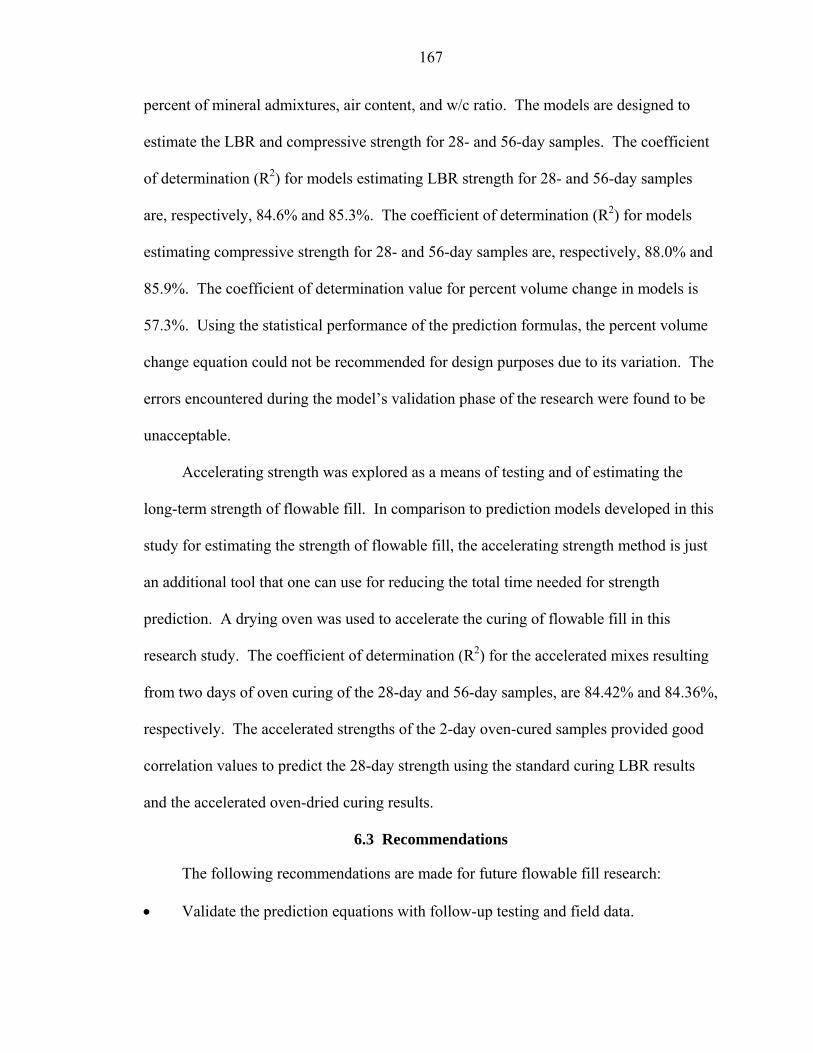
167
percent of mineral admixtures, air content, and w/c ratio. The models are designed to
estimate the LBR and compressive strength for 28- and 56-day samples. The coefficient
of determination (R2) for models estimating LBR strength for 28- and 56-day samples
are, respectively, 84.6% and 85.3%. The coefficient of determination (R2) for models
estimating compressive strength for 28- and 56-day samples are, respectively, 88.0% and
85.9%. The coefficient of determination value for percent volume change in models is
57.3%. Using the statistical performance of the prediction formulas, the percent volume
change equation could not be recommended for design purposes due to its variation. The
errors encountered during the model’s validation phase of the research were found to be
unacceptable.
Accelerating strength was explored as a means of testing and of estimating the
long-term strength of flowable fill. In comparison to prediction models developed in this
study for estimating the strength of flowable fill, the accelerating strength method is just
an additional tool that one can use for reducing the total time needed for strength
prediction. A drying oven was used to accelerate the curing of flowable fill in this
research study. The coefficient of determination (R2) for the accelerated mixes resulting
from two days of oven curing of the 28-day and 56-day samples, are 84.42% and 84.36%,
respectively. The accelerated strengths of the 2-day oven-cured samples provided good
correlation values to predict the 28-day strength using the standard curing LBR results
and the accelerated oven-dried curing results.
6.3 Recommendations
The following recommendations are made for future flowable fill research:
• Validate the prediction equations with follow-up testing and field data.

168
• Introduce the design prediction equations to DOT’s materials engineers (local, county and state), and concrete producers. Doing so will promote understanding of its usage and applications.
• Refine the related equations with field data.

169
APPENDIX A FLOWABLE FILL STUDY BATCH MIX DESIGN MATRIX
This appendix includes the design matrix (Table A-1), batch mix combinations
(Tables A-2 through A-9), typical computations of empirical mix design, and volumetric
results per batch mix used for this research study (Tables A-10 through A-13).

170
Table A-1. Full factorial design matrix
Air Content (B)
b1 b2
W/C Ratio (C)
c1 c2 c3 c1 c2 c3
Mineral Admixtures (D)
Cement Content (A)
d1 d2 d3 d1 d2 d3 d1 d2 d3 d1 d2 d3 d1 d2 d3 d1 d2 d3
a1 a1b1c1d1 a1b1c1d1
a1b1c1d2 a1b1c1d2
a1b1c1d3 a1b1c1d3
a1b1c2d1 a1b1c2d1
a1b1c2d2 a1b1c2d2
a1b1c2d3 a1b1c2d3
a1b1c3d1 a1b1c3d1
a1b1c3d2 a1b1c3d2
a1b1c3d3 a1b1c3d3
a1b2c1d1 a1b2c1d1
a1b2c1d2 a1b2c1d2
a1b2c1d3 a1b2c1d3
a1b2c2d1 a1b2c2d1
a1b2c2d2 a1b2c2d2
a1b2c2d3 a1b2c2d3
a1b2c3d1 a1b2c3d1
a1b2c3d2 a1b2c3d2
a1b2c3d3 a1b2c3d3
a2 a2b1c1d1 a2b1c1d1
a2b1c1d2 a2b1c1d2
a2b1c1d3 a2b1c1d3
a2b1c2d1 a2b1c2d1
a2b1c2d2 a2b1c2d2
a2b1c2d3 a2b1c2d3
a2b1c3d1 a2b1c3d1
a2b1c3d2 a2b1c3d2
a2b1c3d3 a2b1c3d3
a2b2c1d1 a2b2c1d1
a2b2c1d2 a2b2c1d2
a2b2c1d3 a2b2c1d3
a2b2c2d1 a2b2c2d1
a2b2c2d2 a2b2c2d2
a2b2c2d3 a2b2c2d3
a2b2c3d1 a2b2c3d1
a2b2c3d2 a2b2c3d2
a2b2c3d3 a2b2c3d3
a3 a3b1c1d1 a3b1c1d1
a3b1c1d2 a3b1c1d2
a3b1c1d3 a3b1c1d3
a3b1c2d1 a3b1c2d1
a3b1c2d2 a3b1c2d2
a3b1c2d3 a3b1c2d3
a3b1c3d1 a3b1c3d1
a3b1c3d2 a3b1c3d2
a3b1c3d3 a3b1c3d3
a3b2c1d1 a3b2c1d1
a3b2c1d2 a3b2c1d2
a3b2c1d3 a3b2c1d3
a3b2c2d1 a3b2c2d1
a3b2c2d2 a3b2c2d2
a3b2c2d3 a3b2c2d3
a3b2c3d1 a3b2c3d1
a3b2c3d2 a3b2c3d2
a3b2c3d3 a3b2c3d3
a4 a4b1c1d1 a4b1c1d1
a4b1c1d2 a4b1c1d2
a4b1c1d3 a4b1c1d3
a4b1c2d1 a4b1c2d1
a4b1c2d2 a4b1c2d2
a4b1c2d3 a4b1c2d3
a4b1c3d1 a4b1c3d1
a4b1c3d2 a4b1c3d2
a4b1c3d3 a4b1c3d3
a4b2c1d1 a4b2c1d1
a4b2c1d2 a4b2c1d2
a4b2c1d3 a4b2c1d3
a4b2c2d1 a4b2c2d1
a4b2c2d2 a4b2c2d2
a4b2c2d3 a4b2c2d3
a4b2c3d1 a4b2c3d1
a4b2c3d2 a4b2c3d2
a4b2c3d3 a4b2c3d3
Note: shaded cells represent feasible mixture combinations

171
Table A-2. Batch mix combinations 1 through 22 for Experiment 1
Random Batch Mixture Cement Air w/c Mineral
Number Number CombinationContent (lb/yd3) Content ratio
Admixtures (%)
32 1 a1b1c1d1 50.0 7.5 ± 2.5% 2.0 0
71 2 a2b1c1d1 100.0 7.5 ± 2.5% 2.0 0
47 3 a3b1c1d1 150.0 7.5 ± 2.5% 2.0 0
2 4 a4b1c1d1 200.0 7.5 ± 2.5% 2.0 0
8 5 a1b1c1d2 50.0 7.5 ± 2.5% 2.0 20
46 6 a2b1c1d2 100.0 7.5 ± 2.5% 2.0 20
20 7 a3b1c1d2 150.0 7.5 ± 2.5% 2.0 20
4 8 a4b1c1d2 200.0 7.5 ± 2.5% 2.0 20
53 9 a1b1c1d3 50.0 7.5 ± 2.5% 2.0 50
33 10 a2b1c1d3 100.0 7.5 ± 2.5% 2.0 50
3 11 a3b1c1d3 150.0 7.5 ± 2.5% 2.0 50
68 12 a4b1c1d3 200.0 7.5 ± 2.5% 2.0 50
5 13 a1b1c2d1 50.0 7.5 ± 2.5% 4.5 0
48 14 a2b1c2d1 100.0 7.5 ± 2.5% 4.5 0
21 15 a3b1c2d1 150.0 7.5 ± 2.5% 4.5 0
27 16 a4b1c2d1 200.0 7.5 ± 2.5% 4.5 0
10 17 a1b1c2d2 50.0 7.5 ± 2.5% 4.5 20
11 18 a2b1c2d2 100.0 7.5 ± 2.5% 4.5 20
56 19 a3b1c2d2 150.0 7.5 ± 2.5% 4.5 20
13 20 a4b1c2d2 200.0 7.5 ± 2.5% 4.5 20
62 21 a1b1c2d3 50.0 7.5 ± 2.5% 4.5 50
70 22 a2b1c2d3 100.0 7.5 ± 2.5% 4.5 50

172
Table A-3. Batch mix combinations 23 through 44 for Experiment 1
Random Batch Mixture Cement Air w/c Mineral
Number Number CombinationContent (lb/yd3) Content ratio
Admixtures (%)
34 23 a3b1c2d3 150.0 7.5 ± 2.5% 4.5 50
38 24 a4b1c2d3 200.0 7.5 ± 2.5% 4.5 50
6 25 a1b1c3d1 50.0 7.5 ± 2.5% 9.0 0
64 26 a2b1c3d1 100.0 7.5 ± 2.5% 9.0 0
12 27 a3b1c3d1 150.0 7.5 ± 2.5% 9.0 0
60 28 a4b1c3d1 200.0 7.5 ± 2.5% 9.0 0
15 29 a1b1c3d2 50.0 7.5 ± 2.5% 9.0 20
9 30 a2b1c3d2 100.0 7.5 ± 2.5% 9.0 20
57 31 a3b1c3d2 150.0 7.5 ± 2.5% 9.0 20
55 32 a4b1c3d2 200.0 7.5 ± 2.5% 9.0 20
16 33 a1b1c3d3 50.0 7.5 ± 2.5% 9.0 50
36 34 a2b1c3d3 100.0 7.5 ± 2.5% 9.0 50
19 35 a3b1c3d3 150.0 7.5 ± 2.5% 9.0 50
40 36 a4b1c3d3 200.0 7.5 ± 2.5% 9.0 50
39 37 a1b2c1d1 50.0 17.5 ± 2.5% 2.0 0
23 38 a2b2c1d1 100.0 17.5 ± 2.5% 2.0 0
22 39 a3b2c1d1 150.0 17.5 ± 2.5% 2.0 0
72 40 a4b2c1d1 200.0 17.5 ± 2.5% 2.0 0
28 41 a1b2c1d2 50.0 17.5 ± 2.5% 2.0 20
59 42 a2b2c1d2 100.0 17.5 ± 2.5% 2.0 20
50 43 a3b2c1d2 150.0 17.5 ± 2.5% 2.0 20
42 44 a4b2c1d2 200.0 17.5 ± 2.5% 2.0 20

173
Table A-4. Batch mix combinations 45 through 66 for Experiment 1
Random Batch Mixture Cement Air w/c Mineral
Number Number CombinationContent (lb/yd3) Content ratio
Admixtures (%)
49 45 a1b2c1d3 50.0 17.5 ± 2.5% 2.0 50
18 46 a2b2c1d3 100.0 17.5 ± 2.5% 2.0 50
52 47 a3b2c1d3 150.0 17.5 ± 2.5% 2.0 50
24 48 a4b2c1d3 200.0 17.5 ± 2.5% 2.0 50
61 49 a1b2c2d1 50.0 17.5 ± 2.5% 4.5 0
25 50 a2b2c2d1 100.0 17.5 ± 2.5% 4.5 0
51 51 a3b2c2d1 150.0 17.5 ± 2.5% 4.5 0
14 52 a4b2c2d1 200.0 17.5 ± 2.5% 4.5 0
7 53 a1b2c2d2 50.0 17.5 ± 2.5% 4.5 20
66 54 a2b2c2d2 100.0 17.5 ± 2.5% 4.5 20
67 55 a3b2c2d2 150.0 17.5 ± 2.5% 4.5 20
29 56 a4b2c2d2 200.0 17.5 ± 2.5% 4.5 20
37 57 a1b2c2d3 50.0 17.5 ± 2.5% 4.5 50
45 58 a2b2c2d3 100.0 17.5 ± 2.5% 4.5 50
43 59 a3b2c2d3 150.0 17.5 ± 2.5% 4.5 50
58 60 a4b2c2d3 200.0 17.5 ± 2.5% 4.5 50
31 61 a1b2c3d1 50.0 17.5 ± 2.5% 9.0 0
41 62 a2b2c3d1 100.0 17.5 ± 2.5% 9.0 0
63 63 a3b2c3d1 150.0 17.5 ± 2.5% 9.0 0
69 64 a4b2c3d1 200.0 17.5 ± 2.5% 9.0 0
44 65 a1b2c3d2 50.0 17.5 ± 2.5% 9.0 20
17 66 a2b2c3d2 100.0 17.5 ± 2.5% 9.0 20

174
Table A-5. Batch mix combinations 67 through 72 for Experiment 1
Random Batch Mixture Cement Air w/c Mineral
Number Number CombinationContent (lb/yd3) Content ratio
Admixtures (%)
1 67 a3b2c3d2 150.0 17.5 ± 2.5% 9.0 20
30 68 a4b2c3d2 200.0 17.5 ± 2.5% 9.0 20
54 69 a1b2c3d3 50.0 17.5 ± 2.5% 9.0 50
65 70 a2b2c3d3 100.0 17.5 ± 2.5% 9.0 50
35 71 a3b2c3d3 150.0 17.5 ± 2.5% 9.0 50
26 72 a4b2c3d3 200.0 17.5 ± 2.5% 9.0 50

175
Table A-6. Batch mix combination replicates 1r through 22r for Experiment 2
Random Batch Mixture Cement Air w/c Mineral
Number Number CombinationContent (lb/yd3) Content ratio
Admixtures (%)
6 1r a1b1c1d1 50.0 7.5 ± 2.5% 2.0 0
43 2r a2b1c1d1 100.0 7.5 ± 2.5% 2.0 0
20 3r a3b1c1d1 150.0 7.5 ± 2.5% 2.0 0
45 4r a4b1c1d1 200.0 7.5 ± 2.5% 2.0 0
66 5r a1b1c1d2 50.0 7.5 ± 2.5% 2.0 20
47 6r a2b1c1d2 100.0 7.5 ± 2.5% 2.0 20
21 7r a3b1c1d2 150.0 7.5 ± 2.5% 2.0 20
1 8r a4b1c1d2 200.0 7.5 ± 2.5% 2.0 20
58 9r a1b1c1d3 50.0 7.5 ± 2.5% 2.0 50
39 10r a2b1c1d3 100.0 7.5 ± 2.5% 2.0 50
34 11r a3b1c1d3 150.0 7.5 ± 2.5% 2.0 50
52 12r a4b1c1d3 200.0 7.5 ± 2.5% 2.0 50
25 13r a1b1c2d1 50.0 7.5 ± 2.5% 4.5 0
10 14r a2b1c2d1 100.0 7.5 ± 2.5% 4.5 0
55 15r a3b1c2d1 150.0 7.5 ± 2.5% 4.5 0
3 16r a4b1c2d1 200.0 7.5 ± 2.5% 4.5 0
35 17r a1b1c2d2 50.0 7.5 ± 2.5% 4.5 20
7 18r a2b1c2d2 100.0 7.5 ± 2.5% 4.5 20
30 19r a3b1c2d2 150.0 7.5 ± 2.5% 4.5 20
57 20r a4b1c2d2 200.0 7.5 ± 2.5% 4.5 20
9 21r a1b1c2d3 50.0 7.5 ± 2.5% 4.5 50
11 22r a2b1c2d3 100.0 7.5 ± 2.5% 4.5 50

176
Table A-7. Batch mix combination replicates 23r through 45r for Experiment 2
Random Batch Mixture Cement Air w/c Mineral
Number Number CombinationContent (lb/yd3) Content ratio
Admixtures (%)
14 23r a3b1c2d3 150.0 7.5 ± 2.5% 4.5 50
68 24r a4b1c2d3 200.0 7.5 ± 2.5% 4.5 50
16 25r a1b1c3d1 50.0 7.5 ± 2.5% 9.0 0
26 26r a2b1c3d1 100.0 7.5 ± 2.5% 9.0 0
72 27r a3b1c3d1 150.0 7.5 ± 2.5% 9.0 0
67 28r a4b1c3d1 200.0 7.5 ± 2.5% 9.0 0
48 29r a1b1c3d2 50.0 7.5 ± 2.5% 9.0 20
5 30r a2b1c3d2 100.0 7.5 ± 2.5% 9.0 20
65 31r a3b1c3d2 150.0 7.5 ± 2.5% 9.0 20
23 32r a4b1c3d2 200.0 7.5 ± 2.5% 9.0 20
12 33r a1b1c3d3 50.0 7.5 ± 2.5% 9.0 50
17 34r a2b1c3d3 100.0 7.5 ± 2.5% 9.0 50
38 35r a3b1c3d3 150.0 7.5 ± 2.5% 9.0 50
24 36r a4b1c3d3 200.0 7.5 ± 2.5% 9.0 50
2 37r a1b2c1d1 50.0 17.5 ± 2.5% 2.0 0
28 38r a2b2c1d1 100.0 17.5 ± 2.5% 2.0 0
18 39r a3b2c1d1 150.0 17.5 ± 2.5% 2.0 0
27 40r a4b2c1d1 200.0 17.5 ± 2.5% 2.0 0
31 41r a1b2c1d2 50.0 17.5 ± 2.5% 2.0 20
37 42r a2b2c1d2 100.0 17.5 ± 2.5% 2.0 20
8 43r a3b2c1d2 150.0 17.5 ± 2.5% 2.0 20
33 44r a4b2c1d2 200.0 17.5 ± 2.5% 2.0 20
32 45r a1b2c1d3 50.0 17.5 ± 2.5% 2.0 50
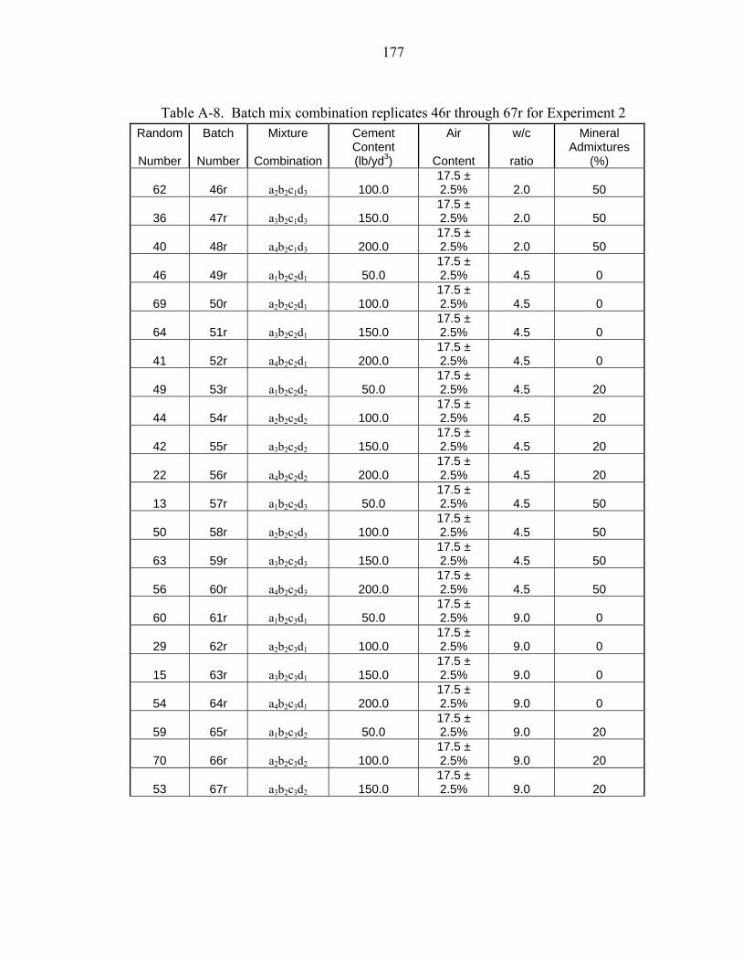
177
Table A-8. Batch mix combination replicates 46r through 67r for Experiment 2
Random Batch Mixture Cement Air w/c Mineral
Number Number CombinationContent (lb/yd3) Content ratio
Admixtures (%)
62 46r a2b2c1d3 100.0 17.5 ± 2.5% 2.0 50
36 47r a3b2c1d3 150.0 17.5 ± 2.5% 2.0 50
40 48r a4b2c1d3 200.0 17.5 ± 2.5% 2.0 50
46 49r a1b2c2d1 50.0 17.5 ± 2.5% 4.5 0
69 50r a2b2c2d1 100.0 17.5 ± 2.5% 4.5 0
64 51r a3b2c2d1 150.0 17.5 ± 2.5% 4.5 0
41 52r a4b2c2d1 200.0 17.5 ± 2.5% 4.5 0
49 53r a1b2c2d2 50.0 17.5 ± 2.5% 4.5 20
44 54r a2b2c2d2 100.0 17.5 ± 2.5% 4.5 20
42 55r a3b2c2d2 150.0 17.5 ± 2.5% 4.5 20
22 56r a4b2c2d2 200.0 17.5 ± 2.5% 4.5 20
13 57r a1b2c2d3 50.0 17.5 ± 2.5% 4.5 50
50 58r a2b2c2d3 100.0 17.5 ± 2.5% 4.5 50
63 59r a3b2c2d3 150.0 17.5 ± 2.5% 4.5 50
56 60r a4b2c2d3 200.0 17.5 ± 2.5% 4.5 50
60 61r a1b2c3d1 50.0 17.5 ± 2.5% 9.0 0
29 62r a2b2c3d1 100.0 17.5 ± 2.5% 9.0 0
15 63r a3b2c3d1 150.0 17.5 ± 2.5% 9.0 0
54 64r a4b2c3d1 200.0 17.5 ± 2.5% 9.0 0
59 65r a1b2c3d2 50.0 17.5 ± 2.5% 9.0 20
70 66r a2b2c3d2 100.0 17.5 ± 2.5% 9.0 20
53 67r a3b2c3d2 150.0 17.5 ± 2.5% 9.0 20

178
Table A-9. Batch mix combination replicates 68r through 72r for Experiment 2
Random Batch Mixture Cement Air w/c Mineral
Number Number CombinationContent (lb/yd3) Content ratio
Admixtures (%)
61 68r a4b2c3d2 200.0 17.5 ± 2.5% 9.0 20
19 69r a1b2c3d3 50.0 17.5 ± 2.5% 9.0 50
71 70r a2b2c3d3 100.0 17.5 ± 2.5% 9.0 50
4 71r a3b2c3d3 150.0 17.5 ± 2.5% 9.0 50
51 72r a4b2c3d3 200.0 17.5 ± 2.5% 9.0 50
Typical computations for mixing flowable fill In this computation, one empirical flowable fill mixture will be design using the volumetric method discussed in chapter 3. The following outlined the steps used for designing 1 cubic yard (yd3) mixture:
Determine the amount of materials required for mixtures with the following design criteria:
Batch Mix #23 • cementitious content = 150 lb/yd3 • w/c = 4.50 • air content = 7.5 ± 2.5% • mineral admixtures = 50% slag
The following are known properties for the materials that will be used to create the mixtures:
Sc = 3.15 specific gravity of cement Ss = 2.42 specific gravity of slag Sf = 2.36 specific gravity of fly ash Sag = 2.63 specific gravity of fine aggregate N = 3.00 percent of natural moisture content for fine aggregate L = 0.40 percent absorption for fine aggregate Solution for batch mix #23
1. Calculate weight of cement, lbs. per cubic yard (cu. yd.)
00.7550.0150 =×=
×= pw ScontentuscementitioC

179
2. Calculate weight of slag, lbs. per cu. yd
00.7500.75150 =−=
−= ww CcontentuscementitioS
3. Calculate weight of water, lbs. per cu. yard (cu. yd.)
( )
( ) 00.67500.7500.7550.4
/
=+×=
+×= www SCratiocwW
4. Calculate absolute volume of cement, cu. ft. per cu. yd.
3382.0
4.6215.300.75
4.62ft
SC
Cc
wv =
×=
×=
5. Calculate absolute volume of slag, cu. ft. per cu. yd.
3497.0
4.6242.200.75
4.62ft
SS
Ss
wv =
×=
×=
6. Calculate absolute volume of water, cu. ft. per cu. yd.
3817.10
4.6200.675
4.62ft
WW w
v ===
7. Calculate absolute volume of target air content, cu. ft. per cu. yd.
3025.2
100275.7
10027
ftA
A pv =
×=
×=
8. Calculate total absolute volume of know ingredients
3721.13 ftAWSC vvvv =+++
9. Calculate absolute volume of saturated-surface-dry (SSD) fine aggregates,
cu. ft. per cu. yd.
3279.13)(27 ftAWSCFA vvvvvs =+++−=

180
10. Calculate weight of saturated-surface-dry fine aggregates, lbs. per cu. yd.
24.21794.6263.2279.13
4.62
=××=
××= agvsws SFAFA
11. Calculate the sand to water (s/w) ratio (s/w ratio range: 1.73 – 7.20)
229.300.67524.2179
===w
ws
WFA
WS
12. Calculate weight of fine aggregate base on natural moisture content, lbs. per
cu. yd.
67.2235004.0103.0124.2179
11
=++
×=
++
×=LNFAFA wswn
13. Correct the weight of water content due to percentage of moisture difference,
lbs. per cu. yd.
43.73143.5600.675
43.5624.217967.2235
=+=
Δ+=
=−=−=Δ
W
WWW
FAFAW
w
wnws
A summary of materials required for mixtures is provided in Tables A-10 through
A-13.

181
Table A-10. Volume computation results for batch mixes 1 through 36
Volume of Batch = 1.0 yd3 Volume of Batch = 5.50 ft3
Random Batch Weight of Weight of Weight of Weight of Weight of Weight of Weight of Weight of Weight of Weight of sand/waterNumber Number Cement (lbs) Slag (lbs) Fly Ash (lbs) Water (lbs) Fine Aggregate (lbs) Cement (lbs) Slag (lbs) Fly Ash (lbs) Water (lbs) Fine Aggregate (lbs) ratio
32 1 50.00 0.00 0.00 100.00 lbs 3793.95 lbs 10.19 0.00 0.00 20.37 lbs 772.84 lbs 37.9471 2 100.00 0.00 0.00 200.00 lbs 3489.21 lbs 20.37 0.00 0.00 40.74 lbs 710.76 lbs 17.4547 3 150.00 0.00 0.00 300.00 lbs 3184.46 lbs 30.56 0.00 0.00 61.11 lbs 648.69 lbs 10.612 4 200.00 0.00 0.00 400.00 lbs 2879.71 lbs 40.74 0.00 0.00 81.48 lbs 586.61 lbs 7.208 5 40.00 0.00 10.00 100.00 lbs 3791.16 lbs 8.15 0.00 2.04 20.37 lbs 772.27 lbs 37.91
46 6 80.00 0.00 20.00 200.00 lbs 3483.62 lbs 16.30 0.00 4.07 40.74 lbs 709.63 lbs 17.4220 7 120.00 0.00 30.00 300.00 lbs 3176.07 lbs 24.44 0.00 6.11 61.11 lbs 646.98 lbs 10.594 8 160.00 0.00 40.00 400.00 lbs 2868.53 lbs 32.59 0.00 8.15 81.48 lbs 584.33 lbs 7.17
53 9 25.00 25.00 0.00 100.00 lbs 3792.31 lbs 5.09 5.09 0.00 20.37 lbs 772.51 lbs 37.9233 10 50.00 50.00 0.00 200.00 lbs 3485.92 lbs 10.19 10.19 0.00 40.74 lbs 710.09 lbs 17.433 11 75.00 75.00 0.00 300.00 lbs 3179.53 lbs 15.28 15.28 0.00 61.11 lbs 647.68 lbs 10.60
68 12 100.00 100.00 0.00 400.00 lbs 2873.14 lbs 20.37 20.37 0.00 81.48 lbs 585.27 lbs 7.185 13 50.00 0.00 0.00 225.00 lbs 3465.20 lbs 10.19 0.00 0.00 45.83 lbs 705.87 lbs 15.40
48 14 100.00 0.00 0.00 450.00 lbs 2831.71 lbs 20.37 0.00 0.00 91.67 lbs 576.83 lbs 6.2921 15 150.00 0.00 0.00 675.00 lbs 2198.21 lbs 30.56 0.00 0.00 137.50 lbs 447.78 lbs 3.2627 16 200.00 0.00 0.00 900.00 lbs 1564.71 lbs 40.74 0.00 0.00 183.33 lbs 318.74 lbs 1.7410 17 40.00 0.00 10.00 225.00 lbs 3462.41 lbs 8.15 0.00 2.04 45.83 lbs 705.30 lbs 15.3911 18 80.00 0.00 20.00 450.00 lbs 2826.12 lbs 16.30 0.00 4.07 91.67 lbs 575.69 lbs 6.2856 19 120.00 0.00 30.00 675.00 lbs 2189.82 lbs 24.44 0.00 6.11 137.50 lbs 446.08 lbs 3.2413 20 160.00 0.00 40.00 900.00 lbs 1553.53 lbs 32.59 0.00 8.15 183.33 lbs 316.46 lbs 1.7362 21 25.00 25.00 0.00 225.00 lbs 3463.56 lbs 5.09 5.09 0.00 45.83 lbs 705.54 lbs 15.3970 22 50.00 50.00 0.00 450.00 lbs 2828.42 lbs 10.19 10.19 0.00 91.67 lbs 576.16 lbs 6.2934 23 75.00 75.00 0.00 675.00 lbs 2193.28 lbs 15.28 15.28 0.00 137.50 lbs 446.78 lbs 3.2538 24 100.00 100.00 0.00 900.00 lbs 1558.14 lbs 20.37 20.37 0.00 183.33 lbs 317.40 lbs 1.736 25 50.00 0.00 0.00 450.00 lbs 2873.45 lbs 10.19 0.00 0.00 91.67 lbs 585.33 lbs 6.39
64 26 100.00 0.00 0.00 900.00 lbs 1648.21 lbs 20.37 0.00 0.00 183.33 lbs 335.75 lbs 1.8312 27 150.00 0.00 0.00 1350.00 lbs 422.96 lbs 30.56 0.00 0.00 275.00 lbs 86.16 lbs 0.3160 28 200.00 0.00 0.00 1800.00 lbs -802.29 lbs 40.74 0.00 0.00 366.67 lbs -163.43 lbs -0.4515 29 40.00 0.00 10.00 450.00 lbs 2870.66 lbs 8.15 0.00 2.04 91.67 lbs 584.76 lbs 6.389 30 80.00 0.00 20.00 900.00 lbs 1642.62 lbs 16.30 0.00 4.07 183.33 lbs 334.61 lbs 1.83
57 31 120.00 0.00 30.00 1350.00 lbs 414.57 lbs 24.44 0.00 6.11 275.00 lbs 84.45 lbs 0.3155 32 160.00 0.00 40.00 1800.00 lbs -813.47 lbs 32.59 0.00 8.15 366.67 lbs -165.71 lbs -0.4516 33 25.00 25.00 0.00 450.00 lbs 2871.81 lbs 5.09 5.09 0.00 91.67 lbs 585.00 lbs 6.3836 34 50.00 50.00 0.00 900.00 lbs 1644.92 lbs 10.19 10.19 0.00 183.33 lbs 335.08 lbs 1.8319 35 75.00 75.00 0.00 1350.00 lbs 418.03 lbs 15.28 15.28 0.00 275.00 lbs 85.15 lbs 0.3140 36 100.00 100.00 0.00 1800.00 lbs -808.86 lbs 20.37 20.37 0.00 366.67 lbs -164.77 lbs -0.45

182
Table A-11. Volume computation results for batch mixes 37 through 72
Volume of Batch = 1.0 yd3 Volume of Batch = 5.50 ft3
Random Batch Weight of Weight of Weight of Weight of Weight of Weight of Weight of Weight of Weight of Weight of sand/waterNumber Number Cement (lbs) Slag (lbs) Fly Ash (lbs) Water (lbs) Fine Aggregate (lbs) Cement (lbs) Slag (lbs) Fly Ash (lbs) Water (lbs) Fine Aggregate (lbs) ratio
39 37 50.00 0.00 0.00 100.00 lbs 3350.85 lbs 10.19 0.00 0.00 20.37 lbs 682.58 lbs 33.5123 38 100.00 0.00 0.00 200.00 lbs 3046.10 lbs 20.37 0.00 0.00 40.74 lbs 620.50 lbs 15.2322 39 150.00 0.00 0.00 300.00 lbs 2741.36 lbs 30.56 0.00 0.00 61.11 lbs 558.42 lbs 9.1472 40 200.00 0.00 0.00 400.00 lbs 2436.61 lbs 40.74 0.00 0.00 81.48 lbs 496.35 lbs 6.0928 41 40.00 0.00 10.00 100.00 lbs 3348.05 lbs 8.15 0.00 2.04 20.37 lbs 682.01 lbs 33.4859 42 80.00 0.00 20.00 200.00 lbs 3040.51 lbs 16.30 0.00 4.07 40.74 lbs 619.36 lbs 15.2050 43 120.00 0.00 30.00 300.00 lbs 2732.97 lbs 24.44 0.00 6.11 61.11 lbs 556.72 lbs 9.1142 44 160.00 0.00 40.00 400.00 lbs 2425.43 lbs 32.59 0.00 8.15 81.48 lbs 494.07 lbs 6.0649 45 25.00 25.00 0.00 100.00 lbs 3349.20 lbs 5.09 5.09 0.00 20.37 lbs 682.25 lbs 33.4918 46 50.00 50.00 0.00 200.00 lbs 3042.81 lbs 10.19 10.19 0.00 40.74 lbs 619.83 lbs 15.2152 47 75.00 75.00 0.00 300.00 lbs 2736.42 lbs 15.28 15.28 0.00 61.11 lbs 557.42 lbs 9.1224 48 100.00 100.00 0.00 400.00 lbs 2430.03 lbs 20.37 20.37 0.00 81.48 lbs 495.01 lbs 6.0861 49 50.00 0.00 0.00 225.00 lbs 3022.10 lbs 10.19 0.00 0.00 45.83 lbs 615.61 lbs 13.4325 50 100.00 0.00 0.00 450.00 lbs 2388.60 lbs 20.37 0.00 0.00 91.67 lbs 486.57 lbs 5.3151 51 150.00 0.00 0.00 675.00 lbs 1755.11 lbs 30.56 0.00 0.00 137.50 lbs 357.52 lbs 2.6014 52 200.00 0.00 0.00 900.00 lbs 1121.61 lbs 40.74 0.00 0.00 183.33 lbs 228.48 lbs 1.257 53 40.00 0.00 10.00 225.00 lbs 3019.30 lbs 8.15 0.00 2.04 45.83 lbs 615.04 lbs 13.42
66 54 80.00 0.00 20.00 450.00 lbs 2383.01 lbs 16.30 0.00 4.07 91.67 lbs 485.43 lbs 5.3067 55 120.00 0.00 30.00 675.00 lbs 1746.72 lbs 24.44 0.00 6.11 137.50 lbs 355.81 lbs 2.5929 56 160.00 0.00 40.00 900.00 lbs 1110.43 lbs 32.59 0.00 8.15 183.33 lbs 226.20 lbs 1.2337 57 25.00 25.00 0.00 225.00 lbs 3020.45 lbs 5.09 5.09 0.00 45.83 lbs 615.28 lbs 13.4245 58 50.00 50.00 0.00 450.00 lbs 2385.31 lbs 10.19 10.19 0.00 91.67 lbs 485.90 lbs 5.3043 59 75.00 75.00 0.00 675.00 lbs 1750.17 lbs 15.28 15.28 0.00 137.50 lbs 356.52 lbs 2.5958 60 100.00 100.00 0.00 900.00 lbs 1115.03 lbs 20.37 20.37 0.00 183.33 lbs 227.14 lbs 1.2431 61 50.00 0.00 0.00 450.00 lbs 2430.35 lbs 10.19 0.00 0.00 91.67 lbs 495.07 lbs 5.4041 62 100.00 0.00 0.00 900.00 lbs 1205.10 lbs 20.37 0.00 0.00 183.33 lbs 245.48 lbs 1.3463 63 150.00 0.00 0.00 1350.00 lbs -20.14 lbs 30.56 0.00 0.00 275.00 lbs -4.10 lbs -0.0169 64 200.00 0.00 0.00 1800.00 lbs -1245.39 lbs 40.74 0.00 0.00 366.67 lbs -253.69 lbs -0.6944 65 40.00 0.00 10.00 450.00 lbs 2427.55 lbs 8.15 0.00 2.04 91.67 lbs 494.50 lbs 5.3917 66 80.00 0.00 20.00 900.00 lbs 1199.51 lbs 16.30 0.00 4.07 183.33 lbs 244.35 lbs 1.331 67 120.00 0.00 30.00 1350.00 lbs -28.53 lbs 24.44 0.00 6.11 275.00 lbs -5.81 lbs -0.02
30 68 160.00 0.00 40.00 1800.00 lbs -1256.57 lbs 32.59 0.00 8.15 366.67 lbs -255.97 lbs -0.7054 69 25.00 25.00 0.00 450.00 lbs 2428.70 lbs 5.09 5.09 0.00 91.67 lbs 494.74 lbs 5.4065 70 50.00 50.00 0.00 900.00 lbs 1201.81 lbs 10.19 10.19 0.00 183.33 lbs 244.81 lbs 1.3435 71 75.00 75.00 0.00 1350.00 lbs -25.08 lbs 15.28 15.28 0.00 275.00 lbs -5.11 lbs -0.0226 72 100.00 100.00 0.00 1800.00 lbs -1251.97 lbs 20.37 20.37 0.00 366.67 lbs -255.03 lbs -0.70

183
Table A-12. Volume computation results for replicate batch mixes 1r through 36r
Volume of Batch = 1.0 yd3 Volume of Batch = 5.50 ft3
Random Batch Weight of Weight of Weight of Weight of Weight of Weight of Weight of Weight of Weight of Weight of sand/waterNumber Number Cement (lbs) Slag (lbs) Fly Ash (lbs) Water (lbs) Fine Aggregate (lbs) Cement (lbs) Slag (lbs) Fly Ash (lbs) Water (lbs) Fine Aggregate (lbs) ratio
6 1r 50.00 0.00 0.00 100.00 lbs 3793.95 lbs 10.19 0.00 0.00 20.37 lbs 772.84 lbs 37.9443 2r 100.00 0.00 0.00 200.00 lbs 3489.21 lbs 20.37 0.00 0.00 40.74 lbs 710.76 lbs 17.4520 3r 150.00 0.00 0.00 300.00 lbs 3184.46 lbs 30.56 0.00 0.00 61.11 lbs 648.69 lbs 10.6145 4r 200.00 0.00 0.00 400.00 lbs 2879.71 lbs 40.74 0.00 0.00 81.48 lbs 586.61 lbs 7.2066 5r 40.00 0.00 10.00 100.00 lbs 3791.16 lbs 8.15 0.00 2.04 20.37 lbs 772.27 lbs 37.9147 6r 80.00 0.00 20.00 200.00 lbs 3483.62 lbs 16.30 0.00 4.07 40.74 lbs 709.63 lbs 17.4221 7r 120.00 0.00 30.00 300.00 lbs 3176.07 lbs 24.44 0.00 6.11 61.11 lbs 646.98 lbs 10.591 8r 160.00 0.00 40.00 400.00 lbs 2868.53 lbs 32.59 0.00 8.15 81.48 lbs 584.33 lbs 7.17
58 9r 25.00 25.00 0.00 100.00 lbs 3792.31 lbs 5.09 5.09 0.00 20.37 lbs 772.51 lbs 37.9239 10r 50.00 50.00 0.00 200.00 lbs 3485.92 lbs 10.19 10.19 0.00 40.74 lbs 710.09 lbs 17.4334 11r 75.00 75.00 0.00 300.00 lbs 3179.53 lbs 15.28 15.28 0.00 61.11 lbs 647.68 lbs 10.6052 12r 100.00 100.00 0.00 400.00 lbs 2873.14 lbs 20.37 20.37 0.00 81.48 lbs 585.27 lbs 7.1825 13r 50.00 0.00 0.00 225.00 lbs 3465.20 lbs 10.19 0.00 0.00 45.83 lbs 705.87 lbs 15.4010 14r 100.00 0.00 0.00 450.00 lbs 2831.71 lbs 20.37 0.00 0.00 91.67 lbs 576.83 lbs 6.2955 15r 150.00 0.00 0.00 675.00 lbs 2198.21 lbs 30.56 0.00 0.00 137.50 lbs 447.78 lbs 3.263 16r 200.00 0.00 0.00 900.00 lbs 1564.71 lbs 40.74 0.00 0.00 183.33 lbs 318.74 lbs 1.74
35 17r 40.00 0.00 10.00 225.00 lbs 3462.41 lbs 8.15 0.00 2.04 45.83 lbs 705.30 lbs 15.397 18r 80.00 0.00 20.00 450.00 lbs 2826.12 lbs 16.30 0.00 4.07 91.67 lbs 575.69 lbs 6.28
30 19r 120.00 0.00 30.00 675.00 lbs 2189.82 lbs 24.44 0.00 6.11 137.50 lbs 446.08 lbs 3.2457 20r 160.00 0.00 40.00 900.00 lbs 1553.53 lbs 32.59 0.00 8.15 183.33 lbs 316.46 lbs 1.739 21r 25.00 25.00 0.00 225.00 lbs 3463.56 lbs 5.09 5.09 0.00 45.83 lbs 705.54 lbs 15.39
11 22r 50.00 50.00 0.00 450.00 lbs 2828.42 lbs 10.19 10.19 0.00 91.67 lbs 576.16 lbs 6.2914 23r 75.00 75.00 0.00 675.00 lbs 2193.28 lbs 15.28 15.28 0.00 137.50 lbs 446.78 lbs 3.2568 24r 100.00 100.00 0.00 900.00 lbs 1558.14 lbs 20.37 20.37 0.00 183.33 lbs 317.40 lbs 1.7316 25r 50.00 0.00 0.00 450.00 lbs 2873.45 lbs 10.19 0.00 0.00 91.67 lbs 585.33 lbs 6.3926 26r 100.00 0.00 0.00 900.00 lbs 1648.21 lbs 20.37 0.00 0.00 183.33 lbs 335.75 lbs 1.8372 27r 150.00 0.00 0.00 1350.00 lbs 422.96 lbs 30.56 0.00 0.00 275.00 lbs 86.16 lbs 0.3167 28r 200.00 0.00 0.00 1800.00 lbs -802.29 lbs 40.74 0.00 0.00 366.67 lbs -163.43 lbs -0.4548 29r 40.00 0.00 10.00 450.00 lbs 2870.66 lbs 8.15 0.00 2.04 91.67 lbs 584.76 lbs 6.385 30r 80.00 0.00 20.00 900.00 lbs 1642.62 lbs 16.30 0.00 4.07 183.33 lbs 334.61 lbs 1.83
65 31r 120.00 0.00 30.00 1350.00 lbs 414.57 lbs 24.44 0.00 6.11 275.00 lbs 84.45 lbs 0.3123 32r 160.00 0.00 40.00 1800.00 lbs -813.47 lbs 32.59 0.00 8.15 366.67 lbs -165.71 lbs -0.4512 33r 25.00 25.00 0.00 450.00 lbs 2871.81 lbs 5.09 5.09 0.00 91.67 lbs 585.00 lbs 6.3817 34r 50.00 50.00 0.00 900.00 lbs 1644.92 lbs 10.19 10.19 0.00 183.33 lbs 335.08 lbs 1.8338 35r 75.00 75.00 0.00 1350.00 lbs 418.03 lbs 15.28 15.28 0.00 275.00 lbs 85.15 lbs 0.3124 36r 100.00 100.00 0.00 1800.00 lbs -808.86 lbs 20.37 20.37 0.00 366.67 lbs -164.77 lbs -0.45

184
Table A-13. Volume computation results for batch mixes 37r through 72r
Volume of Batch = 1.0 yd3 Volume of Batch = 5.50 ft3
Random Batch Weight of Weight of Weight of Weight of Weight of Weight of Weight of Weight of Weight of Weight of sand/waterNumber Number Cement (lbs) Slag (lbs) Fly Ash (lbs) Water (lbs) Fine Aggregate (lbs) Cement (lbs) Slag (lbs) Fly Ash (lbs) Water (lbs) Fine Aggregate (lbs) ratio
2 37r 50.00 0.00 0.00 100.00 lbs 3350.85 lbs 10.19 0.00 0.00 20.37 lbs 682.58 lbs 33.5128 38r 100.00 0.00 0.00 200.00 lbs 3046.10 lbs 20.37 0.00 0.00 40.74 lbs 620.50 lbs 15.2318 39r 150.00 0.00 0.00 300.00 lbs 2741.36 lbs 30.56 0.00 0.00 61.11 lbs 558.42 lbs 9.1427 40r 200.00 0.00 0.00 400.00 lbs 2436.61 lbs 40.74 0.00 0.00 81.48 lbs 496.35 lbs 6.0931 41r 40.00 0.00 10.00 100.00 lbs 3348.05 lbs 8.15 0.00 2.04 20.37 lbs 682.01 lbs 33.4837 42r 80.00 0.00 20.00 200.00 lbs 3040.51 lbs 16.30 0.00 4.07 40.74 lbs 619.36 lbs 15.208 43r 120.00 0.00 30.00 300.00 lbs 2732.97 lbs 24.44 0.00 6.11 61.11 lbs 556.72 lbs 9.11
33 44r 160.00 0.00 40.00 400.00 lbs 2425.43 lbs 32.59 0.00 8.15 81.48 lbs 494.07 lbs 6.0632 45r 25.00 25.00 0.00 100.00 lbs 3349.20 lbs 5.09 5.09 0.00 20.37 lbs 682.25 lbs 33.4962 46r 50.00 50.00 0.00 200.00 lbs 3042.81 lbs 10.19 10.19 0.00 40.74 lbs 619.83 lbs 15.2136 47r 75.00 75.00 0.00 300.00 lbs 2736.42 lbs 15.28 15.28 0.00 61.11 lbs 557.42 lbs 9.1240 48r 100.00 100.00 0.00 400.00 lbs 2430.03 lbs 20.37 20.37 0.00 81.48 lbs 495.01 lbs 6.0846 49r 50.00 0.00 0.00 225.00 lbs 3022.10 lbs 10.19 0.00 0.00 45.83 lbs 615.61 lbs 13.4369 50r 100.00 0.00 0.00 450.00 lbs 2388.60 lbs 20.37 0.00 0.00 91.67 lbs 486.57 lbs 5.3164 51r 150.00 0.00 0.00 675.00 lbs 1755.11 lbs 30.56 0.00 0.00 137.50 lbs 357.52 lbs 2.6041 52r 200.00 0.00 0.00 900.00 lbs 1121.61 lbs 40.74 0.00 0.00 183.33 lbs 228.48 lbs 1.2549 53r 40.00 0.00 10.00 225.00 lbs 3019.30 lbs 8.15 0.00 2.04 45.83 lbs 615.04 lbs 13.4244 54r 80.00 0.00 20.00 450.00 lbs 2383.01 lbs 16.30 0.00 4.07 91.67 lbs 485.43 lbs 5.3042 55r 120.00 0.00 30.00 675.00 lbs 1746.72 lbs 24.44 0.00 6.11 137.50 lbs 355.81 lbs 2.5922 56r 160.00 0.00 40.00 900.00 lbs 1110.43 lbs 32.59 0.00 8.15 183.33 lbs 226.20 lbs 1.2313 57r 25.00 25.00 0.00 225.00 lbs 3020.45 lbs 5.09 5.09 0.00 45.83 lbs 615.28 lbs 13.4250 58r 50.00 50.00 0.00 450.00 lbs 2385.31 lbs 10.19 10.19 0.00 91.67 lbs 485.90 lbs 5.3063 59r 75.00 75.00 0.00 675.00 lbs 1750.17 lbs 15.28 15.28 0.00 137.50 lbs 356.52 lbs 2.5956 60r 100.00 100.00 0.00 900.00 lbs 1115.03 lbs 20.37 20.37 0.00 183.33 lbs 227.14 lbs 1.2460 61r 50.00 0.00 0.00 450.00 lbs 2430.35 lbs 10.19 0.00 0.00 91.67 lbs 495.07 lbs 5.4029 62r 100.00 0.00 0.00 900.00 lbs 1205.10 lbs 20.37 0.00 0.00 183.33 lbs 245.48 lbs 1.3415 63r 150.00 0.00 0.00 1350.00 lbs -20.14 lbs 30.56 0.00 0.00 275.00 lbs -4.10 lbs -0.0154 64r 200.00 0.00 0.00 1800.00 lbs -1245.39 lbs 40.74 0.00 0.00 366.67 lbs -253.69 lbs -0.6959 65r 40.00 0.00 10.00 450.00 lbs 2427.55 lbs 8.15 0.00 2.04 91.67 lbs 494.50 lbs 5.3970 66r 80.00 0.00 20.00 900.00 lbs 1199.51 lbs 16.30 0.00 4.07 183.33 lbs 244.35 lbs 1.3353 67r 120.00 0.00 30.00 1350.00 lbs -28.53 lbs 24.44 0.00 6.11 275.00 lbs -5.81 lbs -0.0261 68r 160.00 0.00 40.00 1800.00 lbs -1256.57 lbs 32.59 0.00 8.15 366.67 lbs -255.97 lbs -0.7019 69r 25.00 25.00 0.00 450.00 lbs 2428.70 lbs 5.09 5.09 0.00 91.67 lbs 494.74 lbs 5.4071 70r 50.00 50.00 0.00 900.00 lbs 1201.81 lbs 10.19 10.19 0.00 183.33 lbs 244.81 lbs 1.344 71r 75.00 75.00 0.00 1350.00 lbs -25.08 lbs 15.28 15.28 0.00 275.00 lbs -5.11 lbs -0.02
51 72r 100.00 100.00 0.00 1800.00 lbs -1251.97 lbs 20.37 20.37 0.00 366.67 lbs -255.03 lbs -0.70

185
APPENDIX B LBR AND COMPRESSIVE STRENGTH DATA
OBTAINED IN THE LABORATORY
This appendix includes plot for the bearing strength in LBR and the compressive
strength (stress) versus time for all laboratory mixes. Proctor penetrometer resistance
showing the setting behavior for all batch mixtures are provided in the tables. In addition,
tables are provided showing the individual LBR reading for the 2-days oven samples.

186
BEARING STRENGTH (LBR) vs TIME FLOWABLE FILL 2005 (BATCH MIX 4)
0
50
100
150
200
250
0 20 40 60
TIME(DAYS)
STR
ENG
TH(L
BR
)
BM 4
BM 4a
BM 4r
BEARING STRENGTH (LBR) vs TIME FLOWABLE FILL 2005 (BATCH MIX 8)
0
50
100
150
200
250
0 20 40 60
TIME(DAYS)
STR
ENG
TH(L
BR
)
BM 8
BM 8r
BEARING STRENGTH (LBR) vs TIME FLOWABLE FILL 2005 (BATCH MIX 12)
0
50
100
150
200
250
0 20 40 60
TIME(DAYS)
STR
ENG
TH(L
BR
)
BM 12
BM 12r
BEARING STRENGTH (LBR) vs TIME FLOWABLE FILL 2005 (BATCH MIX 14)
0
50
100
150
200
250
0 20 40 60
TIME(DAYS)
STR
ENG
TH(L
BR
)
BM 14
BM 14r
UnConfined Compressive Stress vs TIME FLOWABLE FILL 2005 (BATCH MIX 4)
0.00
50.00
100.00
150.00
200.00
250.00
0 20 40 60
TIME(DAYS)
STR
ESS(
PSI) BM 4
BM 4a
BM 4r
UnConfined Compressive Stress vs TIME FLOWABLE FILL 2005 (BATCH MIX 12)
0.00
50.00
100.00
150.00
200.00
250.00
0 20 40 60
TIME(DAYS)
STR
ESS(
PSI)
BM 12
BM 12r
UnConfined Compressive Stress vs TIME FLOWABLE FILL 2005 (BATCH MIX 8)
0.00
50.00
100.00
150.00
200.00
250.00
0 20 40 60
TIME(DAYS)
STR
ESS(
PSI)
BM 8
BM 8r
UnConfined Compressive Stress vs TIME FLOWABLE FILL 2005 (BATCH MIX 14)
0.00
50.00
100.00
150.00
200.00
250.00
0 20 40 60
TIME(DAYS)
STR
ESS(
PSI)
BM 14
BM 14r
Figure B-1. Batch mix 4 through batch mix 14 bearing strength, and compressive strength versus time

187
BEARING STRENGTH (LBR) vs TIME FLOWABLE FILL 2005 (BATCH MIX15)
0
50
100
150
200
250
0 20 40 60
TIME(DAYS)
STR
ENG
TH(L
BR
)BM 15
BM 15-Type I
BM 15r
BEARING STRENGTH (LBR) vs TIME FLOWABLE FILL 2005 (BATCH MIX 16)
050
100150200250300350
0 20 40 60
TIME(DAYS)
STR
ENG
TH(L
BR
)
BM 16
BM 16a
BM 16r
BEARING STRENGTH (LBR) vs TIME FLOWABLE FILL 2005 (BATCH MIX 18)
0
50
100
150
200
250
0 20 40 60
TIME(DAYS)
STR
ENG
TH(L
BR
)
BM 18
BM 18r
BEARING STRENGTH (LBR) vs TIME FLOWABLE FILL 2005 (BATCH MIX 19)
0
50
100
150
200
250
0 20 40 60
TIME(DAYS)
STR
ENG
TH(L
BR
)
BM 19
BM 19r
UnConfined Compressive Stress vs TIME FLOWABLE FILL 2005 (BATCH MIX15)
0.00
50.00
100.00
150.00
200.00
250.00
0 20 40 60
TIME(DAYS)
STR
ESS(
PSI) BM 15
BM 15-Type I
BM 15r
UnConfined Compressive Stress vs TIME FLOWABLE FILL 2005 (BATCH MIX 18)
0.00
50.00
100.00
150.00
200.00
250.00
0 20 40 60
TIME(DAYS)
STR
ESS(
PSI)
BM 18
BM 18r
UnConfined Compressive Stress vs TIME FLOWABLE FILL 2005 (BATCH MIX 16)
0.00
50.00
100.00
150.00
200.00
250.00
0 20 40 60
TIME(DAYS)
STR
ESS(
PSI) BM 16
BM 16a
BM 16r
UnConfined Compressive Stress vs TIME FLOWABLE FILL 2005 (BATCH MIX 19)
0.00
50.00
100.00
150.00
200.00
250.00
0 20 40 60
TIME(DAYS)
STR
ESS(
PSI)
BM 19
BM 19r
Figure B-2. Batch mix 15 through batch mix 19 bearing strength, and compressive strength versus time

188
BEARING STRENGTH (LBR) vs TIME FLOWABLE FILL 2005 (BATCH MIX 20)
0
50
100
150
200
250
0 20 40 60
TIME(DAYS)
STR
ENG
TH(L
BR
)
BM 20
BM 20r
BEARING STRENGTH (LBR) vs TIME FLOWABLE FILL 2005 (BATCH MIX 22)
0
50
100
150
200
250
0 20 40 60
TIME(DAYS)
STR
ENG
TH(L
BR
)
BM 22
BM 22r
BEARING STRENGTH (LBR) vs TIME FLOWABLE FILL 2005 (BATCH MIX 23)
0
50
100
150
200
250
0 20 40 60
TIME(DAYS)
STR
ENG
TH(L
BR
)
BM 23
BM 23r
BEARING STRENGTH (LBR) vs TIME FLOWABLE FILL 2005 (BATCH MIX 24)
0
50
100
150
200
250
300
0 20 40 60
TIME(DAYS)
STR
ENG
TH(L
BR
)
BM 24
BM 24r
UnConfined Compressive Stress vs TIME FLOWABLE FILL 2005 (BATCH MIX 20)
0.00
50.00
100.00
150.00
200.00
250.00
0 20 40 60
TIME(DAYS)
STR
ESS(
PSI)
BM 20
BM 20r
UnConfined Compressive Stress vs TIME FLOWABLE FILL 2005 (BATCH MIX 23)
0.00
50.00
100.00
150.00
200.00
250.00
0 20 40 60
TIME(DAYS)
STR
ESS(
PSI)
BM 23
BM 23r
UnConfined Compressive Stress vs TIME FLOWABLE FILL 2005 (BATCH MIX 22)
0.00
50.00
100.00
150.00
200.00
250.00
0 20 40 60
TIME(DAYS)
STR
ESS(
PSI)
BM 22
BM 22r
UnConfined Compressive Stress vs TIME FLOWABLE FILL 2005 (BATCH MIX 24)
0.00
50.00
100.00
150.00
200.00
250.00
0 20 40 60
TIME(DAYS)
STR
ESS(
PSI)
BM 24
BM 24r
Figure B-3. Batch mix 20 through batch mix 24 bearing strength, and compressive strength versus time

189
BEARING STRENGTH (LBR) vs TIME FLOWABLE FILL 2005 (BATCH MIX 25)
0
50
100
150
200
250
0 20 40 60
TIME(DAYS)
STR
ENG
TH(L
BR
)BM 25
BM 25-Type IBM 25r
BM 25rb
BEARING STRENGTH (LBR) vs TIME FLOWABLE FILL 2005 (BATCH MIX 26)
0
50
100
150
200
250
0 20 40 60
TIME(DAYS)
STR
ENG
TH(L
BR
)
BM 26
BM 26r
BEARING STRENGTH (LBR) vs TIME FLOWABLE FILL 2005 (BATCH MIX 30)
0
50
100
150
200
250
0 20 40 60
TIME(DAYS)
STR
ENG
TH(L
BR
)
BM 30
BM 30r
BEARING STRENGTH (LBR) vs TIME FLOWABLE FILL 2005 (BATCH MIX 33)
0
50
100
150
200
250
0 20 40 60
TIME(DAYS)
STR
ENG
TH(L
BR
)
BM 33
BM 33r
UnConfined Compressive Stress vs TIME FLOWABLE FILL 2005 (BATCH MIX 25)
0.00
50.00
100.00
150.00
200.00
250.00
0 20 40 60
TIME(DAYS)
STR
ESS(
PSI) BM 25
BM 25-Type IBM 25r
BM 25rb
UnConfined Compressive Stress vs TIME FLOWABLE FILL 2005 (BATCH MIX 30)
0.00
50.00
100.00
150.00
200.00
250.00
0 20 40 60
TIME(DAYS)
STR
ESS(
PSI)
BM 30
BM 30r
UnConfined Compressive Stress vs TIME FLOWABLE FILL 2005 (BATCH MIX 26)
0.00
50.00
100.00
150.00
200.00
250.00
0 20 40 60
TIME(DAYS)
STR
ESS(
PSI)
BM 26
BM 26r
UnConfined Compressive Stress vs TIME FLOWABLE FILL 2005 (BATCH MIX 33)
0.00
50.00
100.00
150.00
200.00
250.00
0 20 40 60
TIME(DAYS)
STR
ESS(
PSI)
BM 33
BM 33r
Figure B-4. Batch mix 25 through batch mix 33 bearing strength, and compressive strength versus time

190
BEARING STRENGTH (LBR) vs TIME FLOWABLE FILL 2005 (BATCH MIX 34)
0
50
100
150
200
250
0 20 40 60
TIME(DAYS)
STR
ENG
TH(L
BR
)
BM 34
BM 34r
BEARING STRENGTH (LBR) vs TIME FLOWABLE FILL 2005 (BATCH MIX 40)
0
50
100
150
200
250
0 20 40 60
TIME(DAYS)
STR
ENG
TH(L
BR
)
BM 40
BM 40r
BEARING STRENGTH (LBR) vs TIME FLOWABLE FILL 2005 (BATCH MIX 44)
0
50
100
150
200
250
0 20 40 60
TIME(DAYS)
STR
ENG
TH(L
BR
)
BM 44
BM 44r
BEARING STRENGTH (LBR) vs TIME FLOWABLE FILL 2005 (BATCH MIX 48)
0
50
100
150
200
250
300
0 20 40 60
TIME(DAYS)
STR
ENG
TH(L
BR
)
BM 48
BM 48-Type IBM 48r
BM 48rb
UnConfined Compressive Stress vs TIME FLOWABLE FILL 2005 (BATCH MIX 34)
0.00
50.00
100.00
150.00
200.00
250.00
0 20 40 60
TIME(DAYS)
STR
ESS(
PSI)
BM 34
BM 34r
UnConfined Compressive Stress vs TIME FLOWABLE FILL 2005 (BATCH MIX 44)
0.00
50.00
100.00
150.00
200.00
250.00
0 20 40 60
TIME(DAYS)
STR
ESS(
PSI)
BM 44
BM 44r
UnConfined Compressive Stress vs TIME FLOWABLE FILL 2005 (BATCH MIX 40)
0.00
50.00
100.00
150.00
200.00
250.00
0 20 40 60
TIME(DAYS)
STR
ESS(
PSI)
BM 40
BM 40r
UnConfined Compressive Stress vs TIME FLOWABLE FILL 2005 (BATCH MIX 48)
0.00
50.00
100.00
150.00
200.00
250.00
0 20 40 60
TIME(DAYS)
STR
ESS(
PSI) BM 48
BM 48-Type IBM 48r
BM 48rb
Figure B-5. Batch mix 34 through batch mix 48 bearing strength, and compressive strength versus time
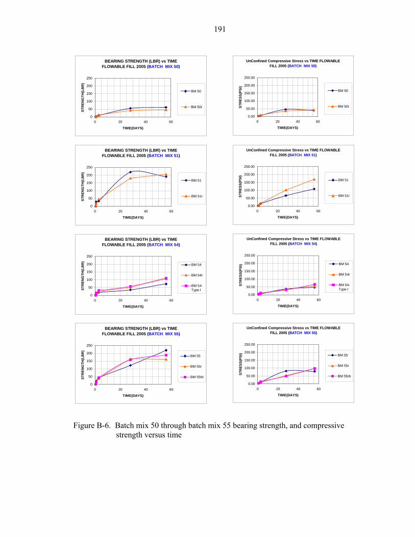
191
BEARING STRENGTH (LBR) vs TIME FLOWABLE FILL 2005 (BATCH MIX 50)
0
50
100
150
200
250
0 20 40 60
TIME(DAYS)
STR
ENG
TH(L
BR
)
BM 50
BM 50r
BEARING STRENGTH (LBR) vs TIME FLOWABLE FILL 2005 (BATCH MIX 51)
0
50
100
150
200
250
0 20 40 60
TIME(DAYS)
STR
ENG
TH(L
BR
)
BM 51
BM 51r
BEARING STRENGTH (LBR) vs TIME FLOWABLE FILL 2005 (BATCH MIX 54)
0
50
100
150
200
250
0 20 40 60
TIME(DAYS)
STR
ENG
TH(L
BR
)
BM 54
BM 54r
BM 54-Type I
BEARING STRENGTH (LBR) vs TIME FLOWABLE FILL 2005 (BATCH MIX 55)
0
50
100
150
200
250
0 20 40 60
TIME(DAYS)
STR
ENG
TH(L
BR
)
BM 55
BM 55r
BM 55rb
UnConfined Compressive Stress vs TIME FLOWABLE FILL 2005 (BATCH MIX 50)
0.00
50.00
100.00
150.00
200.00
250.00
0 20 40 60
TIME(DAYS)
STR
ESS(
PSI)
BM 50
BM 50r
UnConfined Compressive Stress vs TIME FLOWABLE FILL 2005 (BATCH MIX 54)
0.00
50.00
100.00
150.00
200.00
250.00
0 20 40 60
TIME(DAYS)
STR
ESS(
PSI) BM 54
BM 54r
BM 54-Type I
UnConfined Compressive Stress vs TIME FLOWABLE FILL 2005 (BATCH MIX 51)
0.00
50.00
100.00
150.00
200.00
250.00
0 20 40 60
TIME(DAYS)
STR
ESS(
PSI)
BM 51
BM 51r
UnConfined Compressive Stress vs TIME FLOWABLE FILL 2005 (BATCH MIX 55)
0.00
50.00
100.00
150.00
200.00
250.00
0 20 40 60
TIME(DAYS)
STR
ESS(
PSI) BM 55
BM 55r
BM 55rb
Figure B-6. Batch mix 50 through batch mix 55 bearing strength, and compressive strength versus time
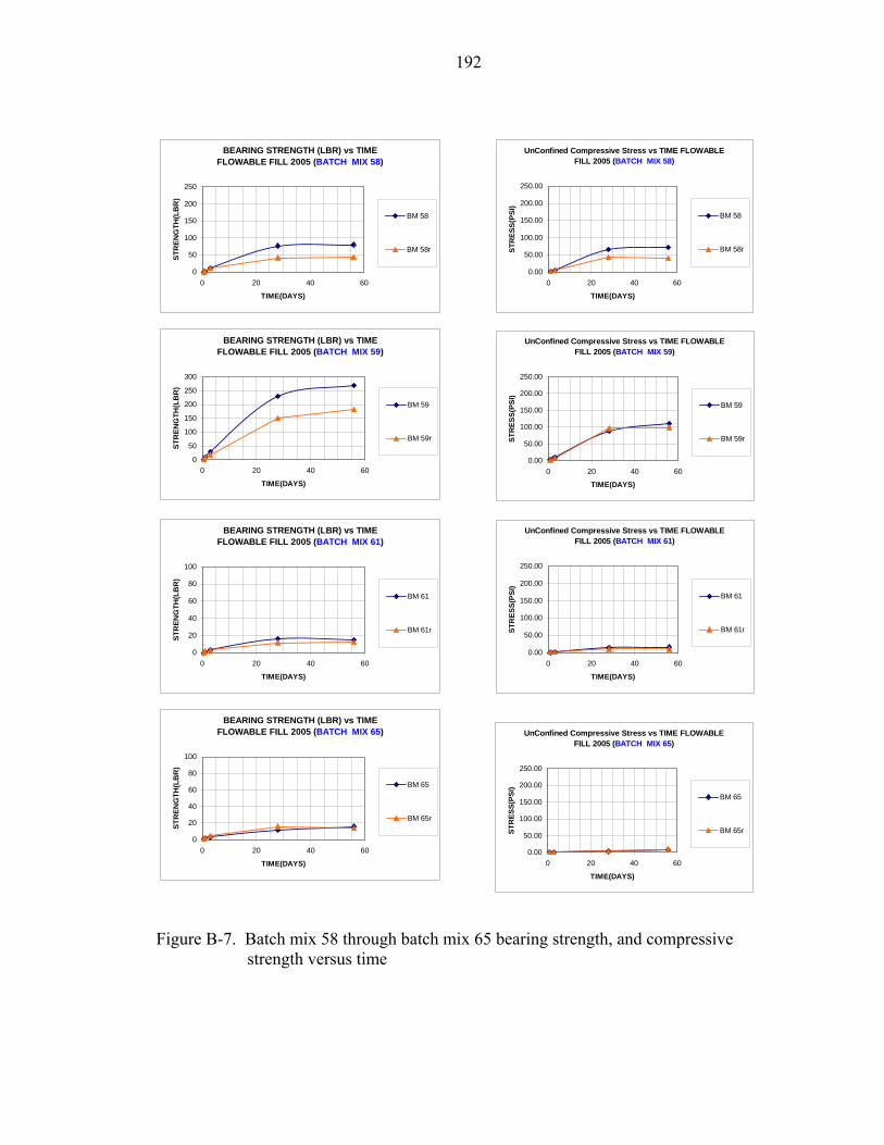
192
BEARING STRENGTH (LBR) vs TIME FLOWABLE FILL 2005 (BATCH MIX 58)
0
50
100
150
200
250
0 20 40 60
TIME(DAYS)
STR
ENG
TH(L
BR
)
BM 58
BM 58r
BEARING STRENGTH (LBR) vs TIME FLOWABLE FILL 2005 (BATCH MIX 59)
0
50
100
150
200
250
300
0 20 40 60
TIME(DAYS)
STR
ENG
TH(L
BR
)
BM 59
BM 59r
BEARING STRENGTH (LBR) vs TIME FLOWABLE FILL 2005 (BATCH MIX 61)
0
20
40
60
80
100
0 20 40 60
TIME(DAYS)
STR
ENG
TH(L
BR
)
BM 61
BM 61r
BEARING STRENGTH (LBR) vs TIME FLOWABLE FILL 2005 (BATCH MIX 65)
0
20
40
60
80
100
0 20 40 60
TIME(DAYS)
STR
ENG
TH(L
BR
)
BM 65
BM 65r
UnConfined Compressive Stress vs TIME FLOWABLE FILL 2005 (BATCH MIX 58)
0.00
50.00
100.00
150.00
200.00
250.00
0 20 40 60
TIME(DAYS)
STR
ESS(
PSI)
BM 58
BM 58r
UnConfined Compressive Stress vs TIME FLOWABLE FILL 2005 (BATCH MIX 61)
0.00
50.00
100.00
150.00
200.00
250.00
0 20 40 60
TIME(DAYS)
STR
ESS(
PSI)
BM 61
BM 61r
UnConfined Compressive Stress vs TIME FLOWABLE FILL 2005 (BATCH MIX 59)
0.00
50.00
100.00
150.00
200.00
250.00
0 20 40 60
TIME(DAYS)
STR
ESS(
PSI)
BM 59
BM 59r
UnConfined Compressive Stress vs TIME FLOWABLE FILL 2005 (BATCH MIX 65)
0.00
50.00
100.00
150.00
200.00
250.00
0 20 40 60
TIME(DAYS)
STR
ESS(
PSI)
BM 65
BM 65r
Figure B-7. Batch mix 58 through batch mix 65 bearing strength, and compressive strength versus time
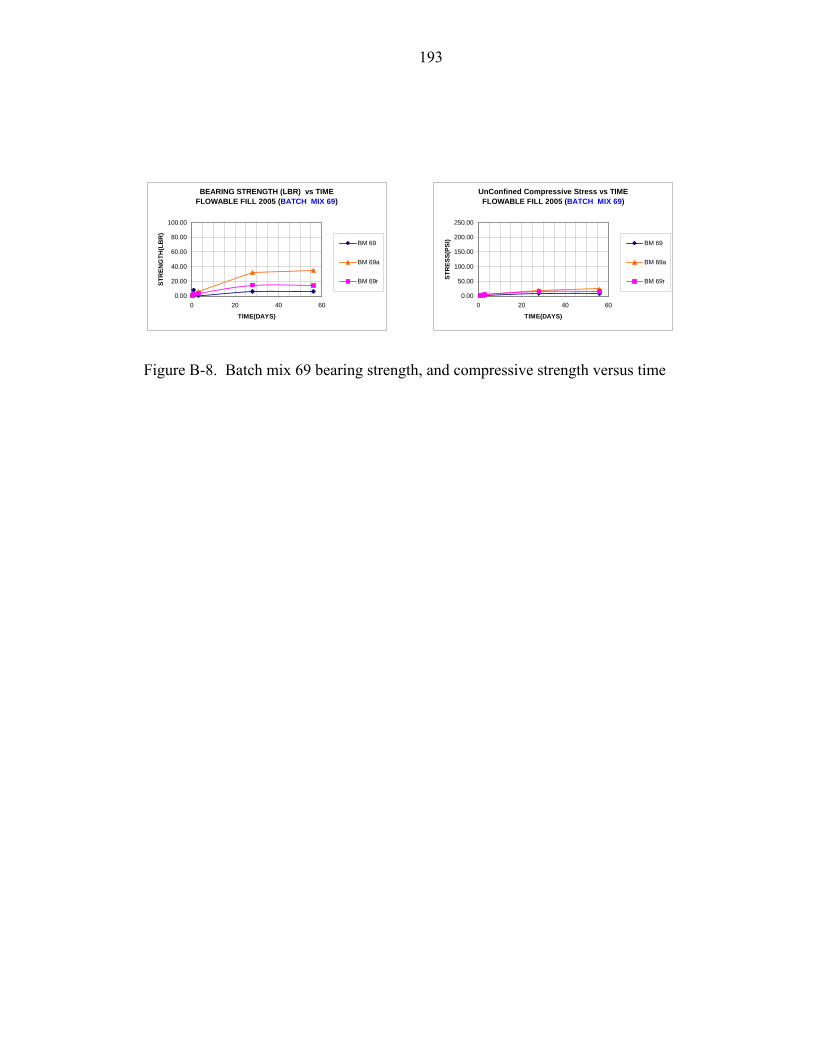
193
UnConfined Compressive Stress vs TIME FLOWABLE FILL 2005 (BATCH MIX 69)
0.00
50.00
100.00
150.00
200.00
250.00
0 20 40 60
TIME(DAYS)
STR
ESS(
PSI) BM 69
BM 69a
BM 69r
BEARING STRENGTH (LBR) vs TIME FLOWABLE FILL 2005 (BATCH MIX 69)
0.00
20.00
40.00
60.00
80.00
100.00
0 20 40 60
TIME(DAYS)
STR
ENG
TH(L
BR
)
BM 69
BM 69a
BM 69r
Figure B-8. Batch mix 69 bearing strength, and compressive strength versus time

194
Table B-1. Batch mix 4 through batch mix 22 proctor penetrometer resistance
BM#23 BM#33Time BM 23 BM 23r Time BM 33 BM 33r
psi psi psi psi6 hrs 50 23 6 hrs 18 171 day 135 113 1 day 47 382 day 2403 2600 2 day 177 --3 day 1133 900 3 day 67 6828 day 2600 2600 28 day 250 23756 day 2600 2600 56 day 217 417
BM#24 BM#34Time BM 24 BM 24r Time BM 34 BM 34r
psi psi psi psi6 hrs 28 -- 6 hrs 21 --1 day 170 120 1 day 77 1272 day 2600 2600 2 day 1000 15003 day 967 517 3 day 350 30028 day 2600 -- 28 day 2600 260056 day 2600 -- 56 day 2600 2600
BM#25 BM#40Time BM 25 BM 25-Type I BM 25r Time BM 40 BM 40r
psi psi psi psi psi6 hrs 35 16 14 6 hrs 6 01 day 83 53 49 1 day 147 6332 day 533 187 170 2 day -- 25333 day 140 90 102 3 day 1200 246728 day 1100 153 200 28 day 2600 260056 day -- -- 227 56 day 2600 2600
BM#26 BM#44Time BM 26 BM 26r Time BM 44 BM 44r
psi psi psi psi6 hrs 13 31 6 hrs 24 81 day 50 213 1 day 350 4552 day -- 1367 2 day 2600 26003 day 200 390 3 day 767 200028 day 2600 2600 28 day 2600 260056 day 2600 2600 56 day 2600 2600
BM#30 BM#48Time BM 30 BM 30r Time BM 48 BM 48-Type I BM 48r BM 48rb
psi psi psi psi psi psi6 hrs 23 20 6 hrs 0 9 13 231 day 70 290 1 day 167 287 420 3242 day 1400 700 2 day 2600 2600 2600 26003 day 267 -- 3 day 1900 1867 2600 125028 day 2133 683 28 day 2600 2600 2600 260056 day 2600 2567 56 day 2600 -- 2600 2600
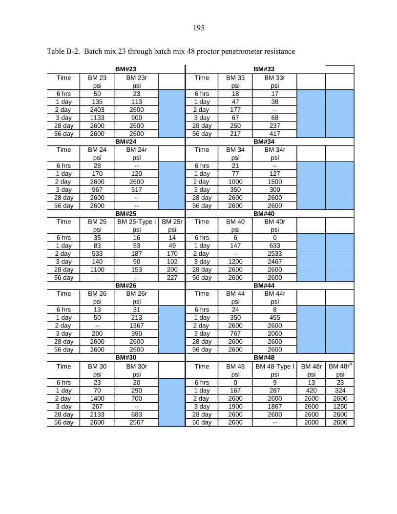
195
Table B-2. Batch mix 23 through batch mix 48 proctor penetrometer resistance
BM#23 BM#33Time BM 23 BM 23r Time BM 33 BM 33r
psi psi psi psi6 hrs 50 23 6 hrs 18 171 day 135 113 1 day 47 382 day 2403 2600 2 day 177 --3 day 1133 900 3 day 67 6828 day 2600 2600 28 day 250 23756 day 2600 2600 56 day 217 417
BM#24 BM#34Time BM 24 BM 24r Time BM 34 BM 34r
psi psi psi psi6 hrs 28 -- 6 hrs 21 --1 day 170 120 1 day 77 1272 day 2600 2600 2 day 1000 15003 day 967 517 3 day 350 30028 day 2600 -- 28 day 2600 260056 day 2600 -- 56 day 2600 2600
BM#25 BM#40Time BM 25 BM 25-Type I BM 25r Time BM 40 BM 40r
psi psi psi psi psi6 hrs 35 16 14 6 hrs 6 01 day 83 53 49 1 day 147 6332 day 533 187 170 2 day -- 25333 day 140 90 102 3 day 1200 246728 day 1100 153 200 28 day 2600 260056 day -- -- 227 56 day 2600 2600
BM#26 BM#44Time BM 26 BM 26r Time BM 44 BM 44r
psi psi psi psi6 hrs 13 31 6 hrs 24 81 day 50 213 1 day 350 4552 day -- 1367 2 day 2600 26003 day 200 390 3 day 767 200028 day 2600 2600 28 day 2600 260056 day 2600 2600 56 day 2600 2600
BM#30 BM#48Time BM 30 BM 30r Time BM 48 BM 48-Type I BM 48r BM 48rb
psi psi psi psi psi psi6 hrs 23 20 6 hrs 0 9 13 231 day 70 290 1 day 167 287 420 3242 day 1400 700 2 day 2600 2600 2600 26003 day 267 -- 3 day 1900 1867 2600 125028 day 2133 683 28 day 2600 2600 2600 260056 day 2600 2567 56 day 2600 -- 2600 2600

196
Table B-3. Batch mix 50 through batch mix 69 proctor penetrometer resistance
BM#50 BM#59
Time BM 50 BM 50r Time BM 59 BM 59rpsi psi psi psi
6 hrs 0 -- 6 hrs 25 01 day 95 -- 1 day 240 602 day 580 -- 2 day 2600 26003 day 233 -- 3 day 1533 28728 day 1967 -- 28 day 2600 260056 day 1667 -- 56 day 2600 2600
BM#51 BM#61Time BM 51 BM 51r Time BM 61 BM 61r
psi psi psi psi6 hrs 15 19 6 hrs 0 01 day 227 180 1 day 0 332 day 2600 2600 2 day 93 553 day 1167 700 3 day 64 5428 day 2600 -- 28 day 170 16056 day 2600 -- 56 day 120 110
BM#54 BM#65Time BM 54 BM 54-Type I BM 54r Time BM 65 BM 65r
psi psi psi psi psi6 hrs 2 17 12 6 hrs 2 01 day 110 153 153 1 day 32 352 day 667 1433 550 2 day 110 1073 day 330 517 457 3 day 40 5328 day 1300 1400 1600 28 day 150 16356 day 1700 2600 2600 56 day 407 153
BM#55 BM#69Time BM 55 BM 55r BM 55rb Time BM 69 BM 69a BM 69r
psi psi psi psi psi psi6 hrs 22 22 10 6 hrs 0 8 01 day 333 202 257 1 day 10 27 302 day 2267 2400 2600 2 day 60 407 1573 day 1300 550 425 3 day 25 113 6428 day 2600 2600 2600 28 day 93 677 19056 day 2600 2600 2600 56 day 90 343 115
BM#58Time BM 58 BM 58r
psi psi6 hrs 3 01 day 64 612 day 1200 10753 day 110 17728 day 1833 88356 day 2200 825

197
Table B-4. Batch mix 4 through batch mix 22 individual 2-days oven LBR strength
BM#4 BM#16
Sample No. BM 4 BM 4a BM 4r Sample No. BM 16 BM 16a BM 16r(LBR) (LBR) (LBR) (LBR) (LBR) (LBR)
1 29 110 160 1 119 99 1502 34 92 167 2 104 141 1173 35 102 195 3 107 83 112
BM#8 BM#18Sample No. BM 8 BM 8r Sample No. BM 18 BM 18r
(LBR) (LBR) (LBR) (LBR)1 65 37 1 30 232 60 32 2 50 263 129 35 3 31 19
BM#12 BM#19Sample No. BM 12 BM 12r Sample No. BM 19 BM 19r
(LBR) (LBR) (LBR) (LBR)1 160 202 1 51 672 137 185 2 66 983 138 203 3 69 152
BM#14 BM#20Sample No. BM 14 BM 14r Sample No. BM 20 BM 20r
(LBR) (LBR) (LBR) (LBR)1 69 33 1 103 962 47 31 2 71 1213 66 32 3 87 107
BM#15 BM#22Sample No. BM 15 BM 15-Type I BM 15r Sample No. BM 22 BM 22r
(LBR) (LBR) (LBR) (LBR) (LBR)1 75 146 136 1 34 402 63 126 87 2 36 493 60 164 99 3 41 50
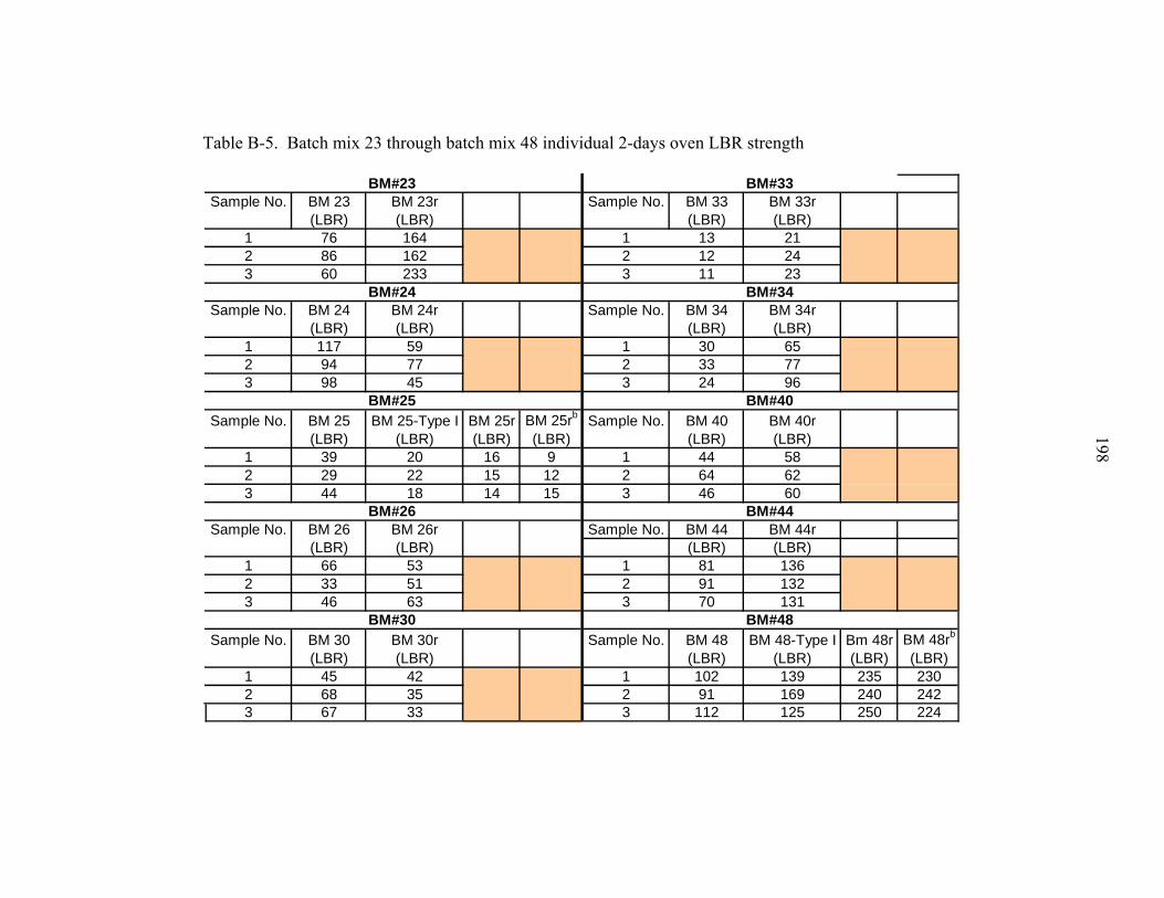
198
Table B-5. Batch mix 23 through batch mix 48 individual 2-days oven LBR strength
BM#23 BM#33Sample No. BM 23 BM 23r Sample No. BM 33 BM 33r
(LBR) (LBR) (LBR) (LBR)1 76 164 1 13 212 86 162 2 12 243 60 233 3 11 23
BM#24 BM#34Sample No. BM 24 BM 24r Sample No. BM 34 BM 34r
(LBR) (LBR) (LBR) (LBR)1 117 59 1 30 652 94 77 2 33 773 98 45 3 24 96
BM#25 BM#40Sample No. BM 25 BM 25-Type I BM 25r BM 25rb Sample No. BM 40 BM 40r
(LBR) (LBR) (LBR) (LBR) (LBR) (LBR)1 39 20 16 9 1 44 582 29 22 15 12 2 64 623 44 18 14 15 3 46 60
BM#26 BM#44Sample No. BM 26 BM 26r Sample No. BM 44 BM 44r
(LBR) (LBR) (LBR) (LBR)1 66 53 1 81 1362 33 51 2 91 1323 46 63 3 70 131
BM#30 BM#48Sample No. BM 30 BM 30r Sample No. BM 48 BM 48-Type I Bm 48r BM 48rb
(LBR) (LBR) (LBR) (LBR) (LBR) (LBR)1 45 42 1 102 139 235 2302 68 35 2 91 169 240 2423 67 33 3 112 125 250 224

199
Table B-6. Batch mix 50 through batch mix 69 individual 2-days oven LBR strength
BM#50 BM#59
Sample No. BM 50 BM 50r Sample No. BM 59 BM 59r(LBR) (LBR) (LBR) (LBR)
1 21 44 1 71 1352 19 49 2 96 1093 19 43 3 78 164
BM#51 BM#61Sample No. BM 51 BM 51r Sample No. BM 61 BM 61r
(LBR) (LBR) (LBR) (LBR)1 88 71 1 8 42 81 106 2 6 53 98 106 3 6 4
BM#54 BM#65Sample No. BM 54 BM 54-Type I BM 54r Sample No. BM 65 BM 65r
(LBR) (LBR) (LBR) (LBR) (LBR)1 37 54 49 1 8 112 28 49 43 2 10 133 33 68 42 3 9 8
BM#55 BM#69Sample No. BM 55 BM 55r BM 55rb Sample No. BM 69 BM 69a BM 69r
(LBR) (LBR) (LBR) (LBR) (LBR) (LBR)1 56 74 117 1 1 33 92 52 108 119 2 1 22 103 79 98 152 3 1 8 11
BM#58Sample No. BM 58 BM 58r
(LBR) (LBR)1 42 722 47 603 37 70

200
APPENDIX C ANALYSIS OF VARIANCE (ANOVA), PARAMETERS, AND
STANDARD ERROR FOR MODELS
This appendix contains the analysis of variances (ANOVA), parameters and
standard error for the models.

201
Table C-1. Analysis of variance (ANOVA) for 28-day_LBR Dependent Variable: y Sum of Source DF Squares Mean Square F Value Pr > F Model 14 862512.761 61608.054 62.45 <.0001 Error 159 156865.944 986.578 Corrected Total 173 1019378.705 R-Square Coeff Var Root MSE y Mean 0.846116 27.71796 31.40984 113.3195 Source DF Type I SS Mean Square F Value Pr > F a 1 651259.1367 651259.1367 660.12 <.0001 b 1 70256.1787 70256.1787 71.21 <.0001 c 1 2652.3252 2652.3252 2.69 0.1031 d 1 1876.9757 1876.9757 1.90 0.1697 a*a 1 7236.2518 7236.2518 7.33 0.0075 c*c 1 4061.4278 4061.4278 4.12 0.0441 d*d 1 78089.4362 78089.4362 79.15 <.0001 a*b 1 12646.5644 12646.5644 12.82 0.0005 a*c 1 25540.2951 25540.2951 25.89 <.0001 a*d 1 466.9930 466.9930 0.47 0.4925 b*c 1 15.7662 15.7662 0.02 0.8996 b*d 1 6183.1408 6183.1408 6.27 0.0133 c*d 1 770.7810 770.7810 0.78 0.3781
Table C-2. Parameters and standard error for 28-day_LBR Dependent Variable: y Standard Parameter Estimate Error t Value Pr > |t| Intercept 299.0395348 549.8721856 0.55 0.5850 a 0.9275712 3.7396744 0.25 0.8044 b -18.7800976 12.5361909 -1.50 0.1361 c -24.8168169 111.9847756 -0.22 0.8249 d -3.2137849 1.8474553 -1.74 0.0839 a*a -0.0007561 0.0063013 -0.12 0.9046 c*c 1.1867884 5.1651063 0.23 0.8186 d*d 0.0791980 0.0091503 8.66 <.0001 a*b 0.0337116 0.0523819 0.64 0.5208 a*c -0.1446410 0.3919195 -0.37 0.7126 a*d -0.0042579 0.0065837 -0.65 0.5187 b*c 1.1495852 1.3251259 0.87 0.3870 b*d 0.0303699 0.0277731 1.09 0.2758 c*d -0.1140068 0.1289825 -0.88 0.3781

202
Table C-3. Analysis of variance (ANOVA) for 28-day_ psi Dependent Variable: y Sum of Source DF Squares Mean Square F Value Pr > F Model 14 296002.7645 21143.0546 83.50 <.0001 Error 159 40262.4392 253.2229 Corrected Total 173 336265.2037 R-Square Coeff Var Root MSE y Mean 0.880266 25.76665 15.91298 61.75805 Source DF Type I SS Mean Square F Value Pr > F a 1 242503.7096 242503.7096 957.67 <.0001 b 1 24517.8816 24517.8816 96.82 <.0001 c 1 636.4043 636.4043 2.51 0.1149 d 1 1380.3527 1380.3527 5.45 0.0208 a*a 1 0.0386 0.0386 0.00 0.9902 c*c 1 8535.1258 8535.1258 33.71 <.0001 d*d 1 10721.9032 10721.9032 42.34 <.0001 a*b 1 1984.1722 1984.1722 7.84 0.0058 a*c 1 2513.1280 2513.1280 9.92 0.0019 a*d 1 862.3962 862.3962 3.41 0.0668 b*c 1 13.4709 13.4709 0.05 0.8179 b*d 1 983.6902 983.6902 3.88 0.0505 c*d 1 1249.2885 1249.2885 4.93 0.0278
Table C-4. Parameters and standard error for 28-day_psi Dependent Variable: y Standard Parameter Estimate Error t Value Pr > |t| Intercept 94.93413075 278.5784124 0.34 0.7324 a 1.52314981 1.8946086 0.80 0.4226 b -0.68144093 6.3511344 -0.11 0.9147 c -45.61558093 56.7341681 -0.80 0.4226 d 1.23005865 0.9359651 1.31 0.1907 a*a -0.00293926 0.0031924 -0.92 0.3586 c*c 3.36478471 2.6167665 1.29 0.2004 d*d 0.02723015 0.0046358 5.87 <.0001 a*b -0.00963500 0.0265379 -0.36 0.7170 a*c -0.06353336 0.1985558 -0.32 0.7494 a*d -0.01002679 0.0033354 -3.01 0.0031 b*c 0.23249384 0.6713405 0.35 0.7296 b*d -0.04175278 0.0140705 -2.97 0.0035 c*d -0.14514315 0.0653456 -2.22 0.0278
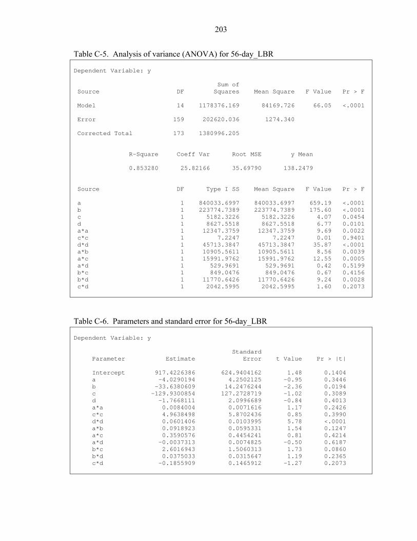
203
Table C-5. Analysis of variance (ANOVA) for 56-day_LBR Dependent Variable: y Sum of Source DF Squares Mean Square F Value Pr > F Model 14 1178376.169 84169.726 66.05 <.0001 Error 159 202620.036 1274.340 Corrected Total 173 1380996.205 R-Square Coeff Var Root MSE y Mean 0.853280 25.82166 35.69790 138.2479 Source DF Type I SS Mean Square F Value Pr > F a 1 840033.6997 840033.6997 659.19 <.0001 b 1 223774.7389 223774.7389 175.60 <.0001 c 1 5182.3226 5182.3226 4.07 0.0454 d 1 8627.5518 8627.5518 6.77 0.0101 a*a 1 12347.3759 12347.3759 9.69 0.0022 c*c 1 7.2247 7.2247 0.01 0.9401 d*d 1 45713.3847 45713.3847 35.87 <.0001 a*b 1 10905.5611 10905.5611 8.56 0.0039 a*c 1 15991.9762 15991.9762 12.55 0.0005 a*d 1 529.9691 529.9691 0.42 0.5199 b*c 1 849.0476 849.0476 0.67 0.4156 b*d 1 11770.6426 11770.6426 9.24 0.0028 c*d 1 2042.5995 2042.5995 1.60 0.2073
Table C-6. Parameters and standard error for 56-day_LBR Dependent Variable: y Standard Parameter Estimate Error t Value Pr > |t| Intercept 917.4226386 624.9404162 1.48 0.1404 a -4.0290194 4.2502125 -0.95 0.3446 b -33.6380609 14.2476244 -2.36 0.0194 c -129.9300854 127.2728719 -1.02 0.3089 d -1.7668111 2.0996689 -0.84 0.4013 a*a 0.0084004 0.0071616 1.17 0.2426 c*c 4.9638498 5.8702436 0.85 0.3990 d*d 0.0601406 0.0103995 5.78 <.0001 a*b 0.0918923 0.0595331 1.54 0.1247 a*c 0.3590576 0.4454241 0.81 0.4214 a*d -0.0037313 0.0074825 -0.50 0.6187 b*c 2.6016943 1.5060313 1.73 0.0860 b*d 0.0375033 0.0315647 1.19 0.2365 c*d -0.1855909 0.1465912 -1.27 0.2073

204
Table C-7. Analysis of variance (ANOVA) for 56-day_psi Dependent Variable: y Sum of Source DF Squares Mean Square F Value Pr > F Model 14 366547.1182 26181.9370 68.94 <.0001 Error 159 60385.4411 379.7826 Corrected Total 173 426932.5593 R-Square Coeff Var Root MSE y Mean 0.858560 24.21001 19.48801 80.49569 Source DF Type I SS Mean Square F Value Pr > F a 1 335819.4915 335819.4915 884.24 <.0001 b 1 2795.4529 2795.4529 7.36 0.0074 c 1 2995.0574 2995.0574 7.89 0.0056 d 1 9.3865 9.3865 0.02 0.8753 a*a 1 138.2629 138.2629 0.36 0.5471 c*c 1 1787.7336 1787.7336 4.71 0.0315 d*d 1 9314.4984 9314.4984 24.53 <.0001 a*b 1 496.2811 496.2811 1.31 0.2547 a*c 1 11854.8823 11854.8823 31.21 <.0001 a*d 1 42.2716 42.2716 0.11 0.7391 b*c 1 988.1203 988.1203 2.60 0.1087 b*d 1 89.4557 89.4557 0.24 0.6281 c*d 1 6.2337 6.2337 0.02 0.8982
Table C-8. Parameters and standard error for 56-day_psi Dependent Variable: y Standard Parameter Estimate Error t Value Pr > |t| Intercept 152.8311117 341.1642685 0.46 0.6453 a -0.2440199 2.3202542 -0.11 0.9164 b -14.1298028 7.7779901 -1.82 0.0712 c -1.5069197 69.4801538 -0.02 0.9827 d -1.4146273 1.1462405 -1.23 0.2190 a*a 0.0013497 0.0039096 0.35 0.7304 c*c -1.2148056 3.2046533 -0.38 0.7051 d*d 0.0289481 0.0056773 5.10 <.0001 a*b 0.0527250 0.0325000 1.62 0.1067 a*c 0.0130316 0.2431637 0.05 0.9573 a*d -0.0005653 0.0040848 -0.14 0.8901 b*c 1.1438790 0.8221649 1.39 0.1661 b*d -0.0041910 0.0172316 -0.24 0.8082 c*d 0.0102527 0.0800263 0.13 0.8982

205
Table C-9. Analysis of variance (ANOVA) for percent volume change Dependent Variable: y Sum of Source DF Squares Mean Square F Value Pr > F Model 14 95.1002556 6.7928754 15.26 <.0001 Error 159 70.7689599 0.4450878 Corrected Total 173 165.8692155 R-Square Coeff Var Root MSE y Mean 0.573345 62.39830 0.667149 1.069178 Source DF Type I SS Mean Square F Value Pr > F a 1 0.66668565 0.66668565 1.50 0.2228 b 1 23.28073600 23.28073600 52.31 <.0001 c 1 20.21083693 20.21083693 45.41 <.0001 d 1 20.97958837 20.97958837 47.14 <.0001 a*a 1 1.19723827 1.19723827 2.69 0.1030 c*c 1 19.71027092 19.71027092 44.28 <.0001 d*d 1 0.07402647 0.07402647 0.17 0.6840 a*b 1 0.74268437 0.74268437 1.67 0.1983 a*c 1 3.73650570 3.73650570 8.39 0.0043 a*d 1 2.48076185 2.48076185 5.57 0.0194 b*c 1 0.02362357 0.02362357 0.05 0.8181 b*d 1 0.74311573 0.74311573 1.67 0.1982 c*d 1 1.17469349 1.17469349 2.64 0.1062
Table C-10. Parameters and standard error for percent volume change Dependent Variable: y Standard Parameter Estimate Error t Value Pr > |t| Intercept -3.945266055 11.67935406 -0.35 0.7248 a -0.004565043 0.07943115 -0.06 0.9542 b 0.193485690 0.26627026 0.73 0.4685 c -0.667434645 2.37857065 -0.28 0.7794 d 0.028359595 0.03924018 0.72 0.4709 a*a 0.000010491 0.00013384 0.08 0.9376 c*c 0.037335267 0.10970750 0.34 0.7341 d*d -0.000184863 0.00019435 -0.95 0.3430 a*b -0.000115511 0.00111260 -0.10 0.9174 a*c 0.009037169 0.00832442 1.09 0.2793 a*d -0.000070018 0.00013984 -0.50 0.6173 b*c 0.012815636 0.02814584 0.46 0.6495 b*d -0.000164766 0.00058990 -0.28 0.7804 c*d -0.004450691 0.00273961 -1.62 0.1062
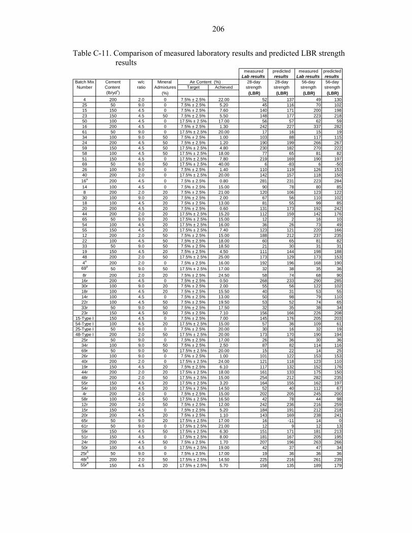
206
Table C-11. Comparison of measured laboratory results and predicted LBR strength results
measured predicted measured predictedLab results results Lab results results
Batch Mix Cement w/c Mineral Air Content (%) 28-day 28-day 56-day 56-dayNumber Content ratio Admixtures Target Achieved strength strength strength strength
(lb/yd3) (%) (LBR) (LBR) (LBR) (LBR)4 200 2.0 0 7.5% ± 2.5% 22.00 52 137 49 130
25 50 9.0 0 7.5% ± 2.5% 5.20 45 116 70 10215 150 4.5 0 7.5% ± 2.5% 7.60 140 171 200 19823 150 4.5 50 7.5% ± 2.5% 5.50 148 177 223 21850 100 4.5 0 17.5% ± 2.5% 17.00 56 57 62 5916 200 4.5 0 7.5% ± 2.5% 1.30 242 227 337 28261 50 9.0 0 17.5% ± 2.5% 20.00 17 16 15 1934 100 9.0 50 7.5% ± 2.5% 1.00 103 88 117 11524 200 4.5 50 7.5% ± 2.5% 1.20 190 199 266 26759 150 4.5 50 17.5% ± 2.5% 4.80 230 182 270 22258 100 4.5 50 17.5% ± 2.5% 18.00 77 65 81 8251 150 4.5 0 17.5% ± 2.5% 7.80 219 169 190 19769 50 9.0 50 17.5% ± 2.5% 40.00 6 -83 6 -5026 100 9.0 0 7.5% ± 2.5% 1.40 110 119 126 15340 200 2.0 0 17.5% ± 2.5% 20.00 142 157 118 15016a 200 4.5 0 7.5% ± 2.5% 0.80 281 231 223 28414 100 4.5 0 7.5% ± 2.5% 15.00 90 78 80 858 200 2.0 20 7.5% ± 2.5% 21.00 120 106 123 122
30 100 9.0 20 7.5% ± 2.5% 2.00 67 56 110 10218 100 4.5 20 7.5% ± 2.5% 13.00 81 55 99 8520 200 4.5 20 7.5% ± 2.5% 0.60 131 173 192 24244 200 2.0 20 17.5% ± 2.5% 15.20 112 159 142 17665 50 9.0 20 17.5% ± 2.5% 15.00 12 2 16 1054 100 4.5 20 17.5% ± 2.5% 16.00 36 26 73 4955 150 4.5 20 17.5% ± 2.5% 7.40 123 121 220 16612 200 2.0 50 7.5% ± 2.5% 15.00 188 212 237 23522 100 4.5 50 7.5% ± 2.5% 18.00 60 65 81 8233 50 9.0 50 7.5% ± 2.5% 18.50 21 30 31 3119 150 4.5 20 7.5% ± 2.5% 4.50 111 144 198 18848 200 2.0 50 17.5% ± 2.5% 25.00 173 129 173 1534a 200 2.0 0 7.5% ± 2.5% 16.00 192 196 168 190
69a 50 9.0 50 17.5% ± 2.5% 17.00 32 38 35 368r 200 2.0 20 7.5% ± 2.5% 24.50 58 74 68 90
16r 200 4.5 0 7.5% ± 2.5% 0.50 268 233 290 28530r 100 9.0 20 7.5% ± 2.5% 2.00 55 56 122 10218r 100 4.5 20 7.5% ± 2.5% 15.50 40 31 53 5514r 100 4.5 0 7.5% ± 2.5% 13.00 50 98 79 11022r 100 4.5 50 7.5% ± 2.5% 19.50 53 52 74 6533r 50 9.0 50 7.5% ± 2.5% 17.50 32 35 38 3423r 150 4.5 50 7.5% ± 2.5% 7.10 156 166 226 208
15-Type I 150 4.5 0 7.5% ± 2.5% 7.00 145 176 205 20354-Type I 100 4.5 20 17.5% ± 2.5% 15.00 57 36 109 6125-Type I 50 9.0 0 7.5% ± 2.5% 20.00 30 16 32 1948-Type I 200 2.0 50 17.5% ± 2.5% 20.00 173 170 190 194
25r 50 9.0 0 7.5% ± 2.5% 17.00 26 36 30 3634r 100 9.0 50 7.5% ± 2.5% 2.50 87 82 114 11669r 50 9.0 50 17.5% ± 2.5% 20.00 15 22 14 2526r 100 9.0 0 7.5% ± 2.5% 1.00 101 122 153 15340r 200 2.0 0 17.5% ± 2.5% 24.00 121 118 123 11019r 150 4.5 20 7.5% ± 2.5% 6.10 117 132 152 17644r 200 2.0 20 17.5% ± 2.5% 18.00 161 133 175 15048r 200 2.0 50 17.5% ± 2.5% 15.00 254 212 282 23555r 150 4.5 20 17.5% ± 2.5% 3.20 164 155 162 19754r 100 4.5 20 17.5% ± 2.5% 14.50 52 40 112 674r 200 2.0 0 7.5% ± 2.5% 15.00 202 205 245 200
58r 100 4.5 50 17.5% ± 2.5% 16.50 42 78 44 9812r 200 2.0 50 7.5% ± 2.5% 12.00 242 236 216 25915r 150 4.5 0 7.5% ± 2.5% 5.20 184 191 212 21820r 200 4.5 20 7.5% ± 2.5% 1.10 143 169 238 24165r 50 9.0 20 17.5% ± 2.5% 17.00 16 -11 14 061r 50 9.0 0 17.5% ± 2.5% 21.00 12 9 12 1359r 150 4.5 50 17.5% ± 2.5% 6.30 151 171 181 21351r 150 4.5 0 17.5% ± 2.5% 8.00 181 167 205 19524r 200 4.5 50 7.5% ± 2.5% 1.70 207 196 263 26650r 100 4.5 0 17.5% ± 2.5% 19.00 42 37 47 3425rb 50 9.0 0 7.5% ± 2.5% 17.00 19 36 36 3648rb 200 2.0 50 17.5% ± 2.5% 14.50 225 216 261 23955rb 150 4.5 20 17.5% ± 2.5% 5.70 158 135 189 179

207
Table C-12. Comparison of measured laboratory results and predicted compressive
strength results measured predicted measured predicted
Lab results results Lab results resultsBatch Mix Cement w/c Mineral Air Content (%) 28-day 28-day 56-day 56-dayNumber Content ratio Admixtures Target Achieved strength strength strength strength
(lb/yd3) (%) (psi) (psi) (psi) (psi)4 200 2.0 0 7.5% ± 2.5% 22.00 50 132 41 127
25 50 9.0 0 7.5% ± 2.5% 5.20 17 2 29 3215 150 4.5 0 7.5% ± 2.5% 7.60 58 69 93 11623 150 4.5 50 7.5% ± 2.5% 5.50 79 82 124 11750 100 4.5 0 17.5% ± 2.5% 17.00 45 42 39 5316 200 4.5 0 7.5% ± 2.5% 1.30 89 86 133 14061 50 9.0 0 17.5% ± 2.5% 20.00 14 16 17 1434 100 9.0 50 7.5% ± 2.5% 1.00 30 35 44 4624 200 4.5 50 7.5% ± 2.5% 1.20 79 80 155 13859 150 4.5 50 17.5% ± 2.5% 4.80 89 84 111 11758 100 4.5 50 17.5% ± 2.5% 18.00 66 51 72 4751 150 4.5 0 17.5% ± 2.5% 7.80 67 69 108 11669 50 9.0 50 17.5% ± 2.5% 40.00 9 -10 8 -1426 100 9.0 0 7.5% ± 2.5% 1.40 22 23 34 4440 200 2.0 0 17.5% ± 2.5% 20.00 138 136 114 12916a 200 4.5 0 7.5% ± 2.5% 0.80 70 86 148 14014 100 4.5 0 7.5% ± 2.5% 15.00 58 43 69 618 200 2.0 20 7.5% ± 2.5% 21.00 100 106 129 108
30 100 9.0 20 7.5% ± 2.5% 2.00 14 11 34 2818 100 4.5 20 7.5% ± 2.5% 13.00 33 36 43 5020 200 4.5 20 7.5% ± 2.5% 0.60 86 69 132 12144 200 2.0 20 17.5% ± 2.5% 15.20 107 123 114 11665 50 9.0 20 17.5% ± 2.5% 15.00 4 -2 8 354 100 4.5 20 17.5% ± 2.5% 16.00 39 32 46 3955 150 4.5 20 17.5% ± 2.5% 7.40 81 55 81 9812 200 2.0 50 7.5% ± 2.5% 15.00 143 130 139 13022 100 4.5 50 7.5% ± 2.5% 18.00 42 51 37 4733 50 9.0 50 7.5% ± 2.5% 18.50 13 15 15 1719 150 4.5 20 7.5% ± 2.5% 4.50 56 61 132 10148 200 2.0 50 17.5% ± 2.5% 25.00 109 88 135 1144a 200 2.0 0 7.5% ± 2.5% 16.00 115 144 105 135
69a 50 9.0 50 17.5% ± 2.5% 17.00 19 17 24 198r 200 2.0 20 7.5% ± 2.5% 24.50 63 95 57 103
16r 200 4.5 0 7.5% ± 2.5% 0.50 64 87 132 13930r 100 9.0 20 7.5% ± 2.5% 2.00 18 11 38 2818r 100 4.5 20 7.5% ± 2.5% 15.50 35 32 37 4114r 100 4.5 0 7.5% ± 2.5% 13.00 40 44 65 6822r 100 4.5 50 7.5% ± 2.5% 19.50 38 47 51 4133r 50 9.0 50 7.5% ± 2.5% 17.50 15 16 18 1823r 150 4.5 50 7.5% ± 2.5% 7.10 74 77 127 114
15-Type I 150 4.5 0 7.5% ± 2.5% 7.00 62 70 101 11654-Type I 100 4.5 20 17.5% ± 2.5% 15.00 33 33 67 4325-Type I 50 9.0 0 7.5% ± 2.5% 20.00 15 16 16 1448-Type I 200 2.0 50 17.5% ± 2.5% 20.00 143 109 139 122
25r 50 9.0 0 7.5% ± 2.5% 17.00 8 13 15 1734r 100 9.0 50 7.5% ± 2.5% 2.50 31 33 51 4869r 50 9.0 50 17.5% ± 2.5% 20.00 15 13 15 1426r 100 9.0 0 7.5% ± 2.5% 1.00 21 23 47 4340r 200 2.0 0 17.5% ± 2.5% 24.00 151 127 131 12419r 150 4.5 20 7.5% ± 2.5% 6.10 40 58 129 9944r 200 2.0 20 17.5% ± 2.5% 18.00 139 115 131 11248r 200 2.0 50 17.5% ± 2.5% 15.00 162 130 162 13055r 150 4.5 20 17.5% ± 2.5% 3.20 53 64 98 10354r 100 4.5 20 17.5% ± 2.5% 14.50 33 34 56 444r 200 2.0 0 7.5% ± 2.5% 15.00 159 147 161 136
58r 100 4.5 50 17.5% ± 2.5% 16.50 43 55 41 5312r 200 2.0 50 7.5% ± 2.5% 12.00 137 143 143 13415r 150 4.5 0 7.5% ± 2.5% 5.20 66 72 136 11820r 200 4.5 20 7.5% ± 2.5% 1.10 92 67 129 12265r 50 9.0 20 17.5% ± 2.5% 17.00 5 -2 24 161r 50 9.0 0 17.5% ± 2.5% 21.00 10 17 11 1359r 150 4.5 50 17.5% ± 2.5% 6.30 97 79 99 11551r 150 4.5 0 17.5% ± 2.5% 8.00 102 69 170 11524r 200 4.5 50 7.5% ± 2.5% 1.70 57 78 125 13950r 100 4.5 0 17.5% ± 2.5% 19.00 36 41 44 4625rb 50 9.0 0 7.5% ± 2.5% 17.00 7 13 16 1748rb 200 2.0 50 17.5% ± 2.5% 14.50 131 132 119 13055rb 150 4.5 20 17.5% ± 2.5% 5.70 49 59 100 100

208
Table C-13. Comparison of measured laboratory results and predicted percent volume change results
measured predictedLab results results
Batch Mix Cement w/c Mineral Air Content (%) Volume Volume Number Content ratio Admixtures Target Achieved change change
(lb/yd3) (%) (%) (%)4 200 2.0 0 7.5% ± 2.5% 22.00 0.14 2.2925 50 9.0 0 7.5% ± 2.5% 5.20 0.14 -1.4915 150 4.5 0 7.5% ± 2.5% 7.60 0.60 1.2323 150 4.5 50 7.5% ± 2.5% 5.50 0.19 0.1350 100 4.5 0 17.5% ± 2.5% 17.00 2.86 1.5916 200 4.5 0 7.5% ± 2.5% 1.30 2.10 1.7561 50 9.0 0 17.5% ± 2.5% 20.00 2.89 2.9934 100 9.0 50 7.5% ± 2.5% 1.00 0.26 -0.2524 200 4.5 50 7.5% ± 2.5% 1.20 0.31 0.9759 150 4.5 50 17.5% ± 2.5% 4.80 0.79 -0.0358 100 4.5 50 17.5% ± 2.5% 18.00 1.41 1.2851 150 4.5 0 17.5% ± 2.5% 7.80 0.98 1.2869 50 9.0 50 17.5% ± 2.5% 40.00 1.82 7.4926 100 9.0 0 7.5% ± 2.5% 1.40 1.66 1.2740 200 2.0 0 17.5% ± 2.5% 20.00 2.12 1.9016* 200 4.5 0 7.5% ± 2.5% 0.80 2.10 1.6314 100 4.5 0 7.5% ± 2.5% 15.00 0.35 1.118 200 2.0 20 7.5% ± 2.5% 21.00 3.11 2.0630 100 9.0 20 7.5% ± 2.5% 2.00 0.16 1.0018 100 4.5 20 7.5% ± 2.5% 13.00 0.57 0.5420 200 4.5 20 7.5% ± 2.5% 0.60 1.38 1.4044 200 2.0 20 17.5% ± 2.5% 15.20 1.33 0.9565 50 9.0 20 17.5% ± 2.5% 15.00 1.39 1.0554 100 4.5 20 17.5% ± 2.5% 16.00 0.52 1.2555 150 4.5 20 17.5% ± 2.5% 7.40 1.06 1.0512 200 2.0 50 7.5% ± 2.5% 15.00 0.29 0.6122 100 4.5 50 7.5% ± 2.5% 18.00 0.54 1.2833 50 9.0 50 7.5% ± 2.5% 18.50 0.46 1.1619 150 4.5 20 7.5% ± 2.5% 4.50 0.38 0.3848 200 2.0 50 17.5% ± 2.5% 25.00 0.54 2.484* 200 2.0 0 7.5% ± 2.5% 16.00 0.14 1.1269* 50 9.0 50 17.5% ± 2.5% 17.00 1.82 0.728r 200 2.0 20 7.5% ± 2.5% 24.50 3.11 2.7316r 200 4.5 0 7.5% ± 2.5% 0.50 2.10 1.5630r 100 9.0 20 7.5% ± 2.5% 2.00 0.16 1.0018r 100 4.5 20 7.5% ± 2.5% 15.50 0.57 1.1314r 100 4.5 0 7.5% ± 2.5% 13.00 0.35 0.6322r 100 4.5 50 7.5% ± 2.5% 19.50 0.54 1.6333r 50 9.0 50 7.5% ± 2.5% 17.50 0.46 0.8723r 150 4.5 50 7.5% ± 2.5% 7.10 0.19 0.49
15-Type I 150 4.5 0 7.5% ± 2.5% 7.00 0.31 1.0954-Type I 100 4.5 20 17.5% ± 2.5% 15.00 0.25 1.0125-Type I 50 9.0 0 7.5% ± 2.5% 20.00 0.89 2.9948-Type I 200 2.0 50 17.5% ± 2.5% 20.00 1.26 1.55
25r 50 9.0 0 7.5% ± 2.5% 17.00 0.41 2.0834r 100 9.0 50 7.5% ± 2.5% 2.50 0.26 0.1869r 50 9.0 50 17.5% ± 2.5% 20.00 1.82 1.6026r 100 9.0 0 7.5% ± 2.5% 1.00 1.66 1.1540r 200 2.0 0 17.5% ± 2.5% 24.00 2.12 2.6819r 150 4.5 20 7.5% ± 2.5% 6.10 0.38 0.7544r 200 2.0 20 17.5% ± 2.5% 18.00 1.33 1.4948r 200 2.0 50 17.5% ± 2.5% 15.00 0.54 0.6155r 150 4.5 20 17.5% ± 2.5% 3.20 1.06 0.0854r 100 4.5 20 17.5% ± 2.5% 14.50 0.52 0.904r 200 2.0 0 7.5% ± 2.5% 15.00 0.14 0.9258r 100 4.5 50 17.5% ± 2.5% 16.50 1.41 0.9412r 200 2.0 50 7.5% ± 2.5% 12.00 0.29 0.0515r 150 4.5 0 7.5% ± 2.5% 5.20 0.60 0.6720r 200 4.5 20 7.5% ± 2.5% 1.10 1.38 1.5165r 50 9.0 20 17.5% ± 2.5% 17.00 1.39 1.6561r 50 9.0 0 17.5% ± 2.5% 21.00 3.89 3.2959r 150 4.5 50 17.5% ± 2.5% 6.30 0.79 0.3151r 150 4.5 0 17.5% ± 2.5% 8.00 0.98 1.3324r 200 4.5 50 7.5% ± 2.5% 1.70 0.31 1.0850r 100 4.5 0 17.5% ± 2.5% 19.00 2.86 2.0725r* 50 9.0 0 7.5% ± 2.5% 17.00 0.17 2.0848r* 200 2.0 50 17.5% ± 2.5% 14.50 0.40 0.5255r* 150 4.5 20 17.5% ± 2.5% 5.70 0.44 0.66

209
R2 = 0.846
0.00
50.00
100.00
150.00
200.00
250.00
300.00
0.00 50.00 100.00 150.00 200.00 250.00 300.00
Measured Strength, LBR
Pred
icte
d St
reng
th, L
BR
Figure C-1. Comparison of measured laboratory results and predicted 28-day LBR strength
R2 = 0.880
0.00
20.00
40.00
60.00
80.00
100.00
120.00
140.00
160.00
180.00
0.00 20.00 40.00 60.00 80.00 100.00 120.00 140.00 160.00 180.00
Measured Strength, psi
Pred
icte
d St
reng
th, p
si
Figure C-2. Comparison of measured laboratory results and predicted 28-day
compressive strength

210
R2 = 0.853
0.00
50.00
100.00
150.00
200.00
250.00
300.00
350.00
0.00 50.00 100.00 150.00 200.00 250.00 300.00 350.00 400.00
Measured Strength, LBR
Pred
icte
d St
reng
th, L
BR
Figure C-3. Comparison of measured laboratory results and predicted 56-day LBR strength
R2 = 0.859
0.00
20.00
40.00
60.00
80.00
100.00
120.00
140.00
160.00
180.00
0.00 20.00 40.00 60.00 80.00 100.00 120.00 140.00 160.00 180.00
Measured Strength, psi
Pred
icte
d St
reng
th, p
si
Figure C-4. Comparison of measured laboratory results and predicted 56-day compressive strength

211
R2 = 0.573
0.00
1.00
2.00
3.00
4.00
5.00
6.00
7.00
8.00
0.00 0.50 1.00 1.50 2.00 2.50 3.00 3.50 4.00 4.50
Measured Volume Change, %
Pred
icte
d Vo
lum
e C
hang
e, %
Figure C-5. Comparison of measured laboratory results and predicted percent volume change results

212
Table C-14. Computed sand-to-water (s/w) ratio for varying strength prediction models trend chart at fixed air (15%) and fixed 0% mineral admixture
w/c ratio0.5 1.5 2.5 3.5 4.5 5.5 6.5 7.5 8.5 9.5 10.5 11.5 12.5 13.5 14.5
0102030 6.61 6.0640 7.19 6.26 5.49 4.84 4.28 3.8750 6.13 5.21 4.46 3.85 3.33 2.89 2.5660 6.90 5.63 4.66 3.89 3.27 2.76 2.33 1.9670 7.00 5.52 4.43 3.60 2.95 2.41 1.9880 5.78 4.48 3.54 2.81 2.24 1.7790 6.48 4.83 3.68 2.84 2.20
100 5.55 4.07 3.04 2.28110 6.91 4.79 3.44 2.51 1.82120 6.10 4.16 2.92 2.07130 5.41 3.62 2.49140 4.82 3.16 2.11150 7.08 4.31 2.76 1.78160 6.45 3.86 2.42170 5.90 3.46 2.11180 5.41 3.11 1.83190 4.97 2.80200 4.57 2.51
Note: Shaded cells signify sand-to-water (s/w) ratio falls within the 1.73 to 7.20 range
Cem
ent C
onte
nt (l
b/yd
3 )

213
Table C-15. Computed sand-to-water (s/w) ratio for varying strength prediction models trend chart at fixed air (8%) and fixed 20% fly ash mineral admixture
w/c ratio0.5 1.5 2.5 3.5 4.5 5.5 6.5 7.5 8.5 9.5 10.5 11.5 12.5 13.5 14.5
010203040 6.98 6.14 5.44 4.84 4.3950 6.84 5.84 5.03 4.37 3.81 3.33 2.9760 6.29 5.24 4.41 3.74 3.19 2.72 2.32 2.0370 6.17 4.99 4.10 3.39 2.82 2.34 1.9480 6.44 5.05 4.02 3.24 2.62 2.1290 7.20 5.41 4.18 3.27 2.57 2.03
100 6.19 4.59 3.48 2.66 2.04110 5.37 3.92 2.91 2.17120 6.77 4.68 3.35 2.43 1.76130 6.03 4.10 2.88 2.03140 5.39 3.61 2.47150 4.83 3.17 2.12160 7.14 4.35 2.80 1.81170 6.54 3.92 2.46180 6.01 3.54 2.17190 5.53 3.20 1.90200 5.10 2.89
Note: Shaded cells signify s/w ratio does not fall within the 1.73 to 7.20 range
Cem
ent C
onte
nt (l
b/yd
3 )

214
Table C-16. Computed sand-to-water (s/w) ratio for varying strength prediction models trend chart at fixed air (10%) and fixed 50% ground granulated blast-furnace slag mineral admixture
0.5 1.5 2.5 3.5 4.5 5.5 6.5 7.5 8.5 9.5 10.5 11.5 12.5 13.5 14.5
0102030 7.11 6.5340 6.73 5.92 5.24 4.65 4.2250 6.59 5.62 4.83 4.19 3.64 3.18 2.8360 6.05 5.03 4.22 3.57 3.03 2.58 2.19 1.970 5.92 4.78 3.91 3.22 2.66 2.2 1.8280 6.18 4.83 3.83 3.07 2.47 1.9990 6.91 5.18 3.97 3.09 2.42 1.89
100 5.93 4.37 3.29 2.50 1.90110 5.12 3.71 2.74 2.02120 6.47 4.45 3.16 2.27130 5.74 3.88 2.70 1.88140 5.11 3.39 2.30150 4.57 2.97 1.95160 6.79 4.10 2.60170 6.20 3.68 2.28180 5.68 3.31 1.99190 5.21 2.97200 4.79 2.67
Note: Shaded cells signify s/w ratio does not fall within the 1.73 to 7.20 range
Cem
ent C
onte
nt (l
b/yd
3 )
w/c ratio

215
APPENDIX D ESTIMATED 28- AND 56-DAY STRENGTH
This appendix contains plots of estimated 28- and 56-day LBR and compressive
strength.

216
0.00
50.00
100.00
150.00
200.00
250.00
300.00
0 50 100 150 200 250
Cement content, lbs/yd3
Stre
ngth
, LB
R
2% 3% 4% 5% 6%
Figure D-1. Estimated 28-day LBR strength vs. cement content at fixed air content
(2% through 6%) and fixed 0% mineral admixture
0.00
50.00
100.00
150.00
200.00
250.00
300.00
350.00
0 2 4 6 8 10 12
w/c ratio
Stre
ngth
, LB
R
2% 3% 4% 5% 6%
Figure D-2. Estimated 28-day LBR strength vs. w/c ratio at fixed air content
(2% through 6%) and fixed 0% mineral admixture

217
0.00
20.00
40.00
60.00
80.00
100.00
120.00
140.00
0 50 100 150 200 250
Cement content, lbs/yd3
Stre
ngth
, psi
2% 3% 4% 5% 6%
Figure D-3. Estimated 28-day compressive strength vs. cement content at fixed air
content (2% through 6%) and fixed 0% mineral admixture
0.00
20.00
40.00
60.00
80.00
100.00
120.00
140.00
160.00
0 2 4 6 8 10 12
w/c ratio
Stre
ngth
, psi
2% 3% 4% 5% 6%
Figure D-4. Estimated 28-day compressive strength vs. w/c ratio at fixed air content
(2% through 6%) and fixed 0% mineral admixture

218
0.00
50.00
100.00
150.00
200.00
250.00
0 50 100 150 200 250
Cement content, lbs/yd3
Stre
ngth
, LB
R
7% 8% 9% 10% 11%
Figure D-5. Estimated 28-day LBR strength vs. cement content at fixed air content (7% through 11%) and fixed 0% mineral admixture
0.00
50.00
100.00
150.00
200.00
250.00
300.00
0 2 4 6 8 10 12
w/c ratio
Stre
ngth
, LB
R
7% 8% 9% 10% 11%
Figure D-6. Estimated 28-day LBR strength vs. w/c ratio at fixed air content
(7% through 11%) and fixed 0% mineral admixture

219
0.00
20.00
40.00
60.00
80.00
100.00
120.00
140.00
0 50 100 150 200 250
Cement content, lbs/yd3
Stre
ngth
, psi
7% 8% 9% 10% 11%
Figure D-7. Estimated 28-day compressive strength vs. cement content at fixed air content (7% through 11%) and fixed 0% mineral admixture
0.00
20.00
40.00
60.00
80.00
100.00
120.00
140.00
160.00
0 2 4 6 8 10 12
w/c ratio
Stre
ngth
, psi
7% 8% 9% 10% 11%
Figure D-8. Estimated 28-day compressive strength vs. w/c ratio at fixed air content
(7% through 11%) and fixed 0% mineral admixture

220
0.00
50.00
100.00
150.00
200.00
250.00
0 50 100 150 200 250
Cement content, lbs/yd3
Stre
ngth
, LB
R
12% 13% 14% 15%
Figure D-9. Estimated 28-day LBR strength vs. cement content at fixed air content
(12% through 15%) and fixed 0% mineral admixture
0.00
50.00
100.00
150.00
200.00
250.00
0.00 2.00 4.00 6.00 8.00 10.00 12.00
w/c ratio
Stre
ngth
, LB
R
12% 13% 14% 15%
Figure D-10. Estimated 28-day LBR strength vs. w/c ratio at fixed air content
(12% through 15%) and fixed 0% mineral admixture

221
0.00
20.00
40.00
60.00
80.00
100.00
120.00
140.00
0 50 100 150 200 250 Cement content, lbs/yd 3
Stre
ngth
, psi
12% 13% 14% 15%
Figure D-11. Estimated 28-day compressive strength vs. cement content at fixed air content (12% through 15%) and fixed 0% mineral admixture
0.00
20.00
40.00
60.00
80.00
100.00
120.00
140.00
0 2 4 6 8 10 12
w/c ratio
Stre
ngth
, psi
12% 13% 14% 15%
Figure D-12. Estimated 28-day compressive strength vs. w/c ratio at fixed air content
(12% through 15%) and fixed 0% mineral admixture

222
0.00
50.00
100.00
150.00
200.00
250.00
0 50 100 150 200 250
Cement content, lbs/yd3
Stre
ngth
, LB
R
2% 3% 4% 5% 6%
Figure D-13. Estimated 28-day LBR strength vs. cement content at fixed air content (2% through 6%) and fixed 20% fly ash mineral admixture
0.00
50.00
100.00
150.00
200.00
250.00
300.00
0 2 4 6 8 10 12
w/c ratio
Stre
ngth
, LB
R
2% 3% 4% 5% 6%
Figure D-14. Estimated 28-day LBR strength vs. w/c ratio at fixed air content (2% through 6%) and fixed 20% fly ash mineral admixture
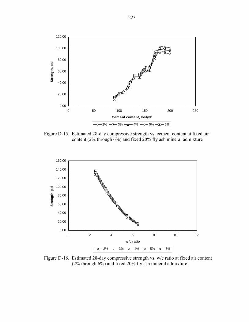
223
0.00
20.00
40.00
60.00
80.00
100.00
120.00
0 50 100 150 200 250
Cement content, lbs/yd3
Stre
ngth
, psi
2% 3% 4% 5% 6%
Figure D-15. Estimated 28-day compressive strength vs. cement content at fixed air content (2% through 6%) and fixed 20% fly ash mineral admixture
0.00
20.00
40.00
60.00
80.00
100.00
120.00
140.00
160.00
0 2 4 6 8 10 12
w/c ratio
Stre
ngth
, psi
2% 3% 4% 5% 6%
Figure D-16. Estimated 28-day compressive strength vs. w/c ratio at fixed air content (2% through 6%) and fixed 20% fly ash mineral admixture

224
0.00
50.00
100.00
150.00
200.00
250.00
0 50 100 150 200 250
Cement content, lbs/yd3
Stre
ngth
, LB
R
7% 8% 9% 10% 11%
Figure D-17. Estimated 28-day LBR strength vs. cement content at fixed air content (7% through 11%) and fixed 20% fly ash mineral admixture
0.00
50.00
100.00
150.00
200.00
250.00
0 2 4 6 8 10 12
w/c ratio
Stre
ngth
, LB
R
7% 8% 9% 10% 11%
Figure D-18. Estimated 28-day LBR strength vs. w/c ratio at fixed air content (7% through 11%) and fixed 20% fly ash mineral admixture

225
0.00
20.00
40.00
60.00
80.00
100.00
120.00
0 50 100 150 200 250
Cement content, lbs/yd3
Stre
ngth
, psi
7% 8% 9% 10% 11%
Figure D-19. Estimated 28-day compressive strength vs. cement content at fixed air content (7% through 11%) and fixed 20% fly ash mineral admixture
0.00
20.00
40.00
60.00
80.00
100.00
120.00
140.00
0 2 4 6 8 10 12
w/c ratio
Stre
ngth
, psi
7% 8% 9% 10% 11%
Figure D-20. Estimated 28-day compressive strength vs. w/c ratio at fixed air content (7% through 11%) and fixed 20% fly ash mineral admixture

226
0.00
20.00
40.00
60.00
80.00
100.00
120.00
140.00
160.00
0 50 100 150 200 250
Cement content, lbs/yd3
Stre
ngth
, LB
R
12% 13% 14% 15%
Figure D-21. Estimated 28-day LBR strength vs. cement content at fixed air content (12% through 15%) and fixed 20% fly ash mineral admixture
0.00
20.00
40.00
60.00
80.00
100.00
120.00
140.00
160.00
180.00
0 2 4 6 8 10 12
w/c ratio
Stre
ngth
, LB
R
12% 13% 14% 15%
Figure D-22. Estimated 28-day LBR strength vs. w/c ratio at fixed air content (12% through 15%) and fixed 20% fly ash mineral admixture

227
0.00
10.00
20.00
30.00
40.00
50.00
60.00
70.00
80.00
90.00
100.00
0 50 100 150 200 250
Cement content, lbs/yd3
Stre
ngth
, psi
12% 13% 14% 15%
Figure D-23. Estimated 28-day compressive strength vs. cement content at fixed air content (12% through 15%) and fixed 20% fly ash mineral admixture
0.00
20.00
40.00
60.00
80.00
100.00
120.00
0 2 4 6 8 10 12
w/c ratio
Stre
ngth
, psi
12% 13% 14% 15%
Figure D-24. Estimated 28-day compressive strength vs. w/c ratio at fixed air content (12% through 15%) and fixed 20% fly ash mineral admixture

228
0.00
50.00
100.00
150.00
200.00
250.00
300.00
0 50 100 150 200 250
Cement content, lbs/yd3
Stre
ngth
, LB
R
2% 3% 4% 5% 6%
Figure D-25. Estimated 28-day LBR strength vs. cement content at fixed air content (2%
through 6%) and fixed 50% ground granulated blast-furnace slag mineral admixture
0.00
50.00
100.00
150.00
200.00
250.00
300.00
350.00
0 2 4 6 8 10 12
w/c ratio
Stre
ngth
, LB
R
2% 3% 4% 5% 6%
Figure D-26. Estimated 28-day LBR strength vs. w/c ratio at fixed air content (2% through 6%) and fixed 50% ground granulated blast-furnace slag mineral admixture

229
0.00
20.00
40.00
60.00
80.00
100.00
120.00
140.00
0 50 100 150 200 250
Cement content, lbs/yd3
Stre
ngth
, psi
2% 3% 4% 5% 6%
Figure D-27. Estimated 28-day compressive strength vs. cement content at fixed air content (2% through 6%) and fixed 50% ground granulated blast-furnace slag mineral admixture
0.00
20.00
40.00
60.00
80.00
100.00
120.00
140.00
160.00
180.00
0 2 4 6 8 10 12
w/c ratio
Stre
ngth
, psi
2% 3% 4% 5% 6%
Figure D-28. Estimated 28-day compressive strength vs. w/c ratio at fixed air content (2% through 6%) and fixed 50% ground granulated blast-furnace slag mineral admixture

230
0.00
50.00
100.00
150.00
200.00
250.00
0 50 100 150 200 250
Cement content, lbs/yd3
Stre
ngth
, LB
R
7% 8% 9% 10% 11%
Figure D-29. Estimated 28-day LBR strength vs. cement content at fixed air content (7% through 11%) and fixed 50% ground granulated blast-furnace slag mineral admixture
0
50
100
150
200
250
300
0 2 4 6 8 10 12
w/c ratio
Stre
ngth
, LB
R
7% 8% 9% 10% 11%
Figure D-30. Estimated 28-day LBR strength vs. w/c ratio at fixed air content (7% through 11%) and fixed 50% ground granulated blast-furnace slag mineral admixture

231
0.00
20.00
40.00
60.00
80.00
100.00
120.00
140.00
0 50 100 150 200 250
Cement content, lbs/yd3
Stre
ngth
, psi
7% 8% 9% 10% 11%
Figure D-31. Estimated 28-day compressive strength vs. cement content at fixed air content (7% through 11%) and fixed 50% ground granulated blast-furnace slag mineral admixture
0.00
20.00
40.00
60.00
80.00
100.00
120.00
140.00
160.00
0 2 4 6 8 10 12
w/c ratio
Stre
ngth
, psi
7% 8% 9% 10% 11%
Figure D-32. Estimated 28-day compressive strength vs. w/c ratio at fixed air content (7% through 11%) and fixed 50% ground granulated blast-furnace slag mineral admixture

232
0.00
50.00
100.00
150.00
200.00
250.00
0 50 100 150 200 250
Cement content, lbs/yd3
Stre
ngth
, LB
R
12% 13% 14% 15%
Figure D-33. Estimated 28-day LBR strength vs. cement content at fixed air content (12% through 15%) and fixed 50% ground granulated blast-furnace slag mineral admixture
0
50
100
150
200
250
0 2 4 6 8 10 12
w/c ratio
Stre
ngth
, LB
R
12% 13% 14% 15%
Figure D-34. Estimated 28-day LBR strength vs. w/c ratio at fixed air content (12% through 15%) and fixed 50% ground granulated blast-furnace slag mineral admixture

233
0.00
20.00
40.00
60.00
80.00
100.00
120.00
0 50 100 150 200 250
Cement content, lbs/yd3
Stre
ngth
, psi
12% 13% 14% 15%
Figure D-35. Estimated 28-day compressive strength vs. cement content at fixed air content (12% through 15%) and fixed 50% ground granulated blast-furnace slag mineral admixture
0
20
40
60
80
100
120
140
0 2 4 6 8 10 12
w/c ratio
Stre
ngth
, psi
12% 13% 14% 15%
Figure D-36. Estimated 28-day compressive strength vs. w/c ratio at fixed air content (12% through 15%) and fixed 50% ground granulated blast-furnace slag mineral admixture

234
0.00
50.00
100.00
150.00
200.00
250.00
300.00
350.00
0 50 100 150 200 250
Cement content, lbs/yd3
Stre
ngth
, LB
R
2% 3% 4% 5% 6%
Figure D-37. Estimated 56-day LBR strength vs. cement content at fixed air content (2% through 6%) and fixed 0% mineral admixture
0.00
50.00
100.00
150.00
200.00
250.00
300.00
350.00
0 2 4 6 8 10 12
w/c ratio
Stre
ngth
, LB
R
2% 3% 4% 5% 6%
Figure D-38. Estimated 56-day LBR strength vs. w/c ratio at fixed air content (2% through 6%) and fixed 0% mineral admixture
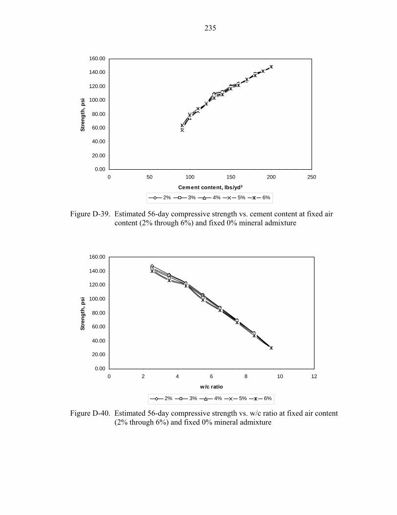
235
0.00
20.00
40.00
60.00
80.00
100.00
120.00
140.00
160.00
0 50 100 150 200 250
Cement content, lbs/yd3
Stre
ngth
, psi
2% 3% 4% 5% 6%
Figure D-39. Estimated 56-day compressive strength vs. cement content at fixed air
content (2% through 6%) and fixed 0% mineral admixture
0.00
20.00
40.00
60.00
80.00
100.00
120.00
140.00
160.00
0 2 4 6 8 10 12
w/c ratio
Stre
ngth
, psi
2% 3% 4% 5% 6%
Figure D-40. Estimated 56-day compressive strength vs. w/c ratio at fixed air content (2% through 6%) and fixed 0% mineral admixture

236
0.00
50.00
100.00
150.00
200.00
250.00
300.00
0 50 100 150 200 250
Cement content, lbs/yd3
Stre
ngth
, LB
R
7% 8% 9% 10% 11%
Figure D-41. Estimated 56-day LBR strength vs. cement content at fixed air content (7% through 11%) and fixed 0% mineral admixture
0.00
50.00
100.00
150.00
200.00
250.00
300.00
0 2 4 6 8 10 12
w/c ratio
Stre
ngth
, LB
R
7% 8% 9% 10% 11%
Figure D-42. Estimated 56-day LBR strength vs. w/c ratio at fixed air content (7% through 11%) and fixed 0% mineral admixture
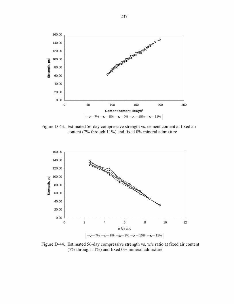
237
0.00
20.00
40.00
60.00
80.00
100.00
120.00
140.00
160.00
0 50 100 150 200 250
Cement content, lbs/yd3
Stre
ngth
, psi
7% 8% 9% 10% 11%
Figure D-43. Estimated 56-day compressive strength vs. cement content at fixed air
content (7% through 11%) and fixed 0% mineral admixture
0.00
20.00
40.00
60.00
80.00
100.00
120.00
140.00
160.00
0 2 4 6 8 10 12
w/c ratio
Stre
ngth
, psi
7% 8% 9% 10% 11%
Figure D-44. Estimated 56-day compressive strength vs. w/c ratio at fixed air content (7% through 11%) and fixed 0% mineral admixture

238
0.00
50.00
100.00
150.00
200.00
250.00
0 50 100 150 200 250
Cement content, lbs/yd3
Stre
ngth
, LB
R
12% 13% 14% 15%
Figure D-45. Estimated 56-day LBR strength vs. cement content at fixed air content (12% through 15%) and fixed 0% mineral admixture
0.00
50.00
100.00
150.00
200.00
250.00
0 2 4 6 8 10 12
w/c ratio
Stre
ngth
, LB
R
12% 13% 14% 15%
Figure D-46. Estimated 56-day LBR strength vs. w/c ratio at fixed air content (12% through 15%) and fixed 0% mineral admixture
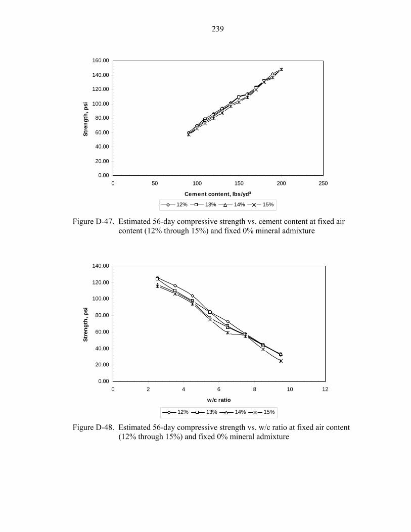
239
0.00
20.00
40.00
60.00
80.00
100.00
120.00
140.00
160.00
0 50 100 150 200 250
Cement content, lbs/yd3
Stre
ngth
, psi
12% 13% 14% 15%
Figure D-47. Estimated 56-day compressive strength vs. cement content at fixed air
content (12% through 15%) and fixed 0% mineral admixture
0.00
20.00
40.00
60.00
80.00
100.00
120.00
140.00
0 2 4 6 8 10 12
w/c ratio
Stre
ngth
, psi
12% 13% 14% 15%
Figure D-48. Estimated 56-day compressive strength vs. w/c ratio at fixed air content (12% through 15%) and fixed 0% mineral admixture
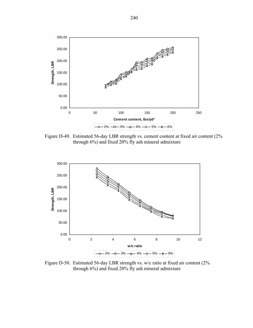
240
0.00
50.00
100.00
150.00
200.00
250.00
300.00
0 50 100 150 200 250
Cement content, lbs/yd3
Stre
ngth
, LB
R
2% 3% 4% 5% 6%
Figure D-49. Estimated 56-day LBR strength vs. cement content at fixed air content (2% through 6%) and fixed 20% fly ash mineral admixture
0.00
50.00
100.00
150.00
200.00
250.00
300.00
0 2 4 6 8 10 12
w/c ratio
Stre
ngth
, LB
R
2% 3% 4% 5% 6%
Figure D-50. Estimated 56-day LBR strength vs. w/c ratio at fixed air content (2% through 6%) and fixed 20% fly ash mineral admixture

241
0.00
20.00
40.00
60.00
80.00
100.00
120.00
140.00
0 50 100 150 200 250
Cement content, lbs/yd3
Stre
ngth
, psi
2% 3% 4% 5% 6%
Figure D-51. Estimated 56-day compressive strength vs. cement content at fixed air content (2% through 6%) and fixed 20% fly ash mineral admixture
0.00
20.00
40.00
60.00
80.00
100.00
120.00
140.00
0 2 4 6 8 10 12
w/c ratio
Stre
ngth
, psi
2% 3% 4% 5% 6%
Figure D-52. Estimated 56-day compressive strength vs. w/c ratio at fixed air content (2% through 6%) and fixed 20% fly ash mineral admixture

242
0.00
50.00
100.00
150.00
200.00
250.00
0 50 100 150 200 250
Cement content, lbs/yd3
Stre
ngth
, LB
R
7% 8% 9% 10% 11%
Figure D-53. Estimated 56-day LBR strength vs. cement content at fixed air content (7% through 11%) and fixed 20% fly ash mineral admixture
0.00
50.00
100.00
150.00
200.00
250.00
0 2 4 6 8 10 12
w/c ratio
Stre
ngth
, LB
R
7% 8% 9% 10% 11%
Figure D-54. Estimated 56-day LBR strength vs. w/c ratio at fixed air content (7% through 11%) and fixed 20% fly ash mineral admixture

243
0.00
20.00
40.00
60.00
80.00
100.00
120.00
140.00
0 50 100 150 200 250
Cement content, lbs/yd3
Stre
ngth
, psi
7% 8% 9% 10% 11%
Figure D-55. Estimated 56-day compressive strength vs. cement content at fixed air content (7% through 11%) and fixed 20% fly ash mineral admixture
0.00
20.00
40.00
60.00
80.00
100.00
120.00
140.00
0 2 4 6 8 10 12
w/c ratio
Stre
ngth
, psi
7% 8% 9% 10% 11%
Figure D-56. Estimated 56-day compressive strength vs. w/c ratio at fixed air content (7% through 11%) and fixed 20% fly ash mineral admixture

244
0.00
50.00
100.00
150.00
200.00
250.00
0 50 100 150 200 250
Cement content, lbs/yd3
Stre
ngth
, LB
R
12% 13% 14% 15%
Figure D-57. Estimated 56-day LBR strength vs. cement content at fixed air content (12% through 15%) and fixed 20% fly ash mineral admixture
0.00
20.00
40.00
60.00
80.00
100.00
120.00
140.00
160.00
180.00
200.00
0 2 4 6 8 10 12
w/c ratio
Stre
ngth
, LB
R
12% 13% 14% 15%
Figure D-58. Estimated 56-day LBR strength vs. w/c ratio at fixed air content (12% through 15%) and fixed 20% fly ash mineral admixture

245
0.00
20.00
40.00
60.00
80.00
100.00
120.00
140.00
0 50 100 150 200 250
Cement content, lbs/yd3
Stre
ngth
, psi
12% 13% 14% 15%
Figure D-59. Estimated 56-day compressive strength vs. cement content at fixed air content (12% through 15%) and fixed 20% fly ash mineral admixture
0.00
20.00
40.00
60.00
80.00
100.00
120.00
0 2 4 6 8 10 12
w/c ratio
Stre
ngth
, psi
12% 13% 14% 15%
Figure D-60. Estimated 56-day compressive strength vs. w/c ratio at fixed air content (12% through 15%) and fixed 20% fly ash mineral admixture

246
0.00
50.00
100.00
150.00
200.00
250.00
300.00
350.00
0 50 100 150 200 250
Cement content, lbs/yd3
Stre
ngth
, LB
R
2% 3% 4% 5% 6%
Figure D-61. Estimated 56-day LBR strength vs. cement content at fixed air content (2% through 6%) and fixed 50% ground granulated blast-furnace slag mineral admixture
0.00
50.00
100.00
150.00
200.00
250.00
300.00
350.00
0 2 4 6 8 10 12
w/c ratio
Stre
ngth
, LB
R
2% 3% 4% 5% 6%
Figure D-62. Estimated 56-day LBR strength vs. w/c ratio at fixed air content (2% through 6%) and fixed 50% ground granulated blast-furnace slag mineral admixture

247
0.00
20.00
40.00
60.00
80.00
100.00
120.00
140.00
160.00
0 50 100 150 200 250
Cement content, lbs/yd3
Stre
ngth
, psi
2% 3% 4% 5% 6%
Figure D-63. Estimated 56-day compressive strength vs. cement content at fixed air content (2% through 6%) and fixed 50% ground granulated blast-furnace slag mineral admixture
0.00
20.00
40.00
60.00
80.00
100.00
120.00
140.00
160.00
0 2 4 6 8 10 12
w/c ratio
Stre
ngth
, psi
2% 3% 4% 5% 6%
Figure D-64. Estimated 56-day compressive strength vs. w/c ratio at fixed air content (2% through 6%) and fixed 50% ground granulated blast-furnace slag mineral admixture
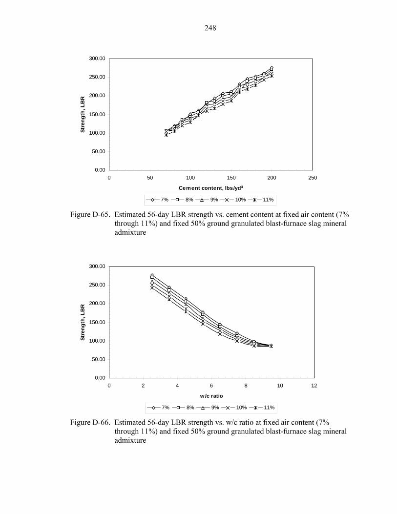
248
0.00
50.00
100.00
150.00
200.00
250.00
300.00
0 50 100 150 200 250
Cement content, lbs/yd3
Stre
ngth
, LB
R
7% 8% 9% 10% 11%
Figure D-65. Estimated 56-day LBR strength vs. cement content at fixed air content (7% through 11%) and fixed 50% ground granulated blast-furnace slag mineral admixture
0.00
50.00
100.00
150.00
200.00
250.00
300.00
0 2 4 6 8 10 12
w/c ratio
Stre
ngth
, LB
R
7% 8% 9% 10% 11%
Figure D-66. Estimated 56-day LBR strength vs. w/c ratio at fixed air content (7% through 11%) and fixed 50% ground granulated blast-furnace slag mineral admixture

249
0.00
20.00
40.00
60.00
80.00
100.00
120.00
140.00
160.00
0 50 100 150 200 250
Cement content, lbs/yd3
Stre
ngth
, psi
7% 8% 9% 10% 11%
Figure D-67. Estimated 56-day compressive strength vs. cement content at fixed air content (7% through 11%) and fixed 50% ground granulated blast-furnace slag mineral admixture
0.00
20.00
40.00
60.00
80.00
100.00
120.00
140.00
160.00
0 2 4 6 8 10 12
w/c ratio
Stre
ngth
, psi
7% 8% 9% 10% 11%
Figure D-68. Estimated 56-day compressive strength vs. w/c ratio at fixed air content (7% through 11%) and fixed 50% ground granulated blast-furnace slag mineral admixture

250
0.00
50.00
100.00
150.00
200.00
250.00
300.00
0 50 100 150 200 250
Cement content, lbs/yd3
Stre
ngth
, LB
R
12% 13% 14% 15%
Figure D-69. Estimated 56-day LBR strength vs. cement content at fixed air content (12% through 15%) and fixed 50% ground granulated blast-furnace slag mineral admixture
0
50
100
150
200
250
0 2 4 6 8 10 12
w/c ratio
Stre
ngth
, LB
R
12% 13% 14% 15%
Figure D-70. Estimated 56-day LBR strength vs. w/c ratio at fixed air content (12% through 15%) and fixed 50% ground granulated blast-furnace slag mineral admixture

251
0.00
20.00
40.00
60.00
80.00
100.00
120.00
140.00
160.00
0 50 100 150 200 250
Cement content, lbs/yd3
Stre
ngth
, psi
12% 13% 14% 15%
Figure D-71. Estimated 56-day compressive strength vs. cement content at fixed air content (12% through 15%) and fixed 50% ground granulated blast-furnace slag mineral admixture
0
20
40
60
80
100
120
140
0 2 4 6 8 10 12
w/c ratio
Stre
ngth
, psi
12% 13% 14% 15%
Figure D-72. Estimated 56-day compressive strength vs. w/c ratio at fixed air content (12% through 15%) and fixed 50% ground granulated blast-furnace slag mineral admixture

252
LIST OF REFERENCES
1. Jawed, I., and Skalny, J., Hardened Mortar and Concrete with Fly Ash, Fly Ash in
Concrete, K. Wesche, ed., E&FN Spon, Great Britain, 1991.
2. Popovic, S., Concrete Making Materials, Hemisphere Publishing Company, New York, NY, 1979.
3. Pons, F., Landwermeyer, J. S., and Kerns, L., “Development of Engineering Properties for Regular and Quick-Set Flowable Fill,” The Design and Application of Controlled Low-Strength Materials (Flowable Fill), ASTM STP 1331, A. K. Howard and J. L. Hitch, eds., American Society for Testing and Materials, West Conshohocken, PA, 1998.
4. Digioia, Jr., A. M., and Brenda, G. F., Fly Ash Design Manual for Road and Site Applications, Vol. 2: Slurried Placement, EPRI Report Tr-100472, Electric and Power Research Institute, Palo Alto, CA, 1992.
5. Du, L., Folliard, K. J., and Trejo, D., “Effects of Constituent Materials and Quantities on Water Demand and Compressive Strength of Controlled Low-Strength Material,” Journal of Materials in Civil Engineering, ASCE Publications, Reston, VA, November/ December 2002.
6. American Concrete Institute (ACI) Committee 229, “ACI 229R-94 Report: Controlled Low Strength Materials (CLSM),” Concrete International, Vol. 16, No. 7, Farmington Hills, MI, July, 1994, p. 55-64.
7. Grandham, S., Seals, R. K. and Fox worthy, P. T., “Phosphogypsum as a component of flowable fill,” Transportation Research Record, No. 1546, 1996.
8. Florida Concrete and Products Association, Inc., Flowable Fill Demonstration, RMC 2000, Orlando, FL, 2003.
9. Naik, T. R., Kraus, R. N., Sturzl, R. F., and Ramme, B. W., “Design and Testing Controlled Low-Strength Materials (CLSM) Using Clean Coal Ash,” The Design and Application of Controlled Low-Strength Materials (Flowable Fill), ASTM STP 1331, A. K. Howard and J. L. Hitch, eds., American Society for Testing and Materials, West Conshohocken, PA, 1998.

253
10. Webb, M. C., McGrath, T. J., and Selig, E. T., “Field Test of Buried Pipe with CLSM Backfill,” The Design and Application of Controlled Low-Strength Materials (Flowable Fill), ASTM STP 1331, A. K. Howard and J. L. Hitch, eds., American Society for Testing and Materials, West Conshohocken, PA, 1998.
11. Howard, A. K., “Proposed Standard Practice for Installing Buried Pipe Using Flowable Fill,” The Design and Application of Controlled Low-Strength Materials (Flowable Fill), ASTM STP 1331, A. K. Howard and J. L. Hitch, eds., American Society for Testing and Materials, West Conshohocken, PA, 1998.
12. Riggs, E. H., and Keck, R. H., “Specifications and Use of Controlled Low-Strength Material by State Transportation Agencies,” The Design and Application of Controlled Low-Strength Materials (Flowable Fill), ASTM STP 1331, A. K. Howard and J. L. Hitch, eds., American Society for Testing and Materials, West Conshohocken, PA, 1998.
13. Baker, T. H. W., “Frost Penetration in Flowable Fill Used in Pipe Trench Backfill,” The Design and Application of Controlled Low-Strength Materials (Flowable Fill), ASTM STP 1331, A. K. Howard and J. L. Hitch, eds., American Society for Testing and Materials, West Conshohocken, PA, 1998.
14. Hitch, J. L., “Test Methods for Controlled Low-Strength Material (CLSM): Past, Present, and Future,” The Design and Application of Controlled Low-Strength Materials (Flowable Fill), ASTM STP 1331, A. K. Howard and J. L. Hitch, eds., American Society for Testing and Materials, West Conshohocken, PA, 1998.
15. American Association of State Highway and Transportation Officials (AASHTO), Standard Specifications for Transportation Materials and Methods of Sampling and Testing, Seventeenth Edition, Part 1 Specifications, Washington, D.C., 1995.
16. Florida Department of Transportation (FDOT), “Standard Specifications for Road and Bridge Construction,” Flowable Fill Specifications, Section 121, FDOT Map and Publication Sales, Tallahassee, FL, 2000.
17. Kendall, K., Interparticle Friction in Slurries, Tribology in Particulate Technology, B. J. Briscoe and M. J. Adams Hilger, ed., Bristol, England, 1987.
18. Popovic, S., Fundamentals of Portland Cement Concrete: A Quantitative Approach, Vol. 1: Fresh Concrete, John Wiley & Sons, New York, NY, 1982.
19. Soroka, I., Portland Cement Paste and Concrete, Chemical Publishing Co., Inc., New York, NY, 1979.
20. Rixom, M. R., and Mailvaganam, N. P, Chemical Admixtures for Concrete, E&FN Spon, Great Britain, 1986.
21. Neville, A. M., Properties of Concrete, 4th edition, John Wiley and Sons, Inc., New York, NY, 1998.

254
22. Diamond, S., “Cement Paste Microstructure in Concrete,” Materials Research Society Proceedings, Materials Research Society, Warrendale, PA, Vol. 85, 1987.
23. Helmuth, R., Fly Ash in Cement and Concrete, Portland Cement Association, Skokie, IL, 1987.
24. Halverson, R.R., B. Boggs, J. Enyart, and G. Madden., “Accelerated non-pozzolanic reactions of high volume coal fly ash concrete.” Proceedings of the 14th
International Symposium on Management and Use of Coal Combustion Products. Provided courtesy of the American Coal Ash Association: Alexandria, VA., 2001
25. Ledesma, R. and L.L. Isaacs., “Thermal properties of coal ashes,” Fly Ash and Coal Conversion By-Products: Characterization, Utilization and Disposal VI. Robert L. Day and Fredrik Pl. Glasser, eds., Materials Research Society: Pittsburgh, Pennsylvania., 1990
26. Turner-Fairbank Highway Research Center (TFHRC)., “User Guidelines for Waste and Byproduct Materials in Pavement Construction.” <http://ww.tfhrc.gov/hnr20/recycle/waste/index.htm> (June 02, 2004).
27. McCarthy, G.J., J.K. Solem, O.E. Manz, and D.J. Hassett., “Use of a database of chemical, mineralogical, and physical properties of North American fly ash to study the nature of fly ash and its utilization as a mineral admixture in concrete.” Fly Ash and Coal Conversion By-Products: Characterization, Utilization and Disposal VI. Robert L. Day and Fredrik Pl. Glasser, eds., Materials Research Society: Pittsburgh, Pennsylvania., 1990
28. Joshi, R. C., and Lohtia, R. P., Fly Ash in Concrete: Production, Properties and Uses, Vol. 2: Advances in Concrete Technology, Gordon and Breach Science Publishers, Ontario, Canada, 1997.
29. Popovic, S., Fundamentals of Portland Cement Concrete: A Quantitative Approach, Vol. 1: Fresh Concrete. John Wiley & Sons., Hoboken, NJ., 1982
30. Swanekamp, R., “Disposal and reuse of coal combustion byproducts,” Power Magazine 146, Houston, Texas, July 2002, p.37-41.
31. Boral Material Technologies, “Boral ® Class F Fly Ash,” Product Brochure. San Antonio, TX., 2000
32. Stewart, B.R., “Coal combustion product (CCP) production and use.” Biogeochemistry of Trace Elements in Coal and Coal Combustion Byproducts. Kenneth S. Sajwan, Ashok K. Alva, and Robert F. Keefer, eds. Kluwer Academic/Plenum Publishers: New York, NY., 1999
33. ACI Committee 233R, “Ground Granulated Blast-Furnace Slag as a Cementitious Constituent in Concrete,” American Concrete Institute, Farmington Hills, Mich., 1995.

255
34. Roy, D. M., and Idorn, G. M.,”Hydration, Structure, and Properties of Blast Furnace Slag Cements, Mortars, and Concrete,” ACI Journal, Proceedings, V. 79, No. 6, Nov-Dec. 1982, pp. 445-457.
35. Mindess, S., and Young, J. F, Concrete, Prentice-Hall Inc., Englewood Cliffs, NJ, 1981.
36. Hamilton County and the City of Cincinnati, “A Performance Specification for Controlled Low Strength Material, Controlled Density Fills (CLSM-CDF),” Report, Cincinnati, OH, 1996.
37. Bhat, S. T, “Use of Coal Combustion Residues and Foundry Sands in Flowable Fill,” Ph.D. Dissertation, Purdue University, West Lafayette, IN, 1996.
38. Folliard, K. J., Trejo, D., Sabol, S. A., and Du., L., “Controlled Low-Strength Material for Backfill, Utility Bedding, Void Fill and Bridge Approaches,” Phase I Interim Report 24-12, National Cooperative Highway Research Program (NCHRP), 1999.
39. Najafi, F. T., and Tia, M., Use of Accelerated Flowable Fill in Pavement Section, Florida Department of Transportation, Tallahassee, FL, 2004.
40. Montgomery, D. C., Design and Analysis of Experiments, 5th edition, John Wiley and Sons, Inc., New York, NY, 2001.
41. Oehlert, G. W., A First Course in Design and Analysis of Experiments, W. H. Freeman and Company, New York, NY, 2000.
42. Florida Department of Transportation (FDOT), Lime Rock Bearing Ratio Technician Certification Study Guide, 1986 Edition, Tallahassee, FL, 1986.
43. Lucht, D.A., Thermal Performance of Flowable Fill Mixtures for Horizontal GSHP Systems, M.S. Thesis, South Dakota State University, 1995.
44. Kosmatka, S. H., and Panarese, W. C., Design and Control of Concrete Mixtures, 13th edition, Portland Cement Association, Skokie, IL, 1994.
45. Bhat, S. T., and Lovell, C. W., “Design of Flowable Fill: Waste Foundry Sand as a Fine Aggregate,” Transportation Research Record 1546, Transportation Research Board, National Research Council, Washington, D.C., 1996.
46. Lerch, W., “Basic Principles of Air-Entrained Concrete,” Portland Cement Association Special Report, Skokie, IL, 1960.
47. Natrella, M. G., Experimental Statistics, NBS Handbook 91, National Bureau of Standards, Washington, D.C., 1963.
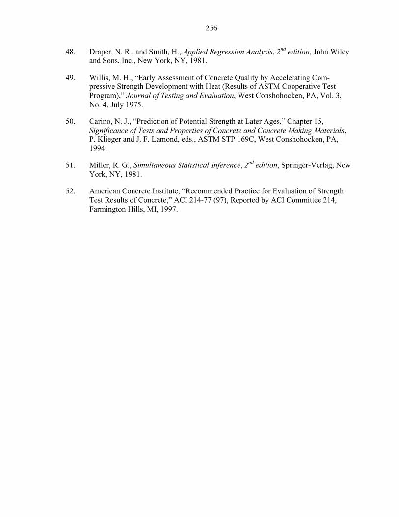
256
48. Draper, N. R., and Smith, H., Applied Regression Analysis, 2nd edition, John Wiley and Sons, Inc., New York, NY, 1981.
49. Willis, M. H., “Early Assessment of Concrete Quality by Accelerating Com-pressive Strength Development with Heat (Results of ASTM Cooperative Test Program),” Journal of Testing and Evaluation, West Conshohocken, PA, Vol. 3, No. 4, July 1975.
50. Carino, N. J., “Prediction of Potential Strength at Later Ages,” Chapter 15, Significance of Tests and Properties of Concrete and Concrete Making Materials, P. Klieger and J. F. Lamond, eds., ASTM STP 169C, West Conshohocken, PA, 1994.
51. Miller, R. G., Simultaneous Statistical Inference, 2nd edition, Springer-Verlag, New York, NY, 1981.
52. American Concrete Institute, “Recommended Practice for Evaluation of Strength Test Results of Concrete,” ACI 214-77 (97), Reported by ACI Committee 214, Farmington Hills, MI, 1997.

257
BIOGRAPHICAL SKETCH
Webert Lovencin was born on Monday, December 25, 1972, in Hatte Cheveâux,
Haiti, to Ms. Elvira Lovencin and Mr. Nicholas J. Pierre. In July 1982, he moved to the
United States and attended Edison Park Elementary School, Edison Middle School, and
Edison Senior High School in Miami, Florida. He graduated from Miami Edison Senior
High School in June 1991. After graduating from high school he attended the University
of Florida (UF). At UF, he earned a Bachelor of Science degree in Civil Engineering in
May 1997. He also received a Master of Engineering degree in August 1999 specializing
in the area of transportation engineering. His research for this degree was titled “An
Investigation of Red Light Running in the City of Gainesville, Florida.” Thereafter, he
enrolled in a Doctor of Philosophy (Ph.D.) program specializing in public works/con-
struction management and materials in the Department of Civil and Coastal Engineering
at UF.
After a one-year stint of working on his Ph.D. full time, Mr. Lovencin obtained a
position with the Florida Department of Transportation (District 2) as a Professional
Engineer Trainee. This two-year program consisted of various phases to provide
experience in the many areas of the transportation field. After completing this program,
he entered into the Senior Engineer Trainee Program which consisted of specialized
training in the area of construction management. While working for the Florida
Department of Transportation, he continued to pursue his graduate studies until he was

258
awarded an “Educational Leave with Pay” by the Department to continue his studies full-
time.
Mr. Lovencin was married on July 15, 2000, to the former April Adrienne Raines.
After completing his Ph.D., Webert Lovencin plans to continue to work for the Florida
Department of Transportation.