assessing the adjustment implications of trade policy...
TRANSCRIPT

1
Assessing the Adjustment Implications of Trade Policy Changes Using TRIST
(Tariff Reform Impact Simulation Tool) 1
Authors:
Paul Brenton, Christian Saborowski, Cornelia Staritz and Erik von Uexkull
This Draft: August 2009
Abstract TRIST is a simple, easy to use tool to assess the adjustment implications of trade reform. It
improves on existing tools. First, it is an improvement in terms of accuracy because projections
are based on revenues actually collected at the tariff line level rather than simply applying
statutory rates. Second, it is transparent and open; runs in Excel, with formulas and calculation
steps visible to the user; and is open-source and users are free to change, extend, or improve
according to their needs. Third, TRIST has greater policy relevance because it projects the impact
of tariff reform on total fiscal revenue (including VAT and excise) and results are broken down to
the product level so that sensitive products or sectors can be identified. And fourth, the tool is
flexible and can incorporate tariff liberalization scenarios involving any group of trading partners
and any schedules of products. This paper describes the TRIST tool and provides a range of
examples that demonstrate the insights that the tool can provide to policy makers on the
adjustment impacts of reducing tariffs.
1 We would like to thank Ian Gillson, Anneke Hamilton, Bernard Hoekman, Jamus Jerome Lim, Juan
Sebastian Saez, Philip Schuler, David Tarr and Peter Walkenhorst for valuable comments. TRIST is a
product of the World Bank‟s International Trade Department. It was initially developed by Mombert Hoppe
and Erik von Uexkull under the leadership of Paul Brenton. The development and design of the revised
version was led by Paul Brenton and coordinated by Christian Saborowski and Erik von Uexkull. Olivier
Jammes contributed to the design of the revised version and was responsible for its technical
implementation. Cornelia Staritz contributed to the extension of the tool to output and employment
analysis. The recently launched revised version of TRIST has benefited from valuable inputs from
colleagues both within and outside the World Bank, including Ian Gillson (World Bank Africa Region),
Soamiely Andriamananjara (World Bank Institute), Themba Munalula (COMESA secretariat), Caesar
Cheelo (University of Zambia), Peter Walkenhorst (AfDB), discussions with TRIST seminar participants in
Bolivia, Ethiopia, Seychelles, Syria, Tanzania, Malawi, Mauritius, Nigeria and Zambia, and presentations
at the COMESA secretariat (Lusaka), the EAC secretariat (Arusha), UNECA (Addis Ababa), and at the
World Bank. The TRIST team acknowledges financial support for TRIST from the governments of
Finland, Norway, Sweden and the United Kingdom through the Multidonor Trust Fund for Trade and
Development. The views expressed here are those of the authors and should not be attributed to the World
Bank. All correspondence regarding TRIST or related activities should be directed to Christian Saborowksi
2
1. Introduction
Careful analysis of the adjustment impacts of trade reform is essential to policy makers in
developing countries as they seek to improve the structure of incentives within an
outward looking trade and competitiveness strategy. The need to adjust will arise in a
number of areas. An immediate concern, especially in low-income countries, is the
impact on tax revenues. Tariffs are typically an important source of tax revenues in low-
income countries, often reflecting the weakness of the domestic tax base and of other tax
instruments. In addition, changes in output in different sectors and associated impacts on
employment are likely to be an important aspect of the political economy driving support
and opposition to trade reform. Further, trade reform entails changes in prices and an
important consideration is how these will affect households, especially the poorest. A
good understanding of the potential adjustment implications of trade reform can
contribute to the design of better trade reform strategies and to the discussion and
implementation of policies that can reduce the impact of adjustment, especially when the
costs are concentrated upon particular groups in society. The latter is of particular
importance in countries that lack social safety nets with broad coverage.
In response the World Bank has developed a simple spreadsheet tool called TRIST
(Tariff Reform Impact Simulation Tool) that can be used by policy makers in client
countries to analyze the adjustment implications of trade reform2. The tool was initially
developed to provide better estimates of the impact of changes in tariffs on government
revenues, imports, protection and prices. Unlike other tools it does not require any
proprietary software, programming skills or internet access. It is free and easy to use,
transparent, with a simple underlying trade model, and flexible, in that it can quickly
address different trade policy scenarios. It uses detailed data on actual revenues collected
from trade whereas other tools use hypothetical revenues from applying duty rates on
paper. It also includes all taxes levied on trade, not just tariffs, and so shows the change
in trade tax revenues, which is more relevant than the change in tariff revenues alone.
When suitable data are available, it can provide information on the short-term relative
vulnerability of different sectors in the domestic economy in terms of output and
employment.3 It can also be linked to household budget data to trace the influence of
changes in prices following trade reform to household expenditures and the costs of
attaining the given consumption bundle. The objective of the model is to assist policy
makers in identifying issues relating to adjustment to trade reform. It cannot provide an
assessment of whether a particular policy change is beneficial or not. This purpose would
require a more sophisticated economy-wide model.
2 Brenton et al (2007) describes the initial motivation, development and application of the model.
3 As discussed below, TRIST should not be used to project either the aggregate impact of tariff reform on
domestic production and employment. Given its nature as a partial equilibrium model, its purpose is rather
to identify sectors that are likely to be hardest hit as part of the direct short term adjustment to increased
competition in import markets and to contribute to the design of policy interventions that seek to cushion
these direct adjustment costs.

3
Low-income countries currently face a range of trade policy options and issues. First
there is the option for unilateral reforms to the trade regime, for example, to reduce, the
most distorting peak tariffs. Most countries are actively negotiating bilateral and regional
trade agreements. The African, Caribbean and Pacific countries are negotiating and
implementing Economic Partnership Agreements (EPAs) with the EU to replace the
previous Cotonou Agreement. An integral part of these agreements is preferential
reduction of tariffs against imports from the EU. Many African countries are involved in
initiatives towards regional free trade (COMESA, EAC, SADC, ECOWAS) and most of
these regional communities have plans to adopt a common external tariff. Finally, there is
the multilateral trade reform process centered on the WTO. All of these trade policy
options entail changes to revenues and implications for output, employment and poverty.
This paper provides a description of the TRIST tool and gives examples of its use.
Section 2 discusses the objective behind the development of TRIST and outlines crucial
advantages compared to existing tools. Section 3 presents the trade model underlying the
tool and discusses the intuition behind the calculation steps. In Section 4, some examples
of the analysis of short term adjustment costs are presented using TRIST. These comprise
both the main focus of TRIST, namely the simulation of fiscal adjustment costs of trade
policy reform, as well as the adjustment costs in terms of domestic production and
employment and the use of TRIST in the analysis of poverty and trade diversion. Section
5 concludes.
2. The Purpose of TRIST
The TRIST software follows the open source and country ownership principles in that it
is free of charge and independent use and development is strongly encouraged. The tool
is Excel based and does not require any additional proprietary software, hardware (other
than minimal disk space) or programming expertise. The origin of TRIST lies in the
limitations of existing tools in providing support to policy makers in developing countries
in assessing the implications of trade reforms. There are three main limitations of existing
tools and studies that TRIST seeks to overcome:
1. Most models use statutory tariffs (those on paper) and recorded trade flows. This can
lead to a lack of precision in predicted impacts since in practice large amounts of imports
are exempted from paying customs duties. A common feature of import regimes of
developing countries is the widespread use of tariff exemptions for various reasons. For
example, a range of institutions including the government, international agencies,
embassies and NGOs often do not pay duties on products imported for official purposes.
It is important that these imports are excluded since they do not enter the domestic
market in free circulation and can not be used for commercial purposes4. Exemptions are
4 The arguments for exempting international institutions and NGOs from customs duties are not
overwhelming and such a policy can lead to notable distortions. For example, countries often levy higher
tariffs and excises on cars with less fuel efficient engines. Being exempt from such duties may help explain
the large number of Toyota Land cruisers driven for personal use by the officials of international
institutions and NGOs in the capital cities of low income countries.

4
also granted to encourage exports by exempting duty on imported intermediate products
and to provide incentives for domestic and foreign investment. However, in practice the
efficacy of these exemptions in achieving these objectives is unclear, especially where
the granting of exemptions is opaque and discretionary in nature. Further, the existence of
exemptions not only diverts customs resources but may distort competition by favoring
some firms over others. Hence, it is important to take these exemptions into account and
assess their importance.5 In this regard, we estimated the potential tariff revenue increase
following the removal of all tariff exemptions and found that tariff revenue would
typically increase by around 40% to 50% in low income countries for which TRISTs
have been developed to date. These numbers illustrate that a better understanding of the
magnitude and structure of tariff exemptions is crucial in determining the adjustment
implications of tariff reform on fiscal revenues.
Using statutory rather than actually applied duties to investigate the impact of tariff
liberalization scenarios will therefore typically lead to a substantial overestimation of the
impact of tariff liberalization on trade flows and revenues. Table 1 shows how tariff and
total trade tax revenue in selected Common Market for Eastern and Southern Africa
(COMESA) countries would be affected by the removal of tariffs on imports from the EU
under an economic partnership agreement (EPA). In calculating revenue losses we make
use of data on actually collected rather than statutory tariff rates. We assume here that the
EPA entails reducing all tariffs on products imported from the EU to zero. In practice,
there are likely to be a range of products that are excluded that will reduce the revenue
effect, so that the estimates here will provide an upper bound on actual impacts6. Column
one in part A of the table shows that the predicted changes in tariff revenues mirror
closely the shares of EU imports in overall imports to each country being around 17% to
18% for Ethiopia and Zambia, 30% for Madagascar and 6% for Malawi. The next column
in part A presents the tariff revenue loss that would have been predicted had we used
statutory tariff rates to calculate the revenue changes as in previous studies. It is clear that
the predicted losses are now substantially higher. The final column in part A of Table 1
examines a scenario in which the respective countries attempt to recover the revenue loss
they incur due to the EPA by abolishing all tariff exemptions. The numbers show that the
resulting tariff revenue loss is much lower and there is even a gain in revenues in Zambia
and Malawi. This last point illustrates that, if addressed in a practical manner, the
sequenced reduction and abolition of tariff exemptions can allow countries to
significantly soften the revenue impact of tariff liberalization.
5 The use of collected rather than statutory revenue in the simulations also ensures that the impact of rules
of origin in practice is taken into account. 6 Because of data limitations for the countries under review, we assume the absence of a domestic
substitution effect between imports and domestic production (see below for a detailed discussion).

5
Table 1: Highlighting the Advantages of TRIST
A: Change in Tariff Revenue for an EPA (elimination of all tariffs on imports from the EU)
Based on collected tariffs Based on statutory tariffs Based on applied tariffs and
removal of all exemptions
Ethiopia -17.2% -32.6% -4.6%
Madagascar -29.9% -43.9% -12.1%
Malawi -6.5% -8.5% 26.2%
Zambia -17.7% -23.2% 24.6%
B: Change in Total Trade Tax Revenue for an EPA (elimination of all tariffs on imports from the EU)
Based on collected tariffs Based on statutory tariffs Based on applied tariffs and
removal of all exemptions
Ethiopia -3.4% -6.4% -0.8%
Madagascar -4.1% -5.6% -1.7%
Malawi -0.8% -1.1% 3.3%
Zambia -1.7% -2.3% 2.3%
1) The demand elasticity is set to 0.5, the exporter substitution elasticity is set to 1.5.
2) EPA scenario: zero tariffs with EU. For all other trading partners, tariffs are unchanged.
2. A second major challenge in investigating the impact of trade policy reform is to
account not only for statutory and applied tariff rates but also for the interplay between
tariffs and other forms of taxes collected at the border. Whilst duties from trade are a key
source of revenue in developing countries, customs duties are just one tax measure that is
applied at the border. Most countries also apply excise taxes as well as a VAT or sales
tax. Often these will generate significantly more revenue than customs duties. In fact, our
estimates show that in most countries tariff revenue constitutes substantially less than
50% of overall revenue collected at the border, e.g. Bolivia (20%), Kenya (25%),
Mozambique (32%) and Burundi (39%). Part B of Table 1 presents the impact of the
EPA policy scenario on overall import tax revenues. The proportionate changes are much
smaller, indicating that the magnitude of the trade tax revenue effect of trade
liberalization is, in percentage terms, significantly overstated when considering tariffs as
the only source of revenue.
In principle, unlike customs duties, both VAT and excise taxes are not distortionary since
they are applied to both domestic and foreign sources of supply. In practice, the domestic
tax base - for VAT in particular - tends to be very small in developing countries. Thus, it
is very important to take into account changes in VAT and excise receipts that follow the
reform of customs duties since it is total revenues from trade that are of interest to policy
makers. As tariffs are reduced and imports increase, revenues from other taxes will also
be affected. It is not ex-ante clear which sign the effect of trade liberalization on VAT
and excise revenue alone will take. It can be positive, due to increased imports, or
negative, due to a reduction of the tax base since VAT is usually levied on the tariff

6
inclusive value of imports. Either way, the percentage change in overall trade tax revenue
will be smaller than the impact on tariff revenue and studies that focus solely on changes
in customs duties will only provide a partial picture.
3. A third major motivation for the development of TRIST is the limitations that arise
from using aggregated and unwieldy models in a dynamic policy environment. New
options and proposals for trade policy emerge frequently and require adjustments to the
scenarios used for projections. Further, trade policy discussions typically concern detailed
products, such as identifying lists of sensitive products that are excluded from
liberalization scenarios. Thus, disaggregated results that break down the revenue impact
by detailed product and trading partner are a crucial input to trade policy formulation. An
important aim of TRIST is therefore to provide a simple and flexible tool that can be
easily and quickly used and adapted to reflect specific country circumstances as well as to
allow the user to define relevant reform scenarios, exclusion lists etc.
The EC Commission interpreted the GATT requirement that preferential trade
agreements such as EPAs lead to the gradual removal of tariffs and non-tariff barriers on
„substantially all trade‟ as allowing ACP countries to exempt up to 20% of their imports
from tariff reduction under an EPA.7 The detailed tariff line level data available in TRIST
allows policymakers to thoroughly analyze the implications of choosing different lists of
exempted products. In particular, countries may want to exclude products from
liberalization for which the policy reform will generate the largest reduction in revenue or
protection. To give a few examples, the projected tariff revenue loss from an EPA with
the EU falls from 14.4% to 2.1% in Tanzania, from 19.4% to 5.1% in Kenya and from
17.1% to 5.4% in Ethiopia when the sensitive product list is chosen according to the
revenue sensitivity of the products imported from the EU (see table 3). At the other
extreme, it is interesting to analyze the revenue impact of the reduction of very high
tariffs only since reducing such tariff peaks will remove an important distortion in the
7 The EC Commission interprets substantially all trade as covering 90% of mutual trade. Since the EU
countries will liberalize 100% of their imports from ACP countries under an EPA, the EC Commission has
deemed that the ACP countries must liberalize at least 80% of their imports from the EU.
Box 1: Advantages of TRIST
Accuracy: Projections are based on customs data on revenues (from tariffs, VAT, excise and other taxes applied at the border) actually collected at the tariff line level, broken down by user defined trading partner groups and
selected products. This improves the accuracy of tariff reform simulations by taking into account tariff exemptions and trading partner specific collection rates.
Transparency: The whole tool is set up in Excel and formulas and calculation steps are visible for the user. It is open-source in the sense that users are free to change, extend or improve according to their needs.
Simplicity: TRIST incorporates a simple partial equilibrium model of importing. The underlying modeling is
intuitive and simulations can be made by anyone within minutes once the appropriate tariff scenarios have been entered.
Policy Relevance: TRIST allows projecting the impact of tariff reform on total fiscal revenue (including VAT and excise) and results are broken down to the product level so sensitive products or sectors can be identified.
Flexibility: TRIST can incorporate tariff liberalization towards any group of trading partners. User defined tariff scenarios can be added, for example to incorporate a sensitive product list into the liberalization schedule. It is also
possible to enter multiple successive liberalization steps and project both their individual and cumulative impact.

7
importing regime of the economy. As an example, capping all tariffs at a maximum rate
of 25% is projected to result in moderate tariff (overall import) revenue losses of 0.5%
(0.1%), 3.8% (1.1%) and 10.1% (4.6%), in Zambia, Tanzania and Ethiopia respectively8.
The level of detail of the data used in TRIST as well as both the transparency and the
flexibility of the model have contributed to the widespread use of TRIST for the analysis
of policy relevant questions in client countries and ensured country ownership of the
results. TRISTs have to date been developed for Albania, Bolivia, Ethiopia, Jordan,
Kenya, Madagascar, Malawi, Mauritius, Morocco, Mozambique, Nigeria, Seychelles,
Syria, Tanzania, Tunisia and Zambia and a range of TRISTs are under construction.
In many circumstances, TRIST based simulations have contributed actively to policy
making. In Madagascar, policymakers decided to substantially reduce tariffs on capital
goods which had been high compared to regional competitors. This happened only after a
careful assessment of the revenue implications of the reform using TRIST, which
demonstrated that revenue losses would be much lower than initially expected. TRIST is
also the tool of choice for the COMESA secretariat to project revenue shares and to
estimate revenue losses emanating from trade reforms for which countries can
subsequently be compensated. In Nigeria, an analysis of the revenue implications of an
EPA with the EU (Andriamananjara et al, 2009) has found strong interest among high
level policymakers involved in the decision whether or not to engage in such an
agreement.
3. The Methodology Used in TRIST
TRIST is an Excel based tool that predicts the impact of tariff reform scenarios on the
basis of a simple partial equilibrium model. It consists of two Excel files: the first is the
Data Aggregation Tool which organizes and appropriately formats the data to be
imported into the second, the Simulation Tool. The Data Aggregation Tool allows the
user to create country and product groups that are relevant to the formulation of trade
policy scenarios in the country specific context. For example, the analysis of the revenue
implications of joining a free trade agreement (FTA) requires defining the members of
the FTA as a separate trading partner group. In the Simulation Tool the user defines the
tariff reform scenarios, can choose the parameters of the trade model underlying the
calculations, and reviews the simulation results both at the aggregate, the sectoral and at
the tariff line level.
In order to implement a TRIST for a given country, detailed and complete data on import
transactions for the most recent year is required (data averaged across a number of years
can also be used). For each import transaction, the data must identify the type of product
(tariff line level, typically HS 8 digit), the country of origin of the trade flow, the customs
procedure code (CPC) defining the customs regime under which the good enters the
8 For the simulations underlying the results presented in this paragraph a demand elasticity of 0.5 and an
exporter substitution elasticity of 1.5 were used.
8
country9, the import value of the transaction, the statutory tariff, the tariff actually applied
(to calculate tariff exemptions) as well as the value of VAT, excise and other import
taxes. This data is typically readily available from the customs authorities in countries
that have implemented computerized customs systems such as Asycuda and TradeNet.
The cleaned and reorganized data can directly be imported into the Data Aggregation
Tool via a drop-down menu built into the tool that requires only a few mouse clicks from
the user. Finally, it is important to have information on the mode of calculation for these
taxes. In most countries, tariffs are paid as a percentage of the Cost Insurance and Freight
(CIF) import value, excise taxes are paid as a percentage of the tariff inclusive import
value and VAT is paid as a percentage of the tariff and excise inclusive import value.
However, a range of countries follow a different mode of calculation. Failure to account
for these differences could distort the estimation results.
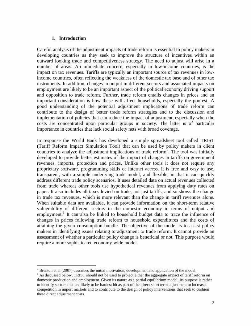
The following figure gives an overview of the structure of TRIST and how it works.
First, the data from customs are organized within the Data Aggregation Tool and then
uploaded into the Simulation Tool within which the user defines the relevant tariff reform
scenarios for each trading partner and parameterizes the elasticities of the trade model
underlying TRIST, which we discuss below. A separate worksheet within the Simulation
Tool presents the results of the chosen reform scenario. It illustrates the impact on tariff,
excise and VAT revenues as well as on prices at the sector level. When available,
production data can be read directly into the Simulation Tool. This additional information
is however not required for TRIST to function.
9 The CPC code allows government, transit and temporary imports to be identified and excluded. These
types of import transactions should be excluded from the analysis as they do not enter the domestic market
and/or are not subject to import duties and other taxes applied at the border. Studies that simply use total
imports inclusive of these official and temporary imports will underestimate the degree of protection in the
economy and overstate the importance of exemptions.
9
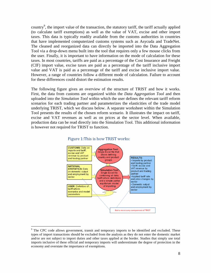
An integral part of TRIST is the trade model that underlies the quantification of the
effects of trade reform scenarios on imports, revenues and production. For each product,
the model first determines the domestic duty and trade tax inclusive import price change
for each trading partner in response to the tariff reform. The trade response to the
resulting percentage price change is then modeled in three consecutive steps. First, the
model allows for the substitution of imports from one trading partner for imports from
another trading partner following changes in relative prices of different suppliers due to
preferential changes in tariffs.10
Second, the model allows for substitution between
imports and domestic production as the relative price of overall imports of the product
changes relative to the price of domestic production. Third, the model allows for a
demand (real income) effect according to which the overall consumption of a product
changes in response to a change in the overall price of the product.
The trade model in TRIST is based on five core assumptions: First, the model is derived
from standard consumer demand theory and utilizes elasticities to determine the
magnitude of the demand response to the price changes that result from a tariff reform.11
Second, the calculations are based on the standard Armington (1969) assumption of
imperfect substitution between imports from different trading partners since consumers
distinguish products by the place of production. This intuitive assumption is standard in
empirical international trade work and implies that a fall in the price of imports from
country A relative to country B will only lead to a partial and not complete substitution of
imports from country B with imports from country A.
Third, the model does not allow for direct substitution between different products. In
other words, each product is modeled as a separate market and in isolation from other
markets. This is perhaps the strongest assumption used in the model. However, a
relaxation would not only complicate computations but would also generate a need for a
range of additional ad-hoc assumptions regarding the precise design of the additional
substitution effect and its parameterization. In the light of our goal to keep the model
simple and transparent and to facilitate country ownership of the tool, we do regard this
simplifying assumption a sacrifice worth making.
Fourth, it is assumed that all changes in tariffs are fully passed on and that the world price
remains unchanged. That is to say that we assume an infinite supply elasticity of imports
10
Note that this substitution between importers will also be relevant for a reduction in MFN tariffs
implemented unilaterally or in the context of multilateral negotiations at the WTO. This is because almost
all countries have one or more free trade partners through bilateral or regional agreements so that even an
MFN reduction will affect the relative price of different imports. 11
Given that the elasticities determine percentage changes in imports, this implies that zero trade flows
remain zero before and after any given reform and there is no market entry of new trading partners. In other
words, if country A does not import sugar cane from country B then no reform can change this fact. The
assumption is a limitation, common to other models, but allows the calculations to remain simple and
manageable. The inaccuracy resulting from the assumption is not likely to be of a large magnitude, yet
should be borne in mind when interpreting the final simulation results. If local knowledge suggests that
there is a potential for substantial new trade this could be handled in the model by allowing for a very small
initial value and a high elasticity.

10
so that changes in demand in the importing country have no effect on the world price of
the product; a realistic assumption for small low income economies.
Fifth, the trade model in TRIST is a partial equilibrium model that treats demand for each
product in isolation from the rest of the economy. Hence, it does not take into account
inter- and intra-sectoral linkages or the economy wide impacts of tariff changes. But this
is not the primary objective of TRIST, which is designed so as to avoid the degree of
aggregation of the data that would be necessary in order to implement economy wide
computable equilibrium models and to remain simple and transparent in its assumptions,
with the flexibility to adjust the key parameters.12
Thus, TRIST has been designed with
the specific task of providing policy makers with important insights into the short-term
effects of trade reform. It has not been designed for making longer-term predictions about
the broad economy wide impact of trade reform.13
By its comparative static nature TRIST
allows the comparison of two states - one in which the base values of policy instruments
(such as tariffs) are unchanged and another in which these base values are exogenously
changed.
Let us now have a closer look at the three calculation steps determining the import
response in our trade model.14
In the first stage we model the allocation of given
expenditure on imports of a product across different country suppliers and how this
allocation changes when tariffs and duties are amended. The exporter substitution effect
defines how imports from exporter A are substituted for imports from exporter B when
the price of imports from exporter A relative to B declines, for example following a
preferential trade reform that includes exporter A but not exporter B. The extent to which
a given change in relative prices translates into a change in relative imports depends on a
user-defined exporter substitution elasticity. In order to isolate the exporter substitution
effect, total imports are held constant in this step.
In the second calculation step, total expenditure on a given product is allocated between
domestic sources and imports. The domestic substitution effect allows for a demand shift
between domestic production and imports when the relative price of imports changes.15
The extent to which the share of imports in domestic consumption changes depends on a
user defined domestic substitution elasticity. The change in imports is then distributed
across all importers according to their share of the import market. This calculation step
can only be modeled if data on domestic production is available.
12
However, the outputs from TRIST in terms of actually applied tariffs and other taxes levied at the border
can be used as an input to improve the accuracy of computable general equilibrium models. 13
For example, TRIST looks only at the import side of the economy whereas trade reform will also have an
impact on exporting sectors by reducing bias against exporting. 14
For detailed formal calculation steps, consult Annex 1. 15
When calculating the impact on employment it is also necessary to make an additional assumption that
there are no second round effects, i.e. that the domestic output-employment ratio does not change in
response to the trade policy change. In practice, over the medium to longer term, tariff reform leads
changes in efficiency that will further influence the impact of employment.
11
Figure 2: The Trade Model
The third and final calculation step allows for an overall demand effect in response to the
change in the average price of domestic consumption of the good. The average price
change is computed as an average of the price change in imports and the price change in
domestic production, weighted by their relative shares in domestic consumption. A
decrease/increase in the average price of the product leads to a percentage
increase/decrease in overall consumption of the product, proportionately distributed
between imports and domestic production. The extent to which imports change for a
given change in the overall price depends on a user-defined import demand elasticity.
This description of the three calculation steps has outlined the crucial role played by
elasticities as the parameters of the model. Elasticities are notoriously difficult to estimate
and so detailed and robust estimates of the three elasticities (exporter substitution,
domestic substitution, demand) are not readily available in the literature. TRIST includes
sensible default values for each of these three parameters that are common across
products and import suppliers. The sensitivity of the results can be easily assessed by
changing the values of the elasticities.
When detailed local knowledge on these elasticities is available, TRIST allows users to
define trading partner and product specific elasticities. Furthermore, there is an option to
include the most well-known estimates of elasticities in the literature. First, the user can
choose to incorporate the import demand elasticities estimated in Kee et al (2004).
However, these elasticities are not available for all product groups (HS 6 digit). Second,
the user can choose to use the product specific import demand elasticities used in
SMART.16
For exporter substitution elasticities or domestic substitution elasticities there
are no estimates available at the level of product detail that TRIST uses.
16
It is good practice to experiment with different sets of elasticities as robustness checks when analyzing
the revenue and production impacts of a trade policy scenario. The default elasticities used in this paper are
1.5 (exporter substitution), 1 (domestic substitution) and 0.5 (demand). Let us illustrate the changes in the
projections when using the Kee et al (2004) and the SMART elasticities. As an example we consider an
EPA between Nigeria and the EU. A once and for all reduction in Nigerian tariffs on EU imports is
projected to lead to a 16.8 percent reduction in overall Nigerian trade tax revenues according to our default

12
4. Examples of Policy Issues that can be Addressed in TRIST
As part of the process of development, countries tend to move towards more open
economies and less reliance on customs duties as a source of revenue. An important issue
in this transition is the short term adjustment costs in terms of fiscal revenue and
domestic production and employment that can arise as low income countries liberalize
their tariff schedules. A lack of knowledge of the likely magnitude of these adjustment
costs can be a factor delaying the implementation of trade reforms. In this section, we
will give some examples of how TRIST can be used to determine the likely size of these
short term adjustment costs. We begin by focusing on the revenue implications and then
move on to show how TRIST can be used to provide useful insights into the potential
short-term impact of tariff reforms on domestic production and employment, poverty and
trade diversion. In the following, we go through some examples of unilateral, bilateral
and regional trade reforms that have been analyzed using TRIST.
4.1. The Core Focus of TRIST: Revenue Impact of Trade Reform
TRIST has to date been developed for a range of countries, including many African countries
and in particular countries participating in regional trade initiatives such as the Economic
Community of Western African States (ECOWAS), the Southern African Development
Community (SADC), the Southern African Customs Union (SACU), the East African
Community (EAC) and the Common Market for Eastern and Southern Africa (COMESA).
We provide a few illustrative trade policy scenarios involving selected countries pertaining to
one or more of these initiatives.
Example 1: The COMESA Customs Union. A pressing trade policy issue currently facing
COMESA members is the impact of joining the customs union (CU). It is interesting to
analyze what a customs union would imply for the revenue situation of different
COMESA members. We choose three countries to analyze the impact of such a scenario,
Malawi, Kenya and Zambia. The trade policy scenario is defined as follows: all the
remaining non-zero intra-COMESA tariffs are set to zero. This implies assuming that a
complete COMESA Free Trade Agreement (FTA) is put in place before the
implementation of the customs union. Preferential tariffs with SADC members remain
the same. The COMESA Common External Tariff (CET)17
is applied to all remaining
trading partners. However, in order to account for tariff exemptions, statutory tariffs in
the CET schedule are multiplied by the current ratio of collection efficiency, i.e. the tariff
revenue that has been collected divided by the revenue that should have been collected
according to the current statutory rates.18
elasticities, a 14.6 percent reduction when using the Kee et al (2004) estimated demand elasticities and a
14.3 percent reduction when using the SMART elasticities. 17
We use the COMESA CET schedule as of 24.10.2008. 18
To date, TRIST can only model tariff changes in a single importing market, whereas several importing
markets simultaneously change when CETs are adjusted. We are currently working on extending TRIST in
this respect.

13
Table 2: Revenue Implications of a COMESA Common External Tariff
in millions of USD
Country
Elasticities default high default high default high
Old imports 1416.0 1416.0 3930.9 3930.9 9909.1 9909.1
New Import 1416.6 1419.0 3949.5 3972.5 9947.9 9965.6
Change 0.6 2.9 18.6 41.7 38.9 56.5
% Change 0.0% 0.2% 0.5% 1.1% 0.4% 0.6%
Old tariff revenue 75.9 75.9 245.8 245.8 436.4 436.4
New tariff revenue 72.2 69.3 203.0 196.0 330.3 319.1
Change -3.6 -6.6 -42.8 -49.8 -106.2 -117.3
% Change -4.8% -8.7% -17.4% -20.3% -24.3% -26.9%
Old excise revenue 78.8 78.8 98.5 98.5 517.6 517.6
New excise revenue 78.4 79.0 98.0 98.5 517.6 517.6
Change -0.4 0.1 -0.5 -0.1 0.0 0.0
% Change -0.6% 0.2% -0.5% -0.1% 0.0% 0.0%
Old VAT revenue 117.0 117.0 684.7 684.7 798.4 798.4
New VAT revenue 115.9 116.9 680.1 683.5 794.2 796.3
Change -1.2 -0.1 -4.5 -1.1 -4.1 -2.0
% Change -1.0% -0.1% -0.7% -0.2% -0.5% -0.3%
Old total revenue 271.8 271.8 1029.0 1029.0 1752.4 1752.4
New total revenue 266.5 265.2 981.2 977.9 1642.1 1633.0
Change -5.2 -6.6 -47.8 -51.0 -110.3 -119.3
% Change -1.9% -2.4% -4.6% -5.0% -6.3% -6.8%
Old collected tariff rate 5.4% 5.4% 6.3% 6.3% 4.4% 4.4%
New collected tariff rate 5.1% 4.9% 5.1% 4.9% 3.3% 3.2%
1) The COMESA CET scenario assumes zero tariffs among COMESA partners, unchanged tariffs for SADC partners. For all other trading partners,
the new CET rate is applied but deflated by the current ratio of collection efficiency (collected tariff rate / statutory tariff rate) to account for tariff
exemptions. In the few cases of tariff lines for which no final agreement has been reached yet the lowest tariff rate under consideration is used.
2) The default scenario assumes 0.5 for import demand elasticity, 1.5 for exporter substitution elasticity. High scenario assumes 1 for import
demand elasiticity, 5 for exporter subsitution elasticity.
Malawi Zambia Kenya
Table 2 presents results of revenue losses from the above defined COMESA CET
scenario. We choose two sets of elasticity values: the standard default values and higher
values to assess sensitivity.19
In Malawi, the implementation of the CET is projected to
19
Default (high) choices for elasticities: Exporter Substitution Elasticity: 1.5 (5), Demand Elasticity: 0.5 (1)

14
lead to a moderate reduction in protection as the import weighted average tariff rate falls
from 5.4 to 5.1 percent. Tariff revenues are projected to fall by US$ 3.6 million with the
default elasticities and by US$6.6 million with the higher elasticity values corresponding
to losses of between 4.8 and 8.7 percent. Tariff reductions affect excise and VAT
revenues in two ways: first, there is an increase in imports that drives up other trade tax
revenues along with tariffs. Second, the reduction in tariffs lowers the tax base for excise
taxes and VAT in most countries, including Malawi.20
Total trade revenue losses from
tariffs, excises and VAT are projected to be between US$ 5.2 and 6.6 million, a fall of
about 2 to 2.5 percent in overall trade tax revenues.
Zambia and Kenya would lose proportionately more revenue as a result of the
implementation of the CET schedule since the decline in protection from implementing
the CET would be larger than in Malawi. The tariff revenue loss is predicted to be
between 17 and 20% in Zambia and between 24 and 27% in Kenya. The total trade
revenue loss is projected as being between 4.6 and 5% in Zambia and between 6.3 and
6.8% in Kenya.
Example 2: An Economic Partnership Agreement with the EU. An important challenge
for many low income countries is the negotiation and implementation of EPAs with the
EU. In contrast to the previous Cotonou and Lome Agreements, these new agreements
call for the reciprocal elimination of tariffs on imports from the EU. In many African,
Caribbean and Pacific countries lack of information about the potential magnitude of the
adjustment costs that will arise from removing tariffs against imports from the EU has led
to considerable uncertainty and apprehension concerning these agreements.21
20
A higher demand elasticity will accentuate the impact of tariff reductions on the level of overall imports
and therefore the positive impact on VAT and excise revenues. 21
There are many studies in the literature that have attempted to estimate the revenue implications of EPA
agreements between the European Union and various African countries. These include Brenton et al
(2007), Busse and Grossmann (2004), Karingi et al (2005), Khandelwal (2004) and Milner et al (2005) to
name a few. Brenton et al (2007) discuss the relative merits of the methodologies used.
15
Table 3: Revenue Implications of an Economic Partnership Agreement (EPA) with the European Union
in millions of USD
Country Tanzania Kenya Ethiopia
EPA Sensitive list exemptions cut EPA Sensitive list exemptions cut EPA Sensitive list exemptions cut
Old imports 5802.8 5802.8 5802.8 10057.5 10057.5 10057.5 3589.7 3589.7 3589.7
New Import 5819.4 5805.5 5770.2 10093.3 10057.7 9984.0 3610.9 3589.8 3576.5
Change 16.6 2.7 -32.7 35.8 0.2 -73.5 21.2 0.2 -13.2
% Change 0.3% 0.0% -0.6% 0.4% 0.1% -0.7% 0.6% 0.0% -0.4%
Old tariff revenue 270.3 270.3 270.3 443.0 443.0 443.0 291.7 291.7 291.7
New tariff revenue 231.4 264.7 318.6 357.2 420.3 537.8 241.8 275.6 305.6
Change -38.9 -5.7 48.2 -85.7 -22.6 94.8 -49.9 -16.0 13.9
% Change -14.4% -2.2% 17.8% -19.4% -5.7% 21.4% -17.1% -5.5% 4.8%
Old excise revenue 294.4 294.4 294.4 525.3 525.3 525.3 68.9 68.9 68.9
New excise revenue 294.0 294.4 294.3 524.2 525.3 525.2 70.1 68.9 70.0
Change -0.4 0.0 -0.1 -1.1 -0.1 -0.1 1.2 0.0 1.1
% Change -0.1% 0.0% 0.0% -0.2% 0.0% 0.0% 1.7% 0.0% 1.6%
Old VAT revenue 528.5 528.5 528.5 810.3 810.3 810.3 297.1 297.1 297.1
New VAT revenue 525.3 528.3 528.6 803.7 809.1 803.4 293.8 296.3 295.5
Change -3.2 -0.1 0.1 -6.6 -1.2 -6.9 -3.2 -0.8 -1.5
% Change -0.6% 0.0% 0.0% -0.8% -0.2% -0.9% -1.1% -0.3% -0.5%
Old total revenue 1093.2 1093.2 1093.2 1778.6 1778.6 1778.6 657.7 657.7 657.7
New total revenue 1050.8 1087.4 1141.4 1685.1 1754.7 1866.4 605.7 640.8 671.1
Change -42.4 -5.8 48.2 -93.5 -23.9 87.8 -52.0 -16.8 13.4
% Change -3.9% -0.5% 4.4% -5.3% -1.5% 4.9% -7.9% -2.6% 2.0%
Old collected tariff rate 4.7% 4.7% 4.7% 4.4% 4.4% 4.4% 8.1% 8.1% 8.1%
New collected tariff rate 4.0% 4.6% 5.5% 3.5% 4.2% 5.4% 6.7% 7.8% 8.5%
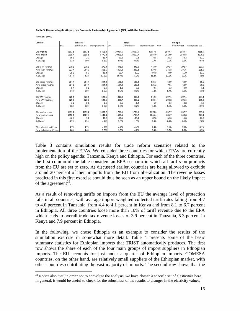
Table 3 contains simulation results for trade reform scenarios related to the
implementation of the EPAs. We consider three countries for which EPAs are currently
high on the policy agenda: Tanzania, Kenya and Ethiopia. For each of the three countries,
the first column of the table considers an EPA scenario in which all tariffs on products
from the EU are set to zero. As discussed earlier, countries are being allowed to exclude
around 20 percent of their imports from the EU from liberalization. The revenue losses
predicted in this first exercise should thus be seen as an upper bound on the likely impact
of the agreement22
.
As a result of removing tariffs on imports from the EU the average level of protection
falls in all countries, with average import weighted collected tariff rates falling from 4.7
to 4.0 percent in Tanzania, from 4.4 to 4.1 percent in Kenya and from 8.1 to 6.7 percent
in Ethiopia. All three countries loose more than 10% of tariff revenue due to the EPA
which leads to overall trade tax revenue losses of 3.9 percent in Tanzania, 5.3 percent in
Kenya and 7.9 percent in Ethiopia.
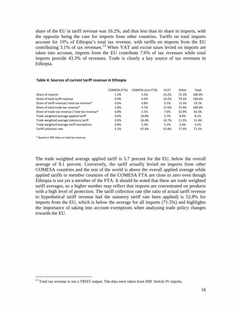
In the following, we chose Ethiopia as an example to consider the results of the
simulation exercise in somewhat more detail. Table 4 presents some of the basic
summary statistics for Ethiopian imports that TRIST automatically produces. The first
row shows the share of each of the four main groups of import suppliers in Ethiopian
imports. The EU accounts for just under a quarter of Ethiopian imports. COMESA
countries, on the other hand, are relatively small suppliers of the Ethiopian market, with
other countries contributing the vast majority of imports. The second row shows that the
22
Notice also that, in order not to convolute the analysis, we have chosen a specific set of elasticities here.
In general, it would be useful to check for the robustness of the results to changes in the elasticity values.
16
share of the EU in tariff revenue was 16.2%, and thus less than its share in imports, with
the opposite being the case for imports from other countries. Tariffs on total imports
account for 19% of Ethiopia‟s total tax revenue, with tariffs on imports from the EU
contributing 3.1% of tax revenues.23
When VAT and excise taxes levied on imports are
taken into account, imports from the EU contribute 7.6% of tax revenues while total
imports provide 43.3% of revenues. Trade is clearly a key source of tax revenues in
Ethiopia.
Table 4: Sources of current tariff revenue in Ethiopia
COMESA (FTA) COMESA (non-FTA) EU27 Other Total
Share of imports 1.2% 3.2% 23.2% 72.3% 100.0%
Share of total tariff revenue 0.0% 4.3% 16.2% 79.5% 100.0%
Share of tariff revenue/ total tax revenue* 0.0% 0.8% 3.1% 15.3% 19.2%
Share of total trade tax revenue* 1.8% 4.7% 17.6% 75.9% 100.0%
Share of trade tax revenue / total tax revenue* 0.8% 2.1% 7.6% 32.9% 43.3%
Trade weighted average applied tariff 0.0% 10.8% 5.7% 8.9% 8.1%
Trade weighted average statutory tariff 0.9% 16.0% 10.7% 11.5% 11.4%
Trade weighted average tariff exemptions 0.8% 5.2% 5.1% 2.6% 3.2%
Tariff collection rate 5.1% 67.6% 52.8% 77.4% 71.5%
* Based on IMF data on total tax revenue
The trade weighted average applied tariff is 5.7 percent for the EU, below the overall
average of 8.1 percent. Conversely, the tariff actually levied on imports from other
COMESA countries and the rest of the world is above the overall applied average while
applied tariffs to member countries of the COMESA FTA are close to zero even though
Ethiopia is not yet a member of the FTA. It should be noted that these are trade weighted
tariff averages, so a higher number may reflect that imports are concentrated on products
with a high level of protection. The tariff collection rate (the ratio of actual tariff revenue
to hypothetical tariff revenue had the statutory tariff rate been applied) is 52.8% for
imports from the EU, which is below the average for all imports (71.5%) and highlights
the importance of taking into account exemptions when analyzing trade policy changes
towards the EU.
23
Total tax revenue is not a TRIST output. The data were taken from IMF Article IV reports.
17
hscode Product
72142000 IRON/STEEL BARS & RODS,HOTROLLED,TWISTED/WITH DEFORMTNS …….
87032210 VEHICLES WITH SPARK-IGNITION ENGINE OF CYL.CAPC 1000<C_C<1300CC
87089900 PARTS AND ACCESSORIES, NES, FOR VEHICLES OF 87.01 TO 87.05
24022000 CIGARETTES CONTAINING TOBACCO
87021010 PUB. TRANSPORT TYPE VEHICLE(DIESLE/SEMI-D) SEAT CAPACITY < 15 PASS.
87033390 VEHICLES WITH DIESEL/SEMI-D ENGINE CYLINDER CAPACITY > 2500CC, NES
87042109 GOODS VEHICLE WITH DIS/SEMI-DENGINES, GVW <= 5 TONNE ……..
30043900 MEDICAMENTS OF OTHER HORMONES, FOR RETAIL SALE, NES
19019090 OTHER FOOD PREPARATIONS OF FLOUR ETC,NES
87032390 VEHICLES WITH SPARK IGNITION ENGINE OF CYLINDER CAPACITY >1800CC…
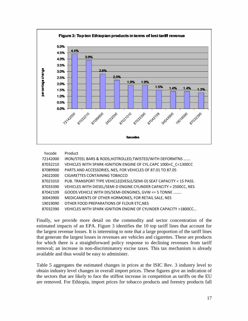
Finally, we provide more detail on the commodity and sector concentration of the
estimated impacts of an EPA. Figure 3 identifies the 10 top tariff lines that account for
the largest revenue losses. It is interesting to note that a large proportion of the tariff lines
that generate the largest losses in revenues are vehicles and cigarettes. These are products
for which there is a straightforward policy response to declining revenues from tariff
removal; an increase in non-discriminatory excise taxes. This tax mechanism is already
available and thus would be easy to administer.
Table 5 aggregates the estimated changes in prices at the ISIC Rev. 3 industry level to
obtain industry level changes in overall import prices. These figures give an indication of
the sectors that are likely to face the stiffest increase in competition as tariffs on the EU
are removed. For Ethiopia, import prices for tobacco products and forestry products fall

18
by around 15%. For all other sectors the competition effect is likely to be milder with
price changes of imports of less than 5 percent.
The nature of competition in the import market is a critical determinant of who benefits
from the tariff reductions under an EPA. If competition is limited, then it is possible that
EU firms will capture the rents created when tariffs against the EU are removed, import
prices in Ethiopia may decline by less than the fall in the duty and there will be a transfer
of some or all of the previously collected tariff revenue to EU firms with little or no
beneficial impact on the domestic market. This is a key reason why MFN liberalization
should accompany preferential tariff reductions.
Table 5: Ethiopian import price changes by sector under EPA scenario
ISIC Rev. 3 industry Import weighted average price change Share in total imports
16 - Manufacture of tobacco products -15.9% 0.1%
02 - Forestry, logging and related service activities -14.9% 0.1%
13 - Mining of metal ores -4.4% 0.0%
26 - Manufacture of other non-metallic mineral products -3.3% 1.0%
34 - Manufacture of motor vehicles, trailers and semi trailers -2.8% 6.8%
…
18 - Manufacture of wearing apparel; dressing and dyaing of fur -0.0% 1.9%
01 - Agriculture, hunting and related service activities -0.0% 7.8%
11 - Extraction of crude petroleum and natural gas … -0.0% 0.4%
23 - Manufacture of coke, refined petroleum products and nuclear fuel -0.0% 16.2%
40 - Electricity, gas, steam and hot water supply -0.0% 0.0%
As mentioned previously revenue losses projected here and in Table 3 are upper bounds
on the likely impact of the EPAs with the EU. Countries can negotiate to exclude some
20% of their imports from the EU from the agreement, meaning that tariffs on these
products can be left unchanged. There are several ways that countries may choose the
products to be excluded from the agreement. The reality is that many countries simply
choose those products that have the highest levels of protection. In TRIST any user-
defined list of products can be selected to be excluded from the EPA or any other trade
agreement since the model is based on data at the tariff line level. As an example, we
look at the case in which countries choose the exclusion list to minimize the adverse
revenue impact on the agreement. In TRIST we can simply run the EPA scenario without
an exclusion list and rank products by the ratio of overall trade tax revenue loss to import
value. We then include the most revenue sensitive products, accounting for just less than
20% of trade with the EU, on the exclusion list.
The results from this scenario are presented in the second column of Table 3 for each of
the three countries and show that the fall in tariff revenues compared to the initial EPA
scenario without the exclusion list is considerably reduced by between 12 and 14
percentage points for the three countries. The overall trade tax losses under this scenario
amount to 0.5% (Tanzania), 1.3% (Kenya) and 2.6% (Ethiopia). For some countries
official exclusion lists for a potential EPA have already been determined. Among these
are the EAC member states Tanzania and Kenya. Table 6 contrasts the impact of an EPA
under the revenue loss minimizing scenario outlined column two of Table 3 with a
scenario in which the official EAC exclusion list is used. In the case of Tanzania the

19
projected 1.5% loss in trade tax revenue is only slightly higher than the losses projected
for the revenue loss minimization case, whereas revenue losses for Kenya are closer to
the projected impact for an EPA without an exclusion list. This indicates that the EAC
exclusion list may have been determined to respond more closely to Tanzanian rather
than Kenyan revenue concerns.
Table 6A: Tanzanian EPA with Official EAC Exclusion List
EPA with 80% Sensitive List EPA with Official EAC Exclusion List
Total Number of Tariff Lines 4,393 4,393
Number of Excluded Product Lines 1,581 1078*
% Change in Imports 0.0% 0.1%
% Change in Tariff Revenue -2.2% -6.4%
% Change in Total Revenue -0.5% -1.7%
Old Collected Tariff Rate 4.70% 4.70%
New Collected Tariff Rate 4.60% 4.40%
*In total there are 1,390 lines on the Official EAC Exclusion List. However, only 1,078 lines are suject to imports to Tanzania in 2008.
Table 6B: Kenyan EPA with Official Exclusion List
EPA with 80% Sensitive List EPA with Official EAC Exclusion List
Total Number of Tariff Lines 4,363 4,363
Number of Excluded Product Lines 1,597 1075*
% Change in Imports 0.1% 0.3%
% Change in Tariff Revenue -5.7% -17.8%
% Change in Total Revenue -1.5% -4.8%
Old Collected Tariff Rate 4.4% 4.4%
New Collected Tariff Rate 4.2% 3.6%
*In total there are 1,390 lines on the Official EAC Exclusion List. However, only 1,075 lines are suject to imports to Tanzania in 2008.
Another policy response to declining tariff revenues due to trade liberalization that can
easily be assessed in TRIST is the removal of tariff exemptions. Tariff exemptions for
certain importers or certain products are distortive and often are not based upon clear and
transparent decisions relating to a competitiveness strategy. Hence, cutting exemptions
can be useful to offset projected revenue reductions emanating from trade liberalization.
In order to illustrate the magnitude of the gain in revenue that can be achieved we
consider the following scenario: as part of the EPA, all tariffs with the EU are set to zero
and there is no exclusion list. Statutory tariffs with all other trading partner are left as
they are but tariff exemptions are cut to zero. In Table 3 the third column presents the
impact of this policy reform scenario for all trading partners. The results show that all
three countries gain substantial amounts of tariff and overall trade tax revenue by cutting
exemptions despite the fact that all tariffs with the EU are set to zero. Similarly, in all
three countries the reform actually leads to an increase (of between 2 and 4 percent)
rather than a decrease in import weighted average collected tariffs.

20
However, the removal of tariff exemptions could exacerbate the negative, trade diverting,
impact of the preferential trade agreement. It is important that a country also seek to
reduce its MFN tariffs to reduce the possible distortion that arise from removing tariffs
against particular suppliers and not others. Hence, the removal of tariff exemptions as
tariffs against the EU are removed should be integrated into a policy to reduce external
tariffs. For example, removing all tariff exemptions would allow Tanzania to cut its MFN
tariffs by more than 30% at the same time as implementing the EPA agreement without
any adverse revenue impact. Similarly, Ethiopia could cut its MFN tariffs by more than
20% and Kenya by more than 40%.
Example 3: The Impact of Specific and Complex Duties. Another advantage of TRIST is
that it can deal more effectively with specific and complex tariffs than can models based
on statutory rates. Specific tariffs are those in which the duty is related to the volume or
other physical characteristics of the product while complex tariffs combine different
types of duty such as ad valorem and specific tariffs. A key feature of specific and
complex tariffs is that the level of protection given by the statutory rate is not transparent
and in practice will vary across different transactions of the same product. These tariffs
are a particularly pernicious source of revenue, with ad-valorem equivalent rates often by
far exceeding 100%. More specifically these tariffs tend to be regressive with higher
levels of protection on the lower value transactions that are consumed by poor
households. While specific taxes avoid the issue of valuation of an import transaction
they can allow for discretion and corruption and substantially increase collection costs at
customs when all transactions subject to these duties require physical inspection.
Table 7: Specific Tariffs in Tanzania
Product Tariff
Rice in the husk (paddy or rough) 75% or USD 200/MT whichever is higher
Husked (brown) rice 75% or USD 200/MT whichever is higher
Semimilled or wholly milled rice … 75% or USD 200/MT whichever is higher
Broken rice 75% or USD 200/MT whichever is higher
Cane sugar 100 % or USD 200/MT whichever is higher
Of jute or of other textile bast fibres of heading 45% or USD 0.45/bag whichever is higher
Worn clothing and other worn articles 45% or USD 0.30/kg whichever is higher
The data in TRIST is based on actual revenues collected and so TRIST automatically
computes ad-valorem equivalents of specific and complex tariffs for each product by
country import flow. Other models typically use some average ad valorem equivalent that
aggregates away the complexity of these duties. Hence, TRIST can show the revenue and
other adjustment implications of removing specific and complex tariffs or of strategies to
convert them into ad valorem rates. This may be important information in defining the
time period over which such a reform is implemented. Other models are unable to
accurately assess the revenue impact of removing these duties.

21
-9.0%
-8.0%
-7.0%
-6.0%
-5.0%
-4.0%
-3.0%
-2.0%
-1.0%
0.0%
cap at 25% cap at 15% cap at 10% all zero
Figure 4: Reform of special tariffs: cutting ad-valorem equivalents
Change in Tariff Revenue
Change in Trade Tax Revenue
Table 7 shows statutory complex tariffs in the Tanzanian tariff schedule and Figure 4
illustrates the revenue implications of converting them to ad-valorem equivalents and
subsequently capping these. As is common, the specific and complex tariffs are not
important sources of revenue and their revenue impact is small relative to the costs a
country incurs in terms of economic distortions and administrative costs at customs when
maintaining them.
Finally, notice that TRIST allows analysis of the impact of sequencing the different
elements of a trade reform. An interesting example is presented in the next section in the
context of the analysis of trade diversion.
4.2. Extensions of TRIST
Up to this point, this paper has focused on the analysis of revenue changes in response to
trade policy reforms. Yet, revenue effects are not the only adjustment cost policymakers
may need to address. The following analysis shows how TRIST can be extended to
provide input to an analysis of the impact of trade reforms on domestic production and
employment, poverty as well as on trade diversion. It is straightforward to adapt TRIST
to contribute to these additional and crucially policy relevant topics.
However, again, it is important to note that TRIST uses a partial equilibrium model and
thus does not take into account inter- and intra-sectoral linkages and the economy wide
impacts of tariff changes. The results presented below are based on tariff-line level partial
equilibrium simulations which do not take into account the various economy-wide
resource constraints and reallocations, or any inter- and intra-sectoral economic linkages
that may be important for the medium to long term impacts of the respective reforms. 24
24
The equilibrium allocation of resources is much less important when there is a large amount of
unemployed or underemployed resources, especially labor.
22
One of the core benefits of trade liberalization is that it removes the anti export bias in
economies with high levels of protection which will depreciate the real exchange rate and
allow export sectors to compete more effectively for domestic factors of production. This
not only implies that export intensive sectors might benefit disproportionately from trade
liberalization and are likely to expand in the medium to long term, but also that an
assessment of the short-term aggregate impact of a liberalization scenario may be subject
to a systematic upward bias.25
These concerns are less of an issue with respect to relative sectoral impacts of tariff
reform. Given its nature as a partial equilibrium model, the purpose of TRIST in
contributing to the analysis of trade reform adjustment costs in terms of output and
employment is thus to identify sectors that are likely to be hardest hit as part of the direct
short term adjustment to increased competition in import markets and to contribute to the
design of policy interventions that seek to cushion these direct adjustment costs.26
Production and employment
The impact of trade reforms on domestic production and in particular employment has
been one of the most politically sensitive issues in the discussion on adjustment costs.
The desired long run result of trade liberalization is the reallocation of production factors
(labor and capital) to more productive uses, thus involving changes in the pattern of
production and employment among and within firms, industries and regions. In the short
run, however, production in import competing sectors will likely decline, which may
have social and political costs. A better understanding of these effects is central to
effective sector- and region-specific trade policy making that mitigates these adjustment
costs.
TRIST gives an indication of those sectors that are likely to be most affected by short
term adjustment costs to tariff reform by presenting changes in prices for each sector.
Those sectors facing the largest decline in prices are those that will tend to face the
biggest adjustment. However, this analysis can be considerably enhanced and deepened if
there are detailed sectoral production and employment data. Production and employment
data27
can be uploaded into the simulation tool and TRIST will automatically amend the
model to include the domestic substitution effect as well as present sectoral changes in
domestic production and employment that result from the trade policy scenario of
interest.
25
Although the export impact is likely to not happen in the short run and to be delayed relative to the
import impact of a tariff reduction, the real exchange rate impact of a given reform may happen very soon
in countries that face serious foreign exchange constraints, thus limiting the negative impact on import
competing sectors in the absence of (foreign exchange depletion -) offsetting export expansion. 26
Another reason why TRIST cannot be used to assess the aggregate impact of trade reform on output and
employment is that the data typically are available for industry only and exclude output and employment in
agriculture and services - by far the biggest sources of employment in most developing countries. 27
As only goods that remain in the domestic market compete with imports, it is necessary to delete exports
from the value of domestic production and to only include domestic production exclusive of exports in the
model. A detailed explanation of the necessary steps is available upon request.

23
A country for which a TRIST has been developed and for which the necessary data on
sectoral domestic production are available is Mauritius. Table 8 presents selected results
illustrating the impact of a duty-free island trade policy scenario on domestic production
and employment.28
The table presents changes in domestic production and employment
in the 15 sectors that are projected to be most severely affected (in terms of absolute
production losses) by the reform scenario. The sectors most severely affected are the
manufacture of furniture, the manufacture of wearing apparel, the manufacture of soap
and detergents, the manufacture of bakery products, the manufacture of preserving of
fruits and vegetables and the manufacture of wines.
The overall impact of the scenario on domestic production is rather weak (692 million
Mauritian rupees, which accounts for about 1% of total industrial production). The reason
is that tariff levels are already very low in Mauritius such that substitution effects
resulting from any liberalization scenario are not likely to be large.29
Table 8 also
contains figures illustrating the impact of the trade reform on domestic employment
where the loss accounts for about 2% of total industrial employment30
.
Table 8: Duty-Free Island in Mauritius: 15 most affected sectors
Sector Employment
Change % Change Change
3610 - Manufacture of furniture -115.0 -3.9% -427
1810 - Manufacture of wearing apparel... -111.3 -2.0% -842
2424 - Manufacture of soap and detergents… -58.0 -6.6% -64
1541 - Manufacture of bakery products -53.4 -3.2% -92
1513 - Processing and preserving of fruit and vegetables -31.8 -3.3% -20
1552 - Manufacture of wines -29.8 -6.2% -20
2710 - Manufacture of basic iron and steel -25.2 -1.5% -7
1554 - Manufacture of soft drinks… -23.6 -1.1% -29
2520 - Manufacture of plastics products -21.3 -1.4% -26
1511 - Production, processing and preserving of meat… -21.1 -0.5% -7
3230 - Manufacture of television and radio receivers… -14.9 -3.4% -6
2511 - Manufacture of rubber tyres and tubes… -14.0 -9.5% -23
2109 - Manufacture of other articles of paper… -13.6 -1.9% -19
1920 - Manufacture of footwear -13.3 -7.9% -30
1543 - Manufacture of cocoa, chocolate and sugar confectionery -12.0 -6.9% -7
Output (in Mio Mauritian Rupees)
Poverty
Another interesting extension of TRIST is the analysis of the impact of trade policy
reforms on poverty. Given that TRIST automatically produces results on sectoral price
changes in response to policy reform, it is straightforward to extend the projections to
give an indication of how different population groupings will be affected by these price
changes. An essential requirement for such an analysis is, of course, the availability of a
28
The scenario involves that all tariffs are set to zero. We use an exporter substitution elasticity of 1.5, a
demand elasticity of 0.5 and a domestic substitution elasticity of 1. 29
See also World Bank (2006). 30
These are computed under the assumption that productivity does not change.

24
comprehensive survey distinguishing the consumption patterns of different income
groups. If the necessary data is available, it is possible to use an additional excel file that
has been developed for TRIST to do the analysis. The tool calculates the changes in
consumer expenditure across groupings in response to a given trade reform assuming that
consumption patterns do not change. It is once again important to notice that this analysis
provides only a short-term and a partial view on the issue. There are important economy
wide effects of trade reform that the tool cannot take into account.
We again consider the duty free island scenario for Mauritius for which a comprehensive
consumer expenditure survey is available. Table 9 shows how different income groups
are affected by the reform. The resulting falls in consumer expenditure for different
income groups and for constant consumption baskets range between -1.0 and -1.5
percent. Given that Mauritian tariffs are already very low to start with, it is not surprising
that the reform does not produce larger expenditure changes on average. It is, however,
interesting that changes in expenditure differ between income groups although we
consider a reform that drives tariffs to zero across all product groups. This further
emphasizes the importance of differentiating carefully between different population
groupings when analyzing the impact of trade reforms. In conjunction with the
techniques outlined above to analyze the impact of trade reforms on sectoral employment
and production, the researcher can draw an informative picture of how different
population groups, rather than solely the country as a whole, are affected by the reforms
in the short-term.31
These analyses can form part of a more extensive investigation of the
welfare and poverty impact of trade reform.
Table 9: Expenditure changes in response to tariff reform to duty free island in Mauritius
Income Groups Old Expenditure New Expenditure % Change in Expenditure
All Classes 9568 9442 -1.3%
Less than 2,000 2780 2752 -1.0%
2,000 to <5,000 3598 3556 -1.2%
5,000 to <7,500 5443 5374 -1.3%
7,500 to <10,000 6967 6877 -1.3%
10,000 to <15,000 8941 8819 -1.4%
15,000 to <20,000 11772 11617 -1.3%
20,000 to <30,000 14911 14694 -1.5%
30,000+ 22202 21932 -1.2%
1) In Mauritian Rupees
2) All tariffs are driven to zero
3) Elasticities: Exporter Substitution (1.5), Domestic Substitution (1.5), Demand (0.5)
Trade diversion
A preferential liberalization will reduce prices and increase imports from the beneficiary
country. But at the same time it will displace imports from other (potentially more
efficient) sources. Thus, a preferential liberalization affects not only the overall price
level of the goods affected but also the relative price of goods from different sources.
31
Given that we have information on employment shares across income groups in different sectors.

25
There will be a change in the aggregated level of spending on the goods affected as well
as changes in the composition of the sourcing of these goods. Thus, there is a potential
source of trade diversion.
It is straightforward to determine the amount of imports from trading partner B that is
replaced by imports from trading partner A in response to a preferential trade reform.
However, trade diversion by definition refers to a (welfare decreasing) substitution of
imports from a more efficient source to a less efficient source because of a preferential
reduction in tariffs. Trade diversion thus occurs, for example, if the EU gets duty free
access to the US market and only thereby can sell its products at a lower price than other
more efficient exporters who are not granted the same preferences. Yet, there are also
situations in which diverted trade cannot be classified as trade diversion. Consider the
following example: after the EU is granted tariff free market access it takes over some of
the market share that was previously held by other trading partners who already enjoyed
tariff free market access prior to the EU being granted the tariff reduction. This would not
be trade diversion as it would actually reflect a move of consumption towards a more
efficient producer that was previously disadvantaged in terms of market access. In order
to fix language, we use the term trade correction for this phenomenon.
In order to accurately assess the adverse impact of preferential trade agreements relative
to, say, a reduction in MFN tariffs it is important to take into account this distinction. For
TRIST, an additional Excel file has been developed that sources information from the
simulation tool and calculates estimates of trade diversion volumes that are amended for
„trade correction‟. The tool uses a simple and intuitive methodology. A detailed
explanation is available upon request.
As a practical example, we consider a sequential scenario: we assume that Nigeria has
liberalized all tariffs on imports from the EU to zero as part of an EPA. The resulting
import allocations and tariff rates are taken as the „base scenario‟ for the following policy
experiment, namely an FTA between Nigeria and China. Table 10 shows how different
trading partners would be affected in terms of their exports to Nigeria if Nigerian tariffs
on all Chinese imports were preferentially driven to zero as part of the FTA. The table
distinguishes two categories of diverted trade as outlined above: diverted trade can be
either welfare reducing (trade diversion) or it can happen in response to a decrease in
preferences previously granted which is not welfare reducing (trade correction).
26
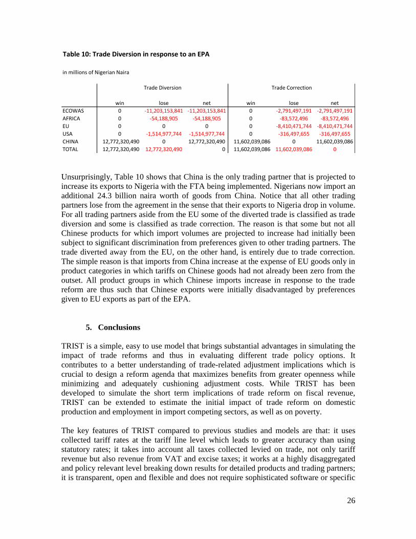
Table 10: Trade Diversion in response to an EPA
in millions of Nigerian Naira
win lose net win lose net
ECOWAS 0 -11,203,153,841 -11,203,153,841 0 -2,791,497,191 -2,791,497,191
AFRICA 0 -54,188,905 -54,188,905 0 -83,572,496 -83,572,496
EU 0 0 0 0 -8,410,471,744 -8,410,471,744
USA 0 -1,514,977,744 -1,514,977,744 0 -316,497,655 -316,497,655
CHINA 12,772,320,490 0 12,772,320,490 11,602,039,086 0 11,602,039,086
TOTAL 12,772,320,490 12,772,320,490 0 11,602,039,086 11,602,039,086 0
Trade Diversion Trade Correction
Unsurprisingly, Table 10 shows that China is the only trading partner that is projected to
increase its exports to Nigeria with the FTA being implemented. Nigerians now import an
additional 24.3 billion naira worth of goods from China. Notice that all other trading
partners lose from the agreement in the sense that their exports to Nigeria drop in volume.
For all trading partners aside from the EU some of the diverted trade is classified as trade
diversion and some is classified as trade correction. The reason is that some but not all
Chinese products for which import volumes are projected to increase had initially been
subject to significant discrimination from preferences given to other trading partners. The
trade diverted away from the EU, on the other hand, is entirely due to trade correction.
The simple reason is that imports from China increase at the expense of EU goods only in
product categories in which tariffs on Chinese goods had not already been zero from the
outset. All product groups in which Chinese imports increase in response to the trade
reform are thus such that Chinese exports were initially disadvantaged by preferences
given to EU exports as part of the EPA.
5. Conclusions
TRIST is a simple, easy to use model that brings substantial advantages in simulating the
impact of trade reforms and thus in evaluating different trade policy options. It
contributes to a better understanding of trade-related adjustment implications which is
crucial to design a reform agenda that maximizes benefits from greater openness while
minimizing and adequately cushioning adjustment costs. While TRIST has been
developed to simulate the short term implications of trade reform on fiscal revenue,
TRIST can be extended to estimate the initial impact of trade reform on domestic
production and employment in import competing sectors, as well as on poverty.
The key features of TRIST compared to previous studies and models are that: it uses
collected tariff rates at the tariff line level which leads to greater accuracy than using
statutory rates; it takes into account all taxes collected levied on trade, not only tariff
revenue but also revenue from VAT and excise taxes; it works at a highly disaggregated
and policy relevant level breaking down results for detailed products and trading partners;
it is transparent, open and flexible and does not require sophisticated software or specific
27
programming skills. The overarching goal of TRIST is to provide a tool to government
agencies and other stakeholders that can use it to support an informed discussion of the
possible short-term consequences of tariff reforms.
It is hoped that free access to the spreadsheet tool will allow researchers and government
officials to fine tune TRIST to reflect country circumstances, and will enable them to
analyze the impact of proposals for trade policy reform as they arise. An aim of this paper
and tool is also to encourage the collection of more accurate and detailed data on
production, employment and consumption. This is important to allow for more systematic
analysis of the impact of trade (and other) policy changes on output, employment,
consumption and poverty so as to help motivate positive interventions that limit the
adjustment costs, and so maximize the overall positive economic benefits, of trade
reform.
TRIST templates as well as a TRIST manual and additional information are available on
the TRIST website under http://go.worldbank.org/2P8FPC0760.
28
Bibliography
Andriamananjara, S., P. Brenton, E. von Uexkull and P. Walkenhorst (2009),”Assessing
the Economic Impacts of an Economic Partnership Agreement on Nigeria”, World Bank
Policy Research Working Paper 4920.
Armington, P. (1969), “A Theory of Demand for Products Distinguished by Place of
Production,” IMF Staff Papers, 16, pp. 159-178.
Brenton, P., M. Hoppe, E. v. Uexkull (2007), “Evaluating the Revenue Effects of Trade
Policy Options for COMESA Countries: the Impacts of a Customs Union and an EPA
with the European Union,” mimeo.
Busse, M. and H Grossmann (2004), “Assessing the Impact of ACP/EU Economic
Partnership Agreement on West African Countries,” HWWA discussion paper 294, Hamburg
Institute of International Economics. Karingi, S., R. Lang, N. Oulmane, R. Perez, M. Sadni Jallab, and H. Ben Hammouda (2005),
“Economic and Welfare Impacts of the EU-Africa Economic Partnership Agreements,”
African Trade Policy Centre work in progress No.10.
Kee, H., A. Nicita and M. Olarreaga (2004), “Import Demand Elasticities and Trade
Distortions,” CEPR Discussion Papers 4669.
Khandelwal, P. (2004), “COMESA and SADC: Prospects and Challenges for Regional Trade
Integration,” IMF working paper 04/227. Milner, C., O Morrissey and A. McKay (2005), “Some Simple Analytics of the Trade and
Welfare Effects of Economic Partnership Agreement,” Journal of African Economies, 14(3),
pp. 327-358.
World Bank (2006), “Mauritius: From Preferences to Global Competitiveness ,” Report of the
Aid for Trade Mission, April 2006.

29
Annex 1: Detailing the Calculation Steps in the Trade Model
The trade model in TRIST is based on the standard Armington (1969) assumption of
imperfect substitution between imports from different sources. The model does not allow
for direct substitution between products. The trade response to a change in tariffs for a
given product from a given exporter is calculated based on the resulting percentage
change in the duty inclusive price. It is assumed that all changes in tariffs are fully passed
on and that the world price remains unchanged (infinite supply elasticity). The
calculation of the price change depends on how a country applies its tariffs, excise and
VAT. In most countries, tariffs are collected as a percentage of the cif import value,
excise taxes on the tariff inclusive cif import value and VAT on the tariff and excise
inclusive cif import value. Thus, for a change in the tariff (with VAT and excise rates
unchanged), the percentage change in the price of good i from exporter j is calculated as
follows (subscript i is omitted on all arguments in the formula):
where
jp - change in price of imports from country j
old
jp - price of imports from j before tariff reform
new
jp - price of imports from j after tariff reform
wldP - world market price
old
jt - tariff rate applied to imports from country j before reform
new
jt - tariff rate applied to imports from country j after reform
jext - excise tax rate applied to imports from j
jvat - VAT rate applied to imports from j
The trade response for a particular product is modeled in three consecutive steps: (1) the
substitution between different exporters following changes in relative prices of different
suppliers due to preferential tariff or duty changes, (2) the substitution between imports
and domestic output as the relative price of overall imports of the product changes
relative to domestically produced goods, and (3) a demand effect whereby consumption
of the product changes in response to a change in the overall price of the product.
In the first stage we model the allocation of given expenditure on imports of a product
across different country suppliers and how this allocation changes when tariffs and duties
are amended. The exporter substitution effect defines how imports from exporter A are
substituted for imports from exporter B when the price of imports from exporter A
)1(
)1)(1)(1(
)1)(1)(1()1)(1)(1(
/
//
old
j
old
j
new
j
jj
old
j
jj
old
jjj
new
j
wld
old
j
wld
old
jwld
new
j
old
j
j
t
tt
vatextt
vatexttvatextt
PP
PpPp
P
p

30
relative to B declines, for example following a preferential trade reform that includes
exporter A but not exporter B. The extent to which a given change in relative prices
translates into a change in relative imports depends on a user-defined exporter
substitution elasticity. To isolate this substitution effect total imports are held constant in
this step. This is achieved in the model by deflating the imports from each supplier after
substitution effects have been modeled by the ratio of total imports of this product before
tariff reform to the sum of imports of this product from all trading partners after the
substitution effects (see formula below, product subscript i omitted on all arguments in
the formula).
Where: ES
jq - imported quantity from j after exporter substitution step
old
jq - imported quantity from j before reform
ES
j - exporter substitution elasticity for imports from country j
In the second step, total expenditure on the product is allocated between domestic sources
and imports. The domestic substitution effect models how demand shifts between
domestic and imports when the relative price of imports changes. When tariffs or other
duties are changed there is an impact on the aggregate price of imports of the product that
leads to substitution between imports and domestic output. The change in imports
resulting from this step is then distributed across all importers according to their share of
the import market (technically we assume a unitary expenditure elasticity for the different
sources of imports).
This step is modeled as follows: In response to the change in the aggregate price of
imports (the weighted average of the prices of imports from individual country suppliers),
total imports change relative to domestic output. This change is defined by an elasticity
of substitution between domestic output and imports DS . The change in aggregate
imports is then allocated across individual suppliers according to their share of overall
imports. By definition, since any change in total imports is offset by an opposite change
of equal size in domestic output, total domestic consumption remains constant in this
stage.
Where:
nj
old
j
ES
jold
j
j
nj
old
j
old
j
ES
jold
j
jES
j
qp
p
q
qp
pq
,...,1
,...,1
1*
*1*
old
imp
DS
old
imp
impDS
imp QP
PQ
1*
nj
old
j
old
jold
imp
DS
imp
ES
j
DS
jq
qQQqq
,...,1
*
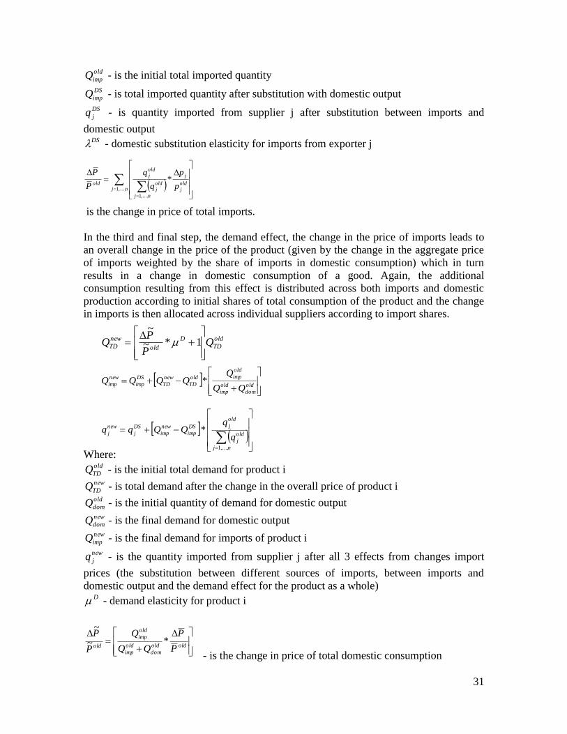
31
old
impQ - is the initial total imported quantity
DS
impQ - is total imported quantity after substitution with domestic output
DS
jq - is quantity imported from supplier j after substitution between imports and
domestic output DS - domestic substitution elasticity for imports from exporter j
is the change in price of total imports.
In the third and final step, the demand effect, the change in the price of imports leads to
an overall change in the price of the product (given by the change in the aggregate price
of imports weighted by the share of imports in domestic consumption) which in turn
results in a change in domestic consumption of a good. Again, the additional
consumption resulting from this effect is distributed across both imports and domestic
production according to initial shares of total consumption of the product and the change
in imports is then allocated across individual suppliers according to import shares.
Where: old
TDQ - is the initial total demand for product i new
TDQ - is total demand after the change in the overall price of product i old
domQ - is the initial quantity of demand for domestic output new
domQ - is the final demand for domestic output
new
impQ - is the final demand for imports of product i
new
jq - is the quantity imported from supplier j after all 3 effects from changes import
prices (the substitution between different sources of imports, between imports and
domestic output and the demand effect for the product as a whole) D - demand elasticity for product i
- is the change in price of total domestic consumption
oldold
dom
old
imp
old
imp
old P
P
Q
P
P*~
~
nj
old
j
old
jDS
imp
new
imp
DS
j
new
jq
qQQqq
,...,1
*
old
TD
D
old
new
TD QP
PQ
1*~
~
old
dom
old
imp
old
impold
TD
new
TD
DS
imp
new
impQQ
QQQQQ *
njold
j
j
nj
old
j
old
j
old p
p
q
q
P
P
,...,1
,...,1
*