assessing real estate returns by strategy: core v. value...
TRANSCRIPT

Joseph L. Pagliari, Jr. Clinical Professor of Real Estate
October 25, 2013 Chicago Booth Real Estate Conference
Chicago, Illinois
* Superior research support provided by Camilo Varela
Assessing Real Estate Returns by Strategy: Core v. Value-Added v. Opportunistic*

1 Core v. Non-Core Real Estate Returns
• What Do the Data Look Like?
• Promotes Create Asymmetries
• The Law of One Price
• Putting the Tools to Work: The Results
• Holding-Period Sensitivities
• Appendices – Other Sensitivities
– Dispersion in Fund Returns
Based on the PREA-Sponsored research paper: “An Overview of Fee Structures in Real Estate Funds and Their Implications for Investors” *
* Draft version of the PREA paper will be available on the Conference website.

0%
2%
4%
6%
8%
10%
12%
14%
16%
18%
0% 5% 10% 15% 20% 25%
Ave
rage
Ann
ual R
etur
ns
Volatility
Core Value-Added
Opportunistic
Source: NCREIF/Townsend and Author's Calculations
NPI
Gross Returns
Net Returns
Exhibit 62: Reported Performance by Fund Type for the 17-Year Period Ended December 31, 2012
2 Gross & Net Returns by Strategy
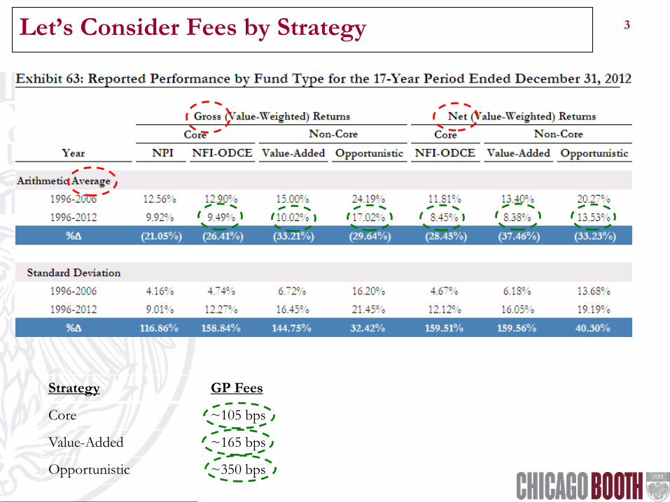
3 Let’s Consider Fees by Strategy
Strategy GP Fees
Core ~105 bps
Value-Added ~165 bps
Opportunistic ~350 bps

4 Volatility of Opp Fund Returns Looks Understated
Pre-Financial Crisis
Entire Time Period

5 Problems with the Data for Non-Core Returns
• Voluntary, Self-Reported Results
• Inconsistent Methodologies for Reporting
• Mark-to-Market Staleness
• Incomplete Capture of Fund Universe
• Incomplete Characterization of Funds: • domestic v. foreign, • debt v. equity, etc.
• Survivorship Bias ← only element we can attempt to correct
– Survivorship Bias = During & after the financial crisis, some funds stop reporting (without apparent termination)
– Survivorship Bias Adjustment (θ ) = Percentage of assets lost by non-reporting firms

6 Opp Returns with Survivorship-Bias Adjustment
0%
2%
4%
6%
8%
10%
12%
14%
16%
18%
15% 17% 19% 21% 23% 25% 27%
Ave
rage
Ann
ual R
etur
ns
Volatility
Source: NCREIF/Townsend and Author's Calculations
Exhibit 64: Reported Performance of the Opportunistic Funds for the 17-Year Period Ended December 31, 2012
with Survivorship Bias Adjustment (θ )
Source: NCREIF/Townsend and Author's Calculations
Gross Returns
Net Returns
θ = 0
θ = 0.5
θ = 1
θ = 0
θ = 0.5
θ = 1

7 Survivorship-Bias Adjusted Opp Returns
Ultimately, survivorship-bias adjustment does little to cure the suspected problem

8 Survivorship-Bias Adjusted Opp Returns in Context
0%
2%
4%
6%
8%
10%
12%
14%
16%
18%
0% 5% 10% 15% 20% 25%
Ave
rage
Ann
ual R
etur
ns
Volatility
CoreValue-Added
Opportunisitc
Source: NCREIF/Townsend and Author's Calculations
NPI
Gross Returns
Net Returns
Exhibit 66: Reported and Adjusted Performance by Fund Type for the 17-Year Period Ended December 31, 2012
θ= 0.5
θ= 0.5
9 Core v. Non-Core Real Estate Returns
• What Do the Data Look Like?
• Promotes Create Asymmetries
• The Law of One Price
• Putting the Tools to Work: The Results
• Holding-Period Sensitivities
• Appendices – Other Sensitivities
– Dispersion in Fund Returns
Based on the PREA-Sponsored research paper: “An Overview of Fee Structures in Real Estate Funds and Their Implications for Investors” *
* Draft version of the PREA paper will be available on the Conference website.

10 Numerical Example: Pref & Promote Structure
Fund-Level Return Distribution: Gross Return 13.0% Base Fees 1.0% Net Return 12.0% Volatility 15.0%
Fund Structure: Investor’s Preference 12.0% Residual Split:
– Investor 80% – General Partner 20%
Notes: – Investor’s preference typically set at or below fund’s likely return. – The general partner’s “promoted” interest creates an option-like
return for operator. – The value of the option reduces the investor’s upside.
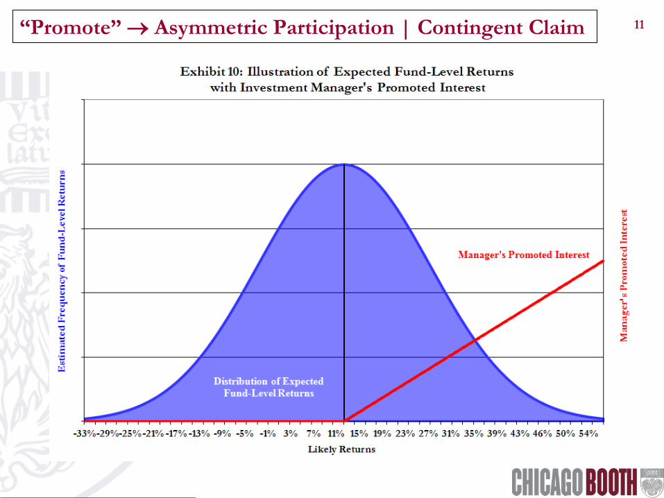
11 “Promote” → Asymmetric Participation | Contingent Claim
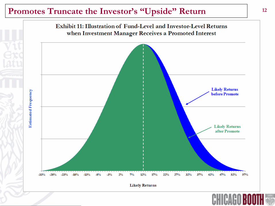
12 Promotes Truncate the Investor’s “Upside” Return

13 Numerical Example (continued)
Fund’s Gross and Net Returns: – Likely Returns:
Gross Return 13.0% Ongoing/Base Fees 1.0% Operating Partner’s Participation 1.2% Investor’s Net Return 10.8%
– Volatility (Standard Deviation): Fund-Level Volatility before General Partner 15.0% General Partner’s Participation 1.5% Investor’s Net Return 13.5%
Notes:
– The general partner’s “promoted” interest reduces the investor’s net return by 120 bps: Even though the value of the promote equals zero at the most likely return, This is attributable to general partner’s asymmetric participation in returns.
– The reduction in the investor’s standard deviation is a statistical illusion: The investor still receives 100% of the economic downside.

14 Point #1: Average Expectation ≠ Expectation of the Average
A simple way to the think of the average promote: Note: The appropriate way to calculate the expected promote: where: π = the “promote”, κ = general partner’s participation in the excess profits, ψ = investor’s preference, and f(x) = the distribution of fund-level returns, x.
Because of the general partner’s asymmetric participation: – The average expectation does not equal the expectation of the average :
( ) ( ) ( )E x f x dxψ
π κ ψ∞
= −∫
( ) ( ) ( ) ( )E x f x dx xψ
π κ ψ κ ψ∞
= − ≠ −∫
Exhibit 14: Simple, Two-Outcome Illustration of Asymmetric Payoffs
Gross NetOutcomes Probability Returns Promote Returns
Outcome1 50% 24.0% 2.4% 21.6%
Outcome2 50% 0.0% 0.0% 0.0%
Average 12.0% 1.2% 10.8%
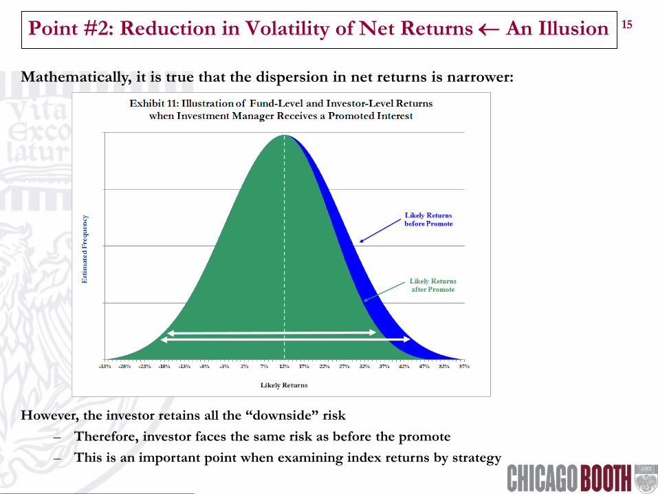
15 Point #2: Reduction in Volatility of Net Returns ← An Illusion
Mathematically, it is true that the dispersion in net returns is narrower: However, the investor retains all the “downside” risk
– Therefore, investor faces the same risk as before the promote – This is an important point when examining index returns by strategy

16 Core v. Non-Core Real Estate Returns
• What Do the Data Look Like?
• Promotes Create Asymmetries
• The Law of One Price
• Putting the Tools to Work: The Results
• Holding-Period Sensitivities
• Appendices – Other Sensitivities
– Dispersion in Fund Returns
Based on the PREA-Sponsored research paper: “An Overview of Fee Structures in Real Estate Funds and Their Implications for Investors” *
* Draft version of the PREA paper will be available on the Conference website.

17 Use the “Law of One Price” to Create Risk/Return Continuum
E
xpec
ted
Ret
urn
(ke)
Expected Volatility (σe)
Exhibit 68: Illustration of "Law of One Price"Lever Core Assets to Create Risk/Return Continuum
ke : Levered Core Fund Returns 0% Leverage
25% Leverage
50% Leverage
75% Leverage
ka : Unlevered Core Fund Returns

18 Law of One Price → Risk-Adjusted Returns: “Alpha” (α )
E
xpec
ted
Ret
urn
(ke)
Expected Volatility (σe)
Exhibit 69: Application of "Law of One Price"Levered Core Assets v. Non-Core Funds
ke : Levered Core Fund Returns 0% Leverage
25% Leverage
50% Leverage
75% Leverage
Out-PerformingNon-Core Fund
Under-Performing Non-Core Fund
ka : Unlevered Core Fund Returns
Positive Alpha
Negative Alpha

19 Interest Rates =f(LTV|Asset Quality, Sponsorship, etc.)
0% 15% 30% 45% 60% 75%
Inte
rest
Rat
e pe
r A
nnum
(k d
)
Loan-to-Value Ratio
Exhibit 67: Illustration of the Cost of Indebtedness as a Function of Leverage
Risk-free Rate
Mortgage Interest Rate
Default Risk (δ) Premium
Structural Differences (γ) in Payment Schedules, Servicing Fees, Etc .
Relationship is for a given moment in
time

20 Risk-Free Rates & Spreads Vary Over Time
0%
2%
4%
6%
8%
10%
12%
1996 1997 1998 1999 2000 2001 2002 2003 2004 2005 2006 2007 2008 2009 2010 2011 2012
Est
imat
ed A
nnua
l Int
eres
t Exp
ense
(kd
)
Exhibit 71: Estimates of the Annual Interest Rateat Various Leverage Ratios for the Years 1996 through 2012
Risk-free Rate
Interest Expense at 75% LTV
Interest Expense at 50% LTV
Interest Expense at 25% LTV
Structural Differences (γ)
Changes Over Time:
1. Risk-free
Rate, and
2. Spreads:
a) low before the financial crisis,
b) spiked up during and after the financial crisis, and
c) have started to recede thereafter

21 Core v. Non-Core Real Estate Returns
• What Do the Data Look Like?
• Promotes Create Asymmetries
• The Law of One Price
• Putting the Tools to Work: The Results
• Holding-Period Sensitivities
• Appendices – Other Sensitivities
– Dispersion in Fund Returns
Based on the PREA-Sponsored research paper: “An Overview of Fee Structures in Real Estate Funds and Their Implications for Investors” *
* Draft version of the PREA paper will be available on the Conference website.
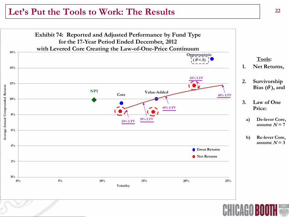
22 Let’s Put the Tools to Work: The Results
0%
2%
4%
6%
8%
10%
12%
14%
16%
0% 5% 10% 15% 20% 25%
Ave
rage
Ann
ual C
ompo
unde
d R
etur
ns
Volatility
Exhibit 74: Reported and Adjusted Performance by Fund Type for the 17-Year Period Ended December, 2012
with Levered Core Creating the Law-of-One-Price Continuum
NPI Value-AddedCore
Opportunistic ( θ =.5)
Gross Returns
Net Returns
24% LTV
60% LTV
45% LTV
35% LTV
55% LTV
Tools: 1. Net Returns,
2. Survivorship
Bias (θ ), and
3. Law of One Price:
a) De-lever Core, assume N = 7
b) Re-lever Core, assume N = 3

23 Let’s Put the Tools to Work: The Results (continued)
0%
2%
4%
6%
8%
10%
12%
14%
16%
0% 5% 10% 15% 20% 25%
Ave
rage
Ann
ual C
ompo
unde
d R
etur
ns
Volatility
Exhibit 75: Reported & Volatility-Adjusted Performance by Fund Type for the 17-Year Period Ended December, 2012
with Levered Core Creating the Law-of-One-Price Continuum
NPI Value-AddedCore
Opportunistic(θ = .5)
Gross Returns
Net Returns - UnadjustedNet Returns - Volatility-Adjusted
Tools: 1. Net Returns,
2. Survivorship Bias (θ ), and
3. Law of One Price
4. Volatility Adjustment (correct for statistical illusion)
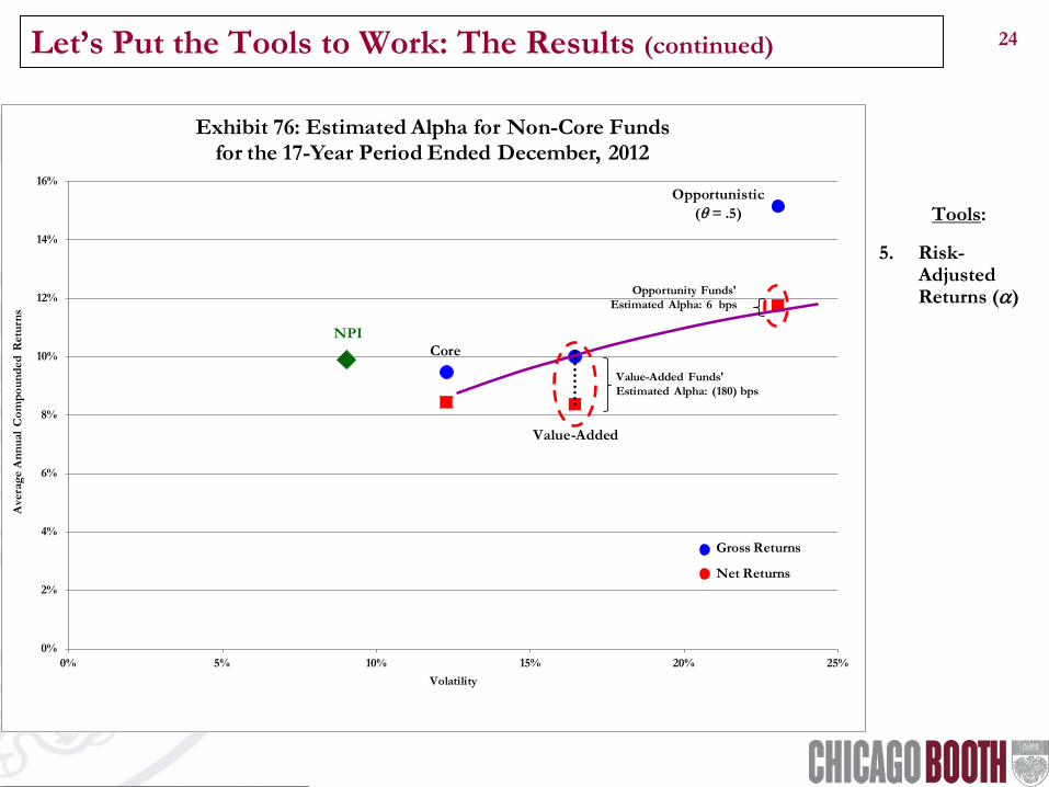
24 Let’s Put the Tools to Work: The Results (continued)
0%
2%
4%
6%
8%
10%
12%
14%
16%
0% 5% 10% 15% 20% 25%
Ave
rage
Ann
ual C
ompo
unde
d R
etur
ns
Volatility
Exhibit 76: Estimated Alpha for Non-Core Funds for the 17-Year Period Ended December, 2012
NPI
Value-Added
Core
Opportunistic(θ = .5)
Gross Returns
Net Returns
Value-Added Funds' Estimated Alpha: (180) bps
Opportunity Funds' Estimated Alpha: 6 bps
Tools: 1. Net Returns,
2. Survivorship Bias (θ ), and
3. Law of One Price 4. Volatility Adjustment
5. Risk-Adjusted Returns (α)

25 Let’s Put the Tools to Work: The Results (continued)
0%
2%
4%
6%
8%
10%
12%
14%
16%
0% 5% 10% 15% 20% 25%
Ave
rage
Ann
ual C
ompo
unde
d R
etur
ns
Volatility
Exhibit 76: Estimated Alpha for Non-Core Funds for the 17-Year Period Ended December, 2012
NPI
Value-Added
Core
Opportunistic(θ = .5)
Gross Returns
Net Returns
Value-Added Funds' Estimated Alpha: (180) bps
Opportunity Funds' Estimated Alpha: 6 bps
Results:
For Opportunistic Funds, an
“efficient market” type answer :
investors receive a “fair” return,
while managers receive the “surplus”
For Value-Added Funds, no such
answer : dramatic under-
performance

26 Core v. Non-Core Real Estate Returns
• What Do the Data Look Like?
• Promotes Create Asymmetries
• The Law of One Price
• Putting the Tools to Work: The Results
• Holding-Period Sensitivities
• Appendices – Other Sensitivities
– Dispersion in Fund Returns
Based on the PREA-Sponsored research paper: “An Overview of Fee Structures in Real Estate Funds and Their Implications for Investors”*
* Draft version of the PREA paper will be available on the Conference website.

27 Time-Varying Returns | The Market for Core Assets
Any fair comparison examines a
complete market cycle
In a market
downturn, there is a “flight to
quality” → non-core assets are hit
harder
Let’s consider returns by
“vintage” by strategy

28 “Mountain” Chart for Value-Added Index’s Alpha
• Repeat the earlier (α ) exercise for differing vintages
• Choose any beginning and ending date, with minimum 6-year hold
• Value-add funds underperform before, during & after the financial crisis • The pre-financial-crisis underperformance is particularly damning!
Our earlier result

29 “Mountain” Chart for Opportunistic Index’s Alpha
• Repeat the earlier (α ) exercise for differing vintages
• The index of Opportunistic funds underperforms before the financial crisis
• Yet, they overperform during & after the financial crisis! • How can this be? It cannot [=f(“flight to quality”)] • Provides another perspective on data problems & survivorship bias
Our earlier result

30 Core v. Non-Core Real Estate Returns
• What Do the Data Look Like?
• Promotes Create Asymmetries
• The Law of One Price
• Putting the Tools to Work: The Results
• Holding-Period Sensitivities
• Appendices – Other Sensitivities: θ = .5, NCore = 5 & NOpp = 3
– Dispersion in Fund Returns
Based on the PREA-Sponsored research paper: “An Overview of Fee Structures in Real Estate Funds and Their Implications for Investors” *
* Draft version of the PREA paper will be available on the Conference website.

31 The Sensitivity of Survivorship-Bias Adjustment (θ )
Results:
θ = 0
θ = .5 (base case)
θ = 1
As you’d suspect: α↓ as θ↑
Range ≈ 410 bps
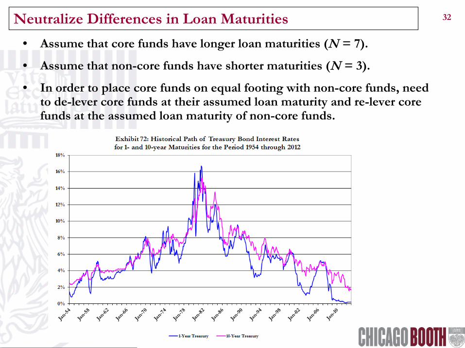
32 Neutralize Differences in Loan Maturities
• Assume that core funds have longer loan maturities (N = 7).
• Assume that non-core funds have shorter maturities (N = 3).
• In order to place core funds on equal footing with non-core funds, need to de-lever core funds at their assumed loan maturity and re-lever core funds at the assumed loan maturity of non-core funds.

33 The Sensitivity of Assumed Core Debt Maturity (NCore )
Results:
ΝCore = 5
ΝCore = 7 (base case)
ΝCore = 10
As you’d suspect: α↓ as Νcore ↑
Range ≈ 40 bps
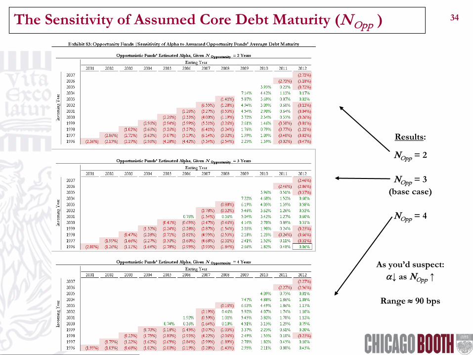
34 The Sensitivity of Assumed Core Debt Maturity (NOpp )
Results:
ΝOpp = 2
ΝOpp = 3 (base case)
ΝOpp = 4
As you’d suspect: α↓ as ΝOpp ↑
Range ≈ 90 bps
35 Core v. Non-Core Real Estate Returns
• What Do the Data Look Like?
• Promotes Create Asymmetries
• The Law of One Price
• Putting the Tools to Work: The Results
• Holding-Period Sensitivities
• Appendices – Other Sensitivities
– Dispersion in Fund Returns
Based on the PREA-Sponsored research paper: “An Overview of Fee Structures in Real Estate Funds and Their Implications for Investors” *
* Draft version of the PREA paper will be available on the Conference website.

36 Note: An Index v. Individual Funds
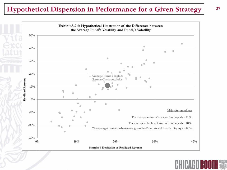
37 Hypothetical Dispersion in Performance for a Given Strategy
-30%
-20%
-10%
0%
10%
20%
30%
40%
50%
0% 10% 20% 30% 40%
Rea
lized
Ret
urns
Standard Deviation of Realized Returns
Exhibit A.2.6: Hypothetical Illustration of the Difference between the Average Fund's Volatility and Fundi's Volatility
Average Fund's Risk & Return Characteristics
Major Assumptions:
The average return of any one fund equals ~11%.
The average volatility of any one fund equals ~18%.
The average correlation between a given fund's return and its volatility equals 80%.
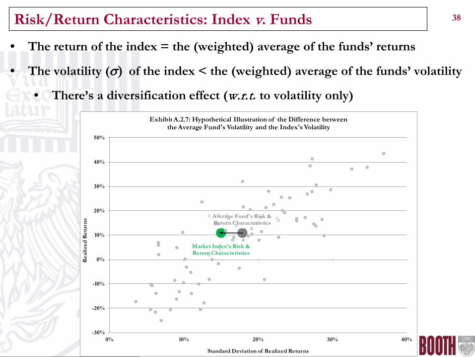
38 Risk/Return Characteristics: Index v. Funds
-30%
-20%
-10%
0%
10%
20%
30%
40%
50%
0% 10% 20% 30% 40%
Rea
lized
Ret
urns
Standard Deviation of Realized Returns
Exhibit A.2.7: Hypothetical Illustration of the Difference between the Average Fund's Volatility and the Index's Volatility
Average Fund's Risk & Return Characteristics
Market Index's Risk & Return Characteristics
• The return of the index = the (weighted) average of the funds’ returns
• The volatility (σ) of the index < the (weighted) average of the funds’ volatility
• There’s a diversification effect (w.r.t. to volatility only)

39 Risk/Return Characteristics: Index v. Funds (continued)
• Consider the dispersion around the (weighted) average of the funds’ returns • not the index’s return!
• Each ellipse contains a certain proportion of fund returns:
-30%
-20%
-10%
0%
10%
20%
30%
40%
50%
0% 10% 20% 30% 40%
Rea
lized
Ret
urns
Standard Deviation of Realized Returns
Exhibit A.2.8: Hypothetical Illustration of the Difference between the Average Fund's Volatility and the Index's Volatility
Average Fund's Risk & Return Characteristics
Market Index's Risk & Return Characteristics

40 Risk/Return Characteristics: Index v. Funds (continued)
• This diversification effect is greatest with opportunistic funds • → biggest difference between index’s σ and the average fund’s σ • → need more opp funds to be well diversified (within that strategy)
• Under-diversified opp-fund investors experience greatest decline in α
0%
5%
10%
15%
20%
25%
0% 5% 10% 15% 20% 25% 30% 35% 40%
Exp
ecte
d R
etur
n (k
e)
Expected Volatility (σe)
Exhibit A.2.9: Illustration of the Law of One PriceLever Core Assets to Create Risk/Return Continuum
25% Leverage = Core Index
40% Leverage = Value-Add Index
60% Leverage = Opportunity Index
ka : Unlevered Core Fund Returns
ke : Levered Core Fund Returns
To be effectively diversified (i.e., within 50 bps of an index’s volatility) and given my underlying assumptions, an investor would need:
• ≥ 2 core funds,
• ≥ 7 value-add funds, &
• ≥ 15 opportunity funds.