Vilnius University

Faculty of Physics

Department of Solid State Electronics

Laboratory of Atomic and Nuclear Physics

Experiment No. 8

ARTIFICIAL RADIOACTIVITY

by Andrius Poškus

(e-mail: andrius.poskus@ff.vu.lt)

2010-06-27

Contents

The aim of the experiment 2

1. Tasks 2

2. Control questions 2

3. The law of radioactive decay. Activation by neutron capture 3

4. Experimental setup 6

5. The measurement procedure 7

6. Analysis of experimental results 13

2

The aim of the experiment Test the exponential law of radioactive decay, measure half-lives of radioactive nuclides from their decay curves, investigate the phenomenon of activity saturation.

1. Tasks

1. Measure the decay curve of a silver sample, initially consisting of 51,35 % (silver-107) and 48,65 % (silver-109) after its bombardment by neutrons (activation). Repeat those measurem es, each one corresponding to a different activation time.

2. Plot the decay curves of the mixture of radioactive nuclides 108Ag (silver-108) and 110Ag (silver-110) and use those curves to calculate the half-life of 108Ag.

3. Plot the activation curve of 108Ag.

4. Using the calculated half-life of 108Ag, isolate and plot the contribution of 110Ag to the overall decay curve and calculate the half-life of 110Ag.

5. Discuss the results.

2. Control questions

1. What is the nucleus and what are its constituents? Explain the concepts of isotopes and isobars.

2. What is nuclear binding energy? How is it related to the mass of the nucleus?

3. What is radioactivity? What are the types of radioactive decay? How is the kinetic energy of decay products related to masses of the parent nucleus and decay products (use the principle of mass-energy equivalence)?

4. What is the time dependence of the number of radioactive nuclei? What is the decay constant and the half-life?

5. What is the activity of a radioactive substance? How does the activity depend on time?

6. Explain the concept of nuclear reaction. What is the difference between nuclear reaction and radioactive decay?

7. Explain the concept of radiative neutron capture.

8. Explain the concept of a nuclear reaction cross-section. Why neutrons must be slowed down (“moderated”) when they are used to created new nuclides by the capture reaction?

9. Why the best neutron moderators are the materials containing large quantities of hydrogen atoms?

10. The concepts of activation and activation curve. Whey the activity of the sample that is being bombarded with neutrons stops increasing after a certain time?

11. Why the most likely type of radioactive decay of a substance created by neutron capture is the β– (“beta minus”) decay?

12. Does the number of silver atoms change after the activation of the silver sample and its complete deactivation?

Recommended reading:

1. Krane K. S. Introductory Nuclear Physics. New York: John Wiley & Sons, 1988. p. 160 − 165, 169 – 170, 173 – 175, 217 – 220, 230 – 231, 378 − 380, 392 − 394, 416 − 421, 447 − 451, 456 – 459.

2. Lilley J. Nuclear Physics: Principles and Applications. New York: John Wiley & Sons, 2001. p. 3 – 42, 93 − 104, 108 – 110, 113 – 116, 142 − 148, 212 – 213.

3. Knoll G. F. Radiation Detection and Measurement. 3rd Edition. New York: John Wiley & Sons, 2000. p. 21 – 23, 55 – 57.

10747 Ag

10947 Ag

ents 4 tim

3

3. The law of radioactive decay. Activation by neutron capture It is known that the number of atoms of radioactive nuclear species (nuclide) decreases exponentially with time:

0( ) e tN t N λ−= , (3.1) where N(t) is the number of atoms (nuclei) at time t, N0 is the initial number of nuclei (at time t = 0), and λ is the decay constant. The decay constant determines the rate at which the number of radioactive nuclei decreases: the larger the decay constant, the faster the radioactive decay. Another way to specify the rate of decrease of the number of radioactive nuclei is by specifying the half-life, which is related to the decay constant as follows:

1/ 2ln2Tλ

= . (3.2)

The half-life is the time needed for the number of radioactive nuclei to decrease by half. Equation (3.1) is the formulation of the so-called “law of radioactive decay”. An equivalent way to formulate it is to take time derivatives of both sides of the equation:

ddN Nt

λ= − . (3.3)

This is the first-order differential equation whose solution corresponding to initial condition N(0) = N0 is (3.1). The left side of this equation is opposite to the rate of decay (the number of atoms decaying per unit time). The rate of decay is the so-called activity of the sample. Since N decreases with time, from Eq. (3.3) it follows that activity also decreases exponentially with time:

0d( ) ( ) ed

tNt N t Nt

λΦ λ λ −≡ − = = . (3.4)

The logarithm of this function is a straight line (see Fig. 1). Its intercept gives the logarithm of the initial activity ln(λ N0), and its slope is the opposite of the decay constant (−λ). Thus, analysis of the decay curve is a simple method of determining the decay constant λ and the half-life T1/2. If a radioactive source is composed of several radioactive nuclides, then the total activity of the source is equal to the sum of activities of constituent nuclides. If those nuclides are independent (i. e. if neither of them is a product of decay of another nuclide present in the same sample), then the overall decay curve is a sum of several exponential terms. For example, in the case of two independent radioactive nuclides

2t1 2 11 2 01 02 1 01 2 02e e e et t tN Nλ λ λΦ Φ Φ Φ Φ λ λ λ− − −= + = + = + − , (3.5)

where Φ1 and Φ2 activities of the two nuclides, Φ01 and Φ02 are the corresponding initial activities, λ1 and λ2 are the decay constants, N01 and N02 are the initial quantities of both nuclides. In this case the time dependence of the logarithm of activity consists of two linear regions and a transition region between them (see Fig. 2). In this experiment, the investigated substance is silver. Natural silver consists of two stable isotopes – and (51,35 % and 48,65 % ). When those isotopes are bombarded by neutrons, the following nuclear reactions take place:

10747 Ag 109

47 Ag 10747 Ag 109

47 Ag

107 1 10847 0 47Ag n Ag γ+ → + , (3.6a)

109 1 11047 0 47Ag n Ag γ+ → + . (3.6b)

Fig. 1. Time dependence of the natural logarithm of activity

Fig. 2. Time dependence of the natural logarithm of activity of a mixture of two independent radioactive nuclides

ln(λN0e−λt) = ln(λN0) − λt

0

ln(λN0)

t

lnΦ

ln(λ2N02)

lnΦ2(t)lnΦ1(t)

lnΦ = ln(Φ1+Φ2)

0

ln(λ1N01+λ2N02)

t

lnΦ

4

The reaction products and are β− radioactive. I. e., they subsequently decay as follows: 10847 Ag 110

47 Ag108 10847 48 e

142sAg Cd e ν−+ +→ , (3.7a)

110 11047 48 e

24,6sAg Cd e ν−+ +→ (3.7b)

(half-lives are indicated under the arrows). The process of creating radioactive nuclides by neutron bombardment is called activation. After activation of a silver sample, its total activity decays with time as a sum of two exponentially decaying terms (3.5). However, in this experiment, the quantity that is measured directly is not the activity, but the number of beta particles detected by the Geiger-Müller counter over a fixed interval of time, Δn(t). Fortunately, the number of detected particles is proportional to activity, therefore the overall shape of the function Δn(t) is the same as that of the function Φ(t), i. e. it is a sum of two exponents:

1 21 2( ) e et tn t C Cλ λ− −Δ = + , (3.8)

where Δn(t) is the number of particles detected during the interval of time starting at t − Δt and ending at t (here Δt denotes the measurement interval length). In Eq. (3.8), the first term corresponds to 108Ag, and the second term corresponds to 110Ag. Since decay of 108Ag is slower than decay of 110Ag, let us call the first term the “slow component” and the second term the “fast component”. The coefficients C1 and C2 depend on detector parameters, measurement geometry (i. e. the shape of the sample and its position relative to the detector), activation time ta and the duration of a single measurement Δt. In this experiment, only the latter two quantities are variable: decay curves are measured after four activation, each with a different activation time ta, and there are two values of Δt used (during the first two minutes of each decay curve, the measurement interval is 10 s, and later on it is 60 s). Since ta is variable, it becomes possible to investigate not only the shape of individual decay curves, but also the dependence of that shape on ta. Clearly, only the preexponential factors C1 and C2 depend on ta (the decay constants λ1 and λ2 can not depend on ta, because those constants are internal parameters of the nuclides, and activation only changes the number of nuclei, not their internal properties). The pre-exponential factors are proportional to activities of corresponding nuclides at the end of activation. Let us discuss dependence of activity on activation time ta. From Eq. (3.4) we know that activity is proportional to the number of radioactive nuclei. The dependence of the quantity of a particular nuclide on ta during the activation can be determined from the differential equation

pddN N j Nt

σ λ= − , (3.9)

where N is the number of atoms of the daughter nuclide, Np is the number of atoms of the parent nuclide, σ is the neutron capture cross-section and j is the density of neutron flux (i. e. the number of neutrons per unit area per unit time). If we compare Eq. (3.9) with the law of radioactive decay (3.3), we can see that there is an additional term ( pN jσ ) on the right-hand side of the equation. This term reflects the fact that during the act ; they are also created due to neutron capture. Thus, there are two competing processes: an increase of the number of daughter nuclei due to neutron capture (this increase is reflected by

ivation, the nuclei not only decay

the positive term pN jσ ease is reflectders of m

constant. Thus,

i N). This value of

in Eq. (3.9)), and the decrease of that number due to decay of the daughter nuclei (this decr ed by the negative term −λN). Since the number of nuclei that capture a neutr ny or agnitudes smaller than the number of parent nuclei Np, the latter number can be assu e the first term on the right-hand side of Eq. (3.9) is practically constant, whereas the absolute value of the second term increases with time (due to the increase of the number of e means that the increase of N during activation slows down continuously and ev the N stabilizes. This happens when the rate of nuclide production (

on is mamed to b

daughter nuclentually

pN jσ ) becomes eq λN). This stable value of N is called the „saturation value“. The mathematical expression of dependence of N on ta is obtained by solving the differential equation (3.9) with initial condition N(0) = 0. This solution is

ual to the rate of its decay (

aa sat( ) (1 e )tN t N λ−= − , (3.10)

where Nsat is the mentioned saturation value of the number of radioactive nuclei. The corresponding dependence of activity on activation time has the same shape:

aa a sat( ) ( ) (1 e )tt N t N λΦ λ λ −= = − . (3.11)

5

This function is shown in Fig. 3. Obviously, the number of daughter nuclei (and activity) saturates after a time which is roughly equal to 4 – 5 half-lives. As mentioned above, the pre-exponential factors in Eq. (3.8) are proportional to corresponding activities at the end of activation. Therefore, their dependence on activation time ta is also of the shape defined by Eq. (3.11) and shown in Fig. 3. In particular, dependence of the factor C1 (which corresponds to the longer-lived nuclide 108Ag) on ta is the following:

Φ

a11 a 1,sat( ) (1 e )tC t C λ−= − , (3.12)

where C1,sat is the saturation value of C1. Now, let us discuss the dependence of C1 on duration of a single count Δt. Since the number of particles detected per unit time is proportional to activity of the sample, the number of particles detected during the period from t − Δt to t is proportional to the integral of activity during the same period. From this it follows that C1 is proportional to exp(λ1Δt) − 1. Thus, if C1 denotes the value of the pre-exponential factor corresponding to Δt = 60 s, and 1C′ denotes its value corresponding to Δt = 10 s, then those two values are related as follows:

1

1

10s

1 160se 1e 1

C Cλ

λ

⋅

⋅

−′ =−

. (3.13)

Using the decay constant of 108Ag ( 11 ln 2 /(142,2s) 0,00487 sλ −= = ), the following expression of 1C′ is

obtained from (3.13): Some of the detected particles may be emitted by other radioactive sources (e. g. cosmic radiation or natural radioactivity of the environment). Those particles show up as a constant term in the measured count. This term is referred to as the “background”. Eq. (3.8) corresponds to the ideal case when the background is zero. In general, one must take into account the background term Δnb:

b

1 10,147C C′ = .

1 21 2( ) e et tn t C C nλ λ− −Δ = + + Δ . (3.14)

The background term Δnb is measured when the investigated sample is sufficiently far away from the detector.

Fig. 3. Activation curve as (1 e )tλΦ Φ −= − . ta is activation time, Φ is activity of the sample, Φs is

the saturation activity, λ is the decay constant

5T1/24T1/23T1/22T1/2T1/2

Φs0,938Φs0,875Φs

0,75Φs

0,5Φs

0ta

6

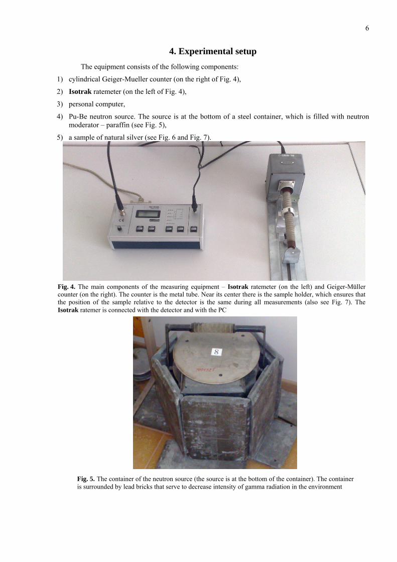
4. Experimental setup The equipment consists of the following components:

1) cylindrical Geiger-Mueller counter (on the right of Fig. 4),

2) Isotrak ratemeter (on the left of Fig. 4),

3) personal computer,

4) Pu-Be neutron source. The source is at the bottom of a steel container, which is filled with neutron moderator – paraffin (see Fig. 5),

5) a sample of natural silver (see Fig. 6 and Fig. 7).

Fig. 4. The main components of the measuring equipment – Isotrak ratemeter (on the left) and Geiger-Müller counter (on the right). The counter is the metal tube. Near its center there is the sample holder, which ensures that the position of the sample relative to the detector is the same during all measurements (also see Fig. 7). The Isotrak ratemer is connected with the detector and with the PC

Fig. 5. The container of the neutron source (the source is at the bottom of the container). The container is surrounded by lead bricks that serve to decrease intensity of gamma radiation in the environment

7

5. The measurement procedure During this experiment, four decay curves (3.14) of the mixture of radioactive silver isotopes 108Ag and 110Ag are measured. Each of them corresponds to a different activation time ta. Approximate values of the activation time are the following: 10 min, 5 min, 2 min and 1 min. After each activation, the decay curve is measured for 10 min, then the sample is placed away from the detector and the background is measured for additional 10 min (during this time, the silver sample completely deactivates and becomes ready for the next activation-deactivation cycle). Since each decay curve consists of two components – the slow one (it corresponds to decay of 108Ag) and the fast one (it corresponds to decay of 110Ag), two values of the counting time Δt are used: during the first 2 minutes it is Δt = 10 s, and during the last 8 minutes it is Δt = 60 s. I. e., in the initial part of the decay curve each point gives the number of particles detected during last 10 s, and in the final part of the decay curve each point gives the number of particles detected during last 60 s. The computer program that receives data from the Isotrak ratemeter passes that data to the program “Origin 6” in real time. The program “Origin 6” displays the data in the form of worksheets and graphs. Fig. 8 shows an example of the Origin graph. The vertical bars centered on each point are the so-called “error bars”. The length of each error bar is twice the standard deviation of each measurement result (one standard deviation upwards from the point and one standard deviation downwards from the point). Those standard deviations are calculated under the assumption of Poisson distribution. I. e.

Fig. 6. The silver sample and its handle

Fig. 7. The detector and the silver sample during the measurement of the decay curve

8

standard deviation of each measurement result is equal to the square root of that result (the standard deviations will be subsequently used for calculating weight factors during nonlinear fitting). The following conventions regarding the times are used in the graphs with decay curves:

1) The time t, which is plotted on the X axis, is counted from the moment of time corresponding to the end of activation. Thus, the time t = 0 corresponds to extraction of the sample from the neutron source (and not to placement of the sample upon the detector!).

2) The time corresponding to each point is time of the end of the corresponding count. For example, if a point is at t = 30 s, this means that this point is the number of particles detected during the time interval 20 s < t < 30 s.

As extraction of the sample from the neutron source and its placement upon the detector lasts for several seconds, the first point (at t = 10 s) is inaccurate. This is because the position of the sample relative to the detector during the time interval 0 < t < 10 s is different from that position during the subsequent measurements. Hence, the first point is not used for fitting (if necessary, more points can be removed prior to fitting, too).

A detailed step-by-step procedure of the measurements is given below.

1. Switch on the PC and the Isotrak ratemer. Set the detector voltage to (450 ± 20) V. In order to do that, it is necessary to press the button “Select” on the Isotrak ratemeter several times until the LED “G-M Voltage” starts blinking, and press the button “Enter”. Then the display of the ratemeter shows the detector voltage (in volts). The voltage can be adjusted by turning a knob that is in the lower left corner of the Isotrak ratemeter.

2. Start the program “Activ.exe”, which receives data from the Isotrak ratemeter and passes it to the program “Origin 6.1”. The program “Activ.exe” is in the folder “C:\Artificial_Radioactivity”. It can also be started using a Start Menu shortcut. The initial window of the program “Activ.exe” is shown in Fig. 9a.

Fig. 8. An example of a decay curve

9

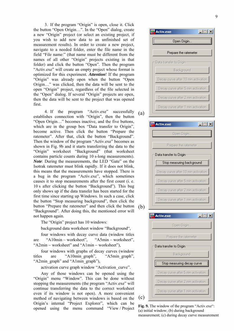
3. If the program “Origin” is open, close it. Click the button “Open Origin…”. In the “Open” dialog, create a new “Origin” project (or select an existing project, if you wish to add new data to an unfinished set of measurement results). In order to create a new project, navigate to a needed folder, enter the file name in the field “File name:” (that name must be different from the names of all other “Origin” projects existing in that folder) and click the button “Open”. Then the program “Activ.exe” will create an empty project whose format is optimized for this experiment. Attention! If the program “Origin” was already open when the button “Open Origin…” was clicked, then the data will be sent to the open “Origin” project, regardless of the file selected in the “Open” dialog. If several “Origin” projects are open, then the data will be sent to the project that was opened first.

4. If the program “Activ.exe” successfully establishes connection with “Origin”, then the button “Open Origin…” becomes inactive, and the five buttons, which are in the group box “Data transfer to Origin”, become active. Then click the button “Prepare the ratemeter”. After that, click the button “Background”. Then the window of the program “Activ.exe” becomes as shown in Fig. 9b and it starts transferring the data to the “Origin” worksheet “Background” (that worksheet contains particle counts during 10 s-long measurements). Note: During the measurements, the LED “Gate” on the Isotrak ratemeter must blink rapidly. If it does not blink, this means that the measurements have stopped. There is a bug in the program “Activ.exe”, which sometimes causes it to stop measurements after the first count (i. e. 10 s after clicking the button “Background”). This bug only shows up if the data transfer has been started for the first time since starting up Windows. In such a case, click the button “Stop measuring background”, then click the button “Prepare the ratemeter” and then click the button “Background”. After doing this, the mentioned error will not happen again.

The “Origin” project has 10 windows: background data worksheet window “Background“, four windows with decay curve data (window titles

are “A10min − worksheet”, “A5min − worksheet”, “A2min − worksheet” and “A1min − worksheet”),

four windows with graphs of decay curves (window titles are “A10min_graph”, “A5min_graph”, “A2min_graph” and “A1min_graph”),

activation curve graph window “Activation_curve”. Any of those windows can be opened using the

“Origin” menu “Window”. This can be done without stopping the measurements (the program “Activ.exe” will continue transferring the data to the correct worksheet even if its window is not open). A more convenient method of navigating between windows is based on the Origin’s internal “Project Explorer”, which can be opened using the menu command “View / Project Fig. 9. The window of the program “Activ.exe“:

(a) initial window; (b) during background measurement; (c) during decay curve measurement

(a)

(b)

(c)

10

Explorer”. In the latter case, it is recommended to use the Project Explorer view mode “List” (in order to change the view mode, right-click anywhere in the Project Explorer pane and then select “View / List” from the menu).

5. Take off the lid from the container of the neutron source (then the container looks as shown in Fig. 10a). After that, uncover the slit for insertion of the sample (i. e. pull the two narrow lead bricks to the sides as shown in Fig. 10b).

6. Insert the sample into the neutron source container (see Fig. 11). When the sample is fully

inserted (as shown in Fig. 11b), start measuring the activation time. It can be measured using any clock that shows seconds. The duration of the first activation is approximately 10 min (also see the note in Step 11). During that time, measure the background.

7. The next step is measuring the decay curve. Unlike the background measurement, the start of

the decay curve measurement must be synchronized with activation end. Therefore, it is recommended to stop measuring the background with enough time left until the end of activation, so that the preparation for decay curve measurements can be done in time. Since this preparation requires less than 10 s, background measurements can be stopped with 20 s or 30 s remaining. In order to stop background measurement, click the button “Stop measuring background”. After that, click the button “Prepare the ratemeter”. This ends the preparation for decay curve measurement.

Fig. 10. The container of the neutron source: (a) without the lid; (b) with the sample slit uncovered (a) (b)

(a) (b) Fig. 11. Insertion of the sample into the neutron source container: (a) start; (b) end (the screw that is fastened upon the sample handle must touch the top of the container)

11

8. When the required time has passed since the start of activation (e. g., 600 s), extract the sample from the neutron source and at the same time click one of the four buttons “Decay curve …” (for example, after the longest activation click “Decay curve after 10 min activation”). Then the “Activ.exe” window becomes as shown in Fig. 9c and the program begins automatic data transfer to the corresponding “Origin” worksheet. For example, after clicking “Decay curve after 10 min activation” the data will be recorded in the worksheet “A10min − worksheet” and simultaneously shown in the graph “A10min_graph”.

9. Place the sample upon the detector as shown in Fig. 7 and Fig. 12. Ideally, the total time of sample extraction from the neutron source and its placing upon the detector should be less than 10 s (then no additional data modifications will be needed in the future). If a longer time has passed, then take notice of the number of initial points that will have to be excluded from fitting. For example, if the mentioned time is 25 s, then three initial counts will have to be removed (their approximate intervals are 0 − 10 s, 10 s − 20 s and 20 s − 30 s, counting from the end of activation)

10. When 10 min passes since the start of the decay curve measurement, the program “Activ.exe”

stops the measurement automatically (then the button “Background” and all four buttons “Decay curve” become active again). Then place the silver sample away from the detector (a distance of 1 − 2 m is sufficient) and wait for 10 min until the sample completely de-activates. During that 10 min interval, measure background again. In order to continue background measurements, click the buttons “Prepare the ratemeter” and “Background”.

Fig. 12. Positioning of the silver sample on the detector while measuring the decay curve: (a) the end of the aluminum handle where sample is fastened must be pushed all the way into the holder; (b) the handle must be inside the cut of the detector stand

(a)

(b)

12

11. Repeat Steps 6 – 10 with a different activation time. In this way, four activation-deactivation cycles must be done, which correspond to activation times 10 min, 5 min, 2 min and 1 min. Decay curve must be measured for 10 min (regardless of the activation time), and then additional 10 minutes must pass in order for the sample to completely deactivate. However, after measuring the fourth decay curve, it is not necessary to wait until complete deactivation (and to measure the background). Note: The mentioned activation times are approximate. They have been chosen based on the requirement that one activation time is 2 − 5 times shorter than 108Ag half-life, another one is close to the half-life, the third one is 2 − 3 times longer than the half-life and the fourth one is 4 − 5 times longer than the half-life. Another set of activation times may be chosen (e. g., 12 min, 4 min, 1,5 min and 0,5 min). The true activation time (in seconds) must be specified in the text field that is at the top of the corresponding “Origin” graph (“Origin” reads the activation times from those fields). However, for correct functioning of the scripts that are associated with buttons visible on the right of the “Origin” project windows, the window titles must not be changed (for example, the titles of the windows corresponding to the longest activation time must be “A10min − worksheet” and “A10min_graph”, even if the corresponding true activation time is 12 min).

12. After ending the measurements, save the measurement data (“Origin” menu command „File / Save Project“ or „File / Save Project As...“), switch off the Isotrak ratemeter, cover the neutron source and print the worksheet data of all four decay curves. The printed numbers must not be processed (i. e., no background subtracted, etc.). All the printed data must be formatted as a single table and presented in a clear manner (this table can be created using a variety of programs, such as “Origin”, “Excel”, or “Word”). On the same sheet of paper, include the value of the average background, too. It is not necessary to include the standard deviations in the printed data. The list of printers in the “Print” dialog that pops up after selecting the menu command “File/Print” must contain the printer that is present in the laboratory. Notes: 1) The printer that is currently used in the laboratory is not a network printer; instead it is connected to a computer that is connected to LAN. If the system can not establish connection with the printer, this probably means that the mentioned computer is not switched on. 2) If the computer is switched on, but there still is an error message after an attempt to print, then open the folder “Computers Near Me” using “Windows Explorer”, locate the computer with name “605-K3-2” and connect to it (user name is “Administrator”, and the password field must be left empty). Then try printing again.

13. Write your name and surname on the printed sheets with measurement results. Show them to the laboratory supervisor for signing. Those sheets will have to be included in the final laboratory report.

The „Origin“ project file with measurement data and the scripts contained in that project may be used for analysis of the data and for creating the required graphs. That project file may be copied to a USB flash drive, or sent via Internet to another location for subsequent analysis.

13

6. Analysis of experimental results One of the goals of this experiment is estimation of half-lives of nuclides 108Ag and 110Ag. This is done using the method of nonlinear least squares fitting. In order to minimize the fitting errors (the so-called “bias”), all the prior information about the investigated physical processes must be used. In the discussed case, there are two pieces of information that can be used:

1) When t > 120 s, the decay curve coincides with the slow component, because the short-lived nuclei of 110Ag have practically completely decayed by this time. Thus, this part of the decay curve can be fitted by a single exponential function 1

1etC λ− .

2) The true values of the decay constants λ1 and λ2 do not depend on activation time (see the comment before Equation (3.9)).

Therefore, fitting is done using the following sequence of steps:

I. The second part of each decay curve, corresponding to 60 s-long measurement, is fitted by a single exponential function 1

1etC λ− with two varied parameters (C1 and λ1).

II. An average ⟨λ1⟩ is calculated.

III. The second part of each decay curve, corresponding to 60 s-long measurement, is fitted by a single exponential function 1

1etC λ−⟨ ⟩ with one varied parameter C1.

IV. The exponential function 11e

tC λ−⟨ ⟩ is subtracted from the initial part, which corresponds to 10 s-long measurements. Before this operation, the pre-exponential factor C1 must be re-calculated using Eq. (3.13).

V. Since only the fast component remains after the mentioned subtraction, it is fitted by a single exponential function 2

2e tC λ− .

The format of the “Origin” project with measurement results is designed to facilitate all steps of calculations. At the right of all windows of that project, there are push-buttons associated with scripts doing the various calculations and drawing the resulting graphs. Those scripts have been tested with two versions of “Origin”: “OriginPro 6.1” and “Origin 8”. In both versions, all calculations and plotting are done correctly (even though in “Origin 8” the error message “Error: Failed to execute script” appears). Below is a step-by-step description of the analysis of measurement data.

1. Calculate the average background by clicking the button “Recalculate background” in any one of the windows (see Fig. 8). Then click the button “Subtract background” (see Fig. 8). This eliminates the background term Δnb from the decay curves (see Eq. (3.14)). Then the decay curve graph window becomes as shown in Fig. 13. Note: After subtracting the background, some points in the region of large times may become negative, because nuclear decay is a random process, and because the background has been evaluated with an error. This is normal, and such points must not be excluded from analysis.

2. Click the button “Fit the slow component” (see Fig. 13). This script performs nonlinear fitting of the second part of the decay curve (corresponding to measurement time 60 s) by an exponential function

11e

tC λ− with two varied parameters (C1 and λ1). Then a dashed line appears (see Fig. 14). This line is the exponential function corresponding to “optimum” values (in the least squares sense) of the varied parameters. The dashed line consists of two segments: the first one corresponds to Δt = 10 s, and the second one corresponds to Δt = 60 s. These two segments differ by the value of the pre-exponential factor (see Eq. (3.13)).

3. Do steps 1 and 2 in each of the four windows “A10min_graph”, “A5min_graph”, “A2min_graph” and “A1min_graph”. If steps 1 and 2 are already done in any three of those windows, then after clicking the button “Fit the slow component” in the fourth window, the script associated with that button does the steps II and III that were mentioned earlier, i. e. it calculates the average ⟨λ1⟩ and its standard deviation, then repeatedly fits the slower part of each decay curve and displays the corresponding theoretical function (a solid curve consisting of two segments) in each decay curve window (see Fig. 15).

14

Fig. 14. The decay curve window after fitting the slow component

Fig. 13. The decay curve window after subtracting the background

15

In addition, after clicking the button “Fit the slow component” in the fourth window, the script

draws the activation curve, i. e. the dependence of the coefficient C1 on the activation time ta, and fits that dependence by the theoretical function (3.12) with one varied parameter C1,sat and with λ1 equal to the average ⟨λ1⟩. The results of that fitting are shown in the window “Activation_curve” (see Fig. 16).

Fig. 15. The decay curve window after second fitting of the slow component

Fig. 16. The activation curve window. The dashed horizontal line indicates the fitted saturation value of C1

C

16

The mentioned average ⟨λ1⟩ is the so-called “weighted average”, with weight factors inversely proportional to squared standard errors:

(1) (2) (3) (4)1 1 1 1

1 (1) 2 (2) 2 (3) 2 (4) 21 1 1 1 1

1( ) ( ) ( ) ( )Dλ λ λ λλλ λ λ λ

⎡ ⎤⟨ ⟩ = + + +⎢ ⎥Δ Δ Δ Δ⎣ ⎦

; (6.1)

where ( )1

iλΔ is the standard error of the parameter λ1 obtained by fitting the slower part of the i-th decay curve (i = 1, 2, 3, 4), and the coefficient D1 is defined as follows:

1 (1) 2 (2) 2 (3) 2 (4) 21 1 1 1

1 1 1 1( ) ( ) ( ) ( )

Dλ λ λ λ

≡ + + +Δ Δ Δ Δ

. (6.2)

The standard error of the weighted average ⟨λ1⟩ is equal to

11

1D

λΔ⟨ ⟩ = . (6.3)

4. Click the button “Subtract the slow component” (see Fig. 16). This script subtracts the slow component from the initial part of the decay curve. Then the decay curve window becomes as shown in Fig. 17.

5. Click the button “Fit the fast component” (see Fig. 17). This script fits the initial part of the decay

curve (corresponding to 10 s counts) by the exponential function 22e tC λ− . Then a dash-dotted line

appears (see Fig. 18). This line corresponds to “optimum” values of C2 and λ2. Note: The fitting script excludes the first point (t ≈ 10 s), because it is inaccurate, as explained in Section 5.

Fig. 17. The decay curve window after subtracting the slow component

17

6. Calculate the average value ⟨λ2⟩ of the decay constant of 110Ag and its standard error Δ⟨λ2⟩. There is

no script for doing this, therefore those calculations must be done “by hand”. The most accurate result is obtained when the mentioned average is calculated in the same way as the average value of λ1, i. e. as the weighted average

(1) (2) (3) (4)2 2 2 2

2 (1) 2 (2) 2 (3) 2 (4) 22 2 2 2 2

1( ) ( ) ( ) ( )Dλ λ λ λλλ λ λ λ

⎡ ⎤⟨ ⟩ = + + +⎢ ⎥Δ Δ Δ Δ⎣ ⎦

; (6.4)

where ( )2

iλΔ is the standard error of the parameter λ2 obtained by fitting the fast initial part of the i-th decay curve (i = 1, 2, 3, 4), and the coefficient D2 is defined as follows:

2 (1) 2 (2) 2 (3) 2 (4) 22 2 2 2

1 1 1 1( ) ( ) ( ) ( )

Dλ λ λ λ

≡ + + +Δ Δ Δ Δ

. (6.5)

The standard error of the weighted average ⟨λ2⟩ is equal to

2 21/ DλΔ⟨ ⟩ = . (6.6) 7. Calculate the half-lives 108Ag and 110Ag (denoted T1 and T2, respectively), using Eq. (3.2). Calculate

their standard errors using the formula

1/ 2 2ln 2T λλ

Δ = Δ⟨ ⟩⟨ ⟩

, (6.7)

where ΔT1/2 = ΔT1 or ΔT2, ⟨λ⟩ = ⟨λ1⟩ or ⟨λ2⟩, and Δ⟨λ⟩ = Δ⟨λ1⟩ or Δ⟨λ2⟩. The final presentation of the experiment must include the following 5 graphs: 4 decay curves with all fitting results (an example of such a graph is given in Fig. 18) and the activation curve with fitting results (an example is given in Fig. 16). The calculated values of ⟨λ2⟩, half-lives T1 and T2 and their standard errors must be presented, too. The observed regularities must be discussed and compared with theory. In particular, take notice of the general shape of the decay curves, dependence of that shape on activation time, the shape of the activation curve. The measured half-lives must be compared with the true ones (142 s and 24.6 s).

Fig. 18. The decay curve window after fitting the fast component