artificial neural networks ai...artificial neural network an artificial neural network consists of a...
TRANSCRIPT

Artificial neural networks:
Introduction, or how the brain worksThe neuron as a simple computing elementThe perceptronMultilayer neural networksSummary
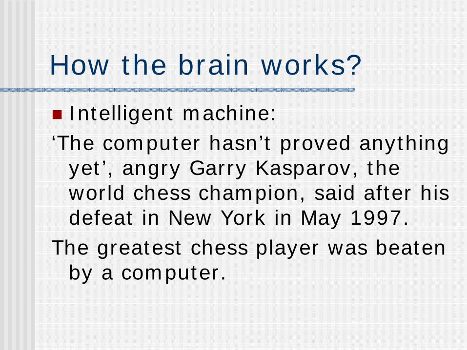
How the brain works?
Intelligent machine: ‘The computer hasn’t proved anything
yet’, angry Garry Kasparov, the world chess champion, said after his defeat in New York in May 1997.
The greatest chess player was beaten by a computer.
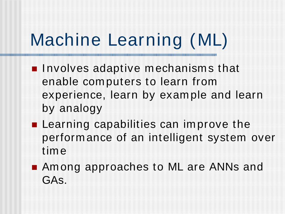
Machine Learning (ML)Involves adaptive mechanisms that enable computers to learn from experience, learn by example and learn by analogyLearning capabilities can improve the performance of an intelligent system over timeAmong approaches to ML are ANNs and GAs.
Soma Soma
Synapse
Synapse
Dendrites
Axon
Synapse
DendritesAxon
Biological Neural Network
Biological Neural Network-Typical Neuron-Dendrites
Nucleus

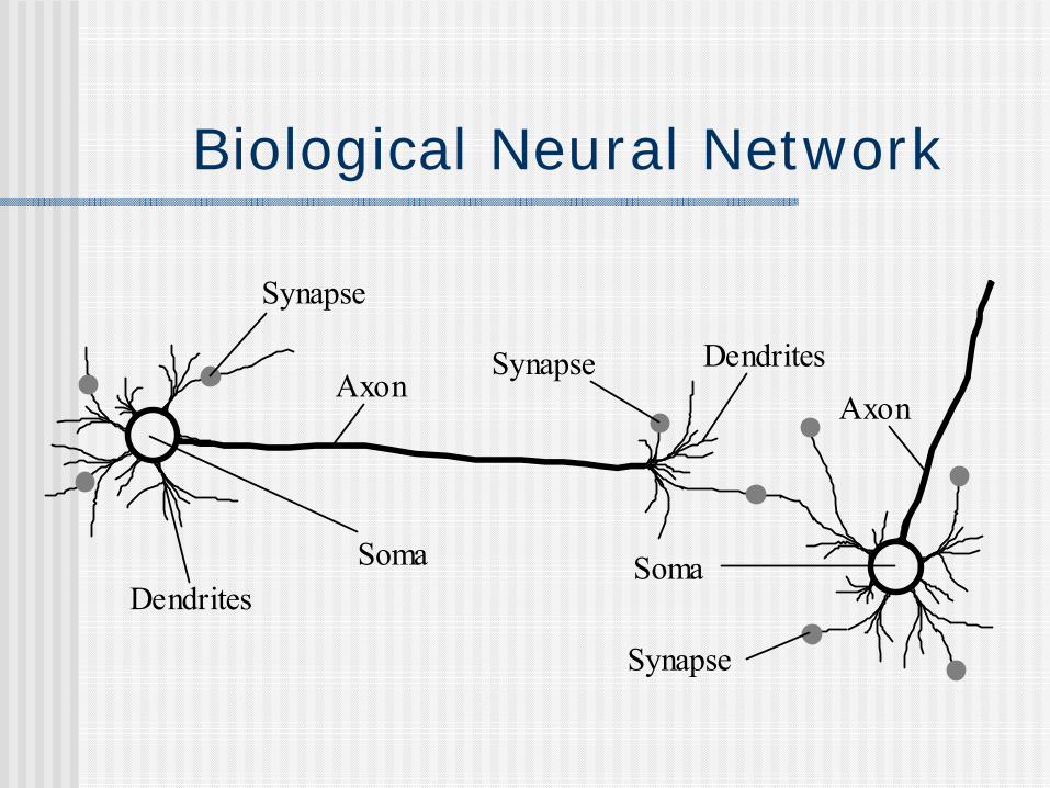
Neural NetworkA neural network can be defined as a model of reasoning based on the human brain. The brain consists of a densely interconnected set of nerve cells, or basic information-processing units, called neurons. The human brain incorporates nearly 10 billion neurons and 60 trillion connections, synapses, between them. By using multiple neurons simultaneously, the brain can perform its functions much faster than the fastest computers in existence today.

Neural Network
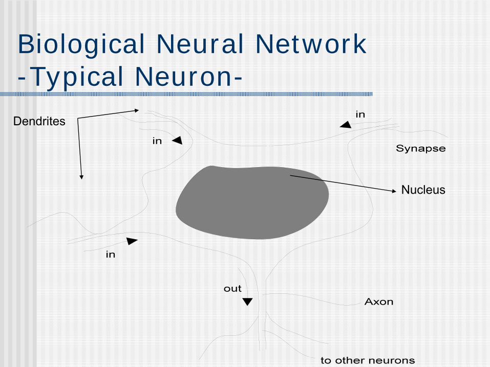
Each neuron has a very simple structure, but an army of such elements constitutes a tremendous processing power. A neuron consists of a cell body, soma, a number of fibers called dendrites, and a single long fiber called the axon.Our brain can be considered as a highly complex, non-linear and parallel information-processing system.

Information is stored and processed in a neural network simultaneously throughout the whole network, rather than at specific locations. In other words, in neural networks, both data and its processing are global rather than local.Learning is a fundamental and essential characteristic of biological neural networks. The ease with which they can learn led to attempts to emulate a biological neural network in a computer.
Neural Network

Artificial Neural Network-Simple Neuron-
●●●
Neuron Y
Y
Y
Y
Input Signals Weights Output Signals
w1
w2
wn
Raw data/outputs of other neurons
Final solution/input of other neurons
Computes activation level

Artificial Neural NetworkAn artificial neural network consists of a number of very simple processors, also called neurons, which are analogous to the biological neurons in the brain.
The neurons are connected by weighted links passing signals from one neuron to another.
The output signal is transmitted through the neuron’s outgoing connection. The outgoing connection splits into a number of branches that transmit the same signal. The outgoing branches terminate at the incoming connections of other neurons in the network.
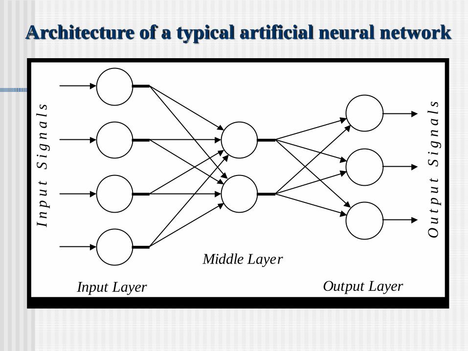
Architecture of a typical artificial neural network
Input Layer Output Layer
Middle Layer
I n p
u t
S i
g n
a l s
O u
t p
u t
S i
g n
a l s

Biological Neural Network Artificial Neural NetworkSomaDendriteAxonSynapse
NeuronInputOutputWeight
Analogy between biological and artificial neural networks

The neuron as a simple computing elementDiagram of a neuron
Neuron Y
Input Signals
x1
x2
xn
Output Signals
Y
Y
Y
w2
w1
wn
Weights

The neuron computes the weighted sum of the input signals and compares the result with a threshold value, θ. If the net input is less than the threshold, the neuron output is –1. But if the net input is greater than or equal to the threshold, the neuron becomes activated and its output attains a value +1.The neuron uses the following transfer or activationfunction:
This type of activation function is called a sign function.
∑=
=n
iiiwxX
1 ⎩⎨⎧
θ<−θ≥+
=XX
Y if ,1 if ,1

Activation functions of a neuron
Step function Sign function
+1
-10
+1
-10X
Y
X
Y+1
-10 X
Y
Sigmoid function
+1
-10 X
Y
Linear function
⎩⎨⎧
<≥
=0 if ,00 if ,1
XX
Ystep⎩⎨⎧
<−≥+
=0 if ,10 if ,1
XX
YsignX
sigmoid
eY
−+=
1
1 XYlinear=

Can a single neuron learn a task?
In 1958, Frank Rosenblatt introduced a training algorithm that provided the first procedure for training a simple ANN: a perceptron. The perceptron is the simplest form of a neural network. It consists of a single neuron with adjustable synaptic weights and a hard limiter.

Threshold
Inputs
x1
x2
OutputY∑
HardLimiter
w2
w1
LinearCombiner
θ
Single-layer two-input perceptron
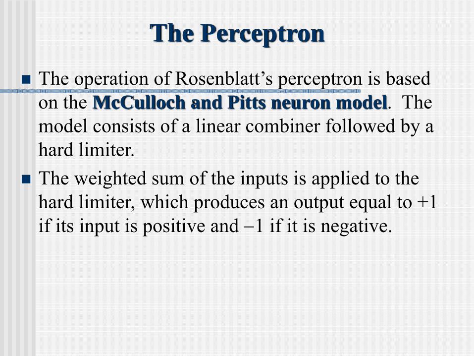
The Perceptron
The operation of Rosenblatt’s perceptron is based on the McCulloch and Pitts neuron model. The model consists of a linear combiner followed by a hard limiter. The weighted sum of the inputs is applied to the hard limiter, which produces an output equal to +1 if its input is positive and −1 if it is negative.

The aim of the perceptron is to classify inputs, x1, x2, . . ., xn, into one of two classes, say A1 and A2. In the case of an elementary perceptron, the n-dimensional space is divided by a hyperplane into two decision regions. The hyperplane is defined by the linearly separable function:
01
=θ−∑=
n
iiiwx

Linear separability in the perceptrons
x1
x2
Class A2
Class A1
1
2
x1w1 + x2w2 − θ = 0
(a) Two-input perceptron. (b) Three-input perceptron.
x2
x1
x3x1w1 + x2w2 + x3w3 − θ = 0
1 2

Solving OR..AND problem0 or 0 = 00 or 1=11 or 0 = 11 or 1 =1X1 or x2 = y
0 and 0 = 00 and 1= 01 and 0 = 01 and 1 =1X1 and x2 =y
This is done by making small adjustments in the weights to reduce the difference between the actual/estimated and desired/target outputs of the perceptron. The initial weights are randomly assigned, usually in the range [−0.5, 0.5], and then updated to obtain the output consistent with the training examples.
How does the perceptron learn its classification tasks?
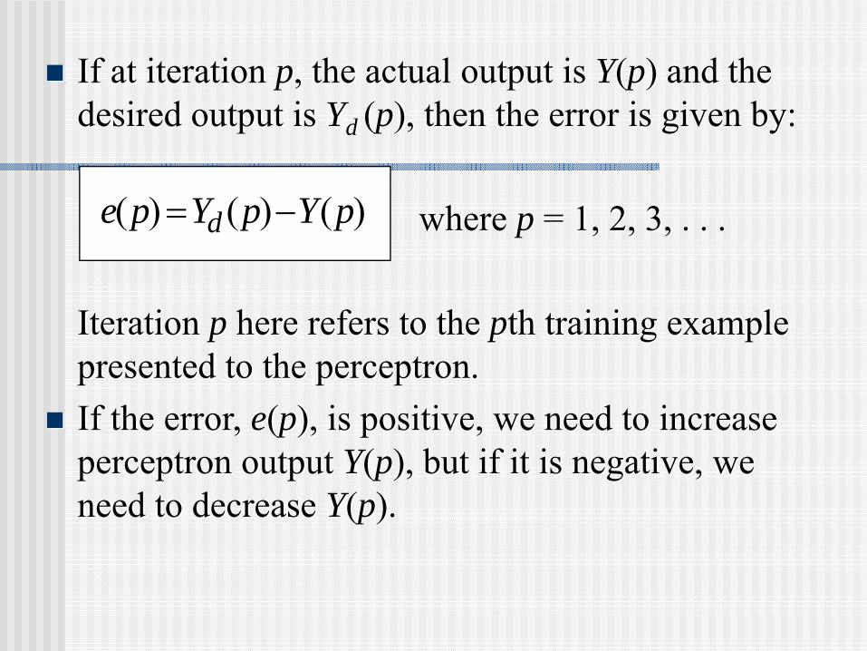
If at iteration p, the actual output is Y(p) and the desired output is Yd (p), then the error is given by:
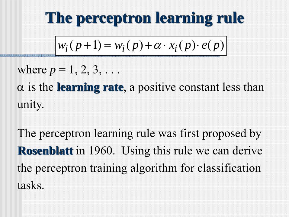
where p = 1, 2, 3, . . .
Iteration p here refers to the pth training example presented to the perceptron.If the error, e(p), is positive, we need to increase perceptron output Y(p), but if it is negative, we need to decrease Y(p).
)()()( pYpYpe d −=
The perceptron learning rule
where p = 1, 2, 3, . . .α is the learning rate, a positive constant less thanunity.
The perceptron learning rule was first proposed byRosenblatt in 1960. Using this rule we can derive the perceptron training algorithm for classification tasks.
)()()()1( pepxpwpw iii ⋅⋅+=+ α
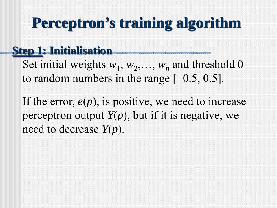
Step 1: InitialisationSet initial weights w1, w2,…, wn and threshold θto random numbers in the range [−0.5, 0.5].
If the error, e(p), is positive, we need to increase perceptron output Y(p), but if it is negative, we need to decrease Y(p).
Perceptron’s training algorithm
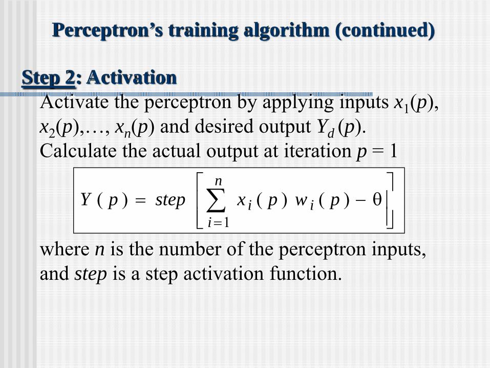
Step 2: ActivationActivate the perceptron by applying inputs x1(p), x2(p),…, xn(p) and desired output Yd (p). Calculate the actual output at iteration p = 1
where n is the number of the perceptron inputs, and step is a step activation function.
Perceptron’s training algorithm (continued)
⎥⎥⎦
⎤
⎢⎢⎣
⎡θ−= ∑
=
n
iii pwpxsteppY
1)( )()(
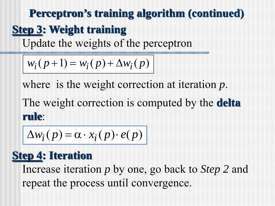
Step 3: Weight trainingUpdate the weights of the perceptron
where is the weight correction at iteration p.The weight correction is computed by the delta rule:
Step 4: IterationIncrease iteration p by one, go back to Step 2 and repeat the process until convergence.
)()()1( pwpwpw iii Δ+=+
Perceptron’s training algorithm (continued)
)()()( pepxpw ii ⋅⋅α=Δ

Example of perceptron learning: the logical operation ANDInputs
x1 x2
0011
0101
000
EpochDesiredoutput
Yd
1
Initialweights
w1 w2
1
0.30.30.30.2
−0.1−0.1−0.1−0.1
0010
Actualoutput
Y
Error
e00
−11
Finalweights
w1 w20.30.30.20.3
−0.1−0.1−0.1 0.0
0011
0101
000
2
1
0.30.30.30.2
0011
00−1
0
0.30.30.20.2
0.0 0.0
0.0 0.0
0011
0101
000
3
1
0.20.20.20.1
0.0 0.0
0.0 0.0
0.0 0.0
0.0 0.0
0010
00
−11
0.20.20.10.2
0.0 0.0
0.0 0.1
0011
0101
000
4
1
0.20.20.20.1
0.1 0.1
0.1 0.1
0011
00
−10
0.20.20.10.1
0.1 0.1
0.1 0.1
0011
0101
000
5
1
0.10.10.10.1
0.1 0.1
0.1 0.1
0001
00
0
0.10.10.10.1
0.1 0.1
0.1 0.1
0
Threshold: θ = 0.2; learning rate:α = 0.1
Final Weightis used
in the next pattern p (each line)

Two-dimensional plots of basic logical operations
x1
x2
1
(a) AND (x1 ∩ x2)
1
x1
x2
1
1
(b) OR (x1 ∪ x2)
x1
x2
1
1
(c) Exclusive-OR(x1 ⊕ x2)
00 0
A perceptron can learn the operations AND and OR, but not Exclusive-OR.

Multilayer neural networksA multilayer perceptron is a feedforward neural network with one or more hidden layers. The network consists of an input layer of source neurons, at least one middle or hidden layer of computational neurons, and an output layer of computational neurons. The input signals are propagated in a forward direction on a layer-by-layer basis.
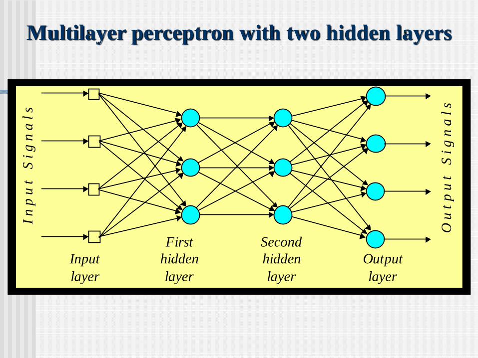
Multilayer perceptron with two hidden layers
Inputlayer
Firsthiddenlayer
Secondhiddenlayer
Outputlayer
O u
t p
u t
S i
g n
a l s
I n p
u t
S i
g n
a l s
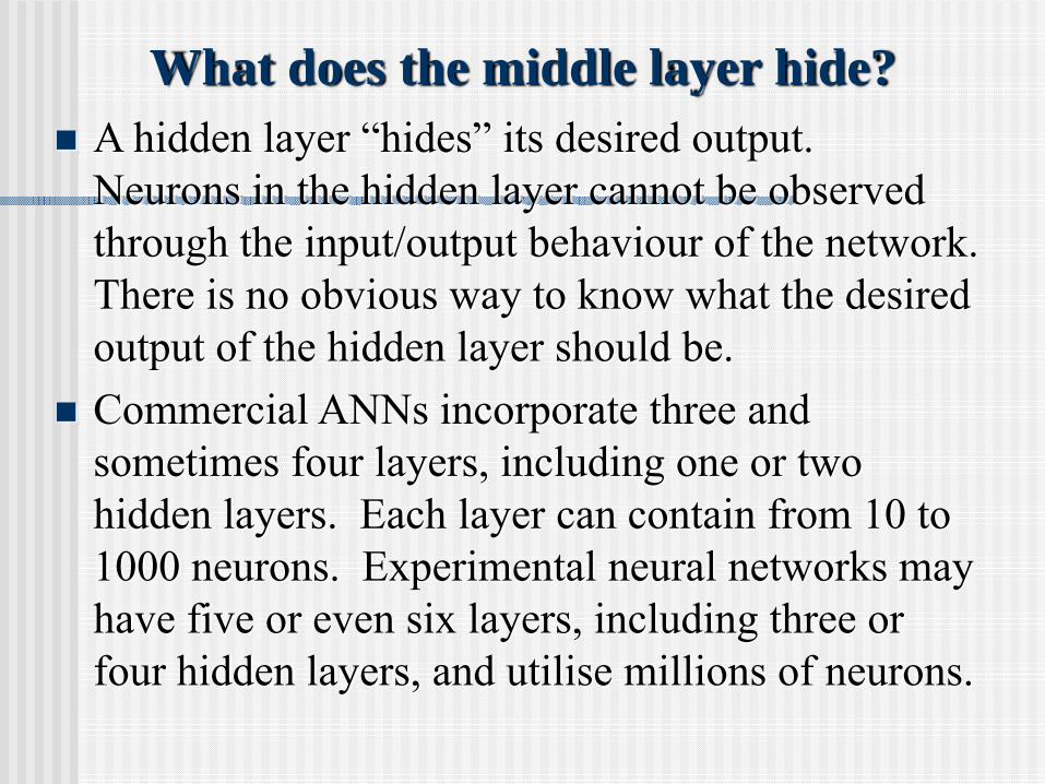
What does the middle layer hide?A hidden layer “hides” its desired output. Neurons in the hidden layer cannot be observed through the input/output behaviour of the network. There is no obvious way to know what the desired output of the hidden layer should be. Commercial ANNs incorporate three and sometimes four layers, including one or two hidden layers. Each layer can contain from 10 to 1000 neurons. Experimental neural networks may have five or even six layers, including three or four hidden layers, and utilise millions of neurons.
Back-propagation neural networkLearning in a multilayer network proceeds the same way as for a perceptron. A training set of input patterns is presented to the network. The network computes its output pattern, and if there is an error − or in other words a difference between actual and desired output patterns − the weights are adjusted to reduce this error.

In a back-propagation neural network, the learning algorithm has two phases. First, a training input pattern is presented to the network input layer. The network propagates the input pattern from layer to layer until the output pattern is generated by the output layer. If this pattern is different from the desired output, an error is calculated and then propagated backwards through the network from the output layer to the input layer. The weights are modified as the error is propagated.

Three-layer back-propagation neural network
Inputlayer
xi
x1
x2
xn
1
2
i
n
Outputlayer
1
2
k
l
yk
y1
y2
yl
Input signals
Error signals
wjk
Hiddenlayer
wij
1
2
j
m

Step 1: InitialisationSet all the weights and threshold levels of the network to random numbers uniformly distributed inside a small range:
where Fi is the total number of inputs of neuron iin the network. The weight initialisation is done on a neuron-by-neuron basis.
The back-propagation training algorithm
⎟⎟⎠
⎞⎜⎜⎝
⎛+−
ii FF4.2 ,4.2

Step 2: ActivationActivate the back-propagation neural network by applying inputs x1(p), x2(p),…, xn(p) and desired outputs yd,1(p), yd,2(p),…, yd,n(p).(a) Calculate the actual outputs of the neurons in the hidden layer:
where n is the number of inputs of neuron j in the hidden layer, and sigmoid is the sigmoid activation function.
⎥⎥⎦
⎤
⎢⎢⎣
⎡θ−⋅= ∑
=j
n
iijij pwpxsigmoidpy
1)()()(
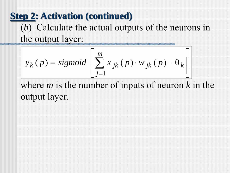
(b) Calculate the actual outputs of the neurons in the output layer:
where m is the number of inputs of neuron k in the output layer.
⎥⎥⎦
⎤
⎢⎢⎣
⎡θ−⋅= ∑
=k
m
jjkjkk pwpxsigmoidpy
1)()()(
Step 2: Activation (continued)

Step 3: Weight trainingUpdate the weights in the back-propagation network propagating backward the errors associated with output neurons.(a) Calculate the error gradient for the neurons in the output layer:
where
Calculate the weight corrections:
Update the weights at the output neurons:
[ ] )()(1)()( pepypyp kkkk ⋅−⋅=δ
)()()( , pypype kkdk −=
)()()( ppypw kjjk δα ⋅⋅=Δ
)()()1( pwpwpw jkjkjk Δ+=+
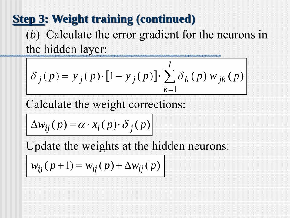
(b) Calculate the error gradient for the neurons in the hidden layer:
Calculate the weight corrections:
Update the weights at the hidden neurons:
)()()(1)()(1
][ p wppypyp jk
l
kkjjj ∑
=⋅−⋅= δδ
)()()( ppxpw jiij δα ⋅⋅=Δ
)()()1( pwpwpw ijijij Δ+=+
Step 3: Weight training (continued)
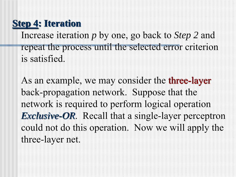
Step 4: IterationIncrease iteration p by one, go back to Step 2 and repeat the process until the selected error criterion is satisfied.
As an example, we may consider the three-layerback-propagation network. Suppose that the network is required to perform logical operation Exclusive-OR. Recall that a single-layer perceptron could not do this operation. Now we will apply the three-layer net.
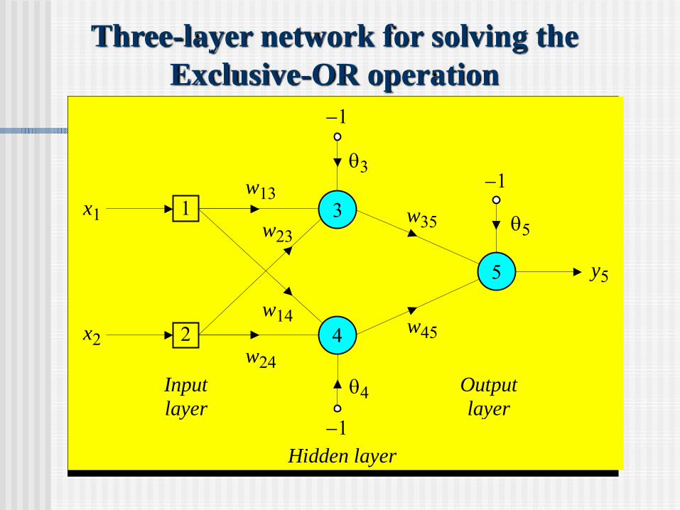
Three-layer network for solving the Exclusive-OR operation
y55
x1 31
x2
Input layer
Output layer
Hidden layer
42
θ3w13
w24
w23
w14
w35
w45
θ4
θ5
−1
−1
−1

The effect of the threshold applied to a neuron in the hidden or output layer is represented by its weight, θ, connected to a fixed input equal to −1.The initial weights and threshold levels are set randomly as follows:w13 = 0.5, w14 = 0.9, w23 = 0.4, w24 = 1.0, w35 = −1.2, w45 = 1.1, θ3 = 0.8, θ4 = −0.1 and θ5 = 0.3.

We consider a training set where inputs x1 and x2 are equal to 1 and desired output yd,5 is 0. The actual outputs of neurons 3 and 4 in the hidden layer are calculated as
[ ] 5250.01 /1)( )8.014.015.01(32321313 =+=θ−+= ⋅−⋅+⋅−ewxwx sigmoidy
[ ] 8808.01 /1)( )1.010.119.01(42421414 =+=θ−+= ⋅+⋅+⋅−ewxwx sigmoidy
Now the actual output of neuron 5 in the output layer is determined as:
Thus, the following error is obtained:
[ ] 5097.01 /1)( )3.011.18808.02.15250.0(54543535 =+=θ−+= ⋅−⋅+⋅−−ewywy sigmoidy
5097.05097.0055, −=−=−= yye d
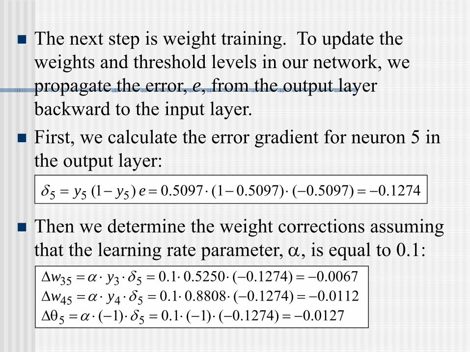
The next step is weight training. To update the weights and threshold levels in our network, we propagate the error, e, from the output layer backward to the input layer.First, we calculate the error gradient for neuron 5 in the output layer:
1274.05097).0( 0.5097)(1 0.5097)1( 555 −=−⋅−⋅=−= e y yδ
Then we determine the weight corrections assuming that the learning rate parameter, α, is equal to 0.1:
0112.0)1274.0(8808.01.05445 −=−⋅⋅=⋅⋅=Δ δα yw0067.0)1274.0(5250.01.05335 −=−⋅⋅=⋅⋅=Δ δα yw
0127.0)1274.0()1(1.0)1( 55 −=−⋅−⋅=⋅−⋅=θΔ δα
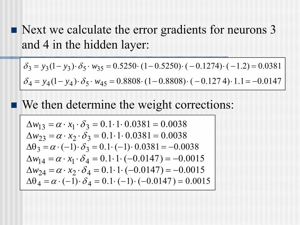
Next we calculate the error gradients for neurons 3 and 4 in the hidden layer:
We then determine the weight corrections:
0381.0)2.1 (0.1274) (0.5250)(1 0.5250)1( 355333 =−⋅−⋅−⋅=⋅⋅−= wyy δδ
0.0147.11 4) 0.127 ( 0.8808)(10.8808)1( 455444 −=⋅−⋅−⋅=⋅⋅−= wyy δδ
0038.00381.011.03113 =⋅⋅=⋅⋅=Δ δα xw0038.00381.011.03223 =⋅⋅=⋅⋅=Δ δα xw
0038.00381.0)1(1.0)1( 33 −=⋅−⋅=⋅−⋅=θΔ δα0015.0)0147.0(11.04114 −=−⋅⋅=⋅⋅=Δ δα xw0015.0)0147.0(11.04224 −=−⋅⋅=⋅⋅=Δ δα xw
0015.0)0147.0()1(1.0)1( 44 =−⋅−⋅=⋅−⋅=θΔ δα

At last, we update all weights and threshold:
5038.00038.05.0131313 =+=Δ+= www
8985.00015.09.0141414 =−=Δ+= www
4038.00038.04.0232323 =+=Δ+= www
9985.00015.00.1242424 =−=Δ+= www
2067.10067.02.1353535 −=−−=Δ+= www
0888.10112.01.1454545 =−=Δ+= www
7962.00038.08.0333 =−=θΔ+θ=θ
0985.00015.01.0444 −=+−=θΔ+θ=θ
3127.00127.03.0555 =+=θΔ+θ=θ
The training process is repeated until the sum of squared errors is less than 0.001.
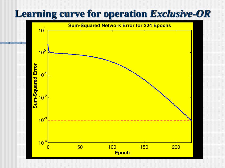
Learning curve for operation Exclusive-OR
0 50 100 150 200
101
Epoch
Su
m-S
qu
ared
Err
or
Sum-Squared Network Error for 224 Epochs
100
10-1
10-2
10-3
10-4

Final results of three-layer network learning
Inputs
x1 x2
1010
1100
011
Desiredoutput
yd
0
0.0155
Actualoutput
y5
Error
e
Sum ofsquarederrors
0.9849 0.9849 0.0175
−0.0155 0.0151 0.0151−0.0175
0.0010
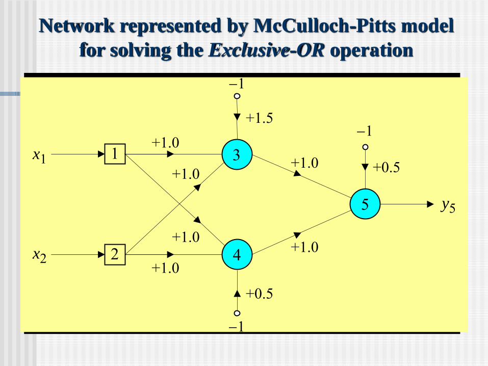
Network represented by McCulloch-Pitts model for solving the Exclusive-OR operation
y55
x1 31
x2 42
+1.0
−1
−1
−1+1.0
+1.0
+1.0
+1.5
+1.0
+1.0
+0.5
+0.5
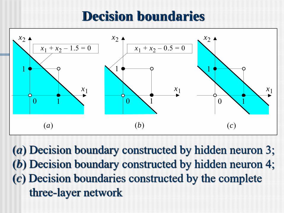
(a) Decision boundary constructed by hidden neuron 3;(b) Decision boundary constructed by hidden neuron 4; (c) Decision boundaries constructed by the complete
three-layer network
x1
x2
1
(a)
1
x2
1
1
(b)
00
x1 + x2 – 1.5 = 0 x1 + x2 – 0.5 = 0
x1 x1
x2
1
1
(c)
0
Decision boundaries