artificial neural network lecture 6- associative memories & discrete hopfield networks
TRANSCRIPT

1
CS407 Neural Computation
Lecture 6: Associative Memories and Discrete
Hopfield Network.
Lecturer: A/Prof. M. Bennamoun
2
AM and Discrete Hopfield Network.IntroductionBasic ConceptsLinear Associative Memory (Hetero-associative)Hopfield’s AutoassociativeMemoryPerformance Analysis for Recurrent AutoassociationMemoryReferences and suggested reading
IntroductionBasic ConceptsLinear Associative Memory (Hetero-associative)Hopfield’s AutoassociativeMemoryPerformance Analysis for Recurrent AutoassociationMemoryReferences and suggested reading
3
Fausett
Introduction…To a significant extent, learning is the process of forming associations between related patterns.Aristotle observed that human memory connects items (ideas, sensations, etc.) that are
– Similar– Contrary– Occur in close proximity (spatial)– Occur in close succession (temporal)
The patterns we associate together may be – of the same type or sensory modality (e.g. a visual
image may be associated with another visual image)– or of different types (e.g. a fragrance may be
associated with a visual image or a feeling).Memorization of a pattern (or a group of patterns) may be considered to be associating the pattern with itself.
4
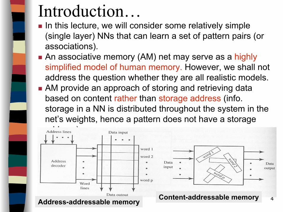
In this lecture, we will consider some relatively simple (single layer) NNs that can learn a set of pattern pairs (or associations). An associative memory (AM) net may serve as a highly simplified model of human memory. However, we shall not address the question whether they are all realistic models.AM provide an approach of storing and retrieving data based on content rather than storage address (info. storage in a NN is distributed throughout the system in the net’s weights, hence a pattern does not have a storage address)
Introduction…
Address-addressable memory Content-addressable memory
5
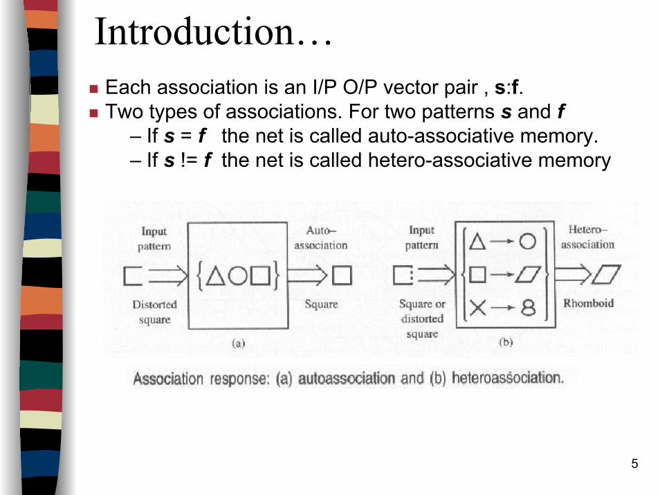
Introduction…Each association is an I/P O/P vector pair , s:f.Two types of associations. For two patterns s and f
– If s = f the net is called auto-associative memory.– If s != f the net is called hetero-associative memory
6
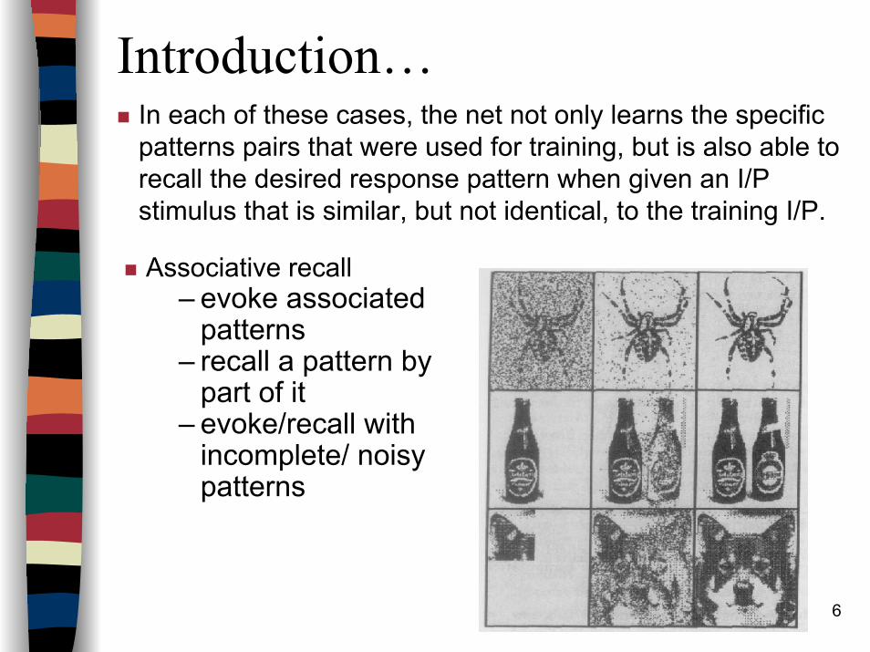
Introduction…In each of these cases, the net not only learns the specific patterns pairs that were used for training, but is also able to recall the desired response pattern when given an I/P stimulus that is similar, but not identical, to the training I/P.
Associative recall– evoke associated
patterns– recall a pattern by
part of it– evoke/recall with
incomplete/ noisy patterns
7
Introduction…Before training an AM NN, the original patterns must be converted to an appropriate representation for computation.
However, not all representations of the same pattern are equally powerful or efficient.
In a simple example, the original pattern might consist of “on” and “off” signals, and the conversion could be “on” +1 , “off” 0 (binary representation) or “on” +1, “off” -1 (bipolar representation).
Two common training methods for single layer nets are usually considered:
– Hebbian learning rule and its variations– gradient descent
8
Introduction…Architectures of NN associative memory may be
– Feedforward or– Recurrent (iterative).
On that basis we distinguish 4 types of AM:– Feedforward Hetero-associative– Feedforward Associative
– Iterative Hetero-associative– Iterative associative
A key question for all associative nets is – how many patterns can be stored before the net
starts to “forget” patterns it has learned previously (storage capacity)
9
IntroductionAssociative memories: Systems for associating the input patterns with the stored patterns (prototypes)– Dynamic systems with feedback networks– Static/Feedforward systems without
feedback networks
Information recording: A large set of patterns (the priori information) are stored (memorized)Information retrieval/recall: Stored prototypes are excited according to the input key patterns
10
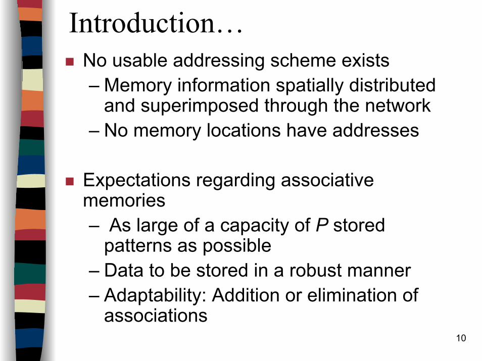
Introduction…No usable addressing scheme exists– Memory information spatially distributed
and superimposed through the network– No memory locations have addresses
Expectations regarding associative memories– As large of a capacity of P stored
patterns as possible– Data to be stored in a robust manner– Adaptability: Addition or elimination of
associations
11
AM and Discrete Hopfield Network.
IntroductionBasic ConceptsLinear Associative Memory (Hetero-associative)Hopfield’s AutoassociativeMemoryPerformance Analysis for Recurrent AutoassociationMemoryReferences and suggested reading
IntroductionBasic ConceptsLinear Associative Memory (Hetero-associative)Hopfield’s AutoassociativeMemoryPerformance Analysis for Recurrent AutoassociationMemoryReferences and suggested reading
12
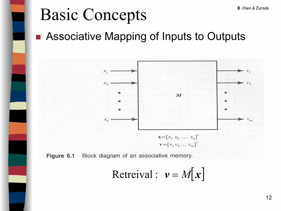
Basic Concepts B. Chen & Zurada
Associative Mapping of Inputs to Outputs
[ ]xv M= : Retreival
13
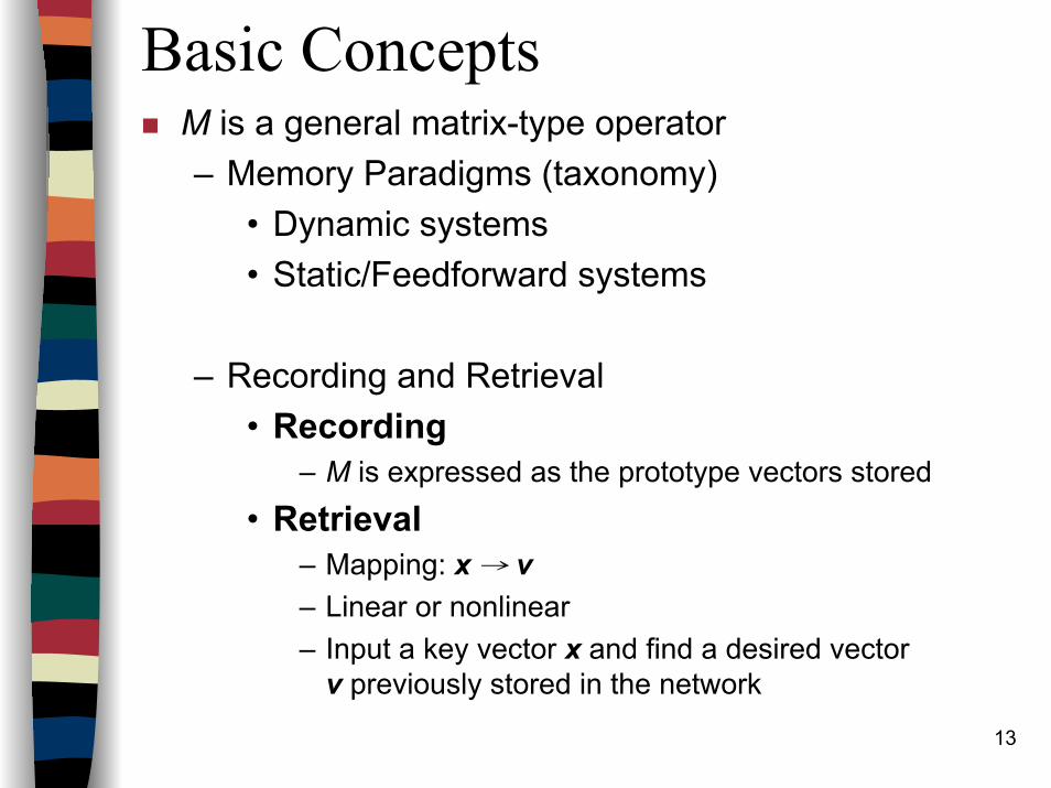
Basic ConceptsM is a general matrix-type operator– Memory Paradigms (taxonomy)
• Dynamic systems• Static/Feedforward systems
– Recording and Retrieval• Recording
– M is expressed as the prototype vectors stored
• Retrieval– Mapping: x → v– Linear or nonlinear – Input a key vector x and find a desired vector
v previously stored in the network
14
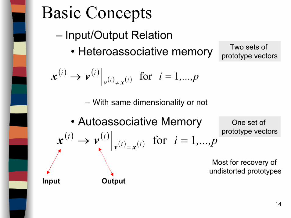
Basic Concepts– Input/Output Relation
• Heteroassociative memory
– With same dimensionality or not
• Autoassociative Memory
( ) ( )( ) ( ) ,...,piii
ii 1for =→≠ xv
vx
( ) ( )( ) ( ) ,...,piii
ii 1for =→= xv
vx
Two sets of prototype vectors
One set of prototype vectors
Output
Most for recovery of undistorted prototypes
Input
15
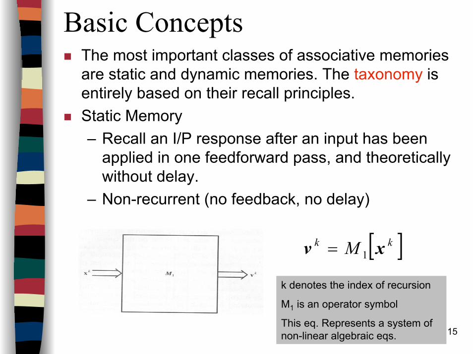
Basic ConceptsThe most important classes of associative memories are static and dynamic memories. The taxonomy is entirely based on their recall principles.Static Memory– Recall an I/P response after an input has been
applied in one feedforward pass, and theoretically without delay.
– Non-recurrent (no feedback, no delay)
[ ]kk M xv 1=
k denotes the index of recursion
M1 is an operator symbol
This eq. Represents a system of non-linear algebraic eqs.
16
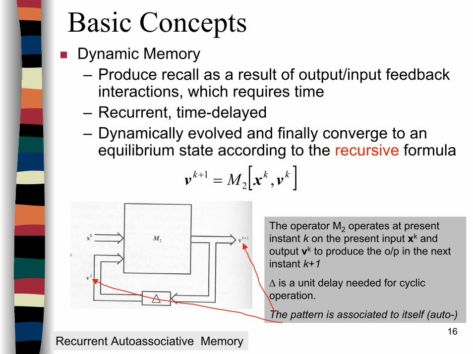
Basic ConceptsDynamic Memory– Produce recall as a result of output/input feedback
interactions, which requires time– Recurrent, time-delayed– Dynamically evolved and finally converge to an
equilibrium state according to the recursive formula
[ ] ,21 kkk M vxv =+
The operator M2 operates at present instant k on the present input xk and output vk to produce the o/p in the next instant k+1
∆ is a unit delay needed for cyclic operation.
The pattern is associated to itself (auto-)
Recurrent Autoassociative Memory
17
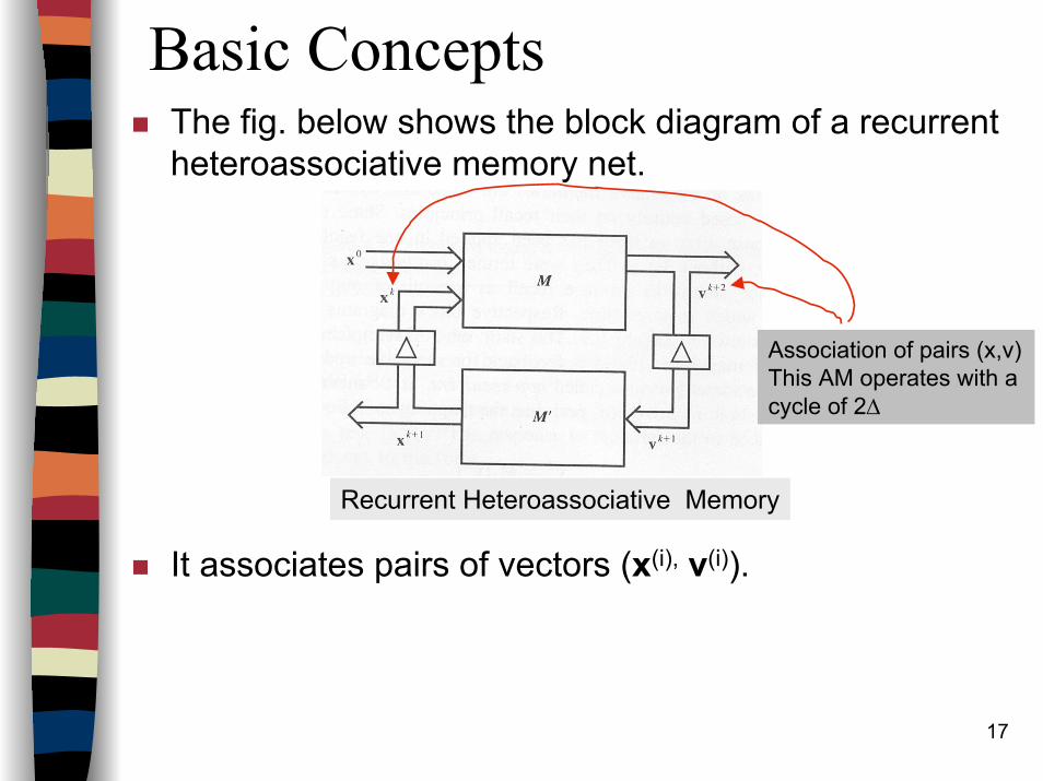
Basic ConceptsThe fig. below shows the block diagram of a recurrent heteroassociative memory net.
It associates pairs of vectors (x(i), v(i)).
Recurrent Heteroassociative Memory
Association of pairs (x,v)This AM operates with a cycle of 2∆
18
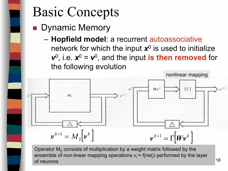
Basic ConceptsDynamic Memory– Hopfield model: a recurrent autoassociative
network for which the input x0 is used to initialize v0, i.e. x0 = v0, and the input is then removed for the following evolution
[ ] 21 kk M vv =+
nonlinear mapping
[ ] 1 kk Wvv Γ=+
Operator M2 consists of multiplication by a weight matrix followed by the ensemble of non-linear mapping operations vi = f(neti) performed by the layer of neurons
19
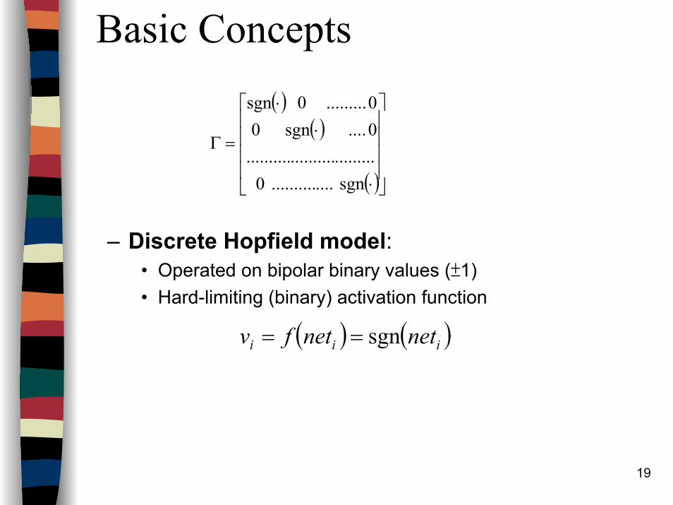
Basic Concepts( )
( )
( )
⋅
⋅⋅
=Γ
sgn .............. 0 .............................
0 .... sgn 0 0 ......... 0 sgn
– Discrete Hopfield model:• Operated on bipolar binary values (±1)• Hard-limiting (binary) activation function
( ) ( )iii netnetfv sgn==
20
Basic Concepts
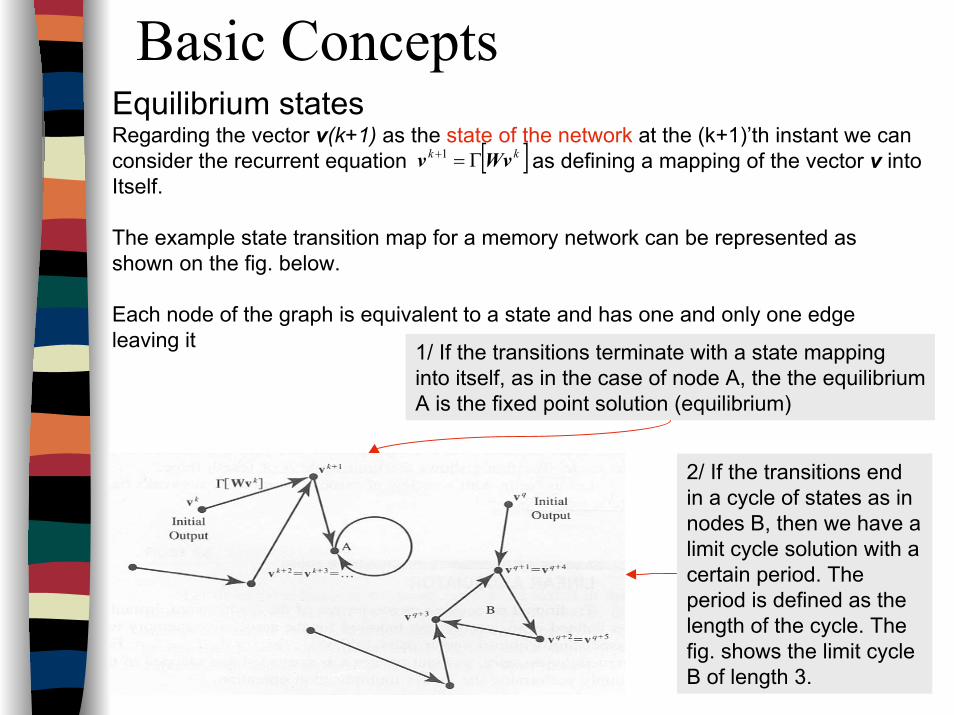
1/ If the transitions terminate with a state mapping into itself, as in the case of node A, the the equilibriumA is the fixed point solution (equilibrium)
Equilibrium statesRegarding the vector v(k+1) as the state of the network at the (k+1)’th instant we can consider the recurrent equation as defining a mapping of the vector v into Itself.
The example state transition map for a memory network can be represented as shown on the fig. below.
Each node of the graph is equivalent to a state and has one and only one edge leaving it
[ ] 1 kk Wvv Γ=+
2/ If the transitions end in a cycle of states as in nodes B, then we have a limit cycle solution with a certain period. The period is defined as the length of the cycle. The fig. shows the limit cycle B of length 3.
21
AM and Discrete Hopfield Network.IntroductionBasic ConceptsLinear Associative Memory (Hetero-associative)Hopfield’s AutoassociativeMemoryPerformance Analysis for Recurrent AutoassociationMemoryReferences and suggested reading
IntroductionBasic ConceptsLinear Associative Memory (Hetero-associative)Hopfield’s AutoassociativeMemoryPerformance Analysis for Recurrent AutoassociationMemoryReferences and suggested reading
22
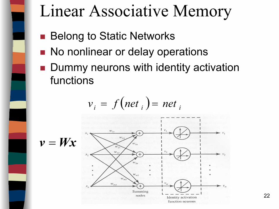
Linear Associative MemoryBelong to Static NetworksNo nonlinear or delay operationsDummy neurons with identity activation functions
( ) iii netnetfv ==
Wxv =
23
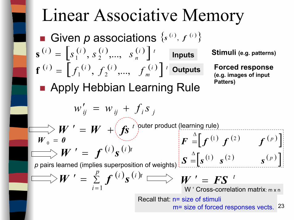
Linear Associative MemoryGiven p associations
Apply Hebbian Learning Rule
( ) ( ){ }ii fs ,
( ) ( ) ( ) ( )[ ]( ) ( ) ( ) ( )[ ] ti
miii
tin
iii
fff
sss
,...,,
,...,,
21
21
=
=
f
s
jiijij sfww +=′
Inputs
Outputs
Stimuli (e.g. patterns)
Forced response(e.g. images of input Patters)
tfsWW +=′
W ‘ Cross-correlation matrix: m x n
0W =0( ) ( )tii sfW =′
( ) ( )∑=
=′p
i
tii
1sfW
p pairs learned (implies superposition of weights)
tFSW =′
( ) ( ) ( )[ ]( ) ( ) ( )[ ]p
p
sssS
fffF
21
21
∆
∆
=
=
outer product (learning rule)
Recall that: n= size of stimuli m= size of forced responses vects.
24
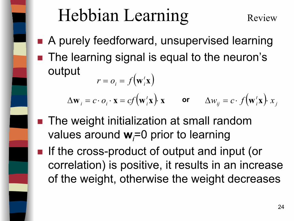
Hebbian Learning Review
A purely feedforward, unsupervised learningThe learning signal is equal to the neuron’s output
The weight initialization at small random values around wi=0 prior to learningIf the cross-product of output and input (or correlation) is positive, it results in an increase of the weight, otherwise the weight decreases
( )xw tii for ==
( ) xxwxw ⋅=⋅⋅=∆ tiii cfoc ( ) j
tiij xfcw ⋅⋅=∆ xwor
25
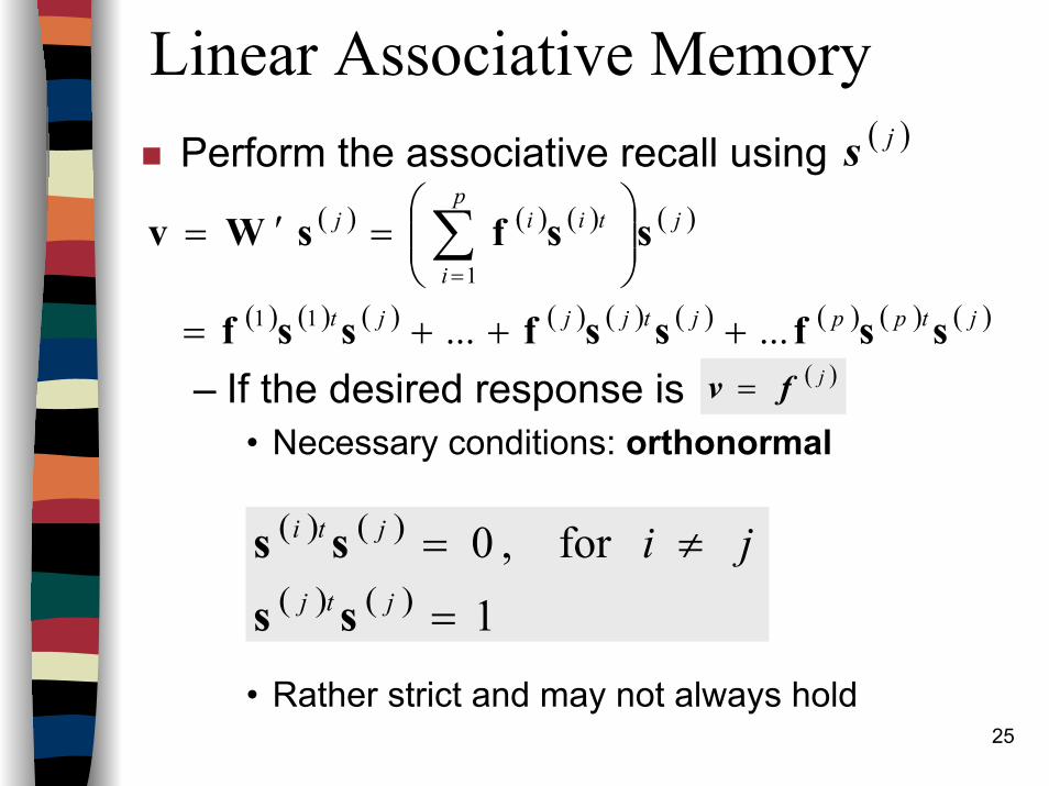
Linear Associative MemoryPerform the associative recall using
– If the desired response is• Necessary conditions: orthonormal
• Rather strict and may not always hold
( ) ( ) ( ) ( )
( ) ( ) ( ) ( ) ( ) ( ) ( ) ( ) ( )jtppjtjjjt
jp
i
tiij
ssfssfssf
ssfsWv
...... 11
1
+++=
=′= ∑
=
( )js
( )jfv =
( ) ( )
( ) ( ) 1for ,0
=
≠=jtj
jti j issss
26
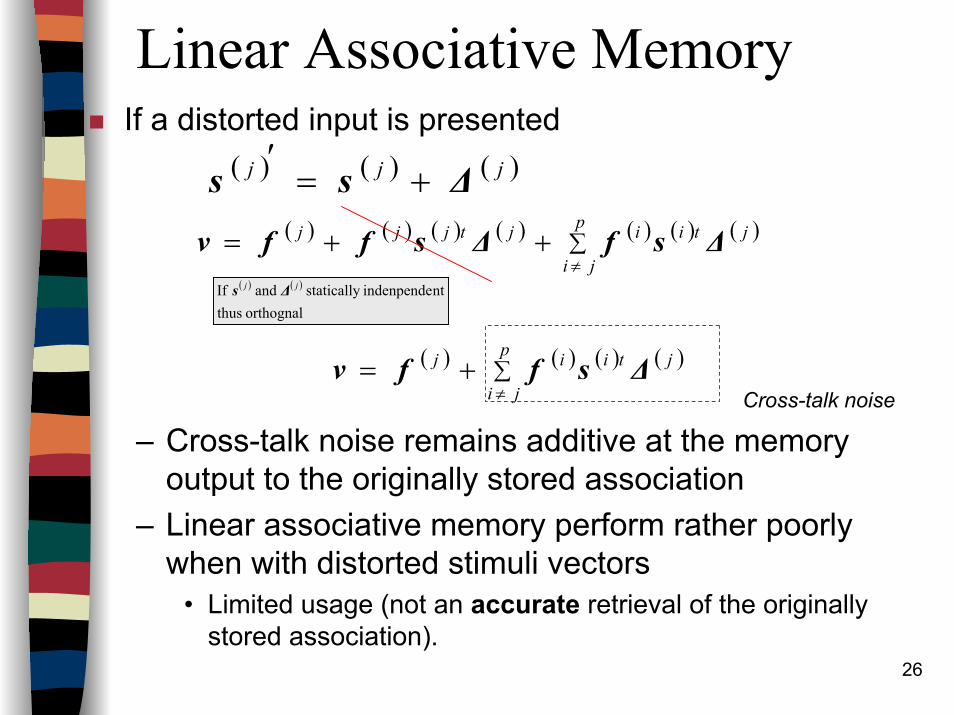
Linear Associative MemoryIf a distorted input is presented
– Cross-talk noise remains additive at the memory output to the originally stored association
– Linear associative memory perform rather poorly when with distorted stimuli vectors
• Limited usage (not an accurate retrieval of the originally stored association).
( ) ( ) ( )jjj ∆ss +=′
( ) ( ) ( ) ( ) ( ) ( ) ( )∑≠
++=p
ji
jtiijtjjj ∆sf∆sffv
( ) ( ) ( ) ( )∑≠
+=p
ji
jtiij ∆sffv
( ) ( )
orthognal thusntindenpende statically and If jj ∆s
Cross-talk noise
27
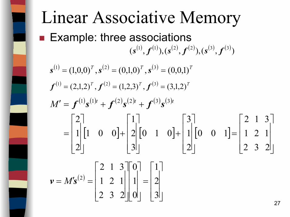
Linear Associative MemoryExample: three associations
( ) ( ) ( ) ( ) ( ) ( )),(),,(),,( 332211 fsfsfs
( ) ( ) ( ) TTT )1,0,0(,)0,1,0(,)0,0,1( 321 === sss( ) ( ) ( ) TTT )2,1,3(,)3,2,1(,)2,1,2( 321 === fff
( ) ( ) ( ) ( ) ( ) ( )
[ ] [ ] [ ]
=
+
+
=
++=′
2 3 21 2 13 1 2
100213
010321
001212
332211 tttM sfsfsf
( )
=
=′=
321
010
2 3 21 2 13 1 2
2sv M
28
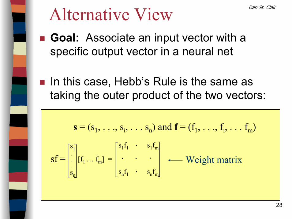
Alternative View Dan St. Clair
Goal: Associate an input vector with a specific output vector in a neural net
In this case, Hebb’s Rule is the same as taking the outer product of the two vectors:
s = (s1, . . ., si, . . . sn) and f = (f1, . . ., fi, . . . fm)
sf = [f1 … fm] =
s1
sn
.
.
.
s1f1 s1fm
snf1 snfm
..
.
. . Weight matrix
29
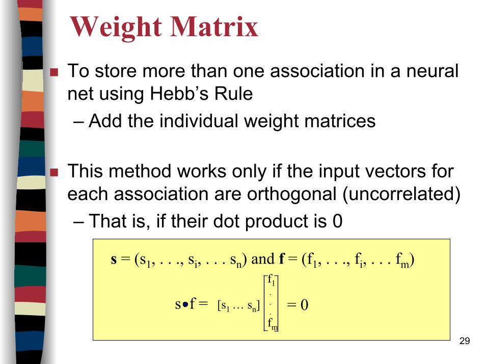
Weight MatrixTo store more than one association in a neural net using Hebb’s Rule– Add the individual weight matrices
This method works only if the input vectors for each association are orthogonal (uncorrelated)– That is, if their dot product is 0
s = (s1, . . ., si, . . . sn) and f = (f1, . . ., fi, . . . fm)
s f = [s1 … sn]
f1
fm
.
.
. = 0
30
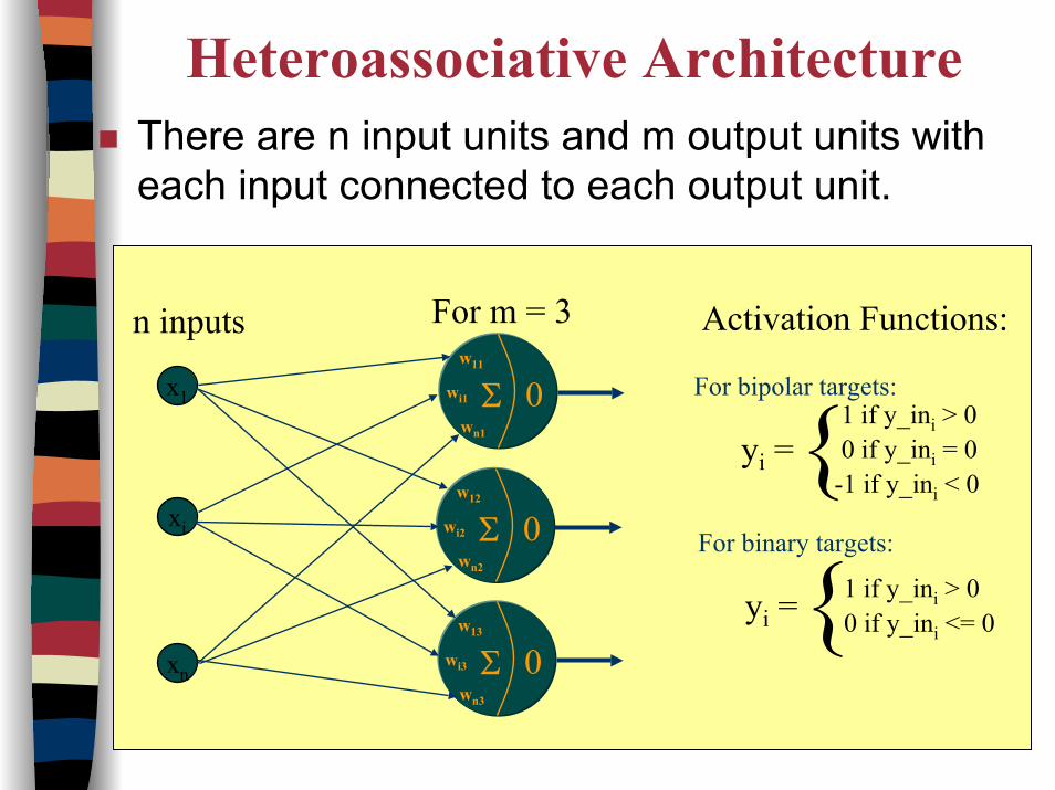
Heteroassociative ArchitectureThere are n input units and m output units with each input connected to each output unit.
0wi1
wn1
Σw11
0wi2
wn2
Σw12
0wi3
wn3
Σw13
For m = 3
x1
xi
xn
n inputs Activation Functions:
For bipolar targets:
yi = 1 if y_ini > 00 if y_ini = 0
-1 if y_ini < 0{For binary targets:
yi = 1 if y_ini > 00 if y_ini <= 0{
31
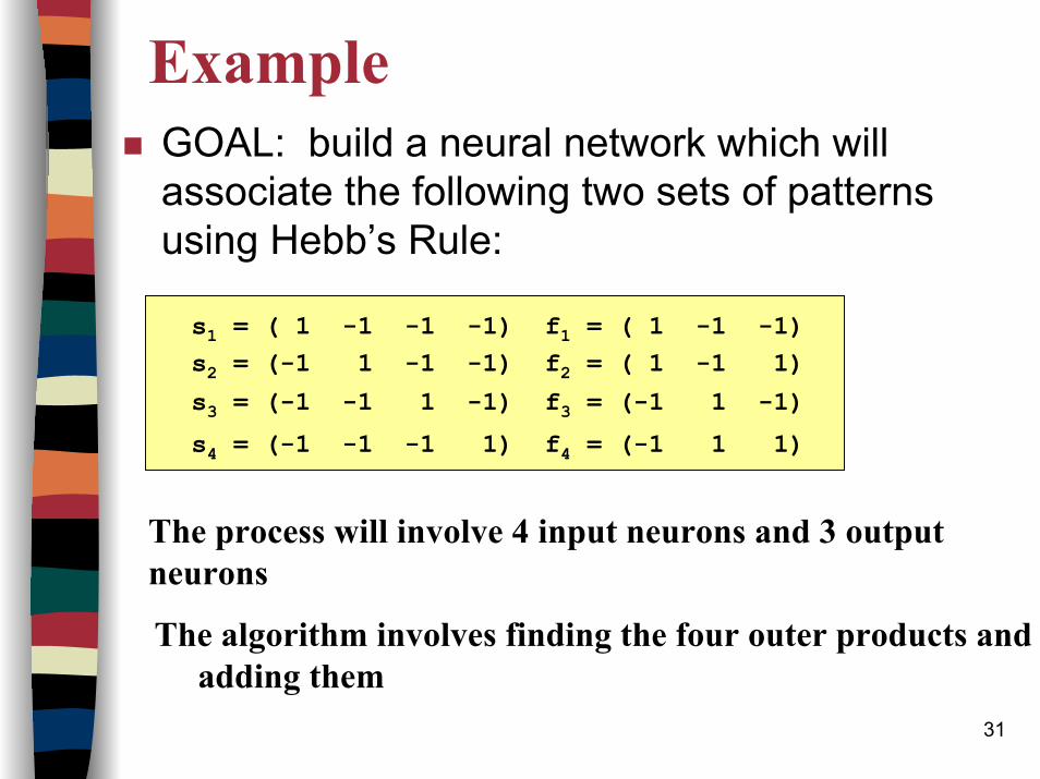
ExampleGOAL: build a neural network which will associate the following two sets of patterns using Hebb’s Rule:
s1 = ( 1 -1 -1 -1) f1 = ( 1 -1 -1)s2 = (-1 1 -1 -1) f2 = ( 1 -1 1)s3 = (-1 -1 1 -1) f3 = (-1 1 -1)s4 = (-1 -1 -1 1) f4 = (-1 1 1)
The process will involve 4 input neurons and 3 output neurons
The algorithm involves finding the four outer products andadding them
32
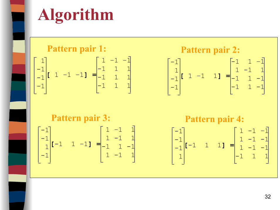
Algorithm
1-1-1-1
[ 1 –1 –1] = 1 –1 –1-1 1 1-1 1 1-1 1 1
Pattern pair 1:-11-1-1
[ 1 –1 1] = -1 1 –11 -1 1-1 1 -1-1 1 -1
Pattern pair 2:
-1-11-1
[-1 1 –1] = 1 –1 11 -1 1-1 1 -11 -1 1
Pattern pair 3:-1-1-11[-1 1 1] =
1 -1 –11 -1 -11 -1 -1-1 1 1
Pattern pair 4:
33
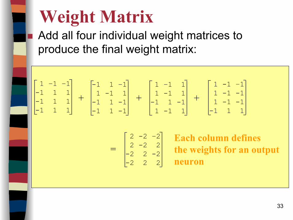
Weight MatrixAdd all four individual weight matrices to produce the final weight matrix:
1 –1 –1-1 1 1-1 1 1-1 1 1
-1 1 –11 -1 1-1 1 -1-1 1 -1
1 –1 11 -1 1-1 1 -11 -1 1
1 -1 –11 -1 -11 -1 -1-1 1 1
+ + +
2 -2 –22 -2 2-2 2 -2-2 2 2
=Each column definesthe weights for an outputneuron
34
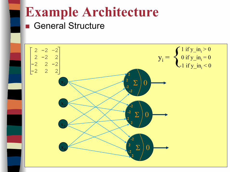
Example ArchitectureGeneral Structure
x1
x2
x4
x3
02
-2Σ
2
-2
0-2
2Σ
-2
2
02
-2Σ
-2
2
yi = 1 if y_ini > 00 if y_ini = 0
-1 if y_ini < 0{2 -2 –2
2 -2 2-2 2 -2-2 2 2
35
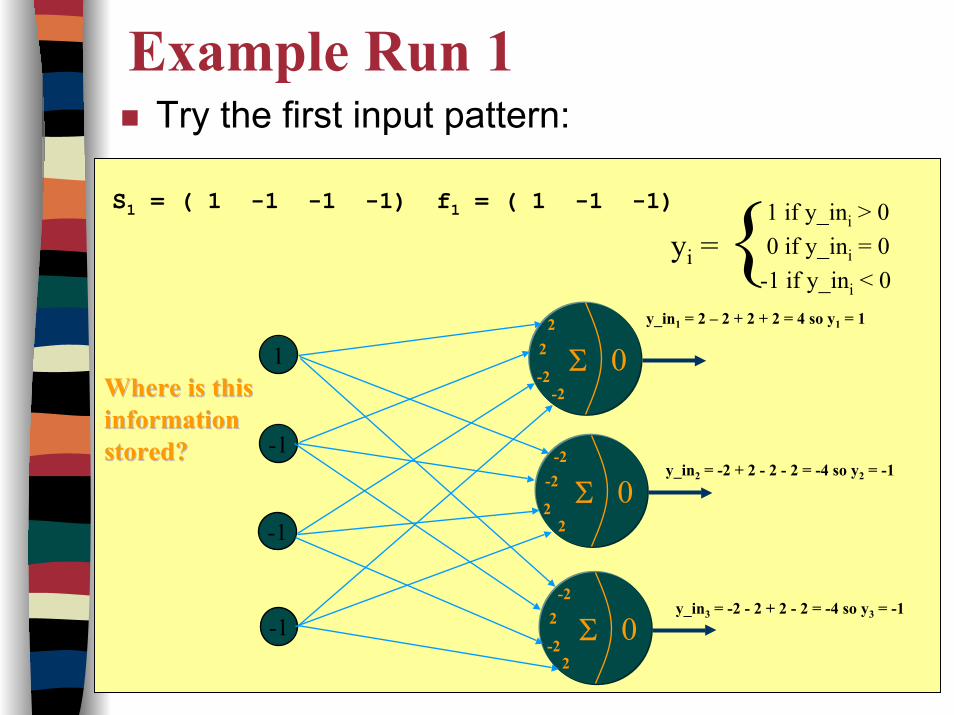
Example Run 1Try the first input pattern:
1
-1
-1
-1
02
-2Σ
2
-2
0-2
2Σ
-2
2
02
-2Σ
-2
2
yi = 1 if y_ini > 00 if y_ini = 0
-1 if y_ini < 0{
y_in1 = 2 – 2 + 2 + 2 = 4 so y1 = 1
y_in2 = -2 + 2 - 2 - 2 = -4 so y2 = -1
y_in3 = -2 - 2 + 2 - 2 = -4 so y3 = -1
S1 = ( 1 -1 -1 -1) f1 = ( 1 -1 -1)
Where is thisWhere is thisinformationinformationstored?stored?
36
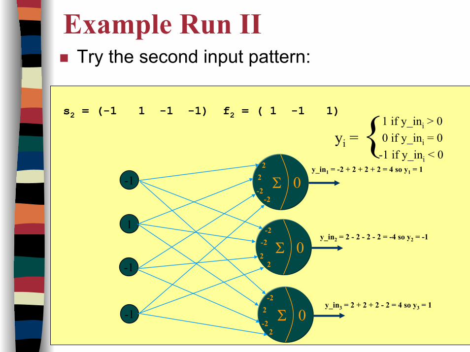
Example Run IITry the second input pattern:
s2 = (-1 1 -1 -1) f2 = ( 1 -1 1)
-1
1
-1
-1
02
-2Σ
2
-2
0-2
2Σ
-2
2
02
-2Σ
-2
2
yi = 1 if y_ini > 00 if y_ini = 0
-1 if y_ini < 0{
y_in1 = -2 + 2 + 2 + 2 = 4 so y1 = 1
y_in2 = 2 - 2 - 2 - 2 = -4 so y2 = -1
y_in3 = 2 + 2 + 2 - 2 = 4 so y3 = 1
37
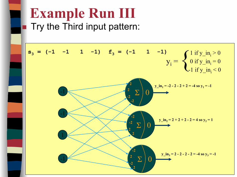
Example Run IIITry the Third input pattern:
s3 = (-1 -1 1 -1) f3 = (-1 1 -1)
-1
-1
-1
1
02
-2Σ
2
-2
0-2
2Σ
-2
2
02
-2Σ
-2
2
yi = 1 if y_ini > 00 if y_ini = 0
-1 if y_ini < 0{
y_in1 = -2 - 2 - 2 + 2 = -4 so y1 = -1
y_in2 = 2 + 2 + 2 - 2 = 4 so y2 = 1
y_in3 = 2 - 2 - 2 - 2 = -4 so y3 = -1
38
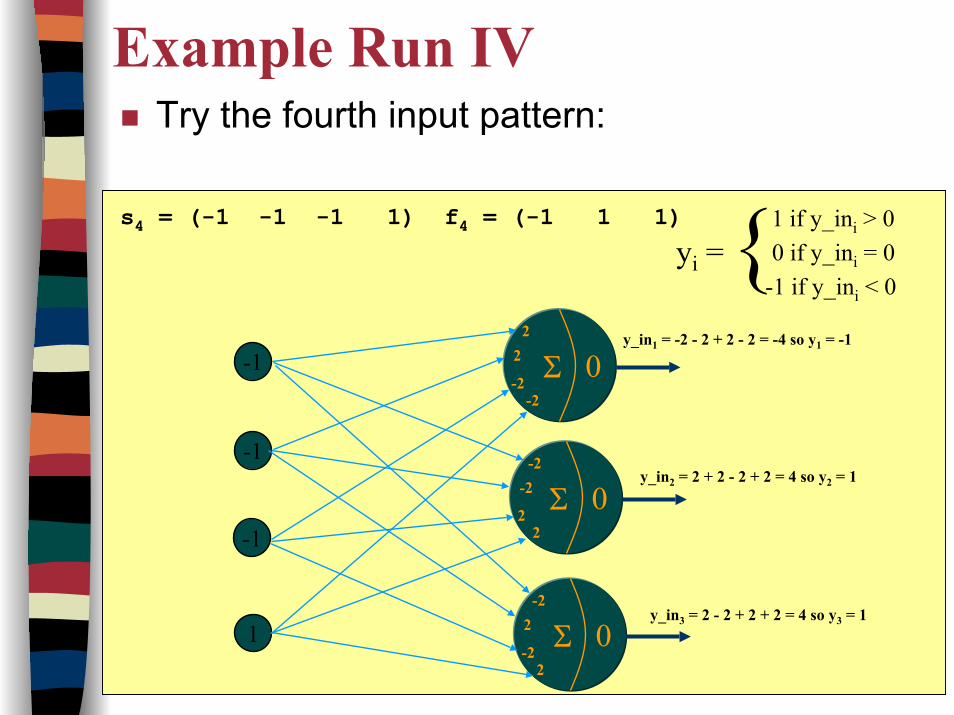
Example Run IVTry the fourth input pattern:
s4 = (-1 -1 -1 1) f4 = (-1 1 1)
-1
-1
1
-1
02
-2Σ
2
-2
0-2
2Σ
-2
2
02
-2Σ
-2
2
yi = 1 if y_ini > 00 if y_ini = 0
-1 if y_ini < 0{
y_in1 = -2 - 2 + 2 - 2 = -4 so y1 = -1
y_in2 = 2 + 2 - 2 + 2 = 4 so y2 = 1
y_in3 = 2 - 2 + 2 + 2 = 4 so y3 = 1
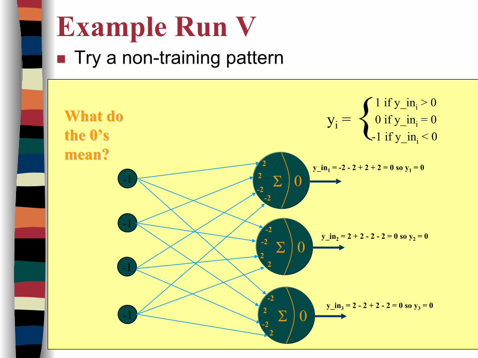
39
Example Run VTry a non-training pattern
-1
-1
-1
-1
02
-2Σ
2
-2
0-2
2Σ
-2
2
02
-2Σ
-2
2
yi = 1 if y_ini > 00 if y_ini = 0
-1 if y_ini < 0{
y_in1 = -2 - 2 + 2 + 2 = 0 so y1 = 0
y_in2 = 2 + 2 - 2 - 2 = 0 so y2 = 0
y_in3 = 2 - 2 + 2 - 2 = 0 so y3 = 0
What doWhat dothe 0’sthe 0’smean?mean?
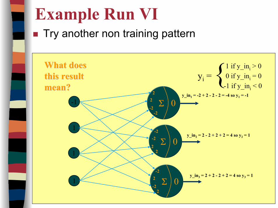
40
Example Run VITry another non training pattern
-1
1
1
1
02
-2Σ
2
-2
0-2
2Σ
-2
2
02
-2Σ
-2
2
yi = 1 if y_ini > 00 if y_ini = 0
-1 if y_ini < 0{
y_in1 = -2 + 2 - 2 - 2 = -4 so y1 = -1
y_in2 = 2 - 2 + 2 + 2 = 4 so y2 = 1
y_in3 = 2 + 2 - 2 + 2 = 4 so y3 = 1
What doesWhat doesthis resultthis resultmean?mean?
41
AM and Discrete Hopfield Network.IntroductionBasic ConceptsLinear Associative Memory (Hetero-associative)Hopfield’s AutoassociativeMemoryPerformance Analysis for Recurrent AutoassociationMemoryReferences and suggested reading
IntroductionBasic ConceptsLinear Associative Memory (Hetero-associative)Hopfield’s AutoassociativeMemoryPerformance Analysis for Recurrent AutoassociationMemoryReferences and suggested reading
42
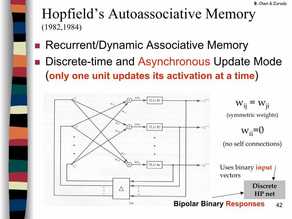
Hopfield’s Autoassociative Memory (1982,1984)
B. Chen & Zurada
Recurrent/Dynamic Associative MemoryDiscrete-time and Asynchronous Update Mode (only one unit updates its activation at a time)
Bipolar Binary Responses
wij = wji(symmetric weights)
wii=0 (no self connections)
Uses binary inputvectors
Discrete HP net
43
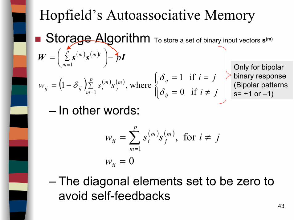
Hopfield’s Autoassociative MemoryStorage Algorithm To store a set of binary input vectors s(m)
– In other words:
– The diagonal elements set to be zero to avoid self-feedbacks
( ) ( )
( ) ( ) ( )
≠=
==−=
−
=
∑
∑
=
=
ji
jissw
p
ij
ijp
m
mj
miijij
p
m
tmm
if 0
if 1 where,1
1
1
δ
δδ
IssWOnly for bipolarbinary response(Bipolar patterns s= +1 or –1)
( ) ( )
0
for ,1
=
≠= ∑=
ii
p
m
mj
miij
w
jissw
44
Hopfield’s Autoassociative Memory– The matrix only represents the correlation
terms among the vector entries– Invariant with respect to the sequence of
storing patterns– Additional autoassociations can be added
at any time by superimposition– autoassociations can also be removed
45
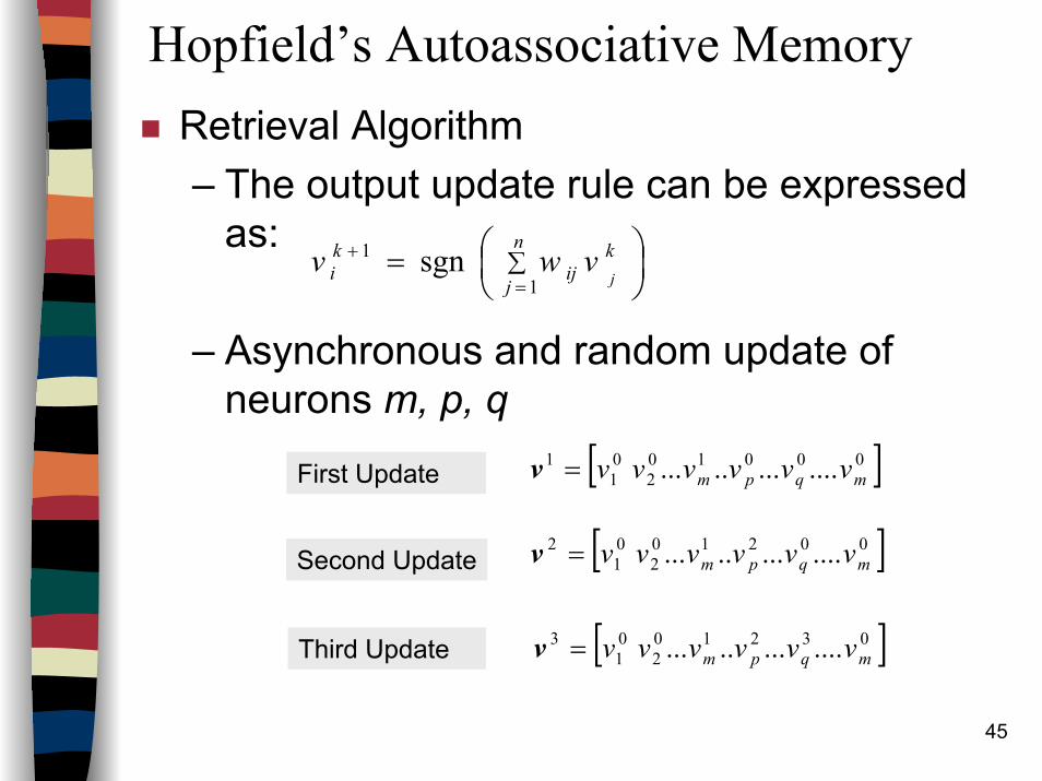
Hopfield’s Autoassociative MemoryRetrieval Algorithm– The output update rule can be expressed
as:
– Asynchronous and random update of neurons m, p, q
sgn1
1
= ∑
=
+ n
j
kij
ki j
vwv
[ ]002102
01
2 ............ mqpm vvvvvv=v
[ ]000102
01
1 ............ mqpm vvvvvv=v
[ ]032102
01
3 ............ mqpm vvvvvv=v
First Update
Third Update
Second Update
46
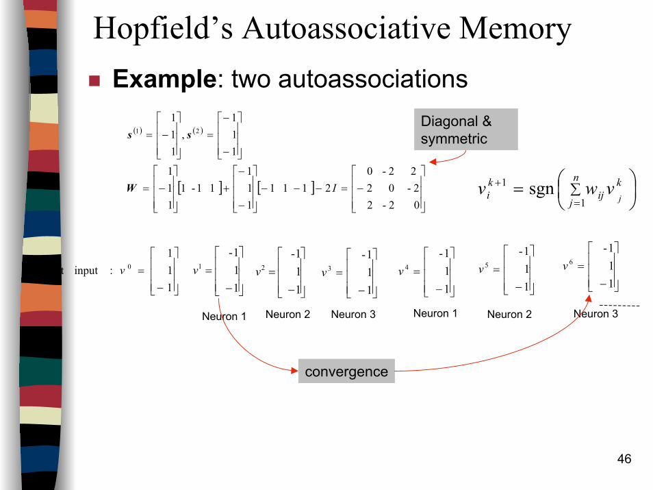
Hopfield’s Autoassociative MemoryExample: two autoassociations
( ) ( )
[ ] [ ]
−=−−−
−
−+
−=
−
−=
−=
0 2- 2 2- 0 2
2 2- 0 2 1 1 1
11 1
1 1- 11 11
11 1
,1 11
21
IW
ss
= ∑
=
+ n
j
kij
ki j
vwv1
1 sgn
Diagonal & symmetric
−=
1 1 1-
1v
Neuron 1
−=
1 1 1-
2v
−=
1 1 1-
4v
−=
1 1 1-
3v
−=
1 1 1-
5v
−=
1 1 1-
6v
Neuron 2 Neuron 3 Neuron 1 Neuron 2 Neuron 3
convergence
−=
11 1
:inputTest 0v
47
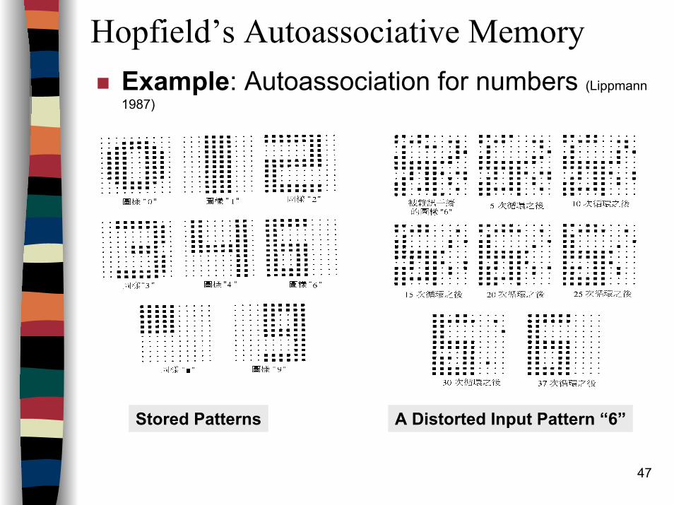
Hopfield’s Autoassociative MemoryExample: Autoassociation for numbers (Lippmann1987)
Stored Patterns A Distorted Input Pattern “6”
48
Hopfield’s Autoassociative Memory
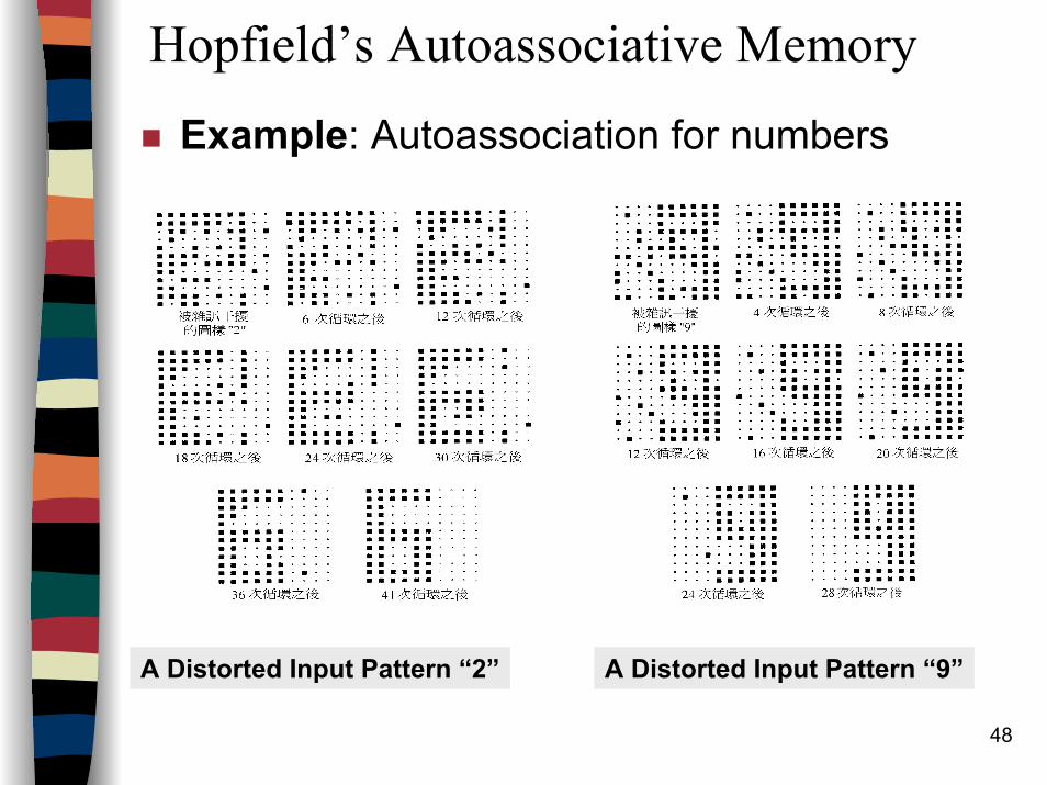
Example: Autoassociation for numbers
A Distorted Input Pattern “2” A Distorted Input Pattern “9”
49
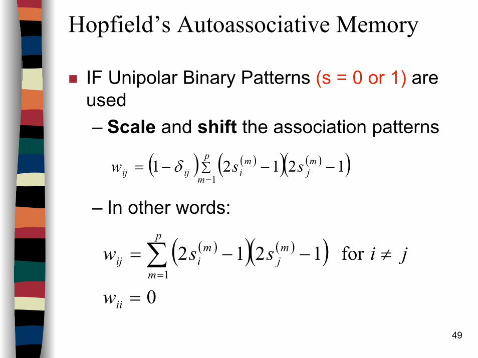
Hopfield’s Autoassociative Memory
IF Unipolar Binary Patterns (s = 0 or 1) are used– Scale and shift the association patterns
– In other words:
( ) ( )( ) ( )( )∑=
−−−=p
m
mj
miijij ssw
112121 δ
( )( ) ( )( )0
for 12121
=
≠−−= ∑=
ii
p
m
mj
miij
w
jissw
50
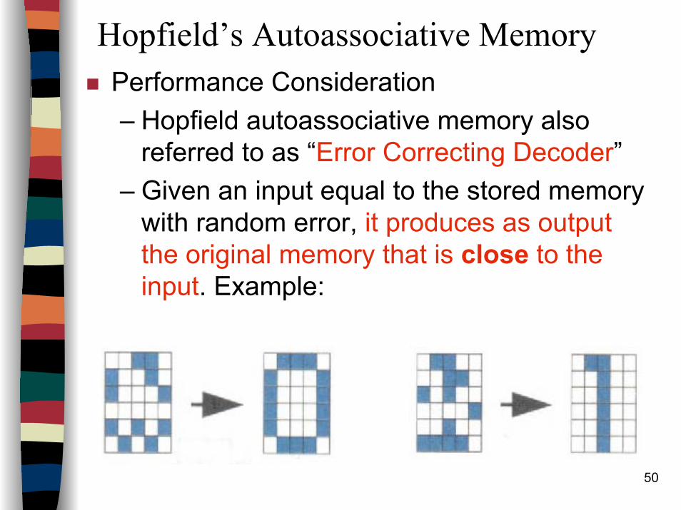
Hopfield’s Autoassociative MemoryPerformance Consideration– Hopfield autoassociative memory also
referred to as “Error Correcting Decoder”– Given an input equal to the stored memory
with random error, it produces as output the original memory that is close to the input. Example:
51
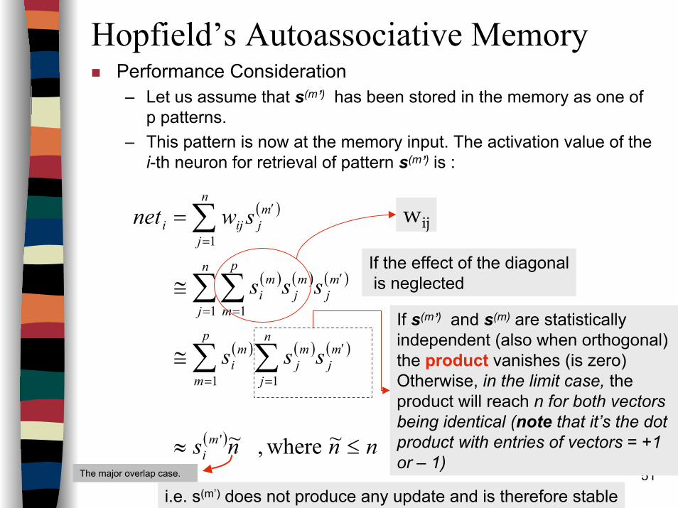
Hopfield’s Autoassociative MemoryPerformance Consideration– Let us assume that s(m’) has been stored in the memory as one of
p patterns.– This pattern is now at the memory input. The activation value of the
i-th neuron for retrieval of pattern s(m’) is :
( )
( ) ( ) ( )
( ) ( ) ( )
( ) nnns
sss
sss
swnet
mi
p
m
n
j
mj
mj
mi
n
j
p
m
mj
mj
mi
n
j
mjiji
≤≈
≅
≅
=
∑ ∑
∑∑
∑
= =
′
= =
′
=
′
~ where, ~
'
1 1
1 1
1
If s(m’) and s(m) are statisticallyindependent (also when orthogonal) the product vanishes (is zero)Otherwise, in the limit case, the product will reach n for both vectors being identical (note that it’s the dot product with entries of vectors = +1 or – 1)
If the effect of the diagonalis neglected
wij
The major overlap case.
i.e. s(m’) does not produce any update and is therefore stable
52
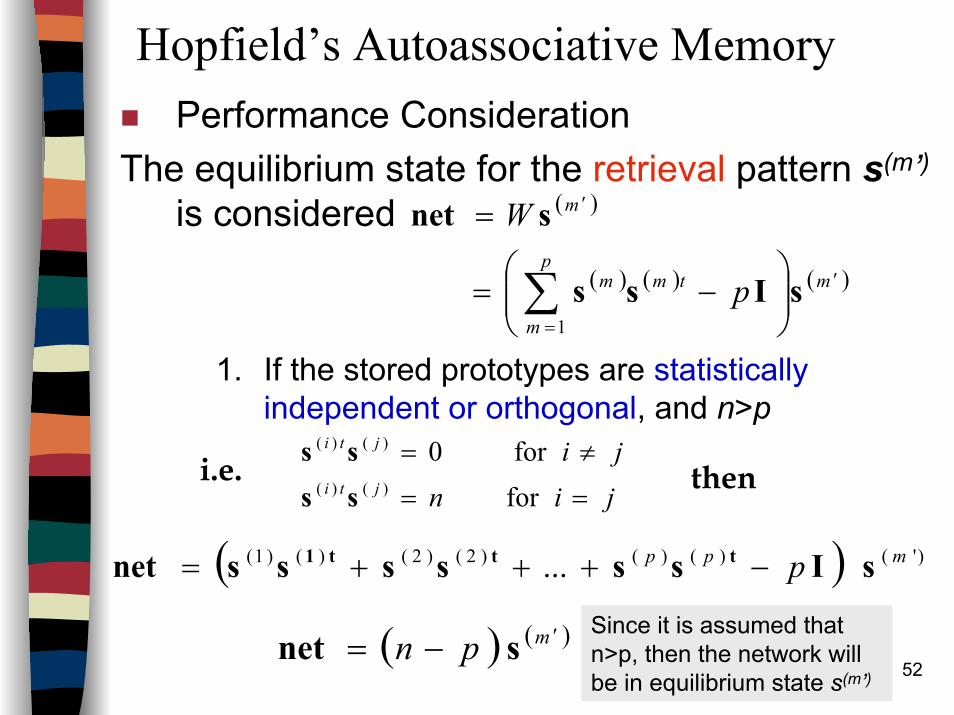
Hopfield’s Autoassociative MemoryPerformance Consideration
The equilibrium state for the retrieval pattern s(m’)is considered
1. If the stored prototypes are statistically independent or orthogonal, and n>p
( )
( ) ( ) ( )mp
m
tmm
m
p
W
′
=
′
−=
=
∑ sIss
snet
1
jinji
jti
jti
==
≠=
for for 0
)()(
)()(
ssss
( ) )'()()()2()2()()1( ... mpp p sIssssssnet ttt1 −+++=
i.e. then
Since it is assumed that n>p, then the network will be in equilibrium state s(m’)
( ) ( )mpn ′−= snet
53
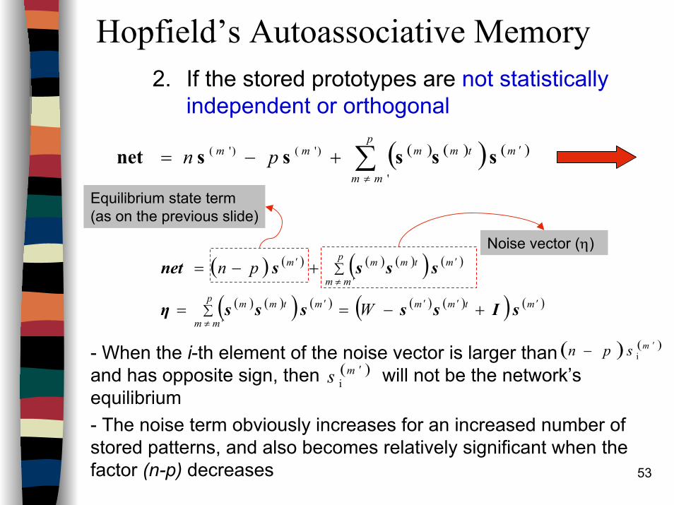
Hopfield’s Autoassociative Memory2. If the stored prototypes are not statistically
independent or orthogonal
( ) ( ) ( ) ( )( ) ( )
( ) ( )( ) ( ) ( ) ( )( ) ( )mtmmmp
mm
tmm
mp
mm
tmmm
W
pn
′′′′
′≠
′
′≠
′
+−==
+−=
∑
∑
sIsssssη
ssssnet
Noise vector (η)
( ) ( )( ) ( )mp
mm
tmmmm pn ′
≠∑+−= sssssnet
'
)'()'(
Equilibrium state term (as on the previous slide)
- When the i-th element of the noise vector is larger than and has opposite sign, then will not be the network’s equilibrium- The noise term obviously increases for an increased number of stored patterns, and also becomes relatively significant when the factor (n-p) decreases
( ) ( )mspn ′− i ( )ms ′i
54
AM and Discrete Hopfield Network.IntroductionBasic ConceptsLinear Associative Memory (Hetero-associative)Hopfield’s AutoassociativeMemoryPerformance Analysis for Recurrent AutoassociationMemoryReferences and suggested reading
IntroductionBasic ConceptsLinear Associative Memory (Hetero-associative)Hopfield’s AutoassociativeMemoryPerformance Analysis for Recurrent AutoassociationMemoryReferences and suggested reading
55
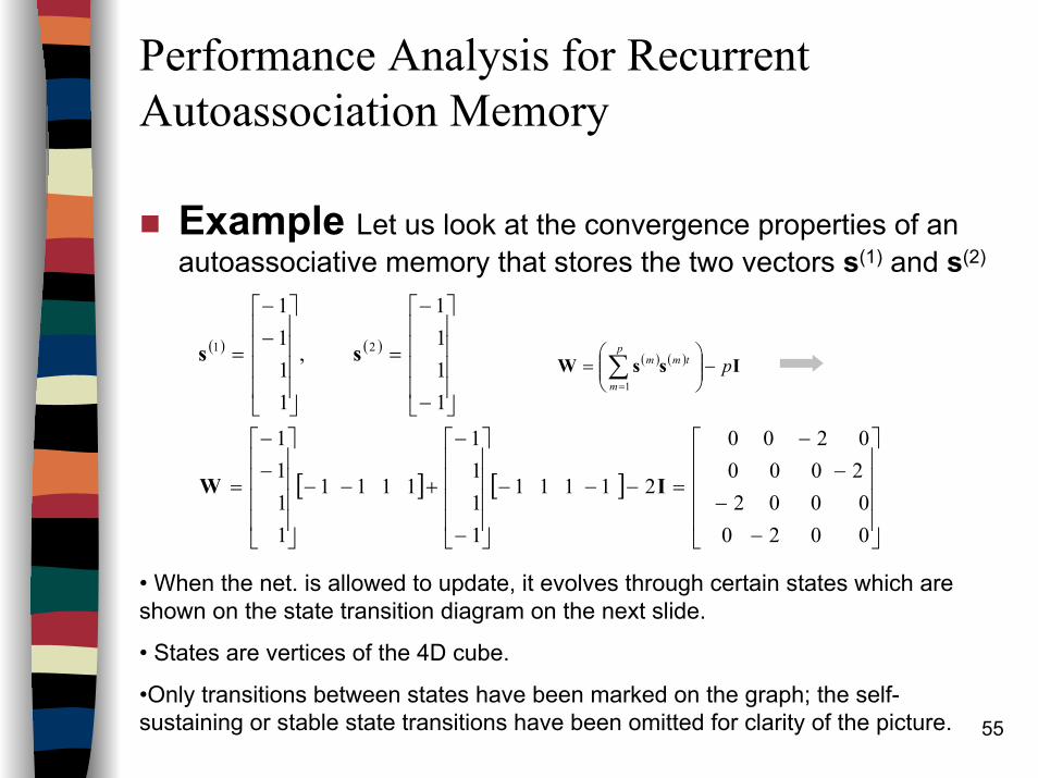
Performance Analysis for Recurrent Autoassociation Memory
Example Let us look at the convergence properties of an autoassociative memory that stores the two vectors s(1) and s(2)
( ) ( )
[ ] [ ]
−−
−−
=−−−
−
−
+−−
−−
=
−
−
=
−−
=
0 0 2 0 0 0 0 2
2 0 0 0 0 2 0 0
2 1 1 1 1
1 1 1 1
1 1 1 1
1 1 11
1 1 1 1
,
1 1 11
21
IW
ss ( ) ( ) IssW pp
m
tmm −
= ∑
=1
• When the net. is allowed to update, it evolves through certain states which are shown on the state transition diagram on the next slide.
• States are vertices of the 4D cube.
•Only transitions between states have been marked on the graph; the self-sustaining or stable state transitions have been omitted for clarity of the picture.
56
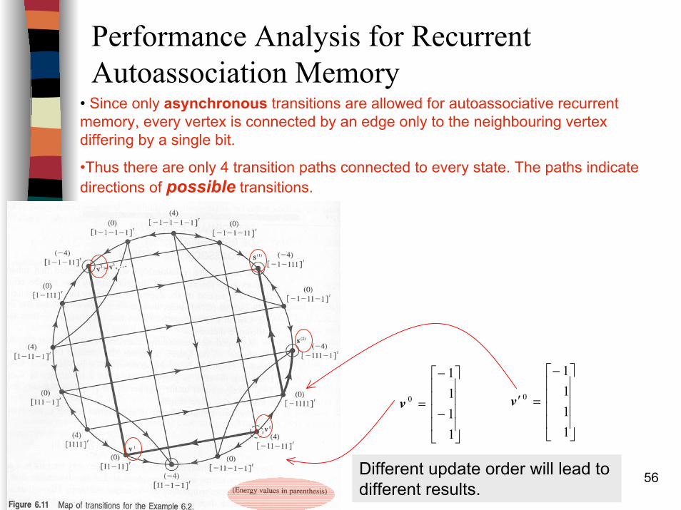
Performance Analysis for Recurrent Autoassociation Memory
• Since only asynchronous transitions are allowed for autoassociative recurrent memory, every vertex is connected by an edge only to the neighbouring vertex differing by a single bit.
•Thus there are only 4 transition paths connected to every state. The paths indicate directions of possible transitions.
−
−
=
1 11 1
0v
−
=′
1 1 1 1
0v
Different update order will lead to different results.
57
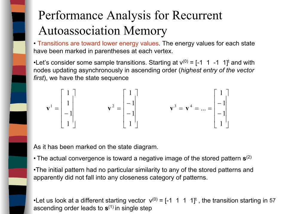
Performance Analysis for Recurrent Autoassociation Memory
• Transitions are toward lower energy values. The energy values for each state have been marked in parentheses at each vertex.
•Let’s consider some sample transitions. Starting at v(0) = [-1 1 -1 1]t and with nodes updating asynchronously in ascending order (highest entry of the vector first), we have the state sequence
As it has been marked on the state diagram.
• The actual convergence is toward a negative image of the stored pattern s(2)
•The initial pattern had no particular similarity to any of the stored patterns and apparently did not fall into any closeness category of patterns.
•Let us look at a different starting vector v(0) = [-1 1 1 1]t , the transition starting in ascending order leads to s(1) in single step
−−
===
−−
=
−=
111
1
...
111
1
11
11
4321 vvvv
58
Performance Analysis for Recurrent Autoassociation Memory
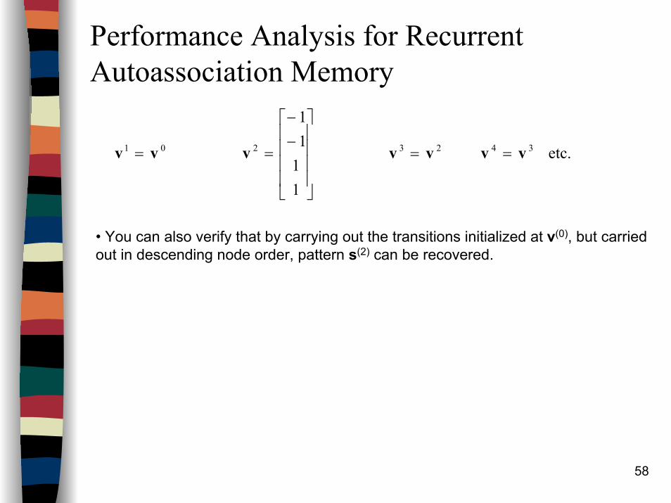
etc.
1111
3423201 vvvvvvv ==
−−
==
• You can also verify that by carrying out the transitions initialized at v(0), but carried out in descending node order, pattern s(2) can be recovered.
59
Advantages and Limits for AssociativeRecurrent Memories
Limits– Limited capability – Converge to spurious memories (states).
Advantage– The recurrences through the thresholding
layer of processing neurons (threshold functions) tend to eliminate noise superimposed on the initializing input vector
60
AM and Discrete Hopfield Network.
IntroductionBasic ConceptsLinear Associative Memory (Hetero-associative)Hopfield’s AutoassociativeMemoryPerformance Analysis for Recurrent AutoassociationMemoryReferences and suggested reading
IntroductionBasic ConceptsLinear Associative Memory (Hetero-associative)Hopfield’s AutoassociativeMemoryPerformance Analysis for Recurrent AutoassociationMemoryReferences and suggested reading
61
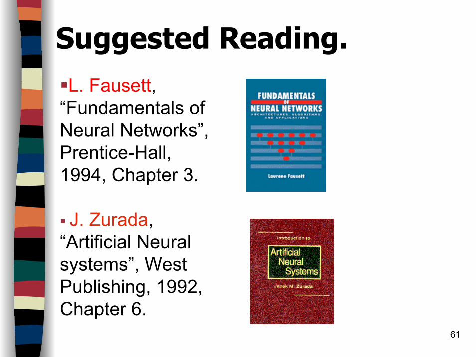
Suggested Reading.L. Fausett,
“Fundamentals of Neural Networks”, Prentice-Hall, 1994, Chapter 3.
J. Zurada, “Artificial Neural systems”, West Publishing, 1992, Chapter 6.
62
References:These lecture notes were based on the references of the
previous slide, and the following references
1. Berlin Chen Lecture notes: Normal University, Taipei, Taiwan, ROC. http://140.122.185.120
2. Dan St. Clair, University of Missori-Rolla, http://web.umr.edu/~stclair/class/classfiles/cs404_fs02/Misc/CS404_fall2001/Lectures/ Lecture 21.