applied artificial neural networks: from associative memories to

5

Applied Artificial Neural Networks: from Associative Memories to

Biomedical Applications

Mahmood Amiri1 and Katayoun Derakhshandeh2, 1Medical Biology Research Centre,

Kermanshah University of Medical Sciences, Kermanshah,

2Department of Pharmaceutics, Faculty of Pharmacy, Kermanshah University of Medical Sciences,

Kermanshah, Iran

1. Introduction

Due to remarkable capabilities of artificial neural networks (ANNs) such as generalization

and nonlinear system modeling, ANNs have been extensively studied and applied in a wide

variety of applications (Amiri et al., 2007; Davande et al., 2008). The rapid development of

ANN technology in recent years has led to an entirely new approach for the solution of

many data processing-based problems, usually encountered in real applications (Hosseini et

al., 2007).

ANNs are characterized in principle by a network topology, a connection pattern, neural

activation properties and a training strategy to process data. In this section, a brief

explanation for four types of ANNs including Multi-Layer Perceptron (MLP), Radial Basis

Function Network (RBFN), Generalized Regression Neural Network (GRNN) and Self-

Feedback Neural Network (SFNN) is provided. The MLP, RBFN and GRNN belong to a

feed-forward class of neural networks (FFNN), while the SFNN belongs to the other

important class of neural networks that is recurrent neural networks (RNN). Next, we

investigate the diverse and innovative applications of these neural networks such as

associative neural networks for recognition of analog and digital patterns, estimating the

release profile of betamethasone (BTM) and betamethasone acetate (BTMA) and

optimization of drug delivery system formulation. Regarding the first application, we

propose a hybrid model consists of the SFNN in parallel with the GRNN. In the proposed

hybrid model, storing of desired patterns is performed by employing a new one-shot

learning algorithm put forward in the chapter. It will be shown that this new hybrid model

is able to perform essential properties found in associative memories such as generalization,

completion and recognition of corrupted patterns. Moreover, a number of case studies are

performed for the purpose of performance comparison between the hybrid model and

others from different classes. For the recurrent associative memory class, the comparison is

www.intechopen.com

Artificial Neural Networks - Methodological Advances and Biomedical Applications

94

made by NDRAM. For comparison with the feed-forward class, the MLP and for the

competitive class, the ART2 are used.

Regarding the second application, ANNs are used in pharmaceutical and pharmacokinetic

areas to model complex interactions and predict the nonlinear relationship between causal

factors and response variables. Specifically, several experiments are performed and an

implant controlled-release system for corticosteroid drug delivery based on biodegradable

polymer is designed. Next, the MLP, GRNN and RBFN are employed to model the release

data and to predict the release profile of BTM and BTMA where in situ forming systems

consist of poly (Lactide-co-glycolide), N-methyl-1-2-pyrolidon and ethyl heptanoat as a

polymer, solvent and additive, respectively. Several simulations are presented to compare

the potential of each neural network. It is demonstrated that the MLP, as a data modeling

tool, is more reliable and efficient than RBFN and GRNN for estimating the release profile of

BTM and BTMA. At the end of this chapter, we investigate the application of the GRNN and

MLP for optimization of drug delivery system formulation. It would appear that GRNN is

promising in providing better solutions for determining drug formulation. Therefore, the

application of the ANNs in biomedical research will definitely increase in the near future.

However, the point which is noteworthy is the fact that there is no single modeling

approach to address all requirements.

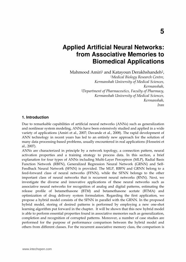
1.1 Multi-Layer Perceptron (MLP) The schematic diagram of an MLP illustrated in Fig.1. In the conventional structure of an

MLP, a neuron receives its input either from other neurons or from external inputs (input

vector). A weighted sum of these inputs constitutes the argument of a nonlinear activation

function. The resulting value of the activation function is the neural output. In this structure,

the weights correspond to the synapses in a biological neuron, while the activation function

is associated with the intracellular current conduction mechanism in the soma. An artificial

neuron is an oversimplified but useful approximation of the biological neuron. This simple

model ignores many of the characteristics of its biological counterpart, e.g. it does not take

into account the time delays that affect the dynamics of the system (Amiri et al., 2009b).

In Fig.1, the output Y of the MLP is a vector with n components determined in the terms of

m components of an input vector X and l components of the hidden layer. The mathematical

representation may be expressed as:

1 1

1,...,l m

i ij jk k wj vij k

y v g w x b b i n= =⎡ ⎤⎛ ⎞= + + =⎢ ⎥⎜ ⎟⎝ ⎠⎣ ⎦∑ ∑ (1)

where vij and wjk are synaptic weights, xk is kth element of the input vector, g(.) is an

activation function and b is the bias which has the effect of increasing or decreasing the net

input of the activation function depending on whether it is positive or negative,

respectively. It has been shown that the MLP with a tanh nonlinearity or other monotonic

nonlinearities is a universal approximator to any arbitrary input-output mappings provided

that some reasonable conditions on the nonlinear mapping are satisfied (Chen and Chen

1995).

www.intechopen.com

Applied Artificial Neural Networks: from Associative Memories to Biomedical Applications

95

Fig. 1. The MLP structure.

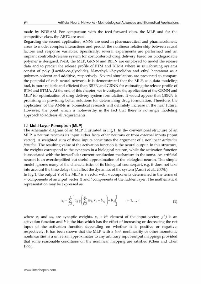
1.2 Radial Basis Function Network (RBFN) Radial basis function neural networks are special classes of the feed-forward neural network models. RBF network is a three-layer network, where each hidden unit implements a radial activation function (a nonlinear transfer function) and each output unit implements a weighted sum of hidden units’ outputs. The structure of the RBF network is shown in Fig. 2. The output of ith neuron in the output layer of the RBF network is determined as follows:

( )1

( ) ; 1,...,M

i ij jj

y x w x c i mϕ=

= − =∑ (2)

where (.)ϕ is the basis function which is described using jx c− , jc is the center vector for hidden neuron j and wij are is the weight between the node j of the hidden layer and the node i of the output layer, m is the number of nodes in the output layer. The norm is typically taken to be the Euclidean distance and the basis function is taken to be Gaussian:

( ) 2

2exp

2

j

jj

x cx cϕ σ

⎧ ⎫−⎪ ⎪− = −⎨ ⎬⎪ ⎪⎩ ⎭ (3)

where jσ is the width parameter of the jth hidden unit in the hidden layer (Amiri et al., 2009). In an RBF network there are three types of parameters that need to be chosen to adapt the

network for a particular task: the center vectors jc , the output weights wij , and the RBF

width parameters jσ . In this way, the training process is usually divided into two steps:

=

www.intechopen.com


96

Fig. 2. The RBFN architecture.

First, the center and width parameters of the hidden layer are determined using only the input data set and by utilizing unsupervised training algorithm such as K-means (Moody and Darken, 1991), decision trees (Kubat, 1998) and self-organizing feature maps (Robert and Hewlett, 2001). Second, the output weights (connecting the hidden layer with the output layer) are determined using both input and output data and by Singular Value Decomposition (SVD) or Least Mean Squared (LMS) algorithms (Bing and Xingshi, 2006). Both steps are relatively fast when compared to back-propagation training algorithm. The number of basis functions controls the complexity and the generalization ability of the RBF network. RBF networks with too few basis functions cannot fit the training data adequately due to limited flexibility.

1.3 Generalize Regression Neural Network (GRNN)

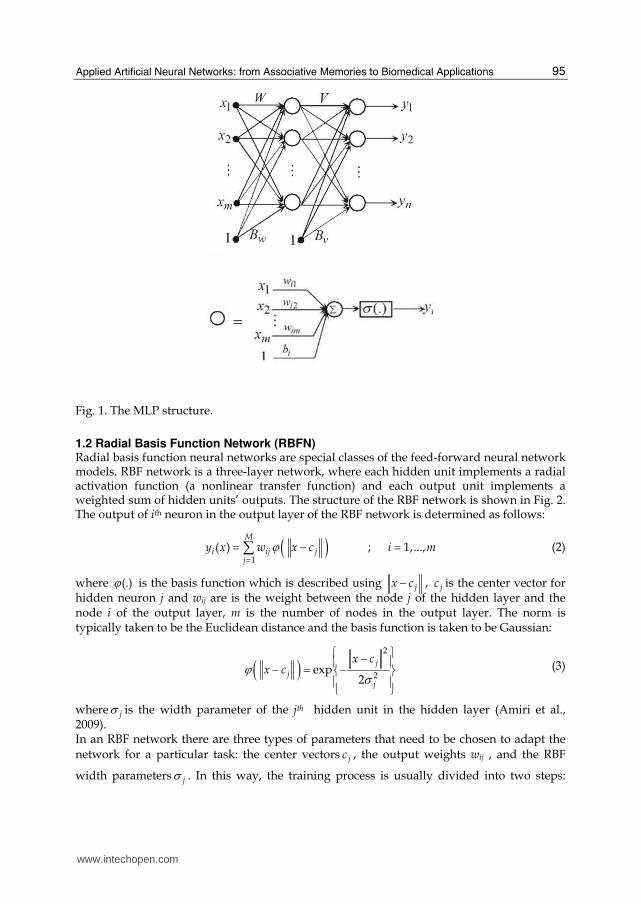
GRNNs belong to the class of neural networks widely used for the continuous function mapping. The main function of a GRNN is to estimate a linear or nonlinear regression surface on independent variables (input vectors) U, given the dependent variables (desired output vectors) X. That is, the network computes the most probable value of an output, x̂ , given only training vectors U. Specifically, the network computes the joint probability density function of U and X. Then the expected value of X given U is expressed as (Wachowiak et al., 2001):

( , )

[ ]

( , )

X f U X dX

E X U

f U X dX

∞−∞∞−∞

= ∫∫

(4)

An important advantage of the GRNN is its simplicity and fast approximation procedure. Another attractive feature is that, unlike back-propagation based neural networks (BP-NN), GRNN does not converge to local minima (Specht, 1991). In addition, the training process with a GRNN-type algorithm is much more efficient than with the BP-NN algorithm (Huang and Williamson, 1994). The topology of a GRNN is described in Fig. 2, and it consists of the following four parts. First, there is an input layer that is fully connected to the pattern layer. Second, there is a pattern layer that has one unit for each pattern. It computes the pattern Gaussian function expressed by

www.intechopen.com


97

2 2 2exp[ 2 ] ; ( ) ( )Ti i i i ih D D u U u Uσ= − = − − (5)

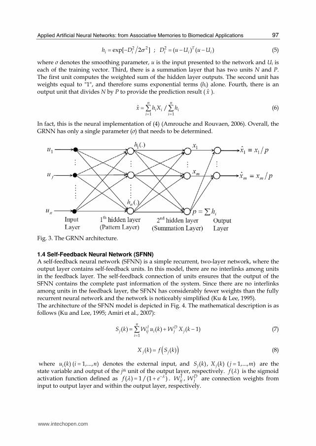
where σ denotes the smoothing parameter, u is the input presented to the network and Ui is each of the training vector. Third, there is a summation layer that has two units N and P. The first unit computes the weighted sum of the hidden layer outputs. The second unit has weights equal to "1", and therefore sums exponential terms (hi) alone. Fourth, there is an output unit that divides N by P to provide the prediction result ( x̂ ).

1 1

ˆ /n n

i i ii i

x h X h= =

= ∑ ∑ (6)

In fact, this is the neural implementation of (4) (Amrouche and Rouvaen, 2006). Overall, the GRNN has only a single parameter (σ) that needs to be determined.

Fig. 3. The GRNN architecture.

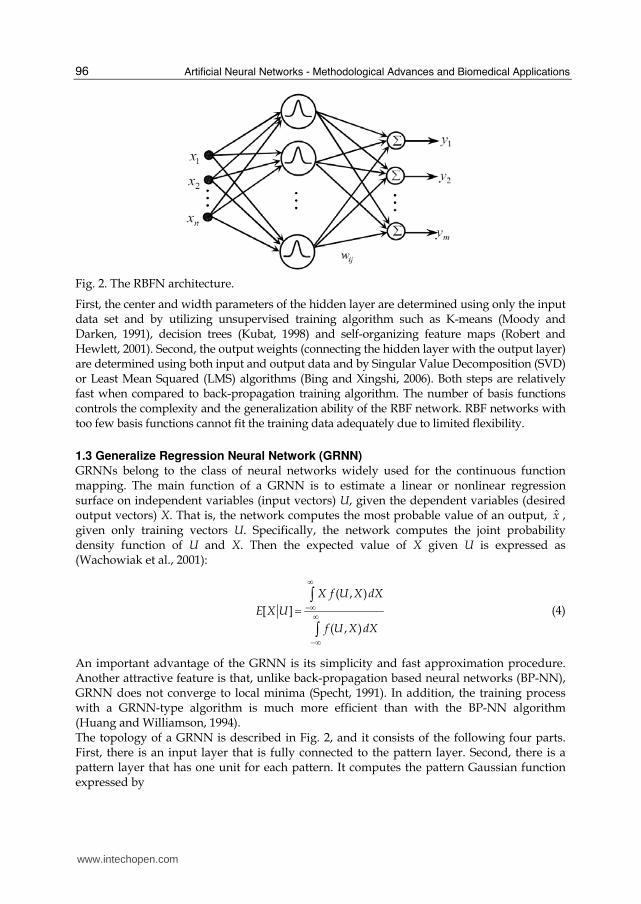
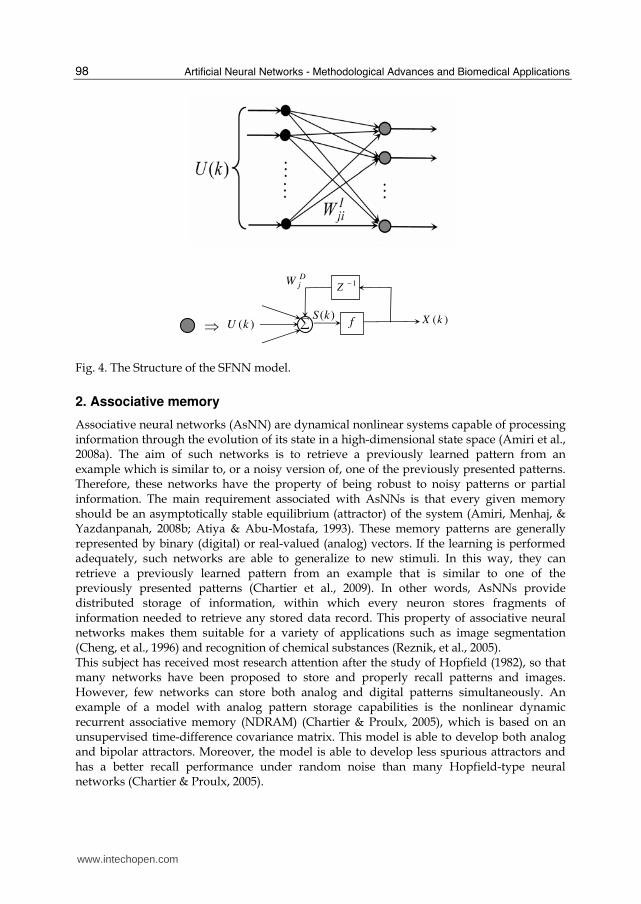
1.4 Self-Feedback Neural Network (SFNN) A self-feedback neural network (SFNN) is a simple recurrent, two-layer network, where the output layer contains self-feedback units. In this model, there are no interlinks among units in the feedback layer. The self-feedback connection of units ensures that the output of the SFNN contains the complete past information of the system. Since there are no interlinks among units in the feedback layer, the SFNN has considerably fewer weights than the fully recurrent neural network and the network is noticeably simplified (Ku & Lee, 1995). The architecture of the SFNN model is depicted in Fig. 4. The mathematical description is as follows (Ku and Lee, 1995; Amiri et al., 2007):

1

( ) ( ) ( 1)n

I Dj ij i j j

i

S k W u k W X k=

= + −∑ (7)

( )( ) ( )j jX k f S k= (8)

where ( ) ( 1,..., )iu k i n= denotes the external input, and ( ) ,jS k ( )jX k ( 1,..., )j m= are the state variable and output of the jth unit of the output layer, respectively. ( )f λ is the sigmoid activation function defined as ( ) 1 /(1 )f e λλ −= + . , I D

ij jW W are connection weights from input to output layer and within the output layer, respectively.

www.intechopen.com


98

Fig. 4. The Structure of the SFNN model.

2. Associative memory

Associative neural networks (AsNN) are dynamical nonlinear systems capable of processing information through the evolution of its state in a high-dimensional state space (Amiri et al., 2008a). The aim of such networks is to retrieve a previously learned pattern from an example which is similar to, or a noisy version of, one of the previously presented patterns. Therefore, these networks have the property of being robust to noisy patterns or partial information. The main requirement associated with AsNNs is that every given memory should be an asymptotically stable equilibrium (attractor) of the system (Amiri, Menhaj, & Yazdanpanah, 2008b; Atiya & Abu-Mostafa, 1993). These memory patterns are generally represented by binary (digital) or real-valued (analog) vectors. If the learning is performed adequately, such networks are able to generalize to new stimuli. In this way, they can retrieve a previously learned pattern from an example that is similar to one of the previously presented patterns (Chartier et al., 2009). In other words, AsNNs provide distributed storage of information, within which every neuron stores fragments of information needed to retrieve any stored data record. This property of associative neural networks makes them suitable for a variety of applications such as image segmentation (Cheng, et al., 1996) and recognition of chemical substances (Reznik, et al., 2005). This subject has received most research attention after the study of Hopfield (1982), so that many networks have been proposed to store and properly recall patterns and images. However, few networks can store both analog and digital patterns simultaneously. An example of a model with analog pattern storage capabilities is the nonlinear dynamic recurrent associative memory (NDRAM) (Chartier & Proulx, 2005), which is based on an unsupervised time-difference covariance matrix. This model is able to develop both analog and bipolar attractors. Moreover, the model is able to develop less spurious attractors and has a better recall performance under random noise than many Hopfield-type neural networks (Chartier & Proulx, 2005).

1Z

−

⇒ f )(kX)(kS)(kU

DjW

∑

www.intechopen.com


99

SFNNs are simple recurrent neural networks that have difficulties learning and storing analog and digital patterns as associative memories (Amiri, et al., 2008b). On the other hand, GRNNs can find a solution for any given problem, but lack a recurrent structure to filter noise. Therefore, in this chapter a hybrid model of SFNN and GRNN for associative recall of analog and digital patterns is proposed.

2.1 The hybrid model

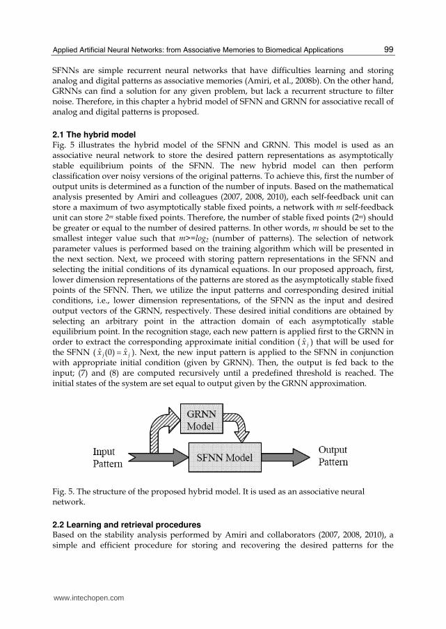
Fig. 5 illustrates the hybrid model of the SFNN and GRNN. This model is used as an associative neural network to store the desired pattern representations as asymptotically stable equilibrium points of the SFNN. The new hybrid model can then perform classification over noisy versions of the original patterns. To achieve this, first the number of output units is determined as a function of the number of inputs. Based on the mathematical analysis presented by Amiri and colleagues (2007, 2008, 2010), each self-feedback unit can store a maximum of two asymptotically stable fixed points, a network with m self-feedback unit can store 2m stable fixed points. Therefore, the number of stable fixed points (2m) should be greater or equal to the number of desired patterns. In other words, m should be set to the smallest integer value such that m>=log2 (number of patterns). The selection of network parameter values is performed based on the training algorithm which will be presented in the next section. Next, we proceed with storing pattern representations in the SFNN and selecting the initial conditions of its dynamical equations. In our proposed approach, first, lower dimension representations of the patterns are stored as the asymptotically stable fixed points of the SFNN. Then, we utilize the input patterns and corresponding desired initial conditions, i.e., lower dimension representations, of the SFNN as the input and desired output vectors of the GRNN, respectively. These desired initial conditions are obtained by selecting an arbitrary point in the attraction domain of each asymptotically stable equilibrium point. In the recognition stage, each new pattern is applied first to the GRNN in order to extract the corresponding approximate initial condition ( ˆ

jx ) that will be used for the SFNN ( ˆ ˆ(0)j jx x= ). Next, the new input pattern is applied to the SFNN in conjunction with appropriate initial condition (given by GRNN). Then, the output is fed back to the input; (7) and (8) are computed recursively until a predefined threshold is reached. The initial states of the system are set equal to output given by the GRNN approximation.

Fig. 5. The structure of the proposed hybrid model. It is used as an associative neural network.

2.2 Learning and retrieval procedures Based on the stability analysis performed by Amiri and collaborators (2007, 2008, 2010), a simple and efficient procedure for storing and recovering the desired patterns for the

www.intechopen.com


100

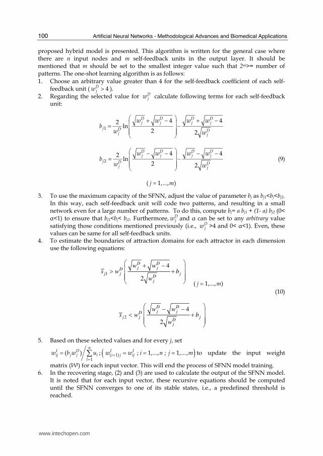
proposed hybrid model is presented. This algorithm is written for the general case where there are n input nodes and m self-feedback units in the output layer. It should be mentioned that m should be set to the smallest integer value such that 2m>= number of patterns. The one-shot learning algorithm is as follows:

1. Choose an arbitrary value greater than 4 for the self-feedback coefficient of each self-feedback unit ( 4D

jw > ). 2. Regarding the selected value for D

jw calculate following terms for each self-feedback unit:

1

4 42ln

2 2

D D D Dj j j j

j D Dj j

w w w wb

w w

⎛ ⎞+ − + −⎜ ⎟= −⎜ ⎟⎜ ⎟⎝ ⎠

2

4 42ln

2 2

D D D Dj j j j

j D Dj j

w w w wb

w w

⎛ ⎞− − − −⎜ ⎟= −⎜ ⎟⎜ ⎟⎝ ⎠ (9)

( 1,..., )j m=

3. To use the maximum capacity of the SFNN, adjust the value of parameter bj as bj1<bj<bj2. In this way, each self-feedback unit will code two patterns, and resulting in a small network even for a large number of patterns. To do this, compute bj= α bj1 + (1- α) bj2 (0< α<1) to ensure that bj1<bj< bj2. Furthermore, D

jw and α can be set to any arbitrary value satisfying those conditions mentioned previously (i.e., D

jw >4 and 0< α<1). Even, these values can be same for all self-feedback units.

4. To estimate the boundaries of attraction domains for each attractor in each dimension use the following equations:

1

4

2

D Dj jD

j j jDj

w ws w b

w

⎛ ⎞+ −⎜ ⎟> +⎜ ⎟⎜ ⎟⎝ ⎠ ( 1,..., )j m=

(10)

2

4

2

D Dj jD

j j jDj

w ws w b

w

⎛ ⎞− −⎜ ⎟< +⎜ ⎟⎜ ⎟⎝ ⎠

5. Based on these selected values and for every j, set

( )( 1)1

( ) ; ; 1,..., ; 1,... ,n

I D I Iij j j l i j ij

l

w b w u w w i n j m+== = = =∑ to update the input weight

matrix (WI) for each input vector. This will end the process of SFNN model training. 6. In the recovering stage, (2) and (3) are used to calculate the output of the SFNN model.

It is noted that for each input vector, these recursive equations should be computed until the SFNN converges to one of its stable states, i.e., a predefined threshold is reached.

www.intechopen.com


101

3. Simulation results

In this section, simulations on auto-associative tasks are presented in order to assess the efficiency of the hybrid model. We have studied two tasks. The first task consists of learning and retrieving a numeral data set (bipolar representation) while the second task consists of learning a pictorial data set (analog representation). Gaussian basis functions with constant smoothing parameters (σ=0.85) were used for the GRNN throughout this study. All experiments were implemented in MATLAB (ver.7) on a personal computer with AMD Athlon 64 bit Processor 3500+.

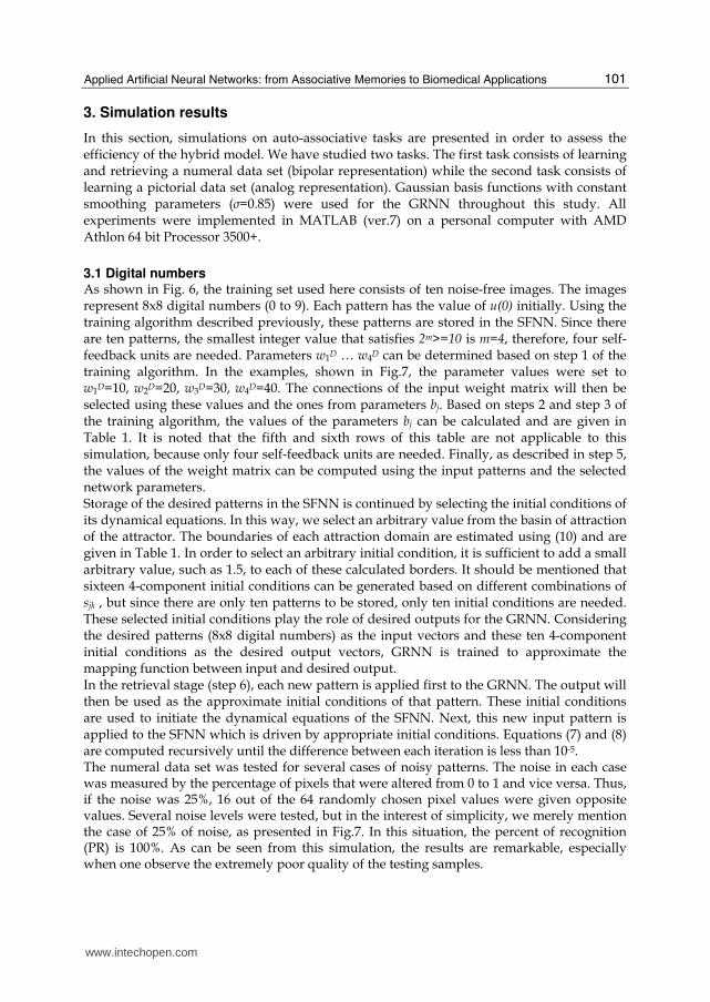
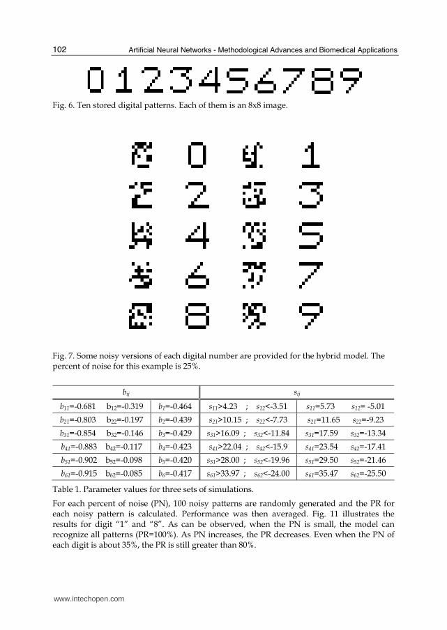
3.1 Digital numbers As shown in Fig. 6, the training set used here consists of ten noise-free images. The images represent 8x8 digital numbers (0 to 9). Each pattern has the value of u(0) initially. Using the training algorithm described previously, these patterns are stored in the SFNN. Since there are ten patterns, the smallest integer value that satisfies 2m>=10 is m=4, therefore, four self-feedback units are needed. Parameters w1D … w4D can be determined based on step 1 of the training algorithm. In the examples, shown in Fig.7, the parameter values were set to w1D=10, w2D=20, w3D=30, w4D=40. The connections of the input weight matrix will then be selected using these values and the ones from parameters bj. Based on steps 2 and step 3 of the training algorithm, the values of the parameters bj can be calculated and are given in Table 1. It is noted that the fifth and sixth rows of this table are not applicable to this simulation, because only four self-feedback units are needed. Finally, as described in step 5, the values of the weight matrix can be computed using the input patterns and the selected network parameters. Storage of the desired patterns in the SFNN is continued by selecting the initial conditions of its dynamical equations. In this way, we select an arbitrary value from the basin of attraction of the attractor. The boundaries of each attraction domain are estimated using (10) and are given in Table 1. In order to select an arbitrary initial condition, it is sufficient to add a small arbitrary value, such as 1.5, to each of these calculated borders. It should be mentioned that sixteen 4-component initial conditions can be generated based on different combinations of sjk , but since there are only ten patterns to be stored, only ten initial conditions are needed. These selected initial conditions play the role of desired outputs for the GRNN. Considering the desired patterns (8x8 digital numbers) as the input vectors and these ten 4-component initial conditions as the desired output vectors, GRNN is trained to approximate the mapping function between input and desired output. In the retrieval stage (step 6), each new pattern is applied first to the GRNN. The output will then be used as the approximate initial conditions of that pattern. These initial conditions are used to initiate the dynamical equations of the SFNN. Next, this new input pattern is applied to the SFNN which is driven by appropriate initial conditions. Equations (7) and (8) are computed recursively until the difference between each iteration is less than 10-5. The numeral data set was tested for several cases of noisy patterns. The noise in each case was measured by the percentage of pixels that were altered from 0 to 1 and vice versa. Thus, if the noise was 25%, 16 out of the 64 randomly chosen pixel values were given opposite values. Several noise levels were tested, but in the interest of simplicity, we merely mention the case of 25% of noise, as presented in Fig.7. In this situation, the percent of recognition (PR) is 100%. As can be seen from this simulation, the results are remarkable, especially when one observe the extremely poor quality of the testing samples.

www.intechopen.com


102

Fig. 6. Ten stored digital patterns. Each of them is an 8x8 image.

Fig. 7. Some noisy versions of each digital number are provided for the hybrid model. The percent of noise for this example is 25%.

bij sij

b11=-0.681 b12=-0.319 b1=-0.464 s11>4.23 ; s12<-3.51 s11=5.73 s12= -5.01

b21=-0.803 b22=-0.197 b2=-0.439 s21>10.15 ; s22<-7.73 s21=11.65 s22=-9.23

b31=-0.854 b32=-0.146 b3=-0.429 s31>16.09 ; s32<-11.84 s31=17.59 s32=-13.34

b41=-0.883 b42=-0.117 b4=-0.423 s41>22.04 ; s42<-15.9 s41=23.54 s42=-17.41

b51=-0.902 b52=-0.098 b5=-0.420 s51>28.00 ; s52<-19.96 s51=29.50 s52=-21.46

b61=-0.915 b62=-0.085 b6=-0.417 s61>33.97 ; s62<-24.00 s61=35.47 s62=-25.50

Table 1. Parameter values for three sets of simulations.

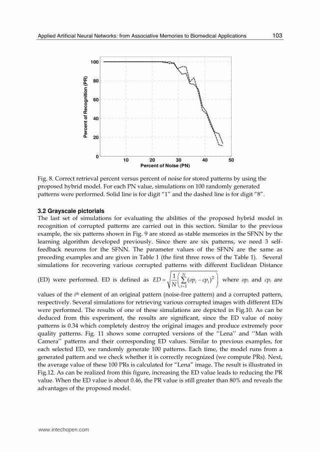
For each percent of noise (PN), 100 noisy patterns are randomly generated and the PR for each noisy pattern is calculated. Performance was then averaged. Fig. 11 illustrates the results for digit “1” and “8”. As can be observed, when the PN is small, the model can recognize all patterns (PR=100%). As PN increases, the PR decreases. Even when the PN of each digit is about 35%, the PR is still greater than 80%.

www.intechopen.com


103

10 20 30 40 500

20

40

60

80

100

Percent of Noise (PN)

Perc

en

t o

f R

eco

gn

itio

n (P

R)

Fig. 8. Correct retrieval percent versus percent of noise for stored patterns by using the

proposed hybrid model. For each PN value, simulations on 100 randomly generated

patterns were performed. Solid line is for digit “1” and the dashed line is for digit “8”.

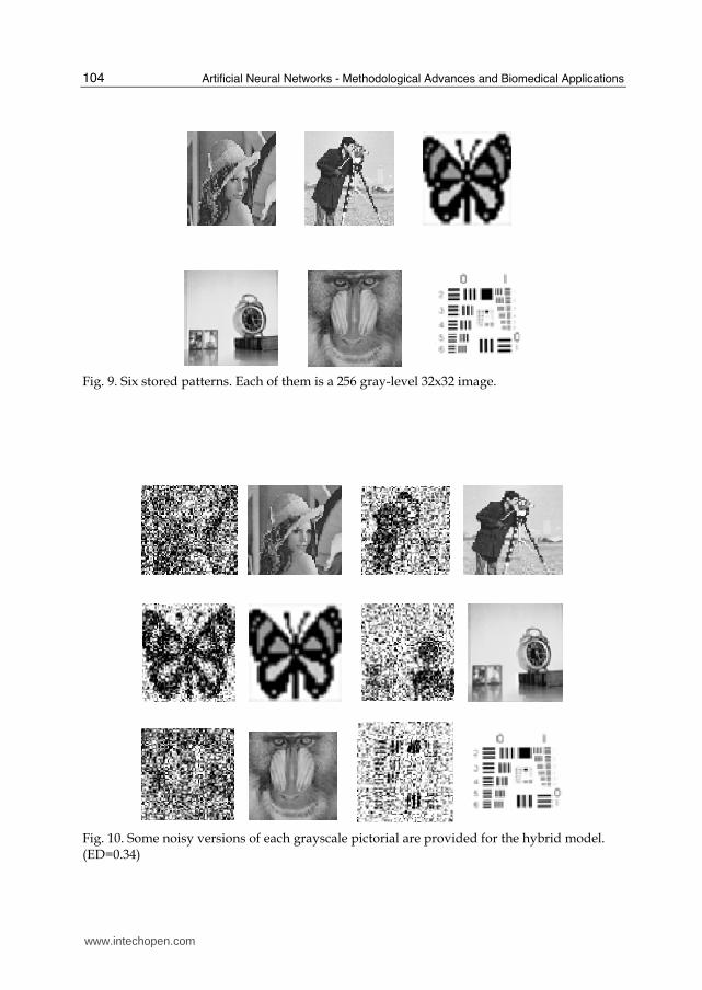
3.2 Grayscale pictorials The last set of simulations for evaluating the abilities of the proposed hybrid model in

recognition of corrupted patterns are carried out in this section. Similar to the previous

example, the six patterns shown in Fig. 9 are stored as stable memories in the SFNN by the

learning algorithm developed previously. Since there are six patterns, we need 3 self-

feedback neurons for the SFNN. The parameter values of the SFNN are the same as

preceding examples and are given in Table 1 (the first three rows of the Table 1). Several

simulations for recovering various corrupted patterns with different Euclidean Distance

(ED) were performed. ED is defined as 2

1

1( )

N

i ii

ED op cpN =⎛ ⎞= −⎜ ⎟⎝ ⎠∑ where opi and cpi are

values of the ith element of an original pattern (noise-free pattern) and a corrupted pattern,

respectively. Several simulations for retrieving various corrupted images with different EDs

were performed. The results of one of these simulations are depicted in Fig.10. As can be

deduced from this experiment, the results are significant, since the ED value of noisy

patterns is 0.34 which completely destroy the original images and produce extremely poor

quality patterns. Fig. 11 shows some corrupted versions of the ‘‘Lena’’ and ‘‘Man with

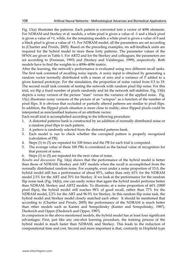
Camera’’ patterns and their corresponding ED values. Similar to previous examples, for

each selected ED, we randomly generate 100 patterns. Each time, the model runs from a

generated pattern and we check whether it is correctly recognized (we compute PRs). Next,

the average value of these 100 PRs is calculated for “Lena” image. The result is illustrated in

Fig.12. As can be realized from this figure, increasing the ED value leads to reducing the PR

value. When the ED value is about 0.46, the PR value is still greater than 80% and reveals the

advantages of the proposed model.

www.intechopen.com


104

Fig. 9. Six stored patterns. Each of them is a 256 gray-level 32x32 image.

Fig. 10. Some noisy versions of each grayscale pictorial are provided for the hybrid model. (ED=0.34)

www.intechopen.com


105

ED= 0.289 ED= 0.331 ED= 0.423

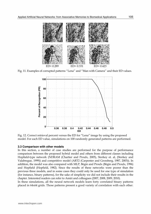
Fig. 11. Examples of corrupted patterns ‘‘Lena’’ and ‘‘Man with Camera’’ and their ED values.

0.36 0.38 0.4 0.42 0.44 0.46 0.48 0.5 0

20

40

60

80

100

ED

Perc

en

t o

f R

eco

gn

itio

n (P

R)

Fig. 12. Correct retrieval percent versus the ED for “Lena” image by using the proposed model. For each ED value, simulations on 100 randomly generated patterns are performed.

3.3 Comparison with other models In this section, a number of case studies are performed for the purpose of performance comparison between the proposed hybrid model and others from different classes including Hopfield-type network (NDRAM (Chartier and Proulx, 2005), Storkey et. al, (Storkey and Valabregue, 1999)) and competitive model (ART2 (Carpenter and Grossberg, 1987, 2003)). In addition, the model was also compared with MLP, Bégin and Proulx (Bégin and Proulx, 1996) and Hopfield (Hopfield, 1982). Since the results of these networks were poorer than the previous three models, and in some cases they could only be used for one type of simulation (for instance, binary patterns), for the sake of simplicity we did not include their results in the chapter. Interested readers can refer to Amiri and colleagues (2007, 2008, 2009, 2010). In these simulations, all the neural network models learn forty correlated binary patterns placed in 64x64 grids. Those patterns present a good variety of correlation with each other.

www.intechopen.com


106

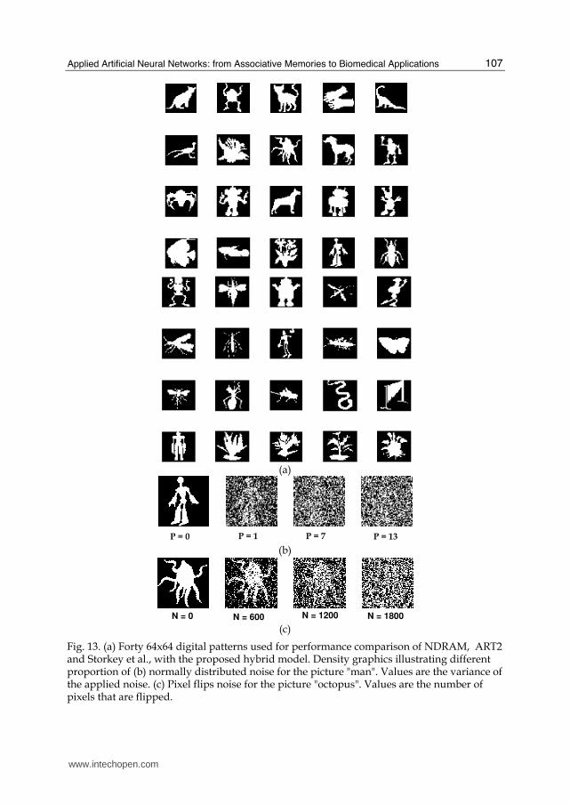
Fig. 13(a) illustrates the patterns. Each pattern is converted into a vector of 4096 elements. For NDRAM and Storkey et al. models, a white pixel is given a value of -1 and a black pixel is given a value of +1, while, for the remaining models a white pixel is given a value of 0 and a black pixel is given a value of +1. For NDRAM model, all the parameters are set according to (Chartier and Proulx, 2005). Based on the preceding examples, six self-feedback units are required for the hybrid model to store these forty patterns. The parameter values of the SFNN are given in Table 1. For ART2 and for the Storkey and colleagues, the parameters are set according to (Freeman, 1993) and (Storkey and Valabregue, 1999), respectively. Both

models have to find the weights in a 4096×4096 matrix. After the learning, the network’s performance is evaluated using two different recall tasks. The first task consisted of recalling noisy inputs. A noisy input is obtained by generating a random vector normally distributed with a mean of zero and a variance of P added to a given learned prototype. For the simulation, the proportion of noise varied from 0.5 to 19. The second recall task consists of testing the network with random pixel flip noise. For this trial, we flip a fixed number of pixels randomly and let the network self-stabilize. Fig. 13(b) depicts a noisy version of the picture “man” versus the variance of the applied noise. Fig. 13(c) illustrates noisy versions of the picture of an “octopus” as a function of the number of pixel flips. It is obvious that occluded or partially altered patterns are similar to pixel flips. In addition, the flipped pixels situation is more close to reality; since flipped pixels could be interpreted as misclassified features of an attribute vector. Each recall trial is accomplished according to the following procedure: 1. A distorted patterns bank is constructed by an addition of normally distributed noise or

a random pixel flips to each pattern. 2. A pattern is randomly selected from the distorted patterns bank. 3. Each model is run to check whether the corrupted pattern is properly recognized

(calculation of PR). 4. Steps (1) to (3) are repeated for 100 times and the PR for each trial is computed. 5. The average value of these 100 PRs is considered as the factual value of recognition for

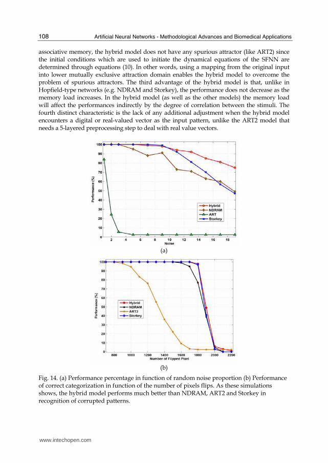
that percent of noise. 6. Steps (1) to (5) are repeated for the next value of noise. Results and discussion: Fig. 14(a) shows that the performance of the hybrid model is better than those of NDRAM, Storkey and ART models when the recall is accomplished from the normally distributed random noise. For example, even under a noise proportion of 15.0, the hybrid model still has a performance of about 85%, rather than only 63% for the NDRAM model 2.5% for the ART and 70% for Storkey. If we look at the performance for the random flip noise task (Fig. 14(b)), one can easily notice that again the hybrid model performs better than NDRAM, Storkey and ART2 models. To illustrate, at a noise proportion of 44% (1800 pixel flips), the hybrid model still reaches 98% of good recall, rather than 77% for the NDRAM model, 2.5% for the ART and 96.9% for Storkey. In this random flip noise task, the hybrid model and Storkey model closely matched each other. It should be mentioned that according to (Chartier and Proulx, 2005) the performance of the NDRAM is much better than other models such as Kanter and Sompolinsky (Kanter and Sompolinsky, 1987), Diederich and Opper (Diederich and Opper, 1987). In comparison to the above-mentioned models, the hybrid model has at least four significant advantages: First, just like any one-shot learning procedure, the training process of the hybrid model is much faster than NDRAM, and Storkey. This leads to the reduction of computational time and cost. Second and more important is that, contrarily to Hopfield-type

www.intechopen.com


107

(a)

(b)

(c)

Fig. 13. (a) Forty 64x64 digital patterns used for performance comparison of NDRAM, ART2 and Storkey et al., with the proposed hybrid model. Density graphics illustrating different proportion of (b) normally distributed noise for the picture "man". Values are the variance of the applied noise. (c) Pixel flips noise for the picture "octopus". Values are the number of pixels that are flipped.

N = 0 N = 1800N = 600 N = 1200

P = 0 P = 1 P = 13P = 7

www.intechopen.com


108

associative memory, the hybrid model does not have any spurious attractor (like ART2) since the initial conditions which are used to initiate the dynamical equations of the SFNN are determined through equations (10). In other words, using a mapping from the original input into lower mutually exclusive attraction domain enables the hybrid model to overcome the problem of spurious attractors. The third advantage of the hybrid model is that, unlike in Hopfield-type networks (e.g. NDRAM and Storkey), the performance does not decrease as the memory load increases. In the hybrid model (as well as the other models) the memory load will affect the performances indirectly by the degree of correlation between the stimuli. The fourth distinct characteristic is the lack of any additional adjustment when the hybrid model encounters a digital or real-valued vector as the input pattern, unlike the ART2 model that needs a 5-layered preprocessing step to deal with real value vectors.

(a)

(b)

Fig. 14. (a) Performance percentage in function of random noise proportion (b) Performance of correct categorization in function of the number of pixels flips. As these simulations shows, the hybrid model performs much better than NDRAM, ART2 and Storkey in recognition of corrupted patterns.

www.intechopen.com


109

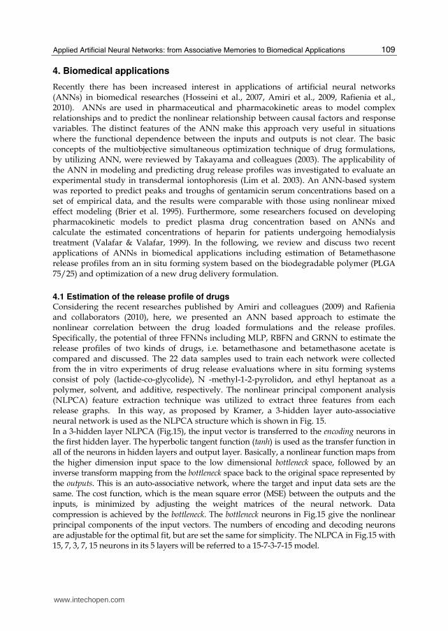
4. Biomedical applications

Recently there has been increased interest in applications of artificial neural networks (ANNs) in biomedical researches (Hosseini et al., 2007, Amiri et al., 2009, Rafienia et al., 2010). ANNs are used in pharmaceutical and pharmacokinetic areas to model complex relationships and to predict the nonlinear relationship between causal factors and response variables. The distinct features of the ANN make this approach very useful in situations where the functional dependence between the inputs and outputs is not clear. The basic concepts of the multiobjective simultaneous optimization technique of drug formulations, by utilizing ANN, were reviewed by Takayama and colleagues (2003). The applicability of the ANN in modeling and predicting drug release profiles was investigated to evaluate an experimental study in transdermal iontophoresis (Lim et al. 2003). An ANN-based system was reported to predict peaks and troughs of gentamicin serum concentrations based on a set of empirical data, and the results were comparable with those using nonlinear mixed effect modeling (Brier et al. 1995). Furthermore, some researchers focused on developing pharmacokinetic models to predict plasma drug concentration based on ANNs and calculate the estimated concentrations of heparin for patients undergoing hemodialysis treatment (Valafar & Valafar, 1999). In the following, we review and discuss two recent applications of ANNs in biomedical applications including estimation of Betamethasone release profiles from an in situ forming system based on the biodegradable polymer (PLGA 75/25) and optimization of a new drug delivery formulation.

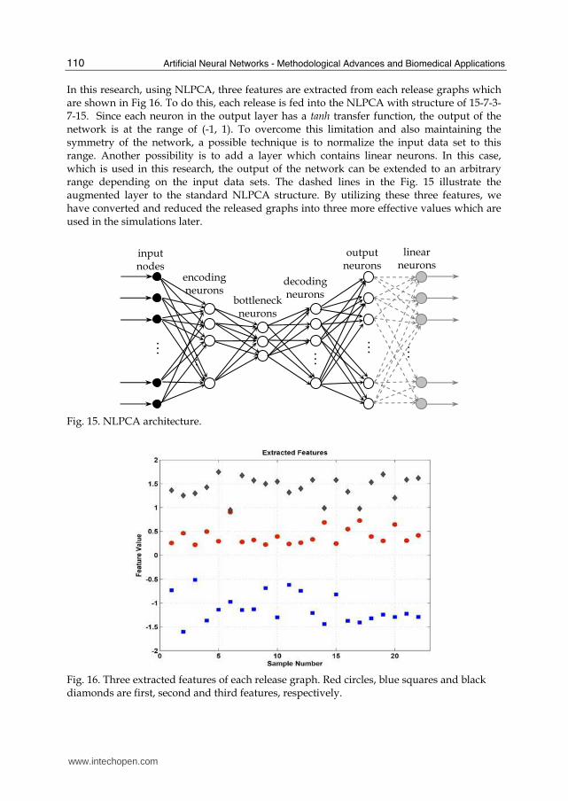
4.1 Estimation of the release profile of drugs Considering the recent researches published by Amiri and colleagues (2009) and Rafienia and collaborators (2010), here, we presented an ANN based approach to estimate the nonlinear correlation between the drug loaded formulations and the release profiles. Specifically, the potential of three FFNNs including MLP, RBFN and GRNN to estimate the release profiles of two kinds of drugs, i.e. betamethasone and betamethasone acetate is compared and discussed. The 22 data samples used to train each network were collected from the in vitro experiments of drug release evaluations where in situ forming systems consist of poly (lactide-co-glycolide), N -methyl-1-2-pyrolidon, and ethyl heptanoat as a polymer, solvent, and additive, respectively. The nonlinear principal component analysis (NLPCA) feature extraction technique was utilized to extract three features from each release graphs. In this way, as proposed by Kramer, a 3-hidden layer auto-associative neural network is used as the NLPCA structure which is shown in Fig. 15. In a 3-hidden layer NLPCA (Fig.15), the input vector is transferred to the encoding neurons in the first hidden layer. The hyperbolic tangent function (tanh) is used as the transfer function in all of the neurons in hidden layers and output layer. Basically, a nonlinear function maps from the higher dimension input space to the low dimensional bottleneck space, followed by an inverse transform mapping from the bottleneck space back to the original space represented by the outputs. This is an auto-associative network, where the target and input data sets are the same. The cost function, which is the mean square error (MSE) between the outputs and the inputs, is minimized by adjusting the weight matrices of the neural network. Data compression is achieved by the bottleneck. The bottleneck neurons in Fig.15 give the nonlinear principal components of the input vectors. The numbers of encoding and decoding neurons are adjustable for the optimal fit, but are set the same for simplicity. The NLPCA in Fig.15 with 15, 7, 3, 7, 15 neurons in its 5 layers will be referred to a 15-7-3-7-15 model.

www.intechopen.com


110

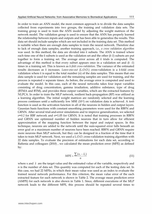
In this research, using NLPCA, three features are extracted from each release graphs which are shown in Fig 16. To do this, each release is fed into the NLPCA with structure of 15-7-3-7-15. Since each neuron in the output layer has a tanh transfer function, the output of the network is at the range of (-1, 1). To overcome this limitation and also maintaining the symmetry of the network, a possible technique is to normalize the input data set to this range. Another possibility is to add a layer which contains linear neurons. In this case, which is used in this research, the output of the network can be extended to an arbitrary range depending on the input data sets. The dashed lines in the Fig. 15 illustrate the augmented layer to the standard NLPCA structure. By utilizing these three features, we have converted and reduced the released graphs into three more effective values which are used in the simulations later.

Fig. 15. NLPCA architecture.

Fig. 16. Three extracted features of each release graph. Red circles, blue squares and black diamonds are first, second and third features, respectively.

BB

B B B

encoding neurons

bottleneck neurons

decoding neurons

output neurons

linear neurons

input nodes

www.intechopen.com


111

In order to train an ANN model, the most common approach is to divide the data samples collected from experiments into two groups, the training and validation data sets. The training group is used to train the ANN model by adjusting the weight matrices of the network model. The validation group is used to ensure that the ANN has properly learned the relationship between inputs and outputs and has been able to generalize the results. This data set should include samples which are not included in the training data set. This method is suitable when there are enough data samples to train the neural network. Therefore due to lack of enough data samples, another training approach, i.e., a cross validation algorithm was used. In this method, the data are divided into k subsets. The ANN is trained where each time one of the k subsets is used as the validation set and the other (k-1) subsets are put together to form a training set. The average error across all k trials is computed. The advantage of this method is that every subset appears once in a validation set and (k -1) times in a training set. This is known as k-fold cross-validation. The variance of the estimated results decreases as k increases. Leave-one-out (L.O.O.) cross-validation is a k-fold cross validation where k is equal to the total number (n) of the data samples. This means that one data sample is used for validation and the remaining samples are used for training, and the process is repeated n separate times. As before, the average error is computed and used to evaluate the model. In this case, each of the neural networks takes four input variables consisting of drug concentration, gamma irradiation, additive substance, type of drug (BTMA and BTM), and provides three output variables, which are the extracted features by NLPCA. In order to train the MLP network, resilient back-propagation (RP) was utilized as a learning algorithm. The initial weight matrices are randomly selected and the learning process continues until a sufficiently low MSE (10-3) on validation data is achieved. A tanh function is used as the activation function in all of the neurons in hidden and output layers. Gaussian basis functions with constant smoothing parameters were used for the RBFN and GRNN. After several trial-and-error simulations and to improve generalization, we selected σ=0.2 for RBF network and σ=1.05 for GRNN. It is noted that training processes in RBFN and GRNN use optimized number of hidden neurons that in turn allow for efficient approximation of the mapping function between the input and output spaces. In this technique, neurons are added to the network until the sum-squared error falls beneath an error goal or a maximum number of neurons have been reached. RBFN and GRNN require more neurons than MLP network, but they can be designed in a fraction of the time that it takes to train MLP network. Next, we used a L.O.O. cross-validation training algorithm with 22 data samples. To evaluate the precision of estimations for each data set, according to Rafienia and colleagues (2010) , we calculated the mean prediction error (MPE) as defined by:

ˆ( )i ix x

MPEn

−= ∑ (11)

where x and x̂ are the target value and the estimated value of the variable, respectively and

n is the number of data set. This quantity was computed for each of the testing data set. In this case, we had 22 MPEs, in which their mean value was used as an index to evaluate the trained neural network performance. For this criterion, the mean value error of the each extracted feature for each network is shown in Table 2. The average mean prediction error (AMPE) for each network is also shown in Table 1. Since, different executions of the MLP network leads to the different MPE, this process should be repeated several times to

www.intechopen.com


112

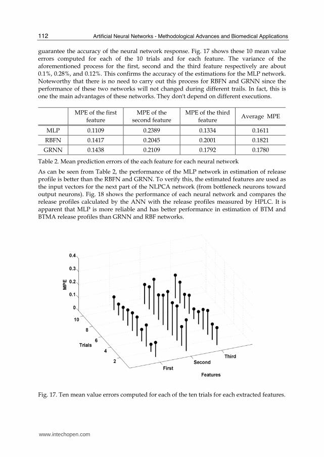
guarantee the accuracy of the neural network response. Fig. 17 shows these 10 mean value errors computed for each of the 10 trials and for each feature. The variance of the aforementioned process for the first, second and the third feature respectively are about 0.1%, 0.28%, and 0.12%. This confirms the accuracy of the estimations for the MLP network. Noteworthy that there is no need to carry out this process for RBFN and GRNN since the performance of these two networks will not changed during different trails. In fact, this is one the main advantages of these networks. They don't depend on different executions.

MPE of the first

feature MPE of the

second feature MPE of the third

feature Average MPE

MLP 0.1109 0.2389 0.1334 0.1611

RBFN 0.1417 0.2045 0.2001 0.1821

GRNN 0.1438 0.2109 0.1792 0.1780

Table 2. Mean prediction errors of the each feature for each neural network

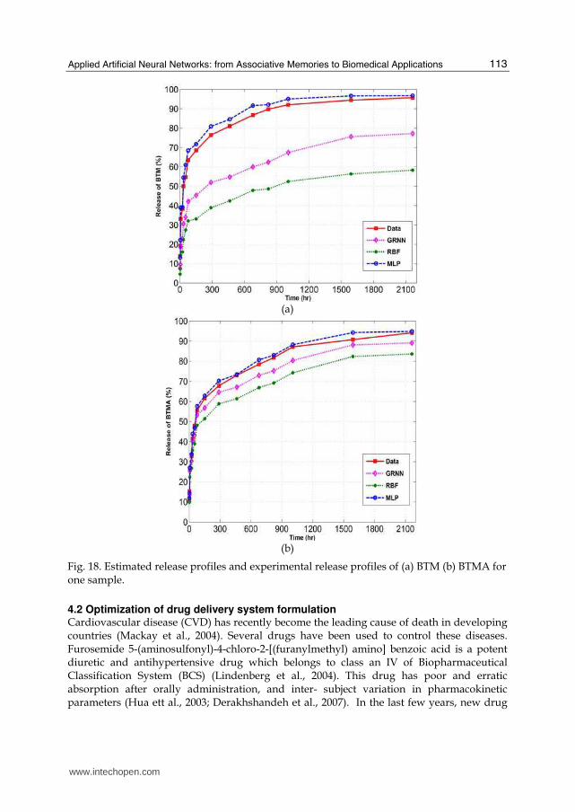
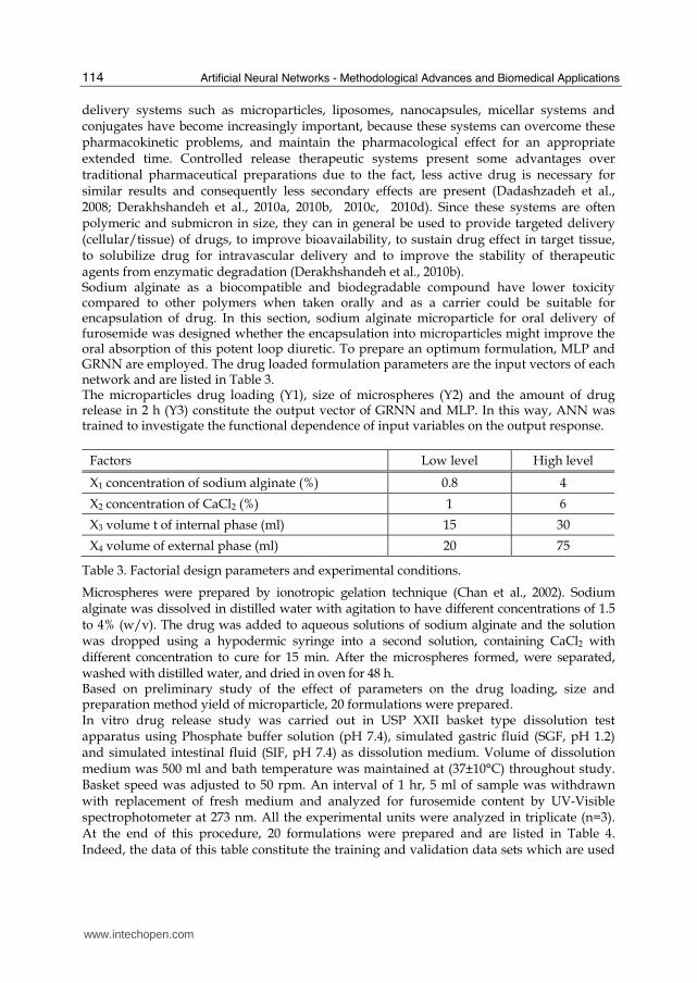
As can be seen from Table 2, the performance of the MLP network in estimation of release profile is better than the RBFN and GRNN. To verify this, the estimated features are used as the input vectors for the next part of the NLPCA network (from bottleneck neurons toward output neurons). Fig. 18 shows the performance of each neural network and compares the release profiles calculated by the ANN with the release profiles measured by HPLC. It is apparent that MLP is more reliable and has better performance in estimation of BTM and BTMA release profiles than GRNN and RBF networks.

Fig. 17. Ten mean value errors computed for each of the ten trials for each extracted features.

www.intechopen.com


113

(a)

(b)

Fig. 18. Estimated release profiles and experimental release profiles of (a) BTM (b) BTMA for one sample.

4.2 Optimization of drug delivery system formulation Cardiovascular disease (CVD) has recently become the leading cause of death in developing countries (Mackay et al., 2004). Several drugs have been used to control these diseases. Furosemide 5-(aminosulfonyl)-4-chloro-2-[(furanylmethyl) amino] benzoic acid is a potent diuretic and antihypertensive drug which belongs to class an IV of Biopharmaceutical Classification System (BCS) (Lindenberg et al., 2004). This drug has poor and erratic absorption after orally administration, and inter- subject variation in pharmacokinetic parameters (Hua ett al., 2003; Derakhshandeh et al., 2007). In the last few years, new drug

www.intechopen.com


114

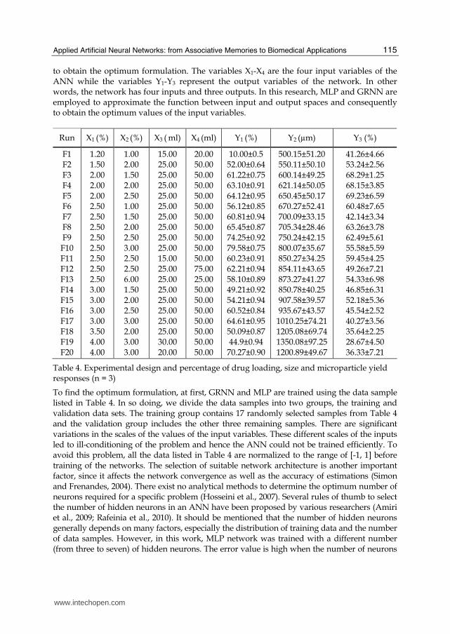
delivery systems such as microparticles, liposomes, nanocapsules, micellar systems and conjugates have become increasingly important, because these systems can overcome these pharmacokinetic problems, and maintain the pharmacological effect for an appropriate extended time. Controlled release therapeutic systems present some advantages over traditional pharmaceutical preparations due to the fact, less active drug is necessary for similar results and consequently less secondary effects are present (Dadashzadeh et al., 2008; Derakhshandeh et al., 2010a, 2010b, 2010c, 2010d). Since these systems are often polymeric and submicron in size, they can in general be used to provide targeted delivery (cellular/tissue) of drugs, to improve bioavailability, to sustain drug effect in target tissue, to solubilize drug for intravascular delivery and to improve the stability of therapeutic agents from enzymatic degradation (Derakhshandeh et al., 2010b). Sodium alginate as a biocompatible and biodegradable compound have lower toxicity compared to other polymers when taken orally and as a carrier could be suitable for encapsulation of drug. In this section, sodium alginate microparticle for oral delivery of furosemide was designed whether the encapsulation into microparticles might improve the oral absorption of this potent loop diuretic. To prepare an optimum formulation, MLP and GRNN are employed. The drug loaded formulation parameters are the input vectors of each network and are listed in Table 3. The microparticles drug loading (Y1), size of microspheres (Y2) and the amount of drug release in 2 h (Y3) constitute the output vector of GRNN and MLP. In this way, ANN was trained to investigate the functional dependence of input variables on the output response.

Factors Low level High level

X1 concentration of sodium alginate (%) 0.8 4

X2 concentration of CaCl2 (%) 1 6

X3 volume t of internal phase (ml) 15 30

X4 volume of external phase (ml) 20 75

Table 3. Factorial design parameters and experimental conditions.

Microspheres were prepared by ionotropic gelation technique (Chan et al., 2002). Sodium alginate was dissolved in distilled water with agitation to have different concentrations of 1.5 to 4% (w/v). The drug was added to aqueous solutions of sodium alginate and the solution was dropped using a hypodermic syringe into a second solution, containing CaCl2 with different concentration to cure for 15 min. After the microspheres formed, were separated, washed with distilled water, and dried in oven for 48 h. Based on preliminary study of the effect of parameters on the drug loading, size and preparation method yield of microparticle, 20 formulations were prepared. In vitro drug release study was carried out in USP XXII basket type dissolution test apparatus using Phosphate buffer solution (pH 7.4), simulated gastric fluid (SGF, pH 1.2) and simulated intestinal fluid (SIF, pH 7.4) as dissolution medium. Volume of dissolution medium was 500 ml and bath temperature was maintained at (37±10°C) throughout study. Basket speed was adjusted to 50 rpm. An interval of 1 hr, 5 ml of sample was withdrawn with replacement of fresh medium and analyzed for furosemide content by UV-Visible spectrophotometer at 273 nm. All the experimental units were analyzed in triplicate (n=3). At the end of this procedure, 20 formulations were prepared and are listed in Table 4. Indeed, the data of this table constitute the training and validation data sets which are used

www.intechopen.com


115

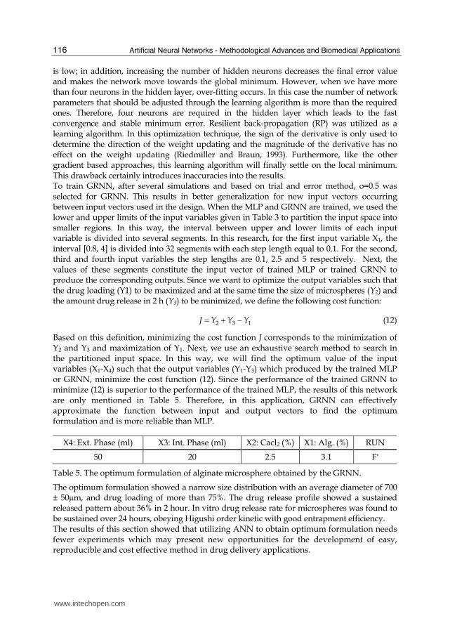
to obtain the optimum formulation. The variables X1-X4 are the four input variables of the ANN while the variables Y1-Y3 represent the output variables of the network. In other words, the network has four inputs and three outputs. In this research, MLP and GRNN are employed to approximate the function between input and output spaces and consequently to obtain the optimum values of the input variables.

Run X1 (%) X2 (%) X3 ( ml) X4 (ml) Y1 (%) Y2 (µm) Y3 (%)

F1 F2 F3 F4 F5 F6 F7 F8 F9 F10 F11 F12 F13 F14 F15 F16 F17 F18 F19 F20

1.20

1.50 2.00 2.00 2.00 2.50 2.50 2.50 2.50 2.50 2.50 2.50 2.50 3.00 3.00 3.00 3.00 3.50 4.00 4.00

1.00 2.00 1.50 2.00 2.50 1.00 1.50 2.00 2.50 3.00 2.50 2.50 6.00 1.50 2.00 2.50 3.00 2.00 3.00 3.00

15.00

25.00 25.00 25.00 25.00 25.00 25.00 25.00 25.00 25.00 15.00 25.00 25.00 25.00 25.00 25.00 25.00 25.00 30.00 20.00

20.00 50.00 50.00 50.00 50.00 50.00 50.00 50.00 50.00 50.00 50.00 75.00 25.00 50.00 50.00 50.00 50.00 50.00 50.00 50.00

10.00±0.5 52.00±0.6461.22±0.7563.10±0.9164.12±0.9556.12±0.8560.81±0.9465.45±0.8774.25±0.92

79.58±0.7560.23±0.9162.21±0.9458.10±0.8949.21±0.9254.21±0.9460.52±0.8464.61±0.9550.09±0.8744.9±0.94

70.27±0.90

500.15±51.20 550.11±50.10 600.14±49.25 621.14±50.05

650.45±50.17 670.27±52.41 700.09±33.15 705.34±28.46 750.24±42.15 800.07±35.67 850.27±34.25 854.11±43.65 873.27±41.27 850.78±40.25 907.58±39.57 935.67±43.57 1010.25±74.21 1205.08±69.74 1350.08±97.25 1200.89±49.67

41.26±4.66 53.24±2.56 68.29±1.25 68.15±3.85 69.23±6.59 60.48±7.65 42.14±3.34 63.26±3.78 62.49±5.61 55.58±5.59 59.45±4.25 49.26±7.21 54.33±6.98 46.85±6.31 52.18±5.36 45.54±2.52 40.27±3.56 35.64±2.25 28.67±4.50 36.33±7.21

Table 4. Experimental design and percentage of drug loading, size and microparticle yield responses (n = 3)

To find the optimum formulation, at first, GRNN and MLP are trained using the data sample listed in Table 4. In so doing, we divide the data samples into two groups, the training and validation data sets. The training group contains 17 randomly selected samples from Table 4 and the validation group includes the other three remaining samples. There are significant variations in the scales of the values of the input variables. These different scales of the inputs led to ill-conditioning of the problem and hence the ANN could not be trained efficiently. To avoid this problem, all the data listed in Table 4 are normalized to the range of [-1, 1] before training of the networks. The selection of suitable network architecture is another important factor, since it affects the network convergence as well as the accuracy of estimations (Simon and Frenandes, 2004). There exist no analytical methods to determine the optimum number of neurons required for a specific problem (Hosseini et al., 2007). Several rules of thumb to select the number of hidden neurons in an ANN have been proposed by various researchers (Amiri et al., 2009; Rafeinia et al., 2010). It should be mentioned that the number of hidden neurons generally depends on many factors, especially the distribution of training data and the number of data samples. However, in this work, MLP network was trained with a different number (from three to seven) of hidden neurons. The error value is high when the number of neurons

www.intechopen.com


116

is low; in addition, increasing the number of hidden neurons decreases the final error value and makes the network move towards the global minimum. However, when we have more than four neurons in the hidden layer, over-fitting occurs. In this case the number of network parameters that should be adjusted through the learning algorithm is more than the required ones. Therefore, four neurons are required in the hidden layer which leads to the fast convergence and stable minimum error. Resilient back-propagation (RP) was utilized as a learning algorithm. In this optimization technique, the sign of the derivative is only used to determine the direction of the weight updating and the magnitude of the derivative has no effect on the weight updating (Riedmiller and Braun, 1993). Furthermore, like the other gradient based approaches, this learning algorithm will finally settle on the local minimum. This drawback certainly introduces inaccuracies into the results. To train GRNN, after several simulations and based on trial and error method, σ=0.5 was selected for GRNN. This results in better generalization for new input vectors occurring between input vectors used in the design. When the MLP and GRNN are trained, we used the lower and upper limits of the input variables given in Table 3 to partition the input space into smaller regions. In this way, the interval between upper and lower limits of each input variable is divided into several segments. In this research, for the first input variable X1, the interval [0.8, 4] is divided into 32 segments with each step length equal to 0.1. For the second, third and fourth input variables the step lengths are 0.1, 2.5 and 5 respectively. Next, the values of these segments constitute the input vector of trained MLP or trained GRNN to produce the corresponding outputs. Since we want to optimize the output variables such that the drug loading (Y1) to be maximized and at the same time the size of microspheres (Y2) and the amount drug release in 2 h (Y3) to be minimized, we define the following cost function:

2 3 1J Y Y Y= + − (12)

Based on this definition, minimizing the cost function J corresponds to the minimization of Y2 and Y3 and maximization of Y1. Next, we use an exhaustive search method to search in the partitioned input space. In this way, we will find the optimum value of the input variables (X1-X4) such that the output variables (Y1-Y3) which produced by the trained MLP or GRNN, minimize the cost function (12). Since the performance of the trained GRNN to minimize (12) is superior to the performance of the trained MLP, the results of this network are only mentioned in Table 5. Therefore, in this application, GRNN can effectively approximate the function between input and output vectors to find the optimum formulation and is more reliable than MLP.

X4: Ext. Phase (ml) X3: Int. Phase (ml) X2: Cacl2 (%) X1: Alg. (%) RUN

50 20 2.5 3.1 F*

Table 5. The optimum formulation of alginate microsphere obtained by the GRNN.

The optimum formulation showed a narrow size distribution with an average diameter of 700 ± 50µm, and drug loading of more than 75%. The drug release profile showed a sustained released pattern about 36% in 2 hour. In vitro drug release rate for microspheres was found to be sustained over 24 hours, obeying Higushi order kinetic with good entrapment efficiency. The results of this section showed that utilizing ANN to obtain optimum formulation needs fewer experiments which may present new opportunities for the development of easy, reproducible and cost effective method in drug delivery applications.

www.intechopen.com


117

5. Conclusion

In this chapter, we provided a brief description of four types of ANNs including SFNN, GRNN, RBFN and MLP. Next, we investigated the diverse and innovative applications of these neural networks such as associative neural networks for recognition of analog and digital patterns, estimating the release profile of the betamethasone (BTM) and betamethasone acetate (BTMA) and optimizing the forusemide microcarrier formulation. Considering the first application, a hybrid model consists of SFNN in parallel with GRNN was proposed. SFNN is a simple recurrent neural network which has difficulty learning and storing analog and digital patterns as associative memories (Amiri et al., 2008). GRNN can find solutions for any given problem, but lack a recurrent structure to filter noise. Therefore, the hybrid model of SFNN and GRNN was proposed and a new one-shot learning algorithm for training the hybrid model put forwarded in the chapter. It was shown that this new hybrid model is able to perform essential properties found in associative memories such as generalization, completion and recognition of corrupted patterns. Moreover, a number of case studies were performed for the purpose of performance comparison between the hybrid model and others from different classes such as NDRAM, ART2 and Storkey. It was discussed that in comparison to classic associative memory models, the hybrid model has at least three significant advantages. First, the learning and recalling processes in the hybrid model are very short and efficient which make the hybrid model act much faster compared to the other networks. This is very helpful when either the dimensionality or the number of patterns to be stored is large, which results in significant reduction of computational time and cost. Second, more importantly the hybrid model does not have any spurious attractor. The third distinct feature is that the hybrid model not only realizes association of binary patterns but can also realize association of analog patterns without any preprocessing (Amiri et al., 2007, 2008, 2010). Consequently, we believe that this hybrid model constitutes a serious candidate for associative recall of analog and digital patterns which should be explored further in future studies. Regarding the biomedical application, the MLP, GRNN and RBFN are employed to model the release data and to predict the release profile of the BTM and the BTMA where in situ forming systems consist of poly (Lactide-co-glycolide), N-methyl-1-2-pyrolidon and ethyl heptanoat as a polymer, solvent and additive, respectively. Several simulations were presented to compare the potential of each neural network. NLPCA feature extraction technique was utilized to extract three features from each release graph, constituting the outputs of the neural network. By utilizing these three features, we converted and reduced the released graphs into three more effective values. Training the networks was carried out using L.O.O. cross-validation approach. This approach allows the training algorithm to use the entire data set for training and at the same time to test the performance of the trained network on new data which has not already seen by the network. It was demonstrated that the MLP as a data modeling tool, is more reliable and efficient tool than RBFN and GRNN, in order to estimate the release profile of BTM and BTMA drugs. Furthermore, we investigated the application of the GRNN and MLP for optimization of drug delivery system formulation. It would appear that performance of the trained GRNN to minimize the cost function is superior to the performance of the trained MLP. In this way, GRNN is promising to determine the optimum drug formulation. In sum, the application of the ANNs in biomedical research will definitely increase in the near future. However, the point which is noteworthy is the fact that there is no single modeling approach to address all requirements.

www.intechopen.com


118

6. Acknowledgements

The authors would like to thank Prof. Alireza Sadeghian, Prof. Sylvain Chartier, Prof. Simin Dadashzadeh, Dr. Mohammad Rafienia, and Mr. Hamed Davande for their insightful suggestions. We appreciate their assistance.

7. References

Amiri, M., Menhaj, M. B., & Fallah. A., (2007). Stability Analysis of self-feedback neural network structures, Amirkabir Journal of Science and Technology, 14(66A), 103-109.

Amiri, M., Davandeh, H., Sadeghian, A., & Seyyedsalehi, S.A., (2007). Auto-associative neural network based on new hybrid model of SFNN and GRNN. In Proceedings of the International Joint Conference on Neural Networks (IJCNN), 2664-2670, USA.

Amiri, M., Davandeh, H., Sadeghian, A., & Chartier, S., (2010) Feedback associative memory based on a new hybrid model of generalized regression and self-feedback neural networks, Neural Network, 23(7), 892-904.

Amiri, M., Menhaj, M. B., & Yazdanpanah, M.J. (2008a). A neural-network-based controller for a single-link flexible manipulator: comparison of FFNN and DRNN controllers. IEEE World Congress on Computational Intelligence (WCCI), 1687-92, Hong Kong.

Amiri M., Rafienia, M., Sadeghian A., (2009) Estimation of betamethasone release profiles from an in situ forming system based on the biodegradable polymer using artificial neural networks, IFMBE Proceedings, (2016-2019), Germany.

Amiri, M., Sadeghian, A., & Chartier, S., (2010) One-shot training algorithm for self feedback neural networks, Annual Conference of the North American Fuzzy Information Processing Society - NAFIPS , no. 5548272, Toronto, Canada.

Amiri, M., Saeb, S., Yazdanpanah, M.J., & Seyyedsalehi, S.A., (2008b). Analysis of the dynamical behavior of a feedback auto-associative memory. Neurocomputing, 71, 486-494.

Amiri, M., Bahrami, F. & Janahmadi, M. Functional modeling of astrocytes in epilepsy: a feedback system perspective, Neural Computing & Applications, DOI 10.1007/s00521-010-0479-0

Amrouche, A., & Rouvaen, J.M., (2006). Efficient system for speech recognition using general regression neural network. International Journal of Computer Systems Science and Engineering, 1(2), 183-189.

Atiya, A., & Abu-Mostafa, Y.S., (1993). An analog feedback associative memory. IEEE Transactions on Neural Networks, 2, 117-126.

Bégin, J., & Proulx, R., (1996). Categorization in unsupervised neural networks: The Eidos model. IEEE Transactions on Neural Networks, 7, 147-154.

Bing Yu , & Xingshi He (2006) Training Radial Basis Function Networks with Differential Evolution, Proceedings of World Academi of Science, Engineering and Technology, 11 , ISSN 1307-6884.

Brier, E., Zurada, J.M., & Aronoff G.R., (1995) Neural network predicted peak and trough of gentamicin concentrations. Pharm. Res. 12, 406–412.

Carpenter, G.A., & Grossberg, S., (2003) Adaptive resonance theory, In M.A. Arbib (Ed.), The Handbook of Brain Theory and Neural Networks, Second Edition, Cambridge, MA: MIT Press, 87-90.

Carpenter, G.A., & Grossberg, S., (1987) ART 2: Stable self-organization of pattern recognition codes for analog input patterns. Applied Optics, 26, 4919-4930.

www.intechopen.com


119

Chan L.W., Lee H.Y., Heng P.W.S. (2002). Production of alginate microspheres by internal gelation using an emulsification method. International Journal of Pharmaceutics, 242 , 259–260.

Chartier, S., & Proulx, R., (2005) NDRAM: Nonlinear dynamic recurrent associative memory for learning bipolar and nonbipolar correlated patterns, IEEE Transactions on Neural Networks, 16(6), 1393-1400.

Chartier, S., Boukadoum, M., & Amiri, M., (2009) BAM learning of nonlinearly separable tasks by using an asymmetrical output function and reinforcement learning, IEEE Transactions on Neural Networks, 20(8), 1281-1292.

Chen, T., & Chen. H., (1995) Universal approximation to nonlinear operators by neural networks with arbitrary activation functions and its application to dynamical system. IEEE Trans. Neural Networks 6, 911–917.

Cheng, K.S., Lin, J.S., & Mao, C.W., (1996) The application of competitive Hopfield neural network to medical image segmentation. IEEE Transactions on Medical Imaging, 15(4), 560-567.

Dadashzadeh S., Derakhshandeh K., Shirazi F.H., (2008) 9-Nitrocamptothecin polymeric nanoparticles: Cytotoxicity and pharmacokinetic studies of lactone and total forms of drug in rats. Anticancer Drugs, 19(8), 805-811.

Davande, H., Amiri, M., Sadeghian, A., & Chartier, S., (2008). Associative memory based on a new hybrid model of SFNN and GRNN: performance comparison with NDRAM, ART2 and MLP," IEEE World Congress on Computational Intelligence (WCCI), (1699-1704), Hong Kong.

Derakhshandeh K., Erfan M., Dadashzadeh S., (2007) Encapsulation of 9-nitrocamptothecin, a novel anticancer drug, in biodegradable nanoparticles: factorial design, characterization and release kinetics. Eur J Pharm biopharm 66, 34-41.

Derakhshandeh K., Dadashzadeh S., Soheili M., (2010a) Preparation and in vitro characterization of 9-nitrocamptothecin-loaded long circulating nanoparticles for delivery in cancer patients. International Journal of Nanomedicine. 463-471.

Derakhshandeh K., Fashi M., Seifoleslami S., (2010b) Thermosensitive Pluronic® hydrogel: prolonged injectable formulation for drug abuse. Drug Design, Development and Therapy, 4, 255-262.

Derakhshandeh K, Soleimani M., (2010c) Formulation and in vitro evaluation of nifedipine controlled release tablet: influence of combination of hydrophilic and hydrophobic matrix forms. Asian Journal of Pharmaceutics. in press.

Derakhshandeh K, Nikmohammadi M, Hosseinalizadeh A. (2010d) Factorial effect of process parameters on pharmaceutical characteristics of biodegradable PLGA microparticles. International Journal of Drug delivery. in press

Diederich, S., & Opper, M., (1987). Learning of correlated pattern in spin-glass networks by local learning rules. Physical Review Letter, 58, 949-952.

Freeman, J.A., (1993). Simulating neural networks with mathematica, 1st Ed. Addison-Wesley Longman Publishing Co., Inc.

Hopfield, J.J., (1982). Neural networks and physical systems with emergent collective computational abilities. Proceeding of Natural Academic Science, 79, 2554-2558.

Hosseini, S.M., Amiri, M., Najarian, S., & Dargahi, J. (2007) Application of artificial neural networks for the estimation of tumour characteristics in biological tissues, International Journal of Medical Robotics and Computer Assisted Surgery 3 (3), 235-244.

Hua A., Steven A. J., Melgardt M. D., Yuri M. L. (2003) Nano-encapsulation of furosemide microcrystals for controlled drug release. Journal of Controlled Release, 86, 59–62.

www.intechopen.com


120

Huang, Z., & Williamson, M.A., (1994) Geological pattern recognition and modeling with a general regression neural network. Canadian Journal of Exploration Geophysics, 30(1), 60-68.

Kamat HV, & Rao DH. (1995) Direct adaptive control of non-linear systems using a dynamic neural network. IEEE Transactions on Automatic Control. 39, 987–991.

Kanter, I., & Sompolinsky, H., (1987) Associative recall of memory without errors. Physical Review A, 35(1), 380-392.

Kramer, M.A. (1991) Nonlinear principal component analysis using auto-associative neural networks. AlChE J. 37,233–243.

Kubat, M. (1998) Decision Trees Can Initialize Radial-Basis Function Networks. IEEE Transactions Neural Networks, 813-821.

Ku, C.C., & Lee, K.Y., (1995) Diagonal recurrent neural network for dynamic system control. IEEE Transactions on Neural Networks, 6, 144-155.

Lim, C. P., Quek, S.S., & Peh, K.K. (2003) Prediction of drug release profiles using an intelligent learning system: an experimental study in transdermal iontophoresis. J. Pharma. Biomed. Anal. 31, 159–168.

Lindenberg, M., Kopp, S., Dressman B. (2004) Classification of orally administered drugs on the World Health Organization Model list of Essential Medicines according to the biopharmaceutics classification system. Eur J Pharm Biopharm, 58, 265-2782.

Mackay, J., Mensah GA, Mendis S, Greenlund K. The atlas of heart disease and stroke. Brighton: Myriad Edition Limited; 2004.

Moody, J., & Darken, C. (1991) Fast Learning Networks of Locally-Tuned Processing Units. Neural Computation. 579-588.

Rafienia, M., Amiri M., Janmaleki M., & Sadeghian A., (2010) Application of Artificial Neural Networks in controlled drug delivery Systems, Applied Artificial Intelligence. 24, 807–820.

Reznik, A., Galinskaya, A., Dekhtyarenko, O., & Nowicki, D. (2005). Preprocessing of matrix qcm sensors data for the classification by means of neural network. Sensors and Actuators B., 158-163.

Riedmiller, M., & Braun H., (1993) A direct adaptive method for faster backpropagation learning: the RPROP algorithm. IEEE Int. Conf. on Neural Networks 1, 586–591.

Robert, J., & Hewlett L.C.J. (2001) Radial Basis Function Networks 2: New Advances in Design. Simon, L., & Frenandes, M. (2004) Neural network-based prediction and optimization of

estradiol release from ethylene-vinyl acetate membranes. Comp. Chem. Eng. 28, 2407–2419.

Specht, D.E. (1991) A general regression neural network. IEEE Transactions on Neural Networks, 2(6), 568-576.

Storkey, A.J. & Valabregue, R., (1999) The basins of attraction of a new Hopfield learning rule. Neural Networks, 12, 869-876.

Takayama, K., Fujikawa, M., Obata, Y., & Morishita, M., (2003) Neural network based optimization of drug formulations. Adv. Drug Deliv. Rev. 55, 1217–1231.

Valafar, H., & Valafar, F., (1999) Prediction of a patient’s response to a specific drug treatment using artificial neural networks. IEEE 3694–3697.

Wachowiak, M.P., Elmaghraby, A.S., Smolikova, R., & Zurada, J.M., (2001). Generalized regression neural networks for biomedical image interpolation. Int. Joint Conf. on Neural Networks (IJCNN ), 2133-2138, USA.

www.intechopen.com

Artificial Neural Networks - Methodological Advances andBiomedical ApplicationsEdited by Prof. Kenji Suzuki

ISBN 978-953-307-243-2Hard cover, 362 pagesPublisher InTechPublished online 11, April, 2011Published in print edition April, 2011

InTech EuropeUniversity Campus STeP Ri Slavka Krautzeka 83/A 51000 Rijeka, Croatia Phone: +385 (51) 770 447 Fax: +385 (51) 686 166www.intechopen.com

InTech ChinaUnit 405, Office Block, Hotel Equatorial Shanghai No.65, Yan An Road (West), Shanghai, 200040, China

Phone: +86-21-62489820 Fax: +86-21-62489821

Artificial neural networks may probably be the single most successful technology in the last two decades whichhas been widely used in a large variety of applications in various areas. The purpose of this book is to providerecent advances of artificial neural networks in biomedical applications. The book begins with fundamentals ofartificial neural networks, which cover an introduction, design, and optimization. Advanced architectures forbiomedical applications, which offer improved performance and desirable properties, follow. Parts continuewith biological applications such as gene, plant biology, and stem cell, medical applications such as skindiseases, sclerosis, anesthesia, and physiotherapy, and clinical and other applications such as clinicaloutcome, telecare, and pre-med student failure prediction. Thus, this book will be a fundamental source ofrecent advances and applications of artificial neural networks in biomedical areas. The target audienceincludes professors and students in engineering and medical schools, researchers and engineers inbiomedical industries, medical doctors, and healthcare professionals.

How to referenceIn order to correctly reference this scholarly work, feel free to copy and paste the following:

Mahmood Amiri and Katayoun Derakhshandeh (2011). Applied Artificial Neural Networks: from AssociativeMemories to Biomedical Applications, Artificial Neural Networks - Methodological Advances and BiomedicalApplications, Prof. Kenji Suzuki (Ed.), ISBN: 978-953-307-243-2, InTech, Available from:http://www.intechopen.com/books/artificial-neural-networks-methodological-advances-and-biomedical-applications/applied-artificial-neural-networks-from-associative-memories-to-biomedical-applications

© 2011 The Author(s). Licensee IntechOpen. This chapter is distributedunder the terms of the Creative Commons Attribution-NonCommercial-ShareAlike-3.0 License, which permits use, distribution and reproduction fornon-commercial purposes, provided the original is properly cited andderivative works building on this content are distributed under the samelicense.

https://creativecommons.org/licenses/by-nc-sa/3.0/

applied artificial neural networks: from associative memories to

Documents