arti cial intelligence - fai.cs.uni-saarland.de · introduction minimax search evaluation fns...
TRANSCRIPT
Introduction Minimax Search Evaluation Fns Alpha-Beta Search MCTS Conclusion References
Artificial Intelligence6. Adversarial Search
What To Do When Your “Solution” is Somebody Else’s Failure
Alvaro Torralba Wolfgang Wahlster
Summer Term 2018
Thanks to Prof. Hoffmann for slide sources
Torralba and Wahlster Artificial Intelligence Chapter 6: Adversarial Search 1/58
Introduction Minimax Search Evaluation Fns Alpha-Beta Search MCTS Conclusion References
Agenda
1 Introduction
2 Minimax Search
3 Evaluation Functions
4 Alpha-Beta Search
5 Monte-Carlo Tree Search (MCTS)
6 Conclusion
Torralba and Wahlster Artificial Intelligence Chapter 6: Adversarial Search 2/58
Introduction Minimax Search Evaluation Fns Alpha-Beta Search MCTS Conclusion References
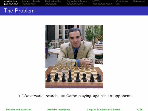
The Problem
→ ”Adversarial search” = Game playing against an opponent.
Torralba and Wahlster Artificial Intelligence Chapter 6: Adversarial Search 4/58
Introduction Minimax Search Evaluation Fns Alpha-Beta Search MCTS Conclusion References
Why AI Game Playing?
Many good reasons:
Playing a game well clearly requires a form of “intelligence”.
Games capture a pure form of competition between opponents.
Games are abstract and precisely defined, thus very easy toformalize.
→ Game playing is one of the oldest sub-areas of AI (ca. 1950).
→ The dream of a machine that plays Chess is, indeed, much older thanAI! (von Kempelen’s “Schachturke” (1769), Torres y Quevedo’s “ElAjedrecista” (1912))
Torralba and Wahlster Artificial Intelligence Chapter 6: Adversarial Search 5/58

Introduction Minimax Search Evaluation Fns Alpha-Beta Search MCTS Conclusion References
“Game” Playing? Which Games?
. . . sorry, we’re not gonna do football here.
Restrictions:
Game states discrete, number of game states finite.
Finite number of possible moves.
The game state is fully observable.
The outcome of each move is deterministic.
Two players: Max and Min.
Turn-taking: It’s each player’s turn alternatingly. Max begins.
Terminal game states have a utility u. Max tries to maximize u, Mintries to minimize u.
In that sense, the utility for Min is the exact opposite of the utilityfor Max (“zero-sum”).
There are no infinite runs of the game (no matter what moves arechosen, a terminal state is reached after a finite number of steps).
Torralba and Wahlster Artificial Intelligence Chapter 6: Adversarial Search 6/58
Introduction Minimax Search Evaluation Fns Alpha-Beta Search MCTS Conclusion References
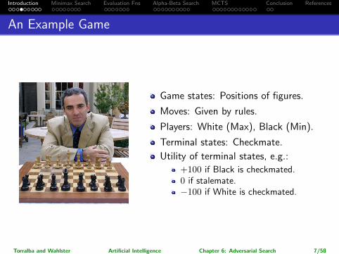
An Example Game
Game states: Positions of figures.
Moves: Given by rules.
Players: White (Max), Black (Min).
Terminal states: Checkmate.
Utility of terminal states, e.g.:
+100 if Black is checkmated.0 if stalemate.−100 if White is checkmated.
Torralba and Wahlster Artificial Intelligence Chapter 6: Adversarial Search 7/58

Introduction Minimax Search Evaluation Fns Alpha-Beta Search MCTS Conclusion References
“Game” Playing? Which Games Not?
. . . football.
Important types of games that we don’t tackle here:
Chance. (E.g., backgammon)
More than two players. (E.g., halma)
Hidden information. (E.g., most card games)
Simultaneous moves. (E.g., football)
Not zero-sum, i.e., outcomes may be beneficial (or detrimental) forboth players. (→ Game theory: Auctions, elections, economy,politics, . . . )
→ Many of these more general game types can be handled bysimilar/extended algorithms.
Torralba and Wahlster Artificial Intelligence Chapter 6: Adversarial Search 8/58
Introduction Minimax Search Evaluation Fns Alpha-Beta Search MCTS Conclusion References
(A Brief Note On) Formalization
Definition (Game State Space). A game state space is a 6-tupleΘ = (S,A, T, I, ST , u) where:
S, A, T , I: States, actions, deterministic transition relation, initialstate. As in classical search problems, except:
S is the disjoint union of SMax, SMin, and ST .A is the disjoint union of AMax and AMin.For a ∈ AMax, if s
a−→ s′ then s ∈ SMax and s′ ∈ SMin ∪ ST .For a ∈ AMin, if s
a−→ s′ then s ∈ SMin and s′ ∈ SMax ∪ ST .ST is the set of terminal states.
u : ST 7→ R is the utility function.
Commonly used terminology: state=position, terminal state=endstate, action=move.
(A round of the game – one move Max, one move Min – is often referred to asa “move”, and individual actions as “half-moves”. We don’t do that here.)
Torralba and Wahlster Artificial Intelligence Chapter 6: Adversarial Search 9/58
Introduction Minimax Search Evaluation Fns Alpha-Beta Search MCTS Conclusion References
Why Games are Hard to Solve
Why Games are hard to solve, part 1: → What is a “solution” here?
Definition (Strategy). Let Θ be a game state space, and let X ∈ {Max,Min}. A strategy for X is a function σX : SX 7→ AX so that a is applicable tos whenever σX(s) = a.
We don’t know how the opponent will react, and need to prepare for allpossibilities.
A strategy is optimal if it yields the best possible utility for X assumingperfect opponent play (not formalized here).
In (almost) all games, computing a strategy is infeasible. Instead, computethe next move “on demand”, given the current game state.
Why Games are hard to solve, part 2:
Number of reachable states: in Chess 1040; in Go 10100.
It’s worse even: Our algorithms here look at search trees (game trees), noduplicate checking. Chess: branching factor ca. 35, ca. 100 moves≈ 10154. Go: branching factor ca. 200, ca. 300 moves ≈ 10690.
Torralba and Wahlster Artificial Intelligence Chapter 6: Adversarial Search 10/58
Introduction Minimax Search Evaluation Fns Alpha-Beta Search MCTS Conclusion References
Our Agenda for This Chapter
Minimax Search: How to compute an optimal strategy?
→ Minimax is the canonical (and easiest to understand) algorithm forsolving games, i.e., computing an optimal strategy.
Evaluation Functions: But what if we don’t have the time/memory tosolve the entire game?
→ Given limited time, the best we can do is look ahead as far as possible.Evaluation functions tell us how to evaluate the leaf states at the cut-off.
Alpha-Beta Search: How to prune unnecessary parts of the tree?
→ An essential improvement over Minimax.
Monte-Carlo Tree Search (MCTS): An alternative form of game search,based on sampling rather than exhaustive enumeration.
→ The main alternative to Alpha-Beta Search.
→ Alpha-Beta = state of the art in Chess, MCTS = state of the art in Go.
Torralba and Wahlster Artificial Intelligence Chapter 6: Adversarial Search 11/58
Introduction Minimax Search Evaluation Fns Alpha-Beta Search MCTS Conclusion References
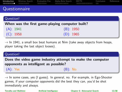
Questionnaire
Question!
When was the first game-playing computer built?
(A): 1941
(C): 1958
(B): 1950
(D): 1965
→ In 1941, a small box beat humans at Nim (take away objects from heaps,player taking the last object looses).
Question!
Does the video game industry attempt to make the computeropponents as intelligent as possible?
(A): Yes (B): No
→ In some cases, yes (I guess). In general, no. For example, in Ego-Shootergames, if your computer opponents did the best they can, you’d be shotimmediately and always.
Torralba and Wahlster Artificial Intelligence Chapter 6: Adversarial Search 12/58
Introduction Minimax Search Evaluation Fns Alpha-Beta Search MCTS Conclusion References
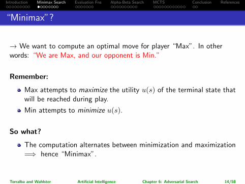
“Minimax”?
→ We want to compute an optimal move for player “Max”. In otherwords: “We are Max, and our opponent is Min.”
Remember:
Max attempts to maximize the utility u(s) of the terminal state thatwill be reached during play.
Min attempts to minimize u(s).
So what?
The computation alternates between minimization and maximization=⇒ hence “Minimax”.
Torralba and Wahlster Artificial Intelligence Chapter 6: Adversarial Search 14/58
Introduction Minimax Search Evaluation Fns Alpha-Beta Search MCTS Conclusion References
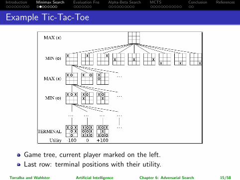
Example Tic-Tac-Toe
Game tree, current player marked on the left.
Last row: terminal positions with their utility.
Torralba and Wahlster Artificial Intelligence Chapter 6: Adversarial Search 15/58
Introduction Minimax Search Evaluation Fns Alpha-Beta Search MCTS Conclusion References
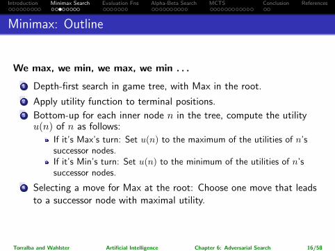
Minimax: Outline
We max, we min, we max, we min . . .
1 Depth-first search in game tree, with Max in the root.
2 Apply utility function to terminal positions.3 Bottom-up for each inner node n in the tree, compute the utilityu(n) of n as follows:
If it’s Max’s turn: Set u(n) to the maximum of the utilities of n’ssuccessor nodes.If it’s Min’s turn: Set u(n) to the minimum of the utilities of n’ssuccessor nodes.
4 Selecting a move for Max at the root: Choose one move that leadsto a successor node with maximal utility.
Torralba and Wahlster Artificial Intelligence Chapter 6: Adversarial Search 16/58
Introduction Minimax Search Evaluation Fns Alpha-Beta Search MCTS Conclusion References
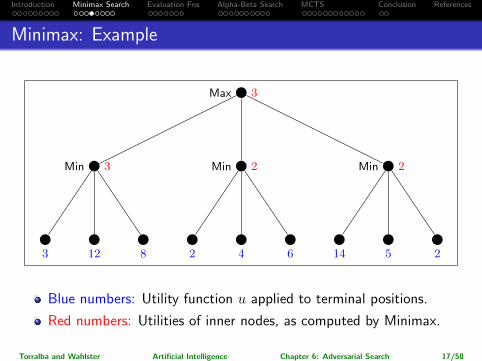
Minimax: Example
Max 3
Min 3
3 12 8
Min 2
2 4 6
Min 2
14 5 2
Blue numbers: Utility function u applied to terminal positions.
Red numbers: Utilities of inner nodes, as computed by Minimax.
Torralba and Wahlster Artificial Intelligence Chapter 6: Adversarial Search 17/58

Introduction Minimax Search Evaluation Fns Alpha-Beta Search MCTS Conclusion References
Minimax: Pseudo-Code
Input: State s ∈ SMax, in which Max is to move.
function Minimax-Decision(s) returns an actionv ← Max-Value(s)return an action a ∈ Actions(s) yielding value v
function Max-Value(s) returns a utility valueif Terminal-Test(s) then return u(s)v ← −∞for each a ∈ Actions(s) dov ← max(v,Min-Value(ChildState(s, a)))
return v
function Min-Value(s) returns a utility valueif Terminal-Test(s) then return u(s)v ← +∞for each a ∈ Actions(s) dov ← min(v,Max-Value(ChildState(s, a)))
return v
Torralba and Wahlster Artificial Intelligence Chapter 6: Adversarial Search 18/58
Introduction Minimax Search Evaluation Fns Alpha-Beta Search MCTS Conclusion References
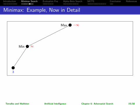
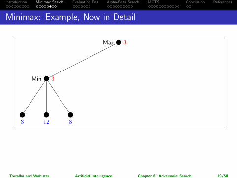
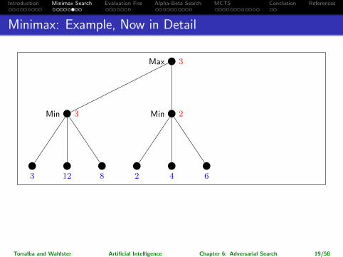
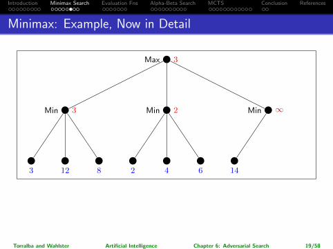
Minimax: Example, Now in Detail
Max −∞
Max 3
Min ∞
Min 3
3
12 8
Min ∞Min 2
2 4 6
Min ∞Min 14Min 5Min 2
14 5 2
→ So which action for Max is returned?
Leftmost branch.
Note: The maximalpossible pay-off is higher for the rightmost branch, but assuming perfect play ofMin, it’s better to go left. (Going right would be “relying on your opponent todo something stupid”.)
Torralba and Wahlster Artificial Intelligence Chapter 6: Adversarial Search 19/58
Introduction Minimax Search Evaluation Fns Alpha-Beta Search MCTS Conclusion References
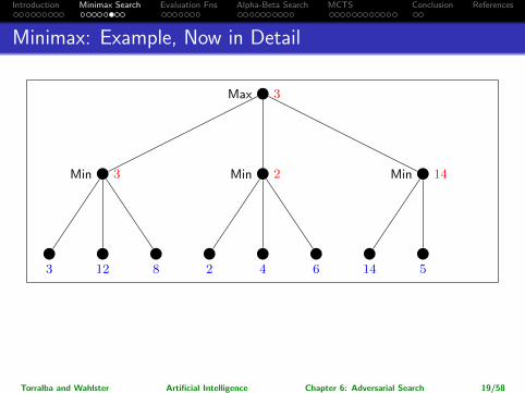
Minimax: Example, Now in Detail
Max −∞
Max 3
Min ∞
Min 3
3 12 8
Min ∞Min 2
2 4 6
Min ∞Min 14Min 5Min 2
14 5 2
→ So which action for Max is returned?
Leftmost branch.
Note: The maximalpossible pay-off is higher for the rightmost branch, but assuming perfect play ofMin, it’s better to go left. (Going right would be “relying on your opponent todo something stupid”.)
Torralba and Wahlster Artificial Intelligence Chapter 6: Adversarial Search 19/58

Introduction Minimax Search Evaluation Fns Alpha-Beta Search MCTS Conclusion References
Minimax: Example, Now in Detail
Max −∞
Max 3
Min ∞
Min 3
3 12 8
Min ∞
Min 2
2
4 6
Min ∞Min 14Min 5Min 2
14 5 2
→ So which action for Max is returned?
Leftmost branch.
Note: The maximalpossible pay-off is higher for the rightmost branch, but assuming perfect play ofMin, it’s better to go left. (Going right would be “relying on your opponent todo something stupid”.)
Torralba and Wahlster Artificial Intelligence Chapter 6: Adversarial Search 19/58
Introduction Minimax Search Evaluation Fns Alpha-Beta Search MCTS Conclusion References
Minimax: Example, Now in Detail
Max −∞
Max 3
Min ∞
Min 3
3 12 8
Min ∞
Min 2
2 4 6
Min ∞Min 14Min 5Min 2
14 5 2
→ So which action for Max is returned?
Leftmost branch.
Note: The maximalpossible pay-off is higher for the rightmost branch, but assuming perfect play ofMin, it’s better to go left. (Going right would be “relying on your opponent todo something stupid”.)
Torralba and Wahlster Artificial Intelligence Chapter 6: Adversarial Search 19/58
Introduction Minimax Search Evaluation Fns Alpha-Beta Search MCTS Conclusion References
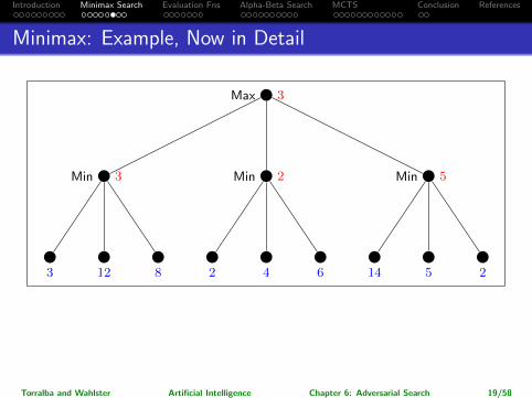
Minimax: Example, Now in Detail
Max −∞
Max 3
Min ∞
Min 3
3 12 8
Min ∞
Min 2
2 4 6
Min ∞
Min 14Min 5Min 2
14
5 2
→ So which action for Max is returned?
Leftmost branch.
Note: The maximalpossible pay-off is higher for the rightmost branch, but assuming perfect play ofMin, it’s better to go left. (Going right would be “relying on your opponent todo something stupid”.)
Torralba and Wahlster Artificial Intelligence Chapter 6: Adversarial Search 19/58
Introduction Minimax Search Evaluation Fns Alpha-Beta Search MCTS Conclusion References
Minimax: Example, Now in Detail
Max −∞
Max 3
Min ∞
Min 3
3 12 8
Min ∞
Min 2
2 4 6
Min ∞
Min 14
Min 5Min 2
14 5
2
→ So which action for Max is returned?
Leftmost branch.
Note: The maximalpossible pay-off is higher for the rightmost branch, but assuming perfect play ofMin, it’s better to go left. (Going right would be “relying on your opponent todo something stupid”.)
Torralba and Wahlster Artificial Intelligence Chapter 6: Adversarial Search 19/58
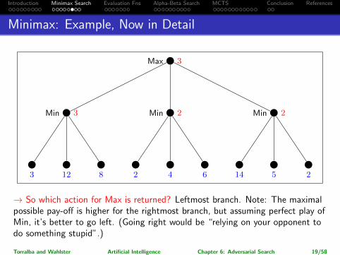
Introduction Minimax Search Evaluation Fns Alpha-Beta Search MCTS Conclusion References
Minimax: Example, Now in Detail
Max −∞
Max 3
Min ∞
Min 3
3 12 8
Min ∞
Min 2
2 4 6
Min ∞Min 14
Min 5
Min 2
14 5 2
→ So which action for Max is returned?
Leftmost branch.
Note: The maximalpossible pay-off is higher for the rightmost branch, but assuming perfect play ofMin, it’s better to go left. (Going right would be “relying on your opponent todo something stupid”.)
Torralba and Wahlster Artificial Intelligence Chapter 6: Adversarial Search 19/58
Introduction Minimax Search Evaluation Fns Alpha-Beta Search MCTS Conclusion References
Minimax: Example, Now in Detail
Max −∞
Max 3
Min ∞
Min 3
3 12 8
Min ∞
Min 2
2 4 6
Min ∞Min 14Min 5
Min 2
14 5 2
→ So which action for Max is returned? Leftmost branch. Note: The maximalpossible pay-off is higher for the rightmost branch, but assuming perfect play ofMin, it’s better to go left. (Going right would be “relying on your opponent todo something stupid”.)
Torralba and Wahlster Artificial Intelligence Chapter 6: Adversarial Search 19/58
Introduction Minimax Search Evaluation Fns Alpha-Beta Search MCTS Conclusion References
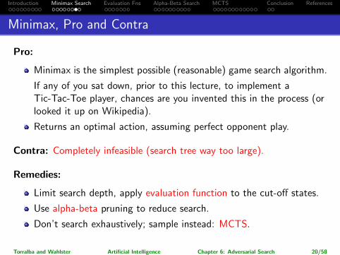
Minimax, Pro and Contra
Pro:
Minimax is the simplest possible (reasonable) game search algorithm.
If any of you sat down, prior to this lecture, to implement aTic-Tac-Toe player, chances are you invented this in the process (orlooked it up on Wikipedia).
Returns an optimal action, assuming perfect opponent play.
Contra: Completely infeasible (search tree way too large).
Remedies:
Limit search depth, apply evaluation function to the cut-off states.
Use alpha-beta pruning to reduce search.
Don’t search exhaustively; sample instead: MCTS.
Torralba and Wahlster Artificial Intelligence Chapter 6: Adversarial Search 20/58

Introduction Minimax Search Evaluation Fns Alpha-Beta Search MCTS Conclusion References
Questionnaire
Tic Tac Toe.
Max = x, Min = o.
Max wins: u = 100; Min wins: u = −100;stalemate: u = 0.
Question!
What’s the Minimax value for the state shown above? (Note:Max to move)
(A): 100 (B): −100
→ 100: Max moves; choosing the top left corner, it’s a certain win for Max.
Question!
What’s the Minimax value for the initial game state?
(A): 100 (B): −100
→ The correct value (and thus the value computed by Minimax) is 0: Given perfectplay, Tic Tac Toe always results in a stalemate. (Seen “War Games”, anybody?)
Torralba and Wahlster Artificial Intelligence Chapter 6: Adversarial Search 21/58

Introduction Minimax Search Evaluation Fns Alpha-Beta Search MCTS Conclusion References
Evaluation Functions
Problem: Minimax game tree too big.
Solution: Impose a search depth limit (“horizon”) d, and apply anevaluation function to the non-terminal cut-off states.
An evaluation function f maps game states to numbers:
f(s) is an estimate of the actual value of s (as would be computedby unlimited-depth Minimax for s).→ If cut-off state is terminal: Use actual utility u instead of f .
Analogy to heuristic functions (cf. Chapter 5): We want f to beboth (a) accurate and (b) fast.
Another analogy: (a) and (b) are in contradiction . . . need totrade-off accuracy against overhead.
→ Most games (e.g. Chess): f inaccurate but very fast. AlphaGo:f accurate but slow.
Torralba and Wahlster Artificial Intelligence Chapter 6: Adversarial Search 23/58
Introduction Minimax Search Evaluation Fns Alpha-Beta Search MCTS Conclusion References
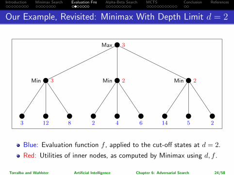
Our Example, Revisited: Minimax With Depth Limit d = 2
Max 3
Min 3
3 12 8
Min 2
2 4 6
Min 2
14 5 2
Blue: Evaluation function f , applied to the cut-off states at d = 2.
Red: Utilities of inner nodes, as computed by Minimax using d, f .
Torralba and Wahlster Artificial Intelligence Chapter 6: Adversarial Search 24/58
Introduction Minimax Search Evaluation Fns Alpha-Beta Search MCTS Conclusion References
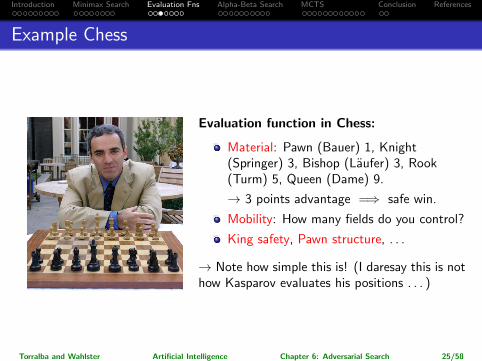
Example Chess
Evaluation function in Chess:
Material: Pawn (Bauer) 1, Knight(Springer) 3, Bishop (Laufer) 3, Rook(Turm) 5, Queen (Dame) 9.
→ 3 points advantage =⇒ safe win.
Mobility: How many fields do you control?
King safety, Pawn structure, . . .
→ Note how simple this is! (I daresay this is nothow Kasparov evaluates his positions . . . )
Torralba and Wahlster Artificial Intelligence Chapter 6: Adversarial Search 25/58
Introduction Minimax Search Evaluation Fns Alpha-Beta Search MCTS Conclusion References
Linear Evaluation Functions, Search Depth
Fast simple f : weighted linear function
w1f1 + w2f2 + · · ·+ wnfn
where the wi are the weights, and the fi are the features.
How to obtain such functions?
Weights wi can be learned automatically.
The features fi have to be designed by human experts.
And how deeply to search?
Iterative deepening until time for move is up.
Better: quiescence search, dynamically adapt depth limit, searchdeeper in “unquiet” positions (e.g. Chess piece exchange situations).
Torralba and Wahlster Artificial Intelligence Chapter 6: Adversarial Search 26/58
Introduction Minimax Search Evaluation Fns Alpha-Beta Search MCTS Conclusion References
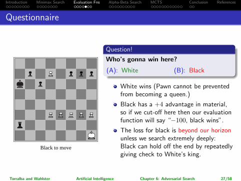
Questionnaire
Black to move
Question!
Who’s gonna win here?
(A): White (B): Black
White wins (Pawn cannot be preventedfrom becoming a queen.)
Black has a +4 advantage in material,so if we cut-off here then our evaluationfunction will say “−100, black wins”.
The loss for black is beyond our horizonunless we search extremely deeply:Black can hold off the end by repeatedlygiving check to White’s king.
Torralba and Wahlster Artificial Intelligence Chapter 6: Adversarial Search 27/58

Introduction Minimax Search Evaluation Fns Alpha-Beta Search MCTS Conclusion References
Questionnaire, ctd.
Tic-Tac-Toe. Max = x, Min = o.
Evaluation function f1(s): Number of rows,columns, and diagonals that contain ATLEAST ONE “x”.
(d: depth limit; I: initial state)
Question!
With d = 3 i.e. considering the moves Max-Min-Max, and using f1,which moves may Minimax choose for Max in the initial state I?
(A): Middle. (B): Corner.
→ (A): Alone, an “x” in the middle gives f1 = 4, and an “x” in the corner givesf1 = 3. If Max chooses a corner, then Min may choose the middle and themaximum reachable in the next step is f1 = 5. If Max chooses the middle,wherever Min moves, Max can choose a corner afterwards and get f1 = 6.
Torralba and Wahlster Artificial Intelligence Chapter 6: Adversarial Search 28/58
Introduction Minimax Search Evaluation Fns Alpha-Beta Search MCTS Conclusion References
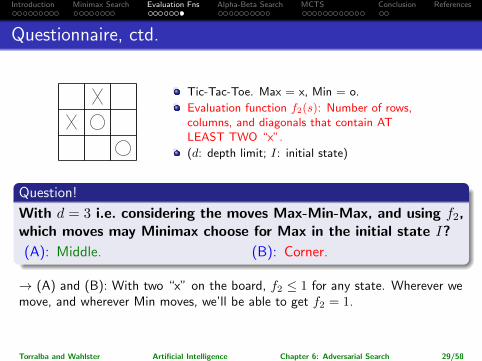
Questionnaire, ctd.
Tic-Tac-Toe. Max = x, Min = o.
Evaluation function f2(s): Number of rows,columns, and diagonals that contain ATLEAST TWO “x”.
(d: depth limit; I: initial state)
Question!
With d = 3 i.e. considering the moves Max-Min-Max, and using f2,which moves may Minimax choose for Max in the initial state I?
(A): Middle. (B): Corner.
→ (A) and (B): With two “x” on the board, f2 ≤ 1 for any state. Wherever wemove, and wherever Min moves, we’ll be able to get f2 = 1.
Torralba and Wahlster Artificial Intelligence Chapter 6: Adversarial Search 29/58

Introduction Minimax Search Evaluation Fns Alpha-Beta Search MCTS Conclusion References
Alpha Pruning: Idea
Max (A)
Maxvalue: m
Minvalue: n
Min (B)
Say n > m.
→ By choosing to go to the left in Maxnode (A), Max already can get utility atleast n in this part of the game.
Say that, “later on in the same sub-tree”, i.e. below a different childnodeof (A), in Min node (B) Min can forceMax to get value m < n.
Then we already know that (B) will notactually be reached during the game,given the strategy we currently computefor Max.
Torralba and Wahlster Artificial Intelligence Chapter 6: Adversarial Search 31/58

Introduction Minimax Search Evaluation Fns Alpha-Beta Search MCTS Conclusion References
Alpha Pruning: The Idea in Our Example
Question:
Can we save somework here?
Max 3
Min 3
3 12 8
Min 2
2 4 6
Min 2
14 5 2
Max ≥ 3
Min 3
3 12 8
Min ≤ 2
2
Min
Answer: Yes!
→ We alreadyknow at thispoint that themiddle actionwon’t be takenby Max.
Torralba and Wahlster Artificial Intelligence Chapter 6: Adversarial Search 32/58
Introduction Minimax Search Evaluation Fns Alpha-Beta Search MCTS Conclusion References
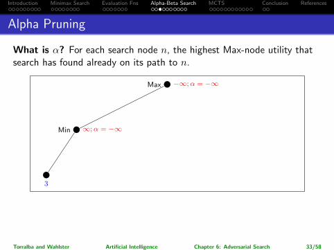
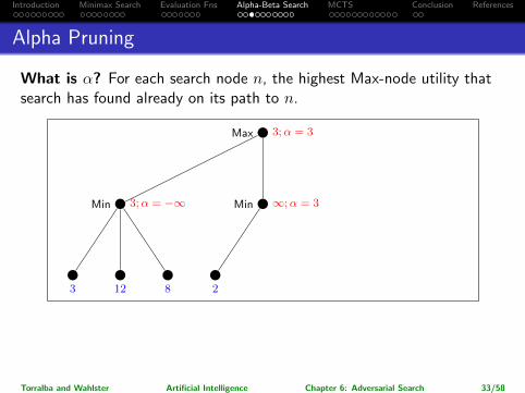
Alpha Pruning
What is α? For each search node n, the highest Max-node utility thatsearch has found already on its path to n.
Max −∞;α = −∞
Max 3;α = 3
Min ∞;α = −∞
Min 3;α = −∞
3
12 8
Min ∞;α = 3Min 2;α = 3
2
Min
How to use α? In a Min node n, if one of the successors already hasutility ≤ α, then stop considering n. (Pruning out its remainingsuccessors.)
Torralba and Wahlster Artificial Intelligence Chapter 6: Adversarial Search 33/58

Introduction Minimax Search Evaluation Fns Alpha-Beta Search MCTS Conclusion References
Alpha Pruning
What is α? For each search node n, the highest Max-node utility thatsearch has found already on its path to n.
Max −∞;α = −∞
Max 3;α = 3
Min ∞;α = −∞
Min 3;α = −∞
3 12 8
Min ∞;α = 3Min 2;α = 3
2
Min
How to use α? In a Min node n, if one of the successors already hasutility ≤ α, then stop considering n. (Pruning out its remainingsuccessors.)
Torralba and Wahlster Artificial Intelligence Chapter 6: Adversarial Search 33/58
Introduction Minimax Search Evaluation Fns Alpha-Beta Search MCTS Conclusion References
Alpha Pruning
What is α? For each search node n, the highest Max-node utility thatsearch has found already on its path to n.
Max −∞;α = −∞
Max 3;α = 3
Min ∞;α = −∞
Min 3;α = −∞
3 12 8
Min ∞;α = 3
Min 2;α = 3
2
Min
How to use α? In a Min node n, if one of the successors already hasutility ≤ α, then stop considering n. (Pruning out its remainingsuccessors.)
Torralba and Wahlster Artificial Intelligence Chapter 6: Adversarial Search 33/58
Introduction Minimax Search Evaluation Fns Alpha-Beta Search MCTS Conclusion References
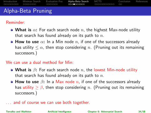
Alpha-Beta Pruning
Reminder:
What is α: For each search node n, the highest Max-node utilitythat search has found already on its path to n.
How to use α: In a Min node n, if one of the successors alreadyhas utility ≤ α, then stop considering n. (Pruning out its remainingsuccessors.)
We can use a dual method for Min:
What is β: For each search node n, the lowest Min-node utilitythat search has found already on its path to n.
How to use β: In a Max node n, if one of the successors alreadyhas utility ≥ β, then stop considering n. (Pruning out its remainingsuccessors.)
. . . and of course we can use both together.
Torralba and Wahlster Artificial Intelligence Chapter 6: Adversarial Search 34/58
Introduction Minimax Search Evaluation Fns Alpha-Beta Search MCTS Conclusion References
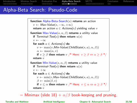
Alpha-Beta Search: Pseudo-Code
function Alpha-Beta-Search(s) returns an actionv ← Max-Value(s,−∞,+∞)return an action a ∈ Actions(s) yielding value v
function Max-Value(s, α, β) returns a utility valueif Terminal-Test(s) then return u(s)v ← −∞for each a ∈ Actions(s) dov ← max(v,Min-Value(ChildState(s, a), α, β))α ← max(α, v)if v ≥ β then return v /* Here: v ≥ β ⇔ α ≥ β */
return v
function Min-Value(s, α, β) returns a utility valueif Terminal-Test(s) then return u(s)v ← +∞for each a ∈ Actions(s) dov ← min(v,Max-Value(ChildState(s, a), α, β))β ← min(β, v)if v ≤ α then return v /* Here: v ≤ α⇔ α ≥ β */
return v
= Minimax (slide 18) + α/β book-keeping and pruning.
Torralba and Wahlster Artificial Intelligence Chapter 6: Adversarial Search 35/58
Introduction Minimax Search Evaluation Fns Alpha-Beta Search MCTS Conclusion References
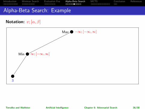
Alpha-Beta Search: Example
Notation: v; [α, β]
Max −∞; [−∞,∞]
Max 3; [3,∞]
Min ∞; [−∞,∞]
Min 3; [−∞, 3]
3
12 8
Min ∞; [3,∞]Min 2; [3, 2]
2
Min ∞; [3,∞]Min 14; [3, 14]Min 5; [3, 5]Min 2; [3, 2]
14 5 2
→ Note: We could have saved work by choosing the opposite order for thesuccessors of the rightmost Min node. Choosing the best moves (for each ofMax and Min) first yields more pruning!
Torralba and Wahlster Artificial Intelligence Chapter 6: Adversarial Search 36/58
Introduction Minimax Search Evaluation Fns Alpha-Beta Search MCTS Conclusion References
Alpha-Beta Search: Example
Notation: v; [α, β]
Max −∞; [−∞,∞]
Max 3; [3,∞]
Min ∞; [−∞,∞]
Min 3; [−∞, 3]
3 12 8
Min ∞; [3,∞]
Min 2; [3, 2]
2
Min ∞; [3,∞]Min 14; [3, 14]Min 5; [3, 5]Min 2; [3, 2]
14 5 2
→ Note: We could have saved work by choosing the opposite order for thesuccessors of the rightmost Min node. Choosing the best moves (for each ofMax and Min) first yields more pruning!
Torralba and Wahlster Artificial Intelligence Chapter 6: Adversarial Search 36/58
Introduction Minimax Search Evaluation Fns Alpha-Beta Search MCTS Conclusion References
Alpha-Beta Search: Example
Notation: v; [α, β]
Max −∞; [−∞,∞]
Max 3; [3,∞]
Min ∞; [−∞,∞]
Min 3; [−∞, 3]
3 12 8
Min ∞; [3,∞]
Min 2; [3, 2]
2
Min ∞; [3,∞]
Min 14; [3, 14]Min 5; [3, 5]Min 2; [3, 2]
14
5 2
→ Note: We could have saved work by choosing the opposite order for thesuccessors of the rightmost Min node. Choosing the best moves (for each ofMax and Min) first yields more pruning!
Torralba and Wahlster Artificial Intelligence Chapter 6: Adversarial Search 36/58
Introduction Minimax Search Evaluation Fns Alpha-Beta Search MCTS Conclusion References
Alpha-Beta Search: Example
Notation: v; [α, β]
Max −∞; [−∞,∞]
Max 3; [3,∞]
Min ∞; [−∞,∞]
Min 3; [−∞, 3]
3 12 8
Min ∞; [3,∞]
Min 2; [3, 2]
2
Min ∞; [3,∞]
Min 14; [3, 14]
Min 5; [3, 5]Min 2; [3, 2]
14 5
2
→ Note: We could have saved work by choosing the opposite order for thesuccessors of the rightmost Min node. Choosing the best moves (for each ofMax and Min) first yields more pruning!
Torralba and Wahlster Artificial Intelligence Chapter 6: Adversarial Search 36/58

Introduction Minimax Search Evaluation Fns Alpha-Beta Search MCTS Conclusion References
Alpha-Beta Search: Example
Notation: v; [α, β]
Max −∞; [−∞,∞]
Max 3; [3,∞]
Min ∞; [−∞,∞]
Min 3; [−∞, 3]
3 12 8
Min ∞; [3,∞]
Min 2; [3, 2]
2
Min ∞; [3,∞]Min 14; [3, 14]
Min 5; [3, 5]
Min 2; [3, 2]
14 5 2
→ Note: We could have saved work by choosing the opposite order for thesuccessors of the rightmost Min node. Choosing the best moves (for each ofMax and Min) first yields more pruning!
Torralba and Wahlster Artificial Intelligence Chapter 6: Adversarial Search 36/58
Introduction Minimax Search Evaluation Fns Alpha-Beta Search MCTS Conclusion References
Alpha-Beta Search: Example
Notation: v; [α, β]
Max −∞; [−∞,∞]
Max 3; [3,∞]
Min ∞; [−∞,∞]
Min 3; [−∞, 3]
3 12 8
Min ∞; [3,∞]
Min 2; [3, 2]
2
Min ∞; [3,∞]Min 14; [3, 14]Min 5; [3, 5]
Min 2; [3, 2]
14 5 2
→ Note: We could have saved work by choosing the opposite order for thesuccessors of the rightmost Min node. Choosing the best moves (for each ofMax and Min) first yields more pruning!
Torralba and Wahlster Artificial Intelligence Chapter 6: Adversarial Search 36/58
Introduction Minimax Search Evaluation Fns Alpha-Beta Search MCTS Conclusion References
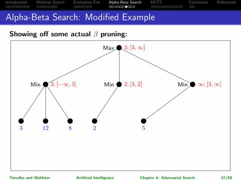
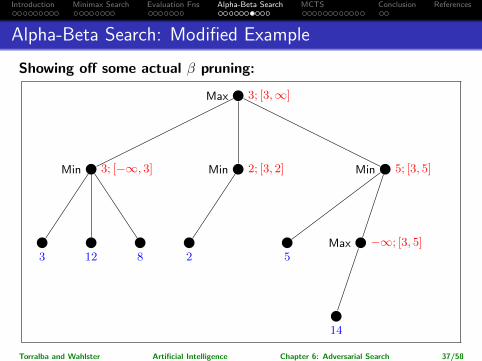
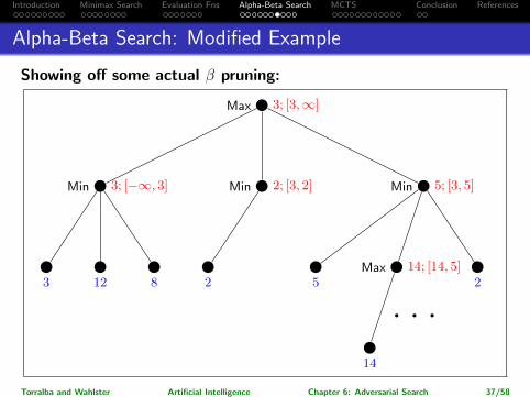
Alpha-Beta Search: Modified Example
Showing off some actual β pruning:
Max 3; [3,∞]
Min 3; [−∞, 3]
3 12 8
Min 2; [3, 2]
2
Min ∞; [3,∞]
Min 5; [3, 5]Min 2; [3, 2]
5
Max −∞; [3, 5]Max 14; [14, 5]
14
2
Torralba and Wahlster Artificial Intelligence Chapter 6: Adversarial Search 37/58
Introduction Minimax Search Evaluation Fns Alpha-Beta Search MCTS Conclusion References
Alpha-Beta Search: Modified Example
Showing off some actual β pruning:
Max 3; [3,∞]
Min 3; [−∞, 3]
3 12 8
Min 2; [3, 2]
2
Min ∞; [3,∞]
Min 5; [3, 5]
Min 2; [3, 2]
5Max −∞; [3, 5]
Max 14; [14, 5]
14
2
Torralba and Wahlster Artificial Intelligence Chapter 6: Adversarial Search 37/58
Introduction Minimax Search Evaluation Fns Alpha-Beta Search MCTS Conclusion References
Alpha-Beta Search: Modified Example
Showing off some actual β pruning:
Max 3; [3,∞]
Min 3; [−∞, 3]
3 12 8
Min 2; [3, 2]
2
Min ∞; [3,∞]
Min 5; [3, 5]
Min 2; [3, 2]
5
Max −∞; [3, 5]
Max 14; [14, 5]
14
2
Torralba and Wahlster Artificial Intelligence Chapter 6: Adversarial Search 37/58

Introduction Minimax Search Evaluation Fns Alpha-Beta Search MCTS Conclusion References
Alpha-Beta Search: Modified Example
Showing off some actual β pruning:
Max 3; [3,∞]
Min 3; [−∞, 3]
3 12 8
Min 2; [3, 2]
2
Min ∞; [3,∞]Min 5; [3, 5]
Min 2; [3, 2]
5
Max −∞; [3, 5]
Max 14; [14, 5]
14
2
Torralba and Wahlster Artificial Intelligence Chapter 6: Adversarial Search 37/58
Introduction Minimax Search Evaluation Fns Alpha-Beta Search MCTS Conclusion References
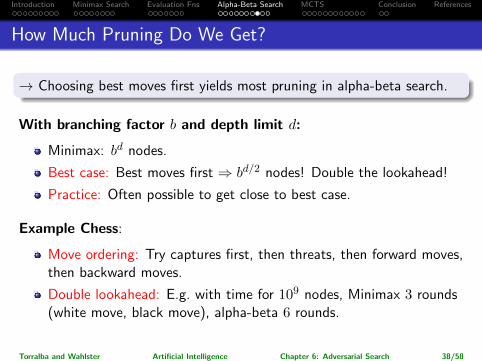
How Much Pruning Do We Get?
→ Choosing best moves first yields most pruning in alpha-beta search.
With branching factor b and depth limit d:
Minimax: bd nodes.
Best case: Best moves first ⇒ bd/2 nodes! Double the lookahead!
Practice: Often possible to get close to best case.
Example Chess:
Move ordering: Try captures first, then threats, then forward moves,then backward moves.
Double lookahead: E.g. with time for 109 nodes, Minimax 3 rounds(white move, black move), alpha-beta 6 rounds.
Torralba and Wahlster Artificial Intelligence Chapter 6: Adversarial Search 38/58

Introduction Minimax Search Evaluation Fns Alpha-Beta Search MCTS Conclusion References
Computer Chess State of the Art
Alpha-beta search.
Fast evaluation functions fine-tuned by human experts and training.
Case-based reasoning (positions from 2 million known games, in1997).
Very large game opening databases.
Very large game termination databases.
Fast hardware.
→ A mixture of (a) very fast search, and (b) human expertise.
→ Typically similar in other games (e.g. Checkers/Dame).
Except: Go!
Torralba and Wahlster Artificial Intelligence Chapter 6: Adversarial Search 39/58
Introduction Minimax Search Evaluation Fns Alpha-Beta Search MCTS Conclusion References
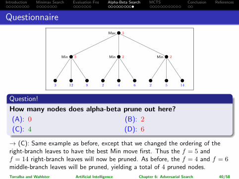
Questionnaire
Max 3
Min 3
3 12 8
Min 2
2 4 6
Min 2
2 5 14
Question!
How many nodes does alpha-beta prune out here?
(A): 0
(C): 4
(B): 2
(D): 6
→ (C): Same example as before, except that we changed the ordering of theright-branch leaves to have the best Min move first. Thus the f = 5 andf = 14 right-branch leaves will now be pruned. As before, the f = 4 and f = 6middle-branch leaves will be pruned, yielding a total of 4 pruned nodes.
Torralba and Wahlster Artificial Intelligence Chapter 6: Adversarial Search 40/58

Introduction Minimax Search Evaluation Fns Alpha-Beta Search MCTS Conclusion References
And now . . .
AlphaGo = Monte-Carlo tree search + neural networks
Torralba and Wahlster Artificial Intelligence Chapter 6: Adversarial Search 42/58
Introduction Minimax Search Evaluation Fns Alpha-Beta Search MCTS Conclusion References
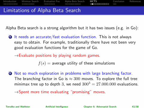
Limitations of Alpha Beta Search
Alpha Beta search is a strong algorithm but it has two issues (e.g. in Go):
1 It needs an accurate/fast evaluation function. This is not alwayseasy to obtain. For example, traditionally there have not been verygood evaluation functions for the game of Go.
→Evaluate positions by playing random games.
f(s) = average utility of these simulations
2 Not so much exploration in problems with large branching factor.The branching factor in Go is ≈ 300 moves. To explore the full treeminimax tree up to depth 3, we need 3003 = 27.000.000 evaluations.
→Spent more time evaluating “promising” moves.
Torralba and Wahlster Artificial Intelligence Chapter 6: Adversarial Search 43/58
Introduction Minimax Search Evaluation Fns Alpha-Beta Search MCTS Conclusion References
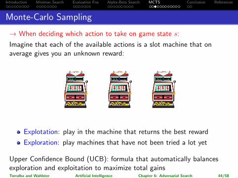
Monte-Carlo Sampling
→ When deciding which action to take on game state s:
Imagine that each of the available actions is a slot machine that onaverage gives you an unknown reward:
Explotation: play in the machine that returns the best reward
Exploration: play machines that have not been tried a lot yet
Upper Confidence Bound (UCB): formula that automatically balancesexploration and exploitation to maximize total gainsTorralba and Wahlster Artificial Intelligence Chapter 6: Adversarial Search 44/58

Introduction Minimax Search Evaluation Fns Alpha-Beta Search MCTS Conclusion References
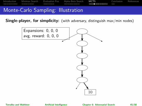
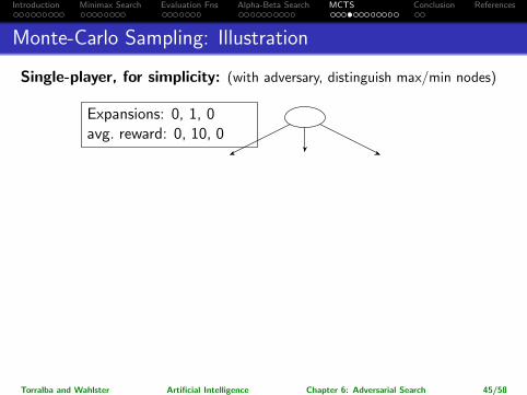
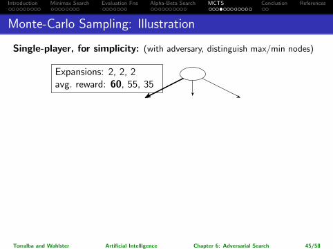
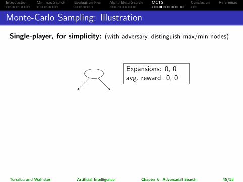
Monte-Carlo Sampling: Illustration
Single-player, for simplicity: (with adversary, distinguish max/min nodes)
40
70 50 30
100 10
Expansions: 0, 0, 0avg. reward: 0, 0, 0
Expansions: 0, 0avg. reward: 0, 0
Torralba and Wahlster Artificial Intelligence Chapter 6: Adversarial Search 45/58
Introduction Minimax Search Evaluation Fns Alpha-Beta Search MCTS Conclusion References
Monte-Carlo Sampling: Illustration
Single-player, for simplicity: (with adversary, distinguish max/min nodes)
40
70 50 30
100
10
Expansions: 0, 0, 0avg. reward: 0, 0, 0
Expansions: 0, 0avg. reward: 0, 0
Torralba and Wahlster Artificial Intelligence Chapter 6: Adversarial Search 45/58
Introduction Minimax Search Evaluation Fns Alpha-Beta Search MCTS Conclusion References
Monte-Carlo Sampling: Illustration
Single-player, for simplicity: (with adversary, distinguish max/min nodes)
40
70 50 30
100 10
Expansions: 0, 1, 0avg. reward: 0, 10, 0
Expansions: 0, 0avg. reward: 0, 0
Torralba and Wahlster Artificial Intelligence Chapter 6: Adversarial Search 45/58
Introduction Minimax Search Evaluation Fns Alpha-Beta Search MCTS Conclusion References
Monte-Carlo Sampling: Illustration
Single-player, for simplicity: (with adversary, distinguish max/min nodes)
40
70 50 30
100 10
Expansions: 2, 2, 2avg. reward: 60, 55, 35
Expansions: 0, 0avg. reward: 0, 0
Torralba and Wahlster Artificial Intelligence Chapter 6: Adversarial Search 45/58
Introduction Minimax Search Evaluation Fns Alpha-Beta Search MCTS Conclusion References
Monte-Carlo Sampling: Illustration
Single-player, for simplicity: (with adversary, distinguish max/min nodes)
40
70 50 30
100 10
Expansions: 0, 0avg. reward: 0, 0
Torralba and Wahlster Artificial Intelligence Chapter 6: Adversarial Search 45/58
Introduction Minimax Search Evaluation Fns Alpha-Beta Search MCTS Conclusion References
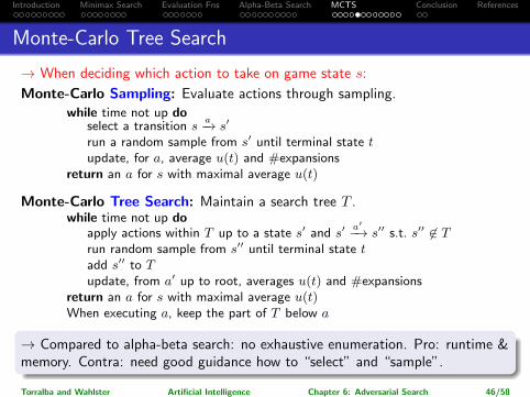
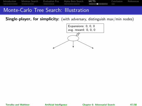
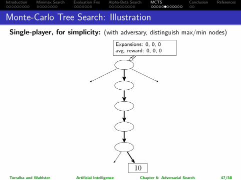
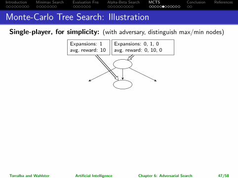
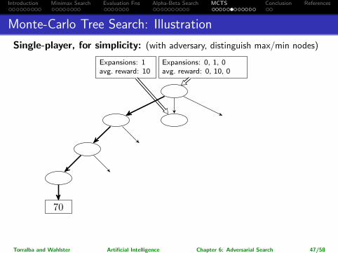
Monte-Carlo Tree Search
→ When deciding which action to take on game state s:
Monte-Carlo Sampling: Evaluate actions through sampling.
while time not up doselect a transition s
a−→ s′
run a random sample from s′ until terminal state tupdate, for a, average u(t) and #expansions
return an a for s with maximal average u(t)
Monte-Carlo Tree Search: Maintain a search tree T .while time not up do
apply actions within T up to a state s′ and s′a′−→ s′′ s.t. s′′ 6∈ T
run random sample from s′′ until terminal state tadd s′′ to Tupdate, from a′ up to root, averages u(t) and #expansions
return an a for s with maximal average u(t)When executing a, keep the part of T below a
→ Compared to alpha-beta search: no exhaustive enumeration. Pro: runtime &memory. Contra: need good guidance how to “select” and “sample”.
Torralba and Wahlster Artificial Intelligence Chapter 6: Adversarial Search 46/58
Introduction Minimax Search Evaluation Fns Alpha-Beta Search MCTS Conclusion References
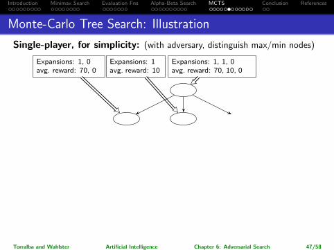
Monte-Carlo Tree Search: Illustration
Single-player, for simplicity: (with adversary, distinguish max/min nodes)
40
70 50 30
100 10
Expansions: 0, 0, 0avg. reward: 0, 0, 0
Torralba and Wahlster Artificial Intelligence Chapter 6: Adversarial Search 47/58
Introduction Minimax Search Evaluation Fns Alpha-Beta Search MCTS Conclusion References
Monte-Carlo Tree Search: Illustration
Single-player, for simplicity: (with adversary, distinguish max/min nodes)
40
70 50 30
100
10
Expansions: 0, 0, 0avg. reward: 0, 0, 0
Torralba and Wahlster Artificial Intelligence Chapter 6: Adversarial Search 47/58
Introduction Minimax Search Evaluation Fns Alpha-Beta Search MCTS Conclusion References
Monte-Carlo Tree Search: Illustration
Single-player, for simplicity: (with adversary, distinguish max/min nodes)
40
70 50 30
100 10
Expansions: 0, 1, 0avg. reward: 0, 10, 0
Expansions: 1avg. reward: 10
Torralba and Wahlster Artificial Intelligence Chapter 6: Adversarial Search 47/58
Introduction Minimax Search Evaluation Fns Alpha-Beta Search MCTS Conclusion References
Monte-Carlo Tree Search: Illustration
Single-player, for simplicity: (with adversary, distinguish max/min nodes)
40
70
50 30
100 10
Expansions: 0, 1, 0avg. reward: 0, 10, 0
Expansions: 1avg. reward: 10
Torralba and Wahlster Artificial Intelligence Chapter 6: Adversarial Search 47/58
Introduction Minimax Search Evaluation Fns Alpha-Beta Search MCTS Conclusion References
Monte-Carlo Tree Search: Illustration
Single-player, for simplicity: (with adversary, distinguish max/min nodes)
40
70 50 30
100 10
Expansions: 1, 1, 0avg. reward: 70, 10, 0
Expansions: 1, 0avg. reward: 70, 0
Expansions: 1avg. reward: 10
Torralba and Wahlster Artificial Intelligence Chapter 6: Adversarial Search 47/58

Introduction Minimax Search Evaluation Fns Alpha-Beta Search MCTS Conclusion References
Monte-Carlo Tree Search: Illustration
Single-player, for simplicity: (with adversary, distinguish max/min nodes)
40
70 50 30
100 10
Expansions: 2, 2, 2avg. reward: 60, 55, 35
Expansions: 2, 0avg. reward: 60, 0
Expansions: 2avg. reward: 55
Expansions: 2, 0avg. reward: 35, 0
Expansions: 0, 1avg. reward: 0, 50
Expansions: 1avg. reward: 100
Expansions: 0, 1avg. reward: 0, 30
Torralba and Wahlster Artificial Intelligence Chapter 6: Adversarial Search 47/58
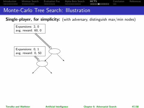
Introduction Minimax Search Evaluation Fns Alpha-Beta Search MCTS Conclusion References
Monte-Carlo Tree Search: Illustration
Single-player, for simplicity: (with adversary, distinguish max/min nodes)
40
70 50 30
100 10
Expansions: 2, 0avg. reward: 60, 0
Expansions: 0, 1avg. reward: 0, 50
Torralba and Wahlster Artificial Intelligence Chapter 6: Adversarial Search 47/58
Introduction Minimax Search Evaluation Fns Alpha-Beta Search MCTS Conclusion References
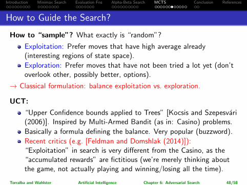
How to Guide the Search?
How to “sample”? What exactly is “random”?
Exploitation: Prefer moves that have high average already(interesting regions of state space).
Exploration: Prefer moves that have not been tried a lot yet (don’toverlook other, possibly better, options).
→ Classical formulation: balance exploitation vs. exploration.
UCT:
“Upper Confidence bounds applied to Trees” [Kocsis and Szepesvari(2006)]. Inspired by Multi-Armed Bandit (as in: Casino) problems.
Basically a formula defining the balance. Very popular (buzzword).
Recent critics (e.g. [Feldman and Domshlak (2014)]):“Exploitation” in search is very different from the Casino, as the“accumulated rewards” are fictitious (we’re merely thinking aboutthe game, not actually playing and winning/losing all the time).
Torralba and Wahlster Artificial Intelligence Chapter 6: Adversarial Search 48/58
Introduction Minimax Search Evaluation Fns Alpha-Beta Search MCTS Conclusion References
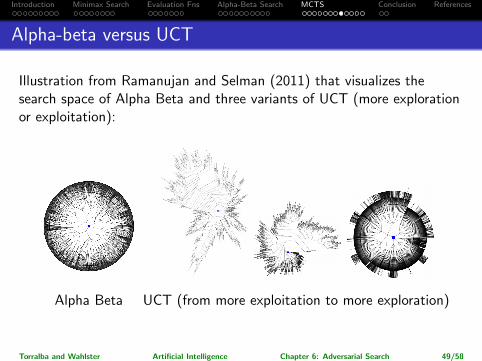
Alpha-beta versus UCT
Illustration from Ramanujan and Selman (2011) that visualizes thesearch space of Alpha Beta and three variants of UCT (more explorationor exploitation):
Alpha Beta UCT (from more exploitation to more exploration)
Torralba and Wahlster Artificial Intelligence Chapter 6: Adversarial Search 49/58
Introduction Minimax Search Evaluation Fns Alpha-Beta Search MCTS Conclusion References
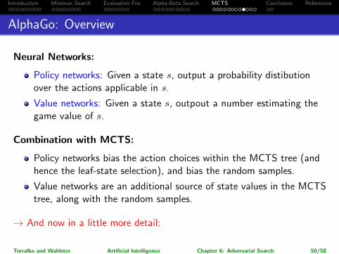
AlphaGo: Overview
Neural Networks:
Policy networks: Given a state s, output a probability distibutionover the actions applicable in s.
Value networks: Given a state s, outpout a number estimating thegame value of s.
Combination with MCTS:
Policy networks bias the action choices within the MCTS tree (andhence the leaf-state selection), and bias the random samples.
Value networks are an additional source of state values in the MCTStree, along with the random samples.
→ And now in a little more detail:
Torralba and Wahlster Artificial Intelligence Chapter 6: Adversarial Search 50/58

Introduction Minimax Search Evaluation Fns Alpha-Beta Search MCTS Conclusion References
Neural Networks
Input layer: Description of the game stateOutput layer: What we want to predict (e.g. utility of the state invalue networks, probability of a in policy networks)Supervised Learning: Given a set of training data (positions forwhich we know their utility), configure the net so that the error isminimized for those positions.
Torralba and Wahlster Artificial Intelligence Chapter 6: Adversarial Search 51/58
Introduction Minimax Search Evaluation Fns Alpha-Beta Search MCTS Conclusion References
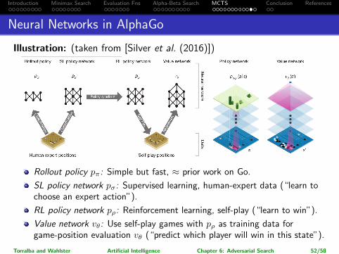
Neural Networks in AlphaGo
Illustration: (taken from [Silver et al. (2016)])
Rollout policy pπ: Simple but fast, ≈ prior work on Go.
SL policy network pσ: Supervised learning, human-expert data (“learn tochoose an expert action”).
RL policy network pρ: Reinforcement learning, self-play (“learn to win”).
Value network vθ: Use self-play games with pρ as training data forgame-position evaluation vθ (“predict which player will win in this state”).
Torralba and Wahlster Artificial Intelligence Chapter 6: Adversarial Search 52/58
Introduction Minimax Search Evaluation Fns Alpha-Beta Search MCTS Conclusion References
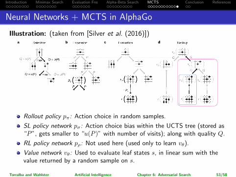
Neural Networks + MCTS in AlphaGo
Illustration: (taken from [Silver et al. (2016)])
Rollout policy pπ: Action choice in random samples.
SL policy network pσ: Action choice bias within the UCTS tree (stored as“P”, gets smaller to “u(P )” with number of visits); along with quality Q.
RL policy network pρ: Not used here (used only to learn vθ).
Value network vθ: Used to evaluate leaf states s, in linear sum with thevalue returned by a random sample on s.
Torralba and Wahlster Artificial Intelligence Chapter 6: Adversarial Search 53/58
Introduction Minimax Search Evaluation Fns Alpha-Beta Search MCTS Conclusion References
Summary
Games (2-player turn-taking zero-sum discrete and finite games) can beunderstood as a simple extension of classical search problems.
Each player tries to reach a terminal state with the best possible utility(maximal vs. minimal).
Minimax searches the game depth-first, max’ing and min’ing at therespective turns of each player. It yields perfect play, but takes time O(bd)where b is the branching factor and d the search depth.
Except in trivial games (Tic-Tac-Toe), Minimax needs a depth limit andapply an evaluation function to estimate the value of the cut-off states.
Alpha-beta search remembers the best values achieved for each playerelsewhere in the tree already, and prunes out sub-trees that won’t bereached in the game.
Monte-Carlo tree search (MCTS) samples game branches, and averagesthe findings. AlphaGo controls this using neural networks: evaluationfunction (“value network”), and action filter (“policy network”).
Torralba and Wahlster Artificial Intelligence Chapter 6: Adversarial Search 55/58
Introduction Minimax Search Evaluation Fns Alpha-Beta Search MCTS Conclusion References
Reading
Chapter 5: Adversarial Search, Sections 5.1 – 5.4 [Russell andNorvig (2010)].
Content: Section 5.1 corresponds to my “Introduction”, Section 5.2corresponds to my “Minimax Search”, Section 5.3 corresponds tomy “Alpha-Beta Search”. I have tried to add some additionalclarifying illustrations. RN gives many complementary explanations,nice as additional background reading.
Section 5.4 corresponds to my “Evaluation Functions”, but discussesadditional aspects relating to narrowing the search and look-up fromopening/termination databases. Nice as additional backgroundreading.
I suppose a discussion of MCTS and AlphaGo will be added to thenext edition . . .
Torralba and Wahlster Artificial Intelligence Chapter 6: Adversarial Search 56/58
Introduction Minimax Search Evaluation Fns Alpha-Beta Search MCTS Conclusion References
References I
Zohar Feldman and Carmel Domshlak. Simple regret optimization in online planningfor markov decision processes. Journal of Artificial Intelligence Research,51:165–205, 2014.
Levente Kocsis and Csaba Szepesvari. Bandit based Monte-Carlo planning. InJohannes Furnkranz, Tobias Scheffer, and Myra Spiliopoulou, editors, Proceedingsof the 17th European Conference on Machine Learning (ECML 2006), volume 4212of Lecture Notes in Computer Science, pages 282–293. Springer-Verlag, 2006.
Raghuram Ramanujan and Bart Selman. Trade-offs in sampling-based adversarialplanning. In Fahiem Bacchus, Carmel Domshlak, Stefan Edelkamp, and MalteHelmert, editors, Proceedings of the 21st International Conference on AutomatedPlanning and Scheduling (ICAPS’11). AAAI Press, 2011.
Stuart Russell and Peter Norvig. Artificial Intelligence: A Modern Approach (ThirdEdition). Prentice-Hall, Englewood Cliffs, NJ, 2010.
Torralba and Wahlster Artificial Intelligence Chapter 6: Adversarial Search 57/58
Introduction Minimax Search Evaluation Fns Alpha-Beta Search MCTS Conclusion References
References II
David Silver, Aja Huang, Christopher J. Maddison, Arthur Guez, Laurent Sifre, Georgevan den Driessche, Julian Schrittwieser, Ioannis Antonoglou, Veda Panneershelvam,Marc Lanctot, Sander Dieleman, Dominik Grewe, John Nham, Nal Kalchbrenner,Ilya Sutskever, Timothy Lillicrap, Madeleine Leach, Koray Kavukcuoglu, ThoreGraepel, and Demis Hassabis. Mastering the game of Go with deep neural networksand tree search. Nature, 529:484–503, 2016.
Torralba and Wahlster Artificial Intelligence Chapter 6: Adversarial Search 58/58