HAL Id: hal-01353399https://hal.archives-ouvertes.fr/hal-01353399

Submitted on 11 Aug 2016

HAL is a multi-disciplinary open accessarchive for the deposit and dissemination of sci-entific research documents, whether they are pub-lished or not. The documents may come fromteaching and research institutions in France orabroad, or from public or private research centers.

L’archive ouverte pluridisciplinaire HAL, estdestinée au dépôt et à la diffusion de documentsscientifiques de niveau recherche, publiés ou non,émanant des établissements d’enseignement et derecherche français ou étrangers, des laboratoirespublics ou privés.

Art of Modeling in Contact MechanicsMichel Raous

To cite this version:Michel Raous. Art of Modeling in Contact Mechanics. Friedrich Pfeiffer, Hartmut Bremer. The Artof Modeling Mechanical Systems, 570, Springer, 2016, CISM courses and Lectures, 9783319402550.hal-01353399

Art of Modeling in Contact Mechanics

Michel Raous

Aix-Marseille Univ, CNRS, Centrale Marseille, LMA, Franceraous@lma.cnrs-mrs.fr ∗

Abstract In this chapter, we will first address general issues of theart and craft of modeling - contents, concepts, methodology. Then,we will focus on modeling in contact mechanics, which will give theopportunity to discuss these issues in connection with non-smoothproblems. It will be shown that the non-smooth character of thecontact laws raises difficulties and specificities at every step of themodeling process. A wide overview will be given on the art of mod-eling in contact mechanics under its various aspects: contact laws,their mechanical basics, various scales, underlying concepts, math-ematical analysis, solvers, identification of the constitutive param-eters and validation of the models. Every point will be illustratedby one or several examples.

1 Modeling: the bases

It would be ambitious to try to give a general definition of the concepteither of a model itself or of model processing. Modeling relates to thegeneral process of production of scientific knowledge and also to the scientificmethod itself. It could be deductive (from the general to the particular, asprivileged by Aristotle) or inductive (making sense of a corpus of raw data).Descartes (38) saw in the scientific method an approach to be followed stepby step to get to a truth. Modeling can be effectively regarded as a scientificmethod that proceeds step by step, but its objective is more modest: to givesense of an observation or an experiment, and above all to predict behaviorswithin the context of specific assumptions. This concept of ”proceeding stepby step” is fundamental in modeling.

In this first section, we will examine the notion of model in the generalcontext of mechanical systems. The main features of these models are their

∗

The author is grateful to Prof. Marius Cocou for his very constructive comments on

the mathematical aspects and Prof. Alfredo Soldati for our very interesting discussion

on the general topic.

1

contents, their purposes, the way to build them, the way to use them, theexpectations and challenges.

Some of the reflections presented in this section find inspiration in thebook entitled Mathematical Modeling Techniques written by Aris Ruther-ford, from University of Caltech, in the 80s (108).

1.1 The objectives

The objective of modeling is twofold: explaining and understanding, giv-ing sense to experimental observations on the one hand, predicting behaviorson the other one.

Understanding.The models we are talking about all start from experimental observationsto which we want to give sense (deductive approach) and that we wish toexplain, understand and describe using the basic laws of mechanics andadding ”properly” chosen theoretical ingredients. The term ”properly” isfundamental and could be very constraining.

With the goal of understanding, the approach consists in gathering theinherent elements based on concepts necessary to build the systems of equa-tions to be solved. Behind that, there are some questions that should beanswered: do the solutions exist, are these solutions unique, are they sta-ble, are there methods (existing or to be developed) for solving them? Inother words, a model is part of a theoretical mechanical and mathematicalframework, and it will be essential to make sure that this framework hasbeen properly chosen, that there is consistency between the equations andthe framework, and that the possible limitations can be identified.

The main ingredients when building models in Mechanics are based onthe fundamental laws of mechanics and thermodynamics, as well as on thoseof physics, electricity and chemistry, and they need either the use or thedevelopment of mathematical tools. In the following we will present how, insome cases, modeling requires new mathematical developments, this beingparticularly true for contact problems. The problems studied today areincreasingly complex, due to interactions between phenomena of differentnatures, and multiphysic models can be considered.

Using or developing ingredients that have a meaning with respect to someconcepts to construct a scientifically coherent model is an essential featureof the art of modeling. This refers to the objectives of ”understanding” and”giving sense” in modeling.

Before going any further into the analysis of the modeling processes, letus make mention of other types of approaches. The notion of modeling thatwe present in the following is actually restrictive, and there are branches of

2

the modeling that differ markedly in their concept. Let us present two ofthem.

Note 1. When we associate modeling to ”equations”, we cut off otherapproaches which are directly based on experiments without theoreticallink or at least without a formal theoretical link. Let us give an example ofexperience-based modeling by referring to the work of the Catalan architectGaudi, known, among others things, for the basilica church ”La SagradaFamilia” in Barcelona. For the design of its arches, Gaudi developed thereversed chain model. He created mockups, using chains simulating thearches weighted with small bags to simulate the bearing forces applied bythe supporting pillar on the arch. Then, a mirror placed below gave thereversed image of the structure and showed the final shape of the real archdesign (see Fig. 1). He also used small hanging bags (full of salt or flour)for the representation of the shapes and the volumes of the domes, thecupolas, the arches and the pillars. The modeling process uses directlymeasurements of the mechanical behavior of the mockup without settinga theoretical framework as we will do in the following. However Gaudi’sarchitectural pieces of art brilliantly illustrate the efficiency of the reversedhanging chain model and of this kind of modeling approach.

Figure 1. Reversed chain model and cathedral church La Sagrada Familia

Note 2. Another class of modeling that we will overlook in this presen-tation is the one based on statistical considerations. In that case, from a(if possible large) number of experiments or random draws, we build a pre-dictive behavior or determine a solution to the problem using sophisticatedstatistical tools. The Monte Carlo methods have been the basis for this kindof approach. The Monte Carlo method was invented by Metropolis-Ulam

3

(73). This class of methods is based on random drawings chosen accordingto suitable probability distributions. Let us give an example. The acousticfield radiated by a source in a volume of any shape may be determinedwithout solving the wave equation but by using a ray theory: the acousticfield is then evaluated as the superposition of the trajectories of sound shotsfired from the source in random directions, the absorption by the walls beingtaken into account in the reflection rule. This approach works quite well aslong as the edge diffraction phenomena are not too important. Of course,the higher the number of shots is, the better the approximation is.

Examples of various methods employing statistical and probability toolsin the modeling process itself include variance reduction, polynomial chaos,kriging (used in geostatistics, meteorology, environmental sciences and elec-tromagnetism), as well as fractal analysis (see Cherepanov-Balakin (18)).The latter, more recent, is widely used in many fields. Among them can becited characterization and analysis of rough surfaces, dynamic cracking andelasticity of polymers or rubbers (18), analysis or monitoring of industrialprocesses, fault detection in machines, etc.

Predicting.Beyond providing the satisfaction of a better understanding, the main pur-pose of modeling is to predict, that is to say, replace experimentation bysimulation to predict the behavior of a mechanical system submitted to newloads, i.e., different from those used for building and validating the model.Replacing the experiment by a simulation via computation or analyticalanalysis is a crucial challenge, for two reasons at least. In the first place,replacing a time-consuming and costly experiment by some calculations willbe comfortable and economical (although it can also be very expensive attimes). Secondly, calculations are indispensable when experiments are notfeasible or very difficult to conduct, as in cases such as accidental eventsor natural disasters (a tsunami, the collapse of a dam or a pipe in an irra-diated environment, a nuclear explosion, the movement of a cyclone, etc.).Weather forecasting is a daily example of modeling. In some cases, experi-ments are performed using mockups but the scale effects remain a problemwhich should be considered with great caution.

It is to be understood that, for a reliable behavior prediction, the chal-lenges of modeling are the validation of the model, the study of its reliabilityand the identification of its domains of validity.

The objective ”understanding” is the basis for the objective ”predicting”,and it has an even more fundamental purpose. On the other hand, theeconomic stakes involved in ”predicting” are enormous: a validated modelwill drastically reduce the development period and the development cost for

4

a new product (in the broad sense of the term).Modeling is the alternative to a trial-error experimental process, which

consists in the construction of experimental protocols conducted by testingthe influence of the parameters considered as significant. This approach willbe possible for systems exhibiting a linear behavior (which of course willhave to be verified) but will soon become intractable in case of nonlinearbehaviors, due to the required number of experiments and given the timefor and the cost of making each specimen and conducting each experiment.Developing a good model will represent an important challenge.

A validated model will permit the optimization of a mechanical system.It will be an efficient tool in the hands of the engineer who will be able totest the influence of every parameter rapidly. A model is not a universaltool that would replace the scientist. It is only a sophisticated tool thatwill help the designer or the researcher during the process of creating oroptimizing a new product. Their skills in developing, selecting and usingthe models are indeed of central importance in the art of modeling.

Let us now get an overview on the various steps of the construction of amodel:

• the founding step is the choice of the equations chosen to describethe phenomenon which has to be modeled: some assumptions haveto be made, the main characteristics to take into account have to beidentified, the scale of the analysis has to be chosen, etc.,

• then comes the formulation step, with the choice of the formulationframework,

• the mathematical analysis of the problem should give informationabout the existence, uniqueness and stability of solutions, and moregenerally information about the conditioning of the problem to besolved,

• then comes the step of solving the problem which is obviously a keystep which leads to numerous developments and may give rise to verydifficult problems; this should be completed on the one hand by thenumerical analysis of the approximate problem, of the discrete prob-lem and of the algorithms and on the other hand by the validation ofthe numerical method,

• once the numerical tool is ready, the basic constitutive parameter haveto be identified using the model to simulate a test experiment; thesensitivity of the solutions to some changes of the parameter valuesshould also be tested,

• and finally the last step is the validation of the model by simulatingvarious experiments and evaluating the error between the theoreticaland the experimental results.

5

Some of these steps can be more or less important and more or less difficultdepending on the cases, but it will be important and useful to keep all ofthem in mind.

1.2 Construction of a model

The art of the modeler will be about highlighting the key points andidentifying the nature of the significant phenomena and their contributionsin various experiments. The basic step in building a model is the choice ofthe ingredients to use and of the assumptions to make. It will be essential tobear in mind that a model is composed of ”equations” and ”assumptions.”These underlying assumptions will be the bases of the validity domain ofthe model and they have to be clearly defined and remembered. This mayseem obvious but transgressions are common: for example, using numericalintegration methods based on limited developments for computing solutionsthat are not differentiable would be incorrect.

Concerning the assumptions, there are also some subtleties, such as thedifference between simplification and neglect. The former permits to solvethe problem but is not necessarily legitimate (and that should be studied)while the latter consists in neglecting a secondary aspect of the problem(and that is a justified assumption).

We can try to list and classify by nature some of these choices and as-sumptions that will be made during the construction of the model and of thesystems of equations to solve, in order to correctly simulate the experiment.

• The physics that should be taken into account. The first step is toidentify the nature of the significant phenomena which have to be con-sidered: mechanical, chemical, thermal, electrical effects or other ef-fects. This defines the degree of complexity of the model. Multiphysicmodeling is increasingly used today. This step is very important be-cause neglecting a significant effect (incomplete model) would haveas harmful effects as taking into account a side effect (unnecessarilycomplicated model).

• The ”equations” and their framework. The ”equations” will be writtenin the general framework of the fundamental principles of mechanicsand thermodynamics. Their implementation gives rise to differences inpoints of view, equations of motion or energy principles, partial differ-ential equations or minimum problems, etc. The degree of generalityor abstraction of the framework will define the degree of generalityof the model. We will speak of classes of models when this degree ofgenerality is great. This will be illustrated in Section 2.5 by a workwhere we introduce a unified model for adhesive interfaces based on

6

considerations such as the concept of generalized standard materialsextended to interfaces.

• The role of time. Time plays a special role in the development ofa model. Several questions arise and have to be answered. The firstquestion is whether a dynamic study should be conducted, if the effectsof inertia are to be taken into account, or a quasi-static approach issufficient, if masses are small enough or phenomena slow enough.

Another question concerns the possible influence of the velocitieson the nature of the behaviors and if viscous dissipation should beconsidered.

A third question is whether the effects of variations in time ofthe parameters should be taken into account, either directly (effect ofaging for example) or indirectly, these parameters depending on someof the variables such that displacements or velocities.

When the phenomenon depends on the loading path (plasticity,damage, etc.), then we are in a rather special case where time isreplaced by a dimensionless variable characterizing the loading path.

• Choice of the scale. Another specific issue when building a modelis the choice of the scale to conduct the analysis. It could be onlythe choice of a given scale or that of the combination of several scales(multiscale model). With the phenomenal increase in computer power,multi-scale approaches are experiencing spectacular growth.

1.3 Choosing a formulation

Choosing a formulation relates several levels. First, we can choose adiscrete or a continuous formulation. Secondly, it has to be noted that thechoice of the variables is directly connected to the form of the formulation(primal, dual or mixed formulation).

A discrete formulation consisting in assembling masses, springs and var-ious elements in general has as objective to ”understand”. A discrete for-mulation can be very sophisticated, including nonlinear or specific items.Such example is presented in Section 1.9. The target to ”simulate” and to”predict” the behavior of complex structures rather goes through continu-ous formulations associated with finite element methods which may workfor any geometry. But many variants are possible and the combination ofdiscrete and continuous formulations is often useful for complex assemblies.

The mathematical framework is closely relates to the formulation. Totake some examples in continuum mechanics, the general framework forsmooth problems will be that of functional analysis and Sobolev spaces.In some cases, such as contact problems discussed later the convenientframework will be the ones of convex and non-convex analysis. As for the

7

variational formulations, we will distinguish among primal (displacementor velocity formulation), dual (stress formulations) or mixed formulations,each having its own advantages and disadvantages depending on the situa-tion. In the case of non-smooth problems with respect to time, a convenientframework will be that of distributions and differential measures.

For non-smooth problems, the formulations and their mathematical frame-work may be drastically simplified by using regularizations. However, theseprocesses may create a problem markedly different from the initial problem,which can have an impact on the validity of the model. A special section inthe following will be devoted to that important issue.

1.4 The framework and the mathematical analysis

Although often considered as unnecessary or irrelevant, or else as anexercise for mathematicians, mathematical analysis has a leading role inthe art of modeling. For smooth problems (with respect to time as wellas space variables) the mathematical framework is very classical and doesnot need special care. However, it can be noted that only the writing ofboundary conditions for partial differential equations uses the concept oftrace in Sobolev spaces.

Note that whole areas of mathematics have been developed from prob-lems in mechanics: some aspects of functional analysis, convex analysis,the notion of Γ-convergence, etc. (see Dautray-Lions (33)). Mechanicalproblems, especially non-smooth problems, have promoted very high levelmathematical developments which are still ongoing. Unfortunately, despitegiving an adequate framework, they sometimes lead to results that cannotbe quantitatively used directly by engineers. However, they always help inthe understanding of both the model and the computational behaviors. Thetheoretical framework and the mathematical analysis are very constructivein setting the problems properly, understanding the main theoretical prop-erties and developing convenient numerical methods for the resolution. Wewant to stress that using the right mathematical context adapted to theingredients (equations) put into the model is a key point in the art of mod-eling, the only way to find and to characterize the right solutions, includingsometimes some unexpected ones.

We will illustrate that in the following. Contact mechanics will be a goodcontext to discuss modeling in these various aspects. Although the lawsseem very simple (Coulomb’s law dates back to the 18th century), everythingis very complicated because they relate to non-smooth mechanics: thresholdlaws, the graphs of the contact laws are multivalued mappings and notfunctions, etc.

8

1.5 Resolution

It is obviously a key step in the art of modeling. The resolution couldbe analytical: it is then limited to elementary geometries, but it simplifiesparametric studies and helps to identify the essential phenomena more eas-ily. More generally, analytical approaches are useful to ”understand” andhence they must not be neglected in modeling.

But today, the methods of resolution are mostly numerical and the greatincrease in computer power has paved the way not only for new methodsbut also for new ways of thinking about modeling approaches. There is nowin the art of modeling a close link between resources and computing powerand design patterns.

We would like to point out a downside risk associated with this increasingcomputational power. It is the risk of replacing ”thinking” by ”large numberof degrees of freedom”. This is undoubtedly one of the main common pitfallsof modeling. A lot of computations using millions of Degrees Of Freedom(DOF) will very often provide less on the knowledge and the understandingof a problem than a well thought out model using a small number of DOFsor a discrete mechanical model.

The range of existing methods is very wide and in constant development.Without trying to be exhaustive, one may mention the finite element meth-ods (FEM) and their variants ((FEM)2, subdomains, multigrid methods,diffuse elements, etc.), finite volume methods, integral methods, spectralmethods, etc.

It is worth stressing several points about numerical methods and com-putations.

First, it will be important to keep in mind that a numerical method mustbe consistent with the assumptions and with the mathematical framework.

Another extremely important point is the validation of the numericalmethod itself (see Section 4). This must be done using standard solutionsthat can be analytical or qualified by other methods (benchmarks). This isnot trivial matter and it is sometimes possible to find numerical methodsvalidated with an experiment - which is absurd. What is more, this step ofvalidation of the numerical method will generally be an opportunity to eval-uate and control the numerical errors (distinguishing between discretizationerrors and calculation errors), check convergence conditions, properly selectcalculation parameters, etc.

The numerical analysis of the approached problems and of the discreteproblems is often overlooked because it is often difficult. However, it willprovide important information about the stability of the algorithms (andpossibly provide the stability conditions to be verified), on convergence, er-

9

ror estimates and other properties that will be valuable during the numericalimplementation.

1.6 Identification of the parameters

The parameter identification step should be distinguished from the modelvalidation step - which we will be discussed in the following. This essen-tial step comes after the model construction step, and consists in finding asolution to the optimization problem: finding the parameter values whichminimize the gap (the error) between one experiment and the results givenby the model simulation.

Generally, the identification of constitutive parameters is conducted withexperiments that are either independent of the problem addressed or closelylinked to it. For example, when modeling the behavior of a structure, themechanical properties of the materials are usually determined with experi-ments on specimens, thus independently of the system studied.

On the contrary, in other cases, these characteristics depend so much onthe environment of the system in real situation that it becomes necessaryto use other processes. This will generally be the case for interface models,as we will see later.

1.7 Validation of the model

This is of course the key step in modeling since it will allow us to givereliable behavior predictions when using the model. Validation is part of themost important steps in modeling; it will define the quality of the model,specifies the validity domain and confirm its ability to be used by the de-signer. It is essential and requires special care (see Section 4).

Validation is carried out on one or more experiments by evaluating theerror between the results of the experiments and those of the simulations,using the values of the constitutive parameters obtained by the identificationprocess. Let us note in passing that the norm selected to evaluate this erroris of great importance since a norm L2 (squared error), which inherentlycarries an energy sense, will smooth the gaps, while a norm L∞ (sup norm)will measure the maximum deviation which can in some cases be the decisivedimensioning factor.

Note that the experimental conditions should verify the assumptionsmade initially for the construction of the model (load amplitudes, speed,etc.).

At this level, adjustments to the model will be performed by iterationsbetween the model prediction and the experimental results. Two approachesmay be followed: either improving the model if the gap between theory and

10

experiment is not small enough or checking whether it is possible to simplifythe model while keeping an appropriate gap value. The second approach isoften overlooked.

1.8 To conclude this introductory chapter

In this chapter, we have addressed many aspects of modeling. As acomplement, we would like to stress two key points in the art of modeling.

This first key point is: ”Make as simple as possible and as complex asnecessary, no more, no less!”.

We will illustrate this with the example of the famous work of PabloPicasso, ”Bulls” (Picasso, 1945) presented on Fig. 2. ’Bull’ is a suite ofeleven lithographs that have become a master class in how to develop anartwork from the academic to the abstract. In this series of images, Picassovisually dissects the image of a bull to discover its essential presence througha progressive analysis of its form. Each plate is a successive stage in aninvestigation to find the absolute ”spirit” of the beast. In this work, Picassoprogressively simplifies the shape of the bull and keeps the quintessence ofthe draw. In the final print of the series, Picasso reduces the bull to a simpleoutline which is so carefully considered through the progressive developmentof each image that it captures the absolute essence of the creature in asconcise an image as possible. A critic made that comment: ”He has endedup where he should have started! He had gone in successive stages throughall the other bulls. When you look at that line you cannot imagine how muchwork it involved. He had in mind to retrieve the bull’s constituent parts, hisdream bull - bred of pure lines - an elemental, disembodied, quintessentialbullishness”. The result is the Platonic idea of a bull. The reverse process

Figure 2. The process followed by Picasso in the eleven lithographs ”Bull, 1945”

to get back to the initial complete image of the bull is the gain of knowledge.This development of knowledge to obtain the ideal model from a reality isthe basis of the art of modeling. The process of Picasso is in fact exactlyour only hope to gain knowledge.

11

In the same state of mind, we may also cite Fernando Pessoa: ”Thoughtmust start from the irreducible”.

The art of modeling consists precisely in building the simplest model con-taining the key characteristics of the phenomena and permitting its suitableand validated simulation. Making the model as simple as possible and ascomplex as necessary is really fundamental in the art of modeling: makingit too simple would be insufficient and making it too complex would beuseless and costly.

A second key point in the art of modeling is: you should not fall intothe trap of habit. One of the pitfalls the modeler must avoid when facedwith a new problem is the temptation to do ”what he does best ”ratherthan ”what he should do”, i.e., fitting the problem within the framework ofhis own mechanical engineering culture, of his usual tools (even followingnecessary new developments) instead of using a totally different approach,which should be more convenient, but not familiar to him. It is not easyto resist a natural temptation and it is thus often difficult to avoid thetrap of habit, as it requires a sound knowledge of models and modeling,when models are becoming increasingly sophisticated, and it is difficult tobe an all-rounder. It will be more constructive to work within multiple skillgroups or to liaise with a network of specialists, while having developed asufficiently broad knowledge, from experimentation to numerical methodsand mathematics, to be able to dialogue with those specialists. This varietyof knowledge in modeling is well known to industrialists, who sometimespresent the same problem to several academic research laboratories thatdiffer in their approaches.

To conclude on this chapter, we can say that, besides the broad spectrumof his scientific qualities, his in-depth knowledge, the thoroughness of hisanalysis, intuition will be a key asset for the modeler.

We will now illustrate some features of this section with an example frommechanics of materials, the cyclic behavior of a polyurethane foam, beforegetting to the art of modeling in contact mechanics in the next sections.

1.9 Step by step construction of a discrete model - Example ofthe modeling of the cyclic behavior of a polymeric foam

This problem, studied in the PhD thesis of Giampiero Pampolini ((82)(81) (36)), will be used to illustrate three points discussed in this section.

• ”Discrete model and analogical models” (springs, dashpots, etc.) helpto ”understand” and to identify the driving phenomena. We use a dis-crete model composed by assembling non-linear springs, dashpots andother convenient elements. The goal is not to simulate the behavior of

12

a whole structure but to identify and to model the main phenomenaoccurring in this kind of material during cyclic loadings.

• ”From simplicity to complexity”: the model is developed step by step.This second point relates to the idea to put into a model what isnecessary, no more, no less. We start with simple elements and weprogressively add other necessary elements.

• ”Identification of the constitutive parameters” and ”validation of themodel” which have to be clearly distinguished

This is a discrete model used to ”understand” and which is ”as simple aspossible and as complicated as necessary”. All details can be found in DelPiero-Pampolini-Raous (82) (81) (36).

Main characteristics of the behavior: the experiments.When a sample of an open-cell polymeric foam is submitted to quasi staticcompression, localization of the deformation can be observed with the oc-currence of bands orthogonal to the loading direction (see Fig. 3).

Figure 3. Localization of deformation during compression

0 0.2 0.4 0.6 0.80

2

4

6

8

10(a)

Deformation

Str

ess

(kP

a)

0 0.2 0.4 0.6 0.80

2

4

6

8

10(b)

Deformation

Str

ess

(kP

a)

0 0.2 0.4 0.6 0.80

2

4

6

8

10(c)

Deformation

Str

ess

(kP

a)

0 0.2 0.4 0.6 0.80

2

4

6

8

10(d)

Deformation

Str

ess

(kP

a)

Figure 4. Recovering (a) Virgin mate-rial, Resting period : (b) 16 hours ; (c)52 hours ; (d) 33 days.

0 0.2 0.4 0.6 0.80

2

4

6

8

10(a)

Deformation

Str

ess

(kP

a)

0 0.2 0.4 0.6 0.80

2

4

6

8

10(b)

Deformation

Str

ess

(kP

a)

0 0.2 0.4 0.6 0.80

2

4

6

8

10(c)

Deformation

Str

ess

(kP

a)

0 0.2 0.4 0.6 0.80

2

4

6

8

10(d)

Deformation

Str

ess

(kP

a)

Figure 5. Loading velocity influence:(a) 0.1 mm/min ; (b) 5 mm/min ; (c)100 mm/min ; (d) Comparison of the 3results.

13

When a cyclic compression is applied, the following characteristics of thestress/strain cycles are noted (see Fig. 4 and Fig. 5):

• specific shape of the cycles,• first cycle different from the next ones,• influence of the loading velocity,• influence of the resting periods on the behavior,• analogy with Mullins effect for elastomers (strain softening).

Discrete problem and nonlinear elasticity.A discrete model, an assembly of springs, dashpots and other convenientelements, is considered. The specimen will be considered as discretized intoa finite number of layers (Fig. 6). The art of modeling will consist inchoosing the good characteristics of the various constitutive elements of thechains. We will first address the localization phenomenon observed duringcompression. For that, we consider that the springs exhibit a nonlinearelasticity based on the non-convex strain energy density w presented in Fig.6 (details can be found in (81) (36)). Details on the analysis and on thecomputation of the response can be found in (82). The existence of twophases is characterized: one phase corresponding to the virgin cells and theother corresponding to the totally squeezed cells.

Figure 6. Representation of the cell lyers (a) by a chain of springs (b) with anon convex strain energy (c) which gives the behavior law (d) for each spring.

A good agreement is observed between the model and the experiment for thefirst compression step, but, either when unloading or when various loadingamplitudes are considered, there is a big gap between theory and experimentresults (even qualitatively), as shown in Fig. 7.

Viscosity effects are added.The model has to be completed by taking into account other phenomena.We will now introduce the viscosity effects. The idea is to incorporatewhat is necessary gradually into the model to describe the experimental

14

0 0.2 0.4 0.6 0.80

2

4

6

8

10

12

14(a)

Deformation

Str

ess

(kP

a)

0 0.2 0.4 0.6 0.80

2

4

6

8

10

12

14(b)

Deformation

Str

ess

(kP

a)

Figure 7. Comparison between the nonlinear elasticity model (a) and experiment(b) for different loading amplitudes.

behavior. We introduce a Zener model with Maxwell viscosity. This modelmay encounter both the loading rate dependence (classical viscosity effectduring the cycles) and a long period dependence (recovery of the initialproperties after resting periods which is a relaxation phenomenon). Forthat, we introduce several relaxation times with different time scales inthe viscosity model. In Fig. 8, it can be observed that a good agreementbetween theory (full line) and experiment (dotted line) is now obtainedregarding the shape of the cycles. Nevertheless, even if the first cycle isvery well described, it remains that the gap between the first cycle and thenext ones is not described.

0 0.1 0.2 0.3 0.4 0.5 0.6 0.70

2

4

6

8

10

Deformation

Str

ess

(kP

a)

Figure 8. Theory/experiment compar-ison when using the nonlinear elasticitymodel with viscosity

0 0.1 0.2 0.3 0.4 0.5 0.6 0.70

2

4

6

8

10(b)

Deformation

Str

ess (

kP

a)

Figure 9. Theory/experiment compar-ison when using nonlinear elasticity, vis-cosity and damage.

15

Damage is added.Once again, a new effect has to be taken into account and we introducedamage in the model. Now, as shown in Fig. 9 a very good agreementis obtained between the model simulation (full line) and the experimentalresults (dotted line). The complete model has been constructed step by step,progressively adding new concepts that are necessary to get an accuratedescription of the behaviors observed during the experiments.

A model to ”understand” Let us note that this discrete model is veryhelpful to understand the behavior of polymeric foam. ”Understanding”was presented as the first goal in the art of modeling in Section 1. Weexplain that this cyclic behavior is due to nonlinear elasticity, viscosity anddamage. The model shows clearly the phase-change mechanism occurringin the polymeric foam during the loading, which gives the shape of thestress/strain curve. With a simulation conducted with a chain of 120 el-ements, the panel of colors (Fig. 10) gives the deformation levels in thecolumn (this is a one dimensional model) corresponding to the differentpoints on the stress/strain curve: A, D, E and G are single phase configura-tions, while B, C, F and H are two phase configurations (in B, C and F thetwo phases are block separate). The points C, E and H show situations withdifferent stresses for the same deformation. This is due to the dependence ofthe solution on the loading path. A good understanding of the phenomenonis achieved.

0 0.1 0.2 0.3 0.4 0.5 0.6 0.70

1

2

3

4

5

6

7

8

9

10

Deformation

Str

ess (

kP

a)

A

BC

D

E

F

G

H

Figure 10. Evolution of the deformation condition (phase changes) during acycle (the color scale for the deformations is given on the far left)

How to validate the model ?The good theory-experiment agreement shown in Fig. 9 is the result of theprocess of identification of the constitutive parameters. The identificationwas a quite difficult process and details of the methodology will be presented

16

in Section 4.4 and in Pampolini-Raous (82). At this point (construction ofthe model and identification of the parameters), we only showed that thereis at least one set of parameter values that permits to fit the model with oneexperiment. The model is not yet validated and not ready to be used for”prediction”, the other goal of the art of modeling. In order to validate themodel, we will use it, with the parameters evaluated during the identificationprocess, to simulate other kinds of loadings. This time, a good agreementbetween theoretical predictions and experimental results will confirm thevalidation of the model. This will be shown at Section 4.4.

1.10 Conclusions about the art of modeling for this first example

This discrete model has helped to understand what the main mechanicalphenomena involved in the cyclic behavior of polymeric foam are and, whatis more, has proposed some forms for the various ingredients that have tobe used:

• nonlinear elasticity with non-convex strain energy (a form is pro-posed),

• viscoelasticity with at least two time scales (cycle period and durationof the resting periods); a Zener-Maxwell model could be convenient,

• damage.

What is more, this work on this discrete model gives an order of magnitudeof the various constitutive parameters for the mechanical model.

Let us note that the model has been constructed step by step in orderto make ”as simple as possible but as complex as necessary”. The way toconduct ”identification and validation” will be presented at Section 4.4.

The next step would be now to develop a continuous formulation ofthe problem and to use finite element methods to simulate the behaviorof a polymeric foam structure in engineering systems, such as energy ab-sorbers, seat cushions, packaging materials and lightweight composite sand-wich structures, etc. That is not simple but the present model helps tounderstand what the main ingredients are that should be put into such amodel.

2 Building models in contact mechanics

We will now address the art of modeling in contact mechanics. As alreadymentioned, contact mechanics is a field of interest for discussing the art ofmodeling, since many of the issues addressed in the previous section willraise difficult questions.

17

In this section, we will focus on the step ”building the model” - whichis the most mechanical part. We give a panorama of various contact laws(unilateral contact, friction, adhesion, wear, etc.) and present the diversityof the applications in various fields. The different scales that can be usedare presented: we give some elements and references on multiscale analysiswhich is expanding strongly. We show how a model is built on the basis ofconcepts. We stress the advantages versus the dangers of regularization.

This is illustrated with two examples:

• a law coupling unilateral contact, friction and adhesion (the RCCMmodel) to illustrate the importance of concepts as the basis of a newcontact model (thermodynamic analysis) and the mathematical com-plications; this is applied to an engineering problem: how to improvethe resistance of a composite material to the crack propagation bycontrolling and optimizing the behavior of the fiber/matrix interface,

• a unified model coupling contact, friction and adhesion to illustratethe inductive/deductive process when one elaborates a model on thebasis of fundamental mechanics (generalized standard materials).

2.1 Basic interface models

Let us present a panorama of the main interface laws corresponding tothe main usual behaviors that we want to describe: non penetration intothe obstacle, friction, adhesion, healing adhesion, wear, etc. Details can befound in Raous (95) (103) (97) and Sauer (109).

Unilateral conditions.The basis is to write that the solid cannot penetrate into the obstacle sup-posed to be rigid. It can be generalized to the contact between two de-formable solids. Let us consider a rigid obstacle, the solid occupying adomain Ω, let ΓC the part of the boundary Γ initially in contact with theobstacle, uc the displacement (trace on ΓC of the displacement u definedon Ω), R the contact force and n the outward normal vector to ΓC . Us-ing the following partition between normal and tangential components, thenon-penetration condition is described by the following Signorini conditionswhich constitute a complementarity formulation. The graph of this behav-ior law is given in Fig.11. This is not a function but a multivalued mapping.It is here that difficulties begin!

uc = unn+ ut R = Rnn+Rt

18

un ≤ 0

Rn ≤ 0 (1)

unRn = 0

Rn

Un

Figure 11. Unilateral conditions : theSignorini conditions

Rt

Vt

Figure 12. Friction law: the Coulomblaw

Friction: Coulomb - Amontons friction law. (see (32))The basic law of friction is the Coulomb law (1821) which was developedon the basis of experimental observations with moderate amplitude forces.First, it is a law with a threshold, no movement occurs unless the tangentialforce reaches a certain threshold, secondly, this threshold is directly propor-tional to the normal force and thirdly, the movement occurs in the directionopposite to that of the applied tangential force. This is expressed by thefollowing law:

‖Rt‖ ≤ µ|Rn| (2)

if ‖Rt‖ < µ|Rn| then ut = 0 (3)

if ‖Rt‖ < µ|Rn| then ut = −λRt with λ ≥ 0 (4)

This law seems to be very simple; only one parameter, the friction coefficientµ, is involved. However, at the same time, it is very complicated becauseit is not a function but a multivalued mapping (see Fig. 12), as for theunilateral conditions. It will drastically increase the difficulties when writingthe mathematical formulations and developing the numerical methods. Weshould stress that this non smooth character is precisely the fundamentalrichness of this law; it will make it possible to model specific behaviors suchas occurrence of instabilities (squeal, stick-slip, etc.), existence of multiplesolutions, etc. Therefore, it will be important to conveniently deal with thisnon smooth character; we are in the context of non-smooth mechanics.

The configuration space is given by the Coulomb cone in the force space(see Fig. 13). When the representative point is inside the cone, no move-ment occurs, when it reaches the boundary, sliding occurs with the direction

19

Rn

Rt

- Vt

Figure 13. The Coulomb cone

of the tangential force (and not orthogonally to the boundary of the domain,as it is the case for example in classical plasticity). Thus, we should notethat there is no normality rule (the friction law is non-associated) and thiswill lead to extra difficulties for the formulation (no minimum principle, aswe will see in Section 3.3). As announced in Section 1.3, various formu-lations can be given and modeling consists in selecting one among them.Other formulations of the Coulomb law can be given. Let us here brieflygive some of them (details can be found in Moreau (76)):

• maximum dissipation principle

Rt ∈ C ∀St ∈ C (St −Rt)ut ≥ 0 (5)

where, in 2D C = [−µRn,+µRn]• subdifferential formulation

−ut ∈ ∂ICt(Rn)(Rt) (6)

where ∂ICt(Rn)(Rt) is the subdifferential of the indicator function ofCt(Rn) with Ct(Rn) = P such that |P | ≤ −µRn

• dual subdifferential formulation

Rt ∈ ∂φRn(−ut) (7)

with φRn(−ut) = µRn‖ut‖

Possible regularizations.The comments presented in this section are of great importance for the artof modeling. Regularization is a natural tendency when we have to dealwith a non-smooth problem. It allows us to replace the initial problem by

20

Rn

Un

Figure 14. Compliance or penaliza-tion of the Signorini problem

Rt

Vt

Figure 15. Regularizations for theCoulomb friction Hyperbolic tangent(dotted line), square root (dashed line),polynomial (solid line)

a much simpler one, which is also simpler to solve. We want to stress avery important point: a regularized problem is different from the initialproblem and could even model a very different mechanical phenomenon.The modeler should be very aware of that. Contact problems may illustratethat point very well.

For contact problems, regularization will consist in replacing the multi-valued mappings by functions in order to obtain a smooth (but non-linear)problem.

• Regularization of the unilateral conditions: compliance or penalizationof the contact laws. As shown in Fig. 14, the contact behavior isnow characterized by a (non-linear) function. When penetration intothe obstacle occurs, a strong force is introduced so as to push thedeformable solid out of the obstacle. A classical choice is the followingone, where (un)+ denotes the positive part of the normal displacementand Cn and mn are two prescribed regularization parameters:

−Rn = Cn(un)mn

+ (8)

This is very comfortable for the analysis and the resolution but let uslook at the mechanical behavior. It has to be noted that we alwayshave penetration into the obstacle with two consequences: one is abad determination of the contact forces (which now depend on thecompliance parameters) and the other one is a penetration into theobstacle that could be unrealistic.

The term compliance is used when dealing with the mechanicalmodel while the term penalization is used when solvers are involved.

21

Sometimes, in order to give a mechanical interpretation of this reg-ularization, it is said that the penalization of the unilateral contact(or the compliance laws) is associated with the squeeze of the asperity.Actually, when the squeeze of an asperity is computed (in large plasticdeformations, see Raous-Sage (94)), it turns out that the coefficientsCn and mn are huge and do not correspond necessarily to the suitablevalues usually chosen to make computations easy to do. Therefore, itcould be recommended either not to use regularization for the non-penetration conditions or - especially when a standard computationalcode is used - to check the penetration in order to control if its mag-nitude is admissible for the problem under consideration.

• Regularization of the Coulomb friction. In Fig 15, various functionsused to regularize the Coulomb friction law are presented. Again, theCoulomb multivalued mapping is replaced by functions (which arenon-linear) and this will make the problem a lot simpler.

But it should be stressed that the new mechanical problem is to-tally different from the initial one: sliding always occurs, except if theapplied tangential force is equal to zero! This means that with a verysmall force, you can get the refrigerator sliding across the kitchenif you wait for a sufficiently long period of time! Obviously, this iswrong!

Therefore, special attention has to be paid to the choice of the regularizationparameters relative to the time scale. Very often, when the values of theseparameters are chosen so as to give a good approximation of the Coulomblaw, the regularized problem remains a stiff problem, ill-conditioned from anumerical point of view. When the values of these parameters are chosenfor computational convenience, the quality of the solution has to be checkedwith respect to the Coulomb conditions, to be sure that this quality issufficient for the problem.

Otherwise, the choice of the regularization parameters has a great influ-ence on the tangential forces. Thus, let us emphasize that such regulariza-tion is not suitable for a subtle analysis, such as the study of instabilitiesor squeal, among others, because the results of the analysis will depend onthe values of the regularization parameters (and even stability cannot beachieved if the regularization is strong).

Therefore, in conclusion - and this is very general in the art of modeling- regularization makes the mathematics, the formulations and the compu-tations simpler but it transforms the problem in another one and we mustbe very careful when using it (choice of the parameters, verifications a pos-teriori on the solutions, etc.). Regularization is not always convenient.

22

Of course, regularization will be licit and used for problems where accu-rate determination of the contact condition is not needed.

2.2 Panorama of interface models

Beyond these basic laws which seem elementary but contain the essentialcharacteristics for describing contact behaviors, many other laws have beendeveloped and new ones are still under research. We will discuss a briefoverview of these laws, without going into the details which can be foundin the literature (references are given in (103)). This paragraph intends toshow the variety of interface models.

Other friction laws.In Fig. 16, configuration spaces for variants of the Coulomb law are given.These laws express that the friction no longer depends on the normal forcewhen the latter becomes large. It is a kind of saturation of the frictionthreshold, which is often considered in metal forming. The Coulomb conethen becomes either a truncated cone (Coulomb-Orowan, Shaw) or a cylin-der (Tresca).

Cou

lom

b

Tre

sca

Cou

lom

b-O

row

an

Shaw

Rn

Rt

Figure 16. Friction cone for variants of the Coulomb law

Adhesion.We now consider cases where the interface resists (with a resistive force)the separation of the solid from the obstacle. Therefore, the contact nor-mal force can be positive. When the normal force increases, the adhesionprogressively decreases as far as we finally turn back to the usual unilateralproblem including friction. The intensity of the adhesion can be consideredas a damage variable. These laws are used to describe interfaces as well asductile cracks (Cohesive Zone Models CZM). More details can be found inthe references given in Raous (103) and Sauer (109).

23

Figure 17. Adhesion laws for normal resistance

Figure 18. Tangential adhesion laws

Figure 19. Recoverable adhesion

• Normal adhesion (resistance to traction). For the compressive force,we still have the strict unilateral conditions (Signorini problem). Thisis not regularization. In Fig. 17, some models are given.

• Tangential adhesion. These models are still based on the notion ofintensity of adhesion i.e., of interface damage. When the adhesiontotally collapses, one goes back to the usual Coulomb law. Some ofthese models are not coupled with friction. See Fig. 18.

• Recoverable adhesion. This is the case where, after total separation(and so total collapse of the adhesion), some adhesion is recoveredwhen the solid is put again in contact with the obstacle (see Fig. 19).This could be a Van Der Walls force or some healing phenomenon. Amodel was proposed in Raous-Schryve-Cocou (100) (30). An examplewould be the case of an adhesive tape which can be used several timesbut which is a bit less efficient each time.

24

Wear, abrasion, grinding, polishing.A number of laws regarding these phenomena can be found in the literature.The best known is the Archards law (7) for wear and abrasion modeling:the volume of the removed debris due to wear is proportional to the workdone by friction forces.

Friction laws using a variable friction coefficient.A dependence of the friction coefficient on the velocity, on the pressure, orother quantities is sometimes introduced. A classical law is the Stribeckslaw used for metal forming with a dependence of the friction coefficient onthe velocity Vt, the normal pressure p and the viscosity of the lubricant b(see Fig. 20).

The dependence of the friction coefficient on the sliding velocity is alsoa classical feature (see Fig. 21).

However, great care is needed when such dependence (especially velocitydependence) is used in contact modeling. It is obviously legitimate whenthe velocity dependence can be clearly measured in some experiments. Butit should be noted that dependence on the velocity is often introduced inthe models too soon. For example, for a long time the reduction of thefriction coefficient when velocity increases (or just considering static anddynamic friction coefficients) has been presented as a necessary conditionfor stick-slip to occur, which is not true: it is not a necessary condition.This will be shown in the example of Section 3.11.

Hydrodynamic

mixed

Friction

b.Vt / p

Figure 20. Stribeck law for metalforming

Static friction coefficient

Dynamic friction coefficient

Rt

Vt

Figure 21. Variable friction coefficient

Interface models for faults in geophysics.Earthquake rupture is classically modeled as a friction-dominated process,where friction arises from the roughness of the contact between the twosides of a fault. Earthquake initiation is strongly assumed to be triggeredby friction instabilities. A lot of work has been done to characterize theconditions of instability and the very beginning of earthquakes (nucleation

25

duration and length). Choosing a realistic friction law for this interface isa key point for modeling nucleation of an earthquake and generation of theaccompanying waves. Among many possible choices for the friction laws, itcan be noted:

• slip-weakening friction (49) (120),• rate-and-state friction (107) (17) (14).

The high number of parameters used in some of these laws is the sign of thecomplexity of the phenomenon to be modeled. In general, laws with manyconstitutive parameters should not be recommended. Despite the fact thatgiving convenient values (identification step) to these parameters will notbe easy, choosing a model with many parameters could sometimes indicatethat the model does not restrict to the dominant phenomena and to themain characteristics. That relates to the previous fundamental remark tomake it as simple as possible and as complex as necessary. Research isongoing on the use of the RCCM model (adhesion and friction coupling; 4parameters) to describe the behavior of fault interfaces in geophysics (102)(121).

Conclusion.In this section we have given an overview on the most usual interface lawsin order to show the complexity of frictional contact modeling. We havepointed out some of the main issues regarding the art of modeling.

• A key point in contact analysis is the non-smooth character of thebehaviors (multivalued mapping). Using regularization to eliminatethis non-smooth character of the behaviors is not recommended.

• Make it as simple as possible and as complicated as necessary. Thatmeans keeping the number of variables and of parameters accountingfor the dominant phenomena as small as possible (for example, it isbetter not to use a variable friction coefficient when it is not neces-sary).

• Constitutive assumptions are part of the model. It is important tokeep in mind that a model is built for a certain purpose (no univer-sality) and may provide an adequate description of a physical systemunder certain conditions (magnitude of the forces, velocities, etc .)

2.3 Choice of the scale in contact mechanics: various scales andmultiscale analysis

Friction and adhesion are phenomena that can occur at very differentscales, from the nanometer (thin films) to the kilometer (geophysics) and,of course, their physical and mechanical natures can be very different. This

26

means that the physical ingredients to put in the model could be very diversedepending on the scale of the phenomenon.

For a given phenomenon, another point is the interactions between theglobal and the local behavior, for example between the scale of the rocksand that of the fault in geophysics, between the scale of the asperities andthat of the plate in metal forming, between the scale of the molecule andthat of a thin protective film layer.

For most models, the law is set directly at the global scale. Today,new approaches combine local and global analysis in order to put morephysics into the global model. This is made possible by the advances madein tribology measurements and by the extraordinary increase in computerpower allowing millions of degrees of freedom to be treated for numericalsimulations.

Experimental knowledge at the local scale: micro tribology andasperity measurement.Tribology is the science dedicated to the study and the experimental in-vestigations of friction, wear, lubrication. Experiments and accurate mea-surements at the local scales (millimeter, micrometer and nanometer) havepermitted a better understanding of the effects of normal pressure, speed,temperature and other environmental conditions on the tribological behav-iors, and also a better understanding of breakout and movement of debrisin an interface. Very interesting movies on this interface life and a theoryof the third body in the interface have been proposed by Yves Berthier(13) at the LaMCoS in Lyon. This brings a strong contribution to theunderstanding of the global phenomenon, but the way to use and to putall these experimental measurements in the model is not easy. Measuringsurface asperities has been done for quite a long time to characterize theplate surface in metal forming and stamping. They are described by theirstatistical characteristics. The hope would be to deduce the value of thefriction coefficient from these statistical data. Introducing the local datainto a global model is a big challenge.

Analytical approach.First totally empirical, the Coulomb law got some justifications either fromphysical considerations by F.P. Bowden, D. Tabor (118) or local analysis byJ.F. Archard (8) (9) or J.A. Greenwood(47). The Archards model was a firstmultiscale model. Archard approached the curve contact surface by a seriesof spheres and each sphere by another series of spheres of smaller radius(see Fig. 22) and so on. Then he used the analytical solution of the Hertzproblem on each small sphere and got a global interface law. The Hertzsolution is the analytical solution of the contact between a rigid sphere and

27

an elastic half plane (K.L. Johnson (55)).Another example is the Greenwood-Williamson approach (47), based on

a Gaussian asperity height distribution (see also B.N.J. Persson (85)).

Figure 22. Archard modelization on the basis of sphere discretization andcoulomb model

Mathematical approach.Considering a third body with its own behavior, contact laws can be ob-tained by evaluating the limit of the solution when the thickness goes tozero. This has been conducted with simple (either linear or non-linear) be-havior laws for the third body and has permitted to justify various contactlaws. These mathematical tasks are complex because they deal with the no-tion of limit in a non-smooth context and they depend on the complexity ofthe chosen behavior law (Licht-Lichaille (67), Bouchitte et al (15), Dumontet al (39), Rizzoni et al (104), Serpilli (111)).

Numerical approaches - Multiscale simulations.Over the years, some numerical methods have been developed for deter-mining accurately the solutions in a localized zone in a structure wherepeculiar phenomena have to be taken into account and where refinement ofthe meshes is locally needed. Then iterative methods combining computa-tions with several mesh levels have been developed: substructuration, FAQmethods, (FEM)2, etc.). These methods avoid using a global refined meshand so reduce the number of necessary DOF for determining an accuratesolution to a problem including localized effects. The huge increase in com-puter power made computations with an extremely large possible numberof DOF and also made it possible to mesh different zones with an extremelylarge refinement factor. These methods are of great interest for contactproblems and have been used and developed in recent years. Let us cite thework of the research team led by Peter Wriggers at the ICM in Hannover,and that led by Jean-Franois Molinari at the EPFL in Lausanne.

To study the contact between a tire and the road and taking into accountthe asperities, Peter Wriggers and co-authors used multilevel approachescombined with a homogenization technique at the intermediate level. The

28

problem is separated into macro and micro-scale problems. Thus local ef-fects can be taken into account while keeping the computational time ina reasonable range, because the intermediate homogenization drasticallyreduces the computational time (80%). Details, applications and many ref-erences can be found in Temizer-Wriggers (119), Wriggers-Reinelt (130), DeLaurenzis-Wriggers (34), Drosopouilos et al (42), Wagner et al (124), etc.

This multilevel methods make it possible to take into account local inter-actions, as the ones between the tire and road asperities, or the interactionwith particles when a third body is modeled in the contact (Fig. 23).

Figure 23. : Applications of multilevel approaches for contact problems (Cour-tesy of P. Wriggers)

Jean-Francois Molinari, Guillaume Anciaux and co-workers at the EPFLhave developed multi-level models from atomistic to macroscopic levels. Itcan be observed that many surfaces tend to be nearly self-affine fractals(a self-affine fractal surface maintains its statistical properties when magni-fied).

In many numerical studies, from the atomic scale up to the geologic scale,a spectral generator of surfaces allows to employ representative surfaces andultimately infer surface deformation mechanisms by connecting the contactproperties with the statistical/fractal characteristics of the original surface(Yastrebov et al. (131), see Fig. 24).

The importance of the choice of the modeling scale was stressed in Sec-tion 1.2. Here the scale plays a paramount role. By using such profiles atthe molecular level, the impact of the surface topology on all sorts of perma-nent deformations can be demonstrated. For instance, roughness flatteningat the nano-scale leads to decreasing wear rates and to reduced friction co-efficients (Spijker et al. (115) (116), see Fig. 25). In order to limit thecost of these simulations, routinely containing millions of atoms, MolecularDynamics (MD) coupled to Continuum Schemes are employed (Anciaux etal (3), see Fig. 25).

With this multi-level model, two features have been outlined: the im-portance of the heat fluxes (see Ramisetti et al. (89) and the role of plasticdeformations which takes the form of a collective motion of defects through

29

crystalline materials (dislocations). In Fig. 26, this latter effect is well illus-trated with a scratching indenter which deforms a bulk substrate and wheresome dislocations get trapped (Junge-Molinari (56)).

Recent advances in a three-way coupling between molecular dynamics,finite elements and discrete dislocations permit a powerful multi-level mod-eling and make it possible to simulate with greater accuracy sliding contactwith consistent surface topologies which would reveal mechanisms often im-possible to observe through experiments (see Cho et al. (19)).

Figure 24. Discretization of surface asperities (courtesy of G. Anciaux)

Figure 25. Flattening of nano-scale asperities during sliding and coupled MD-FE model for rough surface (2) (courtesy of G. Anciaux)

Figure 26. Simulation of a scratching indenter. (courtesy of G. Anciaux)

30

Conclusion about the choice of the scale in the art of modeling.In modeling and especially in contact modeling, great progress has beenmade on the experimental measurements, on the mathematical analysis anda lot on the computational capacities. Very interesting new opportunitieshave been opened towards a better understanding and a better modeling ofcontact behaviors by using local/global approaches:

• getting a better understanding and quantification of what friction orwear is, and what local behaviors are involved;

• modeling local effects of which some of them are– strong interaction between the solid and the asperities (same or-

der of magnitude of the local deformations and the asperity size),– in tire-to-road contact, thin water film evolution and water flow-

ing around the tire treads when it rains (various regimes), iceon the road, melting ice and cold temperature (coupling withthermal effects)

– in metal forming, oil flows on Lasertex plates due to residuallubrication;

• connecting the global friction (friction coefficient or new global fric-tion laws) and local surface characteristics (geometries, asperities, cou-pling, etc.).

2.4 Construction of a model coupling adhesion, friction and uni-lateral contact: thermomechanical and energetic basis.

In what follows, we want to illustrate with two examples the assertionmade previously that models are based on concepts. The first examplepresents the construction of the RCCM model coupling unilateral contact,friction and adhesion. The second example is the generalization of this kindof models and the construction of a unified model including most of themodels developed on this subject.

Models are based on general laws and conservation principles, comple-mented by constitutive relations which characterize the medium and shouldcomply with some basic principles (causality, etc.). The RCCM (Raous-Cangemi-Cocou-Monerie) model is a model coupling adhesion, unilateralcontact and friction. It is based on the concept of intensity of adhesionintroduced by M. Fremond (45). Details on this model can be found inRaous (95), Raous et al. (96), Raous-Monnerie (99) and Cocou et al (25).We will stress the thermomechanical basis of the model and the difficultiesdue to the non-smooth character of the law. The application of the modelto an industrial problem is presented: how to reduce crack propagation ina composite material by controlling the characteristics of the fiber/matrixinterface.

31

The RCCM model: thermomechanical basis.The problem is written here for the contact between two deformable solidsand un denotes the gap and ut the relative tangential displacement. Becauseof the convention chosen here, the unilateral conditions given by (9) areinverse to thoses given by (1) in Section 2.1.

The variables in the interface are:

• un, ut the normal and tangential displacements,• Rn, Rt the normal and tangential forces ( Rr

t = Ct utβ2 is the re-

versible part of Rt),• β the adhesion intensity (interface damage).

Unilateral conditions with adhesion

−Rn + Cn unβ2 ≥ 0 , un ≥ 0 ,

(−Rn + Cn unβ

2)un = 0 (9)

Coulomb friction with adhesion

‖Rt −Rrt‖ ≤ µ(1− β)

∣∣Rn − Cn unβ2∣∣ with

‖Rt −Rrt‖ < µ(1− β)

∣∣Rn − Cn unβ2∣∣ ⇒ ut = 0

‖Rt −Rrt‖ = µ(1− β)

∣∣Rn − Cn unβ2∣∣ ⇒ ∃λ ≥ 0 , ut = λ(Rt −Rr

t )(10)

Evolution of adhesion intensity

β = −(1/b)(w − (Cn u

2n + Ct ‖ut‖

2)β)−

. (11)

The parameters of the model are:

• µ the friction coefficient,• Cn, Ct the initial stiffnesses of the interface,• ω the adhesion energy (the Dupre energy) ,• b the viscosity of the interface.

The graphs presenting the interface behavior of the RCCM model are givenin Fig. 28 and 30.

The energies involved in the loading/unloading process are presented inFig. 31. As was said before, the analysis of the model in terms of energy isfundamental.

32

Figure 27. Signorini graph. Figure 28. Normal behavior of RCCMmodel.

Figure 29. Coulomb graph. Figure 30. Tangentiel behavior ofRCCM model.

Figure 31. The energies involved.

The thermomechanical basis are the following:• a hypothesis of material boundary is set for the contact zone: that

means that we can associate to this part of the boundary a surfacicenergy E and a specific entropy S and so the free energy of Helmoltzψ = E − ST ,

• the variables are un, ut, β,• the associated thermodynamical forces are Rn, Rt, Gβ .

33

The next steps will be the following ones.

• Making an appropriate choice of the free energy ψ. It can be notedthat it is non convex relative to (un, β) and non-differentiable. Thenwe apply the state laws in the sense of partial sub-differential and dif-ferential inclusions and we obtain the reversible part of the behavior.

• Making an appropriate choice for the potential of dissipation φ com-patible with the Clausius Duhem inequality. It can be noted that itis non differentiable. Thus the complementary laws are written interms of differentiable inclusions. We obtain the non-reversible partof the behavior (dissipation). The main steps are given below anddetails can be found in Raous (95) and Raous et al (96). The mainobjective is not to go into all the details in this course on the art ofmodeling but to emphasize the theoretical basis of the model both onthe mechanical part (choice of the energies) and on the mathemat-ical formulation (sub-differentials because of the non-convexity anddifferential inclusions because of the non-differentiability).

Reversible part of the behavior: choice of the free energy Ψ.

Ψ(un, ut, β) =Cn

2u2nβ

2 +Ct

2‖ut‖

2β2 − w h(β) + IK(un) + IP (β) (12)

where K = v / v ≥ 0 and P = γ / 0 ≤ γ ≤ 1. Introducting ofthe indicator functions I

Kand IP imposes the unilateral condition un ≥ 0

and the condition β ∈ [0, 1]. To write the state laws, the two difficulties(lack of convexity and lack of differentiability) are overcome by using localor partial subdifferentiation. The state laws can then be written as follows :

Rrn ∈ ∂un

Ψ(un, ut, β) (13)

Rrt ∈ ∂ut

Ψ(un, ut, β) (14)

−Gβ ∈ ∂βΨ(un, ut, β) (15)

where ∂u and ∂β denote the subdifferential with respect to the variables uand β respectively. Gβ is the thermodynamic forces associated the adhesionintensity β. The states laws give the reversible parts of the RCCM model.

Irreversible part of the behavior: choice of the dissipation poten-tial Φ.This potential agrees with the Clausius Duhem inequality.

Φ(ut, β;χn

)= µ

∣∣Rn − Cn unβ2∣∣ ‖ut‖+

b

p+ 1

∣∣∣β∣∣∣p+1

+ IC−(β) (16)

34

with C− = γ ∈W/γ ≤ 0 and p ≤ 1. The complementary laws are thenwritten :

Rirn = 0 (17)

Rirt ∈ ∂ut

Φ(ut, β;χn) (18)

Gβ ∈ ∂βΦ(ut, β;χn) (19)

And we obtain the non reversible parts of the RCCM model (controlingfriction and adhesion).

Therefore we obtain all the relationships characterizing the interfacemodel given at the beginning of this section.

The model has been constructed in two steps.

• Step 1: appropriate choices of the free energy and of the potential ofdissipation compatible with the Clausius Duhem inequality.

• Step 2: the behavior laws are obtained by application of the state lawsto the free energy and by application of the complementary laws tothe potential of dissipation.

Application of the RCCM model to the fiber/matrix interface toreduce crack propagation in a SiC/SiC composite.The industrial problem was to improve the resistance of a SiC/SiC compos-ite to crack propagation by controlling the properties of the fiber/matrixinterface. The objective was to build a model of the fiber/matrix interfacebehavior in order to check the influence of its characteristics on the crackpropagation and to be able to give recommendations for the elaboration ofthe composite (enzyme, temperature, etc.) in order to improve its resis-tance. A model coupling unilateral contact, adhesion, viscosity and frictionwas elaborated. It was presented in the previous section.

Now in this section we will stress three steps of the modeling process:identification of the constitutive parameters, validation of the model andprediction. More details will be given in Sections 4.2, 4.3 and 4.5.

Identifying the constitutive parameters.Identification of the four constitutive parameters was conducted in a fibermicro-indentation experiment carried out at ONERA (see Fig. 32). On Fig.33 the good agreement between the experimental measures and the modelresults for these identified values can be noted.

Validating.The model was validated by conducting other micro-indentation experi-ments operating on larger fibers, with other fiber volume fractions (sin-

35

Rf

i

Rm

Indenteur

Composite

ec

tr

aM

h

L

Axisymmetrie

Fibre

Figure 32. Model of the experiment.

. .. ........

............

. ..

..

..

.

0.0 0.5 1.0 1.5 2.0 2.5 3.0Displacement of the indentor ( m)

0.0

0.1

0.2

0.3

0.4

0.5

0.6

0.7

Forc

eon

the

inde

ntor

:F(N

ewto

n) . experimentnumerical : adhesion alonenumerical : friction alonenumerical : adhesion and friction

Figure 33. Identification of the con-stitutive parameters

gle fiber surrounded only with matrix) and with different thermal residualstresses. A good agreement was obtained.

Predicting.The model was then used as a tool to optimize the interface characteristics inorder to increase the resistance of the composite to crack propagation. Theobjective was to make recommendations on the suitable interface propertiesto improve the crack resistance of the material. When a crack propagatesin a composite in a plane orthogonal to the fiber direction, a competitionoccurs between matrix crack bridging, matrix crack trapping by a row offibers and fiber breaking. A 3D discretization of a single fiber surroundedwith matrix was done. A prescribed displacement was applied on the twoends of the sample. A ductile model was used to describe the propagationof the crack. The global behavior was then evaluated with various valuesof the model parameters. Very different behaviors were observed and arepresented in Fig. 34 and Fig. 35. For symmetry reasons, only half of thesample is represented, the crack propagates in the horizontal plane, the darkzones correspond to the total adhesion breakdown. In Fig. 34, the parame-ters put in the model correspond to a strong interface. We can observe thatcrack propagates both in the matrix and in the fiber and there is nearly norupture along the fiber/matrix interface. Total rupture is obtained whenthe prescribed displacement reaches 0.12mm. In Fig. 35, the parameterscorrespond to a soft interface. In this case, the crack propagates in thematrix, goes around the fiber but does not break the fiber and the interface

36

Figure 34. Crack progression (in black) and interface debonding in the case ofstrong interface

Figure 35. Crack progression (in black) and interface debonding in the case ofsoft interface

between the fiber and the matrix progressively collapses (energy dissipa-tion). This time the total rupture occurs when the prescribed displacementreaches 0.4mm. Thus the composite is three times more resistant.

This shows that a soft fiber/matrix interface will improve the compositeresistance to crack propagation. Precise values can be given. Details canbe found in Raous-Monerie (99).

37

2.5 A unified model for adhesion: inductive-deductive modelingprocess.

This work was published in Del Piero-Raous (35) (103) . Only the mainfeatures are given here. In that work, we showed how a set of various models(Cohesive Zone Model - CZM) can be gathered in a general unified modelcapturing the main features of the phenomena and based on fundamentalconcepts (thermomechanics, state space, choice for the energies and thedissipations).

To refer to the general comments given in Section 1, this work presentsan up and down process:

• first an inductive process (giving sense to a corpus of data) gives theunified model

• then various models can be obtained as particular cases of the unifiedmodel , which is a deductive process (from general to particular).

The purpose of this work is to model a complicated interface response(unilateral contact, friction, adhesion, viscosity, etc.) with the smallestnumber of variables. This is conducted:

• by considering general laws, typically those of conservation of energyand dissipation of energy, that is, the mechanical version of the firsttwo laws of thermodynamics,

• and choosing– a set of state variables, that is, an array of independent variables

which fully determine the response to all possible deformationprocesses,

– a set of an elastic potential and dissipation potentials, which arefunctions of state in terms of which the general laws take specificforms,

– a set of constitutive assumptions.

The unified adhesion model is built as follows. Be given :

• a set of constitutive assumptions– a given loading curve (which could be either an experimental one

or a prescribed behavior)– elastic behavior (with damage)– unilateral conditions

• a set of an elastic potential and dissipation potentials related to theeffects that one likes to put in the model, among them but not only:

– damage dissipation– viscous dissipation– friction dissipation

38

And by using the power equation and its derivatives when necessary, wedetermined the evolution of the damage variable.

Then, the usual adhesion models (and new ones) can be built from thisgeneral formulation by choosing conveniently the loading curve and theelastic and dissipation potentials. This was done in Del Piero-Raous (35)for the RCCM model.

3 Formulations, mathematical aspects, solvers

In Section 1, we discussed the choices of formulations and of the associatedmathematical analyses as being important features for modeling. In thissection, we want to stress the difficulties encountered in contact mechanicsdue to the non-smooth character of the laws. There are different kinds ofdifficulties:

• contact laws are multivalued (non-differentiable) mappings and notfunctions,

• the friction law is non-associated (no normality rule),

• the variables are defined on the boundary (trace space),

• shocks may occur, time discontinuities may arise and the solutionswill be not differentiable.

Thus, formulations are not mathematically elementary. We need to use vari-ational inequalities, differential measures, differential inclusions, etc. Also,solvers have to deal with this non-smooth character of the contact laws andmore difficult problems arise.

However - and this may be the most important point to be emphasizedin this section - this non-smooth character is essential in the model to dealwith the complex phenomena which can be observed with friction. Modelingsome phenomena observed in contact mechanics requires that these theoret-ical specificities associated with this non-smooth character were consideredand dealt with correctly. This means that for an accurate description ofthe contact behavior, regularization should be avoided as often as possible.This is illustrated by the example of the squeal of waist seal sliding on awindow glass presented Section 3.11. However, there are of course caseswhere a simplified model of contact behavior may be sufficient (for exam-ple modeling crash tests). We present first the static problem which is adisplacement formulation. It has no physical meaning, as friction should beexpressed in terms of velocity, but it will be an intermediate problem, veryuseful for solving the problem expressed on the velocities and moreover themain difficulties can be identified on this formulation.

39

3.1 Formulations of the ”static” problem

As presented in Fig. 36, the solid occupies the domain Ω and is submit-ted to boundary conditions on ΓD and to volume and surface loadings inΩ and on ΓF . On the part ΓC of the boundary Γ we have unilateral andfriction conditions. The solid is here supposed to be elastic.

Problem PstatProblem PstatProblem Pstat: Let Φ1, Φ2 be the given forces, find the displacement fieldu, the stresses σ, the strains ǫ and the contact force R such that :

Elastic behavior and the equilibriumε = grads uσ = Kεdivσ = −φ1

on Ω

Boundary conditionsu = 0 on ΓD

σ.n = φ2 on ΓF

Unilateral contact with frictionσ.n = Run ≤ 0Rn ≤ 0unRn = 0

‖Rt‖ ≤ µ | Rn | withif ‖Rt‖ < µ | Rn | then ut = 0if ‖Rt‖ = µ | Rn | then ∃λ > 0 such that ut = −λRt

on ΓC

n

1

C

FD

2

Figure 36. The solid

3.2 Variational formulation

For a classical elasticity problem without contact conditions, the varia-tional formulation is written under the form of a variational equation. Forfrictional contact problems, we get an implicit variational inequality (seeDuvaut-Lions (40), Raous (95)) or a quasi-variational inequality when the

40

dual formulation is considered (see Panagiotopoulos (83)).Let K be the convex of the admissible displacements (2D formulation)

K = v ∈ U/ vn ≤ 0 on ΓC with U =v ∈

[H1(Ω)

]2/ v = 0 on ΓD

.

Problem PvarProblem PvarProblem Pvar: let φ1, φ2 be given as previously defined in Problem Pstat,find u ∈ K such that :

a(u, v − u) + J1(u, v)− J1(u, u) ≥ L(v − u) ∀v ∈ K (20)

with :

a(u, v) =

∫

Ω

σ(u)ε(u) dx =

∫

Ω

Eijklεij(u)εkl(v) dx ∀u, v ∈ U (21)

L(v) =

∫

Ω

φ1v dx+

∫

ΓF

φ2v ds ∀v ∈ U (22)

J1(v, w) =

∫

ΓC

µ|Fn(v)|‖wt‖ ds (23)

where a(., .) is the classical bilinear form associated with the elasticity oper-ator E and L(.) is the linear form associated with the loadings (it representsthe work of the loads in the virtual displacement v). The form J1(., .) isassociated with the friction (it represents the work of the tangential contactforce; note that the normal force does not work because of the complemen-tarity condition).

3.3 A minimization problem (fixed point method).

It is not possible to associate a minimization problem (minimum of thepotential energy) with the variational problem Problem Pvar as can be donein classical elasticity. This is due to the non-associated character of theCoulomb’s law, since the sliding velocity does not satisfy the normality rule(see section 2.1). For both mathematical and numerical reasons, it will behelpful to set an equivalent form of the previous problem by using a fixedpoint on the sliding limit, associated with a Tresca problem. For the Trescafriction, the sliding limit does not depend on the normal force and the slid-ing velocity satisfies the normality rule, because the Coulomb cone has beenreplaced by the Tresca cylinder (see Fig. 16). Thus we obtain the followingproblem.

Problem PfpProblem PfpProblem Pfp: Find the fixed point of the application S :

S(g) = −µFn(ug) (24)

41

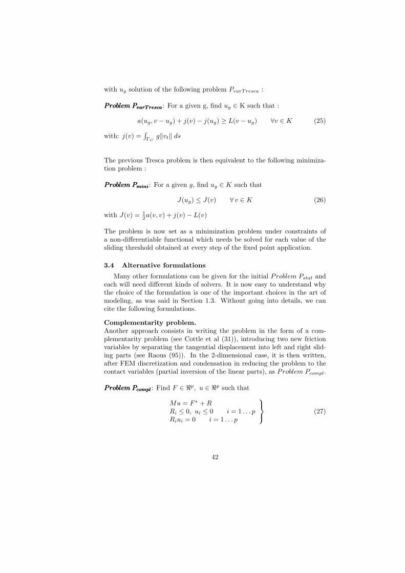
with ug solution of the following problem PvarTresca :

Problem PvarTrescaProblem PvarTrescaProblem PvarTresca: For a given g, find ug ∈ K such that :

a(ug, v − ug) + j(v)− j(ug) ≥ L(v − ug) ∀v ∈ K (25)

with: j(v) =∫ΓC

g‖vt‖ ds

The previous Tresca problem is then equivalent to the following minimiza-tion problem :

Problem PminiProblem PminiProblem Pmini: For a given g, find ug ∈ K such that

J(ug) ≤ J(v) ∀ v ∈ K (26)

with J(v) = 12a(v, v) + j(v)− L(v)

The problem is now set as a minimization problem under constraints ofa non-differentiable functional which needs be solved for each value of thesliding threshold obtained at every step of the fixed point application.

3.4 Alternative formulations

Many other formulations can be given for the initial Problem Pstat andeach will need different kinds of solvers. It is now easy to understand whythe choice of the formulation is one of the important choices in the art ofmodeling, as was said in Section 1.3. Without going into details, we cancite the following formulations.

Complementarity problem.Another approach consists in writing the problem in the form of a com-plementarity problem (see Cottle et al (31)), introducing two new frictionvariables by separating the tangential displacement into left and right slid-ing parts (see Raous (95)). In the 2-dimensional case, it is then written,after FEM discretization and condensation in reducing the problem to thecontact variables (partial inversion of the linear parts), as Problem Pcompl.

Problem PcomplProblem PcomplProblem Pcompl: Find F ∈ ℜp, u ∈ ℜp such that

Mu = F ∗ +RRi ≤ 0, ui ≤ 0 i = 1 . . . pRiui = 0 i = 1 . . . p

(27)

42

where M and F ∗ are respectively a non-symmetric matrix and a loadingvector deduced from the FEM problem by condensation (and taking intoaccount the change of variables associated to the choice of new variables),R and u are the contact forces and the contact displacements, and p isthe number of contact degrees of freedom. This 2D formulation has beenextended to 3D problems using a polygonalization of the Coulomb cone byKlarbring (61).

Penalization formulation for the frictionless contact.The penalization principle consists in adding an extra force Gǫ defined onthe contact boundary to enforce the conditions un ≤ 0; a penalization pa-rameter ǫ is introduced and a nonlinear variational equation is obtained.

Problem PpenalProblem PpenalProblem Ppenal: Find u ∈ U such that ∀ v ∈ U

a(u, v) = L(v) +G(v) (28)

with G(v) =∫ΓC

Gǫ v dsNormal penalization can be considered as a numerical form of the com-

pliance law previously introduced in Section 2.1.

Lagrange multipliers. In that case, the contact force is kept as a variable(Lagrange multiplier). It is a mixed formulation. We get a saddle pointformulation which is a min/max problem.

Augmented Lagrangian. It is a combination of the penalty and the La-grange multiplier formulations.

Details of all these formulations can be found in the books by Laursenand by Wriggers (63) (128) (129).

3.5 Formulations of the quasi-static problem

Coulomb friction law has to be expressed on velocities. It was shownin Cocou-Pratt-Raous (22) (23) (24) (27) and Shillor et al (110) that theproblem is then written as the coupling of two variational inequalities (oneof which is implicit). The problem can be written as follows.

Problem PqsProblem PqsProblem Pqs: For t belonging to [0, T ] and with presribed initial condi-tions, find u(t) ∈ K such that :

a(u(t), v − u(t)) + J1(u(t), v)− J1(u(t), u(t)) ≥ L(v − u(t))+ < Rn(u(t)), vn − un(t)) > ∀v ∈ V

< Rn(u(t)), zn − un(t)) > ≥ 0 ∀z ∈ K

(29)

43

3.6 Formulation of the dynamics problem.

The main contributions to this topic are from Jean-Jacques Moreau (75)(76) for finite dimensional problems (granular medium). In Problem Pstat,the equilibrium equation should be replaced by the equation of motion:

ρ u(x, t) = divxσ(u(x, t)) + φ1(x, t) (30)

As was noted before, in the case of a contact problem, the occurrence ofimpacts and shocks has to be considered and thus the velocities are notcontinuous (and not differentiable). The acceleration cannot be defined inthe usual sense, the notion of differentiable measures has to be used. For thesake of simplicity, we give directly the discrete formulation of the problem.

Problem PdynProblem PdynProblem Pdyn: Find U such that

∀t ∈ [0, T ] U(t) ∈ Vh, U(0) = U0, U(0) = V0 and :

M.dU + K.U + C.U = F + Rdν (31)

and should be satisfied the Signorini and Coulomb conditions for the contactnodes (Section 2.1).dU is a differential mesure representing the discretized acceleration and dνis a nonnegative real mesure relative to which dU happens to possess adensity function. The differential measure is a generalization of the notionof derivative which takes into account the jumps. The derivative u = du/dtis replaced by a differential measure du (Stieltjes measure). In the smoothcase (u is continuous), we have du = udt where dt is the Lebesgue measure,which is in fact the differential measure of the (real) function t. In thegeneral case, for any compact sub-interval [a, b] we have :

∫

]a,b]

dU = U+(b)− U+(a) (32)

with right continuity : U = U+

This formulation in terms of differential measure is the convenient formula-tion to be used for dealing with the jumps and the shocks which may occurin contact dynamics. Convenient numerical methods to solve this problemset under this sophisticated formulation will be given in Section 3.8.

3.7 Mathematical analysis

In this section, we want to stress that some problems could be verystiff, considering the mathematical properties of the operators and of thesolutions.

The art of modeling is then to cope with some choices:

44

• either transforming the initial problem (regularization, etc.) in orderto get a simpler model, easier to solve, but , as was underlined before,the regularized problem is a problem different from the initial one; weshould be aware of that a feature because regularization is currentlyused in most computer codes,

• or addressing the real difficulties of the initial problem, which is noteasy to do, but is the right way to get the correct solutions, even ifthis way is complex.

The mathematical analysis of the non-smooth problems set when modelingcontact phenomena is very important. It is essential for a good understand-ing of the solutions that can be obtained and for overcoming the difficultieswhich arise both in the formulations and in the solvers. As was said inSection 1, a large scientific culture is necessary (either individually or col-lectively as a team). It is impossible to be specialist of everything but itis important to have some knowledge of these various topics, including themathematical topics presented in this section.

Main difficulties and some alternatives.The situation can be summarized as follows.

• The behavior laws are represented by multivalued mapping.Consequence: variational inequalities.Alternative: regularization, but we get a very different problem.

• The Coulomb law is non-associated.Consequence: no minimum principle.Alternative: Tresca problem (as intermediate problem) + fixed pointon the sliding threshold.

• The contact force is a distribution belonging to H−12 (this point will

be addressed below).Consequence: compactness issues arising in the mathematical analy-sis.Alternative: new definition of the contact forces defined by a convolu-tion with a smooth function with compact support (non-local friction).

• For the dynamic problem : impacts result in velocity discontinuities.Consequence: differential measure formulation.Alternative: no alternative in the general case; nevertheless for rigidbody dynamics, restitution coefficients is often used.

Mathematical framework and difficulties.The following scheme (in 3D) gives a synthetic representation of the math-ematical framework for contact problems.This is very helpful to understandthe reasons for the difficulties encountered in the mathematical analysis ofcontact problems.

45

Duality pairings

Contact Uc = H12 (ΓC)

3 (R,w) Φc = H−12 (ΓC)

3

Traceoperator

Displacement U = H1(Ω)3 < Φ, v > ΦF = L2(Ω)3xL2(ΓF )

3

Deformationoperatorǫ = Gradsu

Equilibrium equationsdivσ = −φ1 in Ωσ.n = φ2 on ΓF

Strains E = L2(Ω)9 << σ, ε >> S = L2(Ω)9 Stress

<< σ, ε >>=

∫

Ω

σ(u)ε(v) dx ∀v ∈ U (33)

< Φ, v >=

∫

Ω

φ1v dx+

∫

ΓF

φ2v ds ∀v ∈ U (34)

(R,w) =

∫

ΓC

µ|Rn(u)|‖wt‖ ds ∀w ∈ Uc (35)

This scheme has 3 levels. Levels 2 and 3 (at the bottom) present the classicalscheme for an elasticity problem.

• At level 3, the stress space S and the strain space E are L2(Ω)9; theyare in duality according to the duality product << σ, e >> whichrepresents the work of the stress σ in the strain ǫ,

• At level 2, the displacement space U is H1(Ω)3 and the loading spaceφF should be the dual of H1(Ω)3 for the duality product < φ, v >(which represents the work of the loadings (φ1, φ2) in the displacementu); however, as the loadings are given, we are free to choose them ina more regular space and we choose L2(Ω)3xL2(ΓF )

3 . This is a keypoint for the study of the existence and the uniqueness of the solutionto the mathematical problem set for a small deformation elasticityproblem.

• Level 1 is the level of the contact variables. The situation is similarbut, as the contact forces are unknown, it is not possible to choosea more regular space for them. The contact displacement space U isH

12 (ΓC)

3 (trace of u on the boundary ΓC) and the contact force is in

H−12 (ΓC)

3, which is the dual of U for the duality product (Rc, uc).

H−12 (ΓC)

3 is a distribution space, which will make the mathematicalanalysis more complicated .

46

To complete this schema, we have indicated the mappings acting from onespace to another. Let us note again that each duality product represents awork. This gives a good picture of the mathematical situation.

Introduction of non local friction.In classical elasticity, existence and uniqueness theorems are based on coer-civeness and continuity of the operators, and the proof is based on the Lax-Milgram theorem and Cauchy-Schwarz inequality (equivalence of norms).

In contact mechanics, the first difficulty which arises is that the contactforce is a distribution belonging to H−

12 (ΓC), as explained in the previous

section. This implies some compactness difficulties, and a regularizationRreg using a convolution product is used to overcome this difficulty.

Rreg = R ∗ ψ (36)

where ψ is a very smooth function with compact support (see Duvaut (41)and Cocou (21). Thus, the space for the contact force is much smootherand this will be very helpful for the mathematical analysis:

• R is in H−12 (ΓC), it is a distribution,

• Rreg is in L2(ΓC), it is a function.

However, from a mechanical point of view, it should be noted that thecontact forces are now defined by using a notion of non-local forces.

Overview of the main results about existence and uniqueness ofsolutions.With this overview of the main mathematical results on contact problems,we want to call attention to the consequences of the non-smooth charac-ter of the law. The mathematical difficulties which are pointed out havedirect consequences on the art of modeling, both on the kind of phenom-ena that can be observed and on the computational difficulties that may beencountered.

• Static problem (no mechanical meaning but interesting intermediateproblem). The implicit variational inequality (20) in Problem Pvar

needs to be solved.

– Signorini problem (no friction) (112):existence and uniqueness of the solution - Fichera (44);

– Signorini + Coulomb friction:existence if µ is small and no uniqueness - Necas-Jarusek-Haslinger(79), Jarusek (50), Eck-Jarusek (43);

47

– Signorini + Coulomb (non-local friction):existence and uniqueness if µ is small - Cocou (21), Duvaut (40),Demkowicz-Oden (37);

– Normal compliance + Coulomb friction:existence and uniqueness if µ is small - Klarbring-Mikelic-Shillor(59);

• Quasi-static problem. The two coupled variational inequalities ofProblem Pqs (one of them is implicit) need be solved.

– Signorini + Coulomb:existence if µ is small (both in L∞ and as a multiplier in H−

12 )

and no uniqueness of the solutions - Andersson (5), Cocou-Rocca(26) (105) (106);

– Signorini + Coulomb (non-local friction):existence if µ is small (condition only in L∞) and no uniqueness- Cocou-Pratt-Raous (22) (23);

– Compliance + Coulomb:existence if µ is small and no uniqueness (only a few works) -Andersson (4), Klarbring-Mikelic-Shillor (59);

– Examples of non uniqueness for a discrete problem - Ballard (10).

• Dynamic problem. The Problem Pdyn is formulated in terms of differ-ential measures. There are very few mathematical results in elasticity,more results in viscoelasticity.

– Continuous problem∗ frictionless in elasticity:normal compliance: existence - Martins-Oden (70) (71)Signorini: a few results on specific geometries (axial symme-try) - Munoz-Rivera-Racke (78);

∗ normal and tangential compliance in viscoelasticity:existence and uniqueness - Martins-Oden (70) (71), Kuttler(62);

∗ Signorini problem + non local friction in viscoelasticity:existence - Cocou (28), Cocou-Scarella (29);

∗ Signorini + Tresca friction in viscoelasticity:existence - Jarusek (51);

– Discrete problem∗ existence and uniqueness for analytical loading in 1D

· frictionless - Ballard (11);

· with friction - Ballard-Basseville (12).

48

Concluding remarks on mathematical formulations.Contact and friction relate to non-smooth mechanics: the interface laws aremultivalued mappings, the formulations are written in terms of implicit vari-ational inequalities or differential measures for dynamic problems, in mostcases there is no-uniqueness - and sometimes nonexistence - of solutions,and some problems remain unsolved (no results).

At this point, it is essential to note that the occurrence of multiple so-lutions is not a fantasy of mathematicians: it can really occur. Klarbring(60) and other authors (Janovsky, Alart-Curnier, Mitsopoulos-Doudoumis)constructed very simple examples with a few masses and springs showingthe existence of two solutions, the occurrence of which depends on the val-ues of µ. Unfortunately, the mathematical conditions set on µ depend onmathematical constants such as the coerciveness or the continuity constantsthat cannot be easily evaluated in terms accessible to the designer.

What should be remembered is that multiple solutions may occur andthat the bad conditioning of the problem increases when µ increases. Thisis also observed with the computational resolution. All this is directly con-nected with the mathematical results given above.

From a mechanical point of view, this bad conditioning for large valuesof µ will be observed during the studies on stability. In Section 3.11, thiswill be illustrated with the presentation of a study on the stability analysisof a mechanical system and the search for occurrence of unstable solutionsto modeling squeal phenomena.

In closing this section, we want to underline the strong relationship be-tween mechanics and mathematics, in both directions, that is, from me-chanics to mathematics and vice versa. In mechanics, mathematical toolsare often used while important developments in mathematics have been mo-tivated by the mathematical study of mechanical problems and especiallyof contact mechanics problems; for example, variational inequalities, con-vex analysis, Γ-convergence, etc.. These advances are due to specialistsin theoretical mechanics and mathematicians (mostly by a French-Italianschool and some famous representatives from the USA and Greece). With-out trying to be exhaustive, let us cite Jacques-Louis Lions, Georges Du-vaut, Jean-Jacques Moreau, Panagiotis Panagiotopoulos, Tyrell Rockafellar,Enrico Magenes, Guido Stampacchia, Umberto Mosco, Bernard Nayroles,Pierre Suquet, Marius Cocou, Patrick Ballard, Yves Renard, Patrick Hild,Michelle Schatzman, Laetitia Paoli, etc.). Let us mention the reference bookby R. Dautray and J.L. Lions (33).

Highly theoretical work is still in progress in contact dynamics, alongwith sophisticated mathematical developments.

49

3.8 A short overview of the solvers

The topic is broad and work addressing this topic is still in constantdevelopment. The idea is obviously for this course not to provide an ex-haustive presentation of the solvers used in contact mechanics but to providesome indications and to stress the assumptions that they implicitly make.In fact, we want primarily to draw the attention of the engineer on the carethat must be taken in choosing a solver or in choosing a computer code tosolve a contact problem. It is essential to check what kind of methods areused, what numerical parameters are involved and to make some controltests on the numerical solution.

Details on numerical methods for contact problems can be found for ex-ample in the books byWriggers (128), Laursen (63), Wriggers-Panagiotopou-los (Eds) (127), Wriggers-Laursen (129), Kikuchi-Oden (58). Let us firsthave a look at the methods that are currently used to solve quasi-staticproblems. Some of these methods are commonly used in commercial com-puter codes.

Penalty formulation.As presented in Section 3.4, penalization is a regularization of the strictcontact conditions. An extra force Gǫ, defined on the contact boundary, isadded to enforce the unilateral condition un ≤ 0 and a condition controllingthe friction. Two penalization parameters ǫn and ǫt (shortly noted by ǫ)are introduced. Normal penalization can be considered as a numerical formof the compliance law previously introduced. The functions Gǫ are mostlynonlinear functions with a stiff dependence on the normal penetration intothe obstacle (or sometimes on the vicinity of the obstacle in case of exter-nal penalization) or on the tangential sliding displacement. A nonlinearvariational equation (28) is then obtained. After discretization, a nonlinearproblem needs to be solved and Newton Raphson methods are usually used(see Alart-Curnier (1)).

Au = F +Gǫ(u) (37)

Two remarks have to be made. First, to conveniently ensure the contactconditions the computing parameters ǫn and ǫt have to be chosen in such away that the penalization functions are often stiff and thus the numericalproblem remains hard to solve (bad behaviors of the algorithms). When pe-nalization is soft, computations are easier but contact conditions are thenoften roughly fulfilled. Secondly, as noted in Section 2.1, penalization leadsto an approximation model which is different from the initial model. Thus,two verifications should be done. The first one, relating to the model, is tomake sure that non-smooth solutions are not of interest in the phenomenonstudied (such as oscillations, instabilities, etc.) because they are usually

50

lost when regularization is used. The second one, concerning the numericalsolution, is to check that the values of the penetrations into the obstacleand of the micro sliding amplitudes fit the model objectives and the accu-racy expected for the solution. The regularization drastically disrupts thedetermination of the contact forces.

In commercial computer codes, regularization parameter values are oftenproposed as default values, but specific choices of the function Gǫ(u) (boththe function shape and the parameters ǫc) are generally offered and it isrecommended to use them. It will be observed that the choices of thepenalization parameters improving the quality of the solutions often lead tolarge computational times. In any cases great care is recommended whenregularization is used.

Lagrange multiplier formulation.In that case, the contact force is kept as a variable (Lagrange multiplier).It is a mixed formulation. This method permits an accurate determinationof the contact forces. We get a saddle point formulation which is solvedby using the Uzawa algorithm (min/max optimization). It should be notedthat additional variables (the contact forces) have to be introduced in thatcase (larger number of DOF).

Augmented Lagrangian formulation (widely used).(see Simo-Laursen (114))It is a combination of the penalty and the Lagrange multiplier formulations.An iterative process is used to reach the correct value for the multiplier(number of augmentations). The augmentation consists in adding a pe-nalization term. The case with only one augmentation corresponds to theusual penalization. We get a variational equation coupled with the condi-tions of contact and friction (Kuhn Tucker conditions). A Newton Raphsonmethod, which depends on the number of augmentations, is combined witha radial return process for the contact. For friction, stick prediction is doneand correction is conducted for sliding when it is needed.

This method is very powerful and very often used in the computer codesdeveloped in academic research laboratories.

We present now numerical methods solving the strict conditions for uni-lateral contact and friction. Details can be found in Raous (95), Raous etal (92), Chabrand et al (16), Lebon-Raous (64), Klarbring-Bjorkman (61).

Lemke method (complementarity problem).The complementarity formulation of the contact problem complying withthe strict contact conditions was given in section 3.4 (see Klarbring-Bjork-

51

man (61), Raous (95) (90), Cottle et al. (31)).

Methods derived from mathematical optimization, such as the Lemkemethod or the interior point method (see (20) (61)) can be used. TheLemke algorithm is a mathematical programming method. It is a directmethod based on pivoting techniques, similar to the Simplex method.

In elasticity or for linearized behaviors, a condensation of the problemcan be conducted in order to write the problem only on the contact vari-ables. This is done by a partial inversion of the total system that can beperformed not by inverting the global matrix but by solving (only once atthe beginning) a set of linear problems. Details are given in Raous (95), anextension to treat dynamic problems is given in Vola et al (122). Then theLemke method is applied on the reduced system whose rank depends onlyon the number of contact nodes. It is however a full sized matrix whichis non-symmetric (because of the friction). Using a direct method is verycomfortable; the number of pivotings is less than the rank of the matrix(and in practice much more less). However, because of the full sized matrix,this process cannot be used for huge numbers of DOFs. In that case, whensubdomain or multigrid methods are used, the Lemke method turns out tobe still very efficient for coarse grids (see Lebon et al. (65)).

Fixed point on the sliding limit and minimization problem.It has been shown that the variational inequality problem (strict contactconditions) can be set as a sequence of minimization problems combinedwith a fixed point method on the sliding limit. At each step, we solve aTresca problem, i.e., a frictional problem where the sliding limit is given.The Trescas law being an associated law, a minimum principle can be asso-ciated. The iteration on the sliding limit converges quite fast (less than 10iterates and often less than 5) depending on the size of the system and onthe prescribed accuracy. Details can be found in Raous (95).

We have to solve Problem Pmini which is a minimization problem underconstraints (u belongs to the convex K) of a non-differentiable functional.Various minimization methods with projection can be used.

• Successive Over Relaxation and Projection (SORP). An optimal pa-rameter of relaxation has to be determined using a trial procedure.The method is very robust but can be costly when extension to non-linear problems is considered.

• Gauss-Seidel with Aitken acceleration. No numerical parameter isneeded.

• Pre-conditioned conjugate gradient with projection (see Raous-Barba-rin (93)). This is a very powerful method but a regularization of thefriction term has to be done in order to evaluate the gradient of thefunctional to determine the descent directions.

52

Multigrid methods. see Lebon-Raous-Rosu (65).As noted before, we have developed multigrid methods for solving contactproblems without regularization of the contact, i.e., using the strict Signoriniconditions and the strict Coulomb law.

Multigrid methods operate at several levels of meshes (usually 2 to 5levels) which are coarser than the initial mesh where the solution will becalculated. This is an iterative process using complete resolutions on thecoarsest grid and a few smoothings conducted on the default of equilibriumon the intermediate grids. At each iteration, the Lemke method can be usedon the coarsest grid to solve the small sized problem, and the projectedGauss Seidel method will be a very efficient smoother on the other finergrids.

In all the examples presented in this course, for both quasi-static anddynamic problems, no regularization of the contact conditions was usedand the algorithms fitted the non-smooth character of the laws. This isfundamental for modeling specific phenomena such as squeal, which is dueto the occurrence of unstable solutions for the theoretical problem.

Dynamics problem.As presented before, because of the non-derivability of the solutions (shocks),the problem has to be formulated in terms of differentiable measures: equa-tion (31).

A classical Newmark method which is based on a limited development ofthe solution needs their derivability and cannot be used. However, some im-provements have sometimes been developed to adapt the Newmark methodto the problem (usually some numerical damping). But, we should be awarethat the use of numerical damping will kill not only numerical oscillates butalso some real solution oscillates (flutter for example).

A specific method called the Non-Smooth Contact Dynamics (NSCD)method was developed in Montpellier by Moreau-Jean-Dubois (52) (53) fordiscrete problems (granular materials). A version adapted to continuousformulations and FEM was conducted at the LMA in Marseille - Jean et al(54). The system on differential measure (31) can be written in the followingequivalent form: ∀t ∈ [0, T ]

M(U(t)− U(0)) =

∫ t

0

(F −K.U − C.U)ds +

∫

[0,t]

Rdν (38)

U(t) = U(0) +

∫ t

0

Uds (39)

53

where ds represents the Lebesgue measure. Be given the time discretization:i = 0...N, ti = i.h (h is the time step), (38) is written:

M(U(ti+1)− U(ti)) =

∫ ti+1

ti

(F −K.U − C.U)ds +

∫

[ti,ti+1]

Rdν

and

Ri+1 =1

h

∫

[ti,ti+1]

Rdν.

To complete the time discretization the two following Lebesgue integralsmust be approximated :

∫ ti+1

ti

(F −K.U − C.U)ds and

∫ ti+1

ti

Uds.

The choice of the integration methods must be influenced by the fact thatthe velocity is discontinuous. We have used the following three methods:

• θ-Method : both integrals are approximated by the classical θ-methodi.e. where:∫ ti+1

ti

fds ≈ h(θf(ti+1) + (1− θ)f(ti)) ,

• θ-Euler-Method: the first integral is approximated by the θ-methodand the second one by the Euler implicit method,

• modified θ-Method: both integrals are approximated by the θ-methodbut in the contact relations the displacement u(ti+1) is replaced byu(ti+1) = u(ti+1) + h(1− θ)u(ti+1).

In contact and multibody dynamics, we have to mention the referencebooks by Pfeiffer-Schindler (88), Pfeiffer (87) and Pfeiffer-Glocker (86).

3.9 Numerical analysis

In the art of modeling, it is important to keep in mind the three stepsbetween the initial mathematical problem and the final solution given bythe computer code, and consequently the three levels of the analysis.

• The initial continuous problem is set in functional spaces (Hilbertspaces in our case; see Section 3.1).

• This problem is approximated by an approached problem set in fi-nite dimensional spaces; when FEMs are used these finite dimensionalspaces are generated by a basis of functions constructed on the finiteelement mesh; this problem is still written in functional spaces (L2).

• The discrete problem is deduced from the previous one, which is writ-ten in ℜN .

54

Numerical analysis is applied to the study of the properties of the solu-tions to these various problems and the relationship between these solutions.It is a mathematical task. An important feature is the convergence (andthe order of convergence) of the approximated problem towards the initialcontinuous problem when the size of the refinement (element size) goes tozero. Numerical analysis is also applied to the study of the convergence ofthe algorithms and the evaluation of the computational errors.

Numerical analysis is of great importance in the art of modeling andconstitutes a huge part of applied mathematics. It will help the engineer tochoose and control the numerical methods, the algorithms and the numericalparameters.

Once again, it is not possible to be a specialist in all these topics butbearing the main numerical analysis results in mind will be very helpful toconduct a coherent modeling process.

In contact mechanics, among a number of studies, we can cite those byGlowinski- Lions-Tremolires (46) and Barbara Wohlmut (125).

3.10 Conclusions

The interaction between mechanics and mathematics is of great impor-tance in the art of modeling mechanical systems. It concerns not only theway to set and to write the problems (choice of the formulation) but also theway to solve it. Mathematical results which could sometimes be very toughto analyze are in fact of great interest for understanding some subtlenessof the models and of the solutions, and also very helpful for choosing andcontrolling the numerical methods.

In the light of the mathematical analysis briefly presented in this section,we can stress a few points in contact mechanics modeling:

• Contact problems are relevant to non-smooth mechanics. The non-smooth character of the basic laws (Signorini, Coulomb), beyond thesimplicity of these laws, contains the ingredients for modeling manymechanical phenomena observed with frictional contact. This non-smooth character should be preserved and studied properly; regular-ization should be avoided as much as possible because using regular-ization may result in some fundamental mechanical properties beinglost.

• When the friction coefficient µ is large, the problem becomes ill-posedand things take a bad turn, both for theory and for computations.Multiple solutions may occur and it is even possible to construct ex-amples with a few degrees of freedom showing the existence of several

55

solutions when µ is large. The convergence of some of the algorithmsis distorted when µ is large.

• Therefore, when it comes to friction modeling it is very important tokeep in mind that: - when the friction coefficient µ tends to zero, theproblem will tend towards a tangential free boundary condition, asintuition suggests, - but when friction µ tends to infinity, the problemdoes not tend towards a tangential clamped boundary condition (asintuition could suggest) but towards a very bad conditioned problemwhere strange phenomena may occur (multiplicity of solutions, flutter,divergence, etc.). For example, we will show in the next section thata ”large µ” makes easier the occurrence of instabilities

3.11 Friction instabilities: a model to reduce squeal of a rubber-like waist seal sliding on a car window

With this example we would like to emphasize various points earlieraddressed about the art of modeling:

• how much theoretical and mathematical analysis is helpful to solveindustrial problems,

• making it as simple as possible when choosing the model (a constantfriction coefficient is used),

• avoiding regularization in order to preserve the non-smooth characterof the laws which is fundamental here (strict contact conditions areprescribed),

• using convenient tools for solving the Non-Smooth Contact Dynamicproblem (the NSCD method).

The industrial problem.The problem is to optimize the design of a waist seal in order to reduce orto avoid the squeal phenomena observed during the sliding of this waist sealon a lateral car window. Mainly, we have three constitutive characteristicsto optimize: shape of the waist seal, rubber, varnish (that is, the frictioncoefficient). Because of the strong nonlinearities of the problem, optimiza-tion through an experimental trial/error process like the one mentioned inSection 1.1 cannot be used (too many experiments to perform).

Modeling has two goals: understanding the reasons for the occurrenceof the nuisance and constructing a simulation tool to help the engineer inthe design of a new seal.

Model and assumption.Details on this study conducted within a collaboration with J.A.C. Martinsat the IST of Lisbon can be found in Raous et al (98), Martins et al (72),Vola et al (123). See also the work conducted by N Guyen Quoc Son (80)

56

and Franck Moirot and Xavier Lorang on stability analysis with applicationto brake squeal.The work was done in several stages.

• First a mathematical analysis of friction stability was conducted in(72). Theorems giving the sufficient or necessary conditions for insta-bility to occur (under a set of assumptions) in linear elasticity wereestablished.

• Secondly, an extension of the analysis of the stability in finite deforma-tion and nonlinear elasticity (Mooney-Rivlin) was established in (123).This was again a theoretical work. Computational tools for solvingthis nonlinear and non-smooth problem were developed on the basisof the NSCD method (see Section 3.8).

• The theoretical conditions for the instability to occur was interpretedon the discrete problem as generalized eigenvalue analysis on certainmatrices which depend on the contact condition and have to be up-dated all along the solution evolution.

• Finally, the model was applied to the industrial problem.

Mathematical analysis of instability for frictional contact.The analysis of instability for frictional problems is a difficult and still veryopen problem. In the present contribution, we set a basic assumption whichis that there is no change in the sliding condition when instability occurs.This means that a point sliding in one direction can oscillate but withoutreverse sliding, only with changes in the velocity amplitude. This assump-tion permits a local linearization for conducting the stability analysis. Thisassumption seems to be very restrictive but it will be observed finally thatwhen the dynamic solution is computed, instability occurrence satisfies thecondition given by the following theorems. This suggests that these condi-tions could be considered quite optimal despite this initial very restrictiveassumption.

The regular solutions are computed. In (72), we are interested in the ini-tial condition problem, i.e., a Cauchy problem. In (123), we are interestedin the steady sliding solution for modeling the sliding of a waist seal on awindow glass. In order to study the stability of these solutions we introducea perturbation and we evaluate the perturbed solution. The stability anal-ysis depends on the contact status (no-contact nodes, sliding nodes, stucknodes) either of the steady sliding solution or at every time steps of theregular solution. In every case, the possible growth of the perturbed solu-tion is computed by considering the admissible directions depending on thecontact conditions. Generalized eigenvalue problems are obtained. Detailsof the stability analysis can be found is the papers previously referenced. Aseries of theorems giving either necessary or sufficient conditions for flutteror divergence instability are then established.

57

Numerical analysis of the stability.These theorems are interpreted on the discrete problem (FEM) as the anal-ysis of generalized eigenvalue problems set on matrices which depend on thecontact status of the solution (non-contact nodes, sliding nodes and stucknodes).

The discussion is conducted both on the rate growth of the perturbedsolution (real positive part of the complex eigenvalues) and on the frequencyof the flutter (imaginary part of the eigenvalues).

Let us summarize the modeling process:

• let us first emphasize that we use contact and friction models withoutregularization and with a constant friction coefficient

• we compute the regular solutions, either Cauchy solution or steadysliding solution (small or finite deformations, linear or nonlinear elas-ticity, etc.)

• stability analysis is conducted on the generalized eigenvalue problemsset on matrices depending on the contact condition.

• in order to evaluate the optimality of the conditions, computationof the dynamic solution using the Non Smooth Contact Dynamicsmethod is conducted in the situation where instability is predicted tooccur by the theory.

Application to the waist seal.Two specimens of waist seals are considered (see Fig. 37). For each, thepossible occurrence of squeal is studied relative to the variation of the mainconstitutive parameters (especially the friction coefficient). This consistsin analyzing the generalized eigenvalue spectra. Validation of the model isconducted by comparing the model results and the results of experimentsconducted by Renault. We will compare the two specimens presented inFig. 37 and evaluate for each of them the possibility of squeal to occur byanalyzing the eigenvalue spectrum.

First the steady sliding solution is computed for a glass window mov-ing up and moving down for various values of the friction coefficient (finitedeformations, rubber nonlinear elasticity, unilateral contact and friction)given in Fig.37. For each we need to build some matrices depending onthe contact condition (see (96), (72), (123) for details). Generalized eigen-value problems are solved. To analyze the flutter instability occurrence, theimaginary part is interpreted in terms of frequencies (see Fig. 38 and 39),the real part in terms of growth rates. The eigenmodes are also computed.A large number of results are given in (123). We only present on Fig. 38and 39 the spectra of the flutter instability which may occur for each of thetwo geometries in function of the values of the friction coefficient. It can be

58

noted that in the acoustic range (100Hz 14 000Hz), geometry 1 generates aflutter vibration (2000Hz and 14 000 Hz) for µ > 0.3, although in the samerange 0.3 < µ < 0.45 geometry 2 is stable, flutter does not occur.

Then, when the dynamics evolution of the perturbed solution is com-puted using the NSCD method for µ = 0.4 for the two geometries, a growingoscillating solution (flutter) for geometry 1 and a stable solution for geome-try 2 can be observed (see Fig. 40 and Fig. 41). This confirms that despitethe very strong assumption made at the beginning of the stability analysis,the stability conditions seem to be quasi optimal.

This is validated by the experiments which show that geometry 2 is morestable (no squeal) than geometry 1 and when flutter occurs with geometry1, the frequency of the squeal noise is about 2000Hz.

Figure 37. The two specimens: steady sliding solutions (deformation and forces)for a glass window moving up and moving down

0.0 0.05 0.1 0.15 0.2 0.25 0.3 0.35 0.4 0.45

Friction coefficient0

2000

4000

6000

8000

10000

12000

14000

16000

18000

20000

Flut

ter

freq

uenc

y(H

z)

Figure 38. Flutter frequencies (geometry 1, glass moving up, µ = [0, 0.45]).

0.0 0.05 0.1 0.15 0.2 0.25 0.3 0.35 0.4 0.45

Friction coefficient0

2000

4000

6000

8000

10000

12000

14000

16000

18000

20000

Flut

ter

freq

uenc

y(H

z)

Figure 39. Flutter frequencies (geometry 2, glass moving up, µ = [0, 0.45]).

59

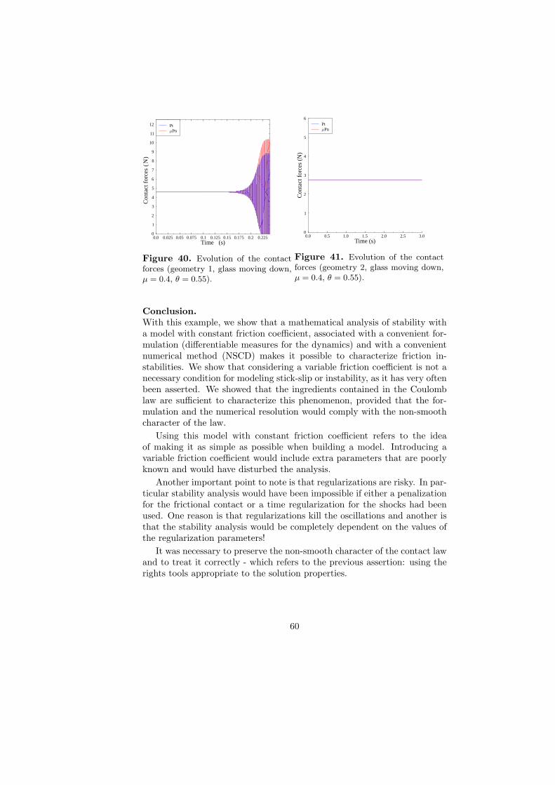
0.0 0.025 0.05 0.075 0.1 0.125 0.15 0.175 0.2 0.225Time (s)

0

1

2

3

4

5

6

7

8

9

10

11

12

Con

tact

for

ces

(N

)

PnPt

Figure 40. Evolution of the contactforces (geometry 1, glass moving down,µ = 0.4, θ = 0.55).

0.0 0.5 1.0 1.5 2.0 2.5 3.0Time (s)

0

1

2

3

4

5

6

Con

tact

forc

es(N

)

PnPt

Figure 41. Evolution of the contactforces (geometry 2, glass moving down,µ = 0.4, θ = 0.55).

Conclusion.With this example, we show that a mathematical analysis of stability witha model with constant friction coefficient, associated with a convenient for-mulation (differentiable measures for the dynamics) and with a convenientnumerical method (NSCD) makes it possible to characterize friction in-stabilities. We show that considering a variable friction coefficient is not anecessary condition for modeling stick-slip or instability, as it has very oftenbeen asserted. We showed that the ingredients contained in the Coulomblaw are sufficient to characterize this phenomenon, provided that the for-mulation and the numerical resolution would comply with the non-smoothcharacter of the law.

Using this model with constant friction coefficient refers to the ideaof making it as simple as possible when building a model. Introducing avariable friction coefficient would include extra parameters that are poorlyknown and would have disturbed the analysis.

Another important point to note is that regularizations are risky. In par-ticular stability analysis would have been impossible if either a penalizationfor the frictional contact or a time regularization for the shocks had beenused. One reason is that regularizations kill the oscillations and another isthat the stability analysis would be completely dependent on the values ofthe regularization parameters!

It was necessary to preserve the non-smooth character of the contact lawand to treat it correctly - which refers to the previous assertion: using therights tools appropriate to the solution properties.

60

4 Identification, validation and validity domain -

examples

Model validation constitutes a fundamental step in the model-building pro-cess before using the model for predicting new behaviors. Parameter iden-tification is an intermediate step which only shows that there exists at leastone set of parameters that provides a good description of a reference ex-periment, no more. The validation must show that the model using thepreviously determined constitutive parameters can give a good simulationof other experiments than the one used for the identification. Then, pre-diction consists in using the model in situations where no experiments havebeen carried out. The examples considered (geometries, load amplitude,load velocities, etc.) have to be compatible with the founding model as-sumptions (validity domain). As presented below, contact mechanics oftenrequires specific procedures. This will be illustrated by several examples.

4.1 Validation of the numerical methods

The first issue is the validation of the numerical method used to solve theproblem. It consists in verifying that the numerical tools have been correctlychosen and implemented, and evaluating the errors they introduce.

In contact mechanics, we need to check first if the solution fulfills thecontact conditions: no penetration (or small penetration if penalization isused), only traction on the contact boundary, condition ‖Rt‖/|Rn| = µwhen sliding occurs, etc. Besides that, as usual, a more complete analysishas to be conducted to check the ability of the numerical method to correctlysolve the problem.

The validation of a numerical method could be conducted using:

• an analytical solution when it is possible (it is the best way but is notalways possible with a complex model),

• a Benchmark which is a reference example chosen by a user commu-nity which permits comparisons of the results obtained using variouscomputational codes as well as discussions between developers. Thismeans that a consensus has emerged within the scientific communityto consider a solution as a reference solution. The characteristics of aBenchmark should be the same as those of the problem under consid-eration: kinematics, material behavior, load type, etc.

Analytical solutions for contact problems are rare and limited to ba-sic cases: small deformations, elastic behaviors, simple geometries (sphere,cylinder, contact with a half-plane), simple loadings (static contact, inden-

61

tation, etc.) and often frictionless contact. In contact mechanics, very oftenwe will have to use benchmarks.

This validation of the numerical method is essential. It is absolutely re-quired when developing a new method, and it is also recommended and veryuseful when using an existing method (in a commercial code for example).Furthermore it also constitutes a way to evaluate the performances of thealgorithms:

• to test the convergence,

• to evaluate the errors (and to compare them with the theoretical es-timates),

• to adjust the computational parameters and test the sensitivity of thesolutions to their variation,

• to compare the efficiency of various methods.

Example: validation of the computational methods for solving thecontact problem of a rubberlike structure with unilateral contactand friction.An extension of the NSCD method presented in Section 3.8 was developed tocompute the dynamic solution of the problem presented in Section 3.6. Thisnew method was built to solve problems of unilateral contact with Coulombfriction (without regularization) for a rubberlike material with large defor-mations and non-linear elasticity (with incompressibility condition). Theproblem is too complex to provide a reference analytical solution which canbe used to validate the method. Two Benchmarks were considered, one forquasi-static loading and one for dynamic loading.

Computation of the quasi-static compression of a cylinder.This Benchmark was proposed and used by Simo-Taylor (113), Sussman-Bathe (117) and Liu-Hofsetter-Mang (68). Cases without friction and withfriction (µ = 0.2) were considered (see Fig. 42, 43 and 44)

There was very good agreement between our results and those obtainedby Sussman-Bathe (117) (displacement/hydrostatic pressure formulation)and Simo-Taylor (113).

Dynamic impact of a cylinder inside a cone.This Benchmark was proposed by Wriggers et al (126). It is the impact of arubberlike cylinder inside a rigid cone. A good agreement was also obtained(Vola et al (123)).

With these examples, we stressed the importance of validating the nu-merical methods associated with a model and the difficulties finding a ref-erence test in the case of complex problems.

62

U=0.32m

U=0.25m

U=0.2m

Figure 42. Deformations forthe frictionless case

0.0 7.5 15.0 22.5 30.0Displacement (mm)

0

400

800

1200

1600

2000

2400

Nor

mal

cont

actf

orce

(N)

Rn frictionless case

Figure 43. Resultantcontact forces for µ=0

0.0 7.5 15.0 22.5 30.0Displacement (mm)

0500

1000150020002500300035004000450050005500600065007000750080008500

Nor

mal

cont

actf

orce

(N)

Rt frictional caseRn frictional case

Figure 44. Resultantcontact forces for µ=2

initial velocity1.5m/ s

40 deg

r=9mmR=10mm

node 1

Figure 45. impact of a cylinder intoan angle

=0.3 =0.5

Frictionless case =0.1

Figure 46. Deformation of the cylin-der and contact forces for various fric-tion coefficients.

4.2 Identification of the constitutive parameters.

As earlier noted, mechanics of materials and structures, it is usually pos-sible to determine the constitutive parameters with preliminary and stan-dard experiments conducted on specimens. However, for contact problems,the identification of the constitutive parameters (and especially the frictioncoefficients) is very difficult because of the strong dependence on the en-vironmental conditions (temperature, surface condition, residual lubricant,etc.). Special methodologies are needed; for example conducting the identi-fication on the mechanical problem itself (the complete structure) taking agiven loading situation as reference. Once this is done, the validation of themodel will be conducted on other cases of loadings by using the parametersdetermined during the identification.

63

It should be kept in mind that identification of the constitutive param-eters is an important and difficult task. It is a key point in the art ofmodeling. It is a problem of minimization of the error between the exper-iment and model results. As said earlier, the choice of error norm is veryimportant (L2 or L∞ for example). This minimization problem does nothave a unique solution (a priori no convexity property of the functional tominimize). We have to deal with local minima and so the search for the cor-rect parameters has to be enriched by estimations of ranges of values basedon mechanical considerations. We will illustrate this with a few examplesin Sections 4.4, 4.5 and 4.6.

4.3 Validation of the model.

Now that the numerical methods are validated and the constitutive pa-rameters evaluated, model validation will consist in verifying whether themodel using the previously determined parameters is able to describe otherexperiments. The experimental conditions have to satisfy the constraintscreated by the validity domain conditions of the model. The norm used toevaluate the error between simulation and experimental results should bethe same as the one used for the identification. This will be commented andillustrated with the following examples.

4.4 Example in Mechanics of Materials: cyclic behavior of poly-meric foam.

The construction of a model for the cyclic behavior of polymeric foamwas presented in Section 1.9. Here, we give details about the identifica-tion step and highlight some specific ways to proceed (see Pampolini-Raous(82)). The model uses a number of parameters (to characterize viscosity,nonlinear elasticity and damage) and we will stress two points:

• the number of parameters should be minimized (as few as possible andas many as necessary): to characterize the viscosity, we will minimizethe number of relaxation times to be taken into account,

• mechanical considerations should be included in selecting the param-eters of the nonlinear elastic model, instead of conducting a blindedminimization process.

Identification of the viscosity parameters.The relaxation times characterizing the viscosity were identified using ex-tra relaxation experiments conducted on foam specimens. The relaxationcurves give the evolution of the stress when an initial deformation is pre-scribed and kept constant. The problem is to determine the number of

64

420 10000 10000004

5

6

7

8

Time (s)

Str

ess

(kP

a)

Figure 47. Relaxation experiment lasting 10 days: comparison of a model with4 exponentials (dotted line) and 5 exponentials (full line) with the experimentalcurve which is indistinguishable from the full line one.

Zener/Maxwell moduli and the values of the associated constitutive param-eters, which will make it possible to simulate these relaxation experimentsproperly. It can be shown that the problem reduces to approximate theexperimental curves by a series of exponentials. The corresponding mini-mization problem is solved by combining an interpolation method (Pronymethod) and a minimization method (Hooke and Jeeves). For a model tobe as simple as possible, we start with one modulus and make the identifi-cation, i.e., we determine the best values of the parameters to minimize thegap between theory and experiment. This gap remains large when only onemodulus is used and so we progressively increase the number of moduli inorder to take the smallest number of moduli needed to get a good approx-imation of the relaxation curve. This is presented in Fig. 47. Long periodeffects (recovery effect after a resting period) and short ones (during a cycle)coexist. Thus, very different relaxation times were identified. It turned outthat five Zener/Maxwell moduli (i.e. ten parameters) were sufficient (andnecessary!) to get a good description of the viscoelastic effect.

Identification of the parameters of the nonlinear elasticity.Once the viscosity parameters were identified using the relaxation exper-iments, those of the nonlinear elastic springs were identified for the firstloading cycle. Six parameters characterize the shape of the strain energygiven in Fig. 6 : c, µ,m, β, k, a. Instead of conducting a blind optimization,we analyzed first the role of each constant in the response curve (σe, ǫ) ofthe nonlinear spring (Fig. 6 in Section 1.9). It can be seen from Fig. 48that:

• c determines the initial slope and the value of the local maximum -Fig. 48(a);

• µ determines the second ascending branch - Fig. 48 (b);

• m determines the descending branch, the position and the value ofthe local maximum - Fig. 48 (c);

65

• when β increases, σe decreases when ǫ ≃ a - Fig. 48 (d);• k determines the slope of the curve when ǫ ≃ a - Fig. 48 (e);• a determines the position of the local minimum - Fig. 48 (f).

0 0.2 0.4 0.60

2

4

(a)

ε

σe[kPa]

c=76

c=85

c=94

0 0.2 0.4 0.60

2

4

(b)

ε

σe[kPa]

µ=2.3

µ=2.5

µ=2.7

0 0.2 0.4 0.60

2

4

(c)

ε

σe[kPa]

m=13.5

m=15

m=16.5

0 0.2 0.4 0.60

2

4

(d)

εσe[kPa]

β=3

β=3.3

β=3.6

0 0.2 0.4 0.60

2

4

(e)

ε

σe[kPa]

k=16

k=18

k=20

0 0.2 0.4 0.60

2

4

(f)

ε

σe[kPa]

a=0.36

a=0.4

a=0.44

Figure 48. Nonlinear elasticity model: influence of the constitutive parametervariation on the stress/strain curve.

After this preliminary analysis, the identification procedure was performedon numerical simulations of a complete loading/unloading cycle (Fig. 49).The following procedure was used for this purpose:

1. select c to obtain the initial slope of the experimental curve;2. select m (with c being fixed) to obtain the appropriate value of the

force at the beginning of the plateau regime;3. select µ (with c and m being fixed) to obtain the appropriate value of

the force at the end of the loading process (ǫ = 0.7);4. perform an optimization routine with the Hooke and Jeeves method

to determine the values of a, β and k.

The parameter characterizing the damage evolution is then identified frommulti-cycle experiments. The final results are given in Fig. 49 and Fig. 50(model results in full line; experimental ones in dotted line).

66

0 0.1 0.2 0.3 0.4 0.5 0.6 0.70

2

4

6

8

10

Deformation

Str

ess

(kP

a)

Figure 49. Theory/experiment com-parison when using the nonlinear elas-ticity model with viscosity

0 0.1 0.2 0.3 0.4 0.5 0.6 0.70

2

4

6

8

10(b)

Deformation

Str

ess (

kP

a)

Figure 50. Theory/experiment com-parison when using the model with non-linear elasticity, viscosity and damage.

Validation of the modelIn this example, model validation was achieved through simulation of com-plex loadings using the same values of the constitutive parameters (thoseresulting from the identification): cycles with various amplitudes, cycleswith intermediate unloadings, etc. Results can be found in Pampolini et al(82).

4.5 Example in Mechanics of Materials : fiber/matrix interfacein a composite material

With this example of micro-indentation of a single fiber in a SiC/SiCcomposite, which was presented in Section 2.4, we stress the importance ofthe mechanical analysis during the identification process.

This experiment was conducted in order to identify the constitutive pa-rameters of the RCCM model which was developed to describe the behaviorof a fiber/matrix interface. As presented in Section 2.4, the RCCM modelhas four parameters: the friction coefficient µ, the initial stiffness of theinterface C (Cn = Ct), the adhesion energy ω (the Dupre energy) and theinterface viscosity b.

Again, the identification procedure was not performed as a blind opti-mization. Preliminary studies were conducted to get a range of admissiblevalues for each parameter. Extra experiments and energetic analysis wereconducted: creep analysis (when the prescribed displacement keeps a con-stant value at the end of the indentation) and cyclic loading/unloadingdisplacement of the indenter.

These preliminary studies based on mechanical considerations and some

67

elementary computations provide:

• an estimate of the initial stiffness of the interface based on the thick-ness and the properties of the third body present in the interface (thefiber envelop which is a pyrolytic carbon);

• an estimate of the friction coefficient based on the analysis of dissipa-tion during a cycle;

• a range of possible values for the adhesion energy ω based on thevalues of Dupre energy for these materials and energetic analysis;

• an estimate of the order of magnitude of b through experiments withdifferent values of the indentation velocity coupled with the creepanalysis.

On the basis of these preliminary estimates, the precise values of the param-eters were identified using the experimental curve given in Fig. 51. Detailscan be found Raous-Cangemi-Cocou (95) (96).

. .. ........

............

. ..

..

..

.

0.0 0.5 1.0 1.5 2.0 2.5 3.0Displacement of the indentor ( m)

0.0

0.1

0.2

0.3

0.4

0.5

0.6

0.7

Forc

eon

the

inde

ntor

:F(N

ewto

n) . experimentnumerical : adhesion alonenumerical : friction alonenumerical : adhesion and friction

Figure 51. Identification of the constitutive parameters on an indentation ex-periment - Experiment (full line) - RCCM model (star line)

Validation.Validation of the model was conducted through experiments with fibers ofvarious diameters and different loadings.

68

4.6 Example in Civil Engineering: steel/concrete interface inreinforced concrete

With this example, we illustrate the ultimate step of the construction of amodel (see Section 1.7): when the best simulation that can be obtained afteridentification of the parameters is not satisfactory, the model needs to beimproved, i.e., new ingredients have to be introduced, and extra phenomenataken into account.

This is a civil engineering problem: modeling the behavior of the steel-concrete interface in reinforced concrete. The RCCM model was used tosimulate the interface and an experiment consisting in pulling out a steelbar embedded in a concrete specimen was conducted (see Raous-Karray(101) (57)). The mesh is presented in Fig. 52.

Adh

esio

n zo

ne

pull

Figure 52. Pull-out of a steel bar from a concrete specimen experiment: themesh

Identification.During the identification process, using the standard RCCM model it wasimpossible to determine the values of the four parameters (µ,C, ω, b) whichcould give a correct simulation of the experiment: we got either a gooddescription of the peak or a good description of the asymptote (see Fig.54).The friction coefficient µ was the key parameter. Therefore, we introduceda friction coefficient depending on the sliding displacement (see Fig. 53).From a mechanical point of view, this corresponds to taking into accounta wear phenomenon corresponding to the grinding of the interface whensliding occurs, due to the powdery nature of concrete. The debris generatedat the interface act as lubricant and the friction coefficient decreases whensliding occurs.

Then, it was possible to find values of the constitutive parameters C, ω,b and those defining the variation of µ given in Fig. 53 to obtain a verygood approximation of the experimental result (see Fig. 55).

69

0.0 0.5 1.0 1.5 2.0 2.5 3.0 3.5 4.0 4.5 5.0 5.5 6.0Deplacement (mm)

0.0

0.05

0.1

0.15

0.2

0.25

0.3

0.35

0.4

0.45

0.50.0 0.5 1.0 1.5 2.0 2.5 3.0 3.5 4.0 4.5 5.0 5.5 6.0

Loi utilisee pour mu variable

0.0

0.05

0.1

0.15

0.2

0.25

0.3

0.35

0.4

0.45

0.5

Figure 53. Variation of the friction coefficient related to the sliding displacement

Figure 54. Approximation of the ex-perimental curve (diamond line) by theregular RCCM model with µ = 0.28 andµ = 0.46.

Figure 55. Approximation of the ex-perimental curve (square line) by themodel with variable friction coefficient

Figure 56. Simulations (full line) andexperimental results for 3 rods of diam-eter 14mm (squares), 12mm (triangles)and 10mm (circles).

Figure 57. Simulations (full line) andexperimental results for 3 lengths of theadhesive zone: 15cm (diamonds), 10cm(squares) and 5cm (circles).

70

Validation.Validation of the model was performed by conducting experiments on rodsof different diameters and on specimens with contact interfaces of differentlengths . The results presented in Fig. 56 and 57 show the good agreementbetween the model simulation and the experimental results. This validatesthe model and in particular the choice of the function µ(ut) given in Fig.53.

4.7 Conclusion

Using these examples, we stressed that identification of the constitutiveparameters of a model could be a difficult task (especially in contact me-chanics). It is not a simple optimization problem. It is very importantto take into account the mechanical meaning of the parameters as well asthe range of their possible values. Complementary experiments and spe-cific protocols may be needed (in Section 4.4, both relaxation and cyclicloadings were used and an ordered sequence was defined for the parameterdetermination).

In contact mechanics, identification and validation are often conductedwith the same kind of experiments and special care should be brought tothe processes which are conducted and to the experiments which are chosenin the two cases.

As said at the very beginning, identification of the constitutive parame-ters and validation of the model are two key steps to get an efficient modelfor simulating and predicting the behavior of a mechanical system while itis sometimes considered that the only noble part in the art and craft ofmodeling is the construction of the model.

What we have tried to show in this last chapter is that not only areconstitutive parameter identification and model validation two key pointsin the art of modeling, they also are real scientific approaches.

Bibliography

[1] P. Alart, A. Curnier, A mixed formulation for frictional contact problems proneto Newton like solution methods, CMAME, 92(3),353-375, 1991.

[2] G. Anciaux, J.-F. Molinari, Contact mechanics at the nanoscale, a 3D multi-scale approach, IJNME, 79(9), 1041-1067, 2009.

[3] G. Anciaux, S. B. Ramisetti, J.-F. Molinari, A finite temperature bridgingdomain method for MD-FE coupling and application to a contact problem,CMAME, 205-208(0), 204-212, 2012.

[4] L.-E. Andersson, A quasistatic frictional problem with normal compliance,Nonlinear Anal. Theory Methods Appl., 16, 347-369, 1991.

71

[5] L.-E. Andersson, Existence results for quasistatic contact problems withCoulomb friction, Appl. Math. Opt., 42(2), 169-202, 2000.

[6] J. F. Archard, Contact and rubbing of flat surface, J. Appl. Phis., 24(8), 981-988, 1953.

[7] J. F. Archard, W. Hirst, The wear of metals under unlubricated conditions.Proc. Royal Society, A-236, 397-410, 1956.

[8] J. F. Archard, Elastic deformation and the laws of friction, Proc. Royal Societyof London, A-243, 190-205, 1957

[9] J. F. Archard, Surface topography and tribology, Tribology International, 7,213-220, 1974.

[10] P. Ballard, A counter-example to uniqueness in quasi-static elastic contactproblems with friction, Int. J. Eng. Sci., 37, 163-178, 1999.

[11] P. Ballard, The dynamics of discrete mechanical systems with perfect unilat-eral constraints, Arch. Rational Mech. Anal., 154, 199-274, 2000.

[12] P. Ballard, St. Basseville, Existence and uniqueness for dynamical unilateralcontact with Coulomb friction: a model problem, Math. Model. Num. Anal.,39(1), 59-77, 2005.

[13] Y. Berthier, Third body reality - Consequences and use of the third body con-cept to solve a friction and wear problems, in Wear, Materials, Mechanismsand Practice, Wiley, 2005.

[14] A. Bizzarri, M. Cocco, Slip-weakening behavior during the propagation ofdynamic ruptures obeying rate and state dependent friction laws, J. Geophys.Res., 108(B8), 2373, 2003.

[15] G. Bouchitte, A. Lidouh, J.-C. Michel, P. Suquet, Might boundary homog-enization help to understand friction, in Proceedings of Contact MechanicsInternational Symposium, Curnier (Ed.), Presses Polytechniques, Lausanne,1992.

[16] P. Chabrand, F. Dubois, M. Raous, Comparison of various numerical meth-ods for solving unilateral contact problems with friction, Mathematical andComputer Modelling, 28(4-8), 97-108, 1998.

[17] M. Campillo, I. R. Ionescu, Initiation of antiplane shear instability under slipdependent friction, J. Geophys. Res., 102 (B9), 20363-20371, 1997.

[18] G. P. Cherepanov, A. S. Balakin, V. S. Ivanova, Fractal fracture mechanicsA review, Engineering Fracture Mechanics, 51(6), 997-1033, 1995.

[19] J. Cho, T. Junge, J.-F. Molinari, G. Anciaux, Toward a 3D coupled atomisticand discrete dislocation dynamics simulation: dislocation core structures andPeierls stresses with several character angles in FCC aluminum, Adv. Mod.Simul. Engng, 2(12), 2015.

[20] P. W. Christensen, A. Klarbring, J. S. Pang, N. Stromberg, Formulation andcomparison of algorithms for frictional contact problems, Int. J. Numer. Meth.Eng., 42, 145-173, 1998.

[21] M. Cocou, Existence of solutions of Signorini problems with friction, Int. J.Engng. Sci., 22(5), 567-575, 1984.

[22] M. Cocou, E. Pratt, M. Raous, Existence d’une solution du probleme quasistatique de contact unilateral avec frottement non local, CRAS Paris, 320 SerieI, 1413-1417, 1995.

72

[23] M. Cocou, E. Pratt, M. Raous, Formulation and approximation of quasistaticfrictional contact, Int. J. Engng. Sci., 34(7), 783-798, 1996.

[24] M. Cocou, E. Pratt, M. Raous, Constructive aspects of functional analysisfor the treatment of frictional contact, Math. Comp. Mod., 28(4-8), 109-120,1998.

[25] M. Cocou, L. Cangemi, M. Raous, Approximation results for a class of qua-sistatic contact problems including adhesion and friction, in Proc. IUTAMSymposium on Variations de domaines et frontieres libres en mecanique dessolides, Argoul-Fremond-Nguyen (Eds), Kluwer, 211-218, 1999.

[26] M. Cocou, R. Rocca, Existence results for unilateral quasistatic contact prob-lems with friction and adhesion, Math. Mod. Num. Anal., 34, 981-1001, 2000.

[27] M. Cocou, M. Raous, Implicit variational inequalities arising in frictionalcontact mechanics : analysis and numerical solutions for quasistatic problems,in From convexity to non-convexity dedicated to memory of Prof. G. Fichera,Gilbert-Panagiotopoulos-Pardalos(Eds), Kluwer, Dordrecht, 255-267, 2001.

[28] M. Cocou, Existence of solutions of a dynamic Signorinis problem with non-local friction in viscoelasticity, ZAMP, 53, 1099-1109, 2002.

[29] M. Cocou, G. Scarella, Analysis of a dynamic unilateral contact problem fora cracked viscoelastic body, ZAMP, 57, 523-546, 2006.

[30] M. Cocou, M. Schryve, M. Raous, A dynamics unilateral contact problemwith adhesion and friction in viscoelasticity, ZAMP, 61, 721-743, 2010.

[31] R. W. Cottle, F. Giannessi, P.-L. Lions (Eds), Variational Inequalities andComplementary Problems in Mathematical Physics and Economics, John Wi-ley, 1979.

[32] C. A. Coulomb, Theorie de machines simples, Memoire de Mathemathiqueset de Physique de l’Academie Royale, 10, 161-342, 1785.

[33] R. Dautray, J.-L. Lions, Analyse mathematique et calcul numerique pour lessciences de l’ingenieur, Masson, Paris, 1302 pages, 1987.

[34] L. De Laurenzis, P. Wriggers, Computational homogenization of rubber fric-tion on rough rigid surfaces, Comp. Mat. Sci., 77, 264-284, 2013.

[35] G. Del Piero, M. Raous, A unified model for adhesive interfaces with damage,viscosity and friction, Europ. J. Mech. - A/Solids, 29(4), 496-507, 2010.

[36] G. Del Piero, G. Pampolini, The influence of viscosity on the response ofopen-cell polymeric foams in uniaxial compression: experiments and theoreticalmodel, Continuum Mech. Thermodyn., 24, 181-199, 2012.

[37] L. Demkowicz, J. T. Oden, On some existence and uniqueness results incontcat problems with non local friction, Nonlinear Analysis - Theory MethodsApplications, 6(10), 1075-1093, 1982.

[38] R. Descartes, Discours de la methode pour bien conduire sa raison et chercherla verite dans les Sciences, Imprimerie Ian Maire, La Haye, 8 juin 1637

[39] S. Dumont, F. Lebon, M.L. Raffa, R. Rizzoni, H. Welemane, Multiscale Mod-eling of Imperfect Interfaces and Applications, In Computational Methods forSolids and Fluids, Ibrahimbegovic(Ed), CMAME, 41, 81-122, 2016.

[40] G. Duvaut, J.-L. Lions, Les inequations en mecanique et en physique, Dunod,Paris, 1972.

73

[41] G. Duvaut, Equilibre d’un solide elastique avec contact unilateral et frotte-memt de Coulomb, CRAS, Paris, 290A, 263-265, 1980.

[42] G. A. Drosopouilos, P. Wriggers, G. Stavroulakis, A multi-scale computa-tional method including contact for the analysis of damage in composite ma-terials, Computational Materials Science, 12(95), 522-535, 2014.

[43] C. Eck, J. Jaruseck, Existence results for the static contact problem withCoulomb friction, Math. Mod. Meth. Appl. Sci., 8, 445-468, 1998.

[44] G. Fichera, Problemi elastostatici con vincoli unilaterali: il problema di Sig-norini con ambigue condizioni al contorno, Memorie della Accad. Naz.dei Lin-cei, Classe di Scienze Fisiche, Matematiche e Naturali, 8(7) n2, 91-140, 1964.

[45] M. Fremond, Adherence des solides, J. Mec. Theor. Appl., 6(3), 383-407,1987.

[46] R. Glowinski, J.-L. Lions, R. Tremolieres, Analyse numerique des inequationsvariationnelles, Dunod, Paris, 1976.

[47] J. A. Greenwood, J. B. Williamson, Contact of nominally flat surfaces, Proc.Royal Soc. of London, A 255, 300-319, 1966.

[48] S. Hyun, L. Pei, J.-F. Molinari, Finite-element analysis of contact betweenelastic self-affine surfaces, Physical Review E, 70(2), 2004.

[49] Y. Ida. Cohesive force across the tip of a longitudinal shear crack and Griffithsspecific surface energy, J. Geophys. Res., 77, 3796-3805, 1972.

[50] J. Jarusek, Contact problems with bounded friction coercive case, Czechoslo-vak Math. J., 33(108), 237-261, 1983.

[51] J. Jarusek, Dynamic contact problems with given friction for viscoelstic bod-ies, Czechoslovak Mathematical Journal, 46 (121), 475-487, 1996.

[52] M. Jean, J.-J. Moreau, Dynamics in the presence of unilateral contact and dryfriction: a numerical approach, in Unilateral problems in structural analysis,Del Piero-Maceri (eds), CISM Course, 304, Springer-Verlag, Wien, 1987.

[53] M. Jean, The Non Smooth contact dynamics method, Comp. Meth. Appl.Mech. Engng, 177, 235-257, 1999.

[54] M. Jean, V. Acary, Y. Monerie, Non-smooth contact dynamics approach ofcohesive materials, Phil. Trans. Royal Soc. London (A), 359, 2497-2518, 2001.

[55] K. L. Johnson, Contact mechanics, Cambridge University Press, 1985.[56] T. Junge, J.-F. Molinari, Plastic activity in nanoscratch molecular dynamics

simulations of pure aluminium. Int. J. Plast., 53, 90-106, 2014.[57] M. A. Karray, S. Barbarin, M. Raous, Traitement de la liaison beton-acier par

un modele d’interface couplant adhesion et frottement, Annales Maghrebinesde l’Ingenieur, 18(2), 2004.

[58] N. Kikuchi, J. T. Oden, Contact problems in Elasticity : a study of variationalinequalities and finite element methods, SIAM, Philadelphia, 1988.

[59] A. Klarbring, A. Mikelic, M. Shillor, On friction problems with normal com-pliance, Nonlinear Anal. Th. Meth. Appl., 13, 935-955, 1989.

[60] A. Klarbring, Examples of non uniqueness and non existence of solutions toquasistatic contact problem with friction, Ingenieur-Archiv, 60, 529-541, 1990.

[61] A. Klarbring, G. Bjorkman, A mathematical programming approach to con-tact problems with friction and varying surfaces, Comput. Struct., 30(5), 1185-1198, 1988.

74

[62] K. L. Kuttler, Dynamic friction contact problems for general normal andfriction laws, Nonlinear Anal. Theory Methods Applications, 28(3), 559-575,1997.

[63] T. A. Laursen, Computational contact and impact mechanics, Springer, 2003.[64] F. Lebon, M. Raous, Multibody contact problem including friction in struc-

tural assembly, Computer and Structures, 43(5), 925-934. 1992.[65] F. Lebon, M. Raous, I. Rosu, Multigrid methods for unilateral contact prob-

lems with friction, in IUTAM-Symposium on Computational Methods in Con-tact Mechanics, Wriggers-Nackenhorst (Eds), Springer, 1-16, 2007.

[66] Ch. Licht, E. Pratt, M. Raous, Remarks on a numerical method for unilat-eral contact including friction, Int. Series Num. Math., 101, Birkhuser VerlagBasel, 129-144, 1991.

[67] Ch. Licht, G. Michaille, A modelling of elastic adhesive bonded joints, Adv.Math. Sci. Appl., 7, 711-40, 1997.

[68] C. H. Liu, G. Hofstetter, H. A. Mang, 3D finite element analysis of rubber-likematerials at finite strains., Eng. Comp., 11, 1994.

[69] B. Lorenz, B. N. J. Persson, Interfacial separation between solids with ran-domly surfaces: comparison of experiment with theory, J. Phys. Condens. Mat-ter, 21, 1-6, 2009.

[70] J. A. C. Martins, J. T. Oden, Existence and uniqueness results for dynamiccontact problems with nonlinear normal and tangential interface laws, Nonlin-ear Anal. Theory Methods Applications, 11(3), 407-428, 1987.

[71] J. A. C. Martins, J. T. Oden, Corrigendum of (70), Nonlinear Anal. TheoryMethods Applications, 12(7), 747, 1988.

[72] J. A. C. Martins, S. Barbarin, M. Raous, A. Pinto da Costa, Dynamic sta-bility of finite dimensional linearly elastic systems with unilateral contact andCoulomb friction, Comp. Meth. Appl. Mech. Engng., 177(3-4), 289-328, 1999.

[73] N. Metropolis, S. Ulam, The Monte Carlo Method, J. American Stat. Assoc.,44(247), 335-341, 1949.

[74] Y. Monerie, M. Raous, A model coupling adhesion to friction for the interac-tion between a crack and a fiber/matrix interface, ZAMM, 80, 205-209, 2000.

[75] J.-J. Moreau, Standard inelastic shocks and the dynamics of unilateral con-straints, in: Unilateral Problems in Structural Analysis, Del Piero-Maceri(Eds.), CISM Courses, 288, Springer-Verlag, Wien New York, 173-221, 1985.

[76] J.-J. Moreau, Unilateral contact and dry friction in finite freedom dynamics,in [Moreau-Panagiotopoulos (Eds) (77)], 1-82, 1988.

[77] J.-J. Moreau, P. D. Panagiotopoulos (Eds), Non Smooth Mechanics and Ap-plications, CISM Courses and Lectures, 302, Springer-Verlag, Wien, 1988.

[78] J. Munoz-Rivera, R. Racke, Multidimensional contact problems in thermoe-lasticity, SIAM J. Appl. Math., 58(4), 1307-1337, 1998.

[79] J. Necas, J. Jarusek, J. Haslinger, On the solution of the variational inequalityto the Signorini problem with small friction, Boll. U.M.I., 5 (17-B), 796-811,1980.

[80] Q. S. N’Guyen, Bifurcation and stability in dissipative media (plasticity, fric-tion, fracture), Appl. Mech. Rev., 47, 1-31, 1994.

75

[81] G. Pampolini, G. Del Piero, Strain localization in open-cell polyurethanefoams: experiments and theoretical model, J. Mech. Mater. Struct., 3, 969-981, 2008.

[82] G. Pampolini, M. Raous, Nonlinear elasticity, viscosity and damage in open-cell polymeric foams, Arch. Appl. Mech, 84, 1861-1881, 2014.

[83] P. D. Panagiotopoulos, Inequality problems in Mechanics, convex and nonconvex energy functions and Hemivariational inequalities, Birkhuser Verlag,Boston Basel, 1985.

[84] L. Pei, S. Hyun, J.-F. Molinari, Finite element modeling of elasto-plasticcontact between rough surfaces, J. Mech. Phys. Sol., 53 (11), 2385-2409, 2005.

[85] B. N. J. Persson, Relation between Interfacial Separation and Load: A Gen-eral Theory of Contact Mechanics, Physical Review Letters, 99(12), 2007.

[86] F. Pfeiffer, Ch. Glocker, Multibody Dynamics with Unilateral Contacts, JohnWiley and Sons, New York, 1996.

[87] F. Pfeiffer, Mechanical System Dynamics, Springer, Berlin, Heidelberg, 2009.[88] F. Pfeiffer, Th. Schindler, Introduction to Dynamics, Springer, Berlin Heidel-

berg, 2015.[89] S. B. Ramisetti, G. Anciaux, J.-F. Molinari, A concurrent atomistic and

continuum coupling method with applications to thermo-mechanical problems,Int. J. Num. Meth. Engn, 97, 707-738, 2014.

[90] M. Raous, On two variational inequalities arising from a periodic viscoelasticunilateral problem, in [Cottle-Gianessi-Lions (Eds), 1979 ], 285-302, 1979.

[91] M. Raous (Ed), Numerical methods in mechanics of contact involving friction,Special Issue J. Meca. Th. Appl., 7(suppl. n1), 1988.

[92] M. Raous, P. Chabrand, F. Lebon, Numerical methods for frictional contactproblems and applications, in [Raous (Ed.)(91)], 111-128, 1988.

[93] M. Raous, S. Barbarin, Preconditioned conjugate gradient method for a uni-lateral problem with friction, in Contact Mechanics, Curnier (Ed), Press. Poly-tech. Univ. Romandes, 423-432, 1992.

[94] M. Raous, M. Sage, Numerical simulation of the behavior of surface asperitiesfor metal forming, in Numerical Methods in Industrial Forming Processes,Chenot-Wood- Zienkiewicz (eds), Balkema, 75-180, 1992.

[95] M. Raous, Quasistatic Signorini problem with Coulomb friction and cou-pling to adhesion, in New developments in contact problems, Wriggers-Panagiotopoulos (Eds), CISM Courses and Lectures, 384, Springer Verlag,Wien-New York, 101-178, 1999.

[96] M. Raous, L. Cangemi, M. Cocou, A consistent model coupling adhesion,friction and unilateral contact, Comp. Meth. Appl. Mech. Engng., 177(3-4),1999.

[97] M. Raous, Constitutive models and numerical methods for frictional contact,in Handbook of Materials BehaviorNon linear Models and Properties, Lemaitre(Ed.), Academic Press, 777-786, 2001.

[98] M. Raous, S. Barbarin, D.Vola, Numerical characterization and computationof dynamic instabilities for frictional contact problems, in Friction and in-stabilities, Martins-Raous (Eds), CISM Courses and Lectures, 457, SpringerVerlag, Wien - New York, 233-292, 2002.

76

[99] M. Raous, Y. Monerie, Unilateral contact, friction and adhesion in compositematerials: 3D cracks in composite material, in Contact Mechanics, Martins-Monteiro Marques (Eds), Coll. Solid Mech. Appl., Kluwer, 333-346, 2002.

[100] M. Raous, M. Schryve, M. Cocou, Restorable adhesion and friction, in Nons-mooth/Nonconvex Mechanics with Applications in Engineering, Baniotopoulos(Ed.), Ziti Publisher, Thessaloniki, 165-172, 2006.

[101] M. Raous, M. A. Karray, Model coupling friction and adhesion for steel-concrete interfaces, Int. J. Comp. Appl. Tech., 34 (1), 42-51, 2009.

[102] M. Raous, G. Festa, J.-P. Vilotte, C. Henninger, Adhesion and friction forfault interfaces in geophysics, Keynote lecture inMini-Symp. Comput. ContactMech., IV Europ. Conf. Comput. Mech. ECCOMAS (Sol. Struct. Coupled PbsEngng.), Paris, May 17-21, 2010.

[103] M. Raous, Interface models coupling adhesion and friction, Them. Issue:Surface mechanics: facts and numerical models, CRAS Paris, 339, 491-501,2011.

[104] R. Rizzoni, S. Dumont, F. Lebon, E. Sacco, Higher order model for soft andhard elastic interfaces, Int. J. Solids Struct., 51, 4137-4148, 2014.

[105] R. Rocca, M. Cocou, Existence and approximation of a solution to qua-sistatic problem with local friction, Int. J. Engng. Sci., 39(11), 1233-1255,2001.

[106] R. Rocca, M. Cocou, Numerical Analysis of quasi-static unilateral contactproblems with local friction, SIAM J. Numer. Anal., 39(4), 1324-1342, 2001.

[107] A. L. Ruina, Slip instability and state variable friction laws, J. Geophys.Res., 88 (10), 359-370, 1983.

[108] A. Rutherford, Mathematical modelling techniques, Dover Publications, inc,New York, 269, 1978.

[109] R. A. Sauer, A Survey of Computational Models for Adhesion, J. Adhesion,92(2), 81-120, 2016.

[110] M. Shillor, M. Sofonea, J. J. Telega, Models and Analysis of QuasistaticContact, Lect. Notes Phys., 655, 2004.

[111] M. Serpilli, Mathematical Modeling of weak and strong piezoelectric inter-faces, J Elast, 121, 235-254, 2015.

[112] A. Signorini, Questioni di elasticita non linearizzata e semi-linearizzata,Rend. di Matem. delle Sue Appl., 18, 1959.

[113] J. C. Simo et R. L. Taylor, Quasi-incompressible finite elasticity in princi-pal stretches. Continuum basis and numerical algorithms. Comp. Meth. Appl.Mech. Eng., 85, 1991.

[114] J. C. Simo, T. A. Laursen, An augmented Lagrangian treatment of contactproblems involving friction, Computers Structures, 42 (1), 97-116, 1992.

[115] P. Spijker, G. Anciaux, J.-F. Molinari, The effect of loading on surfaceroughness at the atomistic level, Comp. Mech., 50, 273-283, 2012.

[116] P. Spijker, G. Anciaux, J.-F. Molinari, Relations between roughness, tem-perature and dry sliding friction at the atomic scale, Trib. Int., 59, 222-229,2013.

[117] T. Sussman et K. J. Bathe, A finite element formulation for nonlinear in-compressible elastic and inelastic analysis., Comp. Struc., 26(1-2), 1987.

77

[118] D. Tabor, Friction-The present state of our understanding, J. of Lubri.Techn., Trans. ASME, 103, 169-179, 1981.

[119] I. Temizer, P. Wriggers, A multiscale contact homogenization technique forthe modeling of third bodies in the contact interface, Comp. Meth. Appl. Mech.Engng., 198, 377-396, 2008.

[120] K. Uenishi and J. R. Rice. Universal nucleation length for slip-weakeningrupture instability under nonuniform fault loading, J. Geophys. Res., 108 (B1),2003.

[121] J.-P. Vilotte, G. Festa, M. Raous, C. Henninger, Earthquake rupture withscale-dependant friction and damage interface law, in American GeophysicalUnion Fall Meeting, USA, Dec 2009.

[122] D. Vola, E. Pratt, M. Jean, M. Raous, Consistent time discretization fora dynamical frictional contact problem and complementarity techniques, Rev.Eur. Elements Finis, 7(1-3), 149-162, 1998.

[123] D. Vola, M. Raous, J. A. C. Martins, Friction and instability of steadysliding: squeal of a rubber/glass contact, Int. J. Num. Meth. Engng., 46, 1699-1720, 1999.

[124] P. Wagner, P. Wriggers, C. Klapproth, C. Prange, Multiscale FEM approachfor hysteresis friction of rubber on rough surfaces, Comp. Meth. Appl. Mech.Engng., 296, 150-168, 2015.

[125] B. Wohlmuth, Variationally consistent discretization schemes and numericalalgorithms for contact problems, Acta Numerica, 569-734, 2011.

[126] P. Wriggers, T. Vu Van et E. Stein, Finite element formulation of largedeformation impact-contact problems with friction., Comp. Struct., 37(3), 319-331, 1990.

[127] P. Wriggers, P. D. Panagiotopoulos (Eds), New developments in contactproblems, CISM Courses and Lectures, 384, Springer Verlag, Wien-New York,1999

[128] P. Wriggers, Computational contact mechanics, John Willey sons, 2002[129] P. Wriggers, T. A. Laursen (Eds), Computational contact mechanics, CISM

Courses and Lectures, 498, Springer Verlag, Wien-New York, 2007.[130] P. Wriggers, J. Reinelt, Multi-scale approach for frictional contact of elas-

tomers on rough rigid surfaces, Comp. Meth. Appl. Mech. Engng., 198(21-26),1996-2008, 2009.

[131] V. A. Yastrebov, G. Anciaux, J.-F. Molinari, From infinitesimal to fullcontact between rough surfaces: Evolution of the contact area, Int. J. SolidsStruct., 52, 83-102, 2015.

78