art & equations are linked preflight goodfishbull.noaa.gov/1032/domeier.pdf · art &...

292

ART & EQUATIONS ARE LINKED PREFLIGHT GOOD

Current theories indicate the presence of a single stock of northern Pacific bluefin tuna (Thunnus thynnus orien-talis) in the Pacific Ocean. Spawning adults have been recorded only from the western Pacific (Yamanaka et al., 1963; Yabe et al., 1966; Okiyama, 1974; Okiyama and Yamamoto, 1979; Nishikawa et al., 1985) but resulting offspring are known to either inhabit the western Pacific or to travel to the eastern Pacific (Sund et al., 1981; Bay-liff, 1994; Itoh et al., 2003a) where they remain for an undetermined amount of time. Although it is believed that only a small fraction of the popu-lation migrates to the eastern Pacific, these fish are the basis for a fishery that occurs from May through Octo-ber. A recent study has documented the migration of an archival-tagged juvenile northern Pacific bluefin tuna

Tracking Pacific bluefin tuna (Thunnus thynnus orientalis) in the northeastern Pacific with an automated algorithm that estimates latitude by matching sea-surface-temperature data from satellites with temperature data from tags on fish

Michael L DomeierPfleger Institute of Environmental Research901B Pier View WayOceanside, California 92054E-mail address: [email protected]

Dale KieferSystem Science Applications Inc.PO Box 1589Pacific Palisades, California 90272

Nicole Nasby-Lucas

Adam WagschalPfleger Institute of Environmental Research901B Pier View WayOceanside, California 92054

Frank O’BrienSystem Science Applications Inc.PO Box 1589Pacific Palisades, California 90272

from the western Pacific to the east-ern Pacific in about two months, where it remained for eight months before being recaptured (Itoh, et al., 2003a). Conventional tagging studies have shown that Pacific bluefin tuna in the eastern Pacific eventually return to the western Pacific where they are believed to remain as adults (Sund et al., 1981; Bayliff, 1994). We provide this cursory summary merely as an introduction to our work, deferring the known details of Pacific bluefin biology to the excellent reviews that have been previously published (Bay-liff, 1980, 1994; Sund et al., 1981). Work presented in the present study describes the use of electronic tags (pop-up satellite-transmitting archi-val tags and archival tags obtained from fish) and a newly developed sea surface temperature (SST) based geo-

Manuscript submitted 11 June 2004 to the Scientific Editor’s Office.

Manuscript approved for publication 21 December 2004 by the Scientific Editor.

Fish. Bull. 103:292–306 (2005).

Abstract—Data recovered from 11 popup satellite archival tags and 3 surgically implanted archival tags were used to analyze the movement patterns of juvenile northern bluefin tuna (Thunnus thynnus orientalis) in the eastern Pacific. The light sen-sors on archival and pop-up satellite-transmitting archival tags (PSATs) provide data on the time of sunrise and sunset, allowing the calculation of an approximate geographic position of the animal. Light-based estimates of longitude are relatively robust but latitude estimates are prone to large degrees of error, particularly near the times of the equinoxes and when the tag is at low latitudes. Estimat-ing latitude remains a problem for researchers using light-based geoloca-tion algorithms and it has been sug-gested that sea surface temperature data from satellites may be a useful tool for refining latitude estimates. Tag data from bluefin tuna were sub-jected to a newly developed algorithm, called “PSAT Tracker,” which auto-matically matches sea surface tem-perature data from the tags with sea surface temperatures recorded by sat-ellites. The results of this algorithm compared favorably to the estimates of latitude calculated with the light-based algorithms and allowed for estimation of fish positions during times of the year when the light-based algorithms failed. Three near one-year tracks produced by PSAT tracker showed that the fish range from the California−Oregon border to southern Baja California, Mexico, and that the majority of time is spent off the coast of central Baja Mexico. A seasonal movement pattern was evident; the fish spend winter and spring off central Baja California, and summer through fall is spent moving northward to Oregon and returning to Baja California.

293Domeier et al.: Tracking Thunnus thynnus orientalis with the aid of an automated algorithm

PREFLIGHT GOOD

location algorithm to further our understanding of blue-fin tuna movements in the eastern Pacific.

The light sensors on archival and pop-up satellite tags provide data on the time of sunrise and sunset, allowing one to calculate the approximate geographic position of an animal (Delong et al., 1992; Wilson et al., 1992; Hill, 1994; Bowditch, 1995; Sobel, 1995; Welch and Eveson, 1999; Hill and Braun, 2001; Metcalfe, 2001;Smith and Goodman;1 Gunn et al.2). The accu-racy of the light-based geolocation estimates have been studied under controlled conditions (tags tethered to a moored buoy) and field conditions (tags attached to fish at a known location). Locations from tethered tags have been reported to be accurate to within ±0.2−0.9° in longitude and ±0.6−4.4° in latitude (Welch and Eve-son, 1999, 2001; Musyl et al., 2001). Tagged tuna have provided light-based geolocation estimates within ±0.5° of longitude and ±1.5−2.0° latitude (means) of known locations (Schaefer and Fuller, 2002; Gunn et al.1).

Light-based estimates are not precise and comparing studies that have examined the accuracy of this method is complicated by differences in tag hardware and geo-location algorithms used by different researchers. Other physical and biological factors complicate the issue fur-ther. Day length is not a good predictor of latitude dur-ing the spring and fall equinox, therefore estimates of latitude at times surrounding the equinox contain more error than at other times of the year (Hill and Braun, 2001). Latitude estimates are also more prone to error the closer the animal is to the equator (Hill and Braun, 2001). Additional errors can be introduced into esti-mates of both latitude and longitude by the behavior of the tagged animal (e.g., diving), bio-fouling of the tag, cloud cover, and wave action (Metcalfe, 2001).

Poor resolution of latitude estimates continues to be a problem for researchers using light-based geolocation algorithms. Under ideal theoretical conditions the vari-ability in latitude error cannot be less than 0.7° and the expected variability in longitude will be a constant 0.32° (Hill and Braun, 2001). Sibert et al. (2003) developed an algorithm that applies a Kalman filter to light-based geolocation estimates in an attempt to reduce the error of these estimates. Although this approach smoothes data, it does not incorporate external data (data not collected by the tag) and therefore is still affected by errors inherent in the use of light-based geolocation es-

1 Smith, P., and D. Goodman. 1986. Determining fish movements from an “archival” tag: precision of geographi-cal positions made from a time series of swimming, tem-perature and depth. NOAA. Tech. Memo. NMFS-SWFC-60, 13 p. Southwest Fisheries Science Center, La Jolla, CA 92038.

2 Gunn, J. S., T. W. Polacheck, T. L. O. Davis, M. Sherlock, and A. Betlehem. 1994. The development and use of archival tags for studying the migration, behavior and physiology of southern bluefin tuna, with an assessment of the potential for transfer of the technology to groundfish research. In Proceedings of ICES mini-symposium on fish migration, 23 p. International Council for the Exploration of the Sea, Palaegade 2-4, DK-1261 Copenhagen K, Denmark.

timates of latitude. It has been suggested that sea-sur-face-temperature (SST) and bathymetry data be used to refine light-based geolocation estimates (Block et al., 2001). These techniques are particularly useful when there is a north-to-south gradient of bathymetry or SST. The use of bathymetry to refine latitude requires an as-sumption that maximum diving depth is limited by the bottom depth; certainly this assumption introduces a new source of error. In addition, for animals that move off the continental shelf, bathymetry would be useless. The use of SST or bathymetry data to refine latitude necessitates the arduous task of matching tag data with another source of data.

It was our opinion that the accuracy of tracking ma-rine animals could be improved through the develop-ment of an algorithm that automatically resolved lati-tude estimates by matching SST measurements from the tag to those taken from satellites. Here we present such an algorithm; one that was designed to operate in a geographic information system (GIS) environment, allowing for rapid analysis and display of archival and PSAT tag data. We demonstrate the algorithm and its product through the analyses of data we collected from Pacific bluefin tuna tagged in the eastern Pacific.

Materials and methods

Tagging in the field

Pacific bluefin tuna were captured on rod and reel from a recreational fishing vessel by using live bait and circle hooks. Fishing took place 123 nmi southwest, 86 nmi southwest, and 178 nmi south of San Diego in years 2000, 2001, and 2002, respectively. Fish were lifted into the boat with a vinyl sling and then placed on a soft mat, eyes were covered with a cloth, and the gills irrigated with seawater. The fish were then measured (fork length and girth), tagged, and immediately released. Sixteen fish were tagged with Wildlife Computers Inc. (Redmond, WA) pop-up satellite archival tags (PSATs), one fish was tagged with a Microwave Telemetry Inc.(Columbia, MD) PTT-100 PSAT, and seventeen fish were tagged with Lotek Wireless Inc. (Newmarket, Ontario) LTD2310 nontransmitting archival tags. The two types of PSATs either provided data once an hour (depth, water tempera-ture, light level [Microwave Telemetry, Inc.]) or sum-marized data that had been collected every two minutes (Wildlife Computers, Inc.)—the difference being an arti-fact of the two tag manufacturers. The Lotek archival tags provided us with data every two minutes detailing the swimming depth, water temperature, internal fish temperature, and light level. Pressure sensor drift was adjusted by the tag manufacturers’ software for PSAT tags and in the laboratory for the Lotek tags.

The PSAT tags were rigged with 300-lb monofilament leaders and a nylon dart. In 2000 and 2001 the dart was a “bluefin-type” provided by Eric Prince (NMFS-SEFSC); in 2002 a Pfleger Institute of Environmental Research (PIER) “umbrella” dart was used (Fig. 1).

COLOR PAGE 303

294 Fishery Bulletin 103(2)

Figure 1PIER umbrella dart used for external attachment of tags.

Each style of dart was inserted through the midline of the fish at the base of the second dorsal fin according to the method of Block et al. (1998).

Archival tags were surgically implanted either in the dorsal musculature below the first dorsal fin (when fork length was >110 cm) or into the peritoneal cavity (when fork length was <110 cm). The dorsal musculature im-plant was performed by making a 1-cm incision 3−5 cm below the first dorsal fin. A cold-sterilized trocar (14 mm diameter) was then inserted into the muscle, to a depth of 13−14 cm, within a plane parallel to the pterygiophores but angled 45 degrees to the anterior. The trocar was then removed and the tag was inserted so that the light stalk was angled toward the tail. The incision was then closed with a monocryl suture mate-rial. This method was similar to that used by Musyl et al. (2003). Interperitoneal implants were done according to the method of Block et al. (1998).

PSAT Tracker algorithm and analysis system

We have developed an automated system, called the PSAT Tracker Information System (PTIS), to improve the accuracy and minimize the subjectivity and tedium of matching data from different sources (tag and satel-lite). It is an application of the Environmental Analysis System (EASy) (System Science Applications, Redondo Beach, CA) software that is specifically designed for handling four-dimensional information (latitude, lon-gitude, depth, and time). We describe the system in terms of three processes; importing tag data and satel-lite imagery, calculation of the optimal path of the tag, and dynamic display of the path and associated tag information.

Importing tag data and setting parameters

The PSAT tracker information system was designed to support data formats of three tag manufacturers: Wildlife Computers, Microwave Telemetry, and Lotek. All three tag formats are imported into FIS and stored in a universal relational database format for process-ing. Key parameters used in the calculation of tracks include time and position of tag deployment, time and position of tag recovery, light-based estimates of lon-gitude (provided by tag manufacturers), maximum swimming speed of the tagged fish (estimated and determined by the user), and a bracketed range of latitude within which the program will search for SST matches. Processing involves the temporal matching of SST as recorded by the tag with that measured from satellite imagery. It is important to note that the PTIS user-defined latitude bracket is unrelated to the light-based latitude estimates provided by the tag manufac-turers; instead, it is simply a range set by the user to include all possible movement of the animal during the tag deployment. However, longitude estimates are tied to the tag manufacturers’ light-based estimates; the user has the option of tying PTIS position estimates directly to the light-based estimates or allowing the algorithm to search a specified distance on either side of the light-based estimate.

For this study the maximum fish velocity was set at 4 knots. This was meant to be an inclusive rather than an exclusive value, broadening the range PSAT Track-er could search for SST matches. SST matches were also constrained to remain within ±20 nautical miles (±0.33°) of the manufacturers’ light-based estimates of longitude, based upon the observance by Hill and Braun


Table 1Resolution of sea-surface-temperature data from satellites and tags (advanced very high resolution radiometer [AVHRR], moder-ate resolution spectroradiometer [MODIS], multichannel sea surface temperature algorithm [MCSST].

Source Accuracy (+C) Spatial scale (km) Temporal scale Availability

AVHRR pathfinder 0.3–0.5 9 Daily 1985–present

AVHRR pathfinder 0.3–0.5 9 8-day composite 1985–present

MODIS 0.3 4.6 Daily Oct 2000–present

MODIS 0.3 4.6 8-day composite Oct 2000–present

MCSST (Miami) 0.5–0.7 18 Weekly composite 1981–Feb 2001

MCSST (NAVOCEANO) 0.5–0.7 18 Weekly composite Sep 2001–present

Wildlife computer tag 0.05 — 1–12/day —

Microwave telemetry tag 0.17 — 60 minutes —

Lotek 2300 tag 0.1 — 2 minutes —

(2001) that light-based longitude estimates have a year round constant error of ±0.32 degrees.

Satellite imagery, temperature sensors, and land mask

The PSAT Tracker code provides an interface to auto-matically download, georeference, and display SST imag-ery. As many as three different types of imagery can be layered and prioritized to produce a collage of imagery for processing and display. Higher priority layers are searched first for SST matches before “drilling down” to lower layers. The sources and types of available SST data are numerous and have varied over the time frame of this study; different sensors and algorithms produced data of differing spatial and temporal resolution or accu-racy (Table 1). To maximize the quality of the latitude estimates produced by the PSAT Tracker algorithm, we substituted better SST data as it became available. For this study SST imagery was prioritized as follows: 1) advanced very high resolution radiometer (AVHRR) or moderate resolution spectroradiometer (MODIS) daily data, 2) AVHRR or MODIS weekly data, and 3) multi-channel sea surface temperature algorithm (MCSST) weekly data. The MCSST algorithm is a weekly (or 8-day) composite that is most helpful in analyzing regions of frequent cloud cover; this algorithm was applied by the University of Miami (Miami) from 1981 through Febru-ary 2000 and has been applied by the Naval Oceano-graphic Office (NAVOCEANO) since September 2001. The MCSST algorithm provides a near complete picture of SST data for the study area; although AVHRR and MODIS data are higher resolution and more accurate.

The difference in the resolution and accuracy of tem-perature sensors on the tags verses those on the satel-lites (Table 1) are worth mentioning. The accuracy of the satellite SST data, particularly for MCSST/NAV-OCEANO, is the limiting factor when attempting to match tag data to satellite data. The degree to which the satellite data and tag data must match can be set by the user in PSAT Tracker; for this study it was set

between the limit of MODIS and NAVOCEANO resolu-tion (0.4°C).

There is a fourth layer that is superimposed upon the imagery. This is a land mask that is used to eliminate placing a tag on land and to insure that tags move around land barriers rather than across them.

Computation of the track

A detailed mathematical description of the computation for the best track would take more space than is avail-able. Instead, we present a more general description of the algorithm and its logic, consisting of the following five steps that are summarized below and then subse-quently described in detail.

1 Define the daily search area found within satellite SST imagery.

2 Define appropriate tag data (termed selection set) to match to satellite SST values found within the daily search area.

3 Select candidate points within each daily search area that provide the best match to the temperatures found in the selection set. The cost of each candidate point is largely determined by the difference between the tag and satellite SST values.

4 Calculate the cost for all possible steps, called arcs, between pairs of candidate points of adjacent daily search areas. The cost of each step is a function of the length of the arc that connects adjacent candidate points (the greater the distance, the greater the cost) and the cost of each individual candidate point (see step 3).

5 Sum the costs of all tracks and identifying the track with the lowest cost.

Step 1: Defining the daily search area A daily search area is defined by the tag manufacturers’ light-based solution for longitude, a user defined bracket for lati-tude and the value entered for maximum swimming


speed of the fish. The latitudinal bounds of the daily search area are constrained in two ways, by the known (or unknown) bounds of the fish’s habitat and by its maximum swimming speed. The northern and south-ern bounds of the habitat are entered by the user, and no areas are searched that are beyond these latitudes. These values are meant to be inclusive and can be determined from the literature or estimated by using latitude values provided by light-based geolocation algo-rithms. These bounds are set prior to processing and do not change throughout the processing; in this study the latitude search area was restricted to waters between 15 and 50 degrees north.

Each search area is centered on the light-based lon-gitude estimate (termed the reference longitude). PSAT Tracker does not search every pixel of SST data for matches, but instead searches along parallel lines of longitude on either side of, and including, the reference

longitude. These lines, termed search lines, are spaced at equal distances from the reference longitude (Fig. 2). The user establishes the extent to which PSAT Tracker searches to the east and west of the reference longitude by choosing the number of search lines as well as their distance of separation. In this study four search lines were drawn on either side of the reference longitude; these parallels were drawn 5 nmi apart resulting in a 40 nmi wide daily search area. We refer to each search ac-cording to the time at which the reference longitude was determined, t(i) (where t is the time for which the refer-ence longitude was determined and i is the index for the sequence of daily search areas in the time series).

The maximum swimming speed of the fish can also constrain the latitudinal bounds of a daily search area. The farthest a fish can swim in a given time interval is simply the product of its maximum swimming speed and the length of the time interval. Thus, all possible posi-

Figure 2Definition of terms used to describe the PSAT Tracker algorithm. A search area is a region in a satellite thermal image where a search is conducted for pixels whose temperature values match those recorded by the tag at that time and when it is at the surface. The search area consists of a reference longitude line, defined by the daily calculation of latitude provided by the manufacturer’s processed data record and par-allel search lines that provide a hedge on this determination. The search area is uniquely defined by the time at which this calculation was determined. The northern and southern bounds of the search area are determined by either the habitat range or the maximum distance that the tagged fish can swim during each time step. Those pixels underlying the reference and search line, whose temperature best match the temperatures of the selection set of points from the tag, are chosen as candidate points. One candidate point from each search area will eventually define the best track.

tratS dnE

egnaR

tatibah fo timil nrehtron

rehtuos n l tatibah fo timi

tniop etadidnac aera hcraes rof

)1(t

rof senil hcraes aera hcraes

)1(t

edutignol ecnerefer)1(t aera hcraes rof

nrehtron gninifed cra ts1fo tnetxe nrehtuos and

)1(t aera hcraes

edutignol ecnerefer rof senil lellarap and

)2(t aera hcraes


)2(t

edutignol ecnerefer rof senil lellarap and

)(t aera hcraes

and nrehtron gninifed cra dr3 hcraes fo tnetxe nrehtuos

)(t aera


)(t 3

3

3


tions that a fish can occupy when swimming in a fixed direction from the starting point of a track is the locus of points forming a circle whose center is at the starting point and whose radius is the product of its maximum swimming speed and the length of the time interval. Likewise, the farthest positions from which a fish can swim in given direction and reach the end point of the track is the locus of points forming a circle whose center is at the end point and whose radius is the product of its maximum swimming speed and the length of the time interval. The intersection of loci originating from either the start point or end point with a reference to longitude defines the most northern and southern extent of the search area for that reference longitude.

Because the distance of arcs whose center lies at the start point increases with time, whereas the distance of arcs whose center lies at the end point decreases with time, the latitudinal range of the search area is usually smallest at the start of the time series and at the end of the time series and is usually largest midway through the time series. The long time series obtained from the recovered archival tags creates a situation where the latitudinal extent of the search areas is largely determined by the northern and southern bounds of the habitat rather than by swimming speed. Swimming speed does, however, constrain east-west movement on a daily basis because the reference longitudes anchor the search areas.

Step 2: Selection sets for tag data The second step of processing involves selecting SST records (from the tag data set) that are coincident in time with the daily search area. The user can define the sea surface layer by entering a maximum depth of this layer; for this study the surface layer was defined as 0−1 m. The user can also determine how many values from the selection set should be used to search for SST matches. We chose a selection set consisting of three individual values for PSAT tags; however, because of the much higher frequency of measurements from the archival tags, we chose a selection set that consisted of a single average SST value for each day. The temperatures found in the selected set of points for a given daily search area would be used to calculate the location of pixels within the search area that the tag most likely visited.

Step 3: Choosing candidate points Selecting candidate points from which a best track will be chosen begins by assigning a temperature cost to pixels within the search area. The temperature cost for a given pixel, j, with a search area referenced by time, t(i), ΔT [ j, t(i)], is simply the absolute value of the difference in its temperature, Tsat( j, t(i)), and that of its closest match, k, from the selected set of tag points, Ttag[k, t(i)]:

∆T j t i Tsat j t i Ttag k t i, ( ) , ( ) , ( ) .[ ] = − [ ]

The temperature cost, ΔT [ j, t(i)], is an inherited trait of a pixel and will be applied to all further calculations of the best track(s). If the temperature cost of any pixel

examined in a search area exceeds the cutoff value entered by the user, that pixel will be removed from further consideration. Pixels will also be removed if they lie over land.

Those pixels that remain are next subjected to an evaluation to determine if they qualify as candidate points. This evaluation is based upon the value of a cost function that weighs both the pixel’s temperature cost described above, ΔT[ j, t(i)], and the pixel’s contribution to spreading coverage over the search area:

Cost Spread Factorj t i T j t i L j t, ( ) , ( ) ,[ ] = [ ] + ×∆ ∆ (( ) .i[ ]ΔL [ j, t(i)] is the relative contribution a pixel makes to providing even latitudinal distribution along the refer-ence longitude and search lines of the daily search area; the Spread Factor weights the relative importance of temperature costs with the benefit of obtaining an even distribution. Although the primary criterion for selecting candidate points is how well tag SST matches satellite imagery SST, we have found that this criterion alone can cause all the selected candidate points to be bunched together. Such aggregation will force the computed track into small regions of the search area without regard to the distribution of matching pixels in proceeding or succeeding search areas. To avoid this problem the Spread Factor function spreads candidate points in a north−south direction thereby providing smoother and more economical tracks. The degree to which the Spread Factor function spreads candidate points is controlled by the user by entering a weighted value. For this study we chose an intermediate value (5000 out of a possible 9999) and this value was constant for all evaluations.

The number of candidate points finally determined is determined by the user. For this study, five candidate points were identified for each search area. When the user defines the number of points to be evaluated in the search areas, pixels having the lowest cost are ranked and selected accordingly.

Step 4: Enumerate and calculate the cost of arcs After the candidate points have been chosen, the best track(s) is computed by choosing a single candidate point from each of the daily search areas in the time series. The best track is selected from all possible tracks by choosing the one of least cost. Thus, the solution is global rather than serial. The computation begins by calculating the cost of arcs between candidate points from adjacent search areas, and ends by summing the cost of all the arcs of a given track (Figs. 3 and 4).

The cost of an arc is a function of the temperature match for the pair of candidate points that define the arc, ΔT[ j, t(i)] and ΔT[k, t(i+1)], as defined above. It also depends upon the minimum swimming speed required of the fish traveling between the two candidate points, arc velocity min, where

arc velocity mindistance between candidate= pixels

t i t i( ) ( ).

+ −( )1


The cost of the arc between candidate point j and can-didate point k is

arccos , ( ) , ( ) , ( )t j t i k t i T j t i T{ }− > +{ }( ) = ( ) +1 ∆ ∆ kk t i

DistFactorarcvvelocity

( ,

min

+( )( ) +

1

where velocity = the maximum sustained swimming speed of the fish; and

DistFactor = a factor that scales the cost of swim-ming at a given speed in relation to the sum of the temperature costs of the two candidate points.

Values for the DistFactor and Velocity are determined by the user. The rationale for such cost is that the best track should include an assessment of variations in swimming velocity as well as the costs of temperature. If swimming speed is judged to be an insignificant cost or too difficult to quantify, the DistFactor can be set to 0. If a land barrier lies between the pair of candidate points, the distance to swim around the barrier is calculated and included in the cost of the arc. In this study an interme-

diate value (5000 out of 9999) was assigned for the Dist-Factor, and this value was constant for all evaluations.

Step 5: Calculating the best track Finally, the algorithm calculates the sum of the arc costs for each track:

Cost of tract = { }− >∑ tstarttend t j t i karccos , ( ) ,, ( ) .t i +{ }( )1

The costs for all possible tracks are then ranked, and the track(s) with the lowest cost(s) is then saved and available for display (Fig. 4). The track is saved in a table of the PSAT Tracker database; the table contains records of the latitude, longitude, time, and surface temperature of the candidate points that comprise the track, as well as records of surface temperature from the satellite imagery at regular intervals along the arcs between candidate points. Depending on the length of the time series, this process analyzes tens of thousands to hundreds of thousands of tracks and thus is the most time-consuming step of the algorithm.

Analyzing position data from PSAT Tracker

Location estimates provided by PSAT Tracker were subjected to spatial analysis to describe the move-

Figure 3Enumerating and costing arcs. An arc is defined as the arc between any two candidate points of adjacent search areas. The cost of an arc depends upon the temperature cost, ΔT, of the two candidate points of the arc. It is also depends upon the swimming speed required to travel the distance of the arc.

lla etaremuneissop lb neewteb scrA e

itucesnoc v hcraes esaera

mitse a etcra hcae rof tsoc

niop etadidnac ])i(t ,j[ tdetirehni htiw

tsoc erutarepmet∆ ])i(t ,j[T

cra )I(t,j[ ≥ k[ ])1+I(t, a si tsoc esohw

itcnuf ecnatsid fo nostsoc erutarepmet and

])1+I(t,k[ tniop etadidnacdetirehni htiw

tsoc erutarepmet∆ ])1+i(t ,j[T

Start End


ment patterns and habitat use of Pacific bluefin tuna in the eastern Pacific. Monthly data were combined within each tag data set prior to performing utilization distribution analyses with the Home Range Exten-sion for ArcView (version. 1.1c, BlueSky Telemetry, Aberfeldy, Scotland) that employs the fixed kernel method (Rodgers and Carr, 1998). Results were dis-played as volume contours displaying the main centers of activity for each fish during a given time period. Initial analyses allowed us to combine data so that figures could be minimized. For the archival tag data, consecutive months with similar spatial distribution were combined and individual fish with very similar tracks were combined. All data from fish that were PSAT tagged were combined by month because of the relatively sparse data compared with the data from the archival tags. PSAT tag data provided a glimpse at year-to-year variations in bluefin distribution (August 2000 through October 2002), whereas the archival tag data were for a single year and allowed for a monthly comparison within one year (August 2002 to Septem-ber 2003).

The near daily position data provided through the PSAT Tracker analyses allowed us to calculate the swimming speed of each fish. This was done by simply dividing the horizontal distance between consecutive data records by the time between consecutive data re-cords (1−4 days).

Results

Tag recoveries

Fifteen of the PSAT tags transmitted data after remain-ing on the fish from 2 to 191 days (Table 2). Unfortu-nately some of these tags did not transmit usable data. Fourteen of them provided a pop-up location and eleven of them transmitted enough data for some level of analy-ses of behavioral and movement patterns. The Microwave Telemetry PSAT tag provided an archival data set with a one-hour sampling schedule. The Wildlife Computer PSATs transmitted data summaries that included a daily water column profile of temperature (obtained from the deepest dive) and the percent time each fish spent within predetermined temperature and depth bins.

Four archival tags were recovered after a period at liberty of 16 hours to 385 days (Table 2). The 16-hour ar-chival tag recovery was made from a recreational angler very near the point of release; this tag was not used for any analyses. The three tag recoveries made after 300 days came from a purse-seine vessel. Two of these three recaptured fish spent several weeks in a grow-out pen before the tags were discovered; the dates the fish were in the pen were not used for any analyses. The light stalks of tags 441 and 159 were damaged during recov-ery. For these tags, the internal temperature and pres-sure sensors were verified by Lotek data, but external

Figure 4Diagram to show how the best track is calculated by summing the cost of arcs for all possible paths and then choosing the track of least cost.

mus cra lla rof stsoc

shtap

kcart tseb fo scratratsT ≥ )1(t ,)1(t ≥ ,)2(t

)2(T ≥ )3(t ,)3( t ≥ dne

Start End


Table 2Details of tagged Pacific bluefin tuna (Thunnus thynnus orientalis). WC=Wildlife Computer Tag, MT=Microwave Telemetry Tag, Lot=Lotek Tag).

Weight Time at Fish Tag date (kg) liberty (days)

4 WC 13 August 2002 36 23

184 WC 13 August 2002 60 62

200 WC 13 August 2002 41 51

245 WC 2 August 2000 51 19

247 WC 2 August 2000 57 38

249 WC 2 August 2000 50 102

265 WC 2 August 2000 52 33

301 WC 2 August 2000 60 191

961 WC 3 August 2001 32 9

962 WC 3 August 2001 35 4

964 WC 3 August 2001 35 23

1041 WC 3 August 2001 26 2

1042 WC 2 August 2000 42 72

283 MT 13 August 2002 41 61

114 Lot 13 August 2002 52 16 (hours)

159 Lot 13 August 2002 52 375

233 Lot 14 August 2002 43 385

441 Lot 30 August 2002 12 323

temperature and light level sensors could not be checked. For tag 233, none of the sensors could be verifed because the tag had to be disassembled and destroyed by Lotek personnel in order to recover the data.

Figure 5PSAT Tracker SST-based latitude solutions vs. Wildlife Computers and Microwave Telemetry light-based latitude estimates.

50

40

30

20

10

0

–10

–20

–30

–40

Fish tracker latitude

Wildlife computer latitude

Microwave telemetry latitude

Nor

th la

titud

e

Fish 19203 Fish 19368

4-A

ug-0

0

28-A

ug-0

0

21-S

ep-0

0

15-O

ct-0

0

8-N

ov-0

0

2-D

ec-0

0

26-D

ec-0

0

19-J

an-0

1

20-A

ug-0

2

13-S

ep-0

2

7-O

ct-0

2

PSAT Tracker algorithm

The archival tags provided large data sets that allowed for the comparison of the PSAT Tracker algorithm to the manufacturer’s light-based geolocation solution. Because longitude estimates generated by PSAT Tracker are constrained by the light-based estimates, these values differed very little from the position estimates from the various tag manufacturers. Although similar, the PSAT Tracker latitude solutions were generally less erratic than those produced from the three light-based algorithms, particularly surrounding the times of the equinoxes (Figs. 5 and 6). The spring and fall equinoxes each produced approximately two months of unreliable latitude estimates for light-based algorithms.

Pacific bluefin tuna habitat use

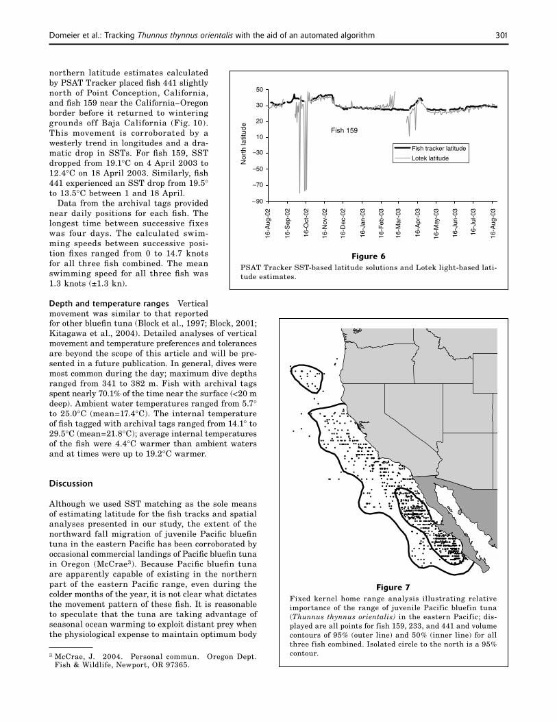
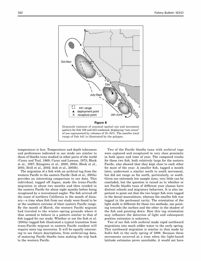
Horizontal movement Tagged bluefin tuna ranged as far north as the California−Oregon border and nearly to the tip of Baja California, Mexico, to the south. Although this distance encompasses 2400 km of coastline, these fish spent the majority of their time in the southern part of the range, best illustrated by a home range analysis of the combined approximately year-long tracks of the three archival tagged bluefin (Fig. 7). Tagged off the northern coast of Baja California, Mexico, these three bluefin moved northward until November, followed by a southward migration to south-central Baja California where they spent the months of January through June (Fig. 8). The two larger archival-tagged fish reached the offshore waters of Oregon before turning south and the smaller fish did not venture north of San Francisco, California. The two larger fish spent much of the winter

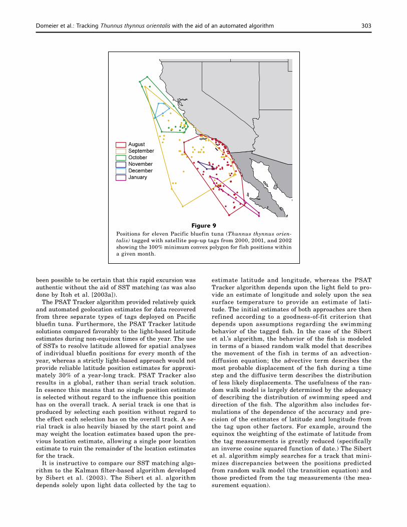
and spring (January–June) in the coastal bight between Punta Eugenia, Mexico, to the north and Cabo San Lazaro, Mexico, to the south, and the smaller fish had a more dispersed spring range north of Punta Euge-nia. In July all three fish began to move to northern Baja, back into the general area where they were originally tagged and where they were subsequently recaptured (Fig. 8). This general pattern of summer−fall move-ment northward followed by a winter migra-tion southward and a winter−spring holding pattern off south-central Baja California was supported by data from fish with PSATs in years 2000 through 2002 (Fig. 9).

Although position data for the months of January through June generally placed the tagged bluefin off southern Baja, two of the three fish tagged with archival tags under-went rapid April excursions to the north be-fore returning to the south (Fig. 10). Fish 159 traveled 2130 km, one way, before return-ing by 1 May; fish 441 made a similar move but did not go as far north (1285 km) and stopped its southward return 480 km north of its original starting point. The extreme


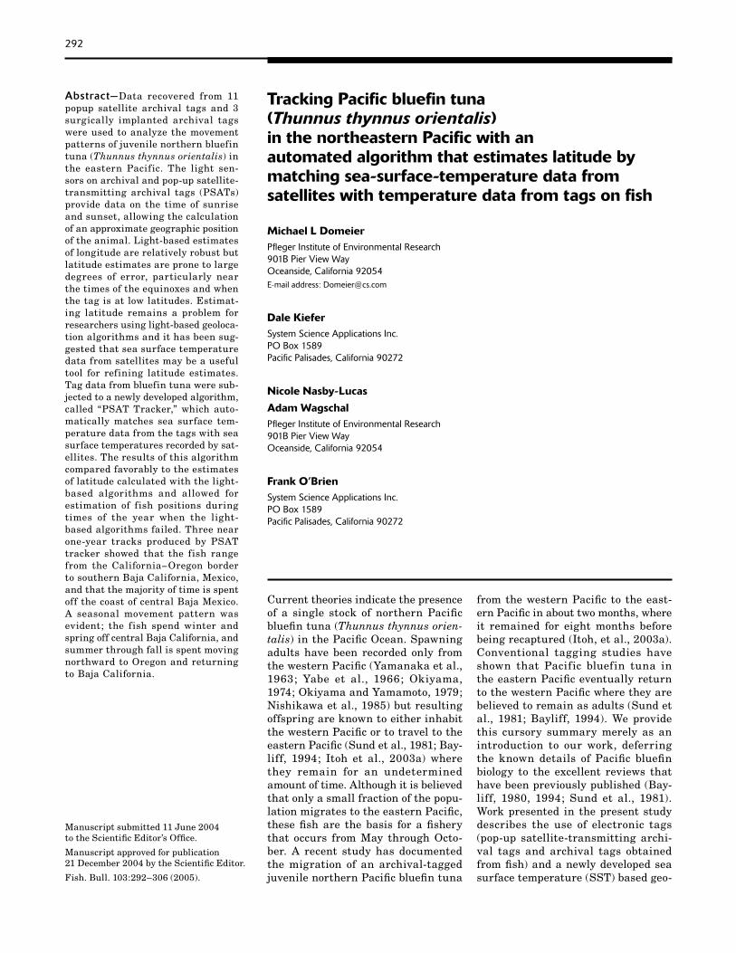
Figure 6PSAT Tracker SST-based latitude solutions and Lotek light-based lati-tude estimates.

50

30

20

10

–30

–50

–70

–90

Fish tracker latitude

Lotek latitude

Nor

th la

titud

e

Fish 159

16-A

ug-0

2

16-S

ep-0

2

16-O

ct-0

2

16-N

ov-0

2

16-D

ec-0

2

16-J

an-0

3

16-F

eb-0

3

16-M

ar-0

3

16-A

pr-0

3

16-M

ay-0

3

16-J

un-0

3

16-J

ul-0

3

16-A

ug-0

3

Figure 7Fixed kernel home range analysis illustrating relative importance of the range of juvenile Pacific bluefin tuna (Thunnus thynnus orientalis) in the eastern Pacific; dis-played are all points for fish 159, 233, and 441 and volume contours of 95% (outer line) and 50% (inner line) for all three fish combined. Isolated circle to the north is a 95% contour.

northern latitude estimates calculated by PSAT Tracker placed fish 441 slightly north of Point Conception, California, and fish 159 near the California−Oregon border before it returned to wintering grounds off Baja California (Fig. 10). This movement is corroborated by a westerly trend in longitudes and a dra-matic drop in SSTs. For fish 159, SST dropped from 19.1°C on 4 April 2003 to 12.4°C on 18 April 2003. Similarly, fish 441 experienced an SST drop from 19.5° to 13.5°C between 1 and 18 April.

Data from the archival tags provided near daily positions for each fish. The longest time between successive fixes was four days. The calculated swim-ming speeds between successive posi-tion fixes ranged from 0 to 14.7 knots for all three fish combined. The mean swimming speed for all three fish was 1.3 knots (±1.3 kn).

Depth and temperature ranges Vertical movement was similar to that reported for other bluefin tuna (Block et al., 1997; Block, 2001; Kitagawa et al., 2004). Detailed analyses of vertical movement and temperature preferences and tolerances are beyond the scope of this article and will be pre-sented in a future publication. In general, dives were most common during the day; maximum dive depths ranged from 341 to 382 m. Fish with archival tags spent nearly 70.1% of the time near the surface (<20 m deep). Ambient water temperatures ranged from 5.7° to 25.0°C (mean=17.4°C). The internal temperature of fish tagged with archival tags ranged from 14.1° to 29.5°C (mean=21.8°C); average internal temperatures of the fish were 4.4°C warmer than ambient waters and at times were up to 19.2°C warmer.

Discussion

Although we used SST matching as the sole means of estimating latitude for the fish tracks and spatial analyses presented in our study, the extent of the northward fall migration of juvenile Pacific bluefin tuna in the eastern Pacific has been corroborated by occasional commercial landings of Pacific bluefin tuna in Oregon (McCrae3). Because Pacific bluefin tuna are apparently capable of existing in the northern part of the eastern Pacific range, even during the colder months of the year, it is not clear what dictates the movement pattern of these fish. It is reasonable to speculate that the tuna are taking advantage of seasonal ocean warming to exploit distant prey when the physiological expense to maintain optimum body

3 McCrae, J. 2004. Personal commun. Oregon Dept. Fish & Wildlife, Newport, OR 97365.


Figure 8Grayscale contours of seasonal spatial use and movement pattern for fish 159 and 233 combined, displaying “core areas” of use represented by volumes of 10−50%. The smaller total range of fish 441 is illustrated by the polygon.

Oct-Nov

July-Sept

Jan-June

XX

441 rangedeployment point

X recapture point

Dec

temperature is less. Temperature and depth tolerances and preferences indicated in our study are similar to those of bluefin tuna studied in other parts of the world (Carey and Teal, 1969; Carey and Lawson, 1973; Block et al., 1997; Kitagawa et al., 2000, 2004; Block et al., 2001; Brill et al., 2002; Itoh et al., 2003b).

The migration of a fish with an archival tag from the western Pacific to the eastern Pacific (Itoh et al., 2003a) provides an interesting comparison to our data. This individual, tagged off Japan, made the trans-Pacific migration in about two months and then resided in the eastern Pacific for about eight months before being recaptured by a recreational angler. The fish arrived off the coast of northern California in the month of Janu-ary—a time when fish from our study were found to be at the southern extreme of their eastern Pacific range. By the month of March, the western Pacific migrant had traveled to the winter−spring grounds where it then seemed to behave in a pattern similar to that of fish tagged for our study. Whether or not the Itoh et al. (2003a) tagged fish illustrated a typical transition from trans-Pacific migrant to eastern Pacific resident will require more tag recoveries. It will be equally interest-ing to see future descriptions, from archival-tag data, of maturing Pacific bluefin tuna making the trip back to the western Pacific.

Two of the Pacific bluefin tuna with archival tags were captured and recaptured in very close proximity in both space and time of year. The computed tracks for these two fish, both relatively large for the eastern Pacific, also showed that they kept close to each other for most of the year. A smaller fish, tagged a month later, underwent a similar north to south movement, but did not range as far north, particularly, or south. Given our extremely low sample sizes, very little can be concluded, but the question is raised as to whether or not Pacific bluefin tuna of different year classes have distinct schools and migratory behaviors. It is also im-portant to point out that the two larger fish were tagged in the dorsal musculature, whereas the smaller fish was tagged in the peritoneal cavity. The orientation of the light stalk is different for these two methods, one point-ing towards the surface and the other in the shadow of the fish and pointing down. How this tag orientation may influence the detection of light and subsequent position estimates is unknown.

Two of our fish with archival made rapid northward migrations into much colder water in the early spring. This northward migration is similar to that made by Itoh’s fish in the early spring of 1998. Because these movements occurred at a time when the light-based latitude estimates prove unreliable, it would not have


Figure 9Positions for eleven Pacific bluefin tuna (Thunnus thynnus orien-talis) tagged with satellite pop-up tags from 2000, 2001, and 2002 showing the 100% minimum convex polygon for fish positions within a given month.

been possible to be certain that this rapid excursion was authentic without the aid of SST matching (as was also done by Itoh et al. [2003a]).

The PSAT Tracker algorithm provided relatively quick and automated geolocation estimates for data recovered from three separate types of tags deployed on Pacific bluefin tuna. Furthermore, the PSAT Tracker latitude solutions compared favorably to the light-based latitude estimates during non-equinox times of the year. The use of SSTs to resolve latitude allowed for spatial analyses of individual bluefin positions for every month of the year, whereas a strictly light-based approach would not provide reliable latitude position estimates for approxi-mately 30% of a year-long track. PSAT Tracker also results in a global, rather than serial track solution. In essence this means that no single position estimate is selected without regard to the influence this position has on the overall track. A serial track is one that is produced by selecting each position without regard to the effect each selection has on the overall track. A se-rial track is also heavily biased by the start point and may weight the location estimates based upon the pre-vious location estimate, allowing a single poor location estimate to ruin the remainder of the location estimates for the track.

It is instructive to compare our SST matching algo-rithm to the Kalman filter-based algorithm developed by Sibert et al. (2003). The Sibert et al. algorithm depends solely upon light data collected by the tag to

estimate latitude and longitude, whereas the PSAT Tracker algorithm depends upon the light field to pro-vide an estimate of longitude and solely upon the sea surface temperature to provide an estimate of lati-tude. The initial estimates of both approaches are then refined according to a goodness-of-fit criterion that depends upon assumptions regarding the swimming behavior of the tagged fish. In the case of the Sibert et al.’s algorithm, the behavior of the fish is modeled in terms of a biased random walk model that describes the movement of the fish in terms of an advection- diffusion equation; the advective term describes the most probable displacement of the fish during a time step and the diffusive term describes the distribution of less likely displacements. The usefulness of the ran-dom walk model is largely determined by the adequacy of describing the distribution of swimming speed and direction of the fish. The algorithm also includes for-mulations of the dependence of the accuracy and pre-cision of the estimates of latitude and longitude from the tag upon other factors. For example, around the equinox the weighting of the estimate of latitude from the tag measurements is greatly reduced (specifically an inverse cosine squared function of date.) The Sibert et al. algorithm simply searches for a track that mini-mizes discrepancies between the positions predicted from random walk model (the transition equation) and those predicted from the tag measurements (the mea-surement equation).


Figure 10Track showing northward excursions of fish 159 (track extending to 38°) and 441 (track extending to 34.5°) between 1 April and 10 May 2003. Displayed SST imagery is a composite for the month of April showing a 7°C temperature gradient.

PSAT Tracker is similar to the Sibert et al. algorithm in that it invokes a model of fish behavior; there is a simple constraint on the maximum distance that a fish can swim during a time step, and shorter tracks that require lesser expenditures of energy by the fish are favored. Like the Sibert et al. algorithm, the PSAT Tracker also incorporates candidate points that are not limited to the initial light-based estimate of longitude but includes adjacent longitudes based upon the user’s assessment of the accuracy of the initial estimate. Fi-nally, both the Sibert et al. and the PSAT Tracker al-gorithms yield a solution that provides a best fit to the time series of satellite (in the case of PSAT Tracker) and tag measurements to the model of fish behavior.

Unfortunately, it is difficult to make a general assess-ment of the accuracy of either approach. In the case of the PSAT Tracker algorithm, the accuracy of the track will decrease in the absence of a north−south tempera-ture gradient. We have not found a means of quantita-tively determining the accuracy of PSAT Tracker cal-culations. However, the quality of the fit between pixel values of temperature from imagery and tag values for positions along the track is calculated as a χ2 value. In the case of the Sibert et al. algorithm, the accuracy of the track will decrease during the period of the equinox when the latitudinal errors of the light-based estimates

are extremely large. Our data indicate that this period can be as long as two months surrounding each equinox (skewed towards winter). At such times the estimates of position derived by the Sibert et al. algorithm depend largely on the random walk model of fish movement, which provides only a generic description of movement. Although the algorithm provides values for the mean square errors of bias and randomness for the tag es-timates of latitude and longitude, these values are not true values for error of predicting location; rather they represent of the discrepancy between the estimates of position by the random walk model, the formulation of the latitude estimation error, and the tag measure-ments. Additionally, the Sibert et al. algorithm does not exclude the possibility of placing a fish on land.

The PSAT Tracker worked well for this study because of the strong north-to-south temperature gradient that is presented in the northeastern Pacific. Studies conducted in regions with poor temperature gradients will continue to rely on light-based latitude estimates and approaches like the Sibert et al. algorithm. Further development of PSAT Tracker, or other SST-based geolocation al-gorithms, should explore a means of using light-based latitude positions in combination with SST matching when light data are reliable, but excluding light-derived latitude positions when they are unreliable.


Acknowledgments

This study was made possible through the support of the George T. Pfleger Foundation and the Offield Family Foundation. We thank those who helped us capture the fish in our study: Tom Pfleger, Tom Fullam, Tom Roth-erie, Greg Stutzer and Chugey Sepulveda. Archival tags were recovered with the assistance of the Inter-American Tropical Tuna Commission.

Literature cited

Bayliff, W. H. 1980. Synopsis of biological data on the northern bluefin

tuna, Thunnus thynnus (Linnaeus, 1758), in the Pa- cific Ocean. Inter-Am. Trop. Tuna Comm. Spec. Rep. 2: 261−293.

1994. A review of the biology and fisheries for northern bluefin tuna, Thunnus thynnus, in the Pacific Ocean. FAO Fish. Tech. Paper 336, part 2:244−295.

Block, B. A., H. Dewar, S. B. Blackwell, T. D. Williams, E. D. Prince, A. Boustany, C. F. Farwell, D. J. Dau, and A. Seitz.

2001. Archival and pop-up satellite tagging of Atlantic bluefin tuna. In Electronic tagging and tracking in marine fishes (J. R. Sibert and J. L. Nielsen, eds.), p. 65−68. Kluwer Academic Publs, The Netherlands.

Block, B.A., H. Dewar, T. Williams, E. Prince, C. Farwell, and D. Fudge.

1997. Archival and pop up satellite tagging of Atlantic bluefin tuna, Thunnus thynnus. In Proceedings of the 48th annual tuna conference, p. 10. Inter-Am. Trop. Tuna Comm., Lake Arrowhead, CA.

1998. Archival tagging of Atlantic bluefin tuna (Thunnus thynnus thynnus). MTS Journal 32:37−46.

Bowditch, N. 1995. The American practical navigator: an epitome of

navigation. Originally by Nathaniel Bowdich (1802), Publ. 9., 873 p. Defense Mapping Agency Hydrographic/Topographic Center, Bethesda, MD.

Brill, R., M. Lutcavage, G. Metzger, P. Bushnell, M. Arendt, J. Lucy, C. Watson, and D. Foley.

2002. Horizontal and vertical movements of juvenile blue-fin tuna (Thunnus thynnus), in relation to oceanographic conditions of the western North Atlantic, determined with ultrasonic telemetry. Fish. Bull. 100:155−167.

Carey, F. G., and K. D. Lawson. 1973. Temperature regulation in free-swimming bluefin

tuna. Comp. Biochem. Physiol. 44a:375−395.Carey, F. G., and J. M. Teal.

1969. Regulation of body temperature by the bluefin tuna. Comp. Biochem. Physiol. 28:205−213.

Delong, R. I., B. S. Stewart, and R. D. Hill. 1992. Documenting migrations of northern elephant seals

using day length. Mar. Mamm. Sci. 8:155−159.Hill, R.

1994. Theory of geolocation by light levels. In Ele- phant seals: population ecology, behavior, and physiology (B. J. LeBoeuf and R. M. Laws, eds.), p. 227− 236. Univ. California Press, Berkeley, CA.

Hill, R. D., and M. J. Braun. 2001. Geolocation by light-level. The next step: lati-

tude. In Electronic tagging and tracking in marine fish-

erie (J. Sibert and J. Nielsen, eds.), p. 315−330. Kluwer Academic Press, Dordrecht, The Netherlands.

Itoh, T., S. Tsuji and A. Nitta. 2003a. Migration patterns of young Pacif ic bluefin

tuna (Thunnus orientalis) determined with archival tags. Fish. Bull. 101:514−534.

2003b. Swimming depth, ambient water temperature preference, and feeding frequency of young Pacific blue-fin tuna (Thunnus thynnus orientalis) determined with archival tags. Fish. Bull. 101:535−544.

Kitagawa, T., S. Kimura, H. Nakata, and H. Yamada. 2004. Diving behavior of immature, feeding Pacific bluefin

tuna (Thunnus thynnus orientalis) in relation to season and area: the East China Sea and the Kuroshio-Oyashio transition region. Fish. Oceanogr. 13(3):161−180.

Kitagawa, T., H. Nakata, S. Kimura, T. Itoh, S. Tsuji, and A. Nitta.

2000. Effect of ambient temperature on the vertical distribution and movement of Pacific bluefin tuna Thunnus thynnus orientalis. Mar. Ecol. Prog. Ser. 206:251−260.

Metcalfe, J. D. 2001. Summary report of a workshop on daylight measure-

ments for geolocation in animal telemetry. In Electronic tagging and tracking in marine fisheries (J. Sibert and J. Nielsen, eds.), p. 331−342. Kluwer Academic Press, Dordrecht, The Netherlands.

Musyl, M. K., R. W. Brill, D. S. Curran, J. S. Gunn, J. R. Hartog, R. D. Hill, D. W. Welch, J. P. Eveson, C. H. Boggs, and R. E. Brainard.

2001. Ability of archival tags to provide estimates of geo-graphical position based on light intensity. In Electronic tagging and tracking in marine fisheries (J. Sibert and J. Nielsen, eds), p. 343−368. Kluwer Academic Press, Dordrecht, The Netherlands.

Musyl, M. K., R. W. Brill, C. H. Boggs, D. S. Curran, T. K. Kazama, and M. P. Seki.

2003. Vertical movements of bigeye tuna (Thunnus obesus) associated with islands, buoys, and seamounts near the main Hawaiian islands from archival tagging data. Fish. Oceanogr. 12:152−169.

Nishikawa, Y., M. Honma, S. Ueyanagi, and S. Kikawa. 1985. Average distribution of larvae of oceanic species

of scombrid fishes, 1956−1981. Nat. Res. Institute of Far Seas Fisheries, Shimizu. 12:99.

Okiyama, M. 1974. Occurrence of the postlarvae of bluefin tuna,

Thunnus thynnus, in the Japan Sea. Japan Sea Reg. Fish. Res. Lab. Bull. 25:89−97.

Okiyama, M., and G. Yamamoto. 1979. Successful spawning of some holepipelagic fishes

in the Sea of Japan and zoogeographical implications. In Proceedings of the seventh Japan-Soviet joint sym-posium on aquaculture, p. 223−233. Tokai Univ. Press, Tokyo, Japan.

Rodgers, A. R., and A. P. Carr. 1998. HRE: the home range extension for ArcView. Us-

er’s manual, 27 p. Centre for Northern Forest Ecosys-tem Research, Ontario Ministry of Natural Resources, Thunder Bay, Ontario, Canada.

Schaefer, K. M., and D. W. Fuller. 2002. Movements, behavior, and habitat selection of

bigeye tuna (Thunnus obesus) in the eastern equato-rial Pacific, ascertained through archival tags. Fish. Bull. 100:765−788.


Sibert, J. R., M. K. Musyl, and R. W. Brill. 2003. Horizontal movements of bigeye tuna (Thunnus

obesus) near Hawaii determined by Kalman filter analyis of archival tag data. Fish. Oceanogr. 12(3):141−151.

Sobel, D. 1995. Longitude: the true story of a lone genius who

solved the greatest scientific problem of his time, 184 p. Penguin Books, New York, NY.

Sund, P. N., M. Blackburn, and F. Williams. 1981. Tunas and their environment in the Pacific Ocean: a

review. Oceanogr. Mar. Biol. Ann. Rev. 19:443−512.Welch, D. W., and J. P. Eveson.

1999. An assessment of light-based geoposition esti-mates from archival tags. Can. J. Aquat. Sci. 56:13171− 1327.

2001. Recent progress in estimating geoposition using daylight. In Electronic tagging and tracking

in marine fisheries (Sibert and J. Nielsen, eds.), p. 3693−83. Kluwer Academic Press, Dordrecht, The Netherlands.

Wilson, R. P., J. J. Ducamp, W. G. Rees, B. M. Culik, and K. Neikamp. 1992. Estimation of location: global coverage using light

intensity. In Wildlife telemetry: remote monitoring and tracking of animals (I. G. Priede and S.M. Swift, eds.) p. 131−134. Ellis Horwood, New York, NY.

Yabe, H., S. Ueyanagi, and H. Watanabe. 1966. Studies on the early life history of bluefin tuna

Thunnus thynnus and on the larvae of the southern bluefin tuna T. maccoyii. Rep. Nankai Reg. Fish. Res. Lab. 23:95−129.

Yamanaka, H., and staff (sic). 1963. Synopsis of biological data on kuromaguro Thun-

nus orientalis (Temminck and Schlegel) 1942 (Pacific Ocean). FAO Fish Rep, 6(2):180−217.

art & equations are linked preflight goodfishbull.noaa.gov/1032/domeier.pdf · art &...

Documents