art-3a10.1007-2fs00603-009-0054-0

ORIGINAL PAPER

The Planar Shape of Rock Joints

Lianyang Zhang Æ Herbert H. Einstein

Received: 26 September 2008 / Accepted: 16 May 2009 / Published online: 3 June 2009

� Springer-Verlag 2009

Abstract Knowing the planar shape of discontinuities is

important when characterizing discontinuities in a rock

mass. However, the real discontinuity shape is rarely

known, since the rock mass is usually inaccessible in three

dimensions. Information on discontinuity shape is limited

and often open to more than one interpretation. This paper

discusses the planar shape of rock joints, the most common

discontinuities in rock. First, a brief literature review about

the shape of joints is presented, including some information

on joint-surface morphology, inferences from observed

trace lengths on different sampling planes, information

based on experimental studies, and joint shapes assumed by

different researchers. This review shows that joints not

affected by adjacent geological structures such as bedding

boundaries or pre-existing fractures tend to be elliptical (or

approximately circular but rarely). Joints affected by or

intersecting such geological structures tend to be rectan-

gular. Then, using the general stereological relationship

between trace length distributions and joint size distribu-

tions developed by Zhang et al. (Geotechnique 52(6):419–

433, 2002) for elliptical joints, the effect of sampling plane

orientation on trace lengths is investigated. This study

explains why the average trace lengths of non-equidimen-

sional (elliptical or similar polygonal) joints on two sam-

pling planes can be about equal and thus the conclusion

that rock joints are equidimensional (circular) drawn from

the fact that the average trace lengths on two sampling

planes are approximately equal can be wrong. Finally,

methods for characterizing the shape and size of joints

(elliptical or rectangular) from trace length data are rec-

ommended, and the appropriateness of using elliptical joint

shapes to represent polygonal, especially rectangular, joints

is discussed.

Keywords Rock discontinuity � Rock fracture �Rock joint � Planar shape � Geology

1 Introduction

Research results have shown that the planar shape of

discontinuities has a profound effect on the connectivity

of discontinuities and on the strength, deformability and

permeability of rock masses (e.g., Petit et al. 1994;

Dershowitz 1998; Zhang 2005). Consequently, it is

important to know the planar shape of discontinuities when

characterizing them in a rock mass. However, the real

discontinuity shape at a site is rarely known, since a rock

mass is usually inaccessible in three dimensions. Infor-

mation on discontinuity shape is limited and often open to

more than one interpretation (Warburton 1980a; Wathugala

1991). This paper discusses the planar shape of rock joints

(or fractures),1 the most common discontinuities in rock.

Joints include tension joints involving displacement per-

pendicular to the fracture walls and shear joints involving

some shear displacement of the fracture walls that remains

‘‘invisible’’ at the scale of observation (ISRM 1978; Mandl

2005). Although some researchers such as Pollard and

Aydin (1988) have reservations about the definition of

L. Zhang (&)

Department of Civil Engineering and Engineering Mechanics,

University of Arizona, Tucson, AZ, USA

e-mail: [email protected]

H. H. Einstein

Department of Civil and Environmental Engineering,

Massachusetts Institute of Technology, Cambridge, MA, USA

1 The terms joint and fracture will be used interchangeably as is often

the case in the engineering literature.

123

Rock Mech Rock Eng (2010) 43:55–68

DOI 10.1007/s00603-009-0054-0

shear joints, this paper adopts the most widely accepted

definition of joints as described above. Dershowitz and

Einstein (1988) stated: ‘‘Shape of joint boundaries can be

polygonal, circular, elliptical or irregular. Joints can be

planar or non-planar in space and shape should consider

this fact also. Since joints are often planar, it is simpler to

associate ‘shape’ with the two-dimensional appearance

and treat non-planarity separately.’’ This paper mainly

discusses the shape of planar joints, but makes some

comments on joint surface morphology.

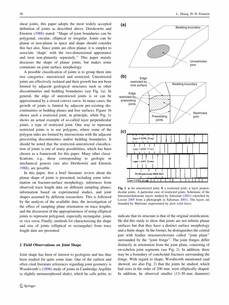
A possible classification of joints is to group them into

two categories: unrestricted and restricted. Unrestricted

joints are effectively isolated and their growth has not been

limited by adjacent geological structures such as other

discontinuities and bedding boundaries (see Fig. 1a). In

general, the edge of unrestricted joints is or can be

approximated by a closed convex curve. In many cases, the

growth of joints is limited by adjacent pre-existing dis-

continuities or bedding planes and free surfaces. Figure 1b

shows such a restricted joint, in principle, while Fig. 1c

shows an actual example of so-called layer perpendicular

joints, a type of restricted joint. One way to represent

restricted joints is to use polygons, where some of the

polygon sides are formed by intersections with the adjacent

preexisting discontinuities and/or bedding boundaries. It

should be noted that the restricted–unrestricted classifica-

tion of joints is one of many possibilities, which has been

chosen as a framework for this paper. Many other classi-

fications, e.g., those corresponding to geologic or

mechanical genesis (see also Dershowitz and Einstein

1988), are possible.

In this paper, first a brief literature review about the

planar shape of joints is presented, including some infor-

mation on fracture-surface morphology, inferences from

observed trace length data on different sampling planes,

information based on experimental studies, and joint

shapes assumed by different researchers. This is followed

by the analysis of the available data, the investigation of

the effect of sampling plane orientation on trace lengths,

and the discussion of the appropriateness of using elliptical

joints to represent polygonal, especially rectangular, joints

or vice versa. Finally, methods for characterizing the shape

and size of joints (elliptical or rectangular) from trace

length data are presented.

2 Field Observations on Joint Shape

Joint shape has been of interest to geologists and has thus

been studied for quite some time. One of the earliest and

often cited literature references regarding joint geometry is

Woodworth’s (1896) study of joints in Cambridge Argillite

(a slightly metamorphosed shale), which he calls pelite, to

indicate that its structure is that of the original stratification.

He did this study to show that joints are not infinite planar

surfaces but that they have a distinct surface morphology

and a finite shape. In the former, he distinguishes the central

part with feather structures/texture called ‘‘joint plane’’

surrounded by the ‘‘joint fringe’’. The joint fringes differ

distinctly in orientation from the joint plane, consisting of

en-echelon joint segments (see Fig. 2). In addition, there

may be a boundary of conchoidal fractures surrounding the

fringe. With regard to shape, Woodworth mentioned (and

showed, see also Fig. 2) that the joints he studied, which

had sizes in the order of 200 mm, were elliptically shaped.

In addition, he observed smaller (13–50 mm diameter)

Bedding boundary

Bedding boundary

Edgerestricted by

preexistingjoints

Unrestrictedjoint

RestrictedjointPreexisting

joints

(a)

(b)

(c)

Edgerestricted byrock surface

Fig. 1 a An unrestricted joint; b a restricted joint; c layer perpen-

dicular joints. A particular case of restricted joints. Schematic of the

limestone/dolostone layers studied by Saltzman (2001) (sketched by

Locsin 2005 from a photograph in Saltzman 2001). The layers are

bounded by Marlsone (represented by dark solid lines)

56 L. Zhang, H. H. Einstein

123

so-called discoid joints of circular/elliptical shape. Wood-

worth (1896) also mentions that feather surface morphology

can also be observed in a variety of igneous rocks. Hodgson

(1961) refined Woodworth’s information by distinguishing

systematic and non-systematic joints on the basis of surface

morphology and mentioned briefly that ‘‘most systematic

joints are elliptical, ranging from very elongated to mod-

erately elongated in the direction of the plane axis’’. He then

went on to say that surface structure is rarely radial (plu-

mose structures emanating from a point and producing a

circular joint). Hodgson (1961) finally commented on cross-

joints, one of the non-systematic joints, and stated that they

extend between systematic joints and often terminate

against other non-systematic or systematic joints. One can

infer from this, but Hodgson did not say so, that such cross

joints will have a rectangular shape.

Another set of detailed observations on fracture surfaces

and shapes are those by Bankwitz (1965). Figure 3 shows

the fracture morphology consisting of plumose features in

the center part (Hauptkluft after Bankwitz), radial features

(Radialklufte after Bankwitz) and stepped boundary fea-

tures (Randklufte after Bankwitz) (This subdivision is to

some extent similar to that by Woodworth—the Hauptkluft

corresponds to Woodworth’s joint plane, while the

‘‘Radial’’—and ‘‘Randklufte’’ together correspond to

Woodworth’s fringe.). Since the morphology mentioned

here is similar to Woodworth, one of the main interests of

Bankwitz in this and the following papers (Bankwitz 1966,

1978; Bankwitz and Bankwitz 1984) is the fact that frac-

tures are not planar but three-dimensional features. He

shows a systematic sketch of fracture development in his

next paper (Bankwitz 1966) which is reproduced in Fig. 4.

The fact that fractures are or can be three-dimensional has

to be kept in mind; in other words, the assumption of

planarity is a simplification, although an acceptable one in

the context of this paper. Another reason why this is

mentioned is that the features shown in Fig. 3 are charac-

teristic of most but by no means all, tensile fractures. For

instance cooling (columnar) joints rarely show these fea-

tures, while sheet joints often but not always do. This and

the difference to shear-related fractures has been discussed

not only by Dershowitz and Einstein (1988) but also by

many others (e.g., Cloos 1955; Einstein and Dershowitz

1990; Einstein and Bobet 2004; Gross et al. 1997; Hoek

1968; Horii and Nemat-Nasser 1986; Lajtai 1969; Price

1966; Riedel 1929; Saltzman 2001; Sheldon 1912).

Fig. 2 Drawings of surface markings and profiles of joints in

Cambridge Argillite: A the entire joint surface (a center, b border,

c cross fractures, d edge of joint plane = inner margin of fringe,

e axis of feather fractures); B joint fringe region (b) with echelon joint

segments (c) [from Woodworth 1896 Plate 1, Fig. 10 (A in this

figure), Fig. 5 (B in this figure)]

Fig. 3 Joint with plumose (1) and ring structures (2), radial (3) and

boundary joints (4), which lead over to en-echelon jointing. The

plumose structures are only indicated in the upper part. Griffelschie-

fer (schist) from the schist quarries at the Trebenkopf, west of

Oberwirbach (Sheet Bad Blankenburg). This figure is Fig. 5 in

Bankwitz (1965). The legend has been translated from the German

original. The numbers in parentheses and the numbers in the figure

which identify the various features have been added by the authors of

this paper

The Planar Shape of Rock Joints 57

123

It is important to note at this point that fracture (joint)

genesis has been studied intensively by many researchers,

and what is quoted above is only a selection. Readers

interested in more details are referred to Ameen (1995) in

which much of the relevant (up to that time) literature is

summarized.

After these initial comments about surface morphology,

we will now concentrate on Bankwitz’s (1965, 1966)

comments on shape. Bankwitz (1965) did these studies in

the ‘‘Thuringer Schiefergebirge’’ with a variety of meta-

morphic lithologies (different schists, quartzite) and also

considering igneous intrusions (diabase, granite). His

statement about fracture shape is quoted here (translated

from German):

‘‘The fractures in an outcrop are normally a series of

either elliptical (ideally circular) [fractures] and have

a natural termination in the rock, or—and this holds

for the greater number—they end at other fractures,

bedding or schistocity surfaces, etc. The latter have,

therefore, linear boundaries. To the problem of frac-

ture genesis, the first group is very important.’’

These ‘‘classic’’ early studies on joint shape (Wood-

worth 1896; Bankwitz 1965 and later) therefore indicate

that one often sees elliptical shapes, where elongated

ellipses may be caused by boundary layers. In addition,

rectangular shapes can also be observed, particularly if

bounded by existing joints.

More recent studies, in which elliptical joint shapes

were reported, are those by Kulander et al. (1979), Bahat

(1988), Petit et al. (1994), Weinberger (2001), Bahat et al.

(2003), and Savalli and Engelder (2005).

Weinberger (2001) analyzed the surface morphology of

joints in the dolomite layers of the Judea Group, Israel in

order to study the role played by spherical cavity-shaped

flaws during nucleation and growth of joints. He found that

joints typically show two forms of growth, depending on

the abundance and spatial distribution of cavities within the

layers. In layers with many cavities, joints preferably ini-

tiate at critical cavities, propagate vertically toward bed-

ding interfaces and horizontally toward adjacent joints, and

form elliptical fractures. In layers free of cavities, joints

initiate at bedding interfaces, commonly propagate down-

ward toward the layer base and adjacent joints, and form

semi-elliptical fractures. In both cases, the joint propaga-

tion is impeded by the bedding interfaces between the

dolomite layers.

Bahat et al. (2003) studied the joints in the Borsov

granite based on analyses of joint-surface morphology of

ten exposed joints in a quarry. The study area is located in

the South Bohemian Pluton. The results show that the

joints in the Borsov granite have a mirror plane (a smooth

crack surface that contains the initial and critical flaws, the

striae, and the undulations), which is either (approxi-

mately) circular or elliptical. For joints with exposed

boundaries, the mirror planes deviate from circularity into

various ellipses (see Fig. 5).

Fig. 4 Development of ‘‘radial

joints’’ according to Bankwitz

(1966)

Fig. 5 Elliptical propagation of fracture confined by two subhori-

zontal boundaries (above and below) (from Bahat et al. 2003)


123

Savalli and Engelder (2005) studied the mechanisms

controlling rupture shape during the growth of joints in

layered clastic rocks based on field observations of exposed

joints. In layered rocks, a rupture can initiate either from

the interior of a bed or from the bed boundary, which is

similar to the conclusion drawn by Weinberger (2001)

discussed above. Maps of tip line profiles during early joint

growth (before intersecting the bed boundary) delineate

(approximately) circular and elliptical rupture shapes. For

homogeneous and isotropic rock, the velocity of the crack

tip line is equal in all directions at the onset of rupture and

the rupture shape during early joint growth will be simply

circular. Since natural rock is usually inhomogeneous and

anisotropic, the rupture shape during early joint growth will

not be (perfectly) circular. After the joint intersects the bed

boundary(ies), the crack tip line will split into two dis-

continuous moving segments and the two separate tip lines

will move synchronously away from each other, forming

(approximately) elliptical or rectangular rupture shape (see

Fig. 6).

The photos in Fig. 7 which have been taken in the

Grimsel area in Switzerland show several things: the rock

mass is granitic and characterized by classic sheet join-

ting with joint spacing ranging from the scale of many

meters to centimeters (Fig. 7a). The photos also show

that there are both restricted (mostly rectangular) and

unrestricted (elliptical) joints. The latter are particularly

well exposed in the lower left of Fig. 7a and in the lower

part of Fig. 7b. Also note in both photos the joint mor-

phologic features such as the plumose features mentioned

earlier.

A study of particular interest regarding the differentia-

tion between elliptical (possibly circular) and rectangular

joints is that by Petit et al. (1994). They studied joints in

(b)

(a)

Bed boundary

Crack tip lines

Simple rupture shapes

Closed rupture (t1)

Detached rupture Open rupture (t2)

Initiation point

Stress concentrator

Bed boundary

Inclusion hackles/ Plumose lines

Hesitation/arrest lines (the rupture at t1)

Plume axis

Fig. 6 a Natural features on

joint surfaces. Joints initiate at

and propagate away from a

stress concentration point.

Plumes (i.e., barbs, inclusion

hackles, striae, plume lines)

diverge from the initiation point

in the propagation direction.

Arrest lines form at right angles

to plumes where the crack tip

hesitated or arrested.

b Interpretive features on joint

surfaces. Crack tip lines are the

dashed curves drawn

perpendicularly to plume traces.

Rupture shapes coincide with

the trace of the crack tip line at

three stages of rupture growth,

ti (i = 1, 2, 3) (from Savalli and

Engelder 2005)

Fig. 7 Exposed rock fractures in the Grimsel area in Switzerland

(Photo by H. Einstein)


123

the Permian sandstones of the Lodeve basin in France,

which consist of relatively massive pelites and isolated

sandstone layers within the pelite. As will be seen later, the

joint characteristics in pelite and sandstone are quite dif-

ferent. Before summarizing what Petit et al. observed, it is

interesting to note that they initiated this field study,

because they were dissatisfied with mostly mathematically

oriented preceding studies leading to randomly distributed

(circular?) disks. Petit et al. concentrated on Mode I frac-

tures. In the pelites, a steeply dipping set of joints was

observed, specifically the vertical extent H and the hori-

zontal extent L, which they backfigured from joint traces

visible on 10–15� inclined outcrops (exposures). Statistics

based on 55 measurements gave Lmean = 5.1 m,

Hmean = 2.7 m both showing lognormal distribution. This

results in an aspect ratio of L/H = 1.9. Petit et al. also

explicitly observed several isolated ellipses (with plumose

surface features, etc.) of similar aspect ratio (2.0). They

conclude that excluding some circular and some elongated

features, one can assume a general elliptical form for

fractures in the pelites. In addition, they observed abutting

fractures (geometry limited by existing fractures), which

are apparently rectangular with higher L/H. In the isolated

sandstone layers, however, the result was quite different.

These measurements were made in two beds where the bed

thickness corresponds to joint height H, while joint trace

length L was measured as such. The results were as

follows: L/H [ 5.0 and L/H [ 4.0 and definitely of

rectangular form.

Locsin (2005) in the context of developing models for

‘‘layer perpendicular’’ joints studied a number of cases,

mostly in sedimentary rocks. Layer perpendicular joints

occur in rocks where the layers differ in stiffness and

where, as a consequence, jointing occurs mostly in the

stiffer layer. The cases studied were those reported by

Becker and Gross (1996) and by Saltzman (2001) on the

limestone/dolostone Gerofit formation in Israel, by Gross

et al. (1997) on six interbedded chalk/chert layer near

Beersheba (Israel) and by Baudo (2001) on sandstones and

shales of the Upper Canadaway formation exposed along

Cattaraugus Creek in Southwestern New York State. The

vertical heights of the joint traces in all these cases are

equal to the thicknesses of the jointing layers, i.e., for the

limestone/dolostone Gerofit formation in Becker and Gross

(1996) and Saltzman (2001) between 0.12 and 0.52 m, for

the chalk in Gross et al. (1997) between 0.17 and 0.63 m,

and for the sandstone/schistose layer in Baudo (2001)

0.09 m while for the three other sandstone layers in Baudo

(2001) this is 0.1 m. In all cases, the beds/layers are flatly

dipping or horizontal. While no or only very limited

measurements of horizontal trace lengths have been

reported, one can infer from the information on bed

thickness (equal to joint height), and bed orientation and

geologic setting that the joints are essentially rectangular

with large aspect ratios. These are again all cases where

there is a strong boundary effect in that the jointing layer is

usually stiffer than the bounding non-jointing layer.

Many other articles and reports have appeared in the last

three decades discussing possible shapes of joints based on

in-situ trace length data (Figure 8 shows the strike and dip

traces of a joint.):

1. Robertson (1970), after analyzing nearly 9,000 traces

from the De Beer mine, South Africa, concluded that

the strike trace length and the dip trace length of joints

have about the same distribution, possibly implying

joints to be equidimensional (circular).

2. Bridges (1976) stated that ‘‘there is good evidence for’’

individual joints to be taken to have a rectangular

(elongated) shape, especially for joints in anisotropic

rock. However, no specific data can be found in the

original paper to support this statement.

Strike

Dip

Joint

Samplingplane 1

Joint

Samplingplane 2

Striketrace

Diptrace

(b)

(a)

Fig. 8 a Strike and dip of a joint, and b Strike and dip traces


123

3. Barton (1977) presented a geotechnical analysis of

rock structure and fabric at the C.S.A. Mine, Cobar,

NSW, Australia. The country rock within the mine

area is overwhelmingly composed of chloritic and

quartzitic siltstone to slaty claystone. Based on obser-

vations of trace lengths of joints visible on wall

photographs of cross cuts, Barton (1977) concluded

that joints are approximately equidimensional.

4. Einstein et al. (1979) investigated joints at a site in

southern Connecticut. The country rock at this site is

the Monson gneiss, a thinly banded rock with

feldspathic and biotitic layers. There are two major

joint sets at this site. Set 1 dips steeply to the southeast

and set 2 is nearly horizontal. Trace lengths of joints

were measured on both the horizontal and vertical

surfaces of excavations. The results indicate that joints

are non-equidimensional (see Table 1).

From all the above, one can infer that joints formed in

extension have elongated shapes where these shapes can be

either elliptical or rectangular (occasionally other polygo-

nal shapes). Circular disks can occur but do so rarely, and

they can be considered special cases of ellipses.

3 Joint Shape Based on Experimental Studies

Researchers have also studied the shape of joints experi-

mentally. Daneshy (1973) experimentally investigated the

shape of hydraulically induced fractures in hydrostone and

limestone by studying fracture characteristics: facial fea-

tures, hackle marks, and rib marks. The experiments were

conducted on rectangular blocks of 152 mm 9 152 mm 9

254 mm. A borehole of 254 mm long and 7.95 mm in

diameter was drilled from the center of the top square to

the center of the bottom square. Two steel tubings of equal

length were then cemented at the top and the bottom of the

borehole. Different heights of the open-hole part were

obtained by changing the lengths of the casings. Fractures

were then induced by injecting fluid into the borehole. The

results indicate that hydraulic fractures extending from a

point source (very short open-hole part) propagate radially,

with their edge having a circular shape. The fractures

extending from a line source (long open-hole part), how-

ever, propagate on a hyperbolic path, with their edge

having an elliptical shape. As the elliptical fracture prop-

agates further, the shape of the fracture tends more and

more toward being circular.

Moriya et al. (2006) examined the propagation of frac-

tures at the Bernburg salt mine by analyzing hydraulically

induced acoustic emissions (AE). The results show that the

AE source locations are distributed as an ellipse and the

principal direction of the source distribution changes

according to the change of the principal stress direction,

indicating that the shape of the fracture is elliptical (see

Fig. 9).

Table 1 Mean of strike trace lengths and mean of dip trace lengths of

two joint sets (from Einstein et al. 1979)

Joint set # Mean of strike

trace lengths (foot)

Mean of dip

trace lengths (foot)

1 28.3 16.1

2 25.2 21.1

Strike direction (m)

Strike direction (m)

Dip

dire

ctio

n (m

)D

ip d

irect

ion

(m)

0.5 m

0.5 m

Aspect ratio = 1.15

Max. stress direction on plane

Aspect ratio = 1.18

Max. stress direction on plane

Fracturing tests Re-fracturing tests Points where fracturing well crosses source distribution plane

(a)

(b)

Fig. 9 Acoustic emission (AE) source locations at a fracturing point

FS2, and b fracturing point FS5 (from Moriya et al. 2006)


123

4 Assumptions About the Joint Shape by Different

Researchers

Researchers have assumed different joint shapes for dif-

ferent research and application purposes. Due to the

mathematical convenience, many investigators assume that

joints are thin circular disks randomly located in space

(Baecher et al. 1977; Warburton 1980a; Chan 1986;

Villaescusa and Brown 1990; Kulatilake et al. 1993; Song

and Lee 2001; Song 2006). Baecher later extended his

model to also include elliptical joints (Einstein et al. 1979).

With circular joints, the trace patterns in differently

oriented sampling planes will be the same. In practice,

however, the trace patterns may vary with the orientation

of sampling planes (Warburton 1980b). Therefore,

Warburton (1980b) assumed that joints in a set are para-

llelograms of various sizes. Kulatilake et al. (1990) not

only considered joints as circular disks but also as rectan-

gles, squares, right triangles, parallelograms, rhombuses,

and oblique triangles in their study of the effect of joint

orientation, joint size, and joint shape on the statistical

distribution of the orientation.

Dershowitz et al. (1993) used polygons to represent

joints in his discrete fracture code. The polygons are

formed by inscribing a polygon in an ellipse (see Fig. 10).

Ivanova (1995, 1998) and Meyer (1999) also used polygons

to represent joints in their discrete fracture code. It is noted

that polygons can be used to effectively represent elliptical

joints when the number of polygon sides is large (Der-

showitz et al. 1993) or vice versa.

Zhang et al. (2002) considered joints to be ellipses and

derived the general stereological relationship between

trace length distribution and joint size (represented by the

major axis length of the ellipse) distribution. Based on the

general stereological relationship, they investigated the

effect of sampling plane orientation on trace lengths and

proposed a method for inferring the size distribution of

elliptical joints from trace length sampling on different

sampling planes.

5 Analysis of Existing Information on Joint Shape

As discussed above, joints not affected by adjacent geo-

logical structures such as bedding boundaries tend to be

elliptical (or approximately circular but rarely). Joints

affected by or intersecting geological structures such as bed

boundaries and other fractures tend to be rectangles.

Some researchers infer the joint shape from the study of

trace lengths on two (usually perpendicular) sampling

planes. However, inferring joint shape based only on trace

lengths on two sampling planes may lead to wrong con-

clusions. For example, the fact that the average trace

lengths of a joint set on two perpendicular sampling planes

are equal does not necessarily mean that the joints of such a

set are equidimensional; instead, there exist the following

three possibilities (Zhang et al. 2002):

(a) The joints are indeed equidimensional (see Fig. 11a).

(b) The joints are non-equidimensional such as elliptical

or rectangular with long axes in a single (or deter-

ministic) orientation. However, the two perpendicular

sampling planes are oriented such that the trace

lengths on them are approximately equal (see

Fig. 11b).

(c) The joints are non-equidimensional such as elliptical

or rectangular with long axes randomly oriented. The

two perpendicular sampling planes are oriented such

that the average trace lengths on them are approxi-

mately equal (see Fig. 11c).

Therefore, the conclusion that joints are equidimen-

sional (circular) drawn from the fact that the average trace

lengths of a joint set on two sampling planes are about

equal is questionable. On the other hand, if the average

trace lengths of a joint set on two sampling planes differ

greatly, it can be concluded that the joints are non-equi-

dimensional. The following is a more detailed discussion

on the effect of sampling plane orientation on the trace

lengths.

Assuming elliptical joint shapes, Zhang et al. (2002)

derived the general stereological relationship between trace

length distribution f(l) and joint size (expressed by the

major axis length a of the ellipse) distribution g(a) for area

(or window) sampling:

Polygonaljoint

Elliptical joint with same area as polygonal joint

Minor

Maj

or a

xis

Fig. 10 A polygon is used to represent an elliptical joint (from

Dershowitz et al. 1993)


123

f lð Þ ¼ l

Mla

Z1

l=M

gðaÞffiffiffiffiffiffiffiffiffiffiffiffiffiffiffiffiffiffiffiMað Þ2�l2

q da l� aMð Þ ð1Þ

where l is the length of a trace; la is the mean of major axis

length a; and M is a factor which can be determined by

M ¼ffiffiffiffiffiffiffiffiffiffiffiffiffiffiffiffiffiffiffiffitan2 bþ 1

pffiffiffiffiffiffiffiffiffiffiffiffiffiffiffiffiffiffiffiffiffiffiffiffiffik2 tan2 bþ 1

p ð2Þ

in which k = a/b is the aspect ratio of the joint; and b is the

angle between the joint major axis and the trace line (note

that b is measured in the joint plane) (see Fig. 12). Obvi-

ously, b will change for different sampling planes. For a

specific sampling plane, however, there will be only one bvalue for a joint set with a deterministic orientation. It is

noted that f(l) in Eq. 1 is the true trace length distribution.

If f(l) is obtained from the measured trace length data,

sampling biases should and can be considered (Priest and

Hudson 1981; Zhang and Einstein 2000).

Based on Eq. 1, Zhang et al. (2002) derived expressions

for determining the mean ll and standard deviation rl of

trace lengths from the mean la and standard deviation ra of

joint size a, respectively for the lognormal, negative

exponential and Gamma distribution of joint size a (see

Table 2) (a is the major axis length of an elliptical joint).

Using the expressions in Table 2, one can investigate

the effect of sampling plane orientation on trace lengths.

Figure 13 shows the variation of the mean and standard

deviation of trace lengths with b, respectively for the

lognormal, negative exponential and Gamma distribution

of joint size a. For other distribution forms of joint size a,

similar figures can be obtained. Since b is the angle

between the trace line and the joint major axis, it is related

to the sampling plane orientation relative to the joint. It can

be seen that, for all the three distribution forms of joint size

a, there are extensive ranges of sampling plane orienta-

tions, reflected by b, over which both the mean and stan-

dard deviation of trace lengths show little variation,

especially for large k values; this is so despite the consid-

erable difference between the maximum and the minimum,

respectively, of the mean and standard deviation of trace

lengths.

The results in Fig. 13 could well explain why Bridges

(1976) and Einstein et al. (1979) found different mean trace

lengths on differently oriented sampling planes, whereas

Robertson (1970) and Barton (1977) observed them to be

approximately equal. In each of these reports, the number

of differently oriented sampling planes was very limited

and, depending on the relative orientations of the sampling

planes, the authors could observe either approximately

equal mean trace lengths or significantly different mean

trace lengths. For example, in Bridges (1976) and Einstein

et al. (1979), the two sampling planes might be respectively

in the b = 0–20� (or 160–180�) range and the b = 40–

140� range, or vice versa. From Fig. 13, this would result

in very different mean trace lengths. On the other hand, in

Robertson (1970) and Barton (1977), the two sampling

planes might be both in the b = 40–140� range (i.e., in the

SP1

SP2

Long axis

(a)

(b)

(c)

SP2

SP2

SP2

SP2

SP2

SP1

SP1SP1

SP1

SP1

Long axis

Long axis

Long axis

Long axis

Fig. 11 Three possible cases for which the average trace lengths on

two sampling planes are about equal: a joints are equidimensional

(circular); b joints are non-equidimensional (elliptical), with long

axes in a single orientation. The two sampling planes, SP1 and SP2,

are oriented in such a way that the trace lengths on them are about

equal, and c joints are non-equidimensional (elliptical), with long

axes randomly orientated. The two sampling planes, SP1 and SP2, are

oriented in such a way that the average trace lengths on them are

about equal (modified from Zhang et al. 2002)

l

ab = a/k

β

Majoraxis

Minoraxis

Line parallel to traceline and passing

through joint center

Trace line

Fig. 12 Parameters used in the definition of an elliptical joint (after

Zhang et al. 2002)


123

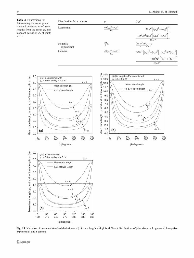
Table 2 Expressions for

determining the mean ll and

standard deviation rl of trace

lengths from the mean la and

standard deviation ra of joints

size a

Distribution form of g(a) ll (rl)2

Lognormal pM lað Þ2þ rað Þ2½ �4la

32M2 lað Þ2þ rað Þ2h i3

�3p2M2 lað Þ2 lað Þ2þ rað Þ2h i2

48 lað Þ4

Negative

exponential

pM2

la 16�p2ð ÞM2

4lað Þ2

Gamma pM lað Þ2þ rað Þ2½ �4la

32M2 lað Þ2þ rað Þ2h i

lað Þ2þ2 rað Þ2h i

�3p2M2 lað Þ2þ rað Þ2h i2

48 lað Þ2

0.0

1.0

2.0

3.0

4.0

5.0

6.0

7.0

8.0

9.0

0 30 60 90 120 150 180

k = 8

k = 2

k = 4

330270240210180 360300

0 30 60 90 120 150 180330270240210180 360300

0 30 60 90 120 150 180330270240210180 360300

β (degrees)

g (a) is Lognormal withµa = 8.0 m and σa = 4.0 m

k = 1

k = 1

Mean trace length

s. d. of trace length

Mea

n tr

ace

leng

th, µ

l, an

d s.

d. o

f tra

ce le

ngth

, σl (

m)

(a)0.0

1.0

2.0

3.0

4.0

5.0

6.0

7.0

8.0

9.0

10.0

11.0

12.0

13.0

14.0

k = 8

k = 2

k = 4

β (degrees)

g (a) is Negative Exponential withµa = σa = 8.0 m k = 1

k = 1

Mean trace length


Mea

n tr

ace

leng

th, µ

l, an

d s.

d. o

f tra

ce le

ngth

, σl (

m)

(b)

0.0

1.0

2.0

3.0

4.0

5.0

6.0

7.0

8.0

9.0

k = 8

k = 2

k = 4

β (degrees)

g (a) is Gamma withµa = 8.0 m and σa = 4.0 m

k = 1

k = 1

Mean trace length


Mea

n tr

ace

leng

th, µ

l, an

d s.

d. o

f tra

ce le

ngth

, σl (

m)

(c)

Fig. 13 Variation of mean and standard deviation (s.d.) of trace length with b for different distributions of joint size a: a Lognormal, b negative

exponential, and c gamma


123

‘‘flat’’ trace length part of Fig. 13), or respectively in some

b ranges approximately symmetrical about b = 90�. It

should be noted that the comments above are simply

assumptions, because no information about the b values

can be found in the original papers or reports.

6 Determination of Joint Shape from Trace Data

The discussion of observed joint shapes has shown that

some joints are elliptical (possibly circular but rarely).

Such joints occur in unbounded or weakly bounded rock.

On the other hand, bounded joints are usually rectangular.

To determine joint shape from joint traces, the following

general two-step process can be followed:

Step 1 Evaluation of geologic information

Based on geologic information mostly from outcrops or

general knowledge of the area, evaluate the possible

shape of fractures. Information from outcrops may be

limited in which case educated assumptions need to be

made if the fracture can be approximated by an ellipse or

a rectangle. Joints not affected by adjacent geological

structures such as bedding boundaries or pre-existing

fractures tend to be elliptical, but joints affected by or

intersecting such geological structures tend to be

rectangles.

Step 2 Characterize joints from joint traces

Based on measured trace lengths on different sampling

planes, joints can be characterized following the proce-

dures in Sects. 6.1 and 6.2, respectively, for elliptical

and rectangular joints.

6.1 Characterization of Elliptical Joints

For elliptical joints, the procedure of Zhang et al. (2002) as

outlined below can be followed to estimate joint shape and

size:

(a) Obtain the trace length data on different sampling

windows (outcrops) and obtain the true trace length

distribution by considering the sampling biases (Priest

and Hudson 1981; Zhang and Einstein 2000).

(b) Assume a major axis orientation and compute the b(the angle between joint major axis and trace line)

value for each sampling window (see Fig. 12).

(c) For the assumed major axis orientation, compute la

and ra of the joint size, using expressions derived

from the general stereological relationship (Eq. 1),

from the trace length data of each sampling window,

by assuming different aspect ratios k and different

distribution forms of g(a). The results are then used to

draw the curves relating la (and ra) to k, respectively,

for the assumed distribution forms of g(a) [see, e.g.,

Fig. 14 for assumed lognormal distribution of g(a)].

(d) Repeat steps (b) and (c) until the curves relating la

(and ra) to k for different sampling windows intersect

in one point (see, e.g., Fig. 14b). The major axis

orientation for this case is the inferred actual major

axis orientation. The k, la and ra values at the

intersection points are the corresponding possible

characteristics of the joints.

6.2 Characterization of Rectangular Joints

For rectangular joints, one of the following three methods

can be used to characterize joint shape and size. It is also

Fig. 14 Variation of la and ra with aspect ratio k for assumed major

axis orientation of a 0�/0�, b 30�/0�, and c 60�/0� (after Zhang et al.

2002)


123

possible to combine two or all of the three methods for the

characterization.

Method 1 Simply measure the joint traces on exposed

bedding surfaces and geometrically infer rectangles

based on simple geometry. The characterization of joints

in isolated sandstone layers by Petit et al. (1994) can be

considered an example of this method.

Method 2 Follow the procedure of Zhang et al. (2002) as

described in Sect. 6.1 to estimate joint shape and size;

but the stereological relationship specifically for rectan-

gular joints will be used. For example, the general

stereological relationship between trace length distribu-

tion and joint size distribution derived by Warburton

(1980b) for parallelograms can be used, a rectangle

being a parallelogram with right angles. Using Warbur-

ton’s stereological relationship, the expressions for

determining the mean and standard deviation of joint

size from the mean and standard deviation of trace

lengths can be derived for different distributions of joint

size. In these expressions, the orientation of a sampling

window is defined by the angle between a side of the

rectangle and the trace line. With these derived expres-

sions, the procedure of Zhang et al. (2002) can then be

used to estimate the joint shape and size.

Method 3 Treat rectangular joints as ellipses at the same

aspect ratio and follow the procedure of Zhang et al.

(2002) as described in Sect. 6.1 to estimate joint shape

and size. The appropriateness of using ellipses to

represent rectangular joints is discussed in Sect. 6.3.

6.3 Using Ellipses to Represent Rectangular Joints

Consider an ellipse and a rectangle which have the same

area and the same aspect ratio (see Fig. 15), i.e.,

pab=4 ¼ LW ð3Þa=b ¼ L=W ¼ k ð4Þ

where a and b are respectively the major and minor axis

length of the ellipse; and L and W are respectively the

length and width of the rectangle. From Eqs. 3 and 4, L and

W can be related respectively to a and b as follows

L ¼ffiffiffipp

2a ¼ 0:87a ð5Þ

W ¼ffiffiffipp

2b ¼ 0:87b ð6Þ

If the centers of the ellipse and rectangle are at the same

location and their major axes are in the same direction, the

area of the rectangle covered by the ellipse (the shaded area

in Fig. 15) can be obtained as

Ac ¼ab

2

ffiffiffipp

ffiffiffiffiffiffiffiffiffiffiffi4� pp

2þ sin�1

ffiffiffipp

2

� �� sin�1


2

� ��

ð7Þ

So the ratio of the covered area to the total area of the

rectangle is

Ac

At¼ 2

p

ffiffiffipp


2þ sin�1

ffiffiffipp

2

� �� sin�1


2

� ��

¼ 0:91

ð8Þ

A ratio greater than 0.91 will result for joints bounded by

straight bedding boundaries but having curved ends such as

those shown in Figs. 5 and 6.

One can thus state that since the ellipse covers over 90%

of the rectangle, it is usually appropriate to use elliptical

joints to represent rectangular joints. Using an elliptical

approximation has the advantage that its size and shape can

be obtained from trace length data (as proposed by Zhang

et al. 2002). This holds even more for polygonal joints with

a larger number of sides, say [5. Clearly, the reverse, i.e.,

multisided polygons can be used to represent ellipses is

also applicable (see Fig. 10). This may be one of the rea-

sons why polygons are used to represent joints in discrete

fracture codes.

7 Summary and Conclusions

A brief literature review about the shape of rock joints has

been conducted. In the literature, some actual observations

of joint shape have been made based on information on

joint surface-morphology, while many researchers have

used trace length observations to approximately infer joint

shapes. Researchers have also conducted experimental

studies on the shape of joints. The literature review is

x

y

0 a/2

b/2C (L/2, W/2)

Ellipse and rectangle have the same area and the same aspect ratio, i.e. πab = LW and a/b = L/W = k,which lead to aL )/( 2π= and bW )/( 2π=

Fig. 15 Representing a rectangle by an ellipse with the same area and

the same aspect ratio


123

followed by the analysis of the available data, the inves-

tigation of the effect of sampling plane orientation on trace

lengths, the discussion of the appropriateness of using

elliptical joints to represent polygonal joints, and the pre-

sentation of methods for characterizing joint shape and size

from trace length data. Based on the analysis and investi-

gation results, the following conclusions can be drawn:

1. Joints not affected by adjacent geological structures

such as bedding boundaries tend to be elliptical (or

approximately circular but rarely), while joints

affected by or intersecting geological structures such

as bed boundaries tend to be most likely rectangles or

similarly shaped polygons.

2. Even for non-equidimensional (elliptical or rectangu-

lar) joints, the average trace lengths on two sampling

planes can be about equal. So the conclusion that rock

joints are equidimensional (circular) drawn from the

fact that the average trace lengths on two sampling

planes are approximately equal can be wrong.

3. To estimate the shape and size of elliptical joints from

trace length data, the procedure of Zhang et al. (2002)

can be followed.

4. Rectangular joints can be characterized by simple

measurements of joint traces on exposed bedding

surfaces and geometrical inferences based on simple

geometry. Alternatively, the general stereological

relationship between trace length distribution and joint

size distribution for rectangular joints can be used to

characterize rectangular joints by following the pro-

cedure of Zhang et al. (2002). Finally, since elliptical

joints can be used to reasonably represent polygonal,

including rectangular joints or vice versa, the shape

and size of rectangular joints can also be estimated

from trace length data by treating them as elliptical

joints and again following the procedure of Zhang

et al. (2002).

Because so many factors affect the shape of joints, it is

possible that the real joint shape is different from what was

described above. Nevertheless, the conclusions presented

above could be used as an initial guideline for joint

characterization.

References

Ameen MS (1995) Fractography: fracture topography as a tool in

fracture mechanics and stress analysis. The Geological Society,

London

Baecher GN, Lanney NA, Einstein HH (1977) Statistical description

of rock properties and sampling. In: 18th US symposium on rock

mechanics, 5C1-8

Bahat D (1988) Fractographics determination of joint length distri-

bution in chalk. Rock Mech Rock Eng 21(1):79–94

Bahat D, Bankwitz P, Bankwitz E (2003) Preuplift joints in granites:

evidence for subcritical and postcritical fracture growth. GSA

Bull 115(2):148–146

Bankwitz P (1965) Ueber Kluefte: I. Beobachtungen im Thuringis-

chen Schiefergebirge. Geologie 14:241–253

Bankwitz P (1966) Ueber Kluefte: II. Die Bildung der Kluftoberfla-

eche und eine Systematik ihrer Strukturen. Geologie 15:896–941

Bankwitz P (1978) Ueber Kluefte: III. Die Entstehung von Saulenk-

luften. Zeitschrift Geol Wissenschaften 6:285–299

Bankwitz P, Bankwitz E (1984) Beitrag zur Interpretation von

Rupturen. Zeitschrift fur Angewandte Geologie 30:265–271

Barton CM (1977) Geotechnical analysis of rock structure and fabric

in CSA Mine NSW. Applied Geomechanics Technical Paper 24,

Commonwealth Scientific and Industrial Research Organization,

Australia

Baudo A (2001) 1-D Fractal, Geostatistical and abusing analyses of

fractures along a 4 km scanline. MS thesis, The State University

of New York at Buffalo

Becker A, Gross MR (1996) Mechanism for joint saturation in

mechanically layered rocks: an example from Southern Israel.

Tectonophysics 257:223–237

Bridges MC (1976) Presentation of fracture data for rock mechanics.

In: 2nd Australia-New Zealand conference on geomechanics,

Brisbane, pp 144–148

Chan LP (1986) Application of Block theory and simulation

techniques to optimum design of rock excavations. PhD thesis,

University of California, Berkeley

Cloos E (1955) Experimental analysis of fracture patterns. Geol Soc

Am Bull 66(3):241–256

Daneshy AA (1973) Three-dimensional propagation of hydraulic

fractures extending from open holes. In: Application of rock

mechanics—15th symposium on rock mechanics, Custer State

Park, SD, pp 157–179

Dershowitz WS (1998) Discrete feature approach for heterogeneous

reservoir production enhancement. Progress Report: October 1,

1998–December 31, 1998, Golder Associates Inc

Dershowitz WS, Einstein HH (1988) Characterizing rock joint

geometry with joint system models. Rock Mech Rock Eng

21:21–51

Dershowitz WS, Lee G, Geier J, Foxford T, LaPointe P, Thomas A

(1993) FracMan, interactive discrete feature data analysis,

geometric modeling, and exploration simulation. User docu-

mentation, Version 2.3, Golder Associates Inc., Seattle

Einstein HH, Bobet A (2004) Crack coalescence in brittle materials:

an overview. In: Schubert (ed) EUROCK 2004 & 53rd

geomechanics colloquium

Einstein HH, Dershowitz WS (1990) Tensile and shear fracturing in

predominantly compressive stress fields—a review. Eng Geol

29:149–172

Einstein HH, Baecher GB, Veneziano D (1979) Risk analysis for rock

slopes in open pit mines—final technical report, Parts I–V,

USBM J 027 5015, Department of Civil Engineering, MIT,

Cambridge, MA

Gross MR, Bahat D, Becker A (1997) Relations between jointing and

faulting based on fracture-spacing ratios and fault-slip profiles: a

new method to estimate strain in layered rocks. Geology

25(10):887–890

Hodgson RA (1961) Classification of structures on joint surfaces. Am

J Sci 259:493–502

Hoek E (1968) Brittle fracture of rock. In: Stagg KG, Zienkiewicz OC

(eds) Rock mechanics in engineering practice. Wiley, pp 99–124

Horii H, Nemat-Nasser S (1986) Brittle failure in compression:

splitting, faulting and brittle ductile transition. Phil Trans R Soc

Lond Math Phys Sci 319(1549)

ISRM (1978) Suggested methods for the quantitative description of

discontinuities in rock masses. International Society for Rock


123

Mechanics, Commission on standardization of laboratory and

field tests. Int J Rock Mech Min Sci Geomech Abstr 15:319–368

Ivanova V (1995) Three-dimensional stochastic modeling of rock

fracture systems. MS thesis, Massachusetts Institute of Technol-

ogy, Cambridge, MA

Ivanova V (1998) Geologic and stochastic modeling of fracture

systems in rocks. PhD thesis, Massachusetts Institute of Tech-

nology, Cambridge, MA

Kulander BR, Barton CC, Dean SL (1979) The application of

fractography to core and outcrop fracture investigations. U.S.

Department of Energy Report METC/SP-79/3, Morgantown

Energy Research Center, p 175

Kulatilake PHSW, Wu TH, Wathugala DN (1990) Probabilistic

modeling of joint orientation. Int J Num Anal Method Geomech

14:325–250

Kulatilake PHSW, Wathugala DN, Stephansson O (1993) Stochastic

three dimensional joint size, intensity and system modeling and a

validation to an area in Stripa Mine, Sweden. Soils Found

33(1):55–70

Lajtai EZ (1969) Strength of discontinuous rocks in direct shear.

Geotechnique 19(2):218–223

Locsin JLZ (2005) Modeling joint patterns using combinations of

mechanical and probabilistic concepts. PhD thesis, Massachu-

setts Institute of Technology, Cambridge, MA

Mandl G (2005) Rock joints—the mechanical genesis. Springer,

Berlin

Meyer T (1999) Geologic stochastic modeling of rock fracture

systems related to crustal faults. MS thesis, Massachusetts

Institute of Technology, Cambridge, MA

Moriya H, Fujita T, Niitsuma H, Eisenblatter J, Manthei G (2006)

Analysis of fracture propagation behavior using hydraulically

induced acoustic emissions in the Bernburg salt mine, Germany.

Int J Rock Mech Min Sci 43(1):49–57

Petit J-P, Massonnat G, Pueo F, Rawnsley K (1994) Rapport de forme

des fractures de mode 1 dans les roches stratifiees: Une etude de

cas dans le Bassin Permian de Lodeve (France). Bulletin du

Centre de Recherches Elf Exploration Production 18(1):211–229

Pollard DD, Aydin AA (1988) Progress in understanding jointing over

the past century. Geol Soc Am Bull 1001:1181–1204

Price NJ (1966) Fault and joint development in brittle and semi brittle

rock. Pergamon Press, London, 176 p

Priest SD, Hudson J (1981) Estimation of discontinuity spacing and

trace length using scanline surveys. Int J Rock Mech Min Sci

Geomech Abstr 18:13–197

Riedel W (1929) Zur Mechanik Geologischer Brucherscheinungen.

Zentrabl Mineral Abt B 354–68

Robertson A (1970) The interpretation of geologic factors for use in

slope theory. In: Proceedings of symposium on the theoretical

background to the planning of open pit mines, Johannesburg,

South Africa, pp 55–71

Saltzman B (2001) Possible correlation between mechanical layer’s

joint spacing and its rock mechanical properties. MS thesis, Ben

Gurion University of the Negev

Savalli L, Engelder T (2005) Mechanisms controlling rupture shape

during subcritical growth of joints in layered rocks. GSA Bull

117(3/4):436–449

Sheldon P (1912) Some observations and experiments on joint planes.

J Geol 20:164–183

Song J-J (2006) Estimation of areal frequency and mean trace length

of discontinuities observed in non-planar surfaces. Rock Mech

Rock Eng 39(2):131–146

Song J-J, Lee C-I (2001) Estimation of joint length distribution using

window sampling. Int J Rock Mech Min Sci 38(4):519–528

Villaescusa E, Brown ET (1990) Maximum likelihood estimation of

joint size from trace length measurements. Rock Mech Rock Eng

25:67–87

Warburton PM (1980a) A stereological interpretation of joint trace

data. Int J Rock Mech Min Sci Geomech Abstr 17:181–190

Warburton PM (1980b) Stereological interpretation of joint trace

data: influence of joint shape and implications for geological

surveys. Int J Rock Mech Min Sci Geomech Abstr 17:305–316

Wathugala DN (1991) Stochastic three dimensional joint geometry

modeling and verification. PhD dissertation, University of

Arizona, Tucson

Weinberger R (2001) Joint nucleation in layered rocks with non-

uniform distribution of cavities. J Struct Geol 23:1241–1254

Woodworth JB (1896) On the fracture system of joints, with remarks

on certain great fractures. Boston Soc Nat Hist Proc 27:163–184

Zhang L (2005) Engineering properties of rocks. Elsevier, p 304

Zhang L, Einstein HH (2000) Estimating the intensity of rock

discontinuities. Int J Rock Mech Min Sci 37:819–837

Zhang L, Einstein HH, Dershowitz WS (2002) Stereological

relationship between trace length distribution and size distribu-

tion of elliptical discontinuities. Geotechnique 52(6):419–433


123

art-3a10.1007-2fs00603-009-0054-0

Documents

conclusionthat rock

planar shape ofdiscontinuities

realdiscontinuity shape

real discontinuity shape

tension joints

similar polygonal joints

common discontinuities

connectivityof discontinuities