arimax arima
DESCRIPTION
difference between arima and arimaxTRANSCRIPT
Building ARIMA and ARIMAX Models for
Predicting Long-Term Disability Benefit Application
Rates in the Public/Private Sectors
Sponsored by
Society of Actuaries
Health Section
Prepared by
Bruce H. Andrews
Matthew D. Dean
Robert Swain
Caroline Cole
University of Southern Maine August 2013
© 2013 Society of Actuaries, All Rights Reserved
The opinions expressed and conclusions reached by the authors are their own and do not represent any official position or opinion
of the Society of Actuaries or its members. The Society of Actuaries makes no representation or warranty to the accuracy of the
information.
© 2013 Society of Actuaries, All Rights Reserved University of Southern Maine
EXECUTIVE SUMMARY
Using the Social Security Disability Insurance benefit claim rate as a proxy, this study
investigates two statistical approaches to forecasting long-term disability benefit claims. The
results are extendable and should prove useful for insurance carriers who wish to predict short-
term future levels of long-term disability benefit claims. The study demonstrates that both the
autoregressive integrated moving average (ARIMA) and autoregressive integrated moving
average with exogenous variables (ARIMAX) methodologies have the ability to produce
accurate four-quarter forecasts.
First built was an ARIMA model, which produces forecasts based upon prior values in the time
series (AR terms) and the errors made by previous predictions (MA terms). This typically allows
the model to rapidly adjust for sudden changes in trend, resulting in more accurate forecasts.
Next built was an ARIMAX model, which is very similar to an ARIMA model, except that it
also includes relevant independent variables. While the inclusion of exogenous variables adds
complexity to the model-building process, the model can capture the influence of external factors
(e.g., the state of the economy) as well as management controllables (e.g., elimination period
duration).
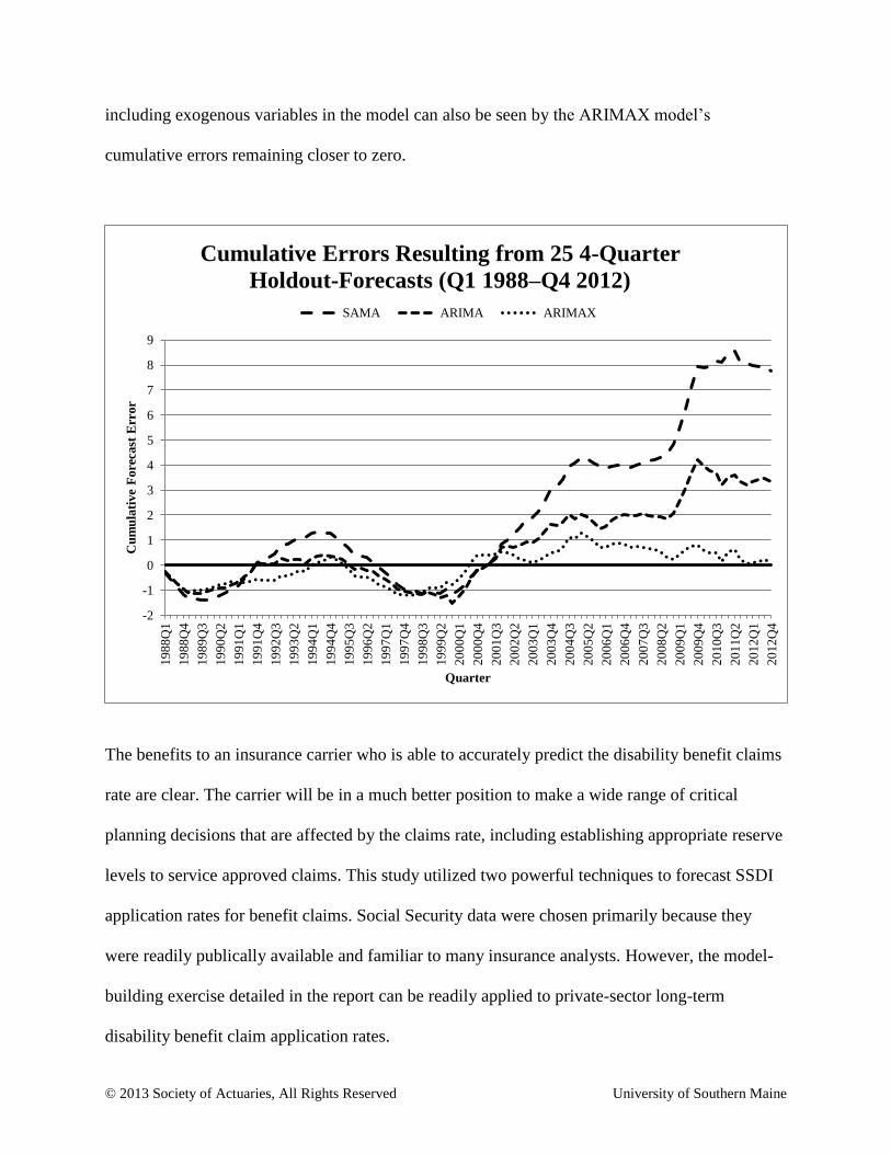
The superior performance of both the ARIMA and ARIMAX models against the commonly used
seasonally adjusted four-quarter moving average (SAMA) model can be seen in the following
graph. Both models’ cumulative errors tend to remain close to zero, while the SAMA model’s
cumulative errors deviate from zero more dramatically. The additional beneficial impact of
© 2013 Society of Actuaries, All Rights Reserved University of Southern Maine
including exogenous variables in the model can also be seen by the ARIMAX model’s
cumulative errors remaining closer to zero.
The benefits to an insurance carrier who is able to accurately predict the disability benefit claims
rate are clear. The carrier will be in a much better position to make a wide range of critical
planning decisions that are affected by the claims rate, including establishing appropriate reserve
levels to service approved claims. This study utilized two powerful techniques to forecast SSDI
application rates for benefit claims. Social Security data were chosen primarily because they
were readily publically available and familiar to many insurance analysts. However, the model-
building exercise detailed in the report can be readily applied to private-sector long-term
disability benefit claim application rates.
-2
-1
0
1
2
3
4
5
6
7
8
9
19
88
Q1
19
88
Q4
19
89
Q3
19
90
Q2
19
91
Q1
19
91
Q4
19
92
Q3
19
93
Q2
19
94
Q1
19
94
Q4
19
95
Q3
19
96
Q2
19
97
Q1
19
97
Q4
19
98
Q3
19
99
Q2
20
00
Q1
20
00
Q4
20
01
Q3
20
02
Q2
20
03
Q1
20
03
Q4
20
04
Q3
20
05
Q2
20
06
Q1
20
06
Q4
20
07
Q3
20
08
Q2
20
09
Q1
20
09
Q4
20
10
Q3
20
11
Q2
20
12
Q1
20
12
Q4
Cu
mu
lati
ve
Fore
cast
Err
or
Quarter
Cumulative Errors Resulting from 25 4-Quarter
Holdout-Forecasts (Q1 1988–Q4 2012)
SAMA ARIMA ARIMAX

© 2013 Society of Actuaries, All Rights Reserved University of Southern Maine
Page 1
BUILDING ARIMA and ARIMAX MODELS
for
PREDICTING LONG-TERM DISABILITY BENEFIT APPLICATION RATES
in the
PUBLIC/PRIVATE SECTORS

© 2013 Society of Actuaries, All Rights Reserved University of Southern Maine
Page 2
ACKNOWLEDGEMENTS
The authors are extremely grateful for the financial support provided by the Society of
Actuaries and for their compassion in granting “no cost” extensions. In addition, the authors also
wish to thank the Maine Center for Business and Economic Research for its generous financial
support.
© 2013 Society of Actuaries, All Rights Reserved University of Southern Maine
Page 3
1. INTRODUCTION
1.1 Purpose of the Study
The Maine Center for Business and Economic Research (MCBER) at the University of Southern
Maine, in partnership with the Society of Actuaries (SOA), conducted a predictive model-
building exercise to statistically examine and incorporate factors that influence long-term
disability (LTD) application rates. This report documents that study. Social Security
Administration (SSA) claims-experience data were selected for the model building because they
are publicly available and representative (in varying degrees) of the private-sector LTD claims
experience. Private LTD carrier data were deemed inappropriate for use in this study because
they vary in form, level of detail and their period of collection. Further, it was thought that LTD
carriers would find it awkward to share or pool their data with other carriers because they
frequently compete in the same markets.
Many of the phenomena that drive Social Security disability application rates are likely to
influence LTD application rates for private carriers, which means that exogenous variables that
are significant predictors of Social Security Disability Insurance (SSDI) application rates are
likely to be strong predictors for private carriers as well. Also, the future experience of at least
some private-sector carriers was expected to display a statistical relationship with the application
rates projected for Social Security disability.
This study focuses most heavily on the autoregressive integrated moving average with
exogenous variables (ARIMAX) methodology, which has the capacity to identify the underlying
patterns in time-series data and to quantify the impact of environmental influences. This provides
© 2013 Society of Actuaries, All Rights Reserved University of Southern Maine
Page 4
the ARIMAX modeler with the capacity to isolate the influences of high-impact changes of both
an external nature (e.g., competitors’ activities, the economy and governmental regulations) and
an internal nature (e.g., policy coverage, product pricing and target markets). It is also important
to note that ARIMAX model building can be reduced/simplified to pure autoregressive
integrated moving average (ARIMA) model building if the forecaster/modeler wishes to examine
historical behavior and make projections employing only statistically identified historical
patterns/relationships.
The target audience for this report is the actuary who either has a basic working knowledge of
applied multiple-linear-regression model building or is willing to invest the energy to
acquire/recover it. This prerequisite level of understanding of multiple-regression analysis is that
which is typically derived from the one or two 3-credit (noncalculus-based) undergraduate
courses in applied business statistics required at nationally accredited business schools. As
further encouragement for the tentative reader to press forward, the two student co-authors of
this report, Bob Swain and Caroline Cole, have completed only the six credits of undergraduate-
level statistics required by the business school at the University of Southern Maine.
1.2 Background
To coarsely evaluate the strength of the potential relationship between the application rates for
SSDI and those of group LTD carriers, annual data from 2004–10 from 12 of the largest private-
sector carriers were examined. Six of the 12 carriers had annual application rates that were
significantly correlated ( ≤ 0.10) with SSDI’s annual application rates at lags of 0, 1 and/or 2.
Four of these six exhibited one or more significant positive correlations; the other two displayed

© 2013 Society of Actuaries, All Rights Reserved University of Southern Maine
Page 5
significant negative correlations, one at lag 1 and the other at lags 1 and 2. (It is important to note
that the coarseness of the data and the small sample [n=7] placed serious constraints on this
statistical analysis.)
Accurate prediction of future application rates for long-term disability benefits is a major
concern for private insurance carriers as well as the Social Security Administration. In both the
private and public sectors, the number of claims filed is a key input to many planning decisions.
For example, in both sectors, the proper level of reserves required to service approved claims
needs to be established, mechanisms to generate revenue streams must be created to maintain
appropriate reserve levels, and claims processing and management capacity requirements must
be estimated. Unfortunately, application rates are extremely volatile because they are largely
driven by forces external to the insurer, be it the SSA in the public sector or an LTD provider in
the private sector. For example, at the national level, SSDI applications increased substantially1
during six of the seven U.S. recessions between 1965 and 2012.2 Further, a December 2011
article in the Wall Street Journal,3 titled “Jobless Tap Disability Fund,” reported on the findings
of researchers who have studied the interaction between the condition of the U.S. economy and
the SSDI application rate. Some of their findings are summarized below.
Professor Mark Duggan at the University of Pennsylvania studied the relationship
between the U.S. unemployment rate and the application rate for SSDI benefits, and
“estimates that the higher unemployment rate [in 2011 compared to 2007] accounts
for 3,000 additional people applying for benefits each week.”
1 Social Security Administration, “Disabled Workers.”
2 Wikipedia contributors, “List of recessions in the United States.”
3 Paletta and Searcey, “Jobless Tap Disability Fund.”

© 2013 Society of Actuaries, All Rights Reserved University of Southern Maine
Page 6
Steven Goss, chief actuary of the Social Security Administration, “told Congress …
that the 2008–09 recession led to a higher rate of ‘disability incidence’ than any other
period except for the economic downturn in 1975.”
Professor Matthew Rutledge at Boston College studied the relationship between time
left until unemployment benefits expire and the likelihood an individual would apply
for SSDI benefits, and found that the unemployed are “significantly more likely to
apply when [unemployment payments are] ultimately exhausted,” indicating that
long-term unemployment is positively linked to the SSDI application rate.
Massachusetts Institute of Technology professor of economics David Autor summed
up his sentiments this way: “To a very large extent, [SSDI] is our big welfare
program.”
Some of the other 16 major determinants of the disability application rate listed in Actuarial
Study No. 118 produced by the SSA’s Office of the Actuary4 include the strength of regional
economies, demographic shifts, levels of employment/unemployment and levels of inflation.
1.3 The ARIMAX Methodology
Proper ARIMAX model building has six statistical assumptions that must be addressed and re-
addressed as iterative model building progresses. These six assumptions also provide the
underpinnings for rigorously performed multiple-regression analysis. While the rules of properly
performed regression analysis are rarely fully honored by nonacademic practitioners, when
satisfied, they normally lead to much-improved model-building results.
4 Zayatz, “Social Security Disability.”

© 2013 Society of Actuaries, All Rights Reserved University of Southern Maine
Page 7
Simply put, an ARIMAX model can be viewed as a multiple regression model with one or more
autoregressive (AR) terms and/or one or more moving average (MA) terms. Autoregressive
terms for a dependent variable are merely lagged values of that dependent variable that have a
statistically significant relationship with its most recent value. Moving average terms are nothing
more than residuals (i.e., lagged errors) resulting from previously made estimates.
So, for example, a nameless time-series dependent variable might be well estimated by a
properly weighted combination of the following four right-hand-side (RHS) variables.
1. = the value of the independent variable at time
2. = the immediately preceding value of the dependent variable at time
3. = the immediately preceding value of the dependent variable at time
4. = the estimation error produced by the model at time
This single-independent-variable, multiple-regression-like model for estimating the dependent
variable relies on the predictive value of the independent variable (unlagged), the dependent
variable itself (lagged by 1), the dependent variable again (lagged by 2) and a previously
produced error term (lagged by 4). That is,
,
where , , and are estimated coefficients.
As implied by its shortened acronym, the pure ARIMA model-building methodology employs
only lagged values of the dependent variable (i.e., AR terms) and lagged values of errors
previously produced by the model (i.e., MA terms). The I in ARIMA refers to integrated and
indicates that the dependent variable time series has been differenced one or more times to make

© 2013 Society of Actuaries, All Rights Reserved University of Southern Maine
Page 8
the time series stationary before model building begins. (Note: Practically speaking, stationarity
implies that the mean and the variance of the time series are not changing over time.) So, for
example, the quarterly application rate for SSDI benefits time series used illustratively in this
report has displayed a strong overall pattern characterized by both an upward trend and quite-
regular quarterly seasonality. As discussed in Section 2.1, to remove the quarterly seasonality,
the raw data were differenced by four and then differenced by one to remove the upward trend.
The core difference between formal ARIMAX modeling and the more commonly used multiple
regression modeling is that the ARIMAX modeling rigorously adheres to all six of the statistical
assumptions underlying regression modeling. Section 2.2 explains these six assumptions. The
ARIMAX model-building algorithm flowchart (Figure 8) makes clear the complexity of the
iterative process. This level of complexity sometimes discourages model builders from fully
adhering to the full set of six key assumptions required for proper regression modeling.
Assumption 3 provides one example of the complexities of meticulously executed regressive
modeling in that proper interpretation of the significance levels ( -values) of regression-model
coefficients requires that the residuals produced by the model under scrutiny are normally
distributed with a mean of zero, a constant variance and (most importantly) with no serial
correlation. To satisfy these formal assumptions, it is frequently necessary to model the residuals
with ARIMA tools, which often forces originally identified, logically attractive independent
variables to lose their significance and to leave the model. This removal of independent variables
that appeared to be strong candidates changes the form and character of the residuals and may
result in a complete restart of the model-building process.
© 2013 Society of Actuaries, All Rights Reserved University of Southern Maine
Page 9
To address the complex, iterative nature of the ARIMAX model-building process when the pool
of explanatory-variable candidates is large, MCBER built a system of integrated SAS5 software
routines to automate the search for the optimal or near-optimal combination of exogenous
variables, and AR and MA terms. The resulting ARIMAX models are statistically correct in all
regards. Additionally, the composition of both models built using the SAS routines on the
illustrative quarterly SSDI-application-rate data set (Q1 1982–Q4 2012) are very intuitively
appealing. After differencing by four (to remove seasonality) and then one (to remove trend), the
(AR1, AR3, AR10, MA4) ARIMA model produced the best fit with a mean error of 0.005901
and a standard error of 0.0138 for the residuals. The -values for the coefficients for the AR1,
AR3, AR10 and MA4 terms were 0.0002, 0.0035, 0.0045 and < 0.0001, respectively. For the
doubly differenced time series, this means that the ARIMA model was built by weighting the
most recent actual, the actual three quarters earlier, the actual 10 quarters earlier and the
estimation error made four quarters earlier. That is,
.
The best-fitting ARIMAX model (not coincidentally) has a structure similar to the previous
ARIMAX model for the “nameless” dependent variable introduced on Page 7. The AR1 and MA4
terms from the ARIMA model were accompanied by wage-and-salary employment (wse) (lag 0) and
an AR2 term. That is,
.
5 http://www.sas.com
© 2013 Society of Actuaries, All Rights Reserved University of Southern Maine
Page 10
This model produced a mean error of 0.004823 and a standard error of 0.0130. The -value for
the coefficients of the AR1, MA4 and the independent variable were all ≤ 0.0001, and the -
values for the AR2 term was 0.0058. The fitting and forecasting capacities of the ARIMA and
ARIMAX models are discussed in further detail on pages 50-52.
1.4 Comparison of ARIMAX and SAMA Models
To examine the relative precision of the best-fitting ARIMAX model, its fit performance was
compared against that of the commonly used seasonally adjusted four-quarter moving average
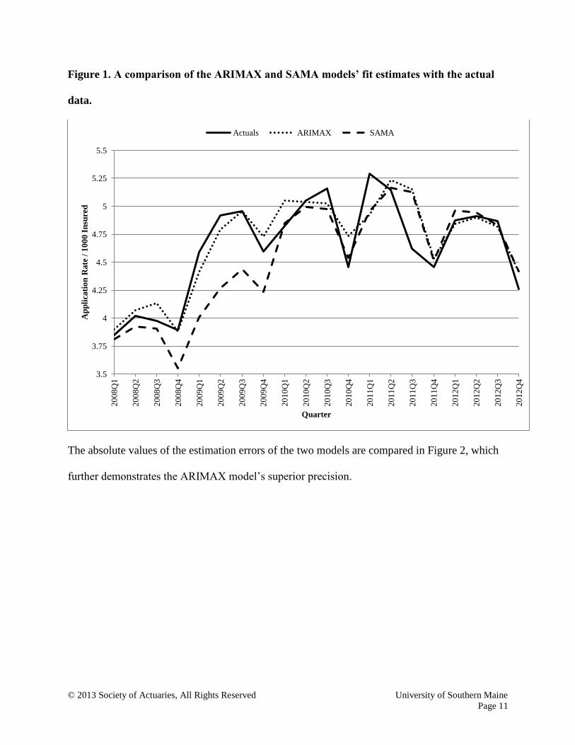
(SAMA) model. Figure 1 shows the 20 most recent actual quarterly SSDI application rates and
the fit estimates produced by each model. The ARIMAX model clearly does a better job of
estimating the actual application rates, particularly during periods of steady rising or declining.
© 2013 Society of Actuaries, All Rights Reserved University of Southern Maine
Page 11
Figure 1. A comparison of the ARIMAX and SAMA models’ fit estimates with the actual
data.
The absolute values of the estimation errors of the two models are compared in Figure 2, which
further demonstrates the ARIMAX model’s superior precision.
3.5
3.75
4
4.25
4.5
4.75
5
5.25
5.5
20
08
Q1
20
08
Q2
20
08
Q3
20
08
Q4
20
09
Q1
20
09
Q2
20
09
Q3
20
09
Q4
20
10
Q1
20
10
Q2
20
10
Q3
20
10
Q4
20
11
Q1
20
11
Q2
20
11
Q3
20
11
Q4
20
12
Q1
20
12
Q2
20
12
Q3
20
12
Q4
Ap
pli
cati
on
Rate
/ 1
00
0 I
nsu
red
Quarter
Actuals ARIMAX SAMA

© 2013 Society of Actuaries, All Rights Reserved University of Southern Maine
Page 12
Figure 2. A comparison of the ARIMAX and SAMA models’ absolute errors.
The mean absolute percent errors (MAPEs) and mean absolute deviations (MADs) for both
models over all 116 quarters for which both models produce estimates (Q1 1984–Q4 2012) and
for the most recent 20 quarters (Q1 2008–Q4 2012) are shown in Chart 1.
Chart 1. A comparison of the ARIMAX and SAMA models’ goodness-of-fit over two
different time horizons.
Q1 1984–Q4 2012 Q1 2008–Q4 2012
MAPE MAD MAPE MAD
ARIMAX
3.42%
0.10
2.85%
0.13
SAMA
4.50%
0.14
4.54%
0.21
0.00000
0.10000
0.20000
0.30000
0.40000
0.50000
0.60000
0.70000
0.80000 2
00
8Q
1
20
08
Q2
20
08
Q3
20
08
Q4
20
09
Q1
20
09
Q2
20
09
Q3
20
09
Q4
20
10
Q1
20
10
Q2
20
10
Q3
20
10
Q4
20
11
Q1
20
11
Q2
20
11
Q3
20
11
Q4
20
12
Q1
20
12
Q2
20
12
Q3
20
12
Q4
Ab
solu
te E
rrors
Quarter
ARIMAX SAMA

© 2013 Society of Actuaries, All Rights Reserved University of Southern Maine
Page 13
Once again, the ARIMAX model clearly outperforms the SAMA model based on its lower
MAPEs and MADs for both time periods. In comparison with the SAMA model, the ARIMAX
model’s MAPEs improve by 24 percent and 37 percent, and its MADs improve by 29 percent
and 38 percent.
1.5 The Dependent Variable
While disability insurance award rates (i.e., approval rates) are somewhat influenced by the
previously mentioned 16 factors, they are also determined by forces internal to the insurance
provider such as organizational goals, strategies, policies and practices created and administered
from within. This tends to reduce the volatility in approval rates and makes them more
predictable than application rates. Not surprisingly, as seen in Figure 3, the application rates for
SSDI among insured workers have exhibited much more variability than the acceptance rates
among SSDI applicants. During the 31-year period of this study (1982–2012), the quarterly
application rate per 1,000 insured workers ranged from a low of 1.929 in Q4 1999 to a high of
5.292 in Q1 2011, a rise of almost 274 percent. Over the 124 quarters in the data set, the
application rate mean was 3.046 and the standard deviation was 0.869, yielding a coefficient of
variation ( ) of 0.285. During the same period, the quarterly award rate, which is the
proportion of applications approved, was relatively flat, ranging from 0.255 to 0.558, with a
mean of 0.411 and a standard deviation of 0.063, yielding a considerably smaller coefficient of
variation of 0.153. (Note that the coefficient of variation for application rates is 86.3 percent
larger than that for award rates.) Figure 3 makes clear the contrast in the long-term slope and the
volatility of the two time series.

© 2013 Society of Actuaries, All Rights Reserved University of Southern Maine
Page 14
Figure 3. Application and award rates for social security disability benefits.
This study focuses on modeling the more highly volatile, publicly available quarterly SSDI-
application-rate/1000 insured time series presented in Figure 3. It serves well as a surrogate for
private-sector submitted LTD claims experience in building time-series forecasting models.
While the application-rate time-series patterns in the private sector are not created by all of the
same forces that drive public-sector demand for disability payments, there are certainly many
overlaps. In both settings, regional and national economic conditions heavily influence the rate
of applications as do medical advancements and breakthroughs in the treatment of specific
disorders. Other common influences include demographic shifts (e.g., aging baby boomers),
technological improvements that can enhance one’s ability to work and level of participation of
females in the workforce.
0
1
2
3
4
5
6
19
82
Q1
19
82
Q4
19
83
Q3
19
84
Q2
19
85
Q1
19
85
Q4
19
86
Q3
19
87
Q2
19
88
Q1
19
88
Q4
19
89
Q3
19
90
Q2
19
91
Q1
19
91
Q4
19
92
Q3
19
93
Q2
19
94
Q1
19
94
Q4
19
95
Q3
19
96
Q2
19
97
Q1
19
97
Q4
19
98
Q3
19
99
Q2
20
00
Q1
20
00
Q4
20
01
Q3
20
02
Q2
20
03
Q1
20
03
Q4
20
04
Q3
20
05
Q2
20
06
Q1
20
06
Q4
20
07
Q3
20
08
Q2
20
09
Q1
20
09
Q4
20
10
Q3
20
11
Q2
20
12
Q1
20
12
Q4
Quarter
Award Rate / Application Application Rate / 1000 Insured
© 2013 Society of Actuaries, All Rights Reserved University of Southern Maine
Page 15
2. CONSTRUCTION AND VALIDATION OF ARIMA AND ARIMAX MODELS
Section 2.1, Construction and Validation of an ARIMA Model, focuses on explaining and
illustrating the steps in the methodology for constructing a pure ARIMA model. This illustration
employs the previously introduced 124-point quarterly SSDI-application-rate time series (Q1
1982–Q4 2012). This discussion also includes all of the statistical assumptions that must be
satisfied for an ARIMA model to be valid. Results from the analysis of residuals from final
ARIMA and ARIMAX models are examined to ensure they meet the necessary conditions.
Model-fitting results are then presented and evaluated using standard goodness-of-fit measures
produced by the fitting process. In addition, the accuracy/precision of the holdout forecasts
produced by the final pure ARIMA model are examined.
Section 2.2, Construction and Validation of an ARIMAX Model, is heavily patterned after
Section 2.1, but focuses on explaining and illustrating the step-by-step methodology for building
and validating an ARIMAX model. This discussion also includes an explanation of the much-
expanded series of statistical assumptions that must be satisfied for an ARIMAX model to be
valid. In keeping with the ARIMA discussion in Section 2.1, results from the analysis of
residuals are reviewed and the quality of the ARIMAX model is evaluated in the context of both
in-sample fitting and holdout-sample forecasting. Lastly, both sets of goodness-of-fit statistics
are compared with their counterparts produced by the pure ARIMA model to assess the
incremental explanatory value contributed by the exogenous variables.

© 2013 Society of Actuaries, All Rights Reserved University of Southern Maine
Page 16
2.1 Construction and Validation of an ARIMA Model
The AR (autoregressive) in ARIMA refers to previous (i.e., lagged) values of the dependent-
variable time series. MA (moving average) refers to lagged error terms (i.e., residuals) created by
the ARIMA model’s inability to produce perfectly accurate estimates. So, ARMA (ARIMA
without I) models are similar in appearance to a regression model with all of the right-hand-side
(RHS) variables being lagged versions of the dependent variable and lagged versions of the
error term .
A general order ARMA ( ) model with autogressive terms ( and moving average
terms ( would be represented as
– 6
In terms of structure, ARIMA ( ) models are the same as ARMA ( ) models where the
time series has first been transformed by differencing. The specifies the order of the
differencing. For example, in Figure 5, the original undifferenced ( ) quarterly time series and
the differenced once ( ) time series are graphed. In Figure 6, the original, undifferenced time
series is differenced once ( ) by four, and then these differences are differenced again by one
( ). Since the time series must be stationary before it can be modeled with AR and MA
terms,7 differencing is commonly used to transform a nonstationary time series into a stationary
time series where the mean and variance are statistically judged to be constant.
For example, a repeating daily time series that was strongly influenced by the day of the week
(Sunday–Saturday) might likely be differenced by seven to remove the day-of-week effect. The
6 Montgomery, Jennings, and Kulahci, Introduction to Time Series, 253.
7 SAS Institute Inc. SAS/ETS 9.2, 210.

© 2013 Society of Actuaries, All Rights Reserved University of Southern Maine
Page 17
resulting differenced time series would then represent the week-to-week change in the daily data
and the variance created by the day-of-week effect would be largely removed. At the same time, if
there were no underlying weekly trend in the original time series, then these transformed data
would likely appear to be stationary with a mean close to zero. However, if this same original
(untransformed) time series were increasingly trending up in a quadratic fashion, then the
differenced-by-seven time series would exhibit a positive linear trend (without the day-of-week
influence), and the mean would not be constant over time. To address this lack of stationarity,
differencing the resulting time series by one would remove the upward trend and cause the mean
of the twice-transformed time series to be relatively constant. If both the mean and variance were
indeed constant, the doubly differenced series would be stationary. Conveniently, the degree of
stationarity of the transformed time series may be statistically evaluated using the augmented
Dickey-Fuller test.8
Once a time series is statistically judged to be stationary, ARMA/ARIMA model building may
begin. Identification of AR and MA terms requires the model builder to examine the
autocorrelation coefficient function (ACF) and the partial autocorrelation coefficient function
(PACF), to gain insights into the nature of the serial correlation.9
At the most basic level, there are two types of ARMA/ARIMA models, subset (i.e., additive)10
and order. An order ARMA ( ) model to estimate is comprised of terms involving
and terms involving . In other words, the
autoregressive terms would include lags of 1 through and the moving-average terms would
8 Ibid., 246.
9 Nau, “Identifying the Numbers.”
10 SAS Institute Inc. SAS/ETS 9.2, 212.
© 2013 Society of Actuaries, All Rights Reserved University of Southern Maine
Page 18
include lags 1 through . In contrast, a subset or additive model includes only specified lags for
the autoregressive terms and specified lags for the moving-average terms. Stige et al. states that,
“Subset ARIMA models are often used to obtain parsimonious models that may be more
interpretable than nonsubset ARIMA models,” and cites three other references that discuss their
success in applying subset models.11
The subset model-building approach was chosen for this
effort for these reasons and because it facilitated the identification of models with much more
finely tuned specifications, thus providing more attractive models from which to choose.
Identifying the form of an ARMA or ARIMA model is an iterative process that requires selecting
appropriate differencing schemes to achieve stationarity as signaled by the augmented Dickey-
Fuller test. Then, appropriately lagged AR and MA terms are introduced based on the significant
patterns exhibited by their correlation functions. After the introduction of each AR or MA term,
the residuals are re-examined for significance using the ACF and PACF. The process continues
until these two correlation functions provide no further statistical clues to indicate that any AR or
MA terms are missing. At this point, the Ljung-Box test for white noise12
may be used to
statistically evaluate the degree to which the residuals are free of serial correlation. The statistical
details of this are discussed in Montgomery, Jennings and Kulahci.13
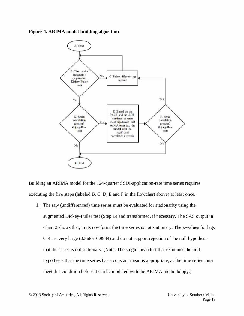
The flowchart in Figure 4 captures the sequence of steps that must be followed to construct a valid
pure ARIMA model. As indicated by the two nested looping structures (BCB and
BDEFCB), this process may take many iterations to complete.
11
Stige, et al., “Thousand-Year-Long Chinese Time Series.” 12
SAS Institute Inc. SAS/ETS 9.2, 194. 13
Montgomery, Jennings, and Kulahci, Introduction to Time Series, 57.
© 2013 Society of Actuaries, All Rights Reserved University of Southern Maine
Page 19
Figure 4. ARIMA model-building algorithm
Building an ARIMA model for the 124-quarter SSDI-application-rate time series requires
executing the five steps (labeled B, C, D, E and F in the flowchart above) at least once.
1. The raw (undifferenced) time series must be evaluated for stationarity using the
augmented Dickey-Fuller test (Step B) and transformed, if necessary. The SAS output in
Chart 2 shows that, in its raw form, the time series is not stationary. The -values for lags
0–4 are very large (0.5685–0.9944) and do not support rejection of the null hypothesis
that the series is not stationary. (Note: The single mean test that examines the null
hypothesis that the time series has a constant mean is appropriate, as the time series must
meet this condition before it can be modeled with the ARIMA methodology.)

© 2013 Society of Actuaries, All Rights Reserved University of Southern Maine
Page 20
Chart 2. SAS output: Augmented Dickey-Fuller test.
Type Lags Pr < Tau
Single Mean 0 0.5685
1 0.8170
2 0.9469
3 0.9944
4 0.9257
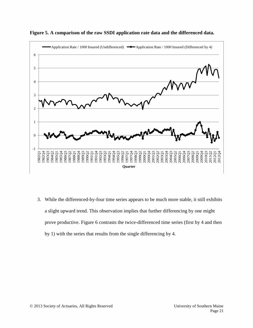
2. In Figure 5, an upward trend in the undifferenced SSDI data is very apparent, as is the
four-period seasonality made evident by the behavior of Q4, which is the smallest quarter
for each of the 31 years. To remove the seasonality, differencing this quarterly time series
by 4 produces a much more stable pattern (Step C). Figure 5 shows that the variance in
the time series is significantly reduced by this transformation. Centered around 0, the
differenced time series ranges from −0.5 to 1.0, in contrast with the original series that
ranges from under 1.9 to over 5.2. Thus, differencing has reduced the sample range from
3.3 to 1.5 (in approximate terms).
© 2013 Society of Actuaries, All Rights Reserved University of Southern Maine
Page 21
Figure 5. A comparison of the raw SSDI application rate data and the differenced data.
3. While the differenced-by-four time series appears to be much more stable, it still exhibits
a slight upward trend. This observation implies that further differencing by one might
prove productive. Figure 6 contrasts the twice-differenced time series (first by 4 and then
by 1) with the series that results from the single differencing by 4.
-1
0
1
2
3
4
5
6
19
82
Q1
19
82
Q4
19
83
Q3
19
84
Q2
19
85
Q1
19
85
Q4
19
86
Q3
19
87
Q2
19
88
Q1
19
88
Q4
19
89
Q3
19
90
Q2
19
91
Q1
19
91
Q4
19
92
Q3
19
93
Q2
19
94
Q1
19
94
Q4
19
95
Q3
19
96
Q2
19
97
Q1
19
97
Q4
19
98
Q3
19
99
Q2
20
00
Q1
20
00
Q4
20
01
Q3
20
02
Q2
20
03
Q1
20
03
Q4
20
04
Q3
20
05
Q2
20
06
Q1
20
06
Q4
20
07
Q3
20
08
Q2
20
09
Q1
20
09
Q4
20
10
Q3
20
11
Q2
20
12
Q1
20
12
Q4
Quarter
Application Rate / 1000 Insured (Undifferenced) Application Rate / 1000 Insured (Differenced by 4)

© 2013 Society of Actuaries, All Rights Reserved University of Southern Maine
Page 22
Figure 6. A comparison of the SSDI application rate data using two different differencing
schemes.
From purely a visual assessment, it appears that the best differencing transformation for
providing a constant mean and minimum variance has been found. (Note: A commonly
used rule of thumb14
is that the optimal order of differencing produces the lowest
standard deviation.) This is further substantiated by examining the five highly significant
(<0.0001) -values for lags 0–4 in the augmented Dickey-Fuller test (Step B) presented
in the single-mean portion of the SAS output shown in Chart 4. The five 0+ -values for
the single-mean model with lags 0–4 support rejection of the five null hypotheses
asserting a unique mean at each lag value (0–4). This implies that the differenced data are
14
Nau, “Identifying the Order.”
-1.5
-1
-0.5
0
0.5
1
1.5
19
82
Q1
19
82
Q4
19
83
Q3
19
84
Q2
19
85
Q1
19
85
Q4
19
86
Q3
19
87
Q2
19
88
Q1
19
88
Q4
19
89
Q3
19
90
Q2
19
91
Q1
19
91
Q4
19
92
Q3
19
93
Q2
19
94
Q1
19
94
Q4
19
95
Q3
19
96
Q2
19
97
Q1
19
97
Q4
19
98
Q3
19
99
Q2
20
00
Q1
20
00
Q4
20
01
Q3
20
02
Q2
20
03
Q1
20
03
Q4
20
04
Q3
20
05
Q2
20
06
Q1
20
06
Q4
20
07
Q3
20
08
Q2
20
09
Q1
20
09
Q4
20
10
Q3
20
11
Q2
20
12
Q1
20
12
Q4
Quarter
Application Rate / 1000 Insured (Differenced by 4) Application Rate / 1000 Insured (Differenced by 1 and 4)

© 2013 Society of Actuaries, All Rights Reserved University of Southern Maine
Page 23
stationary and that there is a single mean. Lastly, while the (1,4) differencing scheme
made the transformed series stationary, the -values from the autocorrelation check for
white noise remained very small and suggested that significant AR and/or MA terms
were needed (Step D) to remove the highly significant autocorrelation still present in the
twice-differenced ( ) series.
Chart 3. SAS output: Autocorrelation check for white noise.
To Chi- Pr >
Lag Square DF ChiSq -------------------Autocorrelations-------------------
6 68.39 6 <.0001 −0.382 −0.019 0.298 −0.514 0.173 0.144
12 72.19 12 <.0001 −0.084 0.043 −0.034 −0.126 0.052 0.013
18 73.53 18 <.0001 0.038 −0.037 −0.073 −0.035 −0.018 −0.009
24 94.93 24 <.0001 0.085 −0.043 −0.072 0.191 −0.213 0.217
Chart 4. SAS output: Augmented Dickey-Fuller test.
Type Lags Pr < Tau
Single Mean 0 <.0001
1 <.0001
2 <.0001
3 <.0001
4 <.0001
4. It is worth noting that 14 other differencing schemes and natural log transformations of
differencing schemes were examined. In addition to diff (1,4), diff (1,2) also produced
five very attractive -values (<.0001) to support the assumption of stationarity. However,
the standard deviation of the diff (1,4) time series was 0.221, about half of the larger
standard deviation estimate of 0.407 produced by diff (1,2).
5. With a stationary time series in hand, ARIMA model building began. Examination of the
ACF plot of residuals (Step E) indicated that an MA4 term was needed based on its highly
© 2013 Society of Actuaries, All Rights Reserved University of Southern Maine
Page 24
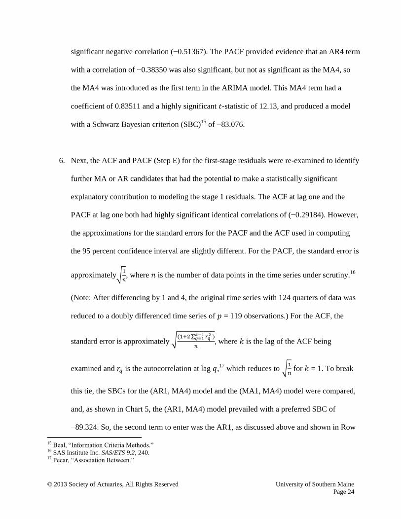
significant negative correlation (−0.51367). The PACF provided evidence that an AR4 term
with a correlation of −0.38350 was also significant, but not as significant as the MA4, so
the MA4 was introduced as the first term in the ARIMA model. This MA4 term had a
coefficient of 0.83511 and a highly significant -statistic of 12.13, and produced a model
with a Schwarz Bayesian criterion (SBC)15
of −83.076.
6. Next, the ACF and PACF (Step E) for the first-stage residuals were re-examined to identify
further MA or AR candidates that had the potential to make a statistically significant
explanatory contribution to modeling the stage 1 residuals. The ACF at lag one and the
PACF at lag one both had highly significant identical correlations of (−0.29184). However,
the approximations for the standard errors for the PACF and the ACF used in computing
the 95 percent confidence interval are slightly different. For the PACF, the standard error is
approximately
, where is the number of data points in the time series under scrutiny.
16
(Note: After differencing by 1 and 4, the original time series with 124 quarters of data was
reduced to a doubly differenced time series of = 119 observations.) For the ACF, the
standard error is approximately
where is the lag of the ACF being
examined and is the autocorrelation at lag ,17
which reduces to
for = 1. To break
this tie, the SBCs for the (AR1, MA4) model and the (MA1, MA4) model were compared,
and, as shown in Chart 5, the (AR1, MA4) model prevailed with a preferred SBC of
−89.324. So, the second term to enter was the AR1, as discussed above and shown in Row
15
Beal, “Information Criteria Methods.” 16
SAS Institute Inc. SAS/ETS 9.2, 240. 17
Pecar, “Association Between.”

© 2013 Society of Actuaries, All Rights Reserved University of Southern Maine
Page 25
2 of the Chart 5. Note that the selection of the AR1 term over the MA1 term had a
substantial impact on the quality of the model. While the PACF(1) spike and the ACF(1)
spike were identical in terms of their significance levels, the positive impact of adding the
AR1 to the initial MA4 term was clearly much greater, as reflected by the magnitude of the
-statistics for their coefficients (i.e., 3.38 vs. 1.93, respectively). Lastly, the -statistics for
the MA4 term in the two models are very different (i.e., 11.39 in Row 2 vs. 5.31 in Row 3),
and reflect the enhancing role of the AR1 term and the detracting role of the MA1 on the
MA4-foundation term common to both models. Further, the introduction of the AR1 term
only decreased the MA4 -statistic by 1.22, from 12.61 to 11.39. In contrast, adding the
MA1 to the MA4-foundation model reduced the MA4 -statistic by 7.30, from 12.61 to
5.31. This is not surprising because the lag 4 error terms were bound to capture much of the
explanatory value that the lag 1 error terms would have captured in isolation. (Note: The
correlation between MA4 and MA1 was 0.428, while the [AR1, MA4] correlation was
about two times less at 0.196.)
Chart 5. ARIMA model-building results.
Row # Model SBC Term Coefficient t Pr > |t|
1 MA4 −84.027 MA4 0.84565 12.61 <.0001
2
AR1, MA4
−89.324
AR1 −0.30254 −3.38 0.0007
MA4 0.80895 11.39 <0.0001
3
MA1, MA4
−86.402
MA1 0.28010 1.93 0.0536
MA4 0.71989 5.31 <0.0001
7. A two-stage re-examination of the ACF and PACF (Step E) of the (AR1, MA4) model’s
residuals suggested that first an AR10 term, and then an AR3 term should be added.
© 2013 Society of Actuaries, All Rights Reserved University of Southern Maine
Page 26
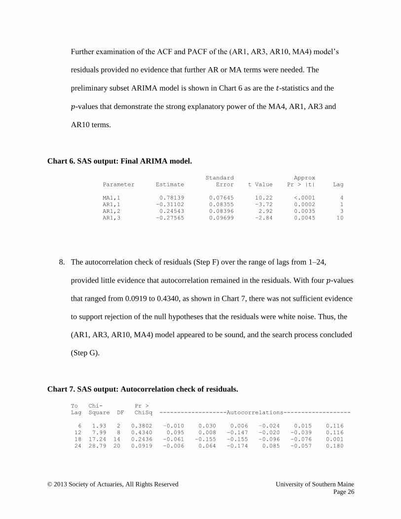
Further examination of the ACF and PACF of the (AR1, AR3, AR10, MA4) model’s
residuals provided no evidence that further AR or MA terms were needed. The
preliminary subset ARIMA model is shown in Chart 6 as are the -statistics and the
-values that demonstrate the strong explanatory power of the MA4, AR1, AR3 and
AR10 terms.
Chart 6. SAS output: Final ARIMA model.
Standard Approx
Parameter Estimate Error t Value Pr > |t| Lag
MA1,1 0.78139 0.07645 10.22 <.0001 4
AR1,1 −0.31102 0.08355 −3.72 0.0002 1
AR1,2 0.24543 0.08396 2.92 0.0035 3
AR1,3 −0.27565 0.09699 −2.84 0.0045 10
8. The autocorrelation check of residuals (Step F) over the range of lags from 1–24,
provided little evidence that autocorrelation remained in the residuals. With four -values
that ranged from 0.0919 to 0.4340, as shown in Chart 7, there was not sufficient evidence
to support rejection of the null hypotheses that the residuals were white noise. Thus, the
(AR1, AR3, AR10, MA4) model appeared to be sound, and the search process concluded
(Step G).
Chart 7. SAS output: Autocorrelation check of residuals.
To Chi- Pr >
Lag Square DF ChiSq -------------------Autocorrelations-------------------
6 1.93 2 0.3802 −0.010 0.030 0.006 −0.024 0.015 0.116
12 7.99 8 0.4340 0.095 0.008 −0.147 −0.020 −0.039 0.116
18 17.24 14 0.2436 −0.061 −0.155 −0.155 −0.096 −0.076 0.001
24 28.79 20 0.0919 −0.006 0.064 −0.174 0.085 −0.057 0.180

© 2013 Society of Actuaries, All Rights Reserved University of Southern Maine
Page 27
9. In addition to performing the diagnostic Ljung-Box test to check for independence of the
residuals, there are two other assumptions relating to residuals that must be validated:
normality and homoscedasticity.18
Normality. The residuals should be normally distributed so that the -statistics
used to assess the significance of AR and MA terms are valid. A test often used
for this purpose is the Kolmogorov-Smirnov (K-S) test,19
which examines
goodness of fit and the maximum difference between the observed cumulative
distribution function (CDF) and a fully specified hypothesized cumulative
distribution. As the vertical distance between the two CDFs increases, the K-S
statistic also increases, which discourages acceptance of the null hypothesis of
normally distributed errors. In practice, the mean and standard deviation of the
hypothesized normal cumulative distribution function are often estimated from
the sample data set,20
resulting in conservatively approximated, rather than exact,
-values.
18
Yurekli and Kurunc, “Testing the Residuals.” 19
National Institute of Standards and Technology, “Kolmogorov-Smirnov.” 20
SAS Institute Inc. “Tests for Normality.”

© 2013 Society of Actuaries, All Rights Reserved University of Southern Maine
Page 28
Figure 7. Normal probability plot of residuals.
0.500.250.00-0.25-0.50
99.9
99
95
90
80
70
605040
30
20
10
5
1
0.1
Residual: Actual-Forecast
Percen
t
Mean 0.005901
StDev 0.1502
N 119
KS 0.048
P-Value >0.150
In the Minitab-generated Figure 7 constructed with the 119 residuals from the
(AR1, AR3, AR10, MA4) fitted model, the K-S statistic is 0.048 with an
attractive estimated -value of >0.150 for the N(0.005901, 0.1502) fitted
distribution. This does not support rejection of the null hypothesis that the (AR1,
AR3, AR10, MA4) model residuals are normally distributed. The average of the
119 residuals is close to zero (0.005901) and the standard error (S.E.) =
StDev/ = 0.1502/ = 0.0138. As such, the mean of the residuals is not
statistically different from zero since Z = – S.E. = [0.005901 – 0]/0.0138
= 0.427.
© 2013 Society of Actuaries, All Rights Reserved University of Southern Maine
Page 29
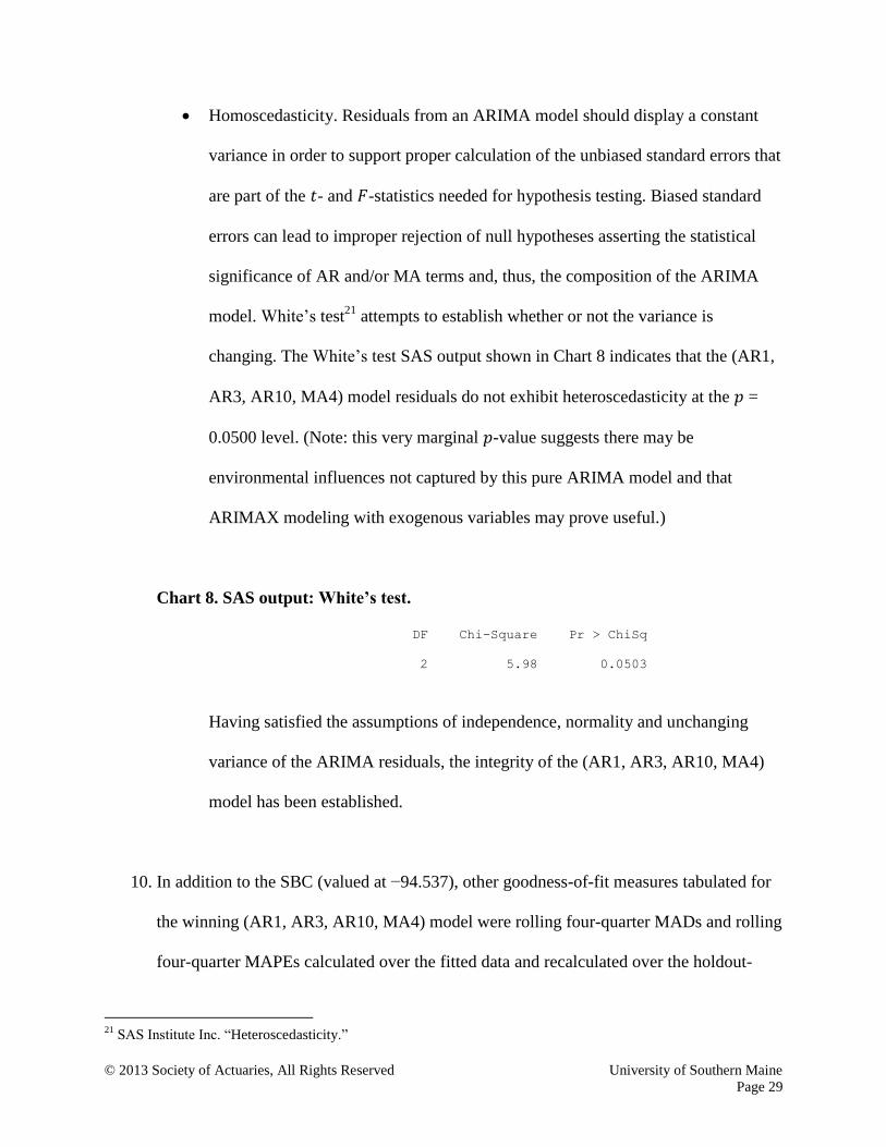
Homoscedasticity. Residuals from an ARIMA model should display a constant
variance in order to support proper calculation of the unbiased standard errors that
are part of the - and -statistics needed for hypothesis testing. Biased standard
errors can lead to improper rejection of null hypotheses asserting the statistical
significance of AR and/or MA terms and, thus, the composition of the ARIMA
model. White’s test21
attempts to establish whether or not the variance is
changing. The White’s test SAS output shown in Chart 8 indicates that the (AR1,
AR3, AR10, MA4) model residuals do not exhibit heteroscedasticity at the =
0.0500 level. (Note: this very marginal -value suggests there may be
environmental influences not captured by this pure ARIMA model and that
ARIMAX modeling with exogenous variables may prove useful.)
Chart 8. SAS output: White’s test.
DF Chi-Square Pr > ChiSq
2 5.98 0.0503
Having satisfied the assumptions of independence, normality and unchanging
variance of the ARIMA residuals, the integrity of the (AR1, AR3, AR10, MA4)
model has been established.
10. In addition to the SBC (valued at −94.537), other goodness-of-fit measures tabulated for
the winning (AR1, AR3, AR10, MA4) model were rolling four-quarter MADs and rolling
four-quarter MAPEs calculated over the fitted data and recalculated over the holdout-
21
SAS Institute Inc. “Heteroscedasticity.”
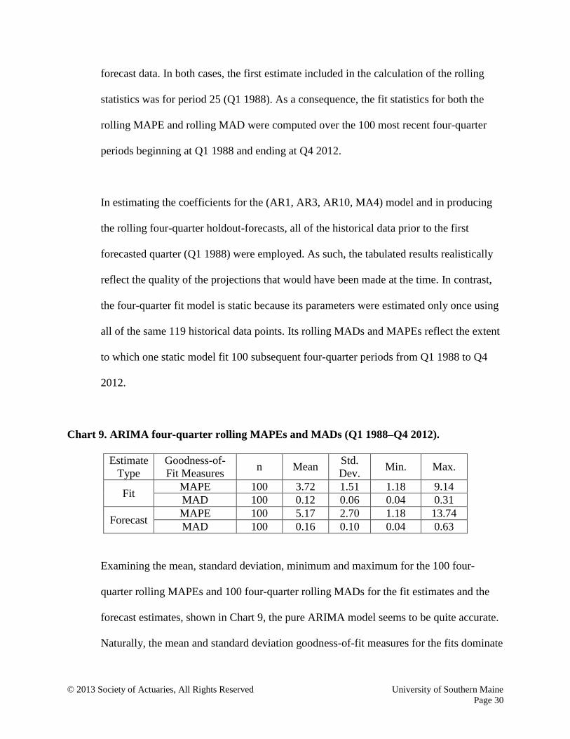
© 2013 Society of Actuaries, All Rights Reserved University of Southern Maine
Page 30
forecast data. In both cases, the first estimate included in the calculation of the rolling
statistics was for period 25 (Q1 1988). As a consequence, the fit statistics for both the
rolling MAPE and rolling MAD were computed over the 100 most recent four-quarter
periods beginning at Q1 1988 and ending at Q4 2012.
In estimating the coefficients for the (AR1, AR3, AR10, MA4) model and in producing
the rolling four-quarter holdout-forecasts, all of the historical data prior to the first
forecasted quarter (Q1 1988) were employed. As such, the tabulated results realistically
reflect the quality of the projections that would have been made at the time. In contrast,
the four-quarter fit model is static because its parameters were estimated only once using
all of the same 119 historical data points. Its rolling MADs and MAPEs reflect the extent
to which one static model fit 100 subsequent four-quarter periods from Q1 1988 to Q4
2012.
Chart 9. ARIMA four-quarter rolling MAPEs and MADs (Q1 1988–Q4 2012).
Estimate
Type
Goodness-of-
Fit Measures n Mean
Std.
Dev. Min. Max.
Fit MAPE 100 3.72 1.51 1.18 9.14
MAD 100 0.12 0.06 0.04 0.31
Forecast MAPE 100 5.17 2.70 1.18 13.74
MAD 100 0.16 0.10 0.04 0.63
Examining the mean, standard deviation, minimum and maximum for the 100 four-
quarter rolling MAPEs and 100 four-quarter rolling MADs for the fit estimates and the
forecast estimates, shown in Chart 9, the pure ARIMA model seems to be quite accurate.
Naturally, the mean and standard deviation goodness-of-fit measures for the fits dominate
© 2013 Society of Actuaries, All Rights Reserved University of Southern Maine
Page 31
their counterparts from the holdout forecasts. In both cases, however, the mean four-
quarter rolling MADs of 0.12 and 0.16 are quite respectable in relation to the range of the
raw time-series values (1.93–5.29) over the 25-year period. The rolling MAPEs averaged
3.72 percent for the fit model and 5.17 percent for the forecast model over the same 25
years.
All of these goodness-of-fit statistics are quite attractive given the substantial expanse of
the time period, as well as the dynamics of the economy and the evolution of SSA’s
policies/persuasions. After all, this forecasting methodology relies only on historical
time-series patterns to make its projections, and has no mechanisms for directly
integrating the impacts of exogenous influences. Addressing this deficit is the topic of
Section 2.2.

© 2013 Society of Actuaries, All Rights Reserved University of Southern Maine
Page 32
2.2 Construction and Validation of an ARIMAX Model
ARIMAX is an acronym for autoregressive integrated moving-average with exogenous
variables. It is a logical extension of pure ARIMA modeling that incorporates independent
variables which add explanatory value. Conceptually, it is a merging of regression and ARIMA
modeling.22
When the AR and MA terms in a pure ARIMA model are not sufficient to provide
an acceptably high (or some other measure of a model’s overall explanatory power), it is only
natural to look for other driving phenomena whose influence over time is not sufficiently
embedded in the historical values of the dependent time series.
Building an ARIMAX model calls for combining the predictive value of both the trailing time-
series values themselves ( ) and the trailing model errors ( ) with the predictive value of
exogenous variables. As a simple example, if a set of exogenous variables serving as
independent variables in a multiple regression were all properly signed and highly significant,
did not exhibit significant cross-correlation and produced a high with the time series of
residuals approximating white noise, there would be no need for ARIMAX modeling. However,
if that same multivariate regression equation generated residuals that exhibited significant serial
correlation, then pure ARIMA modeling of the residuals would be required in order to remove
the serial correlation so that -statistics could be properly calculated and the significance of the
independent variables could be properly judged.
The ARIMAX approach to time-series model building has two phases. This methodology
traditionally begins with a logically attractive and statistically sound regression model. Then, the
22
SAS Institute Inc. SAS/ETS 9.2, 21.3

© 2013 Society of Actuaries, All Rights Reserved University of Southern Maine
Page 33
errors from the regression are modeled with AR and MA terms to remove any statistically
significant serial correlation that remains in the residual time series. (Note: The final ARIMAX
model is composed of exogenous variables along with AR and/or MA terms, so it is sometimes
useful to conduct an exploration for exogenous terms using the residuals from a pure ARIMA
and then look at their cross-correlations with other explanatory variables.23
This is particularly
true if the pure ARIMA is stable and it explains the vast majority of the variation of the
dependent variable. After all, it is the exogenous, AR and MA terms that collectively comprise
the final model, and they need to complement each other to maximize the explanatory power of
the RHS variables while eliminating any significant autocorrelation among the residuals.)
While the traditional (regression-first) two-phase process appears to be straightforward, it is not.
There is a powerful interaction created by the integration of AR and MA terms into a multiple
regression model that frequently creates the need for an iterative search process. This is
particularly true if the pool of exogenous-variable candidates is large. For example, when a new
exogenous variable is selected in a stepwise process and introduced to the ARIMAX model, it
may well disrupt the white-noise pattern of the residuals from the previous step. This concern
would need to be addressed with the addition of new AR and/or MA terms to re-establish the
random pattern of residuals. In turn, the newly added AR and/or MA terms may explain variation
previously explained by one or more resident exogenous variables, which then forces one or more
of these impacted independent variables out of the ARIMAX model. This disruption, in turn,
produces new residuals whose ACF and PACF must be examined to determine if additional AR
or MA terms should be added to the model. Once the serial correlation is removed, additional
23
Nau, “ARIMA Models.”
© 2013 Society of Actuaries, All Rights Reserved University of Southern Maine
Page 34
exogenous variables may need to be removed due to lack of significance, and so the cycle
continues.
There are six statistical assumptions that must be examined/re-examined to ensure that the
resulting ARIMAX model is valid at each stage of its evolution. Two of these six assumptions
(denoted as assumptions 1 and 2) pertain to the residuals produced by the model, and the other
four (denoted as assumptions 3–6) relate to the exogenous variables that comprise the model.
Assumption 1. As discussed in Section 2.1, ARIMA model building may not commence until
the time series is stationary.24
This requires that the mean and the variance of the residual
series are unchanging over time. The degree of stationarity of the residuals may be
statistically evaluated using the augmented Dickey-Fuller test.25
As before with pure ARIMA
model building, the -values for the augmented Dickey-Fuller test for a single mean must be
acceptably small to ensure stationarity. If the residuals produced by the regression are not
sufficiently stationary, the level of stationarity may oftentimes be improved by applying the
same well-chosen differencing scheme (or another transformation) to the dependent and to all
of the exogenous variables.
Assumption 2. In addition to stationarity, the residual series must not exhibit significant
serial correlation (i.e., autocorrelation). The Ljung-Box test may be used to statistically
evaluate the degree to which the residuals are serially correlated. If significant serial
correlation exists among the residuals, it may be reduced by adding an appropriate
24
SAS Institute Inc. SAS/ETS 9.2, 215. 25
Ibid.,158.

© 2013 Society of Actuaries, All Rights Reserved University of Southern Maine
Page 35
combination of one or more significant AR and/or MA terms identified from the PACF and
ACF, respectively.
Assumption 3. The estimated coefficient for an exogenous variable must be significantly
different than 0, as judged by its -statistic. However, the calculation of the significance
levels of -statistics ( -values) for regression coefficients assumes that the regression
residuals are white noise. If Assumption 2 is violated, and these residuals are not white noise,
then their serial correlation must be removed with ARIMA modeling. This calls for the pure
ARIMA modeling process discussed in Section 2.1 and outlined in Figure 4.
Assumption 4. An exogenous variable must not display evidence of receiving feedback from
the dependent variable. That is, an attractive exogenous-variable candidate should display a
significant causal relationship with the dependent variable without the dependent variable
displaying a causal relationship with it. The directions of significant causality between an
exogenous variable and the dependent variable may be tested using the Granger causality
test26
. If reverse causality is detected, the exogenous variable must be removed from the pool
of independent-variable candidates. This test must be performed on the dependent and
independent variable in their current form (untransformed or transformed).
Assumption 5. The sign of the coefficient for each significant exogenous variable must be
reasonable. The expected (i.e., reasonable) sign can be determined prior to model building by
examining the signs of exogenous-variable correlation-coefficients that display a significant
26
SAS Institute Inc. “Bivariate Granger.”
© 2013 Society of Actuaries, All Rights Reserved University of Southern Maine
Page 36
correlation with the dependent variable. If the dependent variable required a transformation
to achieve stationarity, that same transformation would also be applied to the independent-
variable candidates, and the bivariate-correlation analysis would then focus on the pair of
transformed variables.
Assumption 6. The surviving exogenous variables comprising the final model must not
exhibit a significant degree of multicollinearity. To meet this condition, one at a time, each of
the surviving exogenous variables must be individually tested for significant multicollinearity
using the variance inflation factor (VIF = ]) to ensure they are all sufficiently
linearly independent. When the multicollinearity among exogenous variables is too strong,
least squares estimation becomes inefficient, causing the standard errors of the estimates to
become large and result in overstated -values. A VIF of 10 or less is generally considered to
indicate an acceptable level of correlation among the exogenous variables. The VIF
calculations must be performed for each of the independent variables expressed in their
current form (i.e., transformed or untransformed). (Note: Each of the s is actually
calculated by selecting one of the independent variables to assume the role of dependent
variable in a regression with all of the remaining independent variables serving as
independent variables.) Thus, the VIF ≤ 10 rule of thumb is the equivalent of requiring that
each independent variable’s variation be no more than 90 percent explainable based on the
weighted aggregate of the other independent variables.
© 2013 Society of Actuaries, All Rights Reserved University of Southern Maine
Page 37
The flowchart shown in Figure 8 presents the algorithm used to build a valid ARIMAX model. It
is constructed using an iterative scheme based largely on the principles embodied in the six
assumptions above. As indicated by the maze of 40 nested and unnested looping structures, the
examination/re-examination of assumptions 1–6 provides the foundation for the model-building
methodology. Excluding the A. Start and the R. Stop nodes, there are 16 steps, many of which are
executed numerous times. The five core steps (B–F) in the ARIMA model-building algorithm
presented earlier are also embedded in this flowchart. The substantial increase in steps from 5 to
16 is largely based on the complexities introduced by marrying the elements/requirements of
regression model building with those of the pure-ARIMA model building.

© 2013 Society of Actuaries, All Rights Reserved University of Southern Maine
Page 38
Figure 8. ARIMAX model-building algorithm.

© 2013 Society of Actuaries, All Rights Reserved University of Southern Maine
Page 39
There are three families of looping structures labeled B, H and I, with two B-loops, six H-loops and
two I-loops. Note that the six H-loops are nested inside the B2 loop and the two I-loops both are
nested inside all six H-loops. This creates 40 loops in total: 10 unnested, 18 singly nested and 12
doubly nested.
B-loops:
1. BCB
2. BD E F G H C B
H-loops:
1. H I K L H
2. H I J K L H
3. H I K M N H
4. H I J K M N H
5. H I K M O P H
6. H I J K M O P H
I-loops:
1. I K M O Q I
2. I J K M O Q I
One of the early tasks of ARIMAX model building is to identify and preliminarily evaluate the
logical/statistical attractiveness of exogenous variable candidates. SSDI application rates have been
well studied over the years, so for this study, there was no shortage of attractive explanatory-variable
candidates. The U.S. Social Security Administration website has a wealth of literature on this topic,
most of which relates to the condition of the U.S. economy. For this model-building exercise, 14
exogenous-variable candidates were identified. Expecting that these 14 exogenous variables might

© 2013 Society of Actuaries, All Rights Reserved University of Southern Maine
Page 40
lead quarterly SSDI application rates, each of 14 candidates was assigned to lags of 0, 1, 2, 3 and 4
quarters, thus creating 70 independent-variable candidates in total. Chart 10 provides each variable’s
name, description and data source.
Chart 10. 70 Exogenous-variable candidates.
SAS Variable
(Each With Lags
0–4)
Description
Source
total_permits total single and multifamily permits Moody’s Analytics
housing_starts housing starts (in millions) Moody’s Analytics
median_home_price median single-family home price
(in thousands)
Moody’s Analytics
total_fixed_invest total fixed investment (in billions
of 2005 dollars)
Moody’s Analytics
wse number of nonfarm, payroll jobs in
the U.S economy (in thousands)
bls.gov/data: Employment;
Employment, Hours, and Earnings—
National (Current Employment
Statistics)
resident_employment number employed (in thousands) bls.gov/data: Employment; Labor
Force Statistics (Current Population
Survey)
unemployment unemployment rate bls.gov/data: Unemployment; Labor
Force Statistics (Current Population
Survey)
num_unemployed number unemployed (in thousands) bls.gov/data: Unemployment; Labor
Force Statistics (Current Population
Survey)
cpi_urban Consumer Price Index for all urban
consumers – all items
bls.gov/data: Inflation & Prices; All
Urban Consumers (Consumer Price
Index)
nom_gdp GDP (in billions of current dollars) bea.gov/national/index.htm:
Current-dollar and “real” GDP
real_gdp GDP (in billions of 2005 dollars) bea.gov/national/index.htm:
Current-dollar and “real” GDP
mean_earnings mean individual weekly earnings Moody’s Analytics
weekly_hours average number of weekly hours:
total nonfarm
Moody’s Analytics
hourly_earnings average hourly earnings: total
nonfarm
Moody’s Analytics
Lagged (1–4) forms for exogenous variables are denoted with suffixes.

© 2013 Society of Actuaries, All Rights Reserved University of Southern Maine
Page 41
Building an ARIMAX model requires executing some combination of the 16 (or fewer) steps in
Figure 8, the ARIMAX model-building flowchart.
1. As in the pure ARIMA model-building process discussed earlier, the first two steps
involve testing the dependent time series for stationarity using the augmented Dickey-
Fuller test (Step B) and, if required, selecting an appropriate differencing scheme for the
dependent variable (Step C).
2. Frequently, for consistency, the differencing scheme chosen for the dependent variable
during pure ARIMA model building can be applied to exogenous-variable candidates to
make them stationary as well. With both the dependent and independent variables
stationary, the correlations are more likely to be stable over time.27
In this case, all of the
exogenous-variable candidates became stationary after being differenced by 1 and 4.
Note that these transformations must be performed at an early stage in the model-building
process so that subsequent tests such as the Granger test of causality will employ the
exogenous variables in the form they will subsequently appear in the final model.
3. Next, the transformed exogenous variables are screened using the Granger test for
causality (Step E) to remove any variables that display significant evidence of reverse
causality, as discussed above in Assumption 4. Any variable with a -value below 0.0500
led to rejection of the null hypothesis of no reverse causality, thus eliminating it as a
candidate for inclusion in the model. This reduced the pool of exogenous-variable
27 Nau, “Identifying the Numbers.”

© 2013 Society of Actuaries, All Rights Reserved University of Southern Maine
Page 42
candidates from 70 to 57. The 13 eliminated variables and their associated -values are
shown in Chart 11.
Chart 11. Exogenous-variable candidates eliminated by Granger test for causality.
Variable_Name Chi-Square Pr > ChiSq
wse_3 10.08 0.0015
wse_1 9.24 0.0024
mean_earnings_2 8.42 0.0037
total_fixed_invest_3 7.15 0.0075
unemployment_2 6.76 0.0093
real_gdp_2 6.42 0.0113
num_unemployed_2 6.41 0.0114
weekly_hours_2 6.40 0.0114
total_fixed_invest_1 6.37 0.0116
cpi_urban_1 6.19 0.0128
nom_gdp_2 5.73 0.0167
resident_employment 5.02 0.0251
median_home_price_1 4.79 0.0286
4. As previously discussed in Assumption 5, the “correct” signs for the remaining
transformed exogenous-variable candidates (Step F) must be determined by performing
an analysis of the correlations between the transformed exogenous-variable candidates
and the transformed dependent variable. Variables that do not display a significant
correlation ( < 0.0500) are not assigned an expected sign and are removed from the pool
of independent-variable candidates. Chart 12 presents the 14 surviving
exogenous-variable candidates, their correlation coefficients and their corresponding
-values. (Note: Since SAS employs a two-tailed test of significance for correlation
coefficients, the -value threshold of 0.1000 was employed.)
© 2013 Society of Actuaries, All Rights Reserved University of Southern Maine
Page 43
Chart 12. Exogenous-variable candidates remaining after correlation analysis.
Exogenous Variable Corr. Coef. -value
wse −0.31133 0.0007
total_fixed_invest −0.27009 0.0035
cpi_urban −0.25722 0.0055
real_gdp_1 −0.25392 0.0062
nom_gdp −0.24711 0.0078
nom_gdp_1 −0.23703 0.0108
unemployment_1 0.22976 0.0135
num_unemployed_1 0.22806 0.0142
weekly_hours_1 −0.20689 0.0265
mean_earnings_1 −0.20241 0.0300
median_home_price −0.17641 0.0593
num_unemployed 0.17640 0.0593
real_gdp −0.17133 0.0671
cpi_urban_4 0.16875 0.0714
The signs of these 14 significant correlation coefficients are retained for subsequent use
in Step O to eliminate from the ARIMAX model any of the significant exogenous
variables whose coefficients are incorrectly signed.
5. The forward/backward stepwise regression procedure in SAS provides an iterative
approach to regression model building that both adds significant variables to the model
and removes variables from the model that become insignificant (Step G). The process
begins by determining the exogenous-variable candidate with the smallest -value that is
less than the chosen “enter” significance-level threshold of 0.1000 and adding that
variable to the model. Next, the -values of all of the variables in the current model are
checked, and the variable with the largest -value above the chosen “stay” significance-
level threshold of 0.0500 is removed. This process of adding and deleting exogenous

© 2013 Society of Actuaries, All Rights Reserved University of Southern Maine
Page 44
variables continues until there are no variables that meet either criterion.28
The final
results of the three iterations of the stepwise process are displayed in the SAS output of
Chart 13.
Chart 13. SAS output: Summary of stepwise selection.
Variable Variable Number Partial Model
Step Entered Removed Vars In R-Square R-Square C(p) F Value Pr > F
1 wse 1 0.0968 0.0968 0.8865 12.22 0.0007
2 num_unemployed 2 0.0238 0.1206 −0.1150 3.06 0.0830
3 num_unemployed 1 0.0238 0.0968 0.8865 3.06 0.0830
As shown in the SAS output in Chart 14, the final iteration of the stepwise-regression
process results in a standard regression model containing one exogenous variable, which
is highly significant (with a -value of 0.0007).
Chart 14. SAS output: Stepwise-regression parameter estimates.
Parameter Standard Variance
Variable DF Estimate Error t Value Pr > |t| Inflation
wse 1 −0.00011108 0.00003177 −3.50 0.0007 1.00000
6. The significance level of this independent-variable coefficient is calculated under the
assumption that the residuals simulate white noise. To properly make these assessments,
the residuals must be tested first for stationarity and then for serial correlation. As shown
in Chart 15, with -values <.0001 for all five lags, the augmented Dickey-Fuller test
results provide strong evidence that the residuals of the regression are stationary (Step H).
28
Beal, “Information Criteria Methods.”
© 2013 Society of Actuaries, All Rights Reserved University of Southern Maine
Page 45
Chart 15. SAS output: Augmented Dickey-Fuller test.
Type Lags Pr < Tau
Single Mean 0 <.0001
1 <.0001
2 <.0001
3 <.0001
4 <.0001
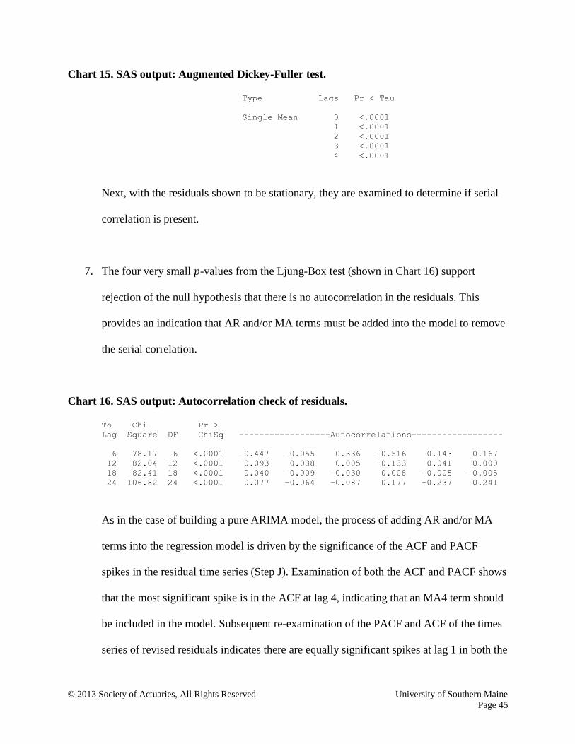
Next, with the residuals shown to be stationary, they are examined to determine if serial
correlation is present.
7. The four very small -values from the Ljung-Box test (shown in Chart 16) support
rejection of the null hypothesis that there is no autocorrelation in the residuals. This
provides an indication that AR and/or MA terms must be added into the model to remove
the serial correlation.
Chart 16. SAS output: Autocorrelation check of residuals.
To Chi- Pr >
Lag Square DF ChiSq ------------------Autocorrelations------------------
6 78.17 6 <.0001 −0.447 −0.055 0.336 −0.516 0.143 0.167
12 82.04 12 <.0001 −0.093 0.038 0.005 −0.133 0.041 0.000
18 82.41 18 <.0001 0.040 −0.009 −0.030 0.008 −0.005 −0.005
24 106.82 24 <.0001 0.077 −0.064 −0.087 0.177 −0.237 0.241
As in the case of building a pure ARIMA model, the process of adding AR and/or MA
terms into the regression model is driven by the significance of the ACF and PACF
spikes in the residual time series (Step J). Examination of both the ACF and PACF shows
that the most significant spike is in the ACF at lag 4, indicating that an MA4 term should
be included in the model. Subsequent re-examination of the PACF and ACF of the times
series of revised residuals indicates there are equally significant spikes at lag 1 in both the

© 2013 Society of Actuaries, All Rights Reserved University of Southern Maine
Page 46
ACF and the PACF. Consistent with the tie-breaking logic previously employed in
building the pure ARIMA model, the SBCs are examined for both models. As shown in
rows 2 and 3 of Chart 17, introducing an MA1 term into the model produces an SBC of
−101.6, while introducing an AR1 term instead produces a more attractive SBC of
−108.315. Additionally, the correlation between the MA1 and MA4 terms is 0.473, while
the correlation between AR1 and MA4 is only 0.207. This explains the mitigating impact
that including an MA1 term has on the -statistic of the MA4 term, reducing it from
11.64 to 4.38. In contrast, introducing an AR1 term instead of the MA1 term only
decreases the MA4 -statistic slightly from 11.64 to 10.47.
Chart 17. ARIMAX model-building results.
Row # Model SBC Term Coefficient Pr >
1 MA4 −90.1125 MA4 0.82916 11.64 <.0001
2
AR1, MA4
−108.315
AR1 −0.42587 −4.99 <.0001
MA4 0.79019 10.47 <.0001
3
MA1, MA4
−101.6
MA1 0.39005 2.39 0.0168
MA4 0.60995 4.38 <.0001
Examination of the ACF and PACF shows there is a significant spike in the PACF at lag
2, indicating that an AR2 term should be included in the model. Further examination of
the ACF and PACF indicates there are no other significant spikes.
8. After the significant ( < 0.05) AR1, AR2 and MA4 terms are entered, it is necessary to
ensure that the exogenous variable(s) in the model remain significant (Step K). The

© 2013 Society of Actuaries, All Rights Reserved University of Southern Maine
Page 47
variable is still significant ( -value <.0001 indicated in Chart 18) and can remain in
the model.
Chart 18. SAS output: ARIMAX model.
Parameter Estimate StdErr tValue Probt Lag Variable
AR1,2 −0.2484659 0.09007034 −2.76 0.0058 2 adj_rate
AR1,1 −0.5266464 0.09091027 −5.79 <.0001 1 adj_rate
NUM1 −0.0000842 0.00001235 −6.82 <.0001 0 wse
MA1,1 0.79784551 0.07491641 10.65 <.0001 4 adj_rate
9. Because there is only one exogenous variable present in the model, multicollinearity is
not a concern (Step M). The SAS output is shown in Chart 19.
Chart 19. SAS output: Exogenous-variable multicollinearity check.
Parameter Standard Variance
Variable Label DF Estimate Error t Value Pr > |t| Inflation
wse wse 1 −0.00009432 0.00002953 −3.19 0.0018 1.00000
10. The sign check (Step O) ensures the remaining exogenous variable has a proper sign that
matches what was determined by the correlation analysis in Step F, as shown in Chart 20.
Chart 20. SAS output: Exogenous-variable sign check.
Parameter Standard
Pearson
Correlation Sign
Variable Estimate Error Coefficient Check
wse −0.00009432 0.00002953 −0.31133 Pass
11. Lastly, all of the -values from the Ljung-Box test are sufficiently large (ranging from
0.1946 to 0.5857 as indicated in Chart 21), indicating that the null hypothesis of white
noise residuals should not be rejected (Step Q).
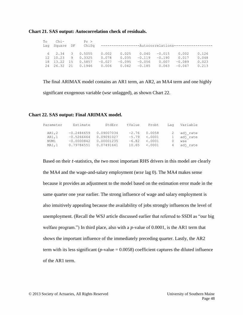
© 2013 Society of Actuaries, All Rights Reserved University of Southern Maine
Page 48
Chart 21. SAS output: Autocorrelation check of residuals.
To Chi- Pr >
Lag Square DF ChiSq ------------------Autocorrelations------------------
6 2.34 3 0.5055 0.002 0.025 0.040 −0.015 0.002 0.126
12 10.23 9 0.3325 0.078 0.035 −0.119 −0.190 0.017 0.048
18 13.22 15 0.5857 −0.027 −0.095 −0.056 0.007 −0.089 0.023
24 26.32 21 0.1946 0.006 0.042 −0.185 0.063 −0.047 0.213
The final ARIMAX model contains an AR1 term, an AR2, an MA4 term and one highly
significant exogenous variable (wse unlagged), as shown Chart 22.
Chart 22. SAS output: Final ARIMAX model.
Parameter Estimate StdErr tValue Probt Lag Variable
AR1,2 −0.2484659 0.09007034 −2.76 0.0058 2 adj_rate
AR1,1 −0.5266464 0.09091027 −5.79 <.0001 1 adj_rate
NUM1 −0.0000842 0.00001235 −6.82 <.0001 0 wse
MA1,1 0.79784551 0.07491641 10.65 <.0001 4 adj_rate
Based on their -statistics, the two most important RHS drivers in this model are clearly
the MA4 and the wage-and-salary employment ( lag 0). The MA4 makes sense
because it provides an adjustment to the model based on the estimation error made in the
same quarter one year earlier. The strong influence of wage and salary employment is
also intuitively appealing because the availability of jobs strongly influences the level of
unemployment. (Recall the WSJ article discussed earlier that referred to SSDI as “our big
welfare program.”) In third place, also with a -value of 0.0001, is the AR1 term that
shows the important influence of the immediately preceding quarter. Lastly, the AR2
term with its less significant ( -value = 0.0058) coefficient captures the diluted influence
of the AR1 term.

© 2013 Society of Actuaries, All Rights Reserved University of Southern Maine
Page 49
12. As in the case of the pure ARIMA model, it is necessary to ensure that the residuals of
the ARIMAX model satisfy the conditions of normality and homoscedasticity. The
Kolmogorov-Smirnov (K-S) test on the 119 residuals from the ARIMAX model yields a
K-S statistic of 0.069 with a -value of >0.150, which does not support rejection of the
null hypothesis of normally distributed residuals (see Figure 9).
Figure 9. Normal probability plot of residuals.
0.500.250.00-0.25-0.50
99.9
99
95
90
80
70
605040
30
20
10
5
1
0.1
Residual: Actual-Forecast
Percen
t
Mean 0.004823
StDev 0.1421
N 119
KS 0.069
P-Value >0.150
In addition, White’s test, with a -value of 0.2043, indicates that the null hypothesis of
homoscedasticity cannot be rejected (see Chart 23).

© 2013 Society of Actuaries, All Rights Reserved University of Southern Maine
Page 50
Chart 23. SAS output: White’s test.
DF Chi-Square Pr > ChiSq
2 3.18 0.2043
13. The SBC (−110.996) of the ARIMAX model (with its additional SBC-penalizing
exogenous variable and additional AR2 term) is more attractive than that of the pure
ARIMA model (−94.537). It is also useful to examine the goodness-of-fit measures such
as the MAD and MAPE for the new ARIMAX model and to compare them to those of
the pure ARIMA model to help evaluate the improved precision of the ARIMAX model.
As before with the pure ARIMA model, the four-quarter rolling MAPEs and MADs were also
tabulated for the ARIMAX fit and forecast models. Unsurprisingly, the fits again outperform the
holdout forecasts, although both show quite impressive goodness-of-fit results (see Chart 24).
Chart 24. ARIMAX four-quarter rolling MAPEs and MADs (Q1 1988–Q4 2012).
Estimate
Type
Goodness-of-
Fit Measures n Mean
Std.
Dev. Min. Max.
Fit MAPE 100 3.20 1.62 0.79 9.14
MAD 100 0.10 0.06 0.02 0.32
Forecast MAPE 100 4.06 2.24 0.62 12.07
MAD 100 0.12 0.07 0.02 0.37
As seen in the performance comparison displayed in Chart 25, the ARIMAX model’s average
four-quarter rolling fit and forecast MAPEs show improvement at 3.20 percent and 4.06 percent,
when compared to the pure ARIMA model’s 3.72 percent and 5.17 percent, respectively.
Further, the ARIMAX model’s four-quarter rolling MADs for the fit and forecast models
averaged 0.10 and 0.12, respectively, which is an attractive relative improvement over their

© 2013 Society of Actuaries, All Rights Reserved University of Southern Maine
Page 51
counterparts in the pure ARIMA model (0.12 and 0.16). In fact, when comparing the four-quarter
rolling MAPEs and MADs for the forecast and fit estimates, the ARIMAX model is preferable to
the ARIMA model in almost every way, with its generally lower means, standard deviations,
minimums and maximums (as seen by the ARIMAX/ARIMA ratios). In Chart 25, all but two of
the 16 MAPE and MAD ARIMAX/ARIMA ratios for the means are less than or equal to one.
Chart 25. Performance comparison of ARIMA and ARIMAX models:
Four-quarter rolling MAPEs and MADs (100 quarters: Q1 1988–Q4 2012).
Estimate
Type
Goodness-of-
Fit Measures Model Mean
Std.
Dev. Min. Max.
FIT
MAPE
ARIMA 3.72 1.51 1.18 9.14
ARIMAX 3.20 1.62 0.79 9.14
ARIMAX/ARIMA 0.86 1.07 0.67 1.00
MAD
ARIMA 0.12 0.06 0.04 0.31
ARIMAX 0.10 0.06 0.02 0.32
ARIMAX/ARIMA 0.83 1.00 0.50 1.03
FORECAST
MAPE
ARIMA 5.17 2.70 1.18 13.74
ARIMAX 4.06 2.24 0.62 12.07
ARIMAX/ARIMA 0.79 0.83 0.53 0.88
MAD
ARIMA 0.16 0.10 0.04 0.63
ARIMAX 0.12 0.07 0.02 0.37
ARIMAX/ARIMA 0.75 0.70 0.50 0.59

© 2013 Society of Actuaries, All Rights Reserved University of Southern Maine
Page 52
As a further mechanism to contrast the performance of the ARIMA and ARIMAX models, time-
series graphs of the 100 four-quarter rolling MAPEs and MADs produced by the ARIMA and
ARIMAX models are provided below. These graphs serve to further confirm the benefits of
including exogenous variables in the model-building process.
Figure 10. Time-series graphs of four-quarter rolling MAPES and MADS: Produced by the
ARIMA and ARIMAX forecast and fit models (100 quarters: Q1 1988–Q4 2012).
0 1 2 3 4 5 6 7 8 9
10 11 12 13 14
1 10 19 28 37 46 55 64 73 82 91 100
FO
RE
CA
ST
MO
DE
L 4
-Qtr
RO
LL
ING
MA
PE
Quarter
ARIMA ARIMAX
0 1 2 3 4 5 6 7 8 9
10 11 12 13 14
1 10 19 28 37 46 55 64 73 82 91 100
FIT
MO
DE
L 4
-Qtr
RO
LL
ING
MA
PE
Quarter
ARIMA ARIMAX
0 0.05
0.1 0.15
0.2 0.25
0.3 0.35
0.4 0.45
0.5 0.55
0.6 0.65
1 10 19 28 37 46 55 64 73 82 91 100
FO
RE
CA
ST
MO
DE
L 4
-Qtr
RO
LL
ING
MA
D
Quarter
ARIMA ARIMAX
0 0.05
0.1 0.15
0.2 0.25
0.3 0.35
0.4 0.45
0.5 0.55
0.6 0.65
1 10 19 28 37 46 55 64 73 82 91 100
FIT
MO
DE
L 4
-Qtr
RO
LL
NG
MA
D
Quarter
ARIMA ARIMAX
© 2013 Society of Actuaries, All Rights Reserved University of Southern Maine
Page 53
REFERENCES
Beal, Dennis J. “Information Criteria Methods in SAS for Multiple Linear Regression Models.”
SA05, presented at SouthEast SAS Users Group (SESUG) Conference, Hilton Head, SC,
November 4–6, 2007. http://analytics.ncsu.edu/sesug/2007/SA05.pdf.
Brocklebank, John C., and David A. Dickey. SAS for Forecasting Time Series. 2nd
edition. Cary,
NC: SAS Institute Inc. and Wiley, 2003.
Montgomery, Douglas C., Cheryl L. Jennings, and Murat Kulahci. Introduction to Time Series
Analysis and Forecasting. Hoboken, NJ: John Wiley & Sons, Inc., 2008.
Nau, Robert F. “ARIMA Models with Regressors.” Lesson for Decision 411: Forecasting class.
Duke University, Durham, NC. May 16, 2005. http://www.duke.edu/~rnau/arimreg.htm.
———. “Fitting Time Series Regression Models.” Lesson for Decision 411: Forecasting class.
Duke University, Durham, NC. May 16, 2005. http://www.duke.edu/~rnau/411l696.htm.
———. “Identifying the Numbers of AR or MA Terms.” Lesson for Decision 411: Forecasting
class. Duke University, Durham, NC. May 16, 2005. http://www.duke.edu/~rnau/411arim3.htm.
———. “Identifying the Order of Differencing.” Lesson for Decision 411: Forecasting class.
Duke University, Durham, NC. May 16, 2005. http://www.duke.edu/~rnau/411arim2.htm.
National Institute of Standards and Technology. “Kolmogorov-Smirnov Goodness-of-Fit Test.”
NIST/SEMATECH e-Handbook of Statistical Methods, chapter 1.3.5.16.
http://www.itl.nist.gov/div898/handbook/eda/section3/eda35g.htm.
Paletta, Damian, and Dionne Searcey. “Jobless Tap Disability Fund.” The Wall Street Journal
December 28, 2011: A1.
http://online.wsj.com/article/SB10001424052970204296804577121392750460030.html.
Pecar, Branko. “Association Between and Within the Time Series.” In unpublished manuscript,
Excel Forecasting Models for Business, Finance and IT. April 2012. http://pecar-
uk.com/Autocorrelations.pdf.
SAS Institute Inc. “Bivariate Granger Causality Test.” SAS/ETS Examples. Version 9.0.
http://support.sas.com/rnd/app/examples/ets/granger/index.htm
SAS Institute Inc. Forecasting Examples: for Business and Economics Using SAS. Cary, NC:
SAS Institute Inc., 1996.
———. SAS/ETS 9.2 U r’ Guid . Cary, NC: SAS Institute Inc., 2008.
http://support.sas.com/documentation/cdl/en/etsug/60372/PDF/default/etsug.pdf.
© 2013 Society of Actuaries, All Rights Reserved University of Southern Maine
Page 54
———. SAS/ETS 9.2 U r’ Guid . Cary, NC: SAS Institute Inc., December 8, 2010.
http://support.sas.com/documentation/cdl/en/etsug/60372/HTML/default/viewer.htm#etsug_mod
el_sect043.htm.
———. SAS/ETS 9.2 U r’ Guid . 2nd
edition. Cary, NC: SAS Institute Inc., July 2010.
http://support.sas.com/documentation/cdl/en/qcug/63922/HTML/default/viewer.htm#qcug_capa
bility_a0000001462.htm.
Social Security Administration. “Disabled Workers Applications For Disability Benefits &
Benefit Awards.” http://www.ssa.gov/OACT/STATS/table6c7.html.
Stige, Leif Christian, Kung-Sik Chan, Zhibin Zhang, David Frank. and Nils C. Stenseth.
“Thousand-Year-Long Chinese Time Series Reveals Climatic Forcing of Decadal Locust
Dynamics.” Proceedings of the National Academy of Sciences of the United States of America 104, no. 41 (October 9, 2007): 16188–93. www.pnas.org/cgi/doi/10.1073/pnas.0706813104.
Wikipedia contributors, "List of recessions in the United States," Wikipedia, The Free
Encyclopedia,
http://en.wikipedia.org/w/index.php?title=List_of_recessions_in_the_United_States&oldid=5575
24811.
Yurekli, Kadri, and Ahmet Kurunc. “Testing the Residuals of an ARIMA Model on the Cekerek
Stream Watershed in Turkey.” Turkish Journal of Engineering and Environmental Science 29
(2005): 61–74. http://journals.tubitak.gov.tr/engineering/issues/muh-05-29-2/muh-29-2-1-0401-
2.pdf.
Zayatz, Tim. “Social Security Disability Insurance Program Worker Experience.”
Actuarial Study No. 118, Office of the Chief Actuary, June 2005.
www.ssa.gov/OACT/NOTES/as118/DI-WrkerExper_Body.html.