are failure prediction models …...versions and in the most recent ones. in 1968, altman started...
TRANSCRIPT

Working Paper Steunpunt OOI: 2002
1
ARE FAILURE PREDICTION MODELS TRANSFERABLE FROM ONE COUNTRY
TO ANOTHER ?
AN EMPIRICAL STUDY USING BELGIAN FINANCIAL STATEMENTS
H. OOGHE
e-mail: [email protected]
S. BALCAEN
Faculty of Economics and Business Administration, Ghent University
Department of Corporate Finance,
Kuiperskaai 55 E, B-9000 Gent, Belgium
e-mail: [email protected]

Working Paper Steunpunt OOI: 2002
2
ABSTRACT
Faced with the question as to whether failure prediction models (multiple discriminant and
logit analysis) from different countries can easily be transferred to other countries, this study
examines the validity of a range of models on a dataset of Belgian company accounts, both
when using the original and re-estimated coefficients.
Firstly, contrary to expectations, models that show bad performance results with the
original coefficients reveal an improvement after re-estimation of the coefficients, while
models that perform well reveal a decrease in performance. On average, the failure prediction
power of the models deteriorates after re-estimation of the coefficients.
The Belgian Ooghe−Joos−De Vos and Ooghe−Verbaere models seem to be generally the
best- performing models one and three year prior to failure. Furthermore, if the term of failure
prediction is longer: (1) it seems more difficult to distinguish between models performing
well and badly and (2) the average failure prediction abilities of the models decrease.
Finally – rather than the estimation technique, the complexity and the number of variables
− the type of variables included in the models appears to be an important explanatory factor
for model performance. This study makes a strong case for including all different aspects of
the financial situation in a failure prediction model.

Working Paper Steunpunt OOI: 2002
3
Over the years, failure prediction or financial distress models have been much discussed in
accounting and credit management literature. From the late 1960s, when Altman (1968) and
Beaver (1967) published their first failure prediction model, many studies have been devoted
to the search for the most effective empirical method for failure prediction. In many countries,
not only in developed but also in developing countries, researchers have attempted to
construct a good failure prediction model. There are numerous examples: Ko (Japan, 1982),
Fischer (Germany, 1981), Taffler and Tisshaw (UK, 1977), Altman et al. (France, 1974),
Knight (Canada, 1979), Fernandez (Spain, 1988), Swanson and Tybout (Argentina, 1988).
For a more complete list, see Altman and Narayanan (1997). In Belgium, the first financial
distress models were estimated in 1982 by Ooghe and Verbaere (1982). In 1991, Ooghe, Joos
and De Vos (1991) estimated a second generation of models (Ooghe, Joos and De
Bourdeaudhuij, 1995).
Recently, many papers comparing different scoring techniques (for example logit analysis,
neural networks and decision trees) on the same dataset have been published, for example
Bell et al. (1990), Altman et al. (1993), Curram and Mingers (1994), Joos, Ooghe and Sierens
(1998), Kankaanpää and Laitinen (1999). In addition, some attention has been paid to the
comparison of the performance of different types of failure prediction models (Mossman et
al., 1998).
Although (international) financial information agencies do apply failure prediction models
in other countries than the country of origin (for example, US models are used on firms in
several European countries), one may well ask whether a given failure prediction model can
be easily transferred across countries. Consequently, the main objective of this study is to
compare the validity of a range of failure prediction models from different countries, which
have been published over the years, on a dataset of Belgian company accounts over the

Working Paper Steunpunt OOI: 2002
4
sample period 1995−1999, to identify the models that have the best predictive abilities in
Belgium. In this respect, this study can be considered as a case study concerning the
‘transferability’ of models developed in a specific country and period to other countries
and/or periods.
It should be noted here that if we were to validate the models in their current form (i.e.,
with their original variables and original coefficients) on the Belgian data, we would not be
able to determine whether the performance results of the models are a mere consequence of
the choice of variables. Bad performance results could also be caused by coefficients that fail
to capture the true relationships between the variables of the model and the failures of Belgian
companies. In view of this, we will re-estimate the coefficients of all models over the Belgian
data, using the original variables.
As far as we know, there has been as yet no systematic comparative examination of the
predictive performances of models from different countries with the original and re-estimated
coefficients on the same dataset.
This paper is divided into six parts. By way of introduction, Section 2 gives a short
explanation of the two modelling techniques that we focus on in this study: linear
discriminant analysis and the logistic regression technique. In addition, the different
performance measures that are used to examine the predictive abilities of the models are
explained. Section 3 discusses the failure prediction models that are analysed in this paper,
with Section 4 focusing on the population and the sampling methodology. Section 5 reports
the results of our empirical research and attempts to explain the findings. The final section
will highlight the most important conclusions of the study.

Working Paper Steunpunt OOI: 2002
5
1. MODELLING TECHNIQUES AND PERFORMANCE MEASURES
1.1. Modelling Techniques
Modelling techniques for two-group classification in general, and failure prediction in
particular, can generally be classified in four different groups (Ooghe, Joos and Sierens,
1998): classical statistical techniques, recursive partitioning analysis (or tree classification),
neural networks, and genetic algorithms. The latter three classification methods may also be
classified under the general heading of ‘inductive learning’ (i.e., a learning process based on
examples). It is more difficult to validate these kinds of models. As a result, this study only
considers failure prediction models estimated with classical statistical techniques, such as
linear discriminant analysis and logistic regression.
A second reason why we focus on linear discriminant analysis and the logistic regression
technique is because they are used in most failure prediction research, both in the earlier
versions and in the most recent ones. In 1968, Altman started with his ‘Z-score’ discriminant
model (Altman, 1968), and the same risk analysis tool is still applied in the scoring models,
developed by the Central Banks of Austria, France, Germany, Italy, The United Kingdom a.o.
(Anonymous, 1997) ‘International Conference of the European Committee of Central Balance
Sheet Data Offices’, October 1997, Paris). The logistic regression technique was introduced at
a later stage and is currently applied in both academic papers and in research from Central
Banks.
Multiple discriminant analysis compares the distribution of one or more variables −
which have a multivariate normal distribution − for different groups or populations (i.e., a
failing and a non-failing group), which are known, identified and mutually exclusive (Altman
et al., 1981). Firms are classified into the failing or non-failing groups by comparing their
Working Paper Steunpunt OOI: 2002
6
discriminant score Di, which has a value between -∞ and +∞, with a certain cut-off score
(Joos, Ooghe and Sierens, 1998; Lachenbruch, 1975).
In logit analysis, conditional probabilities or logit scores, lying between zero and one on a
sigmoidal curve, are calculated (Hosmer and Lemeshow, 1989). On the basis of a logit score
and a certain (optimal) cut-off point, a firm can be classified into the failing or the non-failing
groups. Logit analysis is frequently used in classification studies because this method has
some favourable qualities. For example, it is not necessary to adapt the method for
disproportional samples, as only the constant term b0 is distorted (Maddala, 1983; Maddala,
1992).
1.2. Performance Measures
The performance of a classification model indicates how well the model performs, and is
called 'goodness-of-fit' in the econometric literature. Two different kinds of performance
measures will be discussed: measures based on a ‘classification rule’, and measures based on
the ‘inequality principle’. Measures based on entropy and R²-type measures are not used in
this study (Joos, Ooghe and Sierens, 1998).
1.2.1. Measures based on a classification rule. Because classification into a group of
failing and non-failing companies is the main objective of a failure prediction model, it is
obvious that performance measures based on a classification rule are frequently applied.
In this study, a high (logit or discriminant) score indicates a healthy financial situation,
while a low score indicates a bad financial situation and hence a high failure probability. In
this respect, a firm will be classified into the failing group if its score is lower than a certain
cut-off point, while it will be classified into the non-failing group if its score is higher than the

Working Paper Steunpunt OOI: 2002
7
cur-off point. For a continuous score model, the classification rule can be formulated as
follows:
≤>
=∗
∗∗
yiyyiy
yi
ii
firm ofˆ scorent discriminaor logit theif0 firm of ˆ scorent discriminaor logit theif 1
(1)
with y i∗ = estimated class of firm i
y∗ = threshold or ‘cut-off point’.
Here, two types of misclassifications can be made:
1. A Type I error represents a ‘credit risk’: a failing firm is classified as a non-failing one;
2. A Type II error represents a ‘commercial risk’: a non-failing firm is classified as a failing
one.
In this respect, the optimal threshold or ‘optimal cut-off point’ of a failure prediction
model can be calculated as the point at which the unweighted average of both types of errors
− the unweighted error rate (UER) − is minimized. This optimal cut-off point corresponds to
the score for which the greatest difference (Dnon-failing, failing) between the cumulative
distributions of the scores of non-failing firms (Fnon-failing) and those of the failing firms
(Ffailing) exists. (Koh, 1992; Joos, Ooghe and Sierens, 1998).
In this study, we use the unweighted error rate (UER) because this is the most objective
performance measure. The allocation of weights to the different types of errors is subjective
and depends on the degree of risk aversion of the risk analyst. Furthermore, we do not want to
take into account the population proportions because of the unbalanced proportion of failing
and non-failing companies. The over-representation of non-failing companies would lead to a

Working Paper Steunpunt OOI: 2002
8
focus on the minimization of type II error rates, and hence, to cut-off points that are too low
and a decision process that is too tolerant.
It should be mentioned here that the unweighted error rate of a model does not indicate the
real percentage of the firms in the total population of failing and non-failing companies that is
classified falsely by the model. The unweighted error rates reported in the tables, are only
intended as a measure of accuracy − based on the unweighted type I and type II error rates −
which are used to compare the accuracies of the different models.
1.2.2. Measures based on the inequality principle. The performance of a model can also
be demonstrated graphically with the construction of a trade-off function (Figure 1). Here,
the cumulative frequency distributions of the scores for ‘non-failing’ and ‘failing’ firms are
located in a co-ordinate system, with the type II error (=Fnon-failing (y)) on the X-axis and the
type I error (= 1−Ffailing(y)) on the Y-axis (Steele, 1995),
with Ffailing(y) = cumulative distribution function of the scores of the failing firms;
Fnon-failing (y) = cumulative distribution function of the scores of the non-failing firms.
Each element of this trade-off function represents an optimal cut-off point for a given
classification cost (C Type I and C Type II ) and population proportions ( failingnonfailingand −ππ ).
Insert Figure 1 about here
It is clear that the best-performing (i.e., most discriminating) model has a trade-off function
that coincides with the axes. By contrast, the non-discriminating model, which cannot
distinguish between non-failing and failing firms, has a linear descending trade-off function
from 100% type I error to 100% type II error. Comparing the location of the trade-off
function of a failure prediction model with the location of the most discriminating and the
Working Paper Steunpunt OOI: 2002
9
non-discriminating models gives a clear indication of the performance of the model: a
model has higher performance is its curve is located closer to the axes.
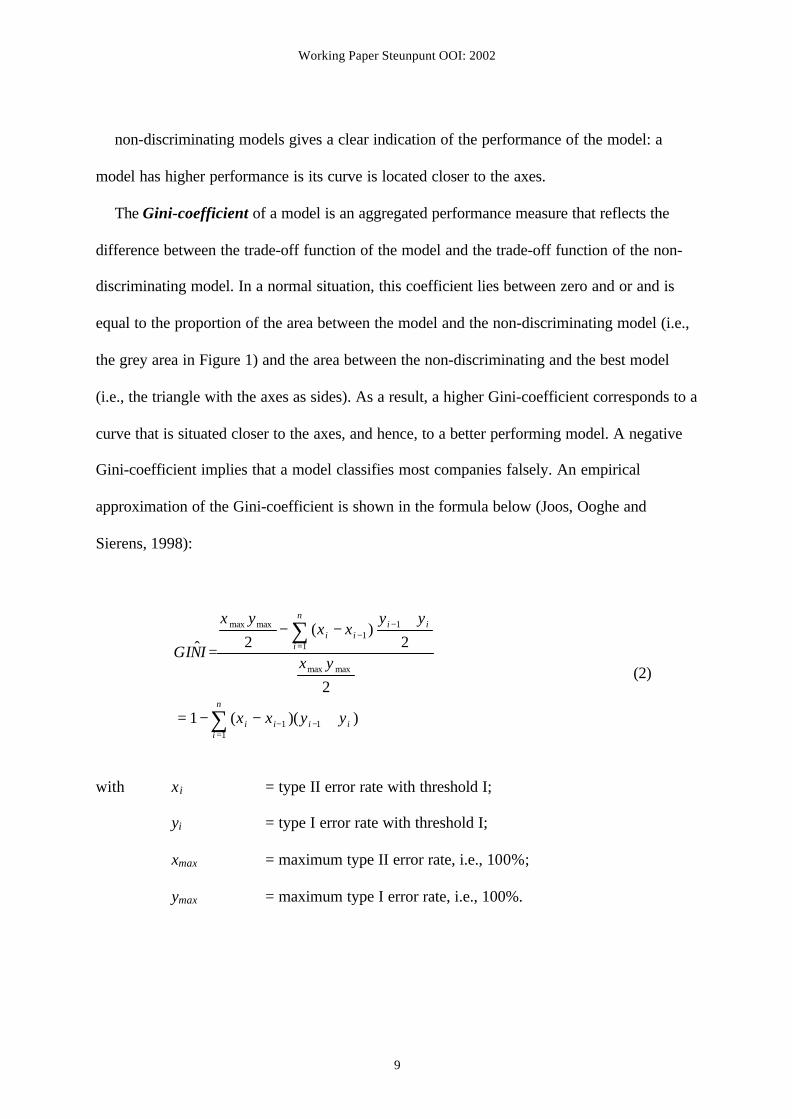
The Gini-coefficient of a model is an aggregated performance measure that reflects the
difference between the trade-off function of the model and the trade-off function of the non-
discriminating model. In a normal situation, this coefficient lies between zero and or and is
equal to the proportion of the area between the model and the non-discriminating model (i.e.,
the grey area in Figure 1) and the area between the non-discriminating and the best model
(i.e., the triangle with the axes as sides). As a result, a higher Gini-coefficient corresponds to a
curve that is situated closer to the axes, and hence, to a better performing model. A negative
Gini-coefficient implies that a model classifies most companies falsely. An empirical
approximation of the Gini-coefficient is shown in the formula below (Joos, Ooghe and
Sierens, 1998):
∑
∑
=−−
=
−−
+−−=
+−−
=
n
iiiii
n
i
iiii
yyxx
yx
yyxx
yx
INGI
111
maxmax
1
11
maxmax
))((1
2
2)(
2ˆ
(2)
with xi = type II error rate with threshold I;
yi = type I error rate with threshold I;
xmax = maximum type II error rate, i.e., 100%;
ymax = maximum type I error rate, i.e., 100%.

Working Paper Steunpunt OOI: 2002
10
2. FAILURE PREDICTION MODELS
Because the aim of the study is to compare the validity of a range of failure prediction
models from different countries, that have been published over the years, we have to select a
number of models. In the selection process, several criteria are taken into account.
Firstly, as already mentioned, this study only focuses on models estimated with linear
discriminant analysis and logistic regression.
Secondly, we restrict ourselves to the analysis of models that are ‘frequently referred to’ in
research papers. For example, on the basis of this criterion, the Altman (1968) model and the
Zavgren (1983) model are included in this study.
Thirdly, the availability of variable and coefficient information is an important criterion.
As many recent models are licensed to commercial companies, they are not fully described in
academic publications and therefore could not be included in this study. One example of a
model that is excluded because of the unavailability of coefficients is the Taffler (1984)
model.
Furthermore, the ease of use of the models with respect to the calculation of the variables
is taken into consideration. Models that include non-financial data, such as gross national
product, are left out of this study. For example, the Ohlson model (1980), which includes the
GNP price index, is excluded from the analysis.
In addition, this study only incorporates ‘developed country models’ (Altman and
Narayanan, 1997). ‘Developing country models’ fall outside the study, as we expect these
models to show extremely large error rates when validated on Belgian annual accounts. In
developing countries, free market economies do not occur and it is difficult to detect company
failure because of the degree of government protection.

Working Paper Steunpunt OOI: 2002
11
Finally, we opt for general models and hence exclude models investigating the probability
of failure of, for example, new, high-tech or small firms. One example concerns the exclusion
of the Laitinen model (1992), which was designed to predict failures of newly founded firms.
At the end of the selection procedure, eight models remain: Altman (1968), USA;
Bilderbeek (1979), The Netherlands; Ooghe−Verbaere (1982), Belgium; Zavgren, (1985)
USA; Gloubos−Grammatikos (discriminant analysis and logistic regression) (1988), Greece;
Keasey−McGuinness (1990), United Kingdom; and Ooghe−Joos−De Vos (1991), Belgium. In
Appendix 1, Table 1 summarizes the characteristics of each of these eight models, and in
Tables 2 to 8 the variables of the models are shown. In these tables, each different variable is
attributed a unique name (X1, X2,…, X40). Detailed analysis of the variables reveals that the
same variables are frequently used in several models.
The signs of the original coefficients must be defined according to the general settings of
this study. As already mentioned, in this paper a high (logit or discriminant) score indicates a
healthy financial situation. The signs of the original coefficients of all models in Tables 2 to 8
in Appendix 1 are defined accordingly. Therefore, for some models, the signs of the original
coefficients are opposite to those reported in the original papers of the authors.
However, comparing the performances of the different models in their current form (i.e.,
with their original variables and original coefficients) will cause some difficulties. We should
bear in mind that models perform badly out-of-sample when there is a large difference
between the estimation sample and the validation sample, especially if the differences are the
result of differences in the definitions of the dependent variables, exogenous factors (such as
macroeconomic conditions and institutional and legal factors unique to the country of origin)
and the sample period. It is clear that the calculation of the original coefficients of the various
models was influenced by the correlations between the variables that are included in the

Working Paper Steunpunt OOI: 2002
12
original estimation samples and the variables that are not included in these samples, such as
macroeconomic conditions, institutional factors and sample period. Consequently, if we
validate the models with their original coefficients on the Belgian data, we will be unable to
determine whether bad performance of the models is the consequence of an inappropriate
choice of the variables or of the use of coefficients that fail to capture the true relationship
between the variables and failures of Belgian companies.
The re-estimation of the coefficients of all models over the Belgian data using the original
variables, will allow the models to take into account some factors specific to the Belgian
validation dataset. As a result, we will be able to compare model performances more
precisely, and to indicate whether the performance results can be explained solely by the
choice of variables. In this view, it is clear that, besides the validation of the models with their
original coefficients, we must also validate the models with their re-estimated coefficients.
3. POPULATION AND SAMPLES
Before describing the population and the sampling method for re-estimation and validation,
it seems appropriate to give some important definitions that are frequently used in this study.
3.1. Definitions of Failing and Non-Failing Firms
A ‘failing’ firm is a firm in the situation of bankruptcy, or with a request for a judicial
composition, or with an official approval of a judicial composition.
On the other hand, firms that are characterized by the following juridical situations are
included in the group of ‘non-failing’ firms:
- Termination of activity;
- Early dissolution−liquidation;
- Liquidation followed by a merger with another company;
Working Paper Steunpunt OOI: 2002
13
- Liquidation followed by absorption by another company;
- Closing of a liquidation;
- Without any particular legal status.
In other words, not only ‘normal’ firms without any particular legal status, but also firms
with associated doubts about the economic reasons for their juridical situation are included in
the non-failing population. As it is our aim to validate failure prediction models, it is
necessary to measure the performance of the models in a realistic situation, and hence
consider these doubt-causing firms as non-failing ones. However, when re-estimating the
coefficients of the failure prediction models, we want to reduce the influence of these doubt-
causing firms. Therefore, in the ‘re-estimation sample’, which is discussed in Section 4.3,
only firms without any particular legal status are included in and all other firms are ruled out
of the group of non-failing firms.
3.2. Population and Samples of Failing and Non-Failing Companies
This study is based on Belgian accounting data from the period 1994−1999. It concerns
published annual accounts of non-financial companies subject to the legislation on the annual
accounts of companies. The data were obtained from the CD-ROMs of Bureau Van Dijk and
information supplier Graydon NV.
The total population of companies consists of all firms having published at least one
annual account in the period 1994−1999. Companies that are classified into the following
activity classes, are excluded because of their special situations:
- Financial intermediation, insurance and pension funding;
- Management activities of holding companies and co-ordination centres;

Working Paper Steunpunt OOI: 2002
14
- Public administration, defence, services to the community as a whole, and compulsory social
security;
- Education;
- Health and social work;
- Activities of membership organizations;
- Private households with employed persons;
- Extra-territorial organizations and bodies.
The total population comprises 268.465 companies, identified by their V.A.T. numbers.
From this total population, two samples are taken: a sample of failing companies and a sample
of non-failing firms.
It should be noted that, in Belgium, companies are required to deposit their annual
accounts in a prescribed form, dependent on their size. A distinction is to be made between
‘large’ companies that must prepare their annual accounts in a complete form, and ‘small’
companies that are allowed to prepare their annual accounts in an abbreviated form. The
group of larger companies consists of companies with more than 100 employees, plus
companies that meet at least two of the following three criteria:
- Number of employees (yearly average): more than 50;
- Turnover (V.A.T. excluded) (yearly average): more than 200 million Belgian francs;
- Total assets: more than 100 million Belgian francs.
In Belgium, a major percentage of the companies have annual accounts in an abbreviated
form: in 1999, only 6,2% of the total population of companies deposited a complete-form
annual account.
The sample of failing companies consists of all firms that failed in 1997 or 1998. Only
firms that failed in 1997 having annual accounts in 1994 or later, and firms that failed in 1998

Working Paper Steunpunt OOI: 2002
15
having annual accounts in 1995 or later, are included. The failing sample comprises 6500
companies.
On the other hand, the sample of non-failing companies includes all firms that are non-
failing on January 1, 1999, and that have annual accounts in 1994 or later. The non-failing
sample involves 249.334 companies.
Table 1 illustrates the number of failing and non-failing companies that are used in this
study. It also reports the percentage of the non-failing sample that is made up of companies
characterized by the judicial situations mentioned in the list in Section 4.1.
Insert Table 1 about here
3.3. Samples of Failing and Non-Failing Annual Accounts
The sampling procedure for the samples of failing annual accounts is rather simple.
Because the aim of the study is to re-estimate and to validate the models one, two and three
years prior to failure (i.e., 1 ypf, 2 ypf and 3 ypf), we select the annual accounts one, two and
three years prior to failure (if available and if not concerning an extended fiscal year) for each
company in the failing sample. However, not all companies deposit their annual accounts on
December 31. Consequently, the annual accounts 1, 2 and 3 ypf are defined as follows:
Account one year prior to failure: account with the closing date falling within the period
[date of failure, date of failure − 365 days]
Account two years prior to failure: account with the closing date falling within the period
[date of failure − 365 days, date of failure − (2 * 365 days)]
Account three years prior to failure: accounts with the closing date falling within the period
[date of failure − (2 * 365 days), date of failure − (3 * 365 days)]
Working Paper Steunpunt OOI: 2002
16
To select the samples of non-failing annual accounts, the group of non-failing companies
is randomly divided into four equal groups: groups A, B, C and D. For each group of
companies, the annual accounts of one specific year in the period 1994−1997, if available and
if not concerning an extended fiscal year, are taken. The following non-failing annual
accounts are selected:
Non-failing firms in group A: annual accounts of 1994
Non-failing firms in group B: annual accounts of 1995
Non-failing firms in group C: annual accounts of 1996
Non-failing firms in group D: annual accounts of 1997
In this study, we link the failing annual accounts one, two and three years prior to failure to
the non-failing annual accounts, bearing in mind that the annual accounts of the two different
samples should refer to the same time frame. Accordingly, for each year prior to failure, the
annual accounts of the two relevant years are taken together. This procedure is explained in
Table 2. The resulting numbers of annual accounts in the samples of failing and non-failing
annual accounts are reported in Table 3.
Insert Table 2 about here
Insert Table 3 about here
Because we want to re-estimate the coefficients of the eight models on the Belgian data
before validation, we require validation and re-estimation samples of failing and non-failing
annual accounts. Consequently, the samples of failing and non-failing annual accounts are
randomly divided into separate re-estimation samples and validation samples. Within each

Working Paper Steunpunt OOI: 2002
17
sample of failing and non-failing annual accounts, 50% of the accounts are classified as a re-
estimation sample, and 50% are included in a validation sample.
As already mentioned, in the re-estimation samples, the annual accounts of ‘doubt-
causing’ firms, must be excluded from the group of non-failing annual accounts. Only
companies without any particular legal status should be considered as non-failing.
Furthermore, we are forced to reduce the large number of non-failing annual accounts in the
re-estimation samples because of the practical limitations of the statistical programme used.
In this respect, about 20% of the non-failing annual accounts are selected randomly. In
contrast, the number of failing annual accounts is not reduced. Finally, we eliminate all
annual accounts that have not been deposited at the National Bank of Belgium and therefore
are not available on the CD-ROMs of Bureau Van Dijk. This significantly reduces the
original number of failing annual accounts in the sample, at 1 ypf in particular, as many
failing companies cease to pay attention to financial reporting when they are close to failure.
Also, the annual accounts of non-failing companies founded after 1 January, 1998 are
excluded, because these companies do not have annual accounts in the period 1994-1997.
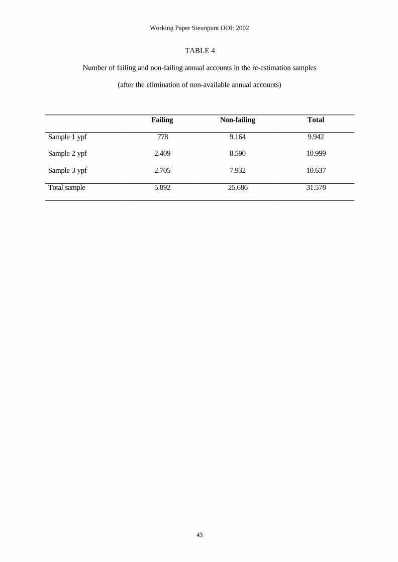
Table 4 presents the number of failing and non-failing annual accounts in the 1 ypf, 2 ypf and
3 ypf estimation samples after the elimination of non-available annual accounts.
Insert Table 4 about here
It is clear that some models have different variables and coefficients depending on the
period within which they aim to predict failure. Ooghe−Verbaere, Keasey−McGuinness and
Ooghe−Joos−De Vos do not use the same variables for failure predictions one, two and three
years prior to failure. These models are re-estimated on the basis of the corresponding re-
estimation samples, being the samples 1, 2 and 3 ypf. In addition, the Zavgren model, which
Working Paper Steunpunt OOI: 2002
18
uses the same variables but different coefficients for failure prediction one, two and three
years prior to failure, is re-estimated on the basis of these three samples.
On the other hand, the models that make no distinction between failure prediction one, two
and three years prior to failure − being Altman, Bilderbeek, and Gloubos−Grammatikos
discriminant and logit − use the same variables and coefficients independent of the year prior
to failure. They only have ‘general’ coefficients and hence are re-estimated on a ‘general’
sample (i.e., ‘total sample’ in Table 4), which is composed of all annual accounts in the 1 ypf,
2 ypf and 3 ypf samples.
The validation samples of failing and non-failing annual accounts are taken in much the
same way as the re-estimation samples. As with the re-estimation samples, the number of
non-failing annual accounts is much too large to be able to use the statistical programme.
Again, this large number of non-failing annual accounts must be reduced: about 20% of the
non-failing annual accounts were selected randomly. In addition, all annual accounts that have
not been deposited are excluded from the validation samples. Again, this reduces the original
number of failing annual accounts in the sample 1 ypf significantly. Table 5 reports the
number of failing and non-failing annual accounts in the 1 ypf, 2 ypf and 3 ypf validation
samples after the elimination of non-available annual accounts.
Insert Table 5 about here
On the basis of each annual account in the re-estimation samples, we calculate a range of
variables or ratios (i.e., the variables X1 to X40 referred to in Tables 2 to 8 in Appendix 1) to
re-estimate the coefficients of the models. On the other hand, on the basis of each annual
account in the validation samples, we compute a (logit or discriminant) score for each model
Working Paper Steunpunt OOI: 2002
19
to determine the model performance. Here, it is important to mention the influence of invalid
observations, both in the re-estimation and in the validation process.
Firstly, a detailed examination of the data concerning the variables reveals a frequent
occurrence of invalid variables, caused by zero values in the denominators of the variables.
This is particularly the case if the denominator of a variable contains sales or inventories.
According to Belgian accounting law, approximately half of the small companies, publishing
their results in an abbreviated form, only state their ‘gross margin’ as they are not obliged to
publish sales and operating costs. Furthermore, some types of companies (for example service
firms) simply do not have inventories.
As a result, when re-estimating each of the models, a certain percentage of the annual
accounts in the re-estimation samples show invalid observations for some variables, and
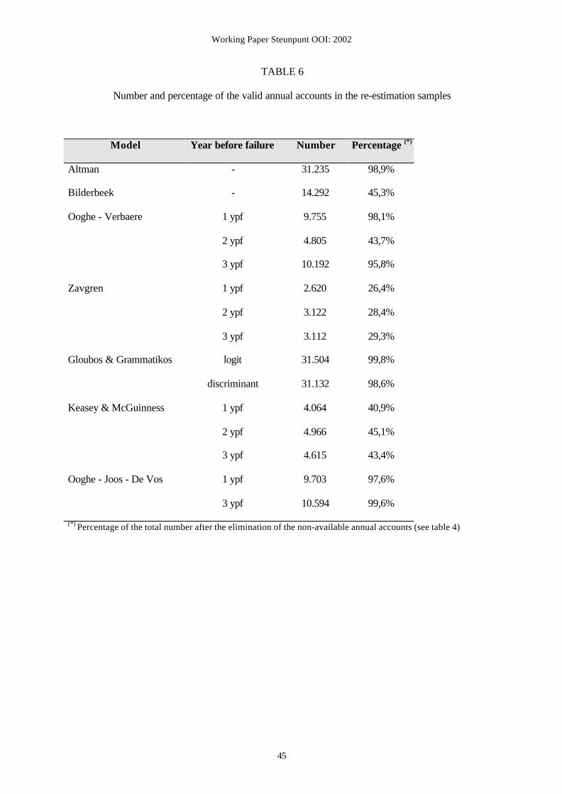
hence cannot be used. Table 6 gives an overview of the percentage of annual accounts that
could be used for the re-estimation of each of the models. For example, when re-estimating
the Zavgren model, less than 30% of the annual accounts can be used, because the model uses
ratios containing sales and inventories in their denominator. Furthermore, when re-estimating
other models with ratios containing ‘sales’ in their denominator (Bilderbeek, Ooghe−Verbaere
2 ypf, and Keasey−McGuinness), less than 50% of the annual accounts in the re-estimation
samples can be used.
Insert Table 6 about here
In this respect, we should bear in mind that, as the models use different variables, they are
not re-estimated on the basis of the same samples of annual accounts. However, this causes no
problems for the re-estimation process, because it is our aim to calculate the re-estimated

Working Paper Steunpunt OOI: 2002
20
coefficients for each of the models as precisely as possible. Consequently, we want to include
as many annual accounts as possible for each individual model.
Secondly, detailed analysis of the data on the logit and discriminant scores also reveals the
presence of invalid scores, caused by invalid variables. However, when validating the models
it is important that the performance results are based on the same samples of annual accounts,
as it is our aim to compare the results of the different models on an equal basis. Consequently,
all annual accounts that show an invalid score for at least one model are excluded from the
validation samples. Only the annual accounts that have valid scores for each model are
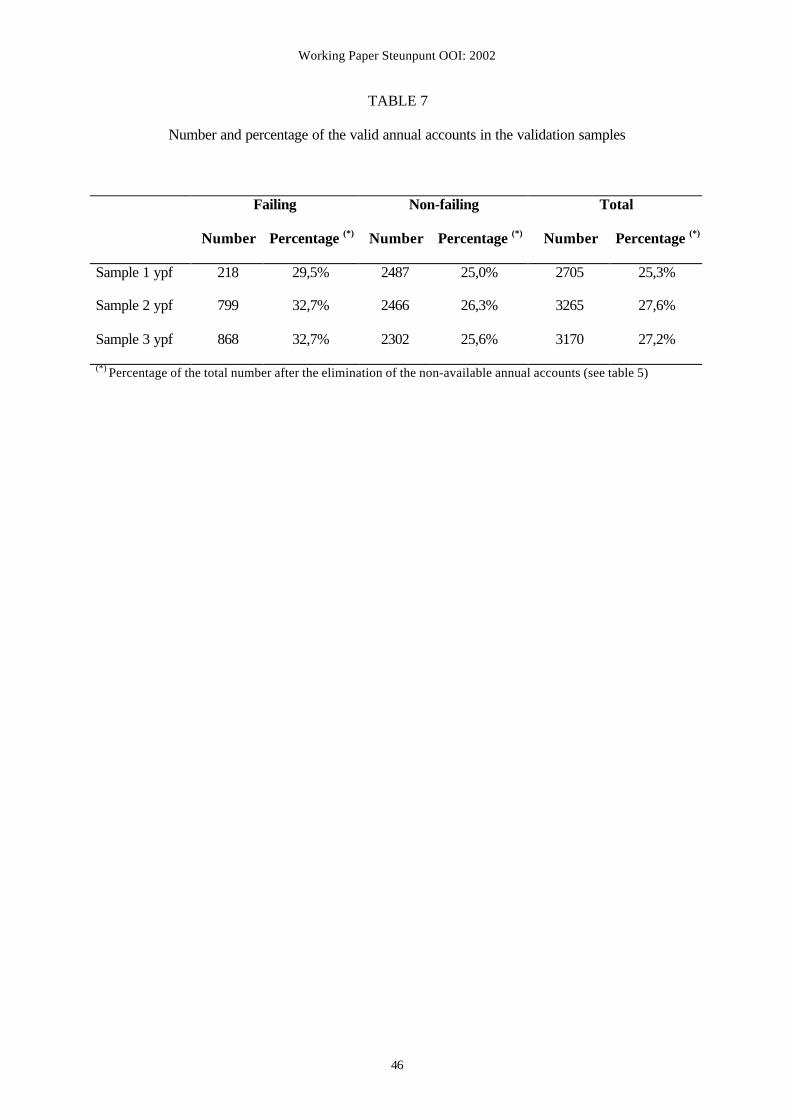
selected. Table 7 reports the number of annual accounts that are finally included in the
validation sample. This is the total number of annual accounts that are used to validate the
models.
Insert Table 7 about here
4. RESULTS AND INTERPRETATION
This section discusses the validation results of the different failure prediction models on
the dataset of Belgian companies. Section 5.1 gives some preliminary remarks on the signs of
the coefficients of the variables. As an illustration, Table 9 in Appendix 1 shows the
validation results obtained by the authors of the models in their original studies. The
performance results of the different models using the original coefficients are reported in
Section 5.2. We discuss the type I, type II, and unweighted error rates corresponding to the
optimal cut-off points of the models, and we calculate Gini-coefficients. We also give a
graphical illustration of the results by means of trade-off functions. In Section 5.3, we analyse
the performance results of the models with the re-estimated coefficients. Section 5.4 gives an
overview of all validation results and discusses the change in performance results when using

Working Paper Steunpunt OOI: 2002
21
the re-estimated coefficients instead of the original ones. Finally, in Section 5.5 we put
forward some possible explanations for the dispersed performances.
4.1. Preliminary Remarks on the Signs of the Variables
The failure prediction models are re-estimated using the re-estimation samples and are
attributed new coefficients and new optimal cut-off points. These new coefficients and cut-off
points are reported in Tables 2 to 8 in Appendix 1. A detailed analysis of the signs of the
original and the new coefficients reveals that some of these signs do not correspond to
expectations.
First, the signs of the coefficients of several variables in the original models do not match
expectations:
• Appendix 1, Table 3: Bilderbeek (1979): variables X6 and X5;
• Appendix 1, Table 5: Zavgren (1985): variables X19, X21, X6 and X22;
• Appendix 1, Table 6: Gloubos and Grammatikos (1988): variables X23 and X11;
• Appendix 1, Table 7: Keasey and Mc Guinness (1990): variables X4 and X18.
On the other hand, some of the new, re-estimated coefficients also have unexpected signs:
• Appendix 1, Table 2: Altman (1968): variables X1 and X5;
• Appendix 1, Table 3: Bilderbeek (1979): variables X6, X7, X8 and X2;
• Appendix 1, Table 4: Ooghe and Verbaere (1982): variables X9 and X14 (3 ypf);
• Appendix 1, Table 5: Zavgren (1985): variables X19 (2 ypf and 3 ypf), X21 (1 ypf), X
6 (1 ypf and 2 ypf) , X22 and X5;
• Appendix 1, table 7: Keasey and McGuinness (1990): variables X26 (1 ypf), X18 and
X5;
• Appendix 1, table 8: Ooghe, Joos and de Vos (1991): variables X32 and X40;

Working Paper Steunpunt OOI: 2002
22
The (linear) multivariate contexts of the models are the only possible explanation for these
unexpected signs: the (positive or negative) influence of some variables are counterbalanced
by the (negative or positive) influence of other variables.
4.2. Performance Results of the Failure Prediction Models with the Original Coefficients
The validation results of the models with their original coefficients are shown in Table 8.
The best-performing models are indicated in bold letters, while the worst-performing models
are printed in italic. Firstly, Table 8 reports the type I, type II and unweighted error rates
corresponding to the new optimal cut-off points of the models. The optimal cut-off point is
equal to the score for which the unweighted average of the type I and type II error rates
reaches a minimum (see section 2.2.1). Besides the unweighted error rate, the Gini-coefficient
can also be used to evaluate the ‘fit’ of the models. Contrary to the discussion of the type I
and type II errors separately, this measure gives a global judgement of performance: the Gini-
coefficient is independent of changing cut-off points. Finally, Table 8 shows the rankings of
the models, both on the basis of the UER and the Gini-coefficient. These rankings clearly
indicate which models perform best or worst, 1 ypf, 2 ypf and 3 ypf.
Insert Table 8 about here
Analysis of the unweighted error rates, the Gini-coefficients and the rankings of the models
one year prior to failure reveals that the Belgian Ooghe−Joos−De Vos model performs best,
followed closely by the models of Ooghe−Verbaere and Bilderbeek. On the contrary,
Zavgren, Gloubos−Grammatikos discriminant and Keasey−McGuinness seem to be less
successful in predicting failure.
The results of the models two years prior to failure are similar to the results of the short-
term models: Bilderbeek and Ooghe−Verbaere are indicated as the best-performing models.

Working Paper Steunpunt OOI: 2002
23
In addition, the Gloubos−Grammatikos logit model seems to have a very high Gini-
coefficient. On the other hand, Zavgren clearly shows the highest UER and the lowest Gini-
coefficient.
The performance results of the models three years prior to failure indicate the
Ooghe−Joos−De Vos model as the model with the best failure prediction results, and, as in the
short-term case, Ooghe−Verbaere and Bilderbeek follow closely. Again, the Zavgren model
seems to be the worst failure predictor.
In Figures 1 to 3 in Appendix 2, we plot the trade-off functions of the models 1, 2 and 3
ypf using the original coefficients. Figure 1, which reports the results of the short-term (1 ypf)
models, indicates Ooghe−Joos−De Vos, Ooghe−Verbaere and Bilderbeek as the best-
performing models. Figure 2 indicates Bilderbeek, Ooghe−Verbaere and also
Gloubos−Grammatikos logit as the models that have the most predictive abilities two years
prior to failure. Figure 3 reveals that Ooghe−Joos−De Vos, Bilderbeek, and Ooghe−Verbaere
perform best three years prior to failure.
It is noteworthy that if the term of the failure prediction is longer, the average unweighted
error rate of the models increases, and the average Gini-coefficient decreases: the average
UER of the short-term models is significantly lower than the average UER of the 2 ypf and 3
ypf models. This finding is not surprising as it is generally believed that it is easier to predict
failure, and hence discriminate between failing and non-failing companies in the short term.
One of the reasons for this finding is that specific features of failing companies are less
pronounced three years before failure than they are one year before failure.

Working Paper Steunpunt OOI: 2002
24
Finally, it should be noted that, when using the original coefficients, the performance
differences between the models are quite small. In addition, it is clear that the performance
differences depend on the term of failure prediction. A comparison of the distributions of the
trade-off functions (see Figures 1 to 3 in Appendix 2) reveals that the performance differences
between the best and the worst short-term (1 ypf) models are significantly larger than the
differences for the 2 ypf and the 3 ypf models. Consequently, if the term of failure prediction
is longer, it seems to be more difficult to make a distinction between good and bad
performing models.
4.3. Performance Results of the Failure Prediction Models With the Re-estimated
Coefficients
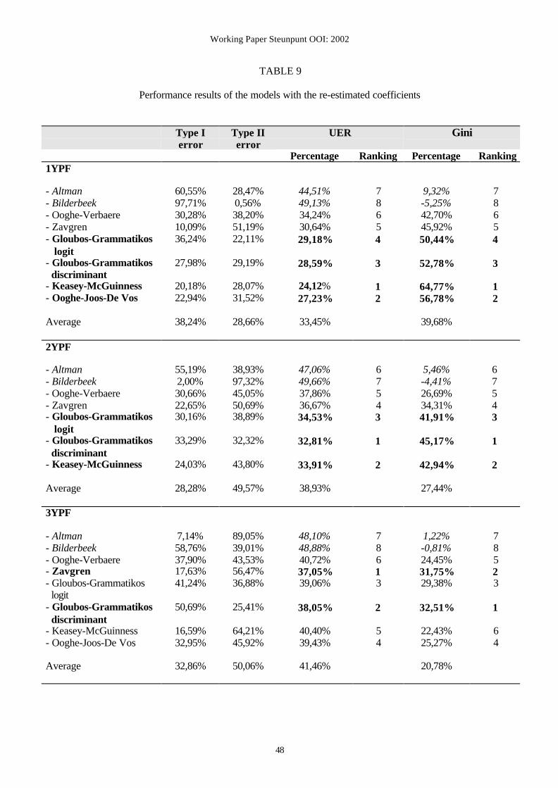
Table 9 reports the validation results (the error rates, Gini-coefficient and rankings) of the
models with their new, re-estimated coefficients. As in Table 8, the best-performing models
are highlighted in bold letters, while the worst-performing models are indicated in italic.
Compared to the results presented above, the results in table 9 show a totally different view.
Table 9 about here
The performance results of the models one year prior to failure indicate
Keasey−McGuinness as the best performing model. In addition, Ooghe−Joos−De Vos, and
both Gloubos−Grammatikos models (discriminant and logit) reveal very small unweighted
error rates. On the contrary, the Bilderbeek and Altman models perform worst. The
Bilderbeek model even has a negative Gini-coefficient, which means that the models
classifies most companies falsely.
With respect to the models two years prior to failure, Gloubos−Grammatikos discriminant
performs best, followed closely by Keasey−McGuinness and Gloubos−Grammatikos logit.

Working Paper Steunpunt OOI: 2002
25
Furthermore, as in the short-term case, Bilderbeek and Altman reveal the highest UER and the
lowest Gini-coefficient and hence are the worst performing models.
Examination of the results of the models three years prior to failure reveals that the
Zavgren and the Gloubos−Grammatikos discriminant models are the ones that perform best.
Again, Bilderbeek and Altman clearly are the worst failure predictors.
The trade-off functions of the models 1, 2 and 3 ypf using the re-estimated coefficients are
shown in Figures 4 to 6 in Appendix 2. From Figure 4 concerning the short-term (1 ypf)
models, it is apparent that four models have very high predictive abilities:
Keasey−McGuinness, Ooghe−Joos−De Vos and Gloubos−Grammatikos discriminant and
logit. Figure 5 indicates Gloubos−Grammatikos discriminant and logit, and
Keasey−McGuinness as the best-performing 2 ypf models. Observation of Figure 6 suggests
that Zavgren and Gloubos−Grammatikos discriminant show the best results with respect to
long-term failure prediction. In addition, the trade-off function of the Gloubos−Grammatikos
logit model seems to be very close to the axes.
When using the re-estimated coefficients, analysis of the average unweighted error rates
and Gini-coefficients leads to the same conclusions as with the original coefficients (see
Section 5.2). If we want to predict failure over a longer term, the average UER increases, and
the average Gini-coefficient decreases. Again, the results confirm the general belief that it is
easier to predict failure in the short term.
The performance results of the models with re-estimated coefficients reveal larger
performance differences in comparison to the results with respect to the original coefficients.
For example, the short-term (1 ypf) models with re-estimated coefficients show a variation in

Working Paper Steunpunt OOI: 2002
26
the UER of no less than 25,01%. Also, when analysing the general distribution of the trade-
off functions in Figures 4 to 6 in Appendix 2, it is immediately apparent that the performance
differences depend on the term of failure prediction. The difference between the trade-off
functions of the best- and the worst-performing short-term (1 ypf) models is extremely large.
The performance differences for the 2 ypf models are significantly smaller and, finally, the
long-term (3 ypf) models reveal the smallest performance differences. Consequently, when
using the re-estimated coefficients, the results again suggest that it is more difficult to indicate
models with good and bad performance if the term of failure prediction is longer.
4.4. Change in Performance Results Before and After Re-estimation of the Coefficients
and Overall Performance Results
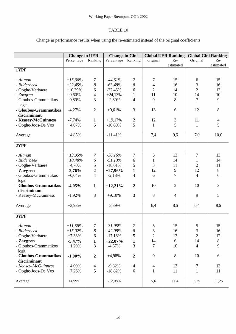
If we compare the performance results of the models with their original coefficients (Table
8) to the results of the models with their re-estimated coefficients (Table 9), we find some
important differences. Table 10 summarizes the results. For each model, Table 10 shows the
change in the UER and Gini-coefficient when using the re-estimated coefficients instead of
the original ones and it gives rankings according to these changes. Moreover, it shows the
global ranking (i.e., with the original and with the re-estimated coefficients) of the models 1
ypf, 2 ypf and 3 ypf, both on the basis of the unweighted error rates (UER-ranking) and on the
basis of the Gini-coefficients (Gini-ranking).
Insert Table 10 about here
Firstly, the rankings (both on the basis of the UER and the Gini-coefficients) of the models
with the original coefficients (Table 8, columns 5 and 7) differ significantly from the rankings
of the models with the re-estimated coefficients (Table 9, columns 5 and 7). For example, the
Bilderbeek model, which is one of the best-performing models 1, 2 and 3 ypf when using the

Working Paper Steunpunt OOI: 2002
27
original coefficients, loses an important part of its predictive abilities when its coefficients are
re-estimated. This causes the model to be indicated as the worst-performing model 1, 2 and 3
ypf in Table 9. On the contrary, one year prior to failure, the Gloubos−Grammatikos
discriminant and Keasey−McGuinness models perform very badly with the original
coefficients, whereas they are among the best-performing models when using the re-estimated
coefficients. In addition, with their original coefficients, Zavgren and Gloubos−Grammatikos
discriminant are the worst-performing 3 ypf models, whereas they seem to be the models with
the best predictive abilities 3 ypf after re-estimation of their coefficients.
A detailed examination of the changes in the unweighted error rates and the changes in
the Gini-coefficients for each model when using the re-estimated coefficients instead of the
original ones (table 10 columns 2 to 5) reveals that, after re-estimation, some models improve
their failure prediction abilities, while others show worse performance results. Generally,
when re-estimating the coefficients, the models that perform best with the original
coefficients (small UER and a high Gini-coefficient in Table 8) deteriorate (increase of the
UER and decrease of the Gini-coefficient in Table 10). On the other hand, models that
perform very badly with the original coefficients improve (decrease of the UER and increase
of the Gini-coefficient in Table 10). This is an interesting finding, because, in contrast to
expectations, re-estimation does not improve the performance results for all models.
Table 10 reveals that after re-estimation the average failure prediction power of the
models (1 ypf, 2 ypf and 3 ypf) deteriorates: the average UER increases, the average Gini-
coefficient decreases, and the average UER-rankings and Gini-rankings with respect to the re-
estimated coefficients are less favourable in comparison with the average rankings for the
original coefficients.

Working Paper Steunpunt OOI: 2002
28
Its is remarkable that, on an overall comparison (with the original coefficients and with the
re-estimates ones), the best-performing models are the models with the original, non re-
estimated coefficients:
- 1 ypf: Ooghe−Joos−De Vos and Ooghe−Verbaere;
- 2 ypf: Bilderbeek;
- 3 ypf: Ooghe−Joos−De Vos and Ooghe−Verbaere.
Moreover, it is important to mention that the globally best-performing 1 ypf and 3 ypf
models (Ooghe−Joos−De Vos and Ooghe−Verbaere) have a Belgian origin. The model that
performs best 2 ypf (Bilderbeek) is a Dutch model.
4.5. Possible Explanations for the Performance Results
There is no clear general answer whether failure prediction models are transferable from
one country or period to another one. Several explanatory factors for individual model
performance can be proposed:
1. the age of the model, measured by the period of deposit of the annual accounts included in
the estimation sample of the model;
2. the country of origin of the model, being the nationality of the companies from which the
annual accounts are included in the original estimation sample of the model;
3. the definition of failure that was applied to determine the estimation sample of failing
companies;
4. the types of companies that had their annual accounts included in the estimation sample of
the model;
5. the technique on which the estimation of the model is based;
6. the number of variables included in the model;

Working Paper Steunpunt OOI: 2002
29
7. the complexity of the variables included in the model;
8. the types of variables included in the model.
As discussed earlier, if we compare the performance results of the different models using
their original coefficients, we are unable to determine whether model performance is a
consequence of the variables that are included in the models (i.e., Factors 7 and 8), or of the
modelling technique (Factor 5). A bad performance result can also be caused by model
coefficients that fail to capture the true relationship between the independent variables and the
failures of Belgian companies. If there are large differences between the original estimation
sample of a model and the validation sample with respect to the time frame and the nationality
of the annual accounts, the definition of failure and the types of companies (i.e., Factors 1 to
4), the performance results of the model will be low, even if the model includes ‘the right’
variables and is based on ‘the right’ modelling technique.
By applying the re-estimated coefficients when validating the models, we take into
account some factors specific to the Belgian validation dataset. If we re-estimate all models
on the same re-estimation sample of Belgian companies, the following possible explanatory
factors can be eliminated: the age of the model, the country of origin, the definition of failure
and the type of companies. The remaining explanatory factors that should be considered are:
the estimation technique, the number of variables, the complexity of the variables, and the
type of variables.
Taking a closer look at the characteristics of the worst performing models after re-estimation
(Altman and Bilderbeek) and comparing these with the characteristics of models that show
better results (for example, Ooghe−Joos−De Vos, Gloubos−Grammatikos discriminant,
Working Paper Steunpunt OOI: 2002
30
Zavgren and Keasey−McGuinness), it is possible to indicate which of these factors are the
most important ones.
First, it is clear that the estimation technique does not have an influence on model
performance. Altman and Bilderbeek are estimated using linear discriminant analysis, but
some of the better-performing models are also based on this technique. Secondly, the
complexity of the variables does not seem to be an explanatory factor for model performance.
Altman and Bilderbeek include simple variables, but the better-performing models (for
example Keasey−McGuinness) also consist of rather simple variables. Furthermore, the
number of variables does not seem to have an important impact on the model performance.
For example, not only the worst performing Altman and Bilderbeek models, but also the
good-performing Gloubos−Grammatikos logit and discriminant models use the same
variables 1, 2 and 3 ypf. In addition, the Gloubos−Grammatikos logit model consists of only
three variables, while Altman and Bilderbeek have five variables.
On the other hand, the types of the variables (i.e., Factor 8) seem to be an explanatory
factor. On the basis of Tables 2 to 8 in Appendix 1, it is clear that the poorly performing
Altman and Bilderbeek models are primarily based on variables concerning profitability and
added value, whereas the better- performing models like Ooghe−Joos−De Vos, Zavgren and
Gloubos−Grammatikos also concentrate on solvency and liquidity. At least half of the
variables in these models concern liquidity or solvency.
Consequently, this study makes a strong case for including all aspects of financial health in
a failure prediction model. Solvency and liquidity seem to be as important as profitability and
added value!
Working Paper Steunpunt OOI: 2002
31
5. SUMMARY AND CONCLUSIONS
By examining the validity of a range of international failure prediction models on a dataset
of Belgian companies and by identifying these models that have the best and the worst failure
prediction ability, the aim of this study is to answer the question whether failure prediction
models from different countries can easily be transferred to other countries.
We validated eight international failure prediction models on one dataset of Belgian
company accounts. All models were based on one of the two basic modelling techniques in
failure prediction research: linear discriminant analysis and logistic regression.
The predictive abilities of the models were assessed on the basis of several performance
indicators. Firstly, we discussed type I, type II and unweighted error rates (UER)
corresponding to the optimal cut-off points. Secondly, we compared the models in a more
global way with Gini-coefficients and finally, the trade-off functions provided a graphical
presentation of the research results. These performance indicators were calculated both
corresponding to the original coefficients and to the re-estimated ones.
The study started by re-estimating the coefficients of all failure prediction models over the
Belgian dataset. In this way, we excluded the influence of some factors specific to the original
estimation sample, which allowed a more precise comparison of the performance results. In
addition, by using the re-estimated coefficients, it was possible to determine whether
performances were the result of the choice of variables and/or of the applied modelling
technique.
When using the original coefficients, the ranking order of the models differed significantly
from the ranking order when using the re-estimated coefficients. Contrary to expectations,
models that showed poor performance results with their original coefficients revealed an

Working Paper Steunpunt OOI: 2002
32
improvement when using the re-estimated coefficients, while models with good performance
revealed a decrease in performance when using the coefficients after re-estimation. On
average, the failure prediction power of the models deteriorated after re-estimation of the
coefficients. Overall, with and without re-estimated coefficients, the best-performing models
were those with the original, non re-estimated coefficients.
It is important to mention that the globally best-performing 1 ypf and 3 ypf models are the
Belgian Ooghe−Joos−De Vos and Ooghe−Verbaere models.
This study confirms the general belief that it is easier to predict failure in the short term:
the average error rate of the short-term models both with the original coefficients and with the
re-estimated ones seemed to be significantly lower than the average error rate of the long-term
models. Also, the performance differences seem to depend on the term of failure prediction: if
the term is longer, it seems to be more difficult to make a distinction between models that
perform well or poorly.
In general, it is not clear whether failure prediction models can be transferred to other
countries and/or periods. Several possible explanatory factors for model performance were
proposed. However, by re-estimating the coefficients of all models on the same sample of
Belgian annual accounts, the following factors could be eliminated: the age of the model, the
country of origin, the definition of failure, and the type of companies. Taking a closer look at
the other characteristics of the models, neither the estimation technique, the complexity of the
variables, nor the number of variables did seem to have a major influence on the model
performance. On the other hand, the types of variables used, turned out to be an important
explanatory factor. Models that are primarily based on variables concerning profitability and
added value, revealed higher error rates than models that also concentrate on solvency and

Working Paper Steunpunt OOI: 2002
33
liquidity. Consequently, this study makes a strong case for including all different aspects of
the financial situation in a failure prediction model.
In this paper, we validated eight failure prediction models from five different countries on
a dataset of Belgian company accounts (i.e., cells A and B in Table 11). Consequently, we
invite other researchers to include more failure prediction models from other countries than
Belgium in a more extensive validation study (i.e., extend cell B in Table 11) and to validate
these models also on company accounts of countries other than Belgium (i.e., analyse cells C
and D in Table 11) in order to find out whether the same results will be found.
Insert Table 11 about here
Working Paper Steunpunt OOI: 2002
34
REFERENCES
Altman, E.I.. 1968. Financial ratios, discriminant analysis and the prediction of corporate
bankruptcy. The Journal of Finance, vol. 23 no. 4: 589--609.
Altman, E.I.. 1993. Corporate Financial Distress and Bankruptcy, Second Edition. John Wiley
& Sons, New York.
Altman, E.I., Avery, R.B., Eisenbeis R.A., Sinkey J.F.. 1981. Application of Classification
Techniques in Business, Banking and Finance. JAI Press, Greenwich, Connecticut.
Altman, E.I., Marco, G., Varetto, F.. 1993. Corporate distress diagnosis: comparisons using
linear discriminant analysis and neural networks (the Italian experience). Journal of
Banking and Finance, vol. 18: 505--529.
Altman, E.I., Margaine, M., Schlosser, M., Vernimmen, P.. 1974. Statistical credit analysis in
the textile industry; A French experience. Journal of Financial and Quantitative
Analysis, March 1974.
Altman, E.I., Narayanan, P.. 1997. An international survey of business classification models.
Financial Markets, Institutions & Instruments, vol. 6 no. 2: 1--57.
Anonymous. 1997. Credit Risk Analysis, Applications in some European Central Banks and
Related Organisations. Working Paper presented at the ‘International Conference of the
European Committee of Central Balance Sheet Data Offices’, October 1997, Paris.
Beaver, W.. 1967. Financial Ratios as predictors of failure. Empirical Research in Accounting
Selected Studies, 1966 in Supplement to The Journal of Accounting Research, January
1967: 71--111.

Working Paper Steunpunt OOI: 2002
35
Bell, T., Ribar, G., Verchio, J.. 1990. Neural nets versus logistic regression: a comparison of
each model’s ability to predict commercial bank failures. Paper presented at the Cash
Flow Accounting Conference, Nice (France), 1--8.
Bilderbeek, J.. 1979. De continuïteitsfactor als beoordelingsinstrument van ondernemingen.
Accountancy en Bedrijfskunde Kwartaalschrift, vol. 4 no. 3: 58--61.
Curram, S., Mingers, J.. 1994. Neural Networks, Decision tree induction and discriminant
analysis: an empirical comparison. Operational Research Society, vol. 45 no. 4: 440--
450.
Fernandez, A.I.. 1988. A Spanish model for credit risk classification. Studies in Banking and
Finance, vol. 7: 115--25.
Gloubos, G., Grammatikos, T.. 1988. Success of bankruptcy prediction models in Greece.
Studies in Banking and Finance: International business failure prediction models, vol. 7:
37--46.
Hosmer, D.W., Lemeshow, S.. 1989. Applied Logistic Regression. John Wiley & Sons, New
York.
Jones, F.. 1987. Current techniques in bankruptcy prediction. Journal of Accounting
Literature, vol. 6: 131--164.
Joos, Ph., Ooghe, H., Sierens, N.. 1998. Methodologie bij het opstellen en beoordelen van
kredietclassificatiemodellen. Tijdschrift voor Economie en Management, vol. 43 no. 1:
3--48.
Kankaanpää, M., Laitinen, T.. 1999. Comparative analysis of failure prediction methods: the
Finnish case. The European Accounting Review, vol. 8 no. 1: 67--92.
Keasey, K., McGuinness, P.. 1990. The failure of UK industrial firms for the period 1976-
1984: Logistic analysis and entropy measures. Journal of Business Finance and
Accounting, vol. 17 no. 1: 119--135.

Working Paper Steunpunt OOI: 2002
36
Koh, H.C.. 1992. The sensitivity of optimal cut-off points to misclassification costs of type I
and type II errors in the going concern prediction context. Journal of Business Finance
and Accounting, vol. 19 no. 2: 187--197.
Lachenbruch, P.A.. 1975. Discriminant Analysis. Hafner Press, McMillan, London.
Laitinen, E.K.. 1992. Prediction of Failure of a Newly Founded Firm. Journal of Business
Venturing, vol. 7 no. 4: 323--40.
Maddala, G.S.. 1983. Limited-Dependent and Qualitative Variables in Econometrics.
Cambridge University Press, New York.
Maddala, G.S.. 1992. Introduction to Econometrics. Maxwell, MacMillan, New York.
Mossman, C. E., Bell, G. G., Turtle, H., Swartz, L. M.. 1998. An empirical comparison of
bankruptcy models. The Financial Review, vol. 33: 35--54.
Nobes, C., Parker, R.. 2000. Comparative International Accounting, 6th Edition. Prentice
Hall, New Jersey.
Nygard, F., Sandström, A.. 1989. Income inequality measures based on sample surveys.
Journal of Econometrics, vol. 4: 81--95.
Ohlson, J. A.. 1980. Financial ratios and the probabilistic prediction of bankruptcy. Journal of
Accounting Research, Spring 1980: 109--131.
Ooghe, H., Verbaere, E.. 1982. Determinanten van faling: verklaring en predictie.
Unpublished paper, Department of Corporate Finance, Accountancy and Management
Information, Ghent University, Belgium.
Ooghe, H., Joos, Ph., De Vos, D.. 1991. Failure prediction models. Working Paper,
Department of Corporate Finance, Ghent University, Belgium.
Ooghe, H., Joos, Ph., De Bourdeaudhuj, C.. 1995. Financial distress models in Belgium: the
results of a decade of empirical research. The International Journal of Accounting, vol.
30 no. 3: 245--274.

Working Paper Steunpunt OOI: 2002
37
Ooghe, H., Van Wymeersch, C.. 2001. Financiële analyse van de onderneming. Kluwer
Ced.Samsom, Diegem, Belgium.
Shannon, C.E.. 1948. A mathematical theory of communication. Bell System Technical
Journal, vol. 27, July and October 1948: 379--423 and 623--656.
Siegel, S., Castellan, N.J.. 1988. Nonparametric Statistics for the Behavioural Sciences.
McGraw-Hill, New York.
Steele, A.. 1995. Going concern qualifications and bankruptcy prediction. Working Paper
presented at Doctoral Workshop Leuven, March 1995, Leuven.
Swanson, E., Tybout, J.. 1988. Industrial bankruptcy determinants in Argentina. Studies in
Banking and Finance, vol. 7: 1--25.
Taffler, R.. 1984. Empirical models for the monitoring of UK corporations. Journal of
Banking and Finance, vol. 8: 199--227.
Taffler, R.J., Tisshaw, H.J. 1977. Going, going, gone - Four factors which predict.
Accountancy, March 1977: 50--54.
Theil, H.. 1971. Principles of Econometrics. North-Holland Publishing Company,
Amsterdam, The Netherlands.
Zavgren, C.. 1983. The prediction of corporate failure: the state of the art. Journal of
Accounting Literature, vol. 2: 1--33.
Zavgren, C.. 1985. Assessing the vulnerability to failure of American industrial firms: a
logistic analysis. Journal of Business Finance and Accounting, Spring 1985: 19--45.

Working Paper Steunpunt OOI: 2002
38
APPENDIX 1 : TABLES
Insert Table 12 about here
Insert Table 13 about here
Insert Table 14 about here
Insert Table 15 about here
Insert Table 16 about here
Insert Table 17 about here
Insert Table 18 about here
Insert Table 19 about here
Insert Table 20 about here
APPENDIX 2: TRADE-OFF FUNCTIONS
Insert Figure 2 about here
Insert Figure 3 about here
Insert Figure 4 about here
Insert Figure 5 about here
Insert Figure 6 about here
Insert Figure 7 about here

Working Paper Steunpunt OOI: 2002
39
FIGURE 1
Trade-off function of a model
Type I error 1 model 0.8 0.6 0.6 non-discriminating model best model 0.4 0.4 0.2
0 0.2 0.4 0.6 0.8 1 Type II error

Working Paper Steunpunt OOI: 2002
40
TABLE 1
Samples of failing and non-failing companies
Sample Number of
companies
Percentage
of non-failing
Failing firms :
Failing in 1997
Failing in 1998
Total
3.313
3.187
6.500
50,97%
49,03%
100%
Non-failing firms :
Termination of activity
Early dissolution- liquidation
Liquidation followed by a merger
Liquidation followed by an absorption
Closing of a liquidation
Without any particular legal status
Total
122
5795
44
3.148
16.674
223.552
249.334
0,05%
2,32%
0,02%
1,26%
6,69%
89,66%
100%

Working Paper Steunpunt OOI: 2002
41
TABLE 2
Sampling procedure
Failing group Non-failing group
Failing firms Year annual accounts Year annual accounts Non-failing firms
1 ypf Failing in 97 1996 1996 group C
Failing in 98 1997 1997 group D
2 ypf Failing in 97 1995 1995 group B
Failing in 98 1996 1996 group C
3 ypf Failing in 97 1994 1994 group A
Failing in 98 1995 1995 group B

Working Paper Steunpunt OOI: 2002
42
TABLE 3
Number of annual accounts in the samples of failing and non-failing annual accounts
Failing annual accounts Non-failing annual accounts
Sample 1 ypf 6500 124.671
Sample 2 ypf 6500 124.678
Sample 3 ypf 6500 124.684
Working Paper Steunpunt OOI: 2002
43
TABLE 4
Number of failing and non-failing annual accounts in the re-estimation samples
(after the elimination of non-available annual accounts)
Failing Non-failing Total
Sample 1 ypf 778 9.164 9.942
Sample 2 ypf 2.409 8.590 10.999
Sample 3 ypf 2.705 7.932 10.637
Total sample 5.892 25.686 31.578

Working Paper Steunpunt OOI: 2002
44
TABLE 5
Number of failing and non-failing annual accounts in the validation samples
(after the elimination of non-available annual accounts)
Failing Non-failing Total
Sample 1 ypf 738 9.943 10.681
Sample 2 ypf 2.445 9.391 11.836
Sample 3 ypf 2.653 8.987 11.640
Working Paper Steunpunt OOI: 2002
45
TABLE 6
Number and percentage of the valid annual accounts in the re-estimation samples
Model Year before failure Number Percentage (*)
Altman - 31.235 98,9%
Bilderbeek - 14.292 45,3%
Ooghe - Verbaere 1 ypf
2 ypf
3 ypf
9.755
4.805
10.192
98,1%
43,7%
95,8%
Zavgren 1 ypf
2 ypf
3 ypf
2.620
3.122
3.112
26,4%
28,4%
29,3%
Gloubos & Grammatikos logit
discriminant
31.504
31.132
99,8%
98,6%
Keasey & McGuinness 1 ypf
2 ypf
3 ypf
4.064
4.966
4.615
40,9%
45,1%
43,4%
Ooghe - Joos - De Vos 1 ypf
3 ypf
9.703
10.594
97,6%
99,6%
(*) Percentage of the total number after the elimination of the non-available annual accounts (see table 4)
Working Paper Steunpunt OOI: 2002
46
TABLE 7
Number and percentage of the valid annual accounts in the validation samples
Failing Non-failing Total
Number Percentage (*) Number Percentage (*) Number Percentage (*)
Sample 1 ypf 218 29,5% 2487 25,0% 2705 25,3%
Sample 2 ypf 799 32,7% 2466 26,3% 3265 27,6%
Sample 3 ypf 868 32,7% 2302 25,6% 3170 27,2%
(*) Percentage of the total number after the elimination of the non-available annual accounts (see table 5)

Working Paper Steunpunt OOI: 2002
47
TABLE 8
Performance results of the models with the original coefficients
Type Ierror
Type IIerror
UER Gini
Percentage Ranking Percentage Ranking1YPF
- Altman- Bilderbeek- Ooghe-Verbaere- Zavgren- Gloubos-Grammatikos logit- Gloubos-Grammatikos discriminant- Keasey-McGuinness- Ooghe-Joos-De Vos
22,48%26,15%23,85%44,95%29,82%
16,06%
25,69%22,48%
35,83%27,22%23,84%17,53%30,32%
49,66%
38,04%23,84%
29,15%26,68%23,85%31,24%30,07%
32,86%
31,86%23,16%
43265
8
71
53,93%58,23%65,16%21,79%53,24%
43,17%
45,60%67,58%
43285
7
61
Average 26,43% 30,78% 28,61% 51,09%
2YPF
- Altman- Bilderbeek- Ooghe-Verbaere- Zavgren- Gloubos-Grammatikos logit- Gloubos-Grammatikos discriminant- Keasey-McGuinness
26,41%23,28%19,52%64,58%23,28%
26,91%
29,66%
41,61%39,09%46,80%14,27%45,70%
46,80%
42,01%
34,01%31,19%33,16%39,43%34,49%
36,85%
35,84%
31274
6
5
41,62%46,72%45,30%6,35%
44,04%
32,96%
33,84%
41273
6
5
Average 30,52% 39,47% 34,99% 35,83%
3YPF
- Altman- Bilderbeek- Ooghe-Verbaere- Zavgren- Gloubos-Grammatikos logit- Gloubos-Grammatikos discriminant- Keasey-McGuinness- Ooghe-Joos-De Vos
32,03%22,24%28,46%75,35%44,70%
20,85%
37,10%17,74%
41,01%45,48%38,31%9,69%31,02%
57,25%
35,71%46,61%
36,52%33,86%33,39%42,52%37,86%
39,05%
36,40%32,18%
53286
7
41
33,17%41,27%41,63%8,88%34,05%
27,53%
32,25%44,09%
53284
7
61
Average 34,81% 38,13% 36,47% 32,86%
Working Paper Steunpunt OOI: 2002
48
TABLE 9
Performance results of the models with the re-estimated coefficients
Type Ierror
Type IIerror
UER Gini
Percentage Ranking Percentage Ranking1YPF
- Altman- Bilderbeek- Ooghe-Verbaere- Zavgren- Gloubos-Grammatikos logit- Gloubos-Grammatikos discriminant- Keasey-McGuinness- Ooghe-Joos-De Vos
60,55%97,71%30,28%10,09%36,24%
27,98%
20,18%22,94%
28,47%0,56%38,20%51,19%22,11%
29,19%
28,07%31,52%
44,51%49,13%34,24%30,64%29,18%
28,59%
24,12%27,23%
78654
3
12
9,32%-5,25%42,70%45,92%50,44%
52,78%
64,77%56,78%
78654
3
12
Average 38,24% 28,66% 33,45% 39,68%
2YPF
- Altman- Bilderbeek- Ooghe-Verbaere- Zavgren- Gloubos-Grammatikos logit- Gloubos-Grammatikos discriminant- Keasey-McGuinness
55,19%2,00%30,66%22,65%30,16%
33,29%
24,03%
38,93%97,32%45,05%50,69%38,89%
32,32%
43,80%
47,06%49,66%37,86%36,67%34,53%
32,81%
33,91%
67543
1
2
5,46%-4,41%26,69%34,31%41,91%
45,17%
42,94%
67543
1
2
Average 28,28% 49,57% 38,93% 27,44%
3YPF
- Altman- Bilderbeek- Ooghe-Verbaere- Zavgren- Gloubos-Grammatikos logit- Gloubos-Grammatikos discriminant- Keasey-McGuinness- Ooghe-Joos-De Vos
7,14%58,76%37,90%17,63%41,24%
50,69%
16,59%32,95%
89,05%39,01%43,53%56,47%36,88%
25,41%
64,21%45,92%
48,10%48,88%40,72%37,05%39,06%
38,05%
40,40%39,43%
78613
2
54
1,22%-0,81%24,45%31,75%29,38%
32,51%
22,43%25,27%
78523
1
64
Average 32,86% 50,06% 41,46% 20,78%
Working Paper Steunpunt OOI: 2002
49
TABLE 10
Change in performance results when using the re-estimated instead of the original coefficients
Change in UER Change in Gini Global UER Ranking Global Gini RankingPercentage Ranking Percentage Ranking original Re-
estimatedOriginal Re-
estimated1YPF
- Altman- Bilderbeek- Ooghe-Verbaere- Zavgren- Gloubos-Grammatikos logit- Gloubos-Grammatikos discriminant- Keasey-McGuinness- Ooghe-Joos-De Vos
+15,36%+22,45%+10,39%-0,60%-0,89%
-4,27%
-7,74%+4,07%
78643
2
15
-44,61%-63,48%-22,46%+24,13%-2,80%
+9,61%
+19,17%-10,80%
78614
3
25
742
119
13
121
151614108
6
35
632
147
12
111
151613109
8
45
Average +4,85% -11,41% 7,4 9,6 7,0 10,0
2YPF
- Altman- Bilderbeek- Ooghe-Verbaere- Zavgren- Gloubos-Grammatikos logit- Gloubos-Grammatikos discriminant- Keasey-McGuinness
+13,05%+18,48%+4,70%-2,76%+0,04%
-4,05%
-1,92%
76524
1
3
-36,16%-51,13%-18,61%+27,96%-2,13%
+12,21%
+9,10%
76514
2
3
513
126
10
8
13141197
2
4
712
124
10
9
13141186
3
5
Average +3,93% -8,39% 6,4 8,6 6,4 8,6
3YPF
- Altman- Bilderbeek- Ooghe-Verbaere- Zavgren- Gloubos-Grammatikos logit- Gloubos-Grammatikos discriminant- Keasey-McGuinness- Ooghe-Joos-De Vos
+11,58%+15,02%+7,33%-5,47%+1,20%
-1,00%
+4,00%+7,26%
78613
2
45
-31,95%-42,08%-17,18%+22,87%-4,67%
+4,98%
-9,82%-18,82%
78513
2
46
532
147
9
41
1516136
10
8
1211
532
144
10
71
15161289
6
1311
Average +4,99% -12,08% 5,6 11,4 5,75 11,25

Working Paper Steunpunt OOI: 2002
50
TABLE 11
Further research options
Country of origin of the model
Countries from which companies are
included in the validation data setBelgium Other countries
Belgium A B
Other countries C D

Working Paper Steunpunt OOI: 2002
51
TABLE 12
Characteristics of the models under investigation
Altman Bilderbeek Ooghe -
Verbaere
Zavgren Gloubos -
Grammatikos
Keasey - Mc
Guinness
Ooghe - Joos -
De Vos
Country United States The Netherlands Belgium United States Greece United Kingdom Belgium
Population American industrial
companies
Dutch industrial and
trade companies
Belgian enterprises
publishing their
accounts in a
complete form
American
companies listed on
the Stock Exchange
with annual
accounts available
on Compustat tapes
Greek enterprises UK companies with
data available on
Datastream
Belgian enterprises
publishing their
results in a complete
or abbreviated form
Period 1946-1965 1950-1975 1977-1980 1972-1978 1977-1985 1976-1984 1985-1990
Definition of
failure
Declaration of
bankruptcy by court
Declaration of
bankruptcy by court
Declaration of
bankruptcy by court,
request or approval
of legal composition
Request of chapter
10 or 11 from the
bankruptcy law
Declaration of
bankruptcy by court
Failed companies
sustained in
operation by Greek
government are
excluded from the
non-failed sample
Declaration of
bankruptcy by court
Declaration of
bankruptcy by court,
request or approval
of legal composition
Sample :
Non-failing 33 annual accounts 43 (original)
220 (validation)
753 (original)
347 (validation)
45 annual accounts 30 (original)
24 (validation)
43 (original)
15 (validation)
347 (original)
170 (validation)
Failing 33 annual accounts 40 (original)
127 (validation)
395 (original)
268 (validation)
45 annual accounts 30 (original)
24 (validation)
43 (original)
15 (validation)
268 (original)
218 (validation)
Method Matched on industry
and size of total
assets
Matched on industry
turnover, size of
total assets and
number of
employees
Random selection Matched on industry
and size of total
assets
Matched on industry
and size of total
assets
Matched on industry
and size of total
assets
Systematic selection
Estimation
technique
Linear discriminant
analysis
Linear discriminant
analysis
Linear discriminant
analysis
Logistic regression Multiple
discriminant, logit &
probit analysis and
linear probability
models
Logistic regression Logistic regression
Model 1 model applicable
to data 1-5 ypf
1 model (and 2
derived
classification
functions) applicable
to data 1-5 ypf
3 models, 1-3 ypf
and one general
model, each with
different variables &
coefficients
5 models, 1-5 ypf,
each with different
variables &
coefficients
1 model applicable
to data 1-3 ypf
(based on data 1
ypf)
5 models, 1-5 ypf,
each with different
variables &
coefficients
2 models, 1-3 ypf,
each with different
variables &
coefficients
Number of
variables
5 5 5 for each model 7 5 (discriminant
analysis)
/ 3 (logit)
3 / 4 / 4 8 / 6
Classification
rule
Cut-off score Cut-off score Cut-off score Cut-off score and
entropy
Cut-off score Cut-off score and
entropy
Cut-off score

Working Paper Steunpunt OOI: 2002
52
TABLE 13
Altman (1968), USA
VARIABLES Original coefficients New coefficients
1 ypf 2 ypf 3 ypf 1 ypf 2 ypf 3 ypf
X1
Intercept
Net working capital / Total assets
0,000
+0,012
0,000
+0,012
0,000
+0,012
+0,133
-0,016
+0,133
-0,016
+0,133
-0,016
X2 (Accumulated profits or losses + Retained earnings) /
Total assets
+0,014 +0,014 +0,014 +0,014 +0,014 +0,014
X3 Earnings before interest and taxes (EBIT) / Total assets +0,033 +0,033 +0,033 +0,068 +0,068 +0,068
X4 Equity / Liabilities +0,006 +0,006 +0,006 +0,000 +0,000 +0,000
X5 Sales / Total assets +0,0099 +0,0099 +0,0099 -0,132 -0,132 -0,132
CO Cut-off point 0,0190 0,0221 0,0229 -0,1757 -0,1203 0,0574

Working Paper Steunpunt OOI: 2002
53
TABLE 14
Bilderbeek (1979), The Netherlands
VARIABLES Original coefficients New coefficients
1 ypf 2 ypf 3 ypf 1 ypf 2 ypf 3 ypf
Intercept -0,45 -0,45 -0,45 -0,218 -0,218 -0,218
X6 Net return on equity after taxes -0,15 -0,15 -0,15 -0,008 -0,008 -0,008
X7 Accounts payable / Sales -4,55 -4,55 -4,55 +0,003 +0,003 +0,003
X5 Sales / Total assets -0,17 -0,17 -0,17 +0,107 +0,107 +0,107
X8 Gross added value / Total assets +1,57 +1,57 +1,57 -0,029 -0,029 -0,029
X2 (Accumulated profits or losses + Retained earnings) /
Total assets
+5,03 +5,03 +5,03 -0,006 -0,006 -0,006
CO Cut-off Point -1,5495 -0,8523 -0,4955 -0,2145 0,4924 -0,0737

Working Paper Steunpunt OOI: 2002
54
TABLE 15
Ooghe-Verbaere (1982), Belgium
VARIABLES Original
coefficients
New
coefficients
1 year prior to failure
Intercept +2,6803 -0,653
X9 Overdue taxes and Social security charges / Short-term liabilities -51,3394 +0,125
X10 Accumulated profits or losses / (Equity + Liabilities) +10,0870 +0,003
X11 Gross return on total assets before taxes +4,4145 +0,142
X12 Equity / (Equity + Liabilities) +2,0318 +0,005
X13 Cash / Current assets +2,6314 +3,078
CO Cut-off Point 2,0996 -0,4515
2 years prior to failure
Intercept +0,1837 -0,290
X10 Accumulated profits or losses / (Equity + Liabilities) +4,6524 +0,058
X9 Overdue taxes and Social security charges / Short-term liabilities -16,5456 +0,760
X13 Cash / Current assets +3,2732 +3,740
X14 (Work in progress, Finished goods and Contracts in progress) / Current working assets -1,7381 -1,252
X15 Cash flow / Sales +0,0738 +0,011
CO Cut-off Point -0,2497 -0,3420
3 years prior to failure
Intercept +0,2153 -0,735
X9 Overdue taxes and Social security charges / Short-term liabilities -18,3474 +0,044
X16 (Accumulated profits or losses + Retained earnings) / (Equity + Liabilities) +3,3847 +0,032
X13 Cash / Current assets +2,3601 +4,137
X14 (Work in progress, Finished goods and Contracts in progress) / Current working assets -1,9230 +0,010
X17 Earnings before interests and taxes (EBIT) / (Equity + Long-term liabilities) +0,0617 +0,031
CO Cut-off Point -0,2047 -0,4459

Working Paper Steunpunt OOI: 2002
55
TABLE 16
Zavgren (1985), USA
VARIABLES Original coefficients New coefficients
1 ypf 2 ypf 3 ypf 1 ypf 2 ypf 3 ypf
Intercept -0,23883 -2,61060 -1,51150 +1,596 +0,656 +0,462
X18 Inventories / Sales +0,00108 +0,04185 +0,06257 +0,001 +0,020 +0,009
X19 Amounts receivable / Inventories +0,01583 +0,02215 +0,00829 -0,001 +0,001 +0,001
X20 (Cash + Short-term investments) / Total assets +0,10780 +0,11231 +0,4248 +1,528 +4,974 +3,065
X21 Quick ratio -0,03074 -0,02690 -0,01549 -0,962 +0,252 +0,314
X6 Net return on equity after taxes -0,00486 -0,01440 +0,00519 -0,010 -0,001 +0,029
X22 (Liabilities less Accrued charges and deferred income)
/ Equity
+0,04350 +0,04464 +0,01822 +0,001 +0,000 +0,001
X5 Sales / Total assets -0,00110 +0,00063 +0,00002 -0,053 -0,079 -0,038
CO Cut-off Point 0,4340 0,0672 0,1829 0,9150 0,7371 0,7233
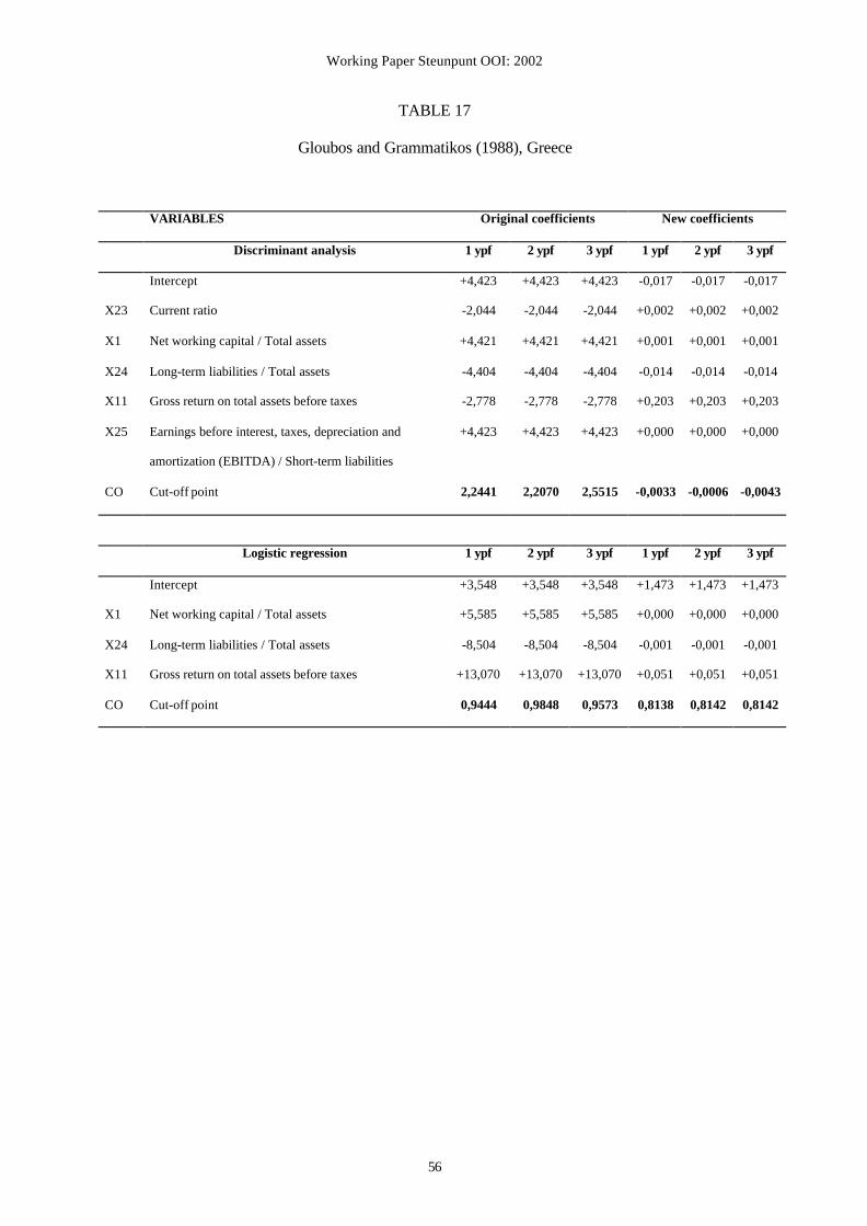
Working Paper Steunpunt OOI: 2002
56
TABLE 17
Gloubos and Grammatikos (1988), Greece
VARIABLES Original coefficients New coefficients
Discriminant analysis 1 ypf 2 ypf 3 ypf 1 ypf 2 ypf 3 ypf
X23
X1
X24
X11
X25
Intercept
Current ratio
Net working capital / Total assets
Long-term liabilities / Total assets
Gross return on total assets before taxes
Earnings before interest, taxes, depreciation and
amortization (EBITDA) / Short-term liabilities
+4,423
-2,044
+4,421
-4,404
-2,778
+4,423
+4,423
-2,044
+4,421
-4,404
-2,778
+4,423
+4,423
-2,044
+4,421
-4,404
-2,778
+4,423
-0,017
+0,002
+0,001
-0,014
+0,203
+0,000
-0,017
+0,002
+0,001
-0,014
+0,203
+0,000
-0,017
+0,002
+0,001
-0,014
+0,203
+0,000
CO Cut-off point 2,2441 2,2070 2,5515 -0,0033 -0,0006 -0,0043
Logistic regression 1 ypf 2 ypf 3 ypf 1 ypf 2 ypf 3 ypf
Intercept +3,548 +3,548 +3,548 +1,473 +1,473 +1,473
X1 Net working capital / Total assets +5,585 +5,585 +5,585 +0,000 +0,000 +0,000
X24 Long-term liabilities / Total assets -8,504 -8,504 -8,504 -0,001 -0,001 -0,001
X11 Gross return on total assets before taxes +13,070 +13,070 +13,070 +0,051 +0,051 +0,051
CO Cut-off point 0,9444 0,9848 0,9573 0,8138 0,8142 0,8142
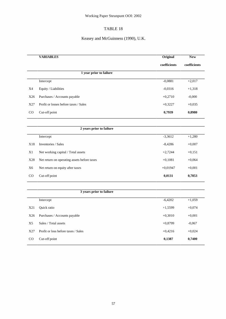
Working Paper Steunpunt OOI: 2002
57
TABLE 18
Keasey and McGuinness (1990), U.K.
VARIABLES Original
coefficients
New
coefficients
1 year prior to failure
Intercept -0,0881 +2,017
X4 Equity / Liabilities -0,0316 +1,318
X26 Purchases / Accounts payable +0,2710 -0,000
X27 Profit or losses before taxes / Sales +0,3227 +0,035
CO Cut-off point 0,7939 0,8980
2 years prior to failure
Intercept -3,3612 +1,280
X18 Inventories / Sales -8,4286 +0,007
X1 Net working capital / Total assets +2,7244 +0,151
X28 Net return on operating assets before taxes +0,1081 +0,064
X6 Net return on equity after taxes +0,01947 +0,001
CO Cut-off point 0,0131 0,7853
3 years prior to failure
Intercept -6,4202 +1,059
X21 Quick ratio +1,5599 +0,074
X26 Purchases / Accounts payable +0,3010 +0,001
X5 Sales / Total assets +0,8799 -0,067
X27 Profit or loss before taxes / Sales +0,4216 +0,024
CO Cut-off point 0,1387 0,7400
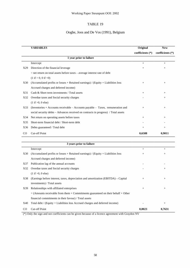
Working Paper Steunpunt OOI: 2002
58
TABLE 19
Ooghe, Joos and De Vos (1991), Belgium
VARIABLES Original
coefficients (*)
New
coefficients (*)
1 year prior to failure
Intercept + +
X29 Direction of the financial leverage
= net return on total assets before taxes – average interest rate of debt
(1 if > 0, 0 if <0)
+ +
X30 (Accumulated profits or losses + Retained earnings) / (Equity + Liabilities less
Accrued charges and deferred income)
+ +
X31 Cash & Short term investments / Total assets + +
X32 Overdue taxes and Social security charges
(1 if >0, 0 else)
- +
X33 (Inventories + Accounts receivable – Accounts payable – Taxes, remuneration and
social security debts – Advances received on contracts in progress) / Total assets
+ +
X34 Net return on operating assets before taxes + +
X35 Short-term financial debt / Short-term debt - -
X36 Debts guaranteed / Total debt + +
CO Cut-off Point 0,6588 0,9011
3 years prior to failure
Intercept + +
X30 (Accumulated profits or losses + Retained earnings) / (Equity + Liabilities less
Accrued charges and deferred income)
+ +
X37 Publication lag of the annual accounts - -
X32 Overdue taxes and Social security charges
(1 if >0, 0 else)
- +
X38 (Earnings before interest, taxes, depreciation and amortization (EBITDA) – Capital
investments) / Total assets
+ +
X39 Relationships with affiliated enterprises
= (Amounts receivable from them + Commitments guaranteed on their behalf + Other
financial commitments in their favour) / Total assets
+ +
X40 Total debt / (Equity + Liabilities less Accrued charges and deferred income) - +
CO Cut-off Point 0,8023 0,7631
(*) Only the sign and not coefficients can be given because of a licence agreement with Graydon NV
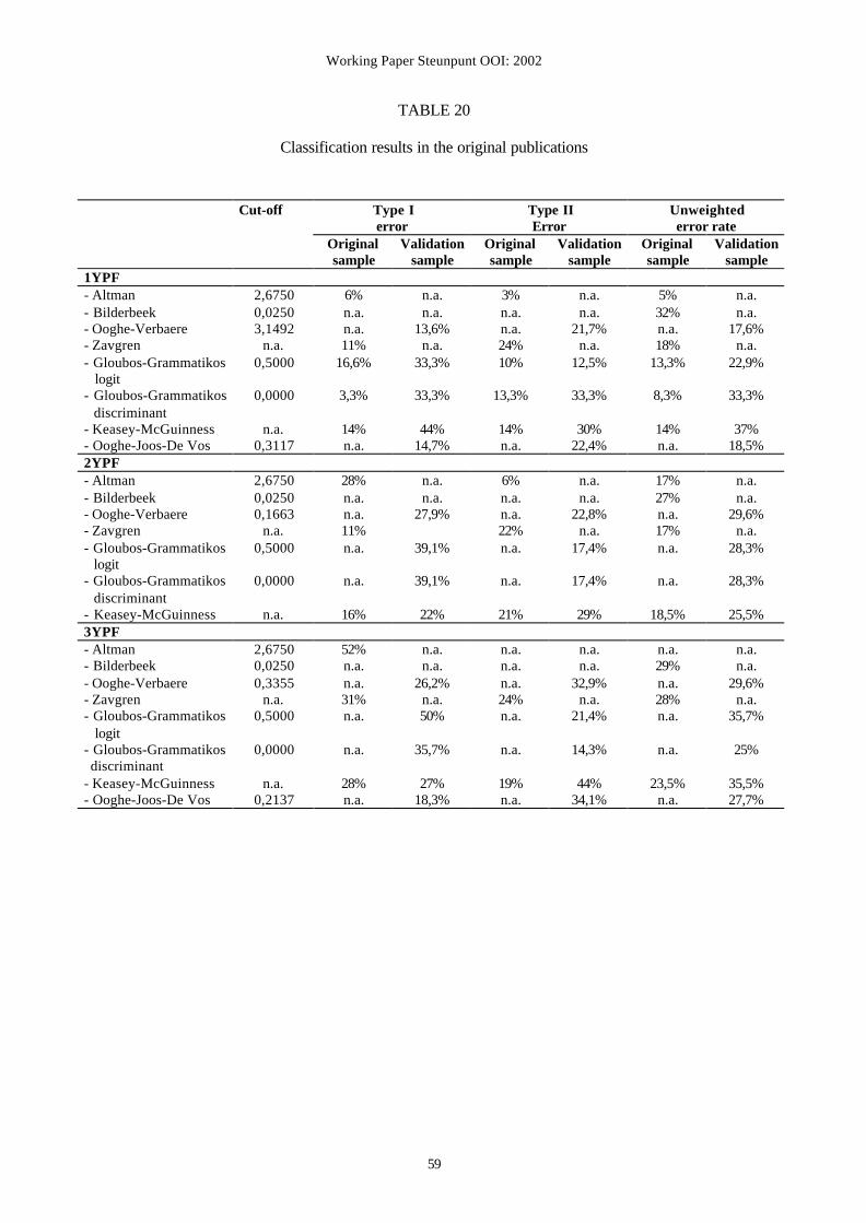
Working Paper Steunpunt OOI: 2002
59
TABLE 20
Classification results in the original publications
Cut-off Type Ierror
Type IIError
Unweightederror rate
Originalsample
Validationsample
Originalsample
Validationsample
Originalsample
Validationsample
1YPF- Altman- Bilderbeek- Ooghe-Verbaere- Zavgren- Gloubos-Grammatikos logit- Gloubos-Grammatikos
discriminant- Keasey-McGuinness- Ooghe-Joos-De Vos
2,67500,02503,1492
n.a.0,5000
0,0000
n.a.0,3117
6%n.a.n.a.11%
16,6%
3,3%
14%n.a.
n.a.n.a.
13,6%n.a.
33,3%
33,3%
44%14,7%
3%n.a.n.a.24%10%
13,3%
14%n.a.
n.a.n.a.
21,7%n.a.
12,5%
33,3%
30%22,4%
5%32%n.a.18%
13,3%
8,3%
14%n.a.
n.a.n.a.
17,6%n.a.
22,9%
33,3%
37%18,5%
2YPF- Altman- Bilderbeek- Ooghe-Verbaere- Zavgren
- Gloubos-Grammatikoslogit
- Gloubos-Grammatikosdiscriminant
- Keasey-McGuinness
2,67500,02500,1663
n.a.0,5000
0,0000
n.a.
28%n.a.n.a.11%n.a.
n.a.
16%
n.a.n.a.
27,9%
39,1%
39,1%
22%
6%n.a.n.a.22%n.a.
n.a.
21%
n.a.n.a.
22,8%n.a.
17,4%
17,4%
29%
17%27%n.a.17%n.a.
n.a.
18,5%
n.a.n.a.
29,6%n.a.
28,3%
28,3%
25,5%3YPF- Altman- Bilderbeek- Ooghe-Verbaere- Zavgren- Gloubos-Grammatikos logit- Gloubos-Grammatikos discriminant- Keasey-McGuinness- Ooghe-Joos-De Vos
2,67500,02500,3355
n.a.0,5000
0,0000
n.a.0,2137
52%n.a.n.a.31%n.a.
n.a.
28%n.a.
n.a.n.a.
26,2%n.a.50%
35,7%
27%18,3%
n.a.n.a.n.a.24%n.a.
n.a.
19%n.a.
n.a.n.a.
32,9%n.a.
21,4%
14,3%
44%34,1%
n.a.29%n.a.28%n.a.
n.a.
23,5%n.a.
n.a.n.a.
29,6%n.a.
35,7%
25%
35,5%27,7%
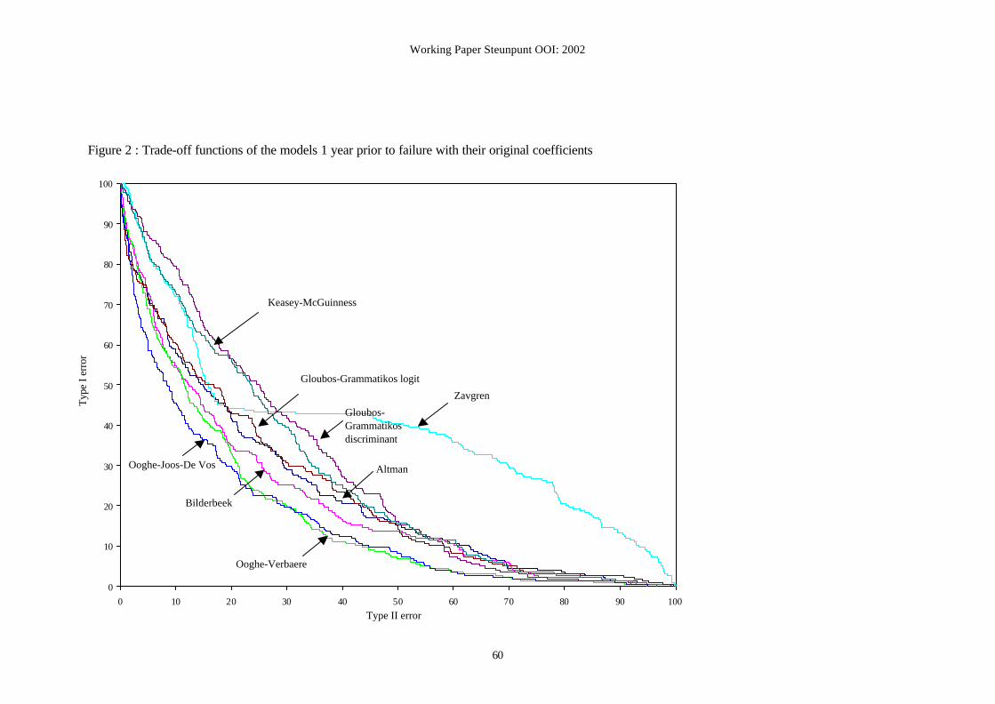
Working Paper Steunpunt OOI: 2002
60
Figure 2 : Trade-off functions of the models 1 year prior to failure with their original coefficients
0
10
20
30
40
50
60
70
80
90
100
0 10 20 30 40 50 60 70 80 90 100
Zavgren
Gloubos-Grammatikos discriminant
Keasey-McGuinness
Gloubos-Grammatikos logit
Bilderbeek
Ooghe-Joos-De Vos
Ooghe-Verbaere
Type
I er
ror
Type II error
Altman

Working Paper Steunpunt OOI: 2002
61
Figure 3 : Trade-off functions of the models 2 years prior to failure with their original coefficients
0
10
20
30
40
50
60
70
80
90
100
0 10 20 30 40 50 60 70 80 90 100
Type II error
Typ
e I
erro
r
BilderbeekOoghe-Verbaere
Gloubos-Grammatikos logit
Altman
Keasey-McGuinness
Gloubos-Grammatikos discriminant Zavgren
Altman

Working Paper Steunpunt OOI: 2002
62
Figure 4 : Trade-off functions of the models 3 years prior to failure with their original coefficients
0
10
20
30
40
50
60
70
80
90
100
0 10 20 30 40 50 60 70 80 90 100
Type II error
Type
I er
ror
Altman
Gloubos-Grammatikos logit
Keasey-McGuinness
Gloubos-Grammatikos discriminant
Ooghe-Verbaere
Bilderbeek
Zavgren
Ooghe-Joos-De Vos
Figure 5 : Trade-off functions of the models 1 year prior to failure with their re-estimated coefficients
0
10
20
30
40
50
60
70
80
90
100
0 10 20 30 40 50 60 70 80 90 100
Keasey-McGuinness
Ooghe-Joos-De Vos
Gloubos-Grammatikos discriminant
Gloubos-Grammatikos logit
Type II error
Typ
e I e
rror
Zavrgen
Bilderbeek
Ooghe-Verbaere
Altman

Working Paper Steunpunt OOI: 2002
63
Figure 6 : Trade-off functions of the models 2 years prior to failure with their re-estimated coefficients
0
10
20
30
40
50
60
70
80
90
100
0 10 20 30 40 50 60 70 80 90 100
Type
I er
ror
Type II error
Gloubos-Grammatikos discriminant
Keasey-McGuinness
Gloubos-Grammatikos logit
Ooghe-Verbaere
Zavgren
Altman
Bilderbeek

Working Paper Steunpunt OOI: 2002
64
Figure 7 : Trade-off functions of the models 3 years prior to failure with their re-estimated coefficients
0
10
20
30
40
50
60
70
80
90
100
0 10 20 30 40 50 60 70 80 90 100
Typ
e I e
rror
Type II error
Gloubos-Grammatikos discriminant
Gloubos-Grammatikos logit
Zavgren
Keasey-McGuinness
Ooghe-Joos-De Vos
Altman
Ooghe-Verbaere
Bilderbeek