are emerging market currency crises predictable? a test

WORKING PAPER SER IES

ISSN 1561081-0

9 7 7 1 5 6 1 0 8 1 0 0 5

NO. 571 / JANUARY 2006

ARE EMERGING MARKET CURRENCY CRISES PREDICTABLE?

A TEST

by Tuomas A. Peltonen

In 2006 all ECB publications will feature

a motif taken from the

€5 banknote.

WORK ING PAPER SER IE SNO. 571 / JANUARY 2006

ARE EMERGING MARKET CURRENCY

CRISES PREDICTABLE?

A TEST 1

by Tuomas A. Peltonen 2

1 This paper is part of the author’s graduate research at the European University Institute, Florence, Italy. The views expressed in this paper are those of the author’s alone and do not necessarily reflect those of the European Central Bank. I am grateful to

Professors Michael Artis, Anindya Banerjee and Karl Schlag and Dr. Jouko Vilmunen for their supervision and comments. Special thanks to Aaron Mehrotra for many fruitful discussions. Comments from an anonymous referee and conference participants at

CESifo-Delphi conference „Global Economic Imbalances: Prospects and Remedies“ in Munich on 11-12 November 2005 helped me to improve this paper. All the remaining errors are mine.

2 European Central Bank, Postfach 16 03 19, 60066 Frankfurt am Main, Germany; e-mail: [email protected]

This paper can be downloaded without charge from http://www.ecb.int or from the Social Science Research Network

electronic library at http://ssrn.com/abstract_id=872529.

© European Central Bank, 2006

AddressKaiserstrasse 2960311 Frankfurt am Main, Germany

Postal addressPostfach 16 03 1960066 Frankfurt am Main, Germany

Telephone+49 69 1344 0

Internethttp://www.ecb.int

Fax+49 69 1344 6000

Telex411 144 ecb d

All rights reserved.

Any reproduction, publication andreprint in the form of a differentpublication, whether printed orproduced electronically, in whole or inpart, is permitted only with the explicitwritten authorisation of the ECB or theauthor(s).

The views expressed in this paper do notnecessarily reflect those of the EuropeanCentral Bank.

The statement of purpose for the ECBWorking Paper Series is available fromthe ECB website, http://www.ecb.int.

ISSN 1561-0810 (print)ISSN 1725-2806 (online)

3ECB

Working Paper Series No. 571January 2006

CONTENTS

Abstract 4

Non-technical summary 5

1 Introduction 6

2 A brief review of the literature 8

3 Methodological issues 9

3.1 Definition of the crisis 9

3.2 The data 10

4 Empirical frameworks 13

4.1 Probit model 13

4.2 General about artificial neural networks 14

4.3 ANN model specification 15

5 Empirical results 17

5.1 Factors affecting to currency crisis 17

5.2 Issues related to crisis prediction 18

5.3 Predicting currency crises 19

5.4 Robustness of results 22

6 Conclusion 22

References 23

7 Appendix 27

7.1 Data sources and transformations 27

7.2 Descriptive statistics 28

7.3 Factors affecting to currency crisis 29

7.4 In-sample forecasts of currency crisisprobabilities 30

7.5 Out-of-sample forecasts of currency crisisprobabilities 32

7.6 Goodness-of-fit measures 33

7.7 Comparison of results 34

7.8 Graphs of in- and out-of-sample forecasts 35

47European Central Bank Working Paper Series

Abstract

This paper analyzes the predictability of emerging market currencycrises by comparing the often used probit model to a new method, namelya multi-layer perceptron artificial neural network (ANN) model. Accord-ing to the results, both models were able to signal currency crises rea-sonably well in-sample, but the forecasting power of these models out-of-sample was found to be rather poor. Only in the case of Russian (1998)crisis were both models able to signal the crisis well in advance. The re-sults reinforced the view that developing a stable model that can predictor even explain currency crises is a challenging task.

JEL classification: F31, E44, C25, C23, C45Keywords: Currency crises, emerging markets, artificial neural networks

4ECBWorking Paper Series No. 571January 2006

Non-technical summaryThis paper investigates the predictability of emerging market currency crises

by comparing two non-linear models. In particular, the paper discusses the ca-pacity of a probit model and a multi-layer perceptron artificial neural network(ANN) model to predict currency crises with a sample of commonly used emerg-ing market countries and crisis indicators. The main contribution of the paper isthat it introduces a new method for currency crisis prediction, namely the ANNmodel. Similar types of ANN models have been successfully used in other fieldsof economics and finance to detect binary outcomes, such as firm bankruptcies.In addition, currency crises determinants and their stability are evaluated us-ing different subsamples to see whether currency crises of 1980s and 1990s werecaused by the same factors. Finally, the impact of a de facto exchange rateregime on the probability of currency crises is evaluated using the data fromReinhart and Rogoff (2004).The main result of the study is that both the probit and the ANN model

were able to correctly signal crises reasonably well in-sample, and that the ANNmodel slightly outperformed the probit model. In contrast to the findings inthe earlier literature on currency crises, the ability of the models to predictcurrency crises out-of-sample was found to be weak. Only in the case of theRussian crisis (1998) were both models able to signal its occurrence well inadvance. In addition, certain economic factors were found to be related to theemerging market currency crises. These factors are the contagion effect, theprevailing de facto exchange rate regime, the current account and governmentbudget deficits, as well as real GDP growth. Furthermore, it appears thateconomic fundamentals were able to statistically better explain the onset ofcurrency crises in the subsample of the 1980s than in the subsample of the 1990s,where other variables, such as the contagion effect, were statistically significant.This confirms earlier findings in the literature that the contagion effect versuseconomic fundamentals might have played a greater role in the onset of thecurrency crises in the 1990s, in contrast to the crises of the 1980s. Furthermore,our findings confirmed the results of Rogoff et al. (2003) and Ghosh et al. (2002)that emerging markets with more rigid exchange rate regimes were less prone tocurrency crises during the last two decades. Finally, the results reinforced theview that developing a stable model capable of predicting currency crises canbe a challenging task.

5ECB


1 IntroductionAccording to Bordo et al. (2001), the frequency of financial crises has doubledsince the collapse of the Bretton Woods system in 1973, but there is littleevidence that crises have become more severe in terms of output losses anddurations. Furthermore, both the IMF (1998) and Bordo et al. (2001) reportthat low-income economies have experienced more banking and currency crisesthan advanced economies during this time. Similar conclusions are drawn inGhosh et al. (2002), who also find that currency crises are more prevalent underde jure floating exchange rate regimes. Likewise, Rogoff et al. (2003) find that,especially in emerging markets, currency crises have occurred during the lastthree decades more often under de facto less rigid exchange rate arrangements,such as the managed floating exchange rate regime. In contrast, they find thattwin crises (both banking and currency crises) occurred more often under defacto pegged exchange rate arrangements.The unfortunate feature of currency crises, and more generally, financial

crises is that they can be very costly. These costs include fiscal and quasi-fiscalcosts, misallocation and an underutilization of resources, losses in real outputand changes in distribution of wealth. Bordo et al. (2001) estimate that thedownturns following financial crises have lasted on average 2-3 years and cost 5-10 per cent of GDP. However, Ghosh et al. (2002) report that costs of currencyand banking crises have varied depending on the exchange rate regime.1 Thismotivates the study as it is important to investigate the causes of past currencycrises and ways of detecting countries vulnerable to crises.In the spirit of Berg and Pattillo (1999),2 who investigated the predictability

of emerging markets currency crises by comparing a ’signal’ approach proposedby Kaminsky et al. (1998) and a probit model, this paper analyzes the pre-dictability of emerging market currency crises comparing two different models.More specifically, the paper discusses the capacity of often used probit/logitmodels to predict currency crises with a sample of commonly used emergingmarket countries and crisis indicators. Furthermore, the main contribution ofthe paper is that it introduces a new method for currency crisis prediction,namely a multi-layer perceptron artificial neural network (ANN) model. Simi-lar types of ANN models have successfully been used in other fields of economicsand finance to detect binary outcomes, such as firm bankruptcies.3 In addition,currency crises determinants and their stability are evaluated using differentsubsamples to see whether currency crises of 1980s and 1990s were caused bythe same factors.4 Finally, the impact of a de facto exchange rate regime onthe probability of currency crises is evaluated using the data from Reinhart andRogoff (2004).5

1Ghosh et al. (2002) found that, in their sample, per capita GDP growth rate underfloating exchange rate regime was faster after currency crises than before them. However,under fixed or intermediate exchange rate regimes, crises caused substantial declines in percapita GDP growth rates.

2 See also Edison (2003).3 See e.g. a survey by Wong and Selvi (1998).4One should note that in many of the analyzed economies, the capital accounts were

liberalized at the early 1990s.5Also Rogoff et al. (2003) evaluated this using the same data, however their approach

was different as they only tabulated the occurance of currency crises under different de factoexchange regimes without conditioning the probability of currency crises on other factors like


in this study.

According to currency crisis theories, economic fundamentals affect the prob-ability of currency crises. However, whether the exact timing of a currency crisisis predictable is another issue. According to the first generation models of cur-rency crisis,6 the exact timing of currency crisis is linearly determined by, andtherefore, predictable with economic fundamentals. In contrast, in the secondgeneration models of currency crisis,7 economic fundamentals also affect theprobability of crisis, but the relationships can be non-linear. Furthermore, otherfactors than economic fundamentals, such as ’herding behaviour’ and other typesof investor behaviour, can affect the probability of crisis. Therefore, it may notbe possible to predict the exact timing of crisis solely by economic fundamentals.However, the possible non-linear relationship between economic fundamentalsand currency crises motives the use of non-linear methods, such as probit/logitor ANN models for empirical analyses of currency crisis. Thus, it also motivatesthe study to analyze whether the more advanced ANN model could outperformthe standard probit model in currency crisis prediction.However, there is an important issue of endogeneity linked to the currency

crises. Consider that economic agents follow an economic indicator that is ex-pected to be linked to currency crises. Thus, crises can either be prevented dueto policy changes or, in contrast, they can erupt due to ’self-fulfilling prophe-cies’. Furthermore, not all currency crises are caused by the same factors, andother issues, such as political factors, can also play a role in the onset of cur-rency crises. Another problem related to currency crisis prediction, especiallyin emerging markets, is linked to the availability of timely and accurate in-formation about economic fundamentals and other relevant factors, as well asindicators that contain information about investors’ expectations about futureeconomic conditions. Despite these issues, many earlier studies have claimed tobe successful in predicting currency crises using economic fundamentals, whichwill also be the focus of this study.The main result of the study is that both the probit and the ANN model

were able to correctly signal crises reasonably well in-sample, and that the ANNmodel slightly outperformed the probit model. In contrast to the findings in theearlier currency crises literature, the ability of the models to predict currencycrises out-of-sample was found to be weak. Only in the case of the Russian(1998) crisis were both models were able to signal its occurrence well in advance.In addition, certain economic factors were found to be related to the emergingmarket currency crises. These factors are the contagion effect, the prevailingde facto exchange rate regime, the current account and government budgetdeficits, as well as real GDP growth. Furthermore, it appears that economicfundamentals were able to statistically better explain the onset of currencycrises in the subsample of the 1980s than in the subsample of the 1990s, whereother variables, such as the contagion effect, were statistically significant. Thisconfirms the earlier findings in the literature that the contagion effect versuseconomic fundamentals might have played a greater role in the onset of thecurrency crises in the 1990s, in contrast to the crises of the 1980s. This result ispossibly linked to the fact that many of the analyzed emerging market economiesliberalized their capital accounts in the beginning of the 1990s, which possiblymade them more vulnerable to international capital flows than they were in

6See Krugman (1979).7 See Obstfeld (1986, 1995).

7ECB


the 1980s. Furthermore, our findings confirmed the results of Rogoff et al.(2003) and Ghosh et al. (2002) that emerging markets with more rigid exchangerate regimes were less prone to currency crises during the last two decades.Finally, the results reinforced the view that developing a stable model capableof predicting or even explaining currency crises can be a challenging task.The study is organized in the following way. Section Two briefly summarizes

the related literature. Section Three discusses methodological issues, while sec-tion Four presents the empirical framework. Section Five presents the resultsand, finally, section Six concludes.

2 A brief review of the literatureBefore the financial crises of the 1990s, it was commonly held that currencycrises could be, to some extent, predictable with variables derived from the firstgeneration models of currency crisis stemming from Krugman (1979).8 Authorssuch as Blanco and Garber (1986), Cumby and van Wijnbergen (1989), Edwards(1989) and Goldberg (1994) explored the Latin American currency crises ofthe 1980s, for example the devaluations in Mexico (1982, 1986) and Argentina(1981). They found that variables such as current account and governmentbudget balances, credit growth, foreign reserves, inflation, and real exchangerates were related to currency crises.In the early 1990s, there were several financial and currency crises, e.g.

the EMS crisis of 1992-93, which could not be explained using the argumentsfrom first generation models of currency crisis. This led to the developmentof second generation models of currency crisis originating from Obstfeld (1986,1995).9 Furthermore, it again raised the question whether currency crises couldbe predicted with economic fundamentals. To tackle the problem, Eichengreenet al. (1995), Sachs et al. (1995) and Kaminsky et al. (1996), among others,introduced models with a broader set of explanatory variables. Kaminsky etal. (1996) summarized the results of a large number of earlier studies andfound that the following variables had the greatest predictive power of currencycrises: inflation, GDP growth, exports, real exchange rate misalignment, moneygrowth, reserves, credit growth, credit to the public sector, fiscal deficit and M2to reserves ratio. In addition, current account, short-term debt to reserves ratio,stock market growth, lending boom (credit to private sector to GDP) and theworld interest rate were found to be related to currency crises.The Asian crises of 1997-98 motivated the development of third genera-

tion currency crises models with financial issues from both banks’ and firms’side being the key elements. Concepts such as the ’over-borrowing syndrome’,’crony capitalism’, and ’moral hazard lending’ became known from papers suchas McKinnon and Pill (1996), Chang and Velasco (1998), Krugman (1999),Aghion et al. (2001, 2004) and Burnside et al. (2004). In addition to economicfundamentals related to currency crises, models explaining the propagation ofcrises, i.e. contagion effects have been studied extensively, see e.g. Forbes andRigobon (2002).In the empirical works on currency crisis, the binary crisis variable is usually

related to the explanatory variables or ’leading indicators’ in different ways.

8Agenor et al. (1991) review these models.9Flood and Marion (1998) review this literature.


Firstly, the most often used method is a binary choice model, like the pro-bit/logit model. Examples of these studies are e.g. Eichengreen et al. (1995,1996) and Frankel and Rose (1996). Recently, Berg and Pattillo (1999), Ko-mulainen and Lukkarila (2003) and Kumar et al. (2003) have also analyzedthe predictability of emerging market currency crises using probit/logit models,whereas Bussière and Fratzscher (2002) used a more sophisticated multinomiallogit model. All these studies conclude that certain economic fundamentals(from the variables mentioned earlier) can explain currency crises, and the crisesof the 1980s and the 1990s would have been, at least to some extent, predictable.Secondly, the other method is to consider the predictive power of the variablesone at a time (univariate) so that a variable is considered to be a good leadingindicator if it gives a correct signal of crisis before the incident. This ’signal’approach, or ’early warning indicator system’, was introduced by Kaminsky etal. (1996, 1998), and further developed by Edison (2003) and Kaminsky (2003).Finally, other recent approaches analyzing currency crises have been Fisher’slinear discriminant analysis by Burkart and Coudert (2002), a duration modelanalysis by Tudela (2004), and an analysis using ANN models by Frank andSchmied (2003).10 In addition, Scott (2000) explored contagion effects applyingan ANN model to Asian crisis countries.

3 Methodological issues

3.1 Definition of the crisis

In this study, currency crises are defined using the concept of ’exchange mar-ket pressure’ by Girton and Roper (1977). This way of defining crises has anadvantage over the alternative definitions of currency crisis, which rely only onextreme currency movements, because both ’successful’ and ’unsuccessful’ spec-ulative attacks can be considered.11 In addition, the ’exchange market pressure’definition of crises has the appeal that it can be used to analyze speculative at-tacks under both fixed and flexible exchange rate regimes.Following earlier studies,12 the exchange market pressure in a country i at

time t can be measured as:

EMPi,t = [α%∆ei,t − β%∆ri,t] (1)

where ei,t denotes the price of a U.S. Dollar in the country i’s currency at thetime t; ri,t denotes the foreign reserves (excluding gold) of country i at thetime t and α and β are the weights that equalize the variances of these twocomponents.

10A study by Franck and Schmied (2003) uses a very similar type of ANN model to predictRussian (1998) and Brazilian (1999) crises. However, their analysis is more event study typeand does not compare the results to an alternative statistical model like this study.11The ’successful’ speculative attack means occassions where the currency in consideration

depreciates/appreciates strongly. The ’unsuccessful’ speculative attacks means occassions,where the central bank has been able to defend the currency (i.e. the currency has not beendevalued/revalued) by intervening in the foreign exchange markets.12 Sometimes the exchange market pressure index also includes a term consisting of short

interest rate differential to the US. This term is, however, omitted here due to data problems,as in many emerging market economies a representative market determined money marketinterest rate is available only from the mid-1990s onwards.

9ECB


The first term, α%∆ei,t, measures the percentage change of the price ofa U.S. Dollar in the country i’s currency at the time t; in another words, itmeasures the devaluation (or revaluation) rate of the nominal exchange rate ofthe country i. The second term, β%∆ri,t, measures the percentage change inthe level of the country i’s foreign reserves. It has a negative sign because adecrease in the foreign reserves is assumed to reflect foreign currency outflows(weakening pressure of the local currency i) that the central bank attempts tolimit by intervening (buying the local currency) in the foreign exchange market.Therefore, a positive value of the exchange market pressure index measuresthe depreciation pressure of the currency i, while a negative value of the indexmeasures the appreciation pressure of the currency i.A currency crisis is defined as an extreme value of the exchange market

pressure index:

Crisisi,t = 1, if EMPi,t > µEMPi + 2.0σEMPi (2)

Crisisi,t = 0, otherwise (3)

where µEMPi and σEMPi are the sample mean and the standard deviation ofthe exchange market pressure index for each country i. Furthermore, currencycrises occurring within three months were considered as one crisis. This methodof detecting speculative attacks and currency crises is widely used in the em-pirical works although it has faced some criticism, mostly because of its ad hocnature and due to the lack of a direct role of market expectations. To test therobustness of the results, alternative crisis definitions were also constructed.This is explained in more detail in section 5.4.

3.2 The data

The dataset consists of 24 commonly used emerging market countries,13 namely:Argentina, Brazil, Chile, Colombia, Czech Republic, Ecuador, Egypt, Hungary,India, Indonesia, Israel, Korea, Malaysia, Mexico, Morocco, Peru, Philippines,Poland, Russia, Slovakia, South Africa, Thailand, Turkey, and Venezuela. Thetime span of the monthly dataset was 12/1980 — 12/2001. However, in mostcases, the data was not available for the whole time period and the actualdataset that was used in estimations was unbalanced and had a maximum of3706 observations. The dataset already ends by 12/2001, because the data forthe de facto currency regime classification by Reinhart and Rogoff (2004) wasnot available for later periods. Furthermore, as Reinhart and Rogoff (2004)show, there is a significant difference between the IMF’s de jure classificationand the de facto classification of exchange rate regimes, especially in the hyper-inflationary periods of 1980s. Therefore, it was considered important to includethe de facto exchange rate regime into the analysis with the cost of losing someof the latest observations.14 Other data sources were: the IMF InternationalFinancial Statistics 2/2005, J.P. Morgan (for real effective exchange rates), and

13The coverage of countries in the Morgan Stanley Capital International (MSCI) EmergingMarkets (EM) index is nearly identical to the sample of countries that is used in this study. Inaddition to the countries in the sample, the EM index also includes China, Jordan, Pakistan,and Taiwan. However, it does not include Ecuador and Slovakia.14This is clearly a drawback as e.g. the floating of Venezuela’s crawling peg regime in

January 2002 and Argentina’s currency board system in February 2002 cannot be investigated.


Global Financial Data Inc. (for stock market indices). The choice of the in-dependent variables was based on theoretical models of currency crisis, whichaim to measure domestic and external conditions15 of the economy. In addition,all used variables have also been found to be related to currency crises in theearlier empirical literature reviewed in section 3.2. Table 1 summarizes the in-dependent variables and more information about the data can be found in theAppendix.

Independent variables FormulaRatio of government budget balance to GDP IFS line 80 / IFS line 99BRatio of current account to GDP IFS line 78ALD / (IFS line 99B / IFS line AE)Measure of under or overvaluation of Real Effective Exchange Rate (REER - HP trend of REER with a parameter of 14400) / REERReal interest rate IFS line 60L - IFS line 64.XAnnualized growth rate of real GDP Annualized growth rate[IFS line 99B / IFS line 99BIP]Annualized growth rate of real domestic credit Annualized growth rate[IFS line 32 / IFS line 99BIP]Annualized growth rate of ratio of broad money to foreign reserves Annualized growth rate[((IFS line 34 + IFS line 35) / IFS line AE) / IFS line 1L.D]Annualized growth rate of stock market Annualized growth rate[Composite stock index]Dummy for contagion A currency crisis within 3 months in the same regionDummy for hyperinflation Annual CPI inflation > 40%Dummy for de facto pegged FX regime See Reinhart and Rogoff, 2004Dummy for de facto crawling ped FX regime See Reinhart and Rogoff, 2004Dummy for de facto managed float FX regime See Reinhart and Rogoff, 2004Dummy for de facto floating FX regime See Reinhart and Rogoff, 2004Dummy for de facto freely falling FX regime See Reinhart and Rogoff, 2004Dummy variables for areaLinear and quadratic time trends

Table 1: The independent variables.

On this occasion, it is useful to discuss the data-related issues a bit morein detail. Firstly, as has been the case in many recent papers investigatingthe determinants and/or predictability of the emerging markets currency cri-sis, the frequency of data was chosen to be monthly. This raises an issue, asvariables such as the GDP, current account or government budget balance, areonly available for emerging markets in annual frequency for long enough timeperiods. Therefore, a common feature of many earlier papers has been that an-nual or quarterly variables have been interpolated either linearly or using splinetechniques. In this study, the GDP, current account and government budgetbalance variables were linearly interpolated into monthly series. While usinginterpolated series, some econometrical issues might arise. However, economi-cally, the greatest difficulty of using interpolated series is that by doing so oneuses information about future economic conditions that was not available toeconomic agents at the time. In contrast, it can be argued that economic agentsoften use forecasts of the key economic variables when they make their invest-ment decisions simply because the actual information is not available. Thisissue has been dealt with in earlier papers by lagging the interpolated variables.In this study, the independent variables were lagged by a month16 to alleviatethis problem. Another problem related to the timing of the variables is that ifthe independent variables were contemporaneous to the crisis variable, it would

15 In addition, foreign debt variables (both total and short-term debt as a ratio of foreignreserves and the GDP) were tested. These variables were not, however, taken into the finalmodels as the foreign debt data from BIS-IMF-OECD-World Bank starts only from 6/1990,which would have shorten the sample considerably.16All the models were estimated also using the independent variables lagged by 3 months.

See section 5.4 for more information.

11ECB


be difficult to evaluate the relationship between economic fundamentals and thecurrency crisis.17

Secondly, an important issue that has often been neglected in many ear-lier studies is related to the time series properties of the variables, as both thediscrete choice models and the ANN models18 require stationary variables. Al-though many authors in the field have constructed their independent variablesas ratios to GDP, deviations from a trend or as growth rates, there are econo-metrical problems linked to hyperinflation periods and transition phases. Forexample, the often used variables such as inflation, the ratio of M2 to foreignreserves, nominal interest rate or the interest rate differential to the US, arehighly unlikely to be stationary throughout 1980-2004 in economies with hyper-inflationary periods or transition phases from command to market economies.In some cases, however, the question is not whether the series contains a unitroot; instead, the question is how the structural shifts should be taken intoaccount.In this study, both standard univariate (augmented Dickey and Fuller (1981)

and Phillips and Perron (1981) tests) and panel (Levin et al. 2002 and Im etal., 2003) unit root tests were applied. In all the univariate unit root tests, thenull hypothesis of a unit root was rejected at a minimum of 10 per cent levelof significance in 17 countries in the case of the variable government budgetbalance, in 21 countries in the case of the variable current account to GDP, andin 22 countries in the case of real interest rate. However, both panel unit roottests rejected the null hypothesis that all series are non-stationary against analternative that all series are stationary at a minimum of 10 per cent level ofsignificance in the case of these three variables. In the case of the other variables,both panel unit root tests rejected the null hypothesis at a minimum of 5 percent level of significance. Therefore, the variables used in the regressions wereconsidered to be stationary or trend stationary.The hyperinflationary periods were identified with a dummy variable that

received value one for the months in which the annual inflation rate exceeded40 per cent. This definition is consistent with the freely falling exchange rateregime classification by Reinhart and Rogoff (2004). In contrast to many earlierstudies, the inflation rate was not used as an explanatory variable, as it wasexpected to be integrated of order 1 in most cases. In addition, variables suchas the interest rate, domestic credit and the GDP were expressed as real series.Some studies exclude hyperinflationary periods from their sample. This would,however, limit the sample considerably and also cause some sample selectionissues if the hyperinflationary periods and de facto freely falling exchange rateregimes were left out of study. In contrast to some earlier studies, variables,such as (lagged) changes in foreign reserves or changes in exchange rate wereleft out due to obvious collinearity problems as crises themselves were definedusing these variables. Finally, a dummy variable was generated to proxy forcontagion effects. Namely, this dummy was set to unity when another countryin the same area had experienced a currency crisis within the last three months.

17 It is important to emphasize that this paper does not aim to investigate the causal relation-ships between economic fundamentals and currency crises and therefore the abovementionedrelationships should not be interpreted as causal relationships.18 Some ANN models can be used with non-stationary time series.


4 Empirical frameworks

4.1 Probit model

Consider the binary choice model with a panel data (i = 1, ..., N ; t = 1, ..., T ).The unobservable response variable y∗it can be written in the latent form asfollows:

y∗it = xitβ + uit = xitβ + αi + νit, (4)

where the error term uit is disaggregated to the unobserved effect αi and thegeneral error term νit. The observed binary variable yit is defined by

yit = 1, if y∗i ≥ 0 (5)

yit = 0, otherwise (6)

In the probit model case, the cumulative distribution is a standard normal:

Pr(yit = 1|xi, αi) = Pr(yit = 1|xit, αi) = Φ(xitβ + αi) (7)

The first equality states that xit is assumed to be strictly exogenous conditionalon αi. Another standard assumption is that the outcomes yit = yi1, ..., yiTare independent conditional on (xi, αi). Thus, the density of yit conditional on(xi, αi) can be derived:

f(y1, ..., yT |xi, αi;β) =TYt=1

f(yt|xit, αi;β), (8)

wheref(yt|xt, α;β) = Φ(xtβ + α)yt

£1− Φ(xtβ + α)1−yt

¤(9)

Finally, in a random effects panel framework, the unobserved effect αi condi-tional on xi is expected to be normally distributed with:

αi|xi ∼ N(0, σ2α) (10)

However, the assumption of independency of outcomes (i.e. crisis and tranquilperiods) is limiting and it can be relaxed by using the formula:

Pr(yit = 1|xi) = Pr(yit = 1|xit) = Φ(xitβα) (11)

where βα = β/¡1 + σ2α

¢1/2is estimated from pooled probit of yit on xit using

Huber/White robust standard errors, meaning that the coefficients are averagepartial effects. Another observation is that most of the independent variables aretransformed into growth rates, meaning that if the unobservable effect (countryspecific effect) is expected to be time invariant, it will be removed throughthese variable transformations. Indeed, the likelihood ratio test of αi = 0 aftera random effects probit model could not have been rejected at conventionallevels of significance. This confirmed the chosen approach of estimating themodel using pooled panel. Finally, it should be emphasized that the probit (aswell as the ANN) models were estimated using lagged independent variables,i.e. the probability of crisis at time t was predicted using information at t− 1:Pr(yit = 1|xit−1) for the reasons mentioned above.

13ECB


4.2 General about artificial neural networks

Artificial neural networks (ANN)19 are multivariate nonlinear nonparametricstatistical methods,20 which have been used since the late 1980s in finance ap-plications and lately in many different economics research contexts, as in fore-casting exchange rates, inflation and GDP growth. One of the definitions ofANN is

... a neural network is a system composed of many simple processingelements operating in parallel whose function is determined by networkstructure, connection strengths, and the processing performed at comput-ing elements or nodes. DARPA (1988, 60).

Several distinguishing features of ANNs make them valuable for functionapproximation, forecasting, pattern recognition and classification tasks. Firstly,ANNs are distribution-free methods. Secondly, ANNs are suitable for problemswhere the (economic) relationships are not known from the theory or they aredifficult to specify. An ANN model is normally composed of several layers ofcomputing elements called nodes (or neurons). Each node receives an inputsignal from other nodes or external inputs and then, after processing the sig-nals locally through a transfer function, it outputs a transformed signal to theother nodes or gives the final result. The ANN models are characterized by thenetwork architecture: the structure and number of layers, the number of nodesin each layer, how the layers are connected, and how the network is trained.Many of the above features make the ANN models also subject to criticism.

Firstly, the ability and flexibility of ANN models to fit well to the data oftenraises concerns of ’overfitting’. Secondly, as for many nonlinear models, thereexists no ’closed form’ solutions for the ANN model, which makes it difficultto interpret the coefficients in the way it is done with linear models. Thirdly,in many cases the optimization algorithms of complex non-linear functions aresubject of finding locally optimal solutions instead of globally optimal solutions.Therefore, the ANN models are sometimes called as ’black box’ methods despitetheir sound statistical background.This study utilizes the most often used ANN model called multi-layer per-

ceptron (MLP), where all the nodes and layers are arranged in a feed-forwardmanner (see figure 1). The first layer is called the input layer, where the infor-mation is received in the ANN. Usually the input layer consists of as many inputnodes as there are independent variables. The last layer is called the outputlayer where the ANN produces its solution.21 In between, there are one or morehidden layers, which make the ANN models distinctive from other statisticalmodels. Finally, all nodes in the adjoining layers are connected by acyclic arcsfrom lower to higher layers. Commonly, in the classification studies, one hiddenlayer structure is used referring to the study of Hornik et al. (1989), which showsthat an ANN model with a single hidden layer can approximate any continuousfunction to any desired accuracy. In some cases, however, a two-hidden layer

19See Haykin (1999) for a comprehensive theoretical presentation of ANNs. In addition,McNelis (2005) provides an excellent book of ANN applications.20 See White (1989) for more details.21The output values from these type of ANNs are the estimates of the Bayesian posterior

probabilities.


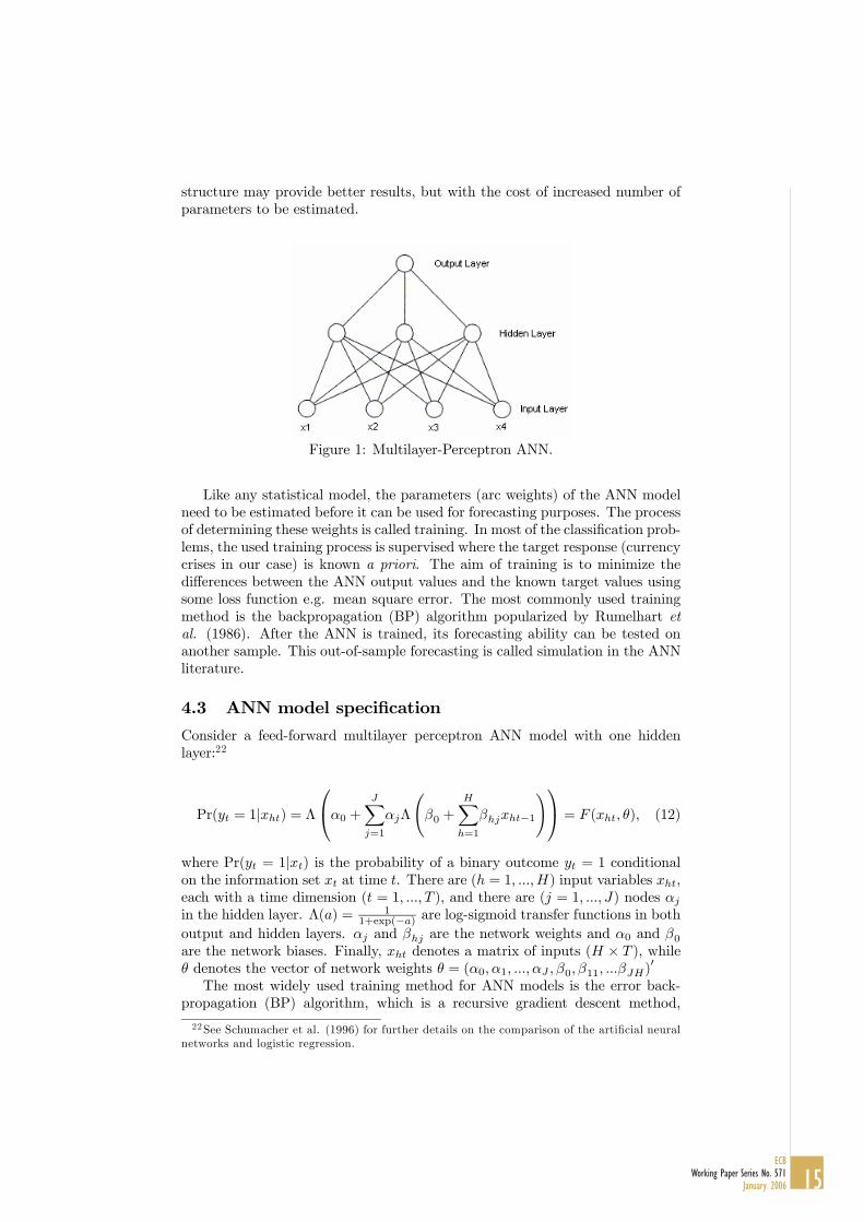
structure may provide better results, but with the cost of increased number ofparameters to be estimated.

Figure 1: Multilayer-Perceptron ANN.

Like any statistical model, the parameters (arc weights) of the ANN modelneed to be estimated before it can be used for forecasting purposes. The processof determining these weights is called training. In most of the classification prob-lems, the used training process is supervised where the target response (currencycrises in our case) is known a priori. The aim of training is to minimize thedifferences between the ANN output values and the known target values usingsome loss function e.g. mean square error. The most commonly used trainingmethod is the backpropagation (BP) algorithm popularized by Rumelhart etal. (1986). After the ANN is trained, its forecasting ability can be tested onanother sample. This out-of-sample forecasting is called simulation in the ANNliterature.

4.3 ANN model specification

Consider a feed-forward multilayer perceptron ANN model with one hiddenlayer:22

Pr(yt = 1|xht) = Λ

⎛⎝α0 +JXj=1

αjΛ

Ãβ0 +

HXh=1

βhjxht−1

!⎞⎠ = F (xht, θ), (12)

where Pr(yt = 1|xt) is the probability of a binary outcome yt = 1 conditionalon the information set xt at time t. There are (h = 1, ...,H) input variables xht,each with a time dimension (t = 1, ..., T ), and there are (j = 1, ..., J) nodes αjin the hidden layer. Λ(a) = 1

1+exp(−a) are log-sigmoid transfer functions in bothoutput and hidden layers. αj and βhj are the network weights and α0 and β0are the network biases. Finally, xht denotes a matrix of inputs (H × T ), whileθ denotes the vector of network weights θ = (α0, α1, ..., αJ , β0, β11, ...βJH)

0

The most widely used training method for ANN models is the error back-propagation (BP) algorithm, which is a recursive gradient descent method,

22See Schumacher et al. (1996) for further details on the comparison of the artificial neuralnetworks and logistic regression.

15ECB


where the network weights θ are chosen to minimize a loss function, typicallythe sum of squared errors:

minθ

L =1

T

TXt=1

(yt − byt)2 , (13)

where yt is the target output, byt is the estimated output value byt = F (xht, θ)with sample size T . The loss function is iterated until its minimum23 is achieved.The iterative step of the algorithm takes θ to θ +∆θ, which is calculated as:

∆θ = −π∇F (xht, θ) (yt − F (xht, θ)) (14)

where π is the learning rate and ∇F (Xht, θ) is the gradient of F (Xht, θ) withrespect to the weight vector θ.The standard backpropagation algorithm is often too slow for practical prob-

lems. Therefore, a notable faster variation of the BP algorithm, namely theLevenberg-Marquardt (LM) algorithm, was used.24 The main difference be-tween the standard BP algorithm and the LM algorithm is that the LM algo-rithm uses an approximation of the Hessian matrix. Otherwise, the networkstructure was the following: First, the choice of the number of nodes in thehidden layer was based on Hannan-Quinn (HQ criteria)25 when the model wasestimated using a different number of nodes (from 2 to 10). The model was cho-sen to be as parsimonious as possible to avoid ’overfitting’ the model to the data,which would have meant a loss of generalization ability of the model. Therefore,the number of nodes in the hidden layer was set to two (j = 2). Second, thelearning rate was kept at its default rate of 0.1 (π = 0.1). Theoretically, a toolarge learning rate would lead to unstable learning, but a too small learningrate would lengthen the estimation time. Third, the models also contained in-put delays in order to take into account the sequential time order of the inputvectors, i.e. the ANN models were constructed as dynamic models. However,the models were trained in a ’batch mode’ with all the input vectors presentedto the network before the weights and biases were adjusted.26 Finally, in orderto compare the forecast capability of the ANN models to the probit models, thesame independent variables (h = 19) and the binary crisis indicator were usedin both cases.23The well-known problems of the backpropagation algorithm are its slowness in convergence

and its inability to escape from local minima.24 In this study, the estimations were repeated several times in order to ensure the conver-

gence of the optimization algoritm. However, ANN model trained with a genetic algoritmcould avoid possible problems related to local minima of the loss function minimization. Thisis left for future study.25Another way of choosing the ANN model is suggested by Anders and Korn (1999). Their

’bottom-up’ strategy starts with a simple network infrastructure and adds hidden nodes oneat a time to the ANN model until cross validation errors of the more complex model becomelarger than with the simpler model.26Adaptive learning machine could be constructed for currency crises purposes. This is left

for future studies.


5 Empirical results

5.1 Factors affecting to currency crisis

Factors affecting the probability of an emerging market currency crisis were es-timated using a probit model with robust standard errors. As mentioned above,the data used was a pooled panel with independent variables lagged by onemonth.27 Table 5 in the Appendix presents the marginal effects (slope coeffi-cients) of the economic factors and exchange rate regimes, as well as contagionand area dummies on the probability of currency crisis. All the variables wereexpressed in natural logarithms with the exception of the real interest rate andthe dummy variables allowing the slope coefficients to be interpreted as elastici-ties. There are four columns in the table: columns 1-3 present the estimates formodels that were used for in-sample predictions, while column 4 shows the es-timates for the model that was used for the out-of-sample predictions. Column1 shows the results for the whole sample of 12/1980 - 12/2001, while columns2 and 3 show the results for the subsamples of 12/1980 - 12/1989 and 1/1990 -12/2001, respectively. Finally, the model in column 4 was estimated using thesample of 12/1980 - 12/1996. The models were estimated using different sub-samples28 to see whether different factors affected the probability of currencycrises in the 1980s and 1990s, and to evaluate the stability of the models. Thisis because, the liberalization of capital accounts in many of the analyzed coun-tries in the early 1990s is expected to have an impact on the crisis dynamics, ascountries have became more exposed to international capital flows.As can be seen from table 2, the signs of the estimated slopes are in line with

currency crisis theories. The economically most significant factors increasing theprobability of currency crises are the proxy for contagion effect, the prevailing defacto exchange rate regime, an increase in the current account and governmentbudget deficits, a decrease in the real GDP growth rate, as well as regionalfactors. According to the results for the whole sample (column 1), the proxyfor contagion effect is found to have the largest marginal effect.29 Namely, acurrency crisis in the same region within three months is estimated to increasethe monthly probability of currency crisis by around 15 per cent. Economically,this effect is significant. In addition, de facto rigid (pegged, crawling peg, andto a lesser extent, managed float) exchange rate regimes are associated with alower probability of currency crises. More specifically, the monthly probabilityof a currency crisis is estimated to decrease by around 2-4 per cent when acountry operates under a rigid exchange rate regime. This result is in line withearlier studies, such as Rogoff et al. (2003) and Ghosh et al. (2002).Turning to other economic factors linked to currency crises, a one per cent

increase in the level of current account and government budget balance (bothto the GDP) is estimated to decrease the monthly probability of currency crisisby around 0.19 per cent and 0.13 per cent, respectively. This means that a onepercentage point increase of both ratios from their sample mean values (-2.1 to-1.1 per cent and -2.7 to -1.7 per cent, respectively) would decrease the monthly

27All models were estimated also using independent variables lagged by 3 months. Theresults remained broadly unchanged and are available on request.28The subsamples for 1980s and 1990s have different number of observations due to missing

observations.29The dummy for contagion effect is statistically significant only with the independent

variables lagged by one month.

17ECB


probability of a currency crisis by around 9.1 and 4.8 per cents, respectively.Similarly, a one per cent increase in the growth rate of real GDP decreasesthe probability of a currency crisis around 0.07 per cent. This means that ifthe annual growth rate of real GDP increases by one percentage point from itssample mean of 4.1 per cent to 5.1 per cent, the monthly probability of currencycrisis would decrease by around 1.7 per cent. Furthermore, Asian countries seemto be statistically more prone to currency crises, while, in contrast, Europeancountries seem to be less so. Finally, the marginal effects of the real interestrate and the growth rate of the ratio of broad money to foreign reserves arestatistically significant, but economically very small.The following observations can be made from the results when the subsam-

ples were used (columns 2 and 3). Firstly, it appears that economic funda-mentals30 could statistically better explain the onset of currency crises in thesubsample of the 1980s than in subsample of the 1990s.31 Specifically, morevariables from the traditional currency crisis theories seem to be statisticallysignificant in column 2, while in column 3 other variables, such as dummyvariables for contagion effect and exchange rate regimes, are statistically signifi-cant.32 In addition, the model for the 1980s subsample has higher goodness-of-fitmeasures, such as the Pseudo R-square. This confirms earlier findings in theliterature that the contagion effect versus economic fundamentals might haveplayed a larger role in the onset of the currency crises in the 1990s. In addi-tion, this also indicates that the liberalization of capital accounts in many ofthe analyzed countries in the early 1990s has possibly made them more vulner-able to international capital flows than they were in the 1980s. Furthermore,a regional dummy variable for Asia has a positive and statistically significantmarginal effect in the sample of the 1990s, while a regional dummy variable forLatin America has a negative and statistically significant marginal effect in thesample of the 1980s. Finally, the slope coefficients of the model in column 4 arein line with the findings from the other subsamples.To sum up, the analysis shows that certain economic variables were associ-

ated with the currency crises of the 1980s and the 1990s, and can have statisti-cally and economically significant impact on the probability of currency crises.It seems that in the 1980s economic fundamentals derived from the currencycrisis theories were capable of explaining the onset of the currency crises. Incontrast, in the 1990s, other factors, such as the contagion effect and the defacto currency regimes, seem to have played a larger role in the occurrence ofcurrency crises. This reinforces the view that developing a stable model thatcould predict or even explain currency crises can be challenging.

5.2 Issues related to crisis prediction

The ability of models to predict currency crises was evaluated using cross-tabulations of correct classifications, as well as different goodness-of-fit mea-sures, such as Brier’s Quadratic Probability Score (QPS), the Receiver Operat-30Also hyperinflation dummy was found to be statistically and economically significant for

the 1980s subsample.31 It should be noted that in both subsamples, the share of crisis periods was roughly the

same: 3.66 percent in the 1980s subsample and 3.72 percent in the 1990s subsample.32When the model was estimated using the subsample of the 1990s and using the inde-

pendent variables lagged one period (column 3), the marginal effect of currency crisis in theregion was estimated to be 0.18 (18 percent).


ing Characteristic (ROC) and Cramer’s Gamma. In addition, the in-sample andout-of-sample predicted probabilities for the countries were plotted to illustratethe ability of the models to predict crisis.Certain issues are related to the evaluation of the predictive ability of the

models. First, in the binary choice models, the choice of the probability thresh-old is critical. As Greene (2000, 833) states, the usual threshold value of 50per cent may not be a good value if the binary outcomes in the sample are un-evenly distributed, as it may lead to a severe understatement of the predictionability of the model. In the sample used in this study, the share of crisis andtranquil periods were around 3 per cent and 97 per cent, respectively.33 There-fore, the ability of the model to predict currency crises was evaluated using fourdifferent threshold values: 0.50, 0.25, 0.15 and 0.10. Secondly, as mentioned inthe introduction, the costs of currency crises can be substantial, and therefore,the costs of giving wrong signals of crises and tranquil periods are asymmetric.Furthermore, as mentioned earlier, according to the second generation of cur-rency crisis, worsening economic fundamentals can expose countries to currencycrises although the exact timing of currency crises might be difficult to deter-mine. Therefore, the predictive ability of the models were evaluated separatelyfor two cases. On the one hand, the model was considered to have success-fully predicted the crisis if the predicted probability was above the set thresholdvalue at exactly the timing of the crisis. On the other hand, the model wasconsidered to successfully signal the crisis if the predicted probability was abovethe set threshold within 3 months (t− 3) before the actual crisis period. Manyearlier studies use these ’crisis windows’ of 12 or 24 months to ’improve’ thepredictability of the models. In addition, in some studies, the sample size hasbeen reduced only to cover certain crisis windows. In this study these measureswere not applied, as the main purpose of the study was to objectively evaluatewhether the estimated models could predict currency crises.Finally, as both the probit and the ANN model are estimated using the inde-

pendent variables lagged by one month, in each time, the predicted probabilityof crisis is a one-month ahead forecasts. However, as in the case of in-sampleestimations, the information set is larger than the economic agents had at eachtime, and therefore, the true predictive power of the models was evaluated usingthe out-of-sample forecasts.

5.3 Predicting currency crises

The results of the in-sample and out-of-sample forecasts are presented in theAppendix in sections 7.4 and 7.5, while the goodness-of-fit measures are pre-sented in section 7.6. The obtained results are benchmarked to earlier studiesin section 7.7. Finally, the graphs of one month ahead predicted probabilitiesare shown in section 7.8.The following observations can be made from the in-sample forecasts (tables

6-9). Firstly, the signals of the currency crises are stronger from the ANN modelthan from the probit model, meaning that predicted probability levels in thecrisis periods are higher in the ANN model than in probit model. Therefore, thechoice of the threshold value is less relevant in the case of ANN models, while

33Bordo et al. (2001) found roughly similar frequency of currency crises in their sample of1973-1997.

19ECB


in the probit case, the choice of the threshold is critical. For example, usingthe threshold value of 0.50, the probit model would have predicted only 5 crises(3.7 per cent of the crises), while the ANN model would have predicted 47 crises(34.6 per cent of the crises). Lowering the threshold value to 0.10 increases theshare of predicted crises with the probit model to nearly 48 per cent, while inthe case of the ANN model the share of the crises predicted is around 45 percent between the thresholds of 0.25 and 0.10.Secondly, the signals of the currency crises are more accurate from the ANN

model than from the probit model. This can be seen from the fact that whenthe threshold value is set lower in, the specificity of the model (the ability ofthe model to detect tranquil periods) decreases meaning the probit model givesmore wrong signals of the crises than the ANN model.Thirdly, when the signals of crisis are evaluated within a window of t− 3 to

t (tables 8 and 9), it can be seen that part of the ’wrong signals’ of the probitmodel are actually correct signals of the forthcoming crises as the number ofpredicted crises increases with the probit model. As mentioned earlier, thesignals from the ANN model are more accurate and therefore the share of thepredicted crises as well as the tranquil periods remains stable.Fourthly, as noted earlier, the models fit the sample of 1980s (model 2) better

than the whole sample (model 1) or the sample of 1990s (model 3) and thereforethe share of predicted crises, as well as the other goodness-of-fit measures arethe highest with the model 2.Finally, the goodness-of-fit measures point out that the ANN model fits the

data slightly better. All in all, as the in-sample predictions show, both theprobit and the ANN model correctly signalled (one month ahead) 4 to 52 percent of the crises periods depending on the choice of the threshold, meaningthat the models fitted the data quite well. This observation is confirmed whenthe graphs of the predicted probabilities are analyzed (section 7.8, the upperfigures). Both the probit and the ANN model seem to correctly signal the LatinAmerican crises at the turn of the 1990s, as well as the Asian crises of 1997 andthe Russian crises of 1998. However, the true ability of the models to predictcrises need to be evaluated using out-of-sample forecasts and the results fromthe in-sample forecasts can be thought of only as a measure of goodness-of-fitof the models.The results from out-of-sample forecasts are shown in tables 10 and 11. Both

the probit and the ANN model were estimated using the sample of 12/1980 -12/1996 and the out-of-sample forecasts were calculated using the sample of1/1997 - 12/2001. The out-of-sample forecasts were calculated using simplestatic models, meaning that the coefficients were not re-estimated recursivelyafter each time period. The choice of using a static model to forecast has thedrawback that it ignores the latest available information, as the coefficients arenot updated after each time period. However, the static models allow us tobetter evaluate the ability of the model to generalize with different datasetsthan the recursive model. In addition, the static model also partly alleviatesthe problem that the interpolation of some variables might cause, namely thatthe statistician and the economic agent have different information sets available.Turning to the results, the out-of-sample data contains 56 crises periods34

34The mean probability of currency crises in the out-of-sample data was slightly higher thanin the in-sample subsets of the data, namely 4.38 percent.


of which the models were able to predict a maximum of 4 periods using thelowest threshold value of 0.10. In addition, the other goodness-of-fit measuresalso point out that the out-of-sample forecasts are not particularly strong. Es-pecially, the Pearson’s chi-squared test for the hypothesis that the predictedand actual outcomes (crisis and tranquil periods) are independent could not berejected in most cases of the out-of-sample predictions, while it was rejected inall cases of the in-sample predictions. However, when the graphs of the out-of-sample forecasts are evaluated, it can be noted that both the probit and theANN models correctly forecasted the Russian crisis of 1998 out-of-sample. Fur-thermore, the ANN model was capable of signalling, to some extent, the onsetof speculative attacks in Slovakia in 1999 and in Turkey in 2001.Tables 13 and 14 are constructed to compare the results to some selected

earlier papers. Obviously, the comparison of results between different papers isnot straightforward as the estimation samples, countries included, the thresholdvalues as well as the crisis windows differ. However, it has become a standard tobenchmark the obtained results to the ’signal approach’ developed by Kaminskyet al. (1998), as well as to a standard probit model. Both of these modelshave been estimated by Berg and Pattillo (1999), whose results will be used tobenchmark the obtained results. Furthermore, the in-sample fit is also analyzedin contrast to an innovative multinominal logit model by Bussière and Fratzscher(2002), while the out-of-sample forecasting potential is compared to a recentpanel probit model by Komulainen and Lukkarila (2003). One should note thatonly a limited number of earlier studies have reported thoroughly their in- andout-of-sample results, which limits the deep comparison of results to the earlierliterature. Furthermore, in most cases the out-of-sample forecasts are limitedto case studies, such as in Frank and Schmied (2003) or Scott (2000).As can be seen from the tables 13 and 14, the obtained results in the in-

sample predictions were in line with the earlier papers, while the out-of-samplepredictions were found to be much weaker than earlier found in the literature.The relatively strong in-sample performance indicates that the estimated modelswere correctly specified. Furthermore, as will be discussed in the next section,the results are robust to various modifications of the models. Therefore, themost likely reason for the diverging out-of-sample results from the earlier studiesis that the models were required to predict crises truly out-of-sample withoutusing information that was potentially not available to economic agents at thetime. In addition, the models were classified as being able to predict crisescorrectly only if the predicted crisis probabilities were above the set thresholdvalue within a maximum time window of t − 3 to t. This time window issignificantly narrower than in most studies which often use a time window oft−12 to t. The use of very wide crisis windows can be questionable on statisticalgrounds despite they might be economically appealing. In addition, some earlierstudies have trimmed the samples to include only a certain number of tranquilperiod observations around crises in order to rebalance the share of crises inthe sample to ease the estimation procedure. Finally, some earlier studies havealso adjusted the crisis thresholds, in order to maximize the number of crisespredicted. All these factors can explain why the obtained out-of-sample resultswere weaker than in the earlier literature.To sum up, early warning indicator models can be useful to identify un-

derlying economic problems associated with currency crises and they can beused explain occurred currency crises ex post. However, due to the endogeneity

21ECB


of currency crisis and evolving economic and financial structures in the globaleconomy, finding a stable model to predict currency crises out-of-sample can bea challenging task.

5.4 Robustness of results

The robustness of the results were tested in various ways. Firstly, the currencycrises were defined using a different threshold for exchange market pressureindex, namely 1.5σEMPi instead of 2.0σEMPi. Secondly, all the separate crisesperiods were considered as different crises in contrast to the used method thatcrises within three months were considered as one crisis. Thirdly, all modelswere estimated using the independent variables lagged by three months insteadof the base line models with one month lagged independent variables. Fourthly,the probit models were estimated using random effects specification. Fifthly,the ANN models were estimated using different numbers of nodes in the hiddenlayer. Finally, all models were estimated using three different subsamples asreported above. All in all, the basic results remained unchanged throughoutthese robustness tests. It was noted that the biggest problem with the ANNmodel was that the training algorithm could sometimes not find the globalminimum of the loss function, which is a well-known problem of backpropagationalgorithms. However, the training of the ANN model with a global searchmethod, such as genetic algorithms, is left for future studies.

6 ConclusionThe purpose of this study was to examine the predictability of the emergingmarket currency crises of the last two decades with two models, namely a oftenused probit model and a multi-layer perceptron Artificial Neural Network model.This paper is one of the first applications of the artificial neural networks inthe currency crisis literature context. Furthermore, factors affecting currencycrises were evaluated with a special focus on the economic fundamentals derivedfrom the currency crises theories, as well as on de facto exchange rate regimeand contagion effects. According to the results, both the probit and the ANNmodels were able to signal in-sample correctly around 45 per cent of the emergingmarket currency crises of the 1980s and 1990s. In addition, it was found thateconomic fundamentals could statistically better explain the onset of currencycrises in the subsample of the 1980s than in subsample of the 1990s, where othervariables, such as the contagion effect, were found to be statistically significant.This verifies the earlier findings in the literature that the contagion effect versuseconomic fundamentals might have a larger role in the onset of the currencycrises in the 1990s than in the 1980s. Furthermore, our findings confirmed theresults of Rogoff et al. (2003) and Ghosh et al. (2002) that emerging marketswith more rigid exchange rate regimes were less prone to currency crises duringthe last two decades. In contrast to the findings in the earlier currency crisesliterature, the ability of the models to signal currency crises out-of-sample wasfound to be weak. In particular, of the currency crises of late 1990s, only theRussian 1998 crisis could have been predicted out-of-sample. It also reinforcesthe view that developing a stable model that can predict currency crises is achallenging task.


References[1] Agenor, P.-R., J. Bhandari and R. Flood, 1991, Speculative attacks and

models of balance of payment crises, NBER Working Paper 3919.

[2] Aghion, P., P. Bacchetta and A. Banerjee, 2001, Currency Crises and Mon-etary Policy in an Economy with Credit Constraints, European EconomicReview 45, 1121-1150.

[3] –––—, 2004, A Corporate Balance-Sheet Approach to Currency Crises,Journal of Economic Theory 119(1), 6-30.

[4] Anders, U. and O. Korn, 1999, Model Selection in Neural Networks, NeuralNetworks 12, 309-323.

[5] Berg, A. and C. Patillo, 1999, Predicting Currency Crises: The Indicatorsapproach and alternative, Journal of International Money and Finance 18,561-586.

[6] Blanco, H. and P. Garber, 1986, Recurrent Devaluations and SpeculativeAttacks on the Mexican Peso, Journal of Political Economy 94, 148-166.

[7] Bordo, M., B. Eichengreen, D. Klingebiel, and M. Martinez-Peria, 2001,Financial Crises - Lessons from the last 120 years, Economic Policy 16(32),52-82.

[8] Burkart, O. and V. Coudert, 2002, Leading indicators of currency crises foremerging countries, Emerging Markets Review 3, 107-133.

[9] Burnside, C., M. Eichenbaum and S. Rebelo, 2004, Government Guaran-tees and Self-Fulfilling Speculative Attacks, Journal of Economic Theory119(1), 31-63.

[10] Bussière, M. and M. Fratzscher, 2002, Towards a new Early Warning Sys-tem of financial crises, ECB WP No. 145.

[11] Chang, R. and A. Velasco, 1998, Financial Crises in Emerging Markets: ACanonical Model, NBER Working Paper No. 6606.

[12] Cumby, R. and S. van Wijnbergen, 1989, Financial Policy and SpeculativeRuns with a Crawling Peg: Argentina 1979-81, Journal of InternationalEconomics 27, 111-127.

[13] DARPA, 1988, Neural Network Study (AFCEA International Press).

[14] Dickey, D. and W. Fuller, 1981, Likelihood ratio statistics for autoregressivetime series with a unit root, Econometrica 49, 1057—1072.

[15] Edison, H., 2003, Do indicators of financial crises work? An evaluation ofan early warning system, International Journal of Finance and Economics8, 11-53.

[16] Edwards, S., 1989, Real Exchange Rates, Devaluation, and Adjustment:Exchange Rate Policies in Developing Countries (MIT Press).

23ECB


[17] Eichengreen, B., A. Rose and C. Wyplosz, 1995, Exchange Market May-hem: The Antecedents and Aftermath of Speculative Attacks, EconomicPolicy 21, 249-312.

[18] Eichengreen, B., A. Rose and C. Wyplosz, 1996, Contagious currency crises.First tests, Scandinavian Journal of Economics 98(4), 463-484.

[19] Forbes, K., and R. Rigobon, 2002, No Contagion, Only Interdependence:Measuring Stock Market Comovements, Journal of Finance 57, 2223—2261.

[20] Flood, R. and N. Marion, 1998, Perspectives on the Recent Currency CrisesLiterature, NBER Working Paper 6380.

[21] Franck, R. and A. Schmied, Predicting currency crisis contagion from EastAsia to Russia and Brazil: an artificial neural network approach, AMCBWorking Paper No 2/2003, Aharon Meir Center for Banking.

[22] Frankel, J. and A. Rose, 1996, Currency Crashes in Emerging Markets: AnEmpirical Treatment, Journal of International Economics 41, 351-66.

[23] Girton, L. and D. Roper, 1977, A Monetary Model of Exchange MarketPressure Applied to Postwar Canadian Experience, American EconomicReview 67, 537-548.

[24] Greene, W., 2000, Econometric Analysis, 4th edition (Prentice Hall Inter-national, London).

[25] Ghosh, A., A.-M. Gulde and H. Wolf, 2002, Exchange Rate Regimes -Choices & Consequences (The MIT Press, Cambridge).

[26] Goldberg, L., 1994, Predicting Exchange Rate Crises: Mexico Revisited,Journal of International Economics 36, 413-430.

[27] Haykin, S., 1999, Neural Networks - A Comprehensive Foundation 2ndedition (Prentice Hall, New Jersey).

[28] Hornik, K., M. Stinchcombe and H. White, 1989, Multilayer feedforwardnetworks are universal approximators, Neural Networks 2, 359-366.

[29] International Monetary Fund, 1998, World Economic Outlook May 1998.

[30] Kaminsky, G., 2003, Varieties of Currency Crises, NBER Working Paper10193.

[31] Kaminsky, G., S. Lizondo and C. Reinhart, 1998, Leading Indicators ofCurrency Crises, IMF Staff Papers 45, 1-48.

[32] Kaminsky, G. and C. Reinhart, 1996, The twin crises: the causes of bankingand balance-of-payments problems. International Finance Discussion PaperNo. 544. Board of Governors of the Federal Reserve.

[33] Komulainen, T. and J. Lukkarila, 2003, What drives financial crises inemerging markets?, Emerging Markets Review 4, 248-272.

[34] Krugman, P., 1979, A model of balance of payments crises, Journal ofMoney, Credit, and Banking 11, 311-325.


[35] –––—, 1999, Balance Sheets, the Transfer Problem, and Financial Crises,International Tax and Public Finance 6, 459-472.

[36] Kumar, M., U. Moorthy and W. Perraudin, 2003, Predicting emergingmarket currency crashes, Journal of Empirical Finance 10, 427-454.

[37] Levin, A., C.-F. Lin and C.-S. Chu, 2002, Unit Root Tests in Panel Data:Asymptotic and Finite Sample Properties, Journal of Econometrics 108,1-24.

[38] Im, K., M. H. Pesaran and Y. Shin, 2003, Testing for Unit Roots in Het-erogeneous Panels, Journal of Econometrics 115, 53-74.

[39] McKinnon, R. and H. Pill, 1996, Credible Liberalizations and InternationalCapital Flows: The ‘Overborrowing Syndrome’, in: Ito, T. and Kruger, A.eds., Financial Deregulation and Integration in East Asia (NBER and theUniversity of Chicago Press, Chicago and London).

[40] McNelis, P., 2005, Neural Networks with Evolutionary Computation: Pre-dictive Edge in the Market (Elsevier Academic Press).

[41] Obstfeld, M., 1986, Rational and Self-Fulfilling Balance of Payments Crises,American Economic Review 76, 72-81.

[42] –––—, 1995, International Currency Experience: New Lessons andLessons Relearned, Brookings Papers on Economic Activity 2, 119-220.

[43] Phillips, P. and P. Perron, 1988, Testing for a unit root in time seriesregression, Biometrika 75, 335—346.

[44] Reinhart, C. and K. Rogoff, 2004, The Modern History of ExchangeRate Arrangements: A Reinterpretation, Quarterly Journal of Economics,CXIX(1), 1-48.

[45] Rogoff, K., A. Husain, A. Mody, R. Brooks and N. Oomes, 2003, Evolutionand Performance of Exchange Rate Regimes, International Monetary FundWorking Paper WP/03/243.

[46] Rumelhart, D., G. Hinton and R. Williams, 1986, Learning Internal Rep-resentations by Back-Propagating Errors, Nature 323, 533-536.

[47] Sachs, J., A. Tornell and A. Velasco, 1995, Financial Crises in EmergingMarkets: The Lessons from 1995, Brookings Papers on Economic Activity10(1), 147-198.

[48] Schumacher, M., R. Rossner and W. Vach, 1996, Neural networks andlogistic regression: Part I, Computational Statistics and Data Analysis 21,661-682.

[49] Scott, C., 2000, An Exploration of Currency Contagion using the South-East Asian Economic Crisis and Neural Networks, Mimeo.

[50] Tudela, M., 2004, Explaining Currency Crises, A Duration Model Ap-proach, Journal of International Money and Finance 23, 799-816.

25ECB


[51] White, H., 1989, Learning in artificial neural networks: A statistical per-spective, Neural Computation 1, 425-464.

[52] Wong, B. and Y., Selvi, 1998, Neural network applications in finance: Areview and analysis of literature (1990-1996), Information & Management34, 129-139.


7 Appendix

7.1 Data sources and transformations

Table 2 shows the data sources and sample period of the variables that wereused to construct the crisis indicator and the independent variables. In thetable, IFS refers to the IMF International Financial Statistics 2/2005, JPMor-gan refers to JPMorgan’s Real Effective Exchange Rate (REER) accessed atwww.morganmarkets.com. Finally, GFD refers to Global Financial Data Inc.,which database was accessed at www.globalfindata.com.

Variables for crisis index Source Frequency, periodExchange rate national currency per U.S. dollar IMF IFS line AE Monthly, 1980:1 - 2001:12Total reserves minus gold IMF IFS line 1L.D Monthly, 1980:1 - 2001:12

Variables for independent variables Source Frequency, periodGross Domestic Product IMF IFS line 99B Annual, 1980 - 2001GDP deflator IMF IFS line 99BIP Annual, 1980 - 2001Current Account IMF IFS line 78ALD Annual, 1980 - 2001Government budget balance IMF IFS line 80 Annual, 1980 - 2001Domestic credit IMF IFS line 32 Monthly, 1980:1 - 2001:12Money IMF IFS line 34 Monthly, 1980:1 - 2001:12Quasi-money IMF IFS lines 35 Monthly, 1980:1 - 2001:12Consumer Prices IMF IFS line 64 Monthly, 1980:1 - 2001:12Changes in consumer prices IMF IFS line 64.X Monthly, 1980:1 - 2001:12Real Effective Exchange Rate (REER) IMF IFS line REC / JPMorgan Monthly, 1980:1 - 2001:12Composite stock index GFD / IMF IFS line 62 Monthly, 1980:1 - 2001:12Deposit rate IMF IFS line 60L Monthly, 1980:1 - 2001:12Exchange rate regime (de facto ) Reinhart and Rogoff (2004) Monthly, 1980:1 - 2001:12

Table 2: Data sources and frequencies.

The following data conversions were made. Firstly, the annual data obser-vations: the GDP, the GDP deflator, current account and government budgetbalance were linearly interpolated into monthly frequency. Secondly, JPMorganREER was used in the following cases: Argentina, Egypt, India, Indonesia, Ko-rea, Mexico, Peru, Thailand, and Turkey. In all other cases, the data from IFSwas used. In addition, some observations (numbers in parenthesis) of REERwere linearly interpolated in the following countries: Morocco (4 obs.), Poland(1 obs.), and Venezuela (5 obs.). The measure of under or overvaluation ofREER was calculated subtracting from REER the trend, which was calculatedusing the Hodrick-Prescott filter with a parameter of 14400. Thirdly, stock mar-ket indices were taken from Global Financial Data Inc. with the exception ofBrazil, in which case, data from IFS was used. In Morocco 6 observations werelinearly interpolated. Fourthly, in case of Hungary, Money, Quasi-Money andDomestic credit were available on quarterly basis 12/1987 - 12/1997 and there-fore the missing observations (49 obs. per variable) for this period were linearlyinterpolated. Fifthly, the real interest rate was calculated using deposit ratesubtracted by consumer price inflation. In the case of India, money market ratewas used instead. Finally, GDP deflator was missing for Russia and thereforethe CPI was used to deflate the Russian GDP.

27ECB


7.2 Descriptive statistics

Table 3 shows the descriptive statistics of the variables in levels. In the models,all variables were expressed in natural logarithms with the exception of realinterest rate and the dummy variables. Furthermore, real GDP, real domesticcredit, ratio of broad money to foreign reserves and stock market compositeindex were expressed as annualized growth rates. Table 4 presents the countries,the number of observations, the number of crises and tranquil periods and theshare of crises of the total number of crises in each country.

Variable Obs Mean Std. Dev. Min MaxCrisis indicator 3706 0.0366972 0.1880428 0 1

Ratio of government budget balance to GDP 3706 -0.0273134 0.0365802 -0.2608266 0.0525756Ratio of current account to GDP 3706 -0.0208352 0.0463155 -0.2093936 0.1829959Measure of under or overvaluation of REER 3706 0.0005456 0.0686768 -0.5418338 0.7379388Real interest rate 3706 0.082609 14.45685 -163.7298 504.7866Real GDP 3706 4.65E+13 2.12E+14 1.45E+08 1.25E+15Real domestic credit 3706 1.46E+13 7.46E+13 1.196855 8.29E+14Ratio of broad money to foreign reserves 3706 6.496915 10.01548 0.8051434 134.3178Stock market composite index 3706 2351.651 9322.714 1.36E-10 336200.8

Dummy for hyperinflation 3706 0.1681058 0.3740107 0 1Dummy for contagion 3706 0.0099838 0.0994324 0 1Dummy for de facto pegged FX regime 3706 0.1573125 0.3641442 0 1Dummy for de facto crawling ped FX regime 3706 0.3354021 0.4721945 0 1Dummy for de facto managed float FX regime 3706 0.2884512 0.4531032 0 1Dummy for de facto floating FX regime 3706 0.0348084 0.183319 0 1Dummy for de facto freely falling FX regime 3706 0.1643281 0.3706231 0 1Dummy for Latin America 3706 0.3472747 0.4761682 0 1Dummy for Europe 3706 0.1511063 0.3582008 0 1Dummy for Asia 3706 0.361306 0.4804438 0 1Dummy for Africa 3706 0.140313 0.3473584 0 1

Table 3: Descriptive statistics of original variables.

Country Frequency Crises Tranquil Crises %Argentina 192 8 184 4.17Brazil 194 14 180 7.22Chile 240 3 237 1.25Colombia 130 6 124 4.62Czech Republic 95 3 92 3.16Ecuador 93 8 85 8.60Egypt 95 0 95 0.00Hungary 76 0 76 0.00India 244 5 239 2.05Indonesia 220 6 214 2.73Israel 216 15 201 6.94Korea 204 3 201 1.47Malaysia 178 9 169 5.06Mexico 58 0 58 0.00Morocco 91 2 89 2.20Peru 167 6 161 3.59Philippines 242 17 225 7.02Poland 90 1 89 1.11Russia 72 1 71 1.39Slovakia 60 1 59 1.67South Africa 118 3 115 2.54Thailand 251 10 241 3.98Turkey 167 6 161 3.59Venezuela 213 9 204 4.23Total 3706 136 3570 3.67

Table 4: List of countries and frequencies of crises and tranquil periods.


7.3 Factors affecting to currency crisis

Dependent variable: binary currency crisis indicatorIndependent variables (t-1), marginal effects: 1 2 3 4

12/1980 - 12/2001 12/1980 - 12/1989 1/1990 - 12/2001 12/1980 - 12/1996

Goverment budget balance to GDP -0.13559** -0.11911** 0.0750 -0.22254***[0.05705] [0.05597] [0.11174] [0.06392]

Current account to GDP -0.18799*** -0.19525*** -0.0853 -0.0643[0.06154] [0.08788] [0.07842] [0.08246]

Over/undervaluation of REER 0.0333 0.07626** 0.0051 0.07319**[0.02383] [0.04032] [0.02839] [0.03684]

Real interest rate 0.00031** 0.00052* 0.00034*** 0.00024**[0.00013] [0.00032] [0.00012] [0.00012]

Growth rate of real GDP -0.07459** -0.10466** -0.07843** -0.1036[0.03271] [0.05197] [0.03358] [0.07167]

Growth rate of real domestic credit 0.0019 0.0019 0.0026 0.0011[0.00159] [0.00210] [0.00189] [0.00169]

Growth rate of broad money to foreign reserves 0.00368** 0.0028 0.0020 0.00419*[0.00167] [0.00194] [0.00246] [0.00214]

Growth rate of stock market 0.0000 -0.0005 -0.0003 0.0022[0.00033] [0.00209] [0.00038] [0.00190]

Hyperinflation 0.0102 0.03445*** -0.0055 0.03051**[0.00932] [0.02026] [0.00828] [0.01703]

Contagion 0.15015*** 0.18352*** 0.1128**[0.07144] [0.08577] [0.08680]

Pegged FX regime -0.0292*** 0.0074 -0.03587*** -0.0074[0.00400] [0.01119] [0.00484] [0.00997]

Crawling peg FX regime -0.04378*** -0.0053 -0.04397*** -0.0083[0.00691] [0.00761] [0.00654] [0.00962]

Managed floating FX regime -0.0221*** 0.02101* -0.03487*** 0.0074[0.00555] [0.01666] [0.00732] [0.01248]

Floating FX regime -0.0119 -0.0147[0.00641] [0.00615]

Latin America -0.0047 -0.01992*** 0.0204 -0.0097[0.00725] [0.00878] [0.01439] [0.00780]

Europe -0.01948*** -0.0020 -0.0141[0.00487] [0.01188] [0.00696]

Asia 0.02969*** -0.0147 0.05807*** -0.0045[0.01096] [0.01189] [0.02205] [0.01040]

Observations 3706 1010 2662 2375Log-likelihood -481.09498 -100.74794 -348.60976 -288.77926Pseudo R2 0.1747 0.3650 0.1759 0.1747Wald statistics β=0 176.92 114.80 140.09 114.36P-value 0.0000 0.0000 0.0000 0.0000

Models for in-sample predictions Out-of-sample predictions

Robust standard errors (cluster) in brackets, * significant at 10%; ** significant at 5%; *** significant at 1%, marginal effects are evaluated at the mean of the independent variables. For continuos variables, the reported marginal effects are elasticities, for dummy variables, the marginal effects denote the shift from value 0 to 1. All models included linear and quadratic time trends. Dummy variables for contagion, floating FX regime and European countries for samples 12/1980-12/1989 are dropped due to time invariance, missing observations or collinearity. Similarly, floating FX regime is dropped for the model 4 for the same reasons.

Table 5: Probit model estimates.

29ECB


7.4 In-sample forecasts of currency crisis probabilities

Number of Share of Sensitivity Specificity Share of Pearson P-value Cramer'scrises predicted predicted crises Pr(crisis>th) | crisis Pr(crisis<th) | tranquil correctly classfied obs Chi square test V

Model 1Threshold (th)0.10 65 47.79 % 47.79 % 93.00 % 91.34 % 280.2913 0.000 0.27500.15 47 34.56 % 34.56 % 97.12 % 94.82 % 341.1984 0.000 0.30340.25 26 19.12 % 19.12 % 99.30 % 96.36 % 327.4237 0.000 0.29720.50 5 3.68 % 3.68 % 100.00 % 96.47 % 131.4273 0.000 0.1883



Model 1 refers to an estimation sample of 12/1980 - 12/2001, model 2 to a sample of 12/1980 - 12/1989 and model 3 to a sample of 1/1990 - 12/2001.

Table 6: Probit model in-sample forecasts, exact timing of crisis predictedcorrectly.






Table 7: ANN model in-sample forecasts, exact timing of crisis predictedcorrectly.







Table 8: Probit model in-sample forecasts, timing of crisis predicted within t-3and t.






Table 9: ANN model in-sample forecasts, timing of crisis predicted within t-3and t.

31ECB


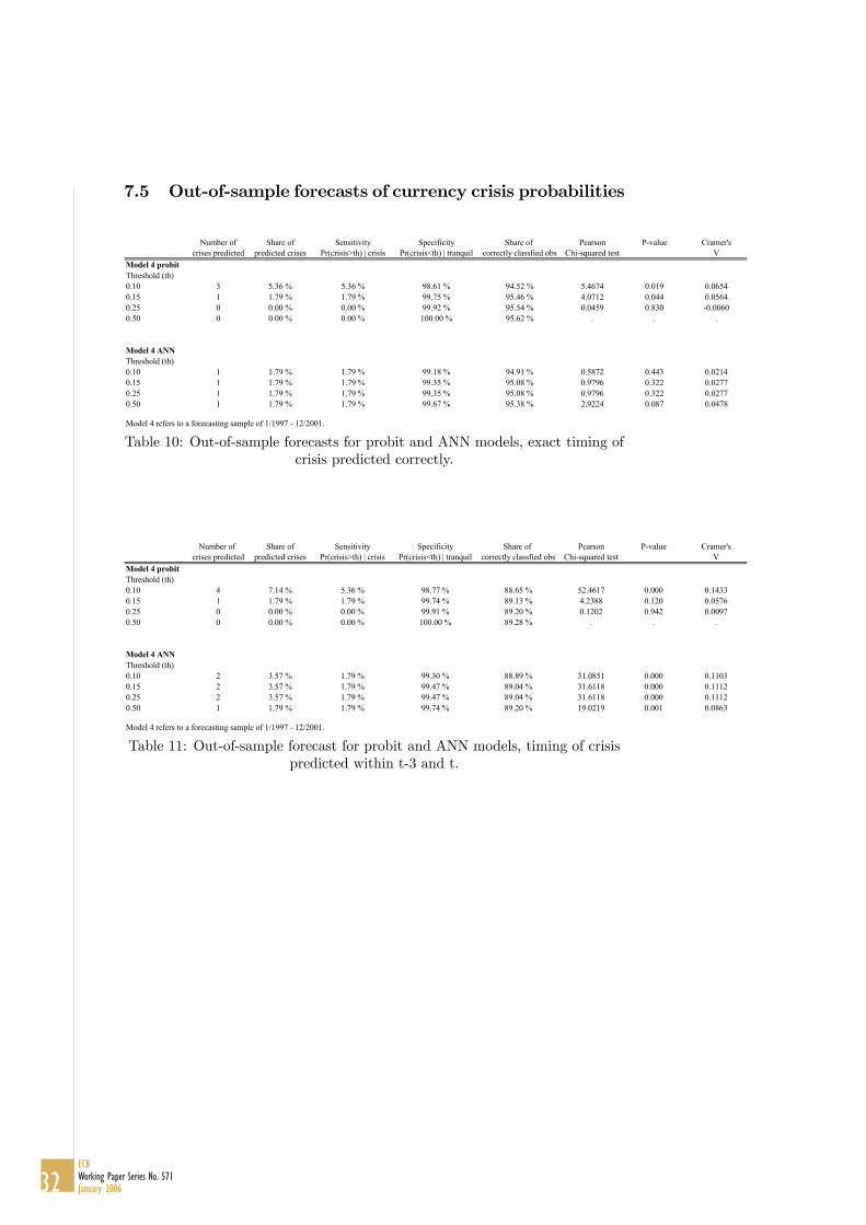
7.5 Out-of-sample forecasts of currency crisis probabilities

Number of Share of Sensitivity Specificity Share of Pearson P-value Cramer'scrises predicted predicted crises Pr(crisis>th) | crisis Pr(crisis<th) | tranquil correctly classfied obs Chi-squared test V

Model 4 probit Threshold (th)0.10 3 5.36 % 5.36 % 98.61 % 94.52 % 5.4674 0.019 0.06540.15 1 1.79 % 1.79 % 99.75 % 95.46 % 4.0712 0.044 0.05640.25 0 0.00 % 0.00 % 99.92 % 95.54 % 0.0459 0.830 -0.00600.50 0 0.00 % 0.00 % 100.00 % 95.62 % . . .

Model 4 ANN Threshold (th)0.10 1 1.79 % 1.79 % 99.18 % 94.91 % 0.5872 0.443 0.02140.15 1 1.79 % 1.79 % 99.35 % 95.08 % 0.9796 0.322 0.02770.25 1 1.79 % 1.79 % 99.35 % 95.08 % 0.9796 0.322 0.02770.50 1 1.79 % 1.79 % 99.67 % 95.38 % 2.9224 0.087 0.0478

Model 4 refers to a forecasting sample of 1/1997 - 12/2001.

Table 10: Out-of-sample forecasts for probit and ANN models, exact timing ofcrisis predicted correctly.

Number of Share of Sensitivity Specificity Share of Pearson P-value Cramer'scrises predicted predicted crises Pr(crisis>th) | crisis Pr(crisis<th) | tranquil correctly classfied obs Chi-squared test V

Model 4 probitThreshold (th)0.10 4 7.14 % 5.36 % 98.77 % 88.65 % 52.4617 0.000 0.14330.15 1 1.79 % 1.79 % 99.74 % 89.13 % 4.2388 0.120 0.05760.25 0 0.00 % 0.00 % 99.91 % 89.20 % 0.1202 0.942 0.00970.50 0 0.00 % 0.00 % 100.00 % 89.28 % . . .

Model 4 ANNThreshold (th)0.10 2 3.57 % 1.79 % 99.30 % 88.89 % 31.0851 0.000 0.11030.15 2 3.57 % 1.79 % 99.47 % 89.04 % 31.6118 0.000 0.11120.25 2 3.57 % 1.79 % 99.47 % 89.04 % 31.6118 0.000 0.11120.50 1 1.79 % 1.79 % 99.74 % 89.20 % 19.0219 0.001 0.0863

Model 4 refers to a forecasting sample of 1/1997 - 12/2001.

Table 11: Out-of-sample forecast for probit and ANN models, timing of crisispredicted within t-3 and t.


7.6 Goodness-of-fit measures

Out-of-sample1 2 3 4

Probit model 12/1980 - 12/2001 12/1980 - 12/1989 1/1990 - 12/2001 1/1997 - 12/2001Mean probability of outcome (crisis) 0.0367 0.0366 0.0372 0.0438Mean probability of forecast 0.0367 0.0367 0.0370 0.0145ROC area 0.7841 0.8758 0.7866 0.6335Brier Quadratic Probability Score 0.0307 0.0239 0.0313 0.0420Sander's modified Quadratic Probability Score 0.0326 0.0300 0.0334 0.0420Spiegelhalter's z-statistic -0.5005 -0.1934 -0.1576 8.9898P-value 0.6916 0.5767 0.5626 0.0000

ANN modelMean probability of outcome (crisis) 0.0367 0.0366 0.0372 0.0438Mean probability of forecast 0.0174 0.0293 0.0363 0.0068ROC area 0.7226 0.8671 0.7115 0.4687Brier Quadratic Probability Score 0.0231 0.0155 0.0243 0.0459Sander's modified Quadratic Probability Score 0.0284 0.0273 0.0287 0.0442Spiegelhalter's z-statistic 55.9788 6.1077 0.5507 33.1186P-value 0.0000 0.0000 0.2909 0.0000

In-sample

Table 12: Goodness-of-fit measures.

33ECB


7.7 Comparison of results

Probit1 ANN1 KLR signal2 BP probit2 BF multin. logit3

Share of observations correctly classified 90.3 % 91.5 % 77.0 % 81.0 % 83.9 %Share of crises correctly classified 22.1 % 45.6 % 41.0 % 44.0 % 73.7 %Share of tranquil periods correctly classified 99.5 % 99.7 % 85.0 % 89.0 % 95.0 %Share of false alarms of total alarms 41.2%+ 26.2%++ 63.0 % 57.0 % 44.1 %

1) Threshold 25%. (Pre)crisis period is correctly classified when the estimated probability of crisis is above the cut-off probability and a crisis ensues within 3 months. Estimation sample: 12/1980 - 12/2001 with 24 countries. + There were a total of 51 alarms of which 21 were incorrect, ++ there were a total of 84 alarms of which 22 were incorrect.2) Source: Berg and Pattillo (1999), page 570 with a threshold 25%. KLR refers to Kaminsky et al. (1998), while BP probit refers to Berg and Patillo (1999). (Pre)crisis period is correctly classified when the estimated probability of crisis is above the cut-off probability and a crisis ensues within 24 months. Estimation sample: 1/1970 - 4/1995 with 23 countries.3) Source: Bussière and Fratzscher (2002), page 25 with a threshold of 20%. (Pre)crisis period is correctly classified when the estimated probability of crisis is above the cut-off probability and a crisis ensues within 12 months. Estimation sample: 12/1993 - 9/2001 with 20 countries.

Table 13: Comparision of in-sample fit to selected earlier papers.

Probit1 ANN1 KLR signal2 BP probit2 KL RE probit3

Share of observations correctly classified 89.2 % 89.0 % 69.0 % 76.0 % 89.2 %Share of crises correctly classified 0.0 % 3.6 % 25.0 % 16.0 % 50.0 %Share of tranquil periods correctly classified 99.9 % 99.5 % 85.0 % 93.0 % 95.2 %Share of false alarms of total alarms 100%* 71.4%** 63.0 % 61.0 % 10.0 %

1) Threshold 25%. (Pre)crisis period is correctly classified when the estimated probability of crisis is above the cut-off probability and a crisis ensues within 3 months. Forecasting sample: 1/1997 - 12/2001 with 24 countries. * There was only 1 alarm, which was incorrect, ** there were 7 signals of which 5 were incorrect.2) Source: Berg and Pattillo (1999), page 576 with a threshold 25%. KLR refers to Kaminsky et al. (1998), while BP probit refers to Berg and Patillo (1999). (Pre)crisis period is correctly classified when the estimated probability of crisis is above the cut-off probability and a crisis ensues within 24 months. Forecasting sample: 5/1995 - 12/1997 with 23 countries.3) Source: Komulainen and Lukkarila (2003), page 259 with a threshold of 25%. (Pre)crisis period is correctly classified when the estimated probability of crisis is above the cut-off probability and a crisis ensues within 12 months. Forecasting sample: 1/1997 - 12/2001 with 31 countries.

Table 14: Comparision of out-of-sample forecasts to selected earlier papers.


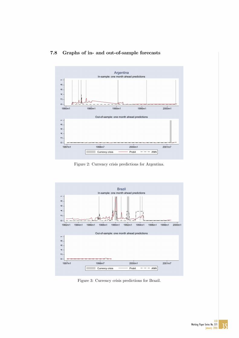
7.8 Graphs of in- and out-of-sample forecasts

0.2

.4.6

.81

1980m1 1985m1 1990m1 1995m1 2000m1

In-sample: one month ahead predictionsArgentina

0.2

.4.6

.81

1997m1 1998m7 2000m1 2001m7

Currency crisis Probit ANN

Out-of-sample: one month ahead predictions

Figure 2: Currency crisis predictions for Argentina.

0.2

.4.6

.81

1982m1 1984m1 1986m1 1988m1 1990m1 1992m1 1994m1 1996m1 1998m1 2000m1

In-sample: one month ahead predictionsBrazil

0.2

.4.6

.81

1997m1 1998m7 2000m1 2001m7



Figure 3: Currency crisis predictions for Brazil.

35ECB


0.2

.4.6

.81

1980m1 1985m1 1990m1 1995m1 2000m1

In-sample: one month ahead predictionsChile

0.2

.4.6

.81

1997m1 1998m7 2000m1 2001m7



Figure 4: Currency crisis predictions for Chile.

0.2

.4.6

.81

1986m1 1988m1 1990m1 1992m1 1994m1 1996m1 1998m1 2000m1 2002m1

In-sample: one month ahead predictionsColombia

0.2

.4.6

.81

1997m1 1998m7 2000m1 2001m7



Figure 5: Currency crisis predictions for Colombia.


0.2

.4.6

.81

1994m1 1996m1 1998m1 2000m1 2002m1

In-sample: one month ahead predictionsCzech Republic

0.2

.4.6

.81

1997m1 1998m7 2000m1 2001m7



Figure 6: Currency crisis predictions for Czech Republic.

0.2

.4.6

.81

1994m1 1996m1 1998m1 2000m1 2002m1

In-sample: one month ahead predictionsEcuador

0.2

.4.6

.81

1997m1 1998m7 2000m1 2001m7



Figure 7: Currency crisis predictions for Ecuador.

37ECB


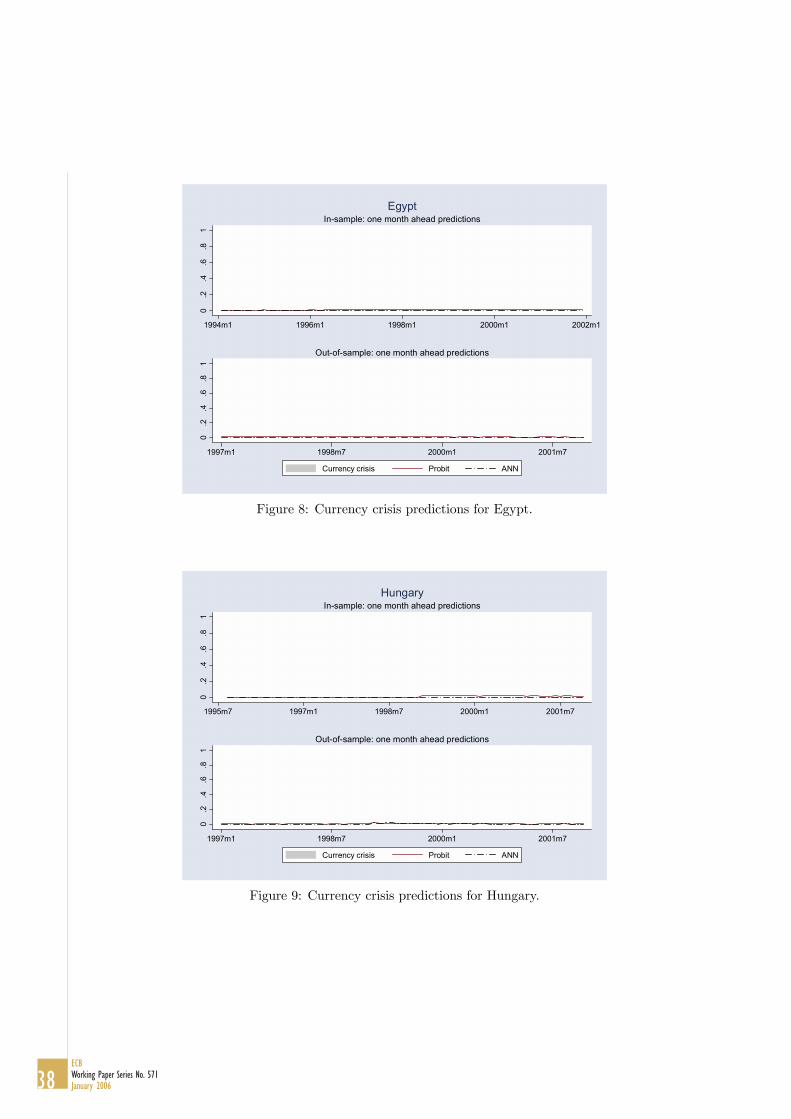
0.2

.4.6

.81

1994m1 1996m1 1998m1 2000m1 2002m1

In-sample: one month ahead predictionsEgypt

0.2

.4.6

.81

1997m1 1998m7 2000m1 2001m7



Figure 8: Currency crisis predictions for Egypt.

0.2

.4.6

.81

1995m7 1997m1 1998m7 2000m1 2001m7

In-sample: one month ahead predictionsHungary

0.2

.4.6

.81

1997m1 1998m7 2000m1 2001m7



Figure 9: Currency crisis predictions for Hungary.


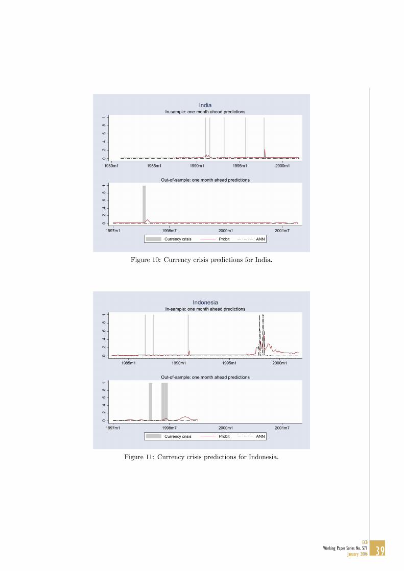
0.2

.4.6

.81

1980m1 1985m1 1990m1 1995m1 2000m1

In-sample: one month ahead predictionsIndia

0.2

.4.6

.81

1997m1 1998m7 2000m1 2001m7



Figure 10: Currency crisis predictions for India.

0.2

.4.6

.81

1985m1 1990m1 1995m1 2000m1

In-sample: one month ahead predictionsIndonesia

0.2

.4.6

.81

1997m1 1998m7 2000m1 2001m7



Figure 11: Currency crisis predictions for Indonesia.

39ECB


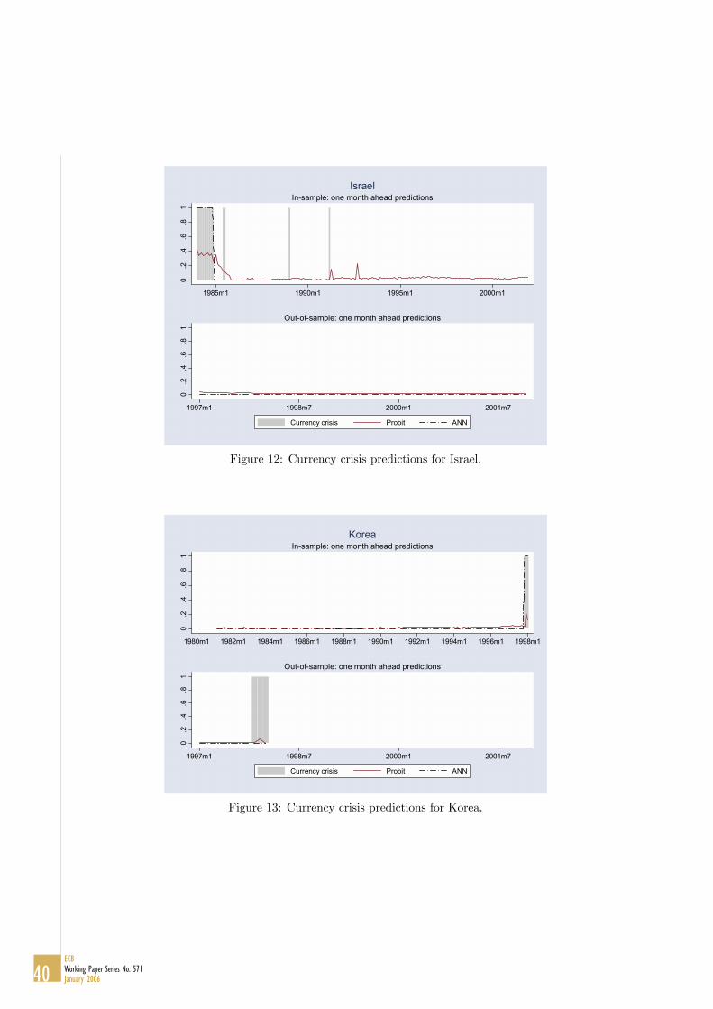
0.2

.4.6

.81

1985m1 1990m1 1995m1 2000m1

In-sample: one month ahead predictionsIsrael

0.2

.4.6

.81

1997m1 1998m7 2000m1 2001m7



Figure 12: Currency crisis predictions for Israel.

0.2

.4.6

.81

1980m1 1982m1 1984m1 1986m1 1988m1 1990m1 1992m1 1994m1 1996m1 1998m1

In-sample: one month ahead predictionsKorea

0.2

.4.6

.81

1997m1 1998m7 2000m1 2001m7



Figure 13: Currency crisis predictions for Korea.


0.2

.4.6

.81

1980m1 1985m1 1990m1 1995m1 2000m1

In-sample: one month ahead predictionsMalaysia

0.2

.4.6

.81

1997m1 1998m7 2000m1 2001m7



Figure 14: Currency crisis predictions for Malaysia.

0.2

.4.6

.81

1997m7 1998m7 1999m7 2000m7 2001m7

In-sample: one month ahead predictionsMexico

0.2

.4.6

.81

1997m1 1998m7 2000m1 2001m7



Figure 15: Currency crisis predictions for Mexico.

41ECB


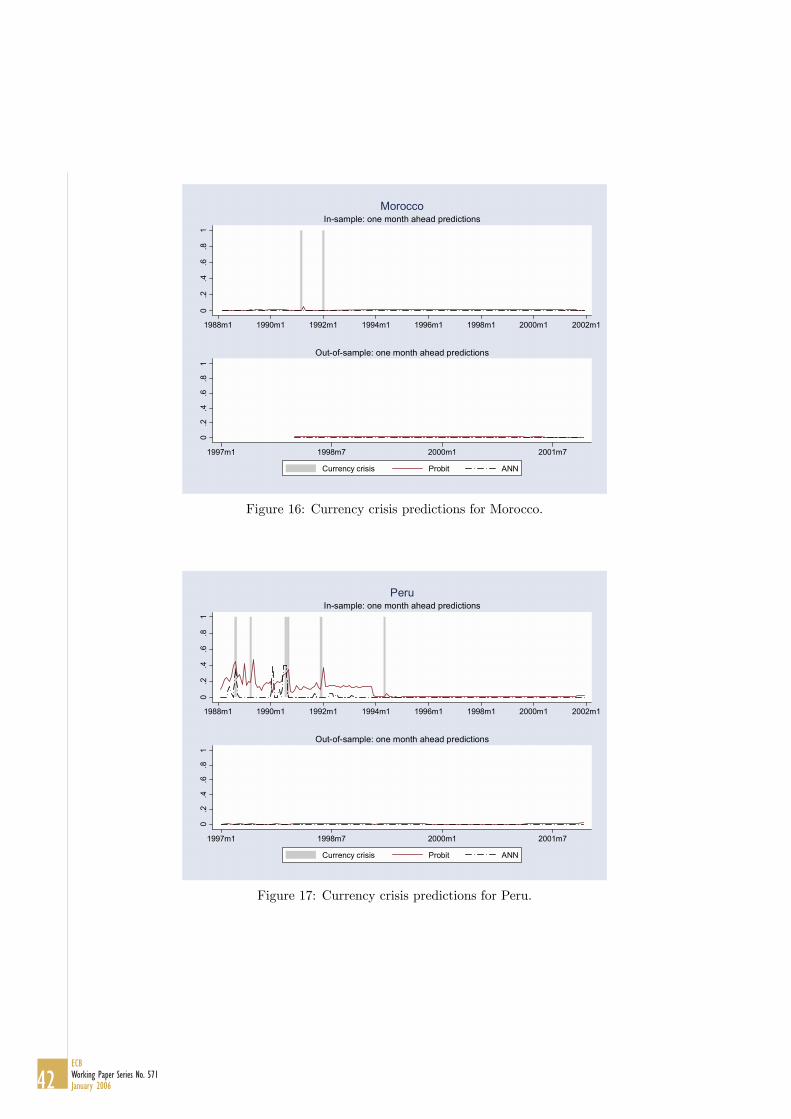
0.2

.4.6

.81

1988m1 1990m1 1992m1 1994m1 1996m1 1998m1 2000m1 2002m1

In-sample: one month ahead predictionsMorocco

0.2

.4.6

.81

1997m1 1998m7 2000m1 2001m7



Figure 16: Currency crisis predictions for Morocco.

0.2

.4.6

.81

1988m1 1990m1 1992m1 1994m1 1996m1 1998m1 2000m1 2002m1

In-sample: one month ahead predictionsPeru

0.2

.4.6

.81

1997m1 1998m7 2000m1 2001m7



Figure 17: Currency crisis predictions for Peru.


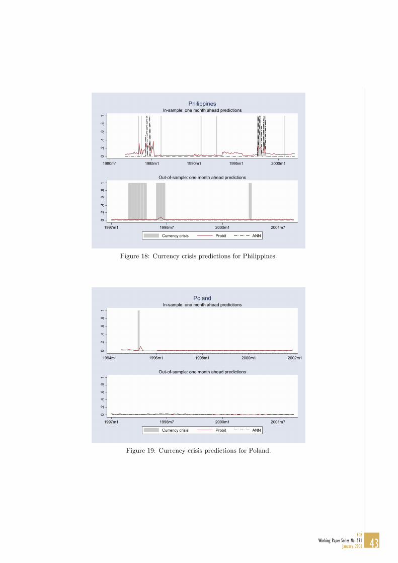
0.2

.4.6

.81

1980m1 1985m1 1990m1 1995m1 2000m1

In-sample: one month ahead predictionsPhilippines

0.2

.4.6

.81

1997m1 1998m7 2000m1 2001m7



Figure 18: Currency crisis predictions for Philippines.

0.2

.4.6

.81

1994m1 1996m1 1998m1 2000m1 2002m1

In-sample: one month ahead predictionsPoland

0.2

.4.6

.81

1997m1 1998m7 2000m1 2001m7



Figure 19: Currency crisis predictions for Poland.

43ECB


0.2

.4.6

.81

1996m1 1998m1 2000m1 2002m1

In-sample: one month ahead predictionsRussia

0.2

.4.6

.81

1997m1 1998m7 2000m1 2001m7



Figure 20: Currency crisis predictions for Russia.

0.2

.4.6

.81

1992m1 1994m1 1996m1 1998m1 2000m1 2002m1

In-sample: one month ahead predictionsSouth Africa

0.2

.4.6

.81

1997m1 1998m7 2000m1 2001m7



Figure 21: Currency crisis predictions for South Africa.


0.2

.4.6

.81

1997m1 1998m7 2000m1 2001m7

In-sample: one month ahead predictionsSlovakia

0.2

.4.6

.81

1997m1 1998m7 2000m1 2001m7



Figure 22: Currency crisis predictions for Slovakia.

0.2

.4.6

.81

1980m1 1985m1 1990m1 1995m1 2000m1

In-sample: one month ahead predictionsThailand

0.2

.4.6

.81

1997m1 1998m7 2000m1 2001m7



Figure 23: Currency crisis predictions for Thailand.

45ECB


0.2

.4.6

.81

1988m1 1990m1 1992m1 1994m1 1996m1 1998m1 2000m1 2002m1

In-sample: one month ahead predictionsTurkey

0.2

.4.6

.81

1997m1 1998m7 2000m1 2001m7



Figure 24: Currency crisis predictions for Turkey.

0.2

.4.6

.81

1985m1 1990m1 1995m1 2000m1

In-sample: one month ahead predictionsVenezuela

0.2

.4.6

.81

1997m1 1998m7 2000m1 2001m7



Figure 25: Currency crisis predictions for Venezuela.


47ECB


For a complete list of Working Papers published by the ECB, please visit the ECB’s website(http://www.ecb.int)

531 “Market power, innovative activity and exchange rate pass-through in the euro area”by S. N. Brissimis and T. S. Kosma, October 2005.

532 “Intra- and extra-euro area import demand for manufactures” by R. Anderton, B. H. Baltagi,F. Skudelny and N. Sousa, October 2005.

533 “Discretionary policy, multiple equilibria, and monetary instruments” by A. Schabert, October 2005.

534 “Time-dependent or state-dependent price setting? Micro-evidence from German metal-workingindustries” by H. Stahl, October 2005.

535 “The pricing behaviour of firms in the euro area: new survey evidence” by S. Fabiani, M. Druant,I. Hernando, C. Kwapil, B. Landau, C. Loupias, F. Martins, T. Y. Mathä, R. Sabbatini, H. Stahl andA. C. J. Stokman, October 2005.

536 “Heterogeneity in consumer price stickiness: a microeconometric investigation” by D. Fougère,H. Le Bihan and P. Sevestre, October 2005.

537 “Global inflation” by M. Ciccarelli and B. Mojon, October 2005.

538 “The price setting behaviour of Spanish firms: evidence from survey data” by L. J. Álvarez andI. Hernando, October 2005.

539 “Inflation persistence and monetary policy design: an overview” by A. T. Levin and R. Moessner,November 2005.

540 “Optimal discretionary policy and uncertainty about inflation persistence” by R. Moessner,November 2005.

541 “Consumer price behaviour in Luxembourg: evidence from micro CPI data” by P. Lünnemannand T. Y. Mathä, November 2005.

542 “Liquidity and real equilibrium interest rates: a framework of analysis” by L. Stracca,November 2005.

543 “Lending booms in the new EU Member States: will euro adoption matter?”by M. Brzoza-Brzezina, November 2005.

544 “Forecasting the yield curve in a data-rich environment: a no-arbitrage factor-augmentedVAR approach” by E. Mönch, November 2005.

545 “Trade integration of Central and Eastern European countries: lessons from a gravity model”by M. Bussière, J. Fidrmuc and B. Schnatz, November 2005.

546 “The natural real interest rate and the output gap in the euro area: a joint estimation”by J. Garnier and B.-R. Wilhelmsen, November 2005.

European Central Bank Working Paper Series


547 “Bank finance versus bond finance: what explains the differences between US and Europe?”by F. de Fiore and H. Uhlig, November 2005.

548 “The link between interest rates and exchange rates: do contractionary depreciations make adifference?” by M. Sánchez, November 2005.

549 “Eigenvalue filtering in VAR models with application to the Czech business cycle”by J. Beneš and D. Vávra, November 2005.

550 “Underwriter competition and gross spreads in the eurobond market” by M. G. Kollo,November 2005.

551 “Technological diversification” by M. Koren and S. Tenreyro, November 2005.

552 “European Union enlargement and equity markets in accession countries”by T. Dvorak and R. Podpiera, November 2005.

553 “Global bond portfolios and EMU” by P. R. Lane, November 2005.

554 “Equilibrium and inefficiency in fixed rate tenders” by C. Ewerhart, N. Cassola and N. Valla,November 2005.

555 “Near-rational exuberance” by J. Bullard, G. W. Evans and S. Honkapohja, November 2005.

556 “The role of real wage rigidity and labor market frictions for unemployment and inflationdynamics” by K. Christoffel and T. Linzert, November 2005.

557 “How should central banks communicate?” by M. Ehrmann and M. Fratzscher, November 2005.

558 “Ricardian fiscal regimes in the European Union” by A. Afonso, November 2005.

559 “When did unsystematic monetary policy have an effect on inflation?” by B. Mojon, December 2005.

560 “The determinants of ‘domestic’ original sin in emerging market economies”by A. Mehl and J. Reynaud, December 2005.

561 “Price setting in German manufacturing: new evidence from new survey data” by H. Stahl,December 2005

562 “The price setting behaviour of Portuguese firms: evidence from survey data” by F. Martins,December 2005

563 “Sticky prices in the euro area: a summary of new micro evidence” by L. J. Álvarez, E. Dhyne,M. M. Hoeberichts, C. Kwapil, H. Le Bihan, P. Lünnemann, F. Martins, R. Sabbatini, H. Stahl,P. Vermeulen and J. Vilmunen, December 2005

564 “Forecasting the central bank’s inflation objective is a good rule of thumb” by M. Diron andB. Mojon, December 2005

565 “The timing of central bank communication” by M. Ehrmann and M. Fratzscher, December 2005

49ECB


566 “Real versus financial frictions to capital investment” by N. Bayraktar, P. Sakellaris andP. Vermeulen, December 2005

567 “Is time ripe for a currency union in emerging East Asia? The role of monetary stabilisation”by M. Sánchez, December 2005

568 “Exploring the international linkages of the euro area: a global VAR analysis” by S. Dées,F. di Mauro, M. H. Pesaran and L. V. Smith, December 2005

569 “Towards European monetary integration: the evolution of currency risk premium as a measurefor monetary convergence prior to the implementation of currency unions” by F. González andS. Launonen, December 2005

570 “Household debt sustainability: what explains household non-performing loans? An empiricalanalysis” by L. Rinaldi and A. Sanchis-Arellano, January 2006

571 “Are emerging market currency crises predictable? A test” by T. A. Peltonen, January 2006

ISSN 1561081-0

9 7 7 1 5 6 1 0 8 1 0 0 5

are emerging market currency crises predictable? a test

Documents