arctic, antarctic, and alpine research, vol. 42, no. 2 ... · area during the 20th century, ... and...
TRANSCRIPT
Twentieth-century Changes in the Thickness and Extent of Arapaho Glacier, FrontRange, Colorado
Benjamin D. Haugen*#
Ted A. Scambos{W. Tad Pfeffer{1 and
Robert S. Anderson*1
*Department of Geological Sciences,
University of Colorado, 399 UCB,
Boulder, Colorado 80309-0399, U.S.A.
{National Snow and Ice Data Center
(NSIDC), University of Colorado, 449
UCB, Boulder, Colorado 80309-0449,
U.S.A.
{Department of Civil, Environmental,
and Architectural Engineering,
University of Colorado, 428 UCB,
Boulder, Colorado 80309-0428, U.S.A.
1Institute of Arctic and Alpine Research
(INSTAAR), University of Colorado,
450 UCB, Boulder, Colorado 80309-
0450, U.S.A.
#Corresponding author: U.S. Army
Engineer Research and Development
Center Geotechnical and Structures
Laboratory (ERDC-GSL), 3909 Halls
Ferry Road, Vicksburg, Mississippi
39180, U.S.A.
Abstract
Changes in Arapaho Glacier, Front Range, Colorado, are determined using
historical maps, aerial photography, and field surveys using ground penetrating
radar (GPR) and Global Positioning System data. Arapaho Glacier lost 52% of its
area during the 20th century, decreasing from 0.34 to 0.16 km2. Between 1900 and
1999 glacial area loss rates increased from an average of 1500 m2 yr21 to
2400 m2 yr21. Average glacial thinning between 1900 and 1960 was 0.76 m yr21, but
slowed to 0.10 m yr21 between 1960 and 2005. Its maximum thickness is
approximately 15 m. If recent trends in area loss continue, Arapaho Glacier may
disappear in as few as 65 years. However, the decline in thinning rate suggests that
the glacier is retreating into a corner of its upper cirque in which increased inputs of
snow from direct precipitation and avalanching, and decreased insolation will greatly
slow its rate of retreat. This may be generally true for many temperate-latitude cirque
glaciers.
DOI: 10.1657/1938-4246-42.2.198
Introduction
Small glaciers in alpine cirques are sensitive indicators of
climate. Worldwide, small glaciers are retreating, and in doing so
are contributing significantly to sea level rise (Lemke et al., 2007;
Meier et al., 2007, 2003). Locally, small glaciers can be significant
sources of water, particularly in late summer for arid temperate
climates, and tracking the decline of these glaciers can provide
important information for water resource planning groups
(Barnett et al., 2005). In the western U.S., small glaciers and ice
fields are generally in rapid decline, but tracking changes in the
rates of decline as the glaciers continue to shrink in area and
recede into sheltered cirques may refine estimates of when seasonal
runoff changes will occur.
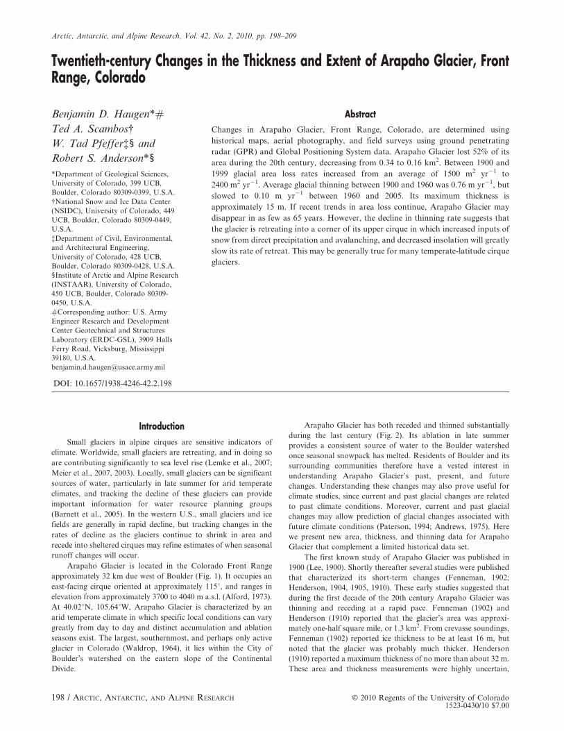
Arapaho Glacier is located in the Colorado Front Range
approximately 32 km due west of Boulder (Fig. 1). It occupies an
east-facing cirque oriented at approximately 115u, and ranges in
elevation from approximately 3700 to 4040 m a.s.l. (Alford, 1973).
At 40.02uN, 105.64uW, Arapaho Glacier is characterized by an
arid temperate climate in which specific local conditions can vary
greatly from day to day and distinct accumulation and ablation
seasons exist. The largest, southernmost, and perhaps only active
glacier in Colorado (Waldrop, 1964), it lies within the City of
Boulder’s watershed on the eastern slope of the Continental
Divide.
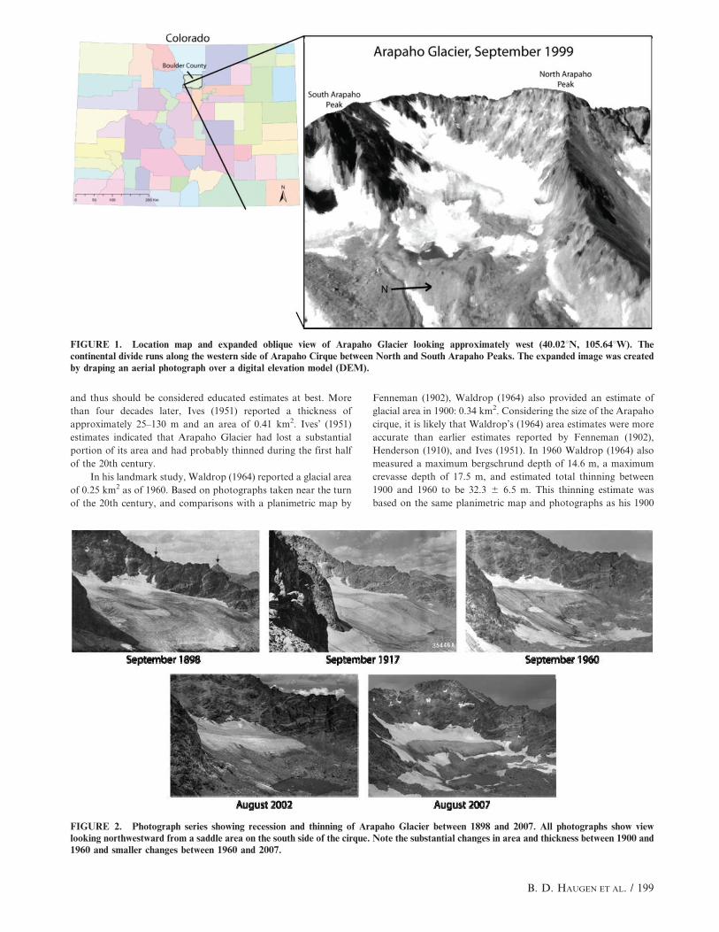
Arapaho Glacier has both receded and thinned substantially
during the last century (Fig. 2). Its ablation in late summer
provides a consistent source of water to the Boulder watershed
once seasonal snowpack has melted. Residents of Boulder and its
surrounding communities therefore have a vested interest in
understanding Arapaho Glacier’s past, present, and future
changes. Understanding these changes may also prove useful for
climate studies, since current and past glacial changes are related
to past climate conditions. Moreover, current and past glacial
changes may allow prediction of glacial changes associated with
future climate conditions (Paterson, 1994; Andrews, 1975). Here
we present new area, thickness, and thinning data for Arapaho
Glacier that complement a limited historical data set.
The first known study of Arapaho Glacier was published in
1900 (Lee, 1900). Shortly thereafter several studies were published
that characterized its short-term changes (Fenneman, 1902;
Henderson, 1904, 1905, 1910). These early studies suggested that
during the first decade of the 20th century Arapaho Glacier was
thinning and receding at a rapid pace. Fenneman (1902) and
Henderson (1910) reported that the glacier’s area was approxi-
mately one-half square mile, or 1.3 km2. From crevasse soundings,
Fenneman (1902) reported ice thickness to be at least 16 m, but
noted that the glacier was probably much thicker. Henderson
(1910) reported a maximum thickness of no more than about 32 m.
These area and thickness measurements were highly uncertain,
Arctic, Antarctic, and Alpine Research, Vol. 42, No. 2, 2010, pp. 198–209
198 / ARCTIC, ANTARCTIC, AND ALPINE RESEARCH E 2010 Regents of the University of Colorado1523-0430/10 $7.00
and thus should be considered educated estimates at best. More
than four decades later, Ives (1951) reported a thickness of
approximately 25–130 m and an area of 0.41 km2. Ives’ (1951)
estimates indicated that Arapaho Glacier had lost a substantial
portion of its area and had probably thinned during the first half
of the 20th century.
In his landmark study, Waldrop (1964) reported a glacial area
of 0.25 km2 as of 1960. Based on photographs taken near the turn
of the 20th century, and comparisons with a planimetric map by
Fenneman (1902), Waldrop (1964) also provided an estimate of
glacial area in 1900: 0.34 km2. Considering the size of the Arapaho
cirque, it is likely that Waldrop’s (1964) area estimates were more
accurate than earlier estimates reported by Fenneman (1902),
Henderson (1910), and Ives (1951). In 1960 Waldrop (1964) also
measured a maximum bergschrund depth of 14.6 m, a maximum
crevasse depth of 17.5 m, and estimated total thinning between
1900 and 1960 to be 32.3 6 6.5 m. This thinning estimate was
based on the same planimetric map and photographs as his 1900
FIGURE 1. Location map and expanded oblique view of Arapaho Glacier looking approximately west (40.02uN, 105.64uW). Thecontinental divide runs along the western side of Arapaho Cirque between North and South Arapaho Peaks. The expanded image was createdby draping an aerial photograph over a digital elevation model (DEM).
FIGURE 2. Photograph series showing recession and thinning of Arapaho Glacier between 1898 and 2007. All photographs show viewlooking northwestward from a saddle area on the south side of the cirque. Note the substantial changes in area and thickness between 1900 and1960 and smaller changes between 1960 and 2007.
B. D. HAUGEN ET AL. / 199
area estimate, complemented with field observations and a plane
table map created from data collected during the summers of 1959
and 1960.
Johnson (1979) reported a maximum bergschrund depth of
greater than 22 m in 1972, a 1973 area of approximately 0.23 km2,
and a minimum thickness of 30–50 m. In an unpublished study,
Pfeffer (2003) calculated thinning between 1960 and 2003 to be
30 m. Using data from nearby Arikaree Glacier, Dyurgerov and
Meier (2005) reconstructed a thinning rate of 0.9 m yr21 between
1960 and 2003. Although it has been the subject of several other
studies (Thornbury, 1928; Outcalt and MacPhail, 1965; Harris,
1968; Alford, 1973; Reheis, 1975; Benedict, 1985), no other
thickness, thinning, or area measurements were found in the
literature. Moreover, the ice thickness and area measurements that
have been reported are highly uncertain. The data reported by
Waldrop (1964) appear to be the best documented, and was thus
drawn on extensively during this study.
In order to constrain the most recent status and changes of
Arapaho Glacier, ice thickness was measured for this study using a
ground penetrating radar (GPR) survey conducted in late October
2007. Glacial area as of September 1999 was measured using a
rectified aerial photograph, and surface elevation profiles were
created from a fall 2005 digital elevation model (DEM). Glacial
area measurements and elevation profiles were compared with
data reported by Waldrop (1964) to produce area loss and
thinning rates during the 20th century. By comparing ice thickness
measurements with calculated area loss and thinning rates, we
have developed an approximate timeline for the recent history and
potential short-term future of Arapaho Glacier. This timeline is of
great significance to both climate researchers and local residents.
In this paper we present the first successful GPR study of Arapaho
Glacier, complemented by a series of new area loss and ice
thinning data. Moreover, this study marks the first accurate
determination of Arapaho Glacier’s thickness, an important
measurement for understanding its past and future changes.
Methods
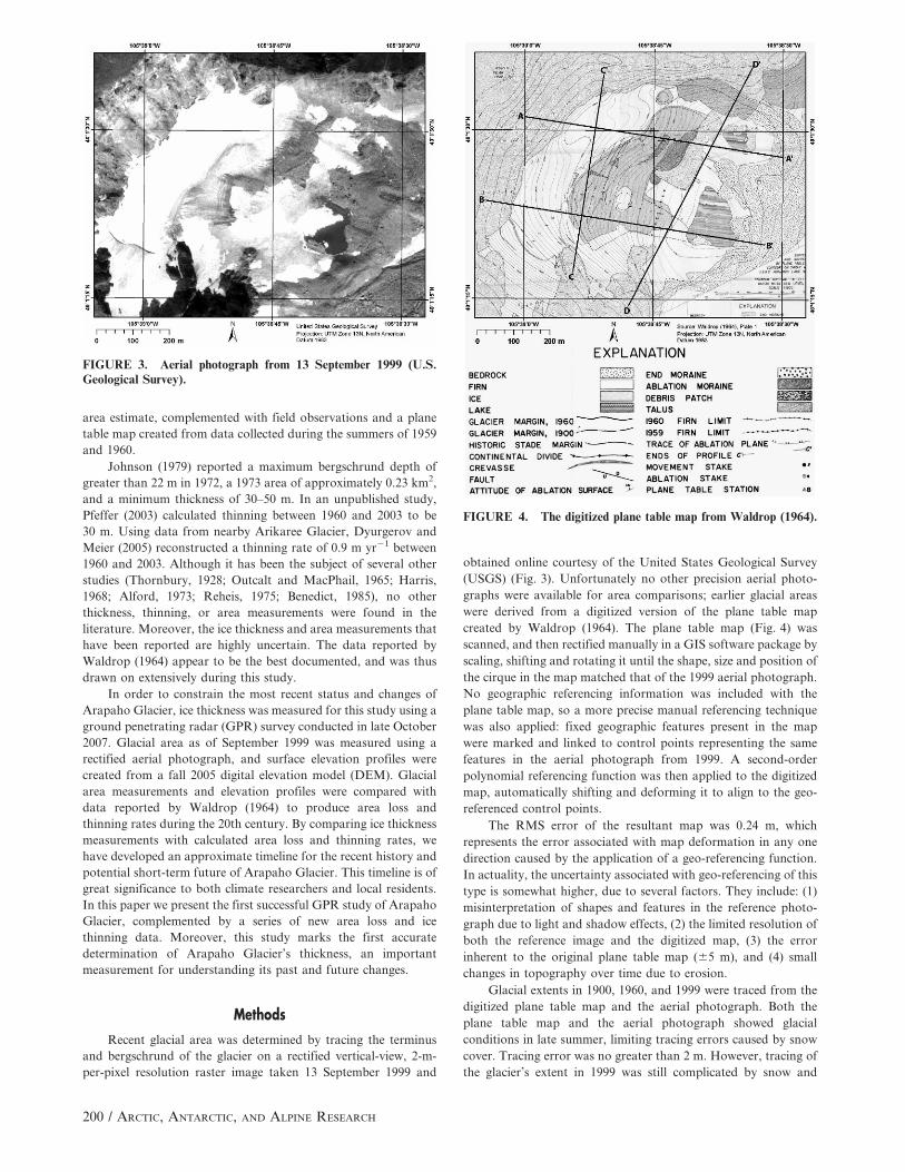
Recent glacial area was determined by tracing the terminus
and bergschrund of the glacier on a rectified vertical-view, 2-m-
per-pixel resolution raster image taken 13 September 1999 and
obtained online courtesy of the United States Geological Survey
(USGS) (Fig. 3). Unfortunately no other precision aerial photo-
graphs were available for area comparisons; earlier glacial areas
were derived from a digitized version of the plane table map
created by Waldrop (1964). The plane table map (Fig. 4) was
scanned, and then rectified manually in a GIS software package by
scaling, shifting and rotating it until the shape, size and position of
the cirque in the map matched that of the 1999 aerial photograph.
No geographic referencing information was included with the
plane table map, so a more precise manual referencing technique
was also applied: fixed geographic features present in the map
were marked and linked to control points representing the same
features in the aerial photograph from 1999. A second-order
polynomial referencing function was then applied to the digitized
map, automatically shifting and deforming it to align to the geo-
referenced control points.
The RMS error of the resultant map was 0.24 m, which
represents the error associated with map deformation in any one
direction caused by the application of a geo-referencing function.
In actuality, the uncertainty associated with geo-referencing of this
type is somewhat higher, due to several factors. They include: (1)
misinterpretation of shapes and features in the reference photo-
graph due to light and shadow effects, (2) the limited resolution of
both the reference image and the digitized map, (3) the error
inherent to the original plane table map (65 m), and (4) small
changes in topography over time due to erosion.
Glacial extents in 1900, 1960, and 1999 were traced from the
digitized plane table map and the aerial photograph. Both the
plane table map and the aerial photograph showed glacial
conditions in late summer, limiting tracing errors caused by snow
cover. Tracing error was no greater than 2 m. However, tracing of
the glacier’s extent in 1999 was still complicated by snow and
FIGURE 3. Aerial photograph from 13 September 1999 (U.S.Geological Survey).
FIGURE 4. The digitized plane table map from Waldrop (1964).
200 / ARCTIC, ANTARCTIC, AND ALPINE RESEARCH
shadows present in the aerial photograph, as well as its limited
resolution. To address this problem, various recent photographs
(Fig. 2) and field observations were used as a guide. The estimated
total uncertainty of the 1999 area measurement is 5%. Polygon
shape files were created from the extent traces and their respective
areas were compared to obtain area change rates for the 1900–
1960 and 1960–1999 periods.
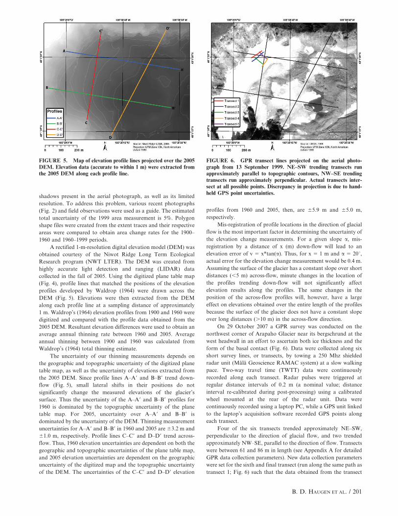
A rectified 1-m-resolution digital elevation model (DEM) was
obtained courtesy of the Niwot Ridge Long Term Ecological
Research program (NWT LTER). The DEM was created from
highly accurate light detection and ranging (LIDAR) data
collected in the fall of 2005. Using the digitized plane table map
(Fig. 4), profile lines that matched the positions of the elevation
profiles developed by Waldrop (1964) were drawn across the
DEM (Fig. 5). Elevations were then extracted from the DEM
along each profile line at a sampling distance of approximately
1 m. Waldrop’s (1964) elevation profiles from 1900 and 1960 were
digitized and compared with the profile data obtained from the
2005 DEM. Resultant elevation differences were used to obtain an
average annual thinning rate between 1960 and 2005. Average
annual thinning between 1900 and 1960 was calculated from
Waldrop’s (1964) total thinning estimate.
The uncertainty of our thinning measurements depends on
the geographic and topographic uncertainty of the digitized plane
table map, as well as the uncertainty of elevations extracted from
the 2005 DEM. Since profile lines A–A9 and B–B9 trend down-
flow (Fig. 5), small lateral shifts in their positions do not
significantly change the measured elevations of the glacier’s
surface. Thus the uncertainty of the A–A9 and B–B9 profiles for
1960 is dominated by the topographic uncertainty of the plane
table map. For 2005, uncertainty over A–A9 and B–B9 is
dominated by the uncertainty of the DEM. Thinning measurement
uncertainties for A–A9 and B–B9 in 1960 and 2005 are 63.2 m and
61.0 m, respectively. Profile lines C–C9 and D–D9 trend across-
flow. Thus, 1960 elevation uncertainties are dependent on both the
geographic and topographic uncertainties of the plane table map,
and 2005 elevation uncertainties are dependent on the geographic
uncertainty of the digitized map and the topographic uncertainty
of the DEM. The uncertainties of the C–C9 and D–D9 elevation
profiles from 1960 and 2005, then, are 65.9 m and 65.0 m,
respectively.
Mis-registration of profile locations in the direction of glacial
flow is the most important factor in determining the uncertainty of
the elevation change measurements. For a given slope a, mis-
registration by a distance of x (m) down-flow will lead to an
elevation error of v 5 x*tan(a). Thus, for x 5 1 m and a 5 20u,actual error for the elevation change measurement would be 0.4 m.
Assuming the surface of the glacier has a constant slope over short
distances (,5 m) across-flow, minute changes in the location of
the profiles trending down-flow will not significantly affect
elevation results along the profiles. The same changes in the
position of the across-flow profiles will, however, have a large
effect on elevations obtained over the entire length of the profiles
because the surface of the glacier does not have a constant slope
over long distances (.10 m) in the across-flow direction.
On 29 October 2007 a GPR survey was conducted on the
northwest corner of Arapaho Glacier near its bergschrund at the
west headwall in an effort to ascertain both ice thickness and the
form of the basal contact (Fig. 6). Data were collected along six
short survey lines, or transects, by towing a 250 Mhz shielded
radar unit (Mala Geoscience RAMAC system) at a slow walking
pace. Two-way travel time (TWTT) data were continuously
recorded along each transect. Radar pulses were triggered at
regular distance intervals of 0.2 m (a nominal value; distance
interval re-calibrated during post-processing) using a calibrated
wheel mounted at the rear of the radar unit. Data were
continuously recorded using a laptop PC, while a GPS unit linked
to the laptop’s acquisition software recorded GPS points along
each transect.
Four of the six transects trended approximately NE–SW,
perpendicular to the direction of glacial flow, and two trended
approximately NW–SE, parallel to the direction of flow. Transects
were between 61 and 86 m in length (see Appendix A for detailed
GPR data collection parameters). New data collection parameters
were set for the sixth and final transect (run along the same path as
transect 1; Fig. 6) such that the data obtained from the transect
FIGURE 5. Map of elevation profile lines projected over the 2005DEM. Elevation data (accurate to within 1 m) were extracted fromthe 2005 DEM along each profile line.
FIGURE 6. GPR transect lines projected on the aerial photo-graph from 13 September 1999. NE–SW trending transects runapproximately parallel to topographic contours, NW–SE trendingtransects run approximately perpendicular. Actual transects inter-sect at all possible points. Discrepancy in projection is due to hand-held GPS point uncertainties.
B. D. HAUGEN ET AL. / 201
line 6 would show reflectors at greater depths than the first five
transects. Other than to confirm that there were no other potential
ice-bedrock-interface reflectors than those identified in transects
1–5, transect 6 was not considered in this study.
Data from the October 2007 expedition were collected using a
directional, shielded system designed to minimize ringing and
reflections from surface features. An earlier attempt to collect
GPR data using a simple 10 MHz radar system in March 2007
produced noisy, convoluted data that revealed no distinct
subsurface reflectors. The poor quality of the data was likely
due to ‘‘ringing’’ of unshielded radar waves between the steep
rocky walls of the tight cirque and the radar antennas. Unshielded
25 MHz profiles acquired in June 2004 also produced similarly
uninterpretable results.
At the time of data acquisition snow depth was measured to
be between 0.8 and 1 m. Air temperature was above freezing, and
the surface of the snow was wet with meltwater. However, the
temperature of the snow-ice interface, measured at several
locations, was between 22.4 and 21.9 uC, indicating a minimum
amount of signal-reducing surface meltwater. There was no
evidence to suggest that abundant water was present within the
subsurface or within the glacier, which otherwise might have
affected the radar results.
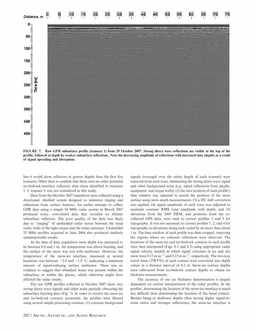
The raw GPR profiles collected in October 2007 show very
strong direct wave signals and other noise partially obscuring the
subsurface layering data (Fig. 7). In order to resolve the snow-ice
and ice-bedrock contacts accurately, the profiles were filtered
using several simple processing routines: (1) constant background
signals (averaged over the entire length of each transect) were
removed from each trace, eliminating the strong direct wave signal
and other background noise (e.g. signal reflections from people,
equipment, and cirque walls); (2) the zero position of each profile’s
time window was adjusted to match the position of the snow
surface using snow depth measurements; (3) a DC shift correction
was applied; (4) signal amplitude of each trace was adjusted to
maintain constant RMS total amplitude with depth; and (5)
elevations from the 2005 DEM, and positions from the co-
collected GPS data, were used to correct profiles 3 and 5 for
topography. It was not necessary to correct profiles 1, 2, and 4 for
topography as elevations along each varied by no more than about
1 m. The time window of each profile was then cropped, removing
the regions where no coherent reflections were observed. The
locations of the snow-ice and ice-bedrock contacts in each profile
were then interpreted (Figs. 8.1 and 8.2) using appropriate radar
signal velocity models in which signal velocities in ice and dry
snow were 0.17 m ns21 and 0.23 m ns21, respectively. The two-way
travel times (TWTTs) of each contact were converted into depth
values at a distance interval of 0.2 m. Snow-ice contact depths
were subtracted from ice-bedrock contact depths to obtain ice
thickness measurements.
The accuracy of our ice thickness determination is largely
dependent on correct interpretation of the radar profiles. In the
profiles, determining the location of the snow-ice interface is much
less difficult than determining the location of the basal contact.
Besides being at shallower depths (thus having higher signal-to-
noise ratios and stronger reflections), the snow-ice interface is
FIGURE 7. Raw GPR subsurface profile (transect 1) from 29 October 2007. Strong direct wave reflections are visible at the top of theprofile, followed at depth by weaker subsurface reflections. Note the decreasing amplitude of reflections with increased time (depth) as a resultof signal spreading and absorption.
202 / ARCTIC, ANTARCTIC, AND ALPINE RESEARCH
relatively smooth, making interpretation of its location more
straightforward. Moreover, snow depth was directly measured at
one location during the radar survey in October 2007, which aided
in interpretation. The basal contact on the other hand, is highly
irregular, and basal reflections are both discontinuous and weak
due to the shielding effect of entrained debris and signal spreading
with depth.
The accuracy of thickness measurements also depends on the
accuracy of the velocity model used to convert TWTTs to depths.
The snow and ice velocities used were not experimentally
determined, and thus are only approximate. However, normal-
move-out analyses of discreet reflectors in each profile show that
the velocities used were accurate to within about 0.01 m*ns21, or
4–6%. This translates to a depth uncertainty of about 61 m. Thus,
accounting for an estimated contact interpretation uncertainty of
60.5 m, the estimated uncertainty of ice thickness measurements
presented here is 61.5 m.
Results
The areas of Arapaho Glacier in 1900 and in 1960, as
measured from the digitized and geo-referenced plane table map,
were 0.34 km2 and 0.25 km2, respectively. These measurements
agree very closely with the values reported by Waldrop (1964)
(Table 1), suggesting that the digitized plane table map was
transformed correctly during geo-referencing. Assuming a con-
stant rate of change, Arapaho Glacier lost approximately 1500 m2
of area each year between 1900 and 1960 (Fig. 9). Under the same
assumption, and if Johnson’s (1979) measurement of glacial area
in 1973 was accurate, then between 1960 and 1973 Arapaho
Glacier decreased in area at an average rate of 1900 m2 yr21, and
between 1973 and 1999 it decreased in area by 2400 m2 yr21. If
Johnson’s (1979) measurement is disregarded, the average annual
loss rate between 1960 and 1999 was 2300 m2 yr21. Given
observed fluctuations in Arapaho Glacier’s mass balance over
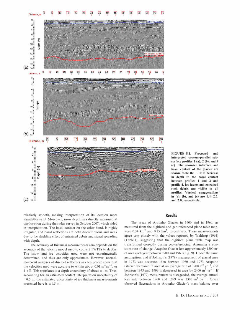
FIGURE 8.1. Processed andinterpreted contour-parallel sub-surface profiles 1 (a), 2 (b), and 4(c). The snow-ice interface andbasal contact of the glacier areshown. Note the ,10 m decreasein depth to the basal contactbetween profiles 1 and 2 andprofile 4. Ice layers and entrainedrock debris are visible in allprofiles. Vertical exaggerationsin (a), (b), and (c) are 1.4, 2.7,and 2.0, respectively.
B. D. HAUGEN ET AL. / 203
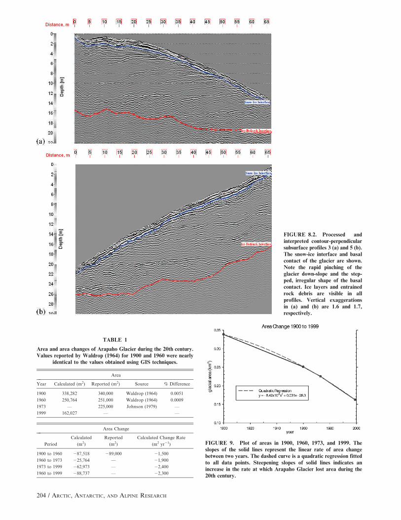
FIGURE 8.2. Processed andinterpreted contour-perpendicularsubsurface profiles 3 (a) and 5 (b).The snow-ice interface and basalcontact of the glacier are shown.Note the rapid pinching of theglacier down-slope and the step-ped, irregular shape of the basalcontact. Ice layers and entrainedrock debris are visible in allprofiles. Vertical exaggerationsin (a) and (b) are 1.6 and 1.7,respectively.
TABLE 1
Area and area changes of Arapaho Glacier during the 20th century.Values reported by Waldrop (1964) for 1900 and 1960 were nearly
identical to the values obtained using GIS techniques.
Area
Year Calculated (m2) Reported (m2) Source % Difference
1900 338,282 340,000 Waldrop (1964) 0.0051
1960 250,764 251,000 Waldrop (1964) 0.0009
1973 — 225,000 Johnson (1979) —
1999 162,027 — —
Area Change
Period
Calculated
(m2)
Reported
(m2)
Calculated Change Rate
(m2 yr21)
1900 to 1960 287,518 289,000 21,500
1960 to 1973 225,764 — 21,900
1973 to 1999 262,973 — 22,400
1960 to 1999 288,737 — 22,300
FIGURE 9. Plot of areas in 1900, 1960, 1973, and 1999. Theslopes of the solid lines represent the linear rate of area changebetween two years. The dashed curve is a quadratic regression fittedto all data points. Steepening slopes of solid lines indicates anincrease in the rate at which Arapaho Glacier lost area during the20th century.
204 / ARCTIC, ANTARCTIC, AND ALPINE RESEARCH
short time scales (Henderson, 1904; Waldrop, 1964; Johnson,
1979), it is highly unlikely that the rate of area change remained
constant from year to year during the time periods analyzed.
Nonetheless, the area change rates obtained here can be used to
draw an important conclusion about the glacier’s behavior during
the 20th century: on average, the rate at which Arapaho Glacier
lost area increased significantly between 1900 and 1999 (Fig. 9).
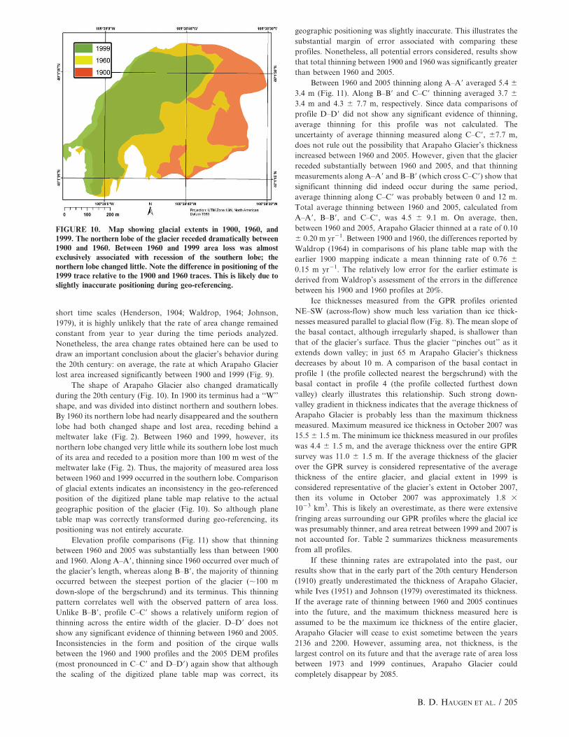
The shape of Arapaho Glacier also changed dramatically
during the 20th century (Fig. 10). In 1900 its terminus had a ‘‘W’’
shape, and was divided into distinct northern and southern lobes.
By 1960 its northern lobe had nearly disappeared and the southern
lobe had both changed shape and lost area, receding behind a
meltwater lake (Fig. 2). Between 1960 and 1999, however, its
northern lobe changed very little while its southern lobe lost much
of its area and receded to a position more than 100 m west of the
meltwater lake (Fig. 2). Thus, the majority of measured area loss
between 1960 and 1999 occurred in the southern lobe. Comparison
of glacial extents indicates an inconsistency in the geo-referenced
position of the digitized plane table map relative to the actual
geographic position of the glacier (Fig. 10). So although plane
table map was correctly transformed during geo-referencing, its
positioning was not entirely accurate.
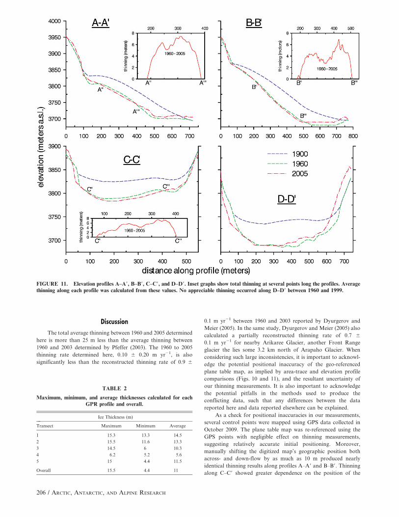
Elevation profile comparisons (Fig. 11) show that thinning
between 1960 and 2005 was substantially less than between 1900
and 1960. Along A–A9, thinning since 1960 occurred over much of
the glacier’s length, whereas along B–B9, the majority of thinning
occurred between the steepest portion of the glacier (,100 m
down-slope of the bergschrund) and its terminus. This thinning
pattern correlates well with the observed pattern of area loss.
Unlike B–B9, profile C–C9 shows a relatively uniform region of
thinning across the entire width of the glacier. D–D9 does not
show any significant evidence of thinning between 1960 and 2005.
Inconsistencies in the form and position of the cirque walls
between the 1960 and 1900 profiles and the 2005 DEM profiles
(most pronounced in C–C9 and D–D9) again show that although
the scaling of the digitized plane table map was correct, its
geographic positioning was slightly inaccurate. This illustrates the
substantial margin of error associated with comparing these
profiles. Nonetheless, all potential errors considered, results show
that total thinning between 1900 and 1960 was significantly greater
than between 1960 and 2005.
Between 1960 and 2005 thinning along A–A9 averaged 5.4 6
3.4 m (Fig. 11). Along B–B9 and C–C9 thinning averaged 3.7 6
3.4 m and 4.3 6 7.7 m, respectively. Since data comparisons of
profile D–D9 did not show any significant evidence of thinning,
average thinning for this profile was not calculated. The
uncertainty of average thinning measured along C–C9, 67.7 m,
does not rule out the possibility that Arapaho Glacier’s thickness
increased between 1960 and 2005. However, given that the glacier
receded substantially between 1960 and 2005, and that thinning
measurements along A–A9 and B–B9 (which cross C–C9) show that
significant thinning did indeed occur during the same period,
average thinning along C–C9 was probably between 0 and 12 m.
Total average thinning between 1960 and 2005, calculated from
A–A9, B–B9, and C–C9, was 4.5 6 9.1 m. On average, then,
between 1960 and 2005, Arapaho Glacier thinned at a rate of 0.10
6 0.20 m yr21. Between 1900 and 1960, the differences reported by
Waldrop (1964) in comparisons of his plane table map with the
earlier 1900 mapping indicate a mean thinning rate of 0.76 6
0.15 m yr21. The relatively low error for the earlier estimate is
derived from Waldrop’s assessment of the errors in the difference
between his 1900 and 1960 profiles at 20%.
Ice thicknesses measured from the GPR profiles oriented
NE–SW (across-flow) show much less variation than ice thick-
nesses measured parallel to glacial flow (Fig. 8). The mean slope of
the basal contact, although irregularly shaped, is shallower than
that of the glacier’s surface. Thus the glacier ‘‘pinches out’’ as it
extends down valley; in just 65 m Arapaho Glacier’s thickness
decreases by about 10 m. A comparison of the basal contact in
profile 1 (the profile collected nearest the bergschrund) with the
basal contact in profile 4 (the profile collected furthest down
valley) clearly illustrates this relationship. Such strong down-
valley gradient in thickness indicates that the average thickness of
Arapaho Glacier is probably less than the maximum thickness
measured. Maximum measured ice thickness in October 2007 was
15.5 6 1.5 m. The minimum ice thickness measured in our profiles
was 4.4 6 1.5 m, and the average thickness over the entire GPR
survey was 11.0 6 1.5 m. If the average thickness of the glacier
over the GPR survey is considered representative of the average
thickness of the entire glacier, and glacial extent in 1999 is
considered representative of the glacier’s extent in October 2007,
then its volume in October 2007 was approximately 1.8 3
1023 km3. This is likely an overestimate, as there were extensive
fringing areas surrounding our GPR profiles where the glacial ice
was presumably thinner, and area retreat between 1999 and 2007 is
not accounted for. Table 2 summarizes thickness measurements
from all profiles.
If these thinning rates are extrapolated into the past, our
results show that in the early part of the 20th century Henderson
(1910) greatly underestimated the thickness of Arapaho Glacier,
while Ives (1951) and Johnson (1979) overestimated its thickness.
If the average rate of thinning between 1960 and 2005 continues
into the future, and the maximum thickness measured here is
assumed to be the maximum ice thickness of the entire glacier,
Arapaho Glacier will cease to exist sometime between the years
2136 and 2200. However, assuming area, not thickness, is the
largest control on its future and that the average rate of area loss
between 1973 and 1999 continues, Arapaho Glacier could
completely disappear by 2085.
FIGURE 10. Map showing glacial extents in 1900, 1960, and1999. The northern lobe of the glacier receded dramatically between1900 and 1960. Between 1960 and 1999 area loss was almostexclusively associated with recession of the southern lobe; thenorthern lobe changed little. Note the difference in positioning of the1999 trace relative to the 1900 and 1960 traces. This is likely due toslightly inaccurate positioning during geo-referencing.
B. D. HAUGEN ET AL. / 205
Discussion
The total average thinning between 1960 and 2005 determined
here is more than 25 m less than the average thinning between
1960 and 2003 determined by Pfeffer (2003). The 1960 to 2005
thinning rate determined here, 0.10 6 0.20 m yr21, is also
significantly less than the reconstructed thinning rate of 0.9 6
0.1 m yr21 between 1960 and 2003 reported by Dyurgerov and
Meier (2005). In the same study, Dyurgerov and Meier (2005) also
calculated a partially reconstructed thinning rate of 0.7 6
0.1 m yr21 for nearby Arikaree Glacier, another Front Range
glacier the lies some 3.2 km north of Arapaho Glacier. When
considering such large inconsistencies, it is important to acknowl-
edge the potential positional inaccuracy of the geo-referenced
plane table map, as implied by area-trace and elevation profile
comparisons (Figs. 10 and 11), and the resultant uncertainty of
our thinning measurements. It is also important to acknowledge
the potential pitfalls in the methods used to produce the
conflicting data, such that any differences between the data
reported here and data reported elsewhere can be explained.
As a check for positional inaccuracies in our measurements,
several control points were mapped using GPS data collected in
October 2009. The plane table map was re-referenced using the
GPS points with negligible effect on thinning measurements,
suggesting relatively accurate initial positioning. Moreover,
manually shifting the digitized map’s geographic position both
across- and down-flow by as much as 10 m produced nearly
identical thinning results along profiles A–A9 and B–B9. Thinning
along C–C9 showed greater dependence on the position of the
FIGURE 11. Elevation profiles A–A9, B–B9, C–C9, and D–D9. Inset graphs show total thinning at several points long the profiles. Averagethinning along each profile was calculated from these values. No appreciable thinning occurred along D–D9 between 1960 and 1999.
TABLE 2
Maximum, minimum, and average thicknesses calculated for eachGPR profile and overall.
Ice Thickness (m)
Transect Maximum Minimum Average
1 15.3 13.3 14.5
2 15.5 11.6 13.3
3 14.5 6 10.3
4 6.2 5.2 5.6
5 15 4.4 11.5
Overall 15.5 4.4 11
206 / ARCTIC, ANTARCTIC, AND ALPINE RESEARCH
profiles obtained from the map, but at no point did any of the
elevation profiles show evidence for thinning outside the range of
uncertainty. Thus we are confident that positional inaccuracies are
not responsible for the discrepancy between our measurements
and the previously reported data.
Pfeffer (2003) based his conclusions on elevation comparisons
along a single profile line. Elevations in 1960 were taken from
Waldrop’s (1964) elevation profile B–B9. Elevations in 2003 were
determined using photogrammetric methods along the same
profile line, making his thinning measurement vulnerable both
to errors in position and the error of the elevation profile from
1960, similarly to our own. However, a careful visual assessment
of the image series in Figure 2 supports our conclusion that the
thinning rate between 1900 and 1960 was significantly greater than
the thinning rate between 1960 and 2005. Pfeffer’s (2003) data
does not reflect this trend. Thus, insofar as the measurements by
Waldrop (1964) are considered accurate (which was a precept of
both this study and Pfeffer’s), we believe that the thinning values
reported here are more accurate than those reported by Pfeffer
(2003).
The average thinning rate between 1960 and 2003 reported by
Dyurgerov and Meier (2005) is a reconstructed value calculated
using a point-degree-day (PDD) ablation model and 5 years of
direct mass balance measurements from Arikaree Glacier (a
nearby Front Range glacier) and Arapaho Glacier. As a first-
order approximation of thinning we believe this method to be an
excellent tool, but maintain our confidence in the thinning rate
reported here for two major reasons. First, as with Pfeffer’s (2003)
results, the photographic record does not support such a
significant rate of thinning. Second, although Arikaree Glacier
and Arapaho Glacier have similar elevations and aspects, and are
located in the same region of the Front Range, these factors alone
are not sufficient to determine a direct correlation between them;
detailed accumulation and incident shortwave solar radiation, or
insolation, data for each would be necessary to determine such a
relationship (Alford, 1973). In the absence of a correlation based
upon these data an accurate picture of Arapaho Glacier’s mass
balance history would be very difficult to reconstruct. Further-
more, even if such a correlation could be established it would
require many years of coherent data to produce an accurate mass
balance reconstruction. Given the inconsistent and variable mass
balance of Arapaho Glacier (Henderson, 1904; Waldrop, 1964;
Johnson, 1979), the five years of data used by Dyurgerov and
Meier (2005) is, in any case, insufficient to produce an accurate
mass balance reconstruction. Similarly, it is no surprise that the
measured thinning rate of Arikaree Glacier was different than that
measured here for Arapaho Glacier; differences in the shape, size
and slope of each glacier’s cirque and the resulting variance of
accumulation and insolation that would thus be expected between
them suggest that Arapaho and Arikaree probably have very
different mass balance histories.
Nonetheless, even if our thinning measurements are consid-
ered low and their maximum uncertainty is applied, average
thinning between 1900 and 1960 was still more than twice the
average thinning measured here for the 1960 to 2005 period. The
photographic record strongly supports this trend. We therefore
maintain that the total thinning of Arapaho Glacier between 1960
and 2005 was significantly less than it was between 1900 and 1960.
The rate at which Arapaho Glacier has been losing area, on
the other hand, has apparently increased over the course of the
20th century. Thus, although it has both thinned and lost a
considerable portion of its area, Arapaho Glacier’s recent changes
have in large part been limited to its extent; its thickness, relative
to its area, has remained somewhat stable in recent decades. Since
localized accumulation and insolation patterns have the greatest
bearing on the mass balance of Front Range glaciers (Alford,
1973), it is crucial that these factors are examined when attempting
to explain Arapaho Glacier’s peculiar pattern of retreat.
Beyond normal snow accumulation, Arapaho Glacier is
sustained by large amounts of snow deposited in its cirque by
wind transport and avalanching (Waldrop, 1964; Outcalt and
MacPhail, 1965). Field observations in March and October of
2007 and October 2009 also suggest, as has been suggested before
(Johnson, 1979), that the majority of secondary snow is deposited
immediately adjacent to the western headwall of the cirque and
directly on top of the thickest portion of the glacier. Also observed
in 2007 was the shortened period of each day that the same region
is exposed to direct sunlight. Thus the region of Arapaho Glacier
that still exists occupies the basin of the cirque adjacent to the
western headwall because it is this region that receives both the
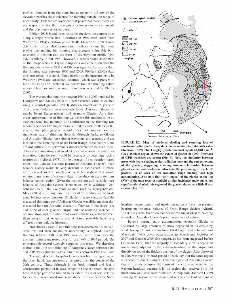
most snow and least solar radiation. A map from Johnson (1979)
showing the region of the cirque that receives the least amount of
FIGURE 12. Map of modeled shading and resulting loss ofshortwave radiation for Arapaho Glacier relative to flat-Earth value(Johnson, 1979). One Langley (insolation unit) equals 41,840 J m22.Gray overlain region shows the extent of glacier in 1999. Positionsof GPR transects are shown (Fig. 6). Note the similarity betweenareas with heavy shading (solar radiation loss) and the current extentof the glacier, suggesting a strong inverse relationship betweenglacial extent and insolation. Also note the positioning of the GPRprofiles—in an area of low insolation (high shading) and highaccumulation. Also note that the ‘‘tongue’’ of the glacier at the top(SW) of the map receives sunlight at high incidence angle and is notsignificantly shaded; this region of the glacier shows very little if anychange (Fig. 10).
B. D. HAUGEN ET AL. / 207
insolation very closely matches the extent of the glacier in 1999
(Fig. 12). This insolation-accumulation pattern supports the
suggestion that the maximum ice thickness measured is likely the
maximum thickness of the entire glacier, since the GPR survey was
conducted in the region of very low insolation and highest
accumulation.
The importance of the high-accumulation zone in the modern
mass balance of Arapaho Glacier may also be seen in the down-
flow profiles (Fig. 8.2). Truncation of layering by the ice surface
indicates intense ablation as distance increases from the headwall.
However, at the very top of the glacier the layering and surface are
nearly parallel, indicating some net accumulation and therefore
some sustaining annual snow mass within 15–20 m of the
uppermost part of the profiles. Note that the near-parallel
relationship of reflectors within the glacier (with the exception of
the lowest layer, where entrained debris may be scattering much of
the return radar signal) implies that no earlier period of intense
ablation is recorded within the remaining ice. In sum, the glacier is
maintained predominantly by local mass balance, redistribution
by flow is negligible, and radar profiles show that the accumu-
lation area is extremely narrow: immediately adjacent the western
headwall (the avalanche and wind-drift zone).
Although more detailed investigations of snow accumulation
and insolation are required to clearly define such a relationship,
heavy accumulation and a lack of exposure to solar radiation over
a limited region of Arapaho Glacier may be enabling sustained ice
thickness while simultaneously allowing for rapid area loss, thus
explaining the unique pattern of retreat reported here.
Presumably, if climate remains stable, there will come a time
when snow accumulation balances insolation-driven ablation. At
such time both the thickness and area of Arapaho Glacier may
reach steady state or require much higher rates of climate warming
to alter. This possibility suggests that the survival estimate we
discuss for Arapaho Glacier may be an underestimate; it is
possible that Arapaho Glacier will continue to exist in some form
for many decades to come. Judging from recent photographic
comparisons (Fig. 2) and the marked decrease in thinning rate
between 1960 and 2005, we believe that the rate at which Arapaho
Glacier is losing area is also now slowing, indicating that it may
already be on its way to a smaller but sustained existence.
However, it is unlikely that the climate will remain stable.
Increased greenhouse gases in the atmosphere are forcing a
warmer climate. As a result, overall accumulation on Arapaho
Glacier will likely drop as some precipitation that once fell as snow
begins to fall as rain, and as the length of the annual melt season
increases. Warming that began in the mid to late 19th century
initiated the glacier’s retreat, and as warming continues its retreat
will likely also continue. So although it may be able to retreat into
a region of the cirque where it is stable, it is also possible that
continued climate forcing will destabilize the glacier enough to
cause its complete disappearance.
Conclusion
Although limited by the availability, accuracy, and integra-
tion of past data, this study illustrates important past trends and
current aspects of Arapaho Glacier. Over the course of the 20th
century, Arapaho Glacier has shown a pattern of increasingly
rapid area loss and decreasingly rapid thinning. Its average
maximum thickness, inferred from the region of the glacier where
GPR data were collected, is 15.5 m. It covers an area of 0.16 km2
and its volume is approximately 1.8 3 1023 km3. If past trends
continue, Arapaho Glacier could cease to exist in as few as
65 years. Observed 20th century trends may or may not continue,
but augmenting the data presented here with repeated GPR
analysis and future studies of accumulation and insolation
patterns, and thickness and area measurements, will help to
constrain the future of Arapaho Glacier as well as provide a
valuable data set for climatological studies.
Acknowledgments
The authors would like to thank the many contributors to thisstudy from the National Snow and Ice Data Center (NSIDC) andthe Institute of Arctic and Alpine Research (INSTAAR) at theUniversity of Colorado at Boulder: Rob Bauer, Terry Haran,Chandler Engel, Andy Mahoney, Peter Gibbons, StephanieRenfrow, David Fanning, and Molly McAllister. B. D. Haugenwould like to extend special thanks to Rob Roscow and WinstonVoigt for their labor and assistance, as well as to Jason Neff at theUniversity of Colorado Department of Geological Sciences andAlan Townsend at INSTAAR for their review of an early versionof this manuscript. This study was supported in part by theUndergraduate Research Opportunities Program (UROP) at theUniversity of Colorado at Boulder. The authors acknowledge theaid of the National Center for Airborne Laser Mapping forgeneration of the high quality 2005 DEM. R. S. Andersonacknowledges support from the Boulder Creek Critical ZoneObservatory (BcCZO).
References Cited
Alford, D. L., 1973: Cirque glaciers of the Colorado Front Range:mesoscale aspects of a glacier environment. PhD thesis.Department of Geography, University of Colorado at Boulder.
Andrews, J. T., 1975: Glacial Systems, an Approach to Glaciers andTheir Environments. Environmental Systems Series. NorthScituate, Massachusetts: Duxbury Press.
Barnett, T. P., Adam, J. C., and Lettenmaier, D. P., 2005:Potential impacts of a warming climate on water availability insnow-dominated regions. Nature, 438: doi:10.1038/nature04141.
Benedict, J. B., 1985: Arapaho Pass; glacial geology and archeo-logy at the crest of the Colorado Front Range. Ward, Colo-rado: Center for Mountain Archeology, Research ReportNo. 3.
Dyurgerov, M. B., and Meier, M. F., 2005: Glaciers and thechanging Earth system: a 2004 snapshot. Boulder, Colorado:Institute of Arctic, Antarctic and Alpine Research, University ofColorado, Occasional Paper No. 58.
Fenneman, N. M., 1902: The Arapahoe Glacier in 1902. Journal ofGeology, 10: 839–851.
Harris, S. A., 1968: Till fabrics and speed of movement of theArapahoe Glacier, Colorado. The Professional Geographer,20(3): 195–198.
Henderson, J., 1904: Arapahoe Glacier in 1903. Journal ofGeology, 12: 30–33.
Henderson, J., 1905: Arapahoe Glacier in 1905. Journal ofGeology, 13: 556.
Henderson, J., 1910: Extinct and existing glaciers of Colorado.University of Colorado Studies, 8(1): 33–76.
Ives, R. L., 1951: Modern glaciers of the Arapaho massif,Colorado. The Scientific Monthly, 13: 25–36.
Johnson, J. B., 1979: Mass balance and aspects of the glacierenvironment, Front Range, Colorado, 1969–1973. PhD thesis.Department of Geological Sciences, University of Colorado atBoulder.
Lee, W. T., 1900: The glacier of Mt. Arapahoe, Colorado. Journalof Geology, 8: 647–654.
Lemke, P., Ren, J., Alley, R. B., Allison, I., Carrasco, J., Flato, G.,Fujii, Y., Kaser, G., Mote, P., Thomas, R. H., and Zhang, T.,2007: Observations: changes in snow, ice and frozen ground. In
208 / ARCTIC, ANTARCTIC, AND ALPINE RESEARCH
Solomon, S. (ed.), Climate change 2007: the physical sciencebasis; summary for policymakers, technical summary andfrequently asked questions. Part of the Working Group Icontribution to the Fourth Assessment Report of the Intergovern-mental Panel on Climate Change. Nairobi: published for theIntergovernmental Panel on Climate Change by UNEP,337–383.
Meier, M. F., Dyurgerov, M. B., and McCabe, G. J., 2003: Thehealth of glaciers: recent changes in glacier regime. ClimaticChange, 59(1–2): 123–125, doi: 10.1023/A:1024410528427.
Meier, M. F., Dyurgerov, M. B., Rick, U. R., O’Neel, S.,Pfeffer, W. T., Anderson, R. S., Anderson, S. P., andGlaznovsky, A. F., 2007: Small glaciers dominate eustatic sea-level rise in the 21st century. Science, 317(5841): 1064–1067.
Outcalt, S. I., and MacPhail, D. D., 1965: A survey ofneoglaciation in the Front Range of Colorado. University ofColorado Studies Series in Earth Sciences, 4.
Paterson, W. S. B., 1994: The Physics of Glaciers. Third edition.Tarrytown, New York: Elsevier Science Inc.
Pfeffer, W. T., 2003: Unpublished photogrammetric survey.Contact: [email protected].
Reheis, M. J., 1975: Source, transportation and deposition ofdebris on Arapaho Glacier, Front Range, Colorado, U.S.A.Journal of Glaciology, 14: 407–420.
Thornbury, W. D., 1928: Glaciation on the east side of theColorado Front Range between James Peak and Longs Peak.MS thesis. Department of Geological Sciences, University ofColorado at Boulder.
Waldrop, H. A., 1964: Arapaho Glacier; a sixty-year record.University of Colorado Studies Series in Geology, 3.
MS accepted January 2010
Appendix A
GPR unit: MALA Geoscience RAMACTM 250 MHz shielded
system. Data acquisition software: RAMACTM GroundVisionTM,
MALA Geoscience. Data processing software: RadExplorerTM,
DECO Geophysical
GPR Collection Parameters, 29 October 2007
Transects 1–5
Samples 1042
Sampling Frequency 1658 s21
Signal/Trace distance interval 0.20 m
Antenna frequency 250 MHz
Antenna separation 0.36 m
Time window 628 ns
Stacks 32
Transect 6
Samples 2002
Sampling Frequency 1658 s21
Signal/Trace distance interval 0.30 m
Antenna frequency 250 MHz
Antenna separation 0.36 m
Time window 1207 ns
Stacks 32
Transect Dimensions
Transect Length # Traces
1 75.97 377
2 85.44 424
3 66.7 331
4 61.46 305
5 66.5 330
6 55.87 186
B. D. HAUGEN ET AL. / 209