architectural layout design optimization fileeng. opt., 2002, vol. 34(5), pp. 461–484...

Eng. Opt., 2002, Vol. 34(5), pp. 461–484

ARCHITECTURAL LAYOUT DESIGN OPTIMIZATION

JEREMY J. MICHALEKa,*, RUCHI CHOUDHARYb and PANOS Y. PAPALAMBROSa

aOptimal Design Laboratory, Department of Mechanical Engineering, University of Michigan,Ann Arbor, Michigan 48109-2125, USA; bCollege of Architecture and Urban Planning,

University of Michigan, Ann Arbor, Michigan 48109-2125, USA

(Received 28 August 2001; In final form 26 February 2002)

This article presents an optimization model of the quantifiable aspects of architectural floorplan layout design, and acompanion article presents a method for integrating mathematical optimization and subjective decision makingduring conceptual design. The model presented here offers a new approach to floorplan layout optimization thattakes advantage of the efficiency of gradient-based algorithms, where appropriate, and uses evolutionaryalgorithms to make discrete decisions and do global search. Automated optimization results are comparable toother methods in this research area, and the new formulation makes it possible to integrate the power of humandecision-making into the process.

Keywords: Optimization; Architectural design; Floorplan; Layout

1 INTRODUCTION

Spatial configuration is concerned with finding feasible locations and dimensions for a set of

interrelated objects that meet all design requirements and maximize design quality in terms

of design preferences. Spatial configuration is relevant to all physical design problems, so it

is an important area of inquiry. Research on automation of spatial configuration includes

component packing [11–13], route path planning [18], process and facilities layout, VLSI

design ½16; 17�, and architectural layout [3–10]. Architectural layout is particularly interesting

because in addition to common engineering objectives such as cost and performance, archi-

tectural design is especially concerned with aesthetic and usability qualities of a layout,

which are generally more difficult to describe formally. Also, the components in a building

layout (rooms or walls) often do not have pre-defined dimensions, so every component of the

layout is resizable.

Reported attempts to automate the process of layout design started over 35 years ago [3].

Researchers have used several problem representations and solution search techniques to

describe and solve the problem.

One approach to spatial allocation is to define the available space as a set of grid

squares and use an algorithm to allocate each square to a particular room or activity [4–7]

(see Fig. 1). This problem is inherently discrete and multi-modal. Because of the

* Corresponding author. E-mail: [email protected]

ISSN 0305-215X print; ISSN 1029-0273 online # 2002 Taylor & Francis LtdDOI: 10.1080=0305215021000033735

combinatorial complexity, it cannot be solved exhaustively for reasonably-sized layout pro-

blems. Several heuristic strategies have been developed to find solutions without searching

the design space exhaustively. Liggett and Mitchell [4] use a constructive placement strategy

followed by an iterative improvement strategy. In this method, space is allocated for rooms

one at a time based on the best probable design move at each step. Other researchers have

used stochastic algorithms for search [5–7].

Another approach to representing the building layout design space is to decompose

the problem into two parts: topology and geometry. Topology refers to logical relationships

between layout components. Geometry refers to the position and size of each component

in the layout. Topological decisions define constraints for the geometric design space. For

example, a topological decision that ‘‘room i is adjacent to the north wall of room j’’ restricts

the geometric coordinates of room i relative to room j. Researchers have developed decision-

tree-based combinatorial representations and used constraint satisfaction programming

techniques to enumerate solutions without exhaustive search. Baykan and Fox [8] and

Schwarz, Berry, and Saviv [9] developed variations of this model and have been able to enu-

merate solutions for a studio apartment and for a nine-room building respectively. Medjeoub

and Yannou [10] developed a similar model, but they use a technique of first enumerating all

topologies that can produce at least one feasible geometry. The designer is then able to review

the feasible topological possibilities and select those which s=he wants to explore geometri-

cally. This technique reduces computation dramatically, and they have shown success for up

to twenty rooms.

Successful generation of global quality solutions has been achieved for medium-sized

problems; however, there is still a need for a strategy that can handle larger problems

computationally. It would be useful to take advantage of the speed of gradient-based

algorithms on the geometric aspects of the layout, because they involve continuous variables.

This article develops a mathematical model for the geometric decisions in the layout pro-

blem that allows efficient solution with gradient-based and hybrid local–global methods. This

model is then embedded into another model used for topology decisions that is solved with

heuristic global methods. The geometric optimization process allows fast solution of large

complex problems that also enables a true interactive design process described in a sequel

article [2]. The topology optimization component has had limited success due to the

combinatorial nature of the topology decisions. The interactive optimization tool can be

downloaded from http:==ode.engin.umich.edu.

FIGURE 1 Sample fixed grid allocation layout.

462 J. J. MICHALEK et al.

2 OPTIMIZATION OF GEOMETRY

The geometric optimization problem is posed as a process of finding the best location and

size of a group of interrelated rectangular units. A new decision model is formulated

where all objectives and constraints are continuous functions, and all design variables

have continuous domains.

A Unit is defined as a rectangular, orthogonal space allocated for a specific architectural

function. Examples of architectural functions include living spaces, storage spaces, facilities,

and accessibility spaces. For simplicity, this representation assumes that all Units can be

represented as rectangles or combinations of orthogonal rectangles. This simple representation

can model a large array of architectural layouts, and more complex shapes could be added to

the model to expand this array. Figure 2 shows a Unit represented as a point in space ðx; yÞ, and

the perpendicular distance from that point to each of the four walls: fN ; S;E; and W g. This

model has more variables than necessary to describe the shape; however, it allows an optimiza-

tion algorithm to change the position of a Unit independently without affecting its size (by

changing x or y), and it can change any of the four wall positions independently (by changing

N ; S;E, or W ). Although this model increases the problem dimensionality, it offers a lot of

flexibility to make the best design moves at each step of the optimization.

Units are grouped into several categories based on their function: Rooms, Boundaries,

Hallways, and Accessways. Rooms are Units used for sustained living activity as determined

by the designer. The differentiation between living space vs. non-living space is important

only in optimization objectives that maximize the amount of space used for living relative

to all other space. A Boundary is a Unit that has other Units constrained inside of it, and

it is not considered living space. A Hallway is a Unit with no physical walls that is not a

living space. Hallways function as pathways. An Accessway is a Hallway that is constrained

to geometrically intersect two Units. Accessways are generally restricted to be small,

and they are forced to intersect two other Units. They function to keep the two Units adjacent

and connected, and to ensure that there is room for a door or opening between the rooms.

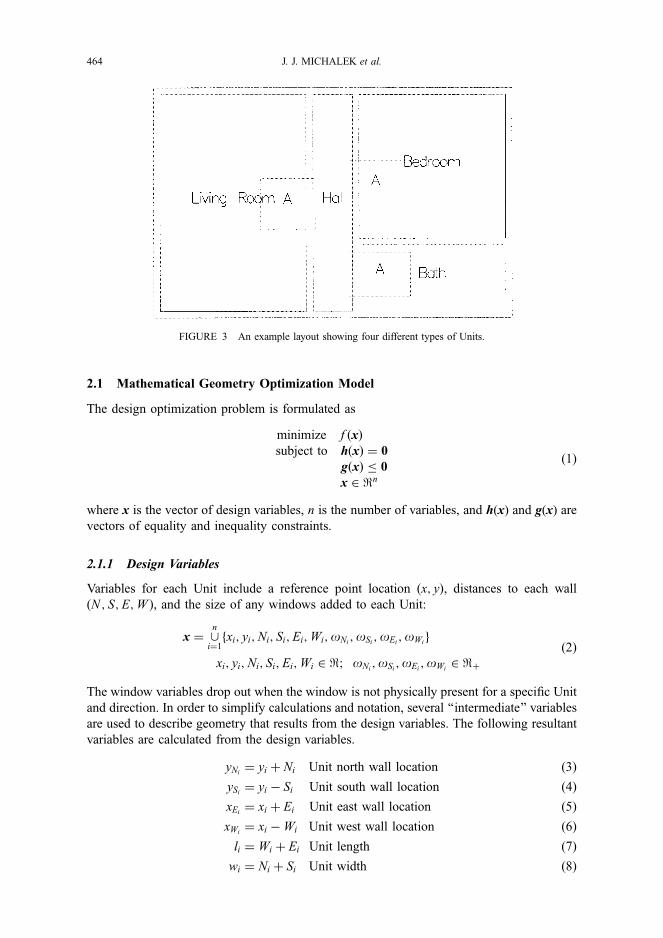
In Figure 3, the external rectangle represents the building Boundary, the living room, bed-

room, and bathroom are Rooms, the hall is a Hallway, and the three Units labeled ‘‘A’’ are

Accessways that define space for a doorway between Units.

Units that are along external walls may also have windows for natural lighting. Window

height can be fixed for each Unit, and window width is a variable. oN ;oS;oE;oW represent

the width of the north, south, east and west windows, respectively.

FIGURE 2 Representation of a Unit.

ARCHITECTURAL DESIGN 463

2.1 Mathematical Geometry Optimization Model

The design optimization problem is formulated as

minimize f ðxÞ

subject to hðxÞ ¼ 0

gðxÞ � 0

x 2 <n

ð1Þ

where x is the vector of design variables, n is the number of variables, and h(x) and g(x) are

vectors of equality and inequality constraints.

2.1.1 Design Variables

Variables for each Unit include a reference point location ðx; yÞ, distances to each wall

ðN ; S;E;W Þ, and the size of any windows added to each Unit:

x ¼ [n

i¼1fxi; yi;Ni; Si;Ei;Wi;oNi

;oSi ;oEi;oWi

g

xi; yi;Ni; Si;Ei;Wi 2 <; oNi;oSi ;oEi

;oWi2 <þ

ð2Þ

The window variables drop out when the window is not physically present for a specific Unit

and direction. In order to simplify calculations and notation, several ‘‘intermediate’’ variables

are used to describe geometry that results from the design variables. The following resultant

variables are calculated from the design variables.

yNi¼ yi þ Ni Unit north wall location ð3Þ

ySi ¼ yi � Si Unit south wall location ð4Þ

xEi¼ xi þ Ei Unit east wall location ð5Þ

xWi¼ xi �Wi Unit west wall location ð6Þ

li ¼ Wi þ Ei Unit length ð7Þ

wi ¼ Ni þ Si Unit width ð8Þ

FIGURE 3 An example layout showing four different types of Units.


These relations are linear, so linear functions of these intermediate variables are also linear

functions of the original variables.

2.1.2 Geometric Design Constraints

The following constraint groups form a toolbox of constraints that can be applied where

appropriate for a particular layout problem. Using the software described in the companion

paper [2], default constraints are automatically added to the model whenever the designer

adds a room, window, etc. The designer can also add, delete, or modify constraints individually.

The Force Inside Constraint Group forces Units into the main building Boundary or other

grouping Boundaries. In order to force Unit i inside Unit j, the following four constraints

must all be satisfied:

yNi� yNj

; ySj � ySi ; xEi� xEj

; and xWj� xWi

ð9Þ

The Prohibit Intersection Constraint functions to prevent two Units from occupying the

same space. By default, one Prohibit Intersection Constraint is added for each combination

of Rooms, Hallways, and Accessways, except where two Units are forced to intersect, or

where one Unit is forced inside of another. In order to prevent Unit i from intersecting

Unit j, at least one of the following constraints must be satisfied

ðxWi� xEj

Þ OR ðxWj� xEi

Þ OR ðySi � yNjÞ OR ðySj � yNi

Þ ð10Þ

The logical disjunction can be represented in negative null form using a min function

minðxEj� xWi

; xEi� xWj

; yNj� ySi ; yNi

� ySj Þ � 0 ð11Þ

This nonlinear, non-smooth formulation is undesirable for gradient-based calculations;

however, the nature of the constraint makes it unavoidable. With this formulation, the con-

straint function acts as a smooth linear function except when the close corners of two

Units are nearly diagonal.

The Force Intersection Constraint Group is used when Units are forced to intersect in

order to ensure access (as Accessways do), or to make a more complex geometric shape

by combining rectangular Units. Forcing intersection is the opposite of prohibiting intersec-

tion, so forcing intersection can be written as the conjunction of the following constraints

ySi � yNj; ySj � yNi

; xWi� xEj

; and xWj� xEi

ð12Þ

Although these constraints ensure intersection of the two Units, they permit intersection at a

point. Designers of architectural spaces are generally interested in intersection that provides

enough room for a doorway or opening. To model this, an additional constraint is included to

enforce overlap in one of the Cartesian directions that is at least as large as the doorway or

opening. Therefore, in addition to intersection, at least one of the following conditions must

be satisfied

yNj� ySi � maxðdi; djÞ Unit i overlaps north wall of Unit j; ð13Þ

yNi� ySj � maxðdi; djÞ Unit i overlaps south wall of Unit j; ð14Þ

xEj� xWi

� maxðdi; djÞ Unit i overlaps east wall of Unit j; ð15Þ

xEi� xWj

� maxðdi; djÞ Unit i overlaps west wall of Unit j: ð16Þ


where di is the minimum size for a door or opening in Unit i. This disjunctive set of

constraints can be represented in negative null form using a min function similar to Eq. (11).

minfmaxðdi; djÞ � xEjþ xWi

; maxðdi; djÞ � xEiþ xWj

;

maxðdi; djÞ � yNjþ ySi ; maxðdi; djÞ � yNi

þ ySj g � 0 ð17Þ

Although this constraint function is nonlinear and non-smooth in part of the design space, it

is linear in most of the design space (similar to Eq. (11)). The complete Force Minimum

Intersection Constraint Group is represented as a set of constraints that force intersection

(Eq. (12)) and another constraint to ensure that the overlap is large enough for access

(Eq. (17)).

The Force To Edge Constraints are used to force a Unit to the edge of a Boundary because

of a window or external door. It is assumed that the first Unit i has already been forced inside

Unit j by another constraint. In order to force a Unit to a particular wall, one of the following

constraints can be added as appropriate.

yNi¼ yNj

; ySi ¼ ySj ; xEi¼ xEj

; or xWi¼ xWj

ð18Þ

If connection to an edge is important, but the specific edge is not important, (for instance, a

building may require an external door, but it is not important which direction the door faces),

then the following constraint can be added to represent the disjunction in Eq. (18).

min ðxEi� xEj

Þ2; ðxWi

� xWjÞ2; ðySi � ySj Þ

2; ðyNi� yNj

Þ2

� �¼ 0 ð19Þ

This representation is non-smooth at Unit corners; however, it is quadratic in most of the

design space.

The Bound Size Constraint Group includes three kinds of constraints to bound the area of a

Unit: minimum area, minimum length=width, and maximum length=width. It is assumed that

a maximum area constraint would not be used to bound the area. Instead, Unit area is only

reduced to improve objective functions, such as cost objectives. Minimum area, Amin,

minimum length=width, lmin, and maximum length=width, lmax can be set for each Unit.

Amini � liwi � 0 minimum area ð20Þ

lmini � li � 0 and lmini � wi � 0 minimum length=width ð21Þ

li � lmaxi � 0 and wi � lmaxi � 0 maximum length=width ð22Þ

The Minimum Ratio Constraint Group can be used to maintain a desired aesthetic scheme

or prevent long, narrow Rooms that may not be usable. The Minimum Ratio Constraint

Group consists of two constraints.

Rmini li � wi � 0 and Rminiwi � li � 0 ð23Þ

The Build Cost Constraint is used to keep the construction cost below some value, Gbudget.

For simplicity, build cost is measured only in terms of material cost. Material costs for walls

kwall and for windows ko are specified as dollars per square foot of material, and other costs

are ignored. The build cost constraint is calculated as

kwallðAN þ AS þ AE þ AW Þ þ koðAoNþ AoS

þ AoEþ AoW

Þ � Gbudget ð24Þ


where AN’AS’AE’AW are the areas of the external walls in each compass direction and

AoN’Ao

S’Ao

E’AoW

are the areas of windows facing each compass direction. These quantities

are computed in Eq. (30) and Eq. (31).

The Feasible Window Constraints ensure that the window width cannot be larger than the

wall it is on. In addition to the simple bound restricting window size to be positive, this

ensures feasible window size. Each window added to a Unit is given one of the following

Feasible Window Constraints as appropriate.

oNi� li; oSi � li; oEi

� wi; or oWi� wi ð25Þ

The Bound Lighting Constraint is used to ensure minimum natural lighting for specific

rooms. A simple estimation of the amount of daylight entering a Unit with windows is cal-

culated using environmental and material information. The following procedure is used:

First, available daylight at the window exterior is determined. IESNA [31] provides three

standard skies for use in the evaluation of daylight designs. Approximate available daylight

can be determined from these based on altitude and azimuth angles.

Evkdm ¼ vertical sky illuminance (direct)

Evksm ¼ vertical sky illuminance (sky)

for month m. The coefficient of utilization, CU , a function of the room geometry and window

size, determines the fraction of the available daylight that enters the room. CU can be found

in pre-tabulated data [30] based on room depth, window width, and window height. The net

transmittance for a window facing direction j is calculated as

mj ¼0:9mGAoj

Aj

ð26Þ

where j takes on each of the directions fN ; S;E;W g; mG is the transmittance of the window

(material property), Aojis the area of the glass in direction j, and Aj is the area of the wall in

direction j. Finally, the daylight at the room center is calculated. The horizontal illuminance

at the center of room i is calculated as

Ei ¼Xj

Xm

AojðEvkdmi

þ EvksmiÞmjCU102

!ð27Þ

for room i, where j takes on each direction fN ; S;E;W g, and m spans the 12 months of the

year. The illuminance is then converted into watts, Yi:

Yi ¼Ei10�3

Aibeff

ð28Þ

where Ai is the area of room i, and beff is the efficacy of the light source (assumed to be 80).

The required natural lighting per square foot, yreqi, is defined for each Unit by the designer

(default 1 Watt=sq.ft.). Assuming uniform light distribution, total required natural lighting

can be calculated as Aiyreqi. The minimum percentage of required lighting that is provided

by natural light, jmini, can be specified by the designer. The final constraint is written as:

Yi

Aiyreqi

� jminið29Þ


2.1.3 Geometric Design Objectives

Several objectives have been defined that can be used independently or together depending

on the designer’s goals.

The Minimize Heating Cost Objective estimates heating loss during cold months. The

annual energy cost to heat the building is calculated as a function of the building

Boundary Unit shape, volume, surface area, and material as well as environmental condi-

tions. Simplified calculations (ASHRAE [30]) are used as an approximation. The procedure

for calculating heating loads is as follows. It is assumed that windows on all Units are

constrained against external walls, so the net area of windows on each external wall is:

AoD¼

Xi2UnitD

oDihoi

ð30Þ

Here D takes on the four directions fnorth, south, east, westg, and UnitD refers to Units that

have windows in direction D. The net area of each external wall is

AD ¼ l1h1 � AoDð31Þ

Here D takes on the directions fnorth, south, east, westg, and 1 indicates Unit 1, which is

assumed to be the building Boundary Unit. The heat loss calculation assumes that all heat

is lost from the external walls and windows (no heat is lost through the roof ). This model

could be changed depending on what type of building is being modeled. The coefficient

of transmittance for the wall, Uwall, and window, Uo, are tabulated based on the materials

used. The annual heat loss is

Qheat ¼Xi

DTiððAN þ AS þ AE þ AW ÞUwall þ ðAoNþ AoS

þ AoEþ AoW

ÞUoÞ ð32Þ

where i is the set of months where heat is used, and DTi is the average internal=external tem-

perature difference for month i. Finally, the cost to maintain temperature is calculated. Gas

heat is assumed, and the cost of gas per cubic foot, kgas and efficiency of the heater in

Watts per cubic foot of gas, Zheater, can be specified. The heating cost objective function is then

minimize Gheat ¼kgasQheat

Zheater

ð33Þ

The Minimize Cooling Cost Objective estimates heat gain during hot months. The proce-

dure for calculating cooling loads is more complicated than heating loads because heat due to

solar gain must be taken into account. The procedure works as follows. First, the net area of

windows on each external wall is calculated using Eq. (30), and the net area of each external

wall is calculated using Eq. (31). Next, the solar heat gain through the windows is estimated.

Several parameters are important in calculating solar heat gain. Depending on the orientation

of the windows (N, S, E, or W), the Solar Heat Gain Factor, bshgf , can be found in tables for a

given location [30]. The shading coefficient, bsc, is a property of the glass [30], and the time-

lag factor, btlf , is a tabulated function of glass type and window orientation [30]. The annual

solar heat gain, Qsolar, is calculated as

Qsolar ¼ bsc

Xi

ðAoNbshgfN

btlfNþ AoS

bshgf Sbtlf S

þ AoEbshgfE

btlfEþ AoW

bshgfWbtlfW

Þ

!ð34Þ


where i is the set of months where air conditioning is used. Next, the conductive heat gain

through the building exterior is estimated. The orientation of each exterior wall and windows

is accounted for in the factor. The cooling load due to conduction is calculated as

Qcond ¼Xi

DTiðUoðAoNbtlfN

þ AoSbtlf S

þ AoEbtlfE

þ AoWbtlfW

Þ

þ UwallðANbtlfNþ ASbtlf S

þ AEbtlfEþ AWbtlfW

ÞÞ ð35Þ

where i is the set of months where air conditioning is used. Finally, the cost to maintain room

temperature is calculated. Electric cooling is assumed, and the rate of electricity, kelec, and

efficiency of the air conditioning unit, Zac, can be specified. The cooling cost objective

function is then

minimize Gcool ¼kelecðQsolar þ QcondÞ

Zac

The Minimize Lighting Cost Objective minimizes the cost spent on lighting the building by

encouraging natural lighting. The amount of natural lighting in room i, Yi, is calculated as in

Eq. (28). The minimum daylight requirement per square foot, blight, is set by the designer

based on usage intention. The total required cost if all of this light is provided by electric

lighting can be calculated as:

Gelec

Xi

blightiAi

!bH10�3 ð36Þ

where i is the set of Units, and bH is the number of hours of use per month. The total cost is

then the maximum possible electricity cost minus the cost savings from natural lighting:

minimize Glight ¼ Gelec �Xi

Yi

!bA10�3 ð37Þ

where i is the set of Units, and bA is the number of hours of available light per month.

The Minimize Wasted Space Objective minimizes building space that is not living space.

This could be space used for hallways or un-allocated space inside the building Boundary.

Wasted space is calculated as the area of the building Boundary minus the total area used

as living space. The objective is formulated as

minimize l1w1 �X

i 2 Rooms

liwi

!ð38Þ

where 1 indicates Unit 1, which is assumed to be the building Boundary Unit.

The Minimize Accessways Objective brings connected Units together. Accessways may be

constrained to be small to keep Units together. Alternatively, the Minimize Accessway

Objective can be used to bring Units together if possible, but allow them to be separated

if necessary, providing that there is an Accessway between them. This method allows

Accessways to function similarly to Hallways depending on the design situation. The objec-

tive is formulated as

minimizeX

i 2 Accessways

liwi

!ð39Þ


The Minimize Hallway Objective is used to provide extra living space where possible. The

objective is formulated as

minimizeX

i 2 Hallways

liwi

!ð40Þ

Multiple objectives can be selected and combined into a single objective function using a

weighted sum of the individual objective functions.

f ðxÞ ¼XNj¼1

wj fjðxÞ ð41Þ

where fjðxÞ is the jth objective function, wj is the weighting (relative importance) of the jth

objective function, and N is the total number of objective functions. Appropriate weights may

be difficult to set for objective functions measured in different units. After obtaining results,

weights can be adjusted to compensate and to guide the design to desired results. The objec-

tives presented here do not compete in most of the design space, except for cost objectives,

which are all measured in dollars. This makes multi-objective optimization much easier. In

practice weights only need to be adjusted to keep the function values in the same order of

magnitude to avoid computational problems.

2.2 Geometry Model Solution Methods

2.2.1 Local Optimization Method

CFSQP, a C implementation of Feasible Sequential Quadratic Programming [25], was used to

solve the building geometric layout problem presented above. FSQP is similar to SQP except

that once a feasible design is found, search directions are altered to maintain feasibility at

every iteration. If the initial design is infeasible, a penalty function strategy is used to find

a feasible design. In addition, CFSQP also handles linear constraints separately so that

they are solved more efficiently. A sample optimization of a particular layout problem is

shown in Figure 4.

CFSQP is very fast for moderately sized problems using this formula, and it is relatively

stable; however, sometimes the algorithm becomes stuck, partly due to non-smooth con-

straints (Eqs. (11), (17), (19)). Still, in practice the algorithm almost always converges

quickly, and convergence problems can usually be avoided by perturbing the design slightly

to move it away from non-smooth areas of the design space.

Gradient-based search algorithms find locally optimal designs. This means that the design

is better than any neighboring design; however, the solution is highly dependent on the start-

ing point, and there is no guarantee that the design is of global quality. The design space of

this problem contains many local optima, some of which have poor global quality. Also, if

the starting point is highly infeasible, then the algorithms often cannot find feasible designs.

2.2.2 Global Optimization Methods

Global optimization methods have been developed to overcome the limitations of local

search and to find solutions of global quality. Several global search strategies were used to

generate geometric layouts.

Both Simulated Annealing (SA) and Genetic Algorithms (GA) were implemented to

search the geometry design space for global solutions. Because of the highly constrained


FIGURE 4 Progression of the CFSQP algorithm optimizing a sample apartment complex building to minimizeannual cost and wasted space; (a) shows the initial layout sketch provided by the designer (accessways shown as linesbetween Units); (b) is an intermediate feasible iteration (accessways shown also as rectangles); and (c) shows thecompleted design (accessways shown as wall openings for clarity).


nature of the formulation, neither algorithm was successful at finding feasible designs for

small problems. This does not mean that the algorithms cannot be successful at laying out

architectural spaces; however, both algorithm are ill-suited to the formulation presented here.

A hybrid SA=SQP search strategy was developed to take advantage of the global qualities

of SA and the efficiency of SQP in order to generate local optima of global quality. The

method works as shown in Figure 5.

In this method, SA is used to search for a good starting point, and SQP is used to find the

local minimum near each starting point. In this way SA can search the space more globally

with large moves while SQP worries about the details. A sample objective function is shown

in Figure 6. In this example, SQP can find six different local optima depending on where the

starting point is chosen. Each point that SA selects is evaluated by locally optimizing it, so

SA observes any point in the vicinity of a local optimum to have the objective value of that

FIGURE 4 (Continued)

FIGURE 5 Description of the SA=SQP hybrid algorithm.


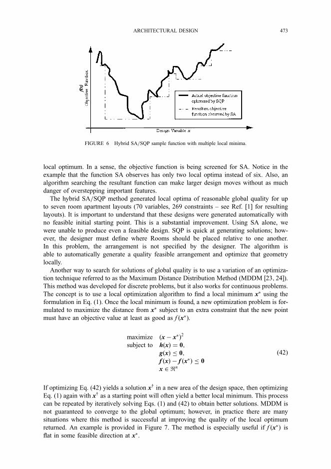
local optimum. In a sense, the objective function is being screened for SA. Notice in the

example that the function SA observes has only two local optima instead of six. Also, an

algorithm searching the resultant function can make larger design moves without as much

danger of overstepping important features.

The hybrid SA=SQP method generated local optima of reasonable global quality for up

to seven room apartment layouts (70 variables, 269 constraints – see Ref. [1] for resulting

layouts). It is important to understand that these designs were generated automatically with

no feasible initial starting point. This is a substantial improvement. Using SA alone, we

were unable to produce even a feasible design. SQP is quick at generating solutions; how-

ever, the designer must define where Rooms should be placed relative to one another.

In this problem, the arrangement is not specified by the designer. The algorithm is

able to automatically generate a quality feasible arrangement and optimize that geometry

locally.

Another way to search for solutions of global quality is to use a variation of an optimiza-

tion technique referred to as the Maximum Distance Distribution Method (MDDM ½23; 24�).

This method was developed for discrete problems, but it also works for continuous problems.

The concept is to use a local optimization algorithm to find a local minimum x� using the

formulation in Eq. (1). Once the local minimum is found, a new optimization problem is for-

mulated to maximize the distance from x� subject to an extra constraint that the new point

must have an objective value at least as good as f ðx�).

maximize ðx� x�Þ2

subject to hðxÞ ¼ 0;gðxÞ � 0;f ðxÞ � f ðx�Þ � 0

x 2 <n

ð42Þ

If optimizing Eq. (42) yields a solution xy in a new area of the design space, then optimizing

Eq. (1) again with xy as a starting point will often yield a better local minimum. This process

can be repeated by iteratively solving Eqs. (1) and (42) to obtain better solutions. MDDM is

not guaranteed to converge to the global optimum; however, in practice there are many

situations where this method is successful at improving the quality of the local optimum

returned. An example is provided in Figure 7. The method is especially useful if f ðx�Þ is

flat in some feasible direction at x�.

FIGURE 6 Hybrid SA=SQP sample function with multiple local minima.


Another design exploration program was written to produce design alternatives by searching

the space using a strategy of random design changes. The program makes design moves of

three types: (1) swap the positions of two Units, (2) perturb the position of a Unit, and (3)

reduce the size of a Unit. After each design move, the program attempts to re-optimize

using the geometric optimization algorithm. The algorithm first attempts to find a feasible

design using penalty methods. If it is unable to find a feasible design, the program makes

one of the three design moves at random. When a feasible design is found, it is saved, and

the program continues by making more random design moves. This strategy was used to

generate designs for a simple three-bedroom apartment layout. The program generated 200

design alternatives overnight. Although this strategy is not rigorous, it is a useful tool for

generating a spread of design alternatives that can be explored further with the interactive

design tool (see Ref. [2]).

3 OPTIMIZATION OF TOPOLOGY

The topology optimization problem is presented as a process of finding the best set of rela-

tionships between rooms in a space. In this formulation, relationships include connectivity,

and initial rough location. Connectivity defines which rooms are directly connected by a

doorway or open pathway. Rough location defines rough arrangement of rooms. Other mod-

els (½9; 10�) have used decision variables to define topological spatial relationships (i.e. adj-

to-north-of, adj-to-south-of, etc:). However, the use of rough room position to describe spa-

tial relationships does not enforce these relationships during geometric optimization, so the

geometric optimization algorithm has more freedom to manipulate the geometry.

Topologies could be evaluated based on topological qualities, such as openness, proximity,

directionality, or symmetry; however, even though these aspects are often thought of as

topological, they are difficult to evaluate without rough geometry. It is best to evaluate

objectives using a geometric layout, therefore each topology is evaluated based on the

FIGURE 7 Demonstration of the MDDM method for finding improved local optima. An initial design (a) wasoptimized using CFSQP. The result is a local optimum (b) (the design cannot be improved by small changes in thedesign variables). The MDDM method was used to generate design (c), an improved local optimum for this example.


best geometry that can be generated from it. Using this method, layouts can be optimized for

any objective that can be formulated in terms of geometry or topology.

Figure 8 shows the topology optimization process. A discrete optimization algorithm uses

information from previous topologies to generate new topologies. Each new feasible topo-

logy, X, is translated into a geometric optimization problem. A locally optimal geometry

x� is found using CFSQP, and the quality of that geometry fgðx�Þ defines the quality

of the topology that generated it, ftðX Þ. The discrete optimization algorithm searches for

the topology that generates the best geometry.

3.1 Mathematical Topology Optimization Model

3.1.1 Variables

The variables for the topology optimization problem are the initial grid position of each

room, and the connectivity between each room and every other room=external wall.

xi; yi 2 Zþ

fij 2 f0; 1g

8 i 2 froomsg; 8 j 2 ðfrooms > ig [ fextwallsgÞ

ð43Þ

where ðxi; yiÞ represents integer Cartesian coordinates of room i, and fij represents the

existence of a connection between room i and room j (or external wall j). Figure 9

FIGURE 8 Building topology optimization method.


shows a visual representation of the design variables. It is important to note that topological

decisions about relative positions of rooms (i.e., room i is-north-of room j) are represented

here using absolute positions of rooms. Several other methods of representing topological

decisions (½9; 10�) do not use absolute positions; however, it is necessary in this strategy

because the geometric optimization algorithm requires a starting design with geometric

information. The use of absolute positions has several consequences: (1) The mapping

from topology to geometry is not injective (one-to-one). It is possible for more than

one topology to generate the same geometry. This means that computation time can be

wasted searching similar topologies. (2) The mapping from topology to geometry is not

surjective (onto). Because each room is represented as a grid point, each topology could

be interpreted geometrically in several ways. It is not clear, however, that every possible

FIGURE 9 A 4-room example showing design variables in the topology formulation. (a) Room position gridshowing (x, y) for each room. Phantom lines show room connections. The dashed line shows the implied boundary.


geometric alternative can be generated using the topology definition in this paper. (3) The

space of topology combinations is exponential.

Because of these limitations, this representation is not well suited to problems where all

solutions need to be enumerated. It is not clear that the representation can enumerate all pos-

sible topology alternatives; however, this method is powerful for larger problems where heur-

istic search is necessary. This is because in practice heuristic search algorithms can often find

reasonable quality designs quickly, while enumeration algorithms must systematically

explore designs one by one, which can often take too long to be practical.

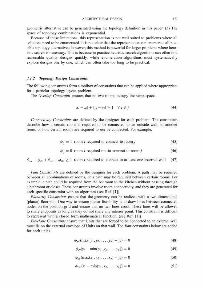
3.1.2 Topology Design Constraints

The following constraints form a toolbox of constraints that can be applied where appropriate

for a particlar topology layout problem.

The Overlap Constraint ensures that no two rooms occupy the same space.

jxi � xjj þ jyi � yjj � 1 8 i 6¼ j ð44Þ

Connectivity Constraints are defined by the designer for each problem. The constraints

describe how a certain room is required to be connected to an outside wall, to another

room, or how certain rooms are required to not be connected. For example,

fij ¼ 1 room i required to connect to room j ð45Þ

fij ¼ 0 room i required not to connect to room j ð46Þ

fiN þ fiS þ fiE þ fiW � 1 room i required to connect to at least one external wall ð47Þ

Path Constraints are defined by the designer for each problem. A path may be required

between all combinations of rooms, or a path may be required between certain rooms. For

example, a path could be required from the bedroom to the kitchen without passing through

a bathroom or closet. These constraints involve room connectivity, and they are generated for

each specific constraint with an algorithm (see Ref. [1]).

Planarity Constraints ensure that the geometry can be realized with a two-dimensional

(planar) floorplan. One way to ensure planar feasibility is to draw lines between connected

nodes on the position grid and ensure that no two lines cross. These lines will be allowed

to share endpoints as long as they do not share any interior point. This constraint is difficult

to represent with a closed form mathematical function. (see Ref. [1])

Envelope Constraints ensure that Units that are forced to be connected to an external wall

must lie on the external envelope of Units on that wall. The four constraints below are added

for each unit i

fiN ðmaxð y1; y2; . . . ; ynÞ � yiÞ ¼ 0 ð48Þ

fiSðyi � minð y1; y2; . . . ; ynÞÞ ¼ 0 ð49Þ

fiEðmaxðx1; x2; . . . ; xnÞ � yiÞ ¼ 0 ð50Þ

fiW ðxi � minðx1; x2; . . . ; xnÞÞ ¼ 0 ð51Þ


3.1.3 Objective

The objective of the topology optimization problem is to minimize the objective value of the

resultant local optimal geometry formed by the topology.

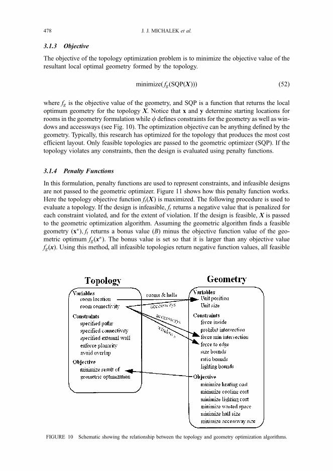
minimizeð fgðSQPðX ÞÞÞ ð52Þ

where fg is the objective value of the geometry, and SQP is a function that returns the local

optimum geometry for the topology X. Notice that x and y determine starting locations for

rooms in the geometry formulation while f defines constraints for the geometry as well as win-

dows and accessways (see Fig. 10). The optimization objective can be anything defined by the

geometry. Typically, this research has optimized for the topology that produces the most cost

efficient layout. Only feasible topologies are passed to the geometric optimizer (SQP). If the

topology violates any constraints, then the design is evaluated using penalty functions.

3.1.4 Penalty Functions

In this formulation, penalty functions are used to represent constraints, and infeasible designs

are not passed to the geometric optimizer. Figure 11 shows how this penalty function works.

Here the topology objective function ftðX Þ is maximized. The following procedure is used to

evaluate a topology. If the design is infeasible, ft returns a negative value that is penalized for

each constraint violated, and for the extent of violation. If the design is feasible, X is passed

to the geometric optimization algorithm. Assuming the geometric algorithm finds a feasible

geometry ðx�Þ; ft returns a bonus value (B) minus the objective function value of the geo-

metric optimum fgðx�Þ. The bonus value is set so that it is larger than any objective value

fgðxÞ. Using this method, all infeasible topologies return negative function values, all feasible

FIGURE 10 Schematic showing the relationship between the topology and geometry optimization algorithms.


topologies return positive objective function values, and feasible topologies that result in bet-

ter geometries (lower fgðxÞ) have a better objective function value (higher ftðX Þ).

3.2 Topology Model Solution Method

The discrete topology design space is combinatorial, multi-modal, and highly constrained, so

it must be searched with a global scope. The space of topologies could be searched exhaus-

tively with a constraint satisfaction programming enumeration algorithm [27] or branch and

bound; however, combinatorial explosion will cripple the algorithm for problems of signifi-

cant size. Furthermore, enumeration is unnecessary in a problem where many of the implicit

design goals (such as aesthetic intent) are not generally defined mathematically, but instead

must be judged. It is not meaningful to produce a strict global optimum; instead, it is more

useful to produce an array of quality design alternatives to explore. For this reason, evolu-

tionary algorithms were selected. Evolutionary algorithms search heuristically, and they

can be stopped at any point during the optimization process to return a population of best

designs found. This heuristic search, combined with penalty functions, can often find quality

feasible designs to large problems that are intractable for systematic search methods.

An evolutionary algorithm for topology layout was implemented using the GAlib optimi-

zation package [28]. A SteadyStateGA was selected. A Roulette Wheel selector was used to

select high quality designs with greater probability than low quality designs. When sexual

crossover is used (randomly), two parents are selected from the population, and two new chil-

dren are produced using mixed room connectivity from both parents. When asexual crossover

is used (randomly), one parent is selected from the population, and one new child is produced

by swapping connectivity values between rooms or by swapping room positions. After cross-

over, new designs are mutated slightly. Room locations (x,y) are incremented or connecti-

vities are flipped with low probability.

The evolutionary algorithm implementation is able to generate quality feasible designs for

medium-sized problems.

FIGURE 11 Formulation of the topology objective function.


4 DEMONSTRATION EXAMPLE

A realistic problem was implemented to test the scalability of the automated building genera-

tion algorithm. The example involves a small apartment complex with three separate apart-

ments. Rooms and specifications are shown in Table I. Constraints that are specific to this

problem are listed in Table II. This problem was run for 20,000 generations (100 designs

each generation) to search for global solutions. Feasible designs take much longer to evaluate

than infeasible designs (because feasible designs are passed to the geometric optimization

algorithm), so a second termination criterion was added to terminate after 50 feasible designs

were found. This criterion was intended to make search time more consistent between runs.

The sample topology and resulting geometry solution shown in Figure 12 were generated

using the automated design tool.

TABLE I Room Specifications for Demonstration Problem.

Apt RoomMin. area(sq. ft.)

Min. length and width( ft.)

Max. length andwidth ( ft.)

– Public Entry 9 3 1001 Living Room 160 12 401 Dining Room 100 10 301 Kitchen 100 8 401 Bedroom 120 10 401 Bathroom 30 5 202 Living Room 160 12 402 Dining Room 100 10 302 Kitchen 100 8 402 Bedroom 1 120 10 402 Bedroom 2 120 10 402 Bathroom 30 5 203 Living Room 160 12 403 Dining Room 100 10 303 Kitchen 100 8 403 Bedroom 1 120 10 403 Bedroom 2 120 10 403 Bathroom 30 5 20

TABLE II Topology Specifications for Demonstration Problem.

Constraint type Constraint

Overlap No two Units can occupy the same spaceConnectivity Public Entry must connect to the Living Room of each apartmentConnectivity Public Entry must connect to an external wallConnectivity All bedrooms must connect to an external wallPath In each apartment, there must be a path from the Kitchen to the

Living Room that may pass through the Dining RoomPath In each apartment, there must be a path from the Bathroom to the

Living Room that may pass through the Dining Room and KitchenPath In each apartment, there must be a path from the Dining Room to the

Living Room that may pass through the KitchenPath In each apartment, there must be a path from each Bedroom to the

Living Room that may pass through the Dining RoomAccessways Accessway lines connecting Units cannot intersectEnvelope Units that are connected to an external wall must lie on the boundary

envelope of rooms


The algorithm generates local optimal solutions, but the global search is quite limited due

to combinatorial complexity. Once a feasible topology is found, it has a much higher prob-

ability of being selected as a parent design by the evolutionary algorithm because it has a

much higher fitness value than infeasible designs. Thus, new designs tend to be very similar

to the first feasible design found, and other designs are usually discarded. The result is that

the algorithm tends to fixate on the first feasible solution it finds, exploring mostly variations

of that solution. The algorithm can be run several times to produce design alternatives, but

generally when it is run once, the final population converges to variations of one main design

theme. This is a serious limitation for global search, and the algorithm is more useful as a

feasible-design-finder than as a true optimizer. For smaller problems, the evolutionary algo-

rithm is still able to search a significant range of the design space to find global quality solu-

tions. For this problem, the evolutionary algorithm can consistently find solutions in under

20,000 generations (2 � 106 design evaluations).

The geometric optimization problem does not have the same combinatorial nature that the

topology problem has, and it is able to handle much larger problems. The example shown

in Figure 4, contains 23 rooms, three hallways, one boundary, and 25 accessways for a

total of 52 units. This geometric optimization problem contains 312 variables and 1578 con-

straints.

FIGURE 12 Sample design topology and final geometry generated by the automated design tool.


5 CONCLUSIONS

Two automated optimization algorithms have been used to automate the generation of design

layouts: the geometry and topology algorithms. The geometry algorithm, built on rigorous

gradient-based algorithms, is efficient and robust, and has been successful at optimizing geo-

metry for large problems. In its present state, it is most useful as an aid for design explora-

tion, rather than design automation, because results are highly dependent on the starting point

defined by the designer. Several tools have been implemented for searching the geometric

space more globally, including a hybrid SA=SQP algorithm and a strategic programming

method. These tools have been successful at automatically finding alternative arrangements

for rooms and exploring many local minima.

A second topology optimization algorithm was built on top of the geometric algorithm to

search feasible topology alternatives and find the feasible topology that generates the best

geometry. The results are interesting, but limited. One advantage to the approach presented

here is that the final design generated by the algorithm can be used as a starting point for

interactive design exploration (see Ref. [2]).

Possible improvements include the addition of new shapes, objectives, and constraints to

the design toolbox to address more complex geometry, material selection, building codes,

structural elements, routing of wires, pipes and ducts, and more accurate models.

Additionally, the topology search can be improved if the topology can be defined in a new

FIGURE 12 (Continued)


way so that topology decisions create linear constraints in the geometry optimization pro-

blem. Using a different definition of topology, such as in Refs. [3–5], it is possible to elim-

inate the rough position topology variables, and ensure that the mapping from topology to

local optimal geometry is both injective and surjective (meaning that each valid topology

will create a different locally optimal geometries, and that all possible local optimal geometry

could be created by a specific topology).

Acknowledgements

Special thanks to Professor Kazuhiro Saitou, John Whitehead, Panayiotis Georgiopoulos, and

Adam Cooper for their contributions to the topology optimization model and solution

strategy.

References

[1] Michalek, J. (2001). Interactive layout design optimization. MS thesis, University of Michigan.[2] Michalek, J. and Papalambros, P. Y. (2002). Interactive design optimization of architectural layouts. Engineering

Optimization (this issue).[3] Levin, P. H. (1964). Use of graphs to decide the optimum layout of buildings. Architect, 14, 809–815.[4] Liggett, R. S. and Mitchell, W. J. (1981). Optimal space planning in practice. Computer-Aided Design, 13(5),

277–288.[5] Sharpe, R., Marksjo, B. S., Mitchell, J. R. and Crawford, J. R. (1985). An interactive model for the layout of

buildings. Applied Mathematical Modeling, 9, 207–214.[6] Jo, J. H. and Gero, J. S. (1998). Space layout planning using an evolutionary approach. Artificial Intelligence

in Engineering, 12, 149–162.[7] Jagielski, R. and Gero, J. S. (1997). A genetic programming approach to the space layout planning problem.

CAAD Futures, 875–884.[8] Baykan, C. A. and Fox, M. S. (1997). Spatial synthesis by disjunctive constraint satisfaction. Artificial

Intelligence in Engineering Design, 11, 245–262.[9] Schwarz, A., Berry, D. M. and Shaviv, E. (1994). Representing and solving the automated building design

problem. Computer-Aided Design, 26(9), 689–698.[10] Medjdoub, B. and Yannou, B. (1999). Separating topology and geometry in space planning. Computer-Aided

Design, 32, 39–61.[11] Yin, S. and Cagan, J. (2000). An extended pattern search algorithm for three-dimensional component layout.

Transactions of the ASME, 122, 102–108.[12] Cagan, J., Degentesh, D. and Yin, S. (1998). A simulated annealing-based algorithm using hierarchical models

for general three-dimensional component layout. Computer-Aided Design, 30(10), 781–790.[13] Szykman, S. and Cagan, J. (1997). Constrained three-dimensional component layout using simulated annealing.

ASME Transactions, 119, 28–35.[14] Choo, H. J. and Tommelein, I. D. (1999). Space scheduling using flow analysis. Proc. Seventh Annual

Conference of the International Group for Lean Construction, 299–312.[15] Rong, B. (1997). Automated generation of fixture configuration design. Journal of Manufacturing Science and

Engineering, 119, 208–219.[16] Koide, T. and Wakabayashi, S. (1999). A timing-driven floorplanning algorithm with the Elmore delay model for

building block layout. Integration, the VLSI Journal, 27, 57–76.[17] Wang, Y. and Wu, H. (1998). Method of constraint graphs used in spatial layout. Ruan Jian Xue Bao Journal

of \Software, 9(3), 200–205.[18] Ito, T. (1999). A genetic algorithm approach to piping route path planning. Journal of Intelligent Manufacturing,

10, 103–114.[19] Fadel, G. M., Sinha, A. and McKee, T. (2001). Packing optimisation using a rubberband analogy. Proceedings of

DETC’01 2001, ASME Design Engineering Technical Conferences, DETC2001=DAC-21051.[20] Kim, J. J. and Gossard, D. C. (1991). Reasoning on the location of components for assembly packaging. Journal

of Mechanical Design, Transactions of the ASME, 113(4), 402–407.[21] Chapman, C. D., Saitou, K. and Jakiela, M. J. (1994). Genetic algorithms as an approach to configuration and

topology Design. Journal of Mechanical Design, Transactions of the ASME, 116(4), 1005–1012.[22] Papalambros, P. Y. and Wilde, D. J. (2000). Principles of Optimal Design–Modeling and Computation, 2nd ed.

Cambridge University Press, Cambridge, England.[23] Kott, G. J. and Gabriele, G. (1998). A tunnel based method for mixed discrete constrained nonlinear

optimization. ASME Design Automation Conference, DETC98=DAC-5592.[24] Kott, G. J. (1998). A method for mixed variable constrained nonlinear optimization based on a new function

bounding technique. PhD thesis, Rensselaer Polytechnic Institute.


[25] Zhou, J. L. and Tits, A. L. (1995). An SQP algorithm for finely discretized continuous minimax problems andother minimax problems with many objective functions. SIAM Journal of Optimization, 6, 461–487.

[26] Lawrence, C. T., Zhou, J. L. and Tits, A. (1995). User’s guide for CFSQP version 2.3: A C code for solving largescale constrained nonlinear minimax optimization problem, generating iterates satisfying all inequalityconstraints. Institute for Systems Research, University of Maryland, Technical Report TR-94-16r1.

[27] Bartak, R. (1999). Constraint programming: In pursuit of the Holy Grail. http:==kti.ms.mff.cuni.cz=�bartak=constraints.

[28] Wall, M. (1996). GAlib: A Cþ þ library of genetic algorithm components-Version 2.4 -Document revision [email protected], http:==lancet.mit.edu=ga=dist=galibdoc.pdf.

[29] Bentley, P. J. (1999). Evolutionary Design by Computers.Morgan Kaufmann Publishers, Inc., San Francisco, CA.[30] ASHRAE (1997). Fundamentals. American Society of Refrigeration, Heating and Air-conditioning Engineers,

Atlanta, GA.[31] IESNA (1998). IESNA Lighting Education: Intermediate Level. Illumination Engineers Society of North

America.


architectural layout design optimization fileeng. opt., 2002, vol. 34(5), pp. 461–484...

Documents