1

Approximate Analysis of Statically Indeterminate

Structures

Every successful structure must be capable of reaching stable equilibrium under its applied loads, regardless of structural behavior. Exact analysis of indeterminate structures involves computation of deflections and solution of simultaneous equations. Thus, computer programs are typically used.

2

To eliminate the difficulties associated with exact analysis, preliminary designs of indeter-minate structures are often based on the results of approximate analysis.

Approximate analysis is based on introducing deformation and/or force distribution assumptions into a statically indeterminate structure, equal in number to degree of indeter-minacy, which maintains stable equilibrium of the structure.

3

No assumptions inconsistent with stable equilibrium are admissible in any approximate analysis.

Uses of approximate analysisinclude:

(1) planning phase of projects, when several alternative designs of the structure are usually evaluated for relative economy;

(2) estimating the various member sizes needed to initiate an exact analysis;

4

(3) check on exact analysis results;

(4) upgrades for older structure designs initially based on approximate analysis; and

(5) provide the engineer with a sense of how the forces distribute through the structure.

5

In order to determine the reac-tions and internal forces for indeterminate structures using approximate equilibrium me-thods, the equilibrium equations must be supplemented by enough equations of conditions or assumptions such that the resulting structure is stable and statically determinate.

6

The required number of such additional equations equals the degree of static indeter-minacy for the structure, with each assumption providing an independent relationship between the unknown reactions and/or internal forces.

In approximate analysis, these additional equations are based on engineering judgment of appropriate simplifying assump-tions on the response of the structure.

7

Approximate Analysis of a Continuous Beam for Gravity Loads

Continuous beams and girders occur commonly in building floor systems and bridges. In the approximate analysis of con-tinuous beams, points of inflection or inflection point (IP) positions are assumed equal in number to the degree of static indeterminacy.

8

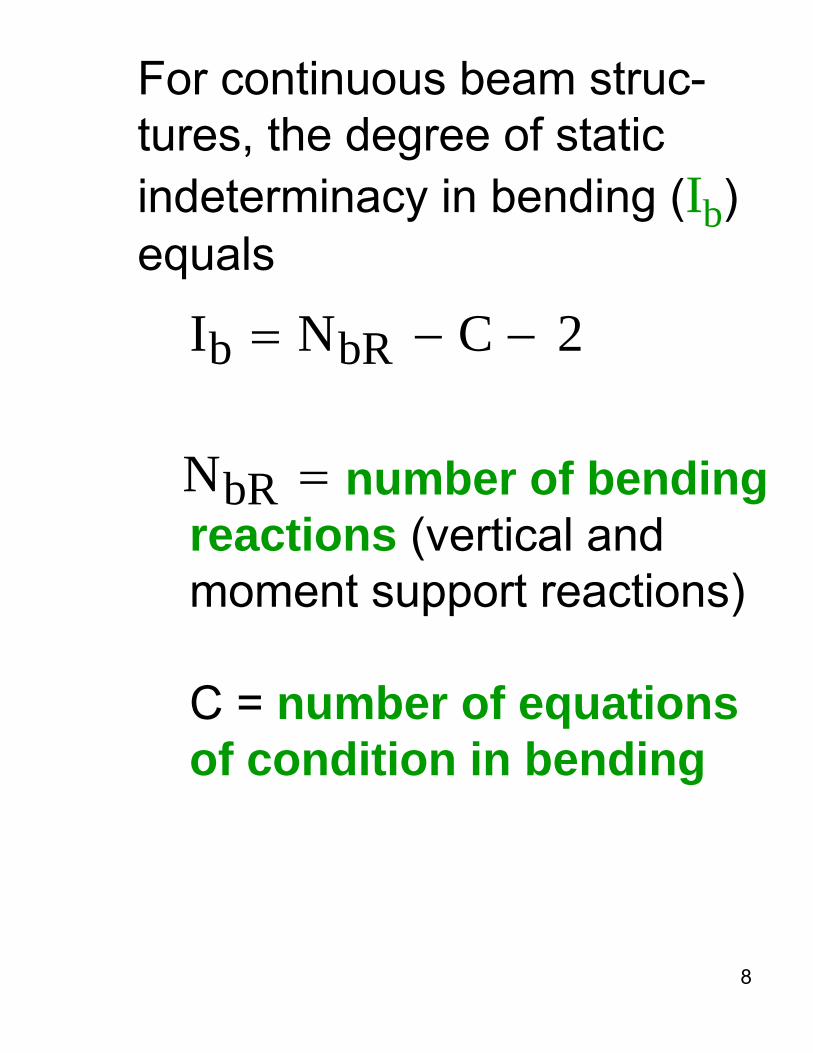
For continuous beam struc-tures, the degree of static indeterminacy in bending (Ib) equals

number of bending reactions (vertical and moment support reactions)

C = number of equations of condition in bending

b bRI N C 2= − −

bRN =

9

Each inflection point position introduces one equation of condition to the static equilibri-um equations. Three strategies are used to approximate the location of the inflection points:

1. qualitative displacement diagrams of the beam structure,

2. qualitative bending moment diagrams (preferred method for students), and

3. location of exact inflection points for some simple statically indeterminate structures.

10

Approximate analysis of con-tinuous beams using the quali-tative deflection diagram is based on the fact that the elastic curve (deflected shape) of a continuous beam can generally be sketched with a fair degree of accuracy without performing an exact analysis. When the elastic curve is sketched in this manner, the actual magnitudes of deflec-tion (displacements and rota-tions) are not accurately por-trayed, but the inflection point locations are easily estimated even on a fairly rough sketch.

11

Qualitative bending moment diagrams can also be used to locate inflection points. Bending moments in spans with no loading are linear or constant; with point loading the span bending moment equations are piecewise linear; and with uniform loading the moments are quadratic. Remember, internal bending moments at interior support locations adjacent to one or two loaded spans is negative.

Recall that zero moment locations correspond to the inflection point locations.

12

From the total set of inflection points, select the needed number to achieve a solution by statics.

In the case of beams, there will normally be enough inflection points to reduce the structure to a statically determinate structure and typically there are more inflection points than the degree of indeterminacy.

13

With the inflection points located (equal in number to the degree of static indeterminacy), the analysis can proceed on the basis of statics alone. Since an inflection point is a zero moment location, it may be thought of as an internal hinge for purposes of analysis.

Some examples to guide the “learning” and “practice” are given on the following pages. Both the elastic curve and bending moment diagrams are given.

14

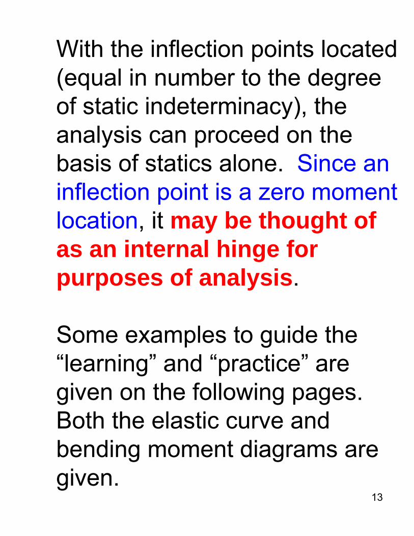
Fixed-Fixed Beam Subjected to a Uniform Load

15

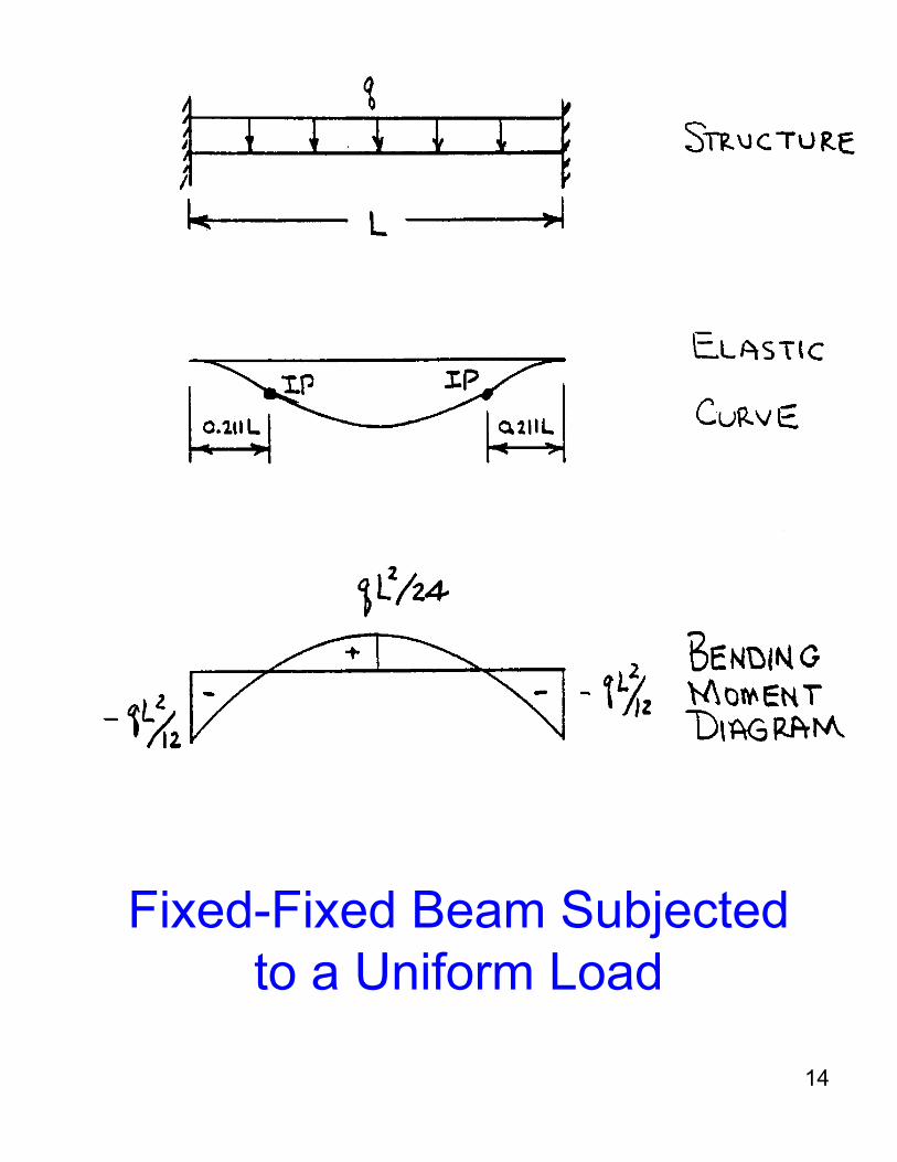
Fixed-Fixed Beam Subjected to a Central Point Force

16

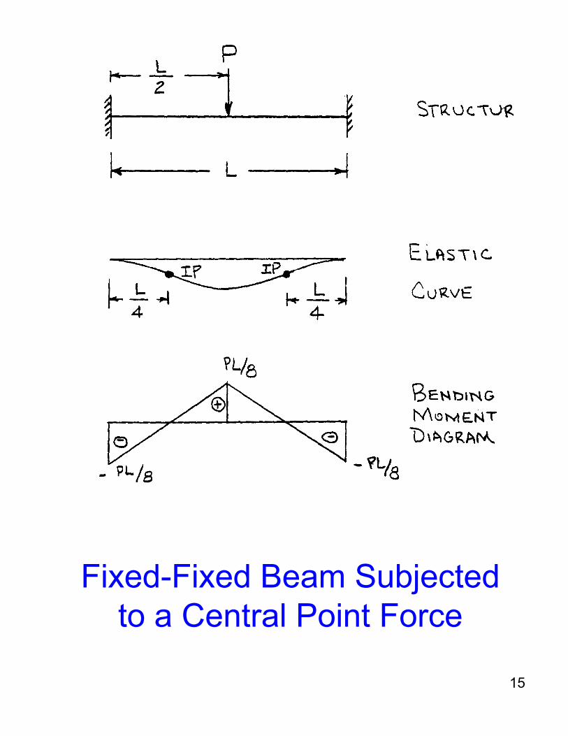
Propped Cantilever Beam Subjected to a Uniform Load

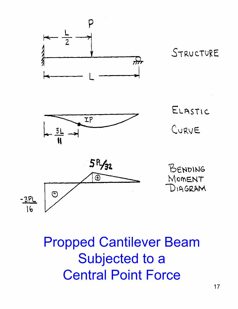
17

Propped Cantilever Beam Subjected to a

Central Point Force

18

When considering problems that do not match the exact values given, some useful guides are:

•Inflection points move towards positions of reduced stiffness,

•No more than one inflection point can occur in an un-loaded span, and

•No more than two inflection points will occur in a loaded span.

19

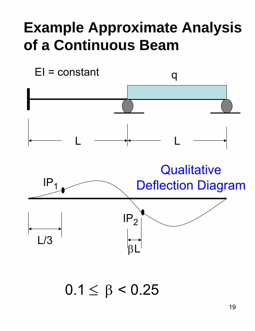
Example Approximate Analysis of a Continuous Beam

L L

qEI = constant

IP1

IP2

L/3βL

0.1 β < 0.25≤

Qualitative Deflection Diagram

20

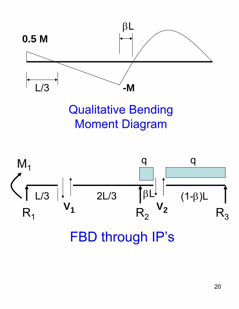
Qualitative Bending Moment Diagram

-M

0.5 M

L/3

βL

L/3 2L/3 βL (1-β)LV1 V2R1

M1

R2 R3

FBD through IP’s

q q

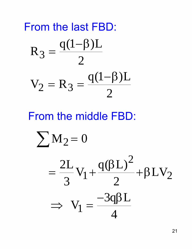
21

3

2 3

q(1 )LR2

q(1 )LV R2

−β=

−β= =

From the last FBD:

From the middle FBD:

21 2

1

2L q( L)V LV3 2

3q LV4

β= + +β

− β⇒ =

2M 0=∑

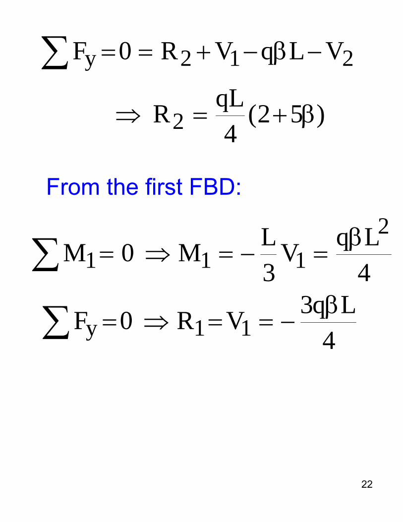
22

From the first FBD:

y 2 1 2F 0 R V q L V= = + − β −∑

2qLR (2 5 )4

⇒ = + β

21 1 1

L q LM 0 M V3 4

β= ⇒ = − =∑

y 1 13q LF 0 R V

4β= ⇒ = = −∑

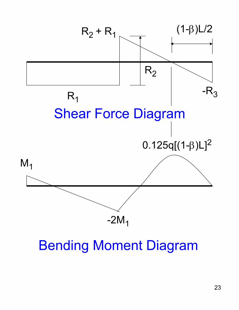
23

Shear Force DiagramR1

R2

-R3

R2 + R1

M1

-2M1

0.125q[(1-β)L]2

(1-β)L/2

Bending Moment Diagram

24

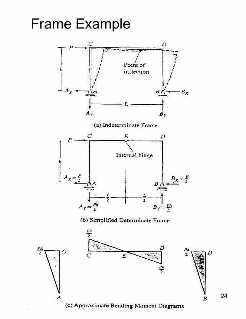
Frame Example

25

Trusses with Double Diagonals

Truss systems for roofs, bridges and building walls often contain double diagonals in each panel, which makes each panel statically indeterminate.

Approximate analysis requires that the number of assump-tions introduced must equal the degree of indeterminacy so that only the equations of equi-librium are required to perform the approximate analysis.

26

Since one extra diagonal exists in each double diagonal panel, one assumption regarding the force distribution between the two diagonals must be made in each panel. If the diagonals are slender, it may be assumed that the diagonal members are only capable of resisting tensile forces and that diagonals subjected to compression can be ignored since they are susceptible to buckling, i.e., assume very small buckling load and ignore post-buckling strength.

27

Such an assumption is illustrated in Fig. DD.1(a). In Fig. DD.1(a), the total panel shear is assumed to be resisted by the tension diagonal as shown. Compres-sion diagonals are assumed to resist no loading. With this assumption, the truss of Fig. DD.1 is statically determinate.

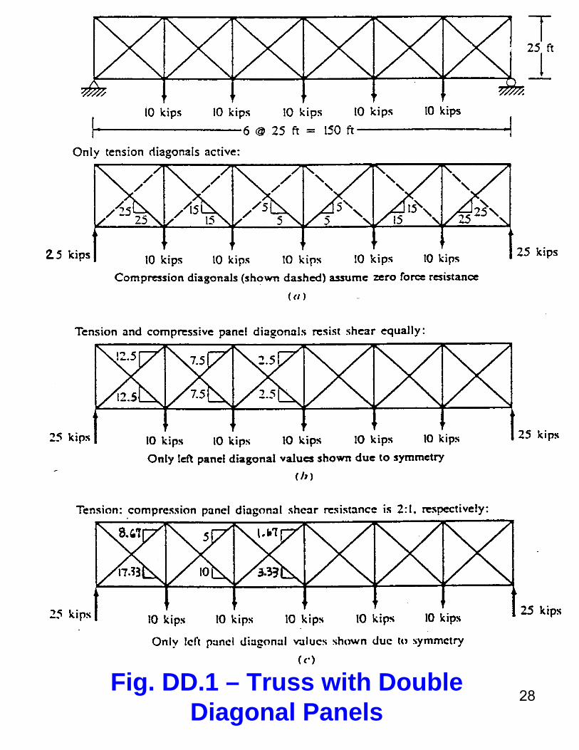
28Fig. DD.1 – Truss with Double

Diagonal Panels

29

The assumption discussed in the previous paragraph is generally too stringent, i.e., the compres-sion diagonals can resist a portion of the panel shear.

Figures DD.1(b) and (c) show two different assumptions regarding the ability of the compression diagonals to resist force.

30

Figure DD.1(b) shows the shear (vertical) components of the diagonal members assuming that the compression and tension diagonals equally resist the panel shear.

Figure DD.1(c) shows the vertical force distribution among the compression and tension diagonals based on the tension diagonal resisting twice the force of the compression diagonal or two-thirds of the panel shear.

31

Any reasonable assumption can be made.

The compression diagonal assumptions for double diagonal trusses can be mathematically summarized as:

C = αT; 0 ≤ α ≤ 1

If PS = Panel Shear, then

T(1+α) = PS

32

Once the diagonal member forces are determined, the remaining member forces in the truss can be calculated using simple statics, i.e., the method of sections and/or the method of joints.