approval sheet - csee.umbc.edu
TRANSCRIPT


APPROVAL SHEET Title of Dissertation: BayesOWL: A Probabilistic Framework for
Uncertainty in Semantic Web Name of Candidate: Zhongli Ding Doctor of Philosophy, 2005 Dissertation and Abstract Approved: ______________________________
Yun Peng, Ph.D. Associate Professor Department of Computer Science and Electrical Engineering
Date Approved: ________________________
Curriculum Vitae Name: Zhongli Ding. Permanent Address: 3207-310 West Springs Dr., Ellicott City, MD 21043. Degree and Date to be Conferred: Ph.D., December 2005. Date of Birth: December 7, 1976. Place of Birth: Yiwu, Zhejiang, People’s Republic of China. Secondary Education:
Guiyang No.1 High School Guizhou Province, People’s Republic of China, June 1994
Collegiate Institutions Attended: University of Maryland, Baltimore County, Baltimore, Maryland September 2001 – December 2005, Ph.D., December 2005 Major: Computer Science University of Maryland, Baltimore County, Baltimore, Maryland September 1999 – May 2001, M.S., May 2001 Major: Computer Science University of Science and Technology of China, Hefei, Anhui, China September 1994 – July 1999, B.S., July 1999 Major: Computer Science Professional Publications: Z. Ding, BayesOWL: A Probabilistic Framework for Uncertainty in Semantic Web, Computer Science Doctoral Dissertation, University of Maryland, Baltimore County, December 2005.

Z. Ding, Y. Peng, and R. Pan: “BayesOWL: Uncertainty Modeling in Semantic Web Ontologies”, book chapter to be appeared in “Soft Computing in Ontologies and Semantic Web”, to be published by Springer-Verlag, in the series “Studies in Fuzziness and Soft Computing”. L. Ding, P. Kolari, Z. Ding, and S. Avancha: “Using Ontologies in the Semantic Web: A Survey”, book chapter to be appeared in “Ontologies in the Context of Information Systems”, to be published by Springer-Verlag, Oct. 15, 2005. (Also as UMBC Technical Report TR-CS-05-07, July 2005.) R. Pan, Z. Ding, Y. Yu, and Y. Peng: “A Bayesian Network Approach to Ontology Mapping”, to be appeared in the Proceedings of ISWC 2005. Galway, Ireland, Nov. 6 – Nov. 10, 2005. Y. Peng and Z. Ding: “Modifying Bayesian Networks by Probability Constraints”, in the Proceedings of UAI 2005. Edinburgh, Scotland, July 26 – July 29, 2005. Z. Ding, Y. Peng, R. Pan, and Y. Yu: “A Bayesian Methodology towards Automatic Ontology Mapping”, in the Proceedings of First International Workshop on “Contexts and Ontologies: Theory, Practice and Applications”, held in AAAI-05. Pittsburgh, PA, July 9, 2005. Z. Ding, Y. Peng, and R. Pan: “A Bayesian Approach to Uncertainty Modeling in OWL Ontology”, in the Proceedings of 2004 International Conference on Advances in Intelligent Systems - Theory and Applications (AISTA2004). Luxembourg, Nov. 2004. Z. Ding and Y. Peng: “A Probabilistic Extension to Ontology Language OWL”, in the Proceedings of the 37th Hawaii International Conference on System Sciences (HICSS-37). Big Island, Hawaii, Jan. 2004. L. Ding, T. Finin, Y. Shi, Y. Zou, Z. Ding, and R. Pan: “Strategies and Heuristics used by the UMBCTAC Agent in the third Trading Agent Competition”, in the Workshop on “Trading Agent Design and Analysis”, held in IJCAI-2003. Acapulco, Mexico, Aug. 2003.
L. Ding, Y. Shi, Z. Ding, R. Pan, and T. Finin: “UMBCTAC: A Balanced Bidding Agent”. UMBC Technical Report TR-02-15, 2002. Professional Positions Held: September 1999 ~ August 2005, Graduate Assistant, CSEE, UMBC.

Abstract Title of Dissertation: BayesOWL: A Probabilistic Framework for Uncertainty in
Semantic Web Zhongli Ding, Doctor of Philosophy, 2005 Dissertation directed by:
Yun Peng Associate Professor Department of Computer Science and Electrical Engineering University of Maryland, Baltimore County
To address the difficult but important problem of modeling uncertainty in semantic web,
this research takes a probabilistic approach and develops a theoretical framework, named
BayesOWL, that incorporates the Bayesian network (BN), a widely used graphic model
for probabilistic interdependency, into the web ontology language OWL. This framework
consists of three key components: 1) a representation of probabilistic constraints as OWL
statements; 2) a set of structural translation rules and procedures that converts an OWL
taxonomy ontology into a BN directed acyclic graph (DAG); and 3) a method SD-IPFP
based on “iterative proportional fitting procedure” (IPFP) that incorporates available
probability constraints into the conditional probability tables (CPTs) of the translated BN.
The translated BN, which preserves the semantics of the original ontology and is
consistent with all the given probability constraints, can support ontology reasoning, both
within and cross ontologies, as Bayesian inferences, with more accurate and more
plausible results.
SD-IPFP was further developed into D-IPFP, a general approach for modifying BNs
with probabilistic constraints that goes beyond BayesOWL. To empirically validate this

theoretical work, both BayesOWL and variations of IPFP have been implemented and
tested with example ontologies and probabilistic constraints. The tests confirmed
theoretical analysis.
The major advantages of BayesOWL over existing methods are: 1) it is non-intrusive and
flexible, neither OWL nor ontologies defined in OWL need to be modified and one can
translate either the entire ontology or part of it into BN depending on the needs; 2) it
separates the “rdfs:subClassOf” relations (or the subsumption hierarchy) from other
logical relations by using L-Nodes, which makes CPTs of the translated BN smaller and
easier to construct in a systematic and disciplined way, especially in a domain with rich
logical relations; 3) it does not require availability of complete conditional probability
distributions, pieces of probability information can be incorporated into the translated BN
in a consistent fashion. One thing to emphasize is that BayesOWL can be easily extended
to handle other ontology representation formalisms (syntax is not important, semantic
matters), if not using OWL.

BayesOWL: A Probabilistic Framework
for Uncertainty in Semantic Web
by Zhongli Ding
Dissertation submitted to the Faculty of the Graduate School of the University of Maryland in partial fulfillment
of the requirements for the degree of Doctor of Philosophy
2005

© Copyright Zhongli Ding 2005


ii
To all my family members, for supporting me and loving me all the time.

Table of Contents
List of Tables . . . . . . . . . . . . . . . . . . . . . . . . . . . . . . . . . v
List of Figures . . . . . . . . . . . . . . . . . . . . . . . . . . . . . . . . vi
1 Introduction . . . . . . . . . . . . . . . . . . . . . . . . . . . . . . . . 1
1.1 The Motivations . . . . . . . . . . . . . . . . . . . . . . . . . . . . . . 2
1.2 Thesis Statement . . . . . . . . . . . . . . . . . . . . . . . . . . . . . 4
1.3 Dissertation Outline . . . . . . . . . . . . . . . . . . . . . . . . . . . 7
2 Background and Related Works . . . . . . . . . . . . . . . . . . . . 9
2.1 Ontology and Semantic Web . . . . . . . . . . . . . . . . . . . . . . . 9
2.1.1 The Semantic Web . . . . . . . . . . . . . . . . . . . . . . . . 10
2.1.2 What is Ontology? . . . . . . . . . . . . . . . . . . . . . . . . 12
2.1.3 Brief Introduction to Description Logics . . . . . . . . . . . . 16
2.2 Bayesian Belief Networks . . . . . . . . . . . . . . . . . . . . . . . . . 21
2.2.1 Definition and Semantics . . . . . . . . . . . . . . . . . . . . . 21
2.2.2 Inference . . . . . . . . . . . . . . . . . . . . . . . . . . . . . . 25
2.2.3 Learning . . . . . . . . . . . . . . . . . . . . . . . . . . . . . . 26
2.3 Uncertainty for the Semantic Web . . . . . . . . . . . . . . . . . . . . 28
2.3.1 Uncertainty Modeling and Reasoning . . . . . . . . . . . . . . 29
2.3.2 Representation of Probabilistic Information . . . . . . . . . . 34
2.4 IPFP: Iterative Proportional Fitting Procedure . . . . . . . . . . . . 35
2.4.1 The ABCs of Probability . . . . . . . . . . . . . . . . . . . . . 36
2.4.2 IPFP and C-IPFP . . . . . . . . . . . . . . . . . . . . . . . . 41
2.5 Other Related Works . . . . . . . . . . . . . . . . . . . . . . . . . . . 42
iii

2.5.1 Ontology-Based Semantic Integration . . . . . . . . . . . . . . 44
2.5.2 Database Schema Integration . . . . . . . . . . . . . . . . . . 48
2.6 Summary . . . . . . . . . . . . . . . . . . . . . . . . . . . . . . . . . 50
3 Modifying Bayesian Networks by Probabilistic Constraints . . . . 52
3.1 Preliminaries . . . . . . . . . . . . . . . . . . . . . . . . . . . . . . . 55
3.2 The Problem of Modifying BNs with Probabilistic Constraints . . . . 61
3.3 E-IPFP . . . . . . . . . . . . . . . . . . . . . . . . . . . . . . . . . . 64
3.4 D-IPFP . . . . . . . . . . . . . . . . . . . . . . . . . . . . . . . . . . 67
3.5 SD-IPFP . . . . . . . . . . . . . . . . . . . . . . . . . . . . . . . . . . 75
3.6 The IPFP API . . . . . . . . . . . . . . . . . . . . . . . . . . . . . . 77
3.7 Experiments . . . . . . . . . . . . . . . . . . . . . . . . . . . . . . . . 78
3.8 Summary . . . . . . . . . . . . . . . . . . . . . . . . . . . . . . . . . 82
4 BayesOWL - A Probabilistic Extension to OWL . . . . . . . . . . 85
4.1 Representing Probabilistic Information . . . . . . . . . . . . . . . . . 86
4.2 Structural Translation . . . . . . . . . . . . . . . . . . . . . . . . . . 88
4.3 CPT Construction . . . . . . . . . . . . . . . . . . . . . . . . . . . . 92
4.4 Semantics of BayesOWL . . . . . . . . . . . . . . . . . . . . . . . . . 99
4.5 Reasoning . . . . . . . . . . . . . . . . . . . . . . . . . . . . . . . . . 102
4.6 The OWL2BN API . . . . . . . . . . . . . . . . . . . . . . . . . . . . 106
4.7 Comparison to Existing Works . . . . . . . . . . . . . . . . . . . . . . 108
4.8 Summary . . . . . . . . . . . . . . . . . . . . . . . . . . . . . . . . . 113
5 Conclusion and Future Work . . . . . . . . . . . . . . . . . . . . . . 115
Appendix . . . . . . . . . . . . . . . . . . . . . . . . . . . . . . . . . . . 127
References . . . . . . . . . . . . . . . . . . . . . . . . . . . . . . . . . . . 133
iv

List of Tables
3.1 The E-IPFP Algorithm . . . . . . . . . . . . . . . . . . . . . . . 66
3.2 The D-IPFP Algorithm . . . . . . . . . . . . . . . . . . . . . . . 70
4.1 Representing P (c) = 0.8 in OWL . . . . . . . . . . . . . . . . . . 87
4.2 Representing P (c|p1, p2, p3) = 0.8 in OWL . . . . . . . . . . . . . 88
4.3 Supported Constructors . . . . . . . . . . . . . . . . . . . . . . . 89
4.4 CPT of LNodeComplement . . . . . . . . . . . . . . . . . . . . . 93
4.5 CPT of LNodeDisjoint . . . . . . . . . . . . . . . . . . . . . . . . 94
4.6 CPT of LNodeEquivalent . . . . . . . . . . . . . . . . . . . . . . 94
4.7 CPT of LNodeIntersection . . . . . . . . . . . . . . . . . . . . . . 95
4.8 CPT of LNodeUnion . . . . . . . . . . . . . . . . . . . . . . . . . 95
v

List of Figures
1.1 Concept Inclusion . . . . . . . . . . . . . . . . . . . . . . . . . . . 3
1.2 Concept Overlap . . . . . . . . . . . . . . . . . . . . . . . . . . . . 3
2.1 A Small Example of RDF Graph . . . . . . . . . . . . . . . . . . 12
2.2 Development of Markup Languages . . . . . . . . . . . . . . . . 14
2.3 D-Separation in Three Types of BN Connections . . . . . . . 23
2.4 A Special Type of BNs . . . . . . . . . . . . . . . . . . . . . . . . 24
2.5 CPT Construction Problem of P-CLASSIC . . . . . . . . . . . 33
2.6 Three Points Property . . . . . . . . . . . . . . . . . . . . . . . . 40
2.7 I111-projection on a Subset . . . . . . . . . . . . . . . . . . . . . . . 40
3.1 Two Simple BNs . . . . . . . . . . . . . . . . . . . . . . . . . . . . 53
3.2 Network NNN4 of X = A,B, C, D and its CPTs . . . . . . . . . . 62
3.3 Running IPFP with R1(B) and R2(C) . . . . . . . . . . . . . . . 63
3.4 Running IPFP with R3(A,D) . . . . . . . . . . . . . . . . . . . . 63
3.5 Running E-IPFP with R3(A,D) . . . . . . . . . . . . . . . . . . . 67
3.6 Running D-IPFP(Y2) with R3(A,D) . . . . . . . . . . . . . . . . 74
3.7 Running SD-IPFP with R1(B) and R2(C) . . . . . . . . . . . . 76
3.8 Class Diagram of the IPFP API . . . . . . . . . . . . . . . . . . 77
3.9 Experiment Results - 1 . . . . . . . . . . . . . . . . . . . . . . . . 79
3.10 A Network of 15 Variables . . . . . . . . . . . . . . . . . . . . . . 80
3.11 Experiment Results - 2 . . . . . . . . . . . . . . . . . . . . . . . . 81
4.1 “rdfs:subClassOf” . . . . . . . . . . . . . . . . . . . . . . . . . . . 90
4.2 “owl:intersectionOf” . . . . . . . . . . . . . . . . . . . . . . . . . . 90
4.3 “owl:unionOf” . . . . . . . . . . . . . . . . . . . . . . . . . . . . . . 91
vi

4.4 “owl:complementOf, owl:equivalentClass, owl:disjointWith” . 91
4.5 Example I - DAG of Translated BN . . . . . . . . . . . . . . . . 100
4.6 Example I - CPTs of Translated BN . . . . . . . . . . . . . . . 100
4.7 Example I - Uncertain Input to Translated BN . . . . . . . . . 105
4.8 Package Overview Diagram . . . . . . . . . . . . . . . . . . . . . 106
4.9 Architecture of the OWL2BN API . . . . . . . . . . . . . . . . 107
4.10 An Ontology with 71 Concept Classes, Part 1 . . . . . . . . . 109
4.11 An Ontology with 71 Concept Classes, Part 2 . . . . . . . . . 110
4.12 Example II: Usage of L-Nodes - 1 . . . . . . . . . . . . . . . . . 111
4.13 Example II: Usage of L-Nodes - 2 . . . . . . . . . . . . . . . . . 112
5.1 Cross-Classification using Rainbow . . . . . . . . . . . . . . . . 119
5.2 The Proposed Ontology Mapping Framework . . . . . . . . . . 122
5.3 Mapping Concept A in Ontology1 to B in Ontology2 . . . . . 123
5.4 Example of Mapping Reduction . . . . . . . . . . . . . . . . . . 125
vii

Chapter 1
Introduction
This research develops BayesOWL, a probabilistic framework for representing and
reasoning with uncertainty in semantic web. Specifically, BayesOWL provides a set
of structural translation rules to map an OWL taxonomy ontology into a Bayesian
network (BN) [121] directed acyclic graph (DAG) and a computational process called
SD-IPFP to construct conditional probability tables (CPTs) for concept nodes in
the DAG. SD-IPFP, a special case of the “iterative proportional fitting procedure”
(IPFP), is further developed to D-IPFP, a more generalized method to modify
BNs by probabilistic constraints in arbitrary forms, which itself can be regarded as
an independent research.
With the development of the semantic web 1, ontologies have become widely used
to capture the knowledge about concepts and their relations defined in a domain for
information exchange and knowledge sharing. A number of ontology definition lan-
guages (e.g. SHOE 2, OIL 3, DAML 4, DMAL+OIL 5, RDF 6/RDFS 7, and OWL 8,
etc.) have been developed over the past few years. As with traditional crisp logic, any
sentences in these languages, being asserted facts, domain knowledge, or reasoning
results, must be either true or false and nothing in between. None of these existing
ontology languages, including OWL 9, an emerging standard recommended by W3C
1http://www.w3.org/DesignIssues/Semantic.html2http://www.cs.umd.edu/projects/plus/SHOE/3http://www.ontoknowledge.org/oil/4http://www.daml.org/5http://www.daml.org/2001/03/daml+oil-index6http://www.w3.org/RDF/7http://www.w3.org/TR/2004/REC-rdf-schema-20040210/8http://www.w3.org/2001/sw/WebOnt/9OWL is based on description logics, a subset of first-order logic that provides sound and decid-
able reasoning support.
1

2
10, provides a means to capture uncertainty about the concepts, properties and in-
stances in a domain. However, most real world domains contain uncertain knowledge
because of incomplete or partial information that is true only to a certain degree.
Probability theory is a natural choice for dealing with this kind of uncertainty. In-
corporating probability theory into existing ontology languages will strengthen these
languages with additional expressive power to quantify the degree of overlap or in-
clusion between concepts, to support probabilistic queries such as finding the most
similar concept that a given description belongs to, and to make more accurate se-
mantic integration possible. These motivated my research in this dissertation.
1.1 The Motivations
As mentioned above, ontology languages in the semantic web, such as OWL and
RDF(S), are based on crisp logic and thus can not handle incomplete or partial
knowledge about an application domain. However, uncertainty exists in almost every
aspect of ontology engineering. For example, in domain modeling, besides knowing
that “A is a subclass of B”, which means any instance of A will also be an instance
of B, one may also know and wish to express the probability that an instance of B
belongs to A (e.g., when a probability value of 0.1 is used to quantify the degree of
inclusion of A in B, it means by a chance of one out of ten an instance of B will also
be an instance of A, as shown in Fig. 1.1 11); or, in the case that A and B are not
logically related, one may still wish to express how much is A overlapped with B (e.g.,
when a probability value of 0.9 is used to quantify the degree of overlap between A
and B, it means by 90 percent chance an instance of A will also be an instance of B,
as shown in Fig. 1.2). In ontology reasoning, one may want to know not only if A is a
subsumer of B, but also the degree of closeness of A to B; or, one may want to know
10http://www.w3.org/11In our context, for a concept class C, we use c to denote that an instance belongs to this class,
and c to denote that an instance does not belong to this class.

3
the degree of similarity between A and B even if A and B are not subsumed by each
other. Moreover, a description (of a class or an individual) one wishes to input to an
ontology reasoner may be noisy and uncertain, which often leads to over-generalized
conclusions in logic based reasoning. Uncertainty becomes more prevalent in concept
mapping between two ontologies where it is often the case that a concept defined
in one ontology can only find partial matches to one or more concepts in another
ontology with different degrees of similarity.
Fig. 1.1: Concept Inclusion Fig. 1.2: Concept Overlap
Bayesian networks (BNs) [121] have been well established as an effective and
principled general probabilistic framework for knowledge representation and inference
under uncertainty. In the BN framework, the interdependence relationships among
random variables in a domain are represented by the network structure of a directed
acyclic graph (DAG), and the uncertainty of such relationships by the conditional
probability table (CPT) associated with each variable. These local CPTs collectively
and compactly encode the joint probability distribution of all variables in the network.
Developing a framework which augments and supplements OWL for represent-
ing and reasoning with uncertainty based on BNs may provide OWL with additional
expressive power to support probabilistic queries and more accurate semantic integra-
tion. If ontologies are translated to BNs, then concept mapping between ontologies
can be accomplished by evidential reasoning across the translated BNs. This ap-

4
proach to ontology mapping is seen to be advantageous to many existing methods in
handling uncertainty in the mapping and will be discussed at the end of Chapter 5.
Besides the expressive power and the rigorous and efficient probabilistic reasoning
capability, the structural similarity between the DAG of a BN and the RDF graph
of an OWL ontology is also one of the reasons to choose BNs as the underlying
inference mechanism for BayesOWL: both of them are directed graphs, and direct
correspondence exists between many nodes and arcs in the two graphs.
One thing to clarify here is the subtle differences between the three different
mathematical theories in handling different kinds of uncertainties: probability theory
12, Dempster-Shafer theory 13, and fuzzy logic 14. Although controversies still exist
among mathematicians and statisticians about their philosophical meaning, in our
context, we treat a probability as the chance of an instance belonging to a particular
concept class (note that, the definition of the concept class itself, is precise) given the
current knowledge, while viewing fuzzy logic as the mechanism used to deal with the
imprecision (or vagueness) of the defined knowledge (i.e., the defined concept does not
have a certain extension in semantics, and fuzzy logic can be used to specify how well
an object satisfies such a vague description [133]). Dempster-Shafter theory, on the
other hand, is a mechanism for “ignorance”, it provides two measures (support and
plausibility) for beliefs about propositions, and works well only in simple rule-based
systems due to its extremely high computational complexity.
1.2 Thesis Statement
To address the issues raised in the previous sections, this research aimed at developing
a framework which augments and supplements OWL for representing and reasoning
with uncertainty based on Bayesian networks (BNs) [121]. This framework, named
12Refer to http://en.wikipedia.org/wiki/Probability\_theory for a brief definition.13Refer to http://en.wikipedia.org/wiki/Dempster-Shafer\_theory for a brief definition.14Refer to http://en.wikipedia.org/wiki/Fuzzy\_logic for a brief definition.

5
BayesOWL, has gone through several iterations since its inception in 2003 [38, 39].
It provides 1) a set of rules and procedures for direct translation of an OWL taxon-
omy ontology into a BN directed acyclic graph (DAG), and 2) a method SD-IPFP
based on IPFP 15 [79, 36, 33, 152, 18, 31] that incorporates available probabilis-
tic constraints when constructing the conditional probability tables (CPTs) of the
BN. The translated BN, which preserves the semantics of the original ontology and
is consistent with all the given probabilistic constraints, can support ontology rea-
soning, both within and across ontologies as Bayesian inferences. Aside from the
BayesOWL framework, this research also involves developing methods for 1) rep-
resenting probabilities in OWL statements, and 2) modifying BNs to satisfy given
general probabilistic constraints by changing CPTs only.
The general principle underlying the set of structural translation rules for con-
verting an OWL taxonomy ontology into a BN DAG is that all classes (specified as
“subjects” and “objects” in RDF triples of the OWL ontology) are translated into
binary nodes (named concept nodes) in BN, and an arc is drawn between two con-
cept nodes only if the corresponding two classes are related by a “predicate” in the
OWL ontology, with the direction from the superclass to the subclass. A special kind
of nodes (named L-Nodes) are created during the translation to facilitate modeling
relations among concept nodes that are specified by OWL logical operators.
The set of all nodes X in the DAG obtained from previous step can be partitioned
into two disjoint subsets: concept nodes XC which denote concept classes, and L-
Nodes XL for bridging concept nodes that are associated by logical relations. CPT
for an L-Node can be determined by the logical relation it represents so that when its
state is “True”, the corresponding logical relation holds among its parents. When the
states of all the L-Nodes are set to “True”, the logical relations defined in the original
15Abbreviated from “iterative proportional fitting procedure”, a well-known mathematical pro-cedure that modifies a given distribution to meet a set of probabilistic constraints while minimizingI-divergence to the original distribution.

6
ontology will be held in the translated BN, making the BN consistent with the OWL
semantics. Denoting the situation in which all the L-Nodes in the translated BN are
in “True” state as τττ , the CPTs for the concept nodes in XC should be constructed in
such a way that Pr(XC |τττ), the joint probability distribution of all concept nodes in
the subspace of τττ , is consistent with all the given prior and conditional probabilistic
constraints. SD-IPFP is developed to approximate these CPTs for nodes in XC .
The BayesOWL framework can support common ontology reasoning tasks as
probabilistic inference in the translated BN, for example, given a concept description
e, it can answer queries about concept satisfiability (Pr(e|τττ) = 0?), about concept
overlap (measured by Pr(e|c, τττ) for a concept C), and about concept subsumption
(i.e., find the concept that is most similar to e) according to similarity measures.
Although not necessary, it is beneficial to represent probabilistic constraints at-
tached with individual concepts, properties, and relations in an ontology as OWL
statements. In BayesOWL, a user can encode two types of probabilities: priors
such as Pr(C) and pair-wise conditionals such as Pr(C|P1, P2, P3) where P1, P2,
P3 are parent superconcepts of C. These two forms of probabilities correspond nat-
urally to classes and relations (RDF triples) in an ontology and are most likely to
be available to ontology designers. It is trivial to extend our representation to other
forms of probabilistic constraints if needed.
Probabilistic constraints can be in any general forms, the SD-IPFP method used
in BayesOWL is further developed into D-IPFP [123], which is an extension of
the global E-IPFP [123] algorithm that is based on IPFP [152] and C-IPFP [31].
D-IPFP is applicable to the general problem of modifying BNs by low-dimensional
distributions beyond BayesOWL, and the joint probability distribution of the re-
sulting network will be as close as possible to that of the original network.
A prototype system named OWL2BN is implemented to automatically trans-
late a given valid OWL taxonomy ontology, together with some user specified con-

7
sistent probabilistic constraints, into a BN, with reasoning services provided based
on Bayesian inferences. Java APIs for the different variations (i.e., IPFP, C-IPFP,
E-IPFP, D-IPFP, and SD-IPFP) of IPFP algorithms are also developed, which
can be used independently.
This research is the first systematic study of uncertainty in OWL ontologies in the
semantic web community. The resulting theoretical framework BayesOWL allows
one to translate a given OWL taxonomy ontology into a BN that is consistent with
the semantics of the given ontology and with the probabilistic constraints. With
this framework, ontological reasoning within and across ontologies can be treated as
probabilistic inference in the translated BNs. This work thus builds a foundation for a
comprehensive solution to uncertainty in semantic web. Besides its theoretical rigor,
this work also addresses the practicality of the approach with careful engineering
considerations, including non-intrusiveness of the approach, flexible DAG translation
rules and procedures, and systematic and efficient CPT construction mechanism,
making BayesOWL easy to accept and to use by ontology designers and users. In
addition, this research also contributes in 1) solving more general BN modification
problems by developing two mathematically well-founded algorithms E-IPFP and
D-IPFP, 2) representing probabilistic information using OWL statements, and 3)
providing implemented APIs to be used by other researchers and practitioners in
ontology engineering.
1.3 Dissertation Outline
This dissertation is organized as follows. In Chapter 2, Section 2.1 provides a
brief introduction to semantic web, ontology, and description logics (DLs); Section
2.2 introduces some basics about Bayesian networks (BNs) [121], its definition and
semantics, existing inference and learning algorithms; Section 2.3 discusses existing
8
works in handling uncertainties in the semantic web; Section 2.4 gives a high-level
introduction to the IPFP [152] and C-IPFP [31] algorithms; Section 2.5 surveys
some of the best known ontology-based semantic integration systems and database
schema integration systems; and the chapter ends with a summary in Section 2.6.
Chapter 3 starts with mathematical definitions and convergence proof of IPFP
in Section 3.1, followed by a precise problem statement in Section 3.2. E-IPFP, D-
IPFP, and SD-IPFP, the algorithms we developed for modifying BNs with given
probabilistic constraints [123], are presented in Section 3.3, Section 3.4, and Section
3.5, respectively. Section 3.6 describes the implementation of various IPFP algo-
rithms. Experimental results are supplied in Section 3.7. The chapter is summarized
in Section 3.8.
Chapter 4 describes BayesOWL in detail. Section 4.1 proposes an OWL repre-
sentation of probabilistic information concerning the entities and relations in ontolo-
gies; Section 4.2 elaborates the structural translation rules; Section 4.3 describes the
CPT construction process using SD-IPFP ; Section 4.4 outlines the semantics of
BayesOWL and Section 4.5 presents some possible ontologies reasoning tasks with
BayesOWL. Section 4.6 describes the implementation of the OWL2BN API for
structural translation, which, together with the IPFP API described in Section 3.6,
builds up an initial version of the BayesOWL framework. Section 4.7 compares
BayesOWL to other related works. Section 4.8 concludes the chapter and discusses
the limitations.
Discussion and suggestions for future research are included in Chapter 5. These
include 1) investigating possible methods to deal with uncertainty in properties and
instances, 2) developing methods in handling inconsistent probabilistic constraints
provided, 3) investigating the possibility of learning probability constants from exist-
ing web data (instead of specified by domain experts), and 4) proposing a framework
for ontology mapping (or translation) based on BayesOWL.

Chapter 2
Background and Related Works
Before we present our framework, it would be helpful to first provide some background
knowledge and related works. This chapter is divided into six sections. Section 2.1
gives a brief review of the semantic web activity, ontology and its representation
languages, and a brief introduction to description logics, the logical foundation behind
ontology languages such as DAML+OIL and OWL. Section 2.2 introduces Bayesian
networks (BNs). Section 2.3 summarizes previous works on probabilistic extensions
of description logics such as P-CLASSIC and P-SHOQ(D), and existing works on
representing probabilistic information in the semantic web. Section 2.4 introduces
IPFP, the “iterative proportional fitting procedure”. Section 2.5 surveys
the literature on information integration systems, especially existing approaches to
ontology mapping (and merging, translation, etc.) and database schema integration.
A summary is provided in Section 2.6.
2.1 Ontology and Semantic Web
The idea of Semantic Web was started in 1998, brought up by Tim Berners-Lee 1, the
inventor of the WWW and HTML. It aims to add a layer of machine-understandable
information over the existing web data 2 to provide meaning or semantics to these
data. The Semantic Web activity is a joint effort by World Wide Web Consortium
(W3C) 3, US Defense Advanced Research Project Agency (DARPA) 4, and EU In-
1http://www.w3.org/People/Berners-Lee/2http://www.w3.org/DesignIssues/Semantic.html3http://www.w3.org/4http://www.darpa.mil/
9

10
formation Society Technologies (IST) Programme 5.
The core of the Semantic Web is “ontology”, which is used to capture the concepts
and relations about concepts in a particular domain. Ontology engineering in the
Semantic Web is primarily involved with building and using ontologies defined with
languages such as RDF(S) and OWL. The web ontology language, OWL, is a standard
recommended by W3C and adopts its formal semantics and decidable inferences from
description logics (DLs) - a subset of first-order logic.
2.1.1 The Semantic Web
People can read and understand a web page easily, but machines can not. To make
web pages understandable by machines, additional semantic information needs to be
attached to or embedded in the existing web data. Built upon the Resource Descrip-
tion Framework 6 (RDF) , the Semantic Web 7 is aimed at extending the current
web so that information can be given well-defined meaning using the description logic
based web ontology definition language OWL, and thus enabling better cooperation
between computers and humans. Semantic web can be viewed as a web of data that is
similar to a globally accessible database, but with semantics provided for information
exchanged over Internet. It extends the current World Wide Web (WWW) by at-
taching a layer of machine understandable metadata on top of it. The Semantic Web
is increasing recognized as an effective tool for globalizing knowledge representation
and sharing on the Web.
To create such an infrastructure, a general assertional model to represent the
resources available on the web is needed, RDF is a standard designed specifically for
this purpose. RDF is a framework 8 for supporting resource description, or metadata
(data about data) for a variety of applications (from library catalogs and world-
5http://www.cordis.lu/ist/6http://www.w3.org/RDF/7http://www.w3.org/2001/sw/8http://www.w3.org/RDF/FAQ

11
wide directories to syndication and aggregation of news, software, and content to
personal collections of photoes, music, and events). RDF is a collaborative effort by a
number of metadata communities. RDF is based on XML, it uses XML as its syntax
and it uniquely identifies resources by using URI and XML namespace mechanism.
The basic building blocks of RDF are called RDF triples of “subject”, “predicate”
and “object”. In general, an RDF statement includes a specific resource (“subject”)
with a property (“predicate”) / value (“object”) pair which form the triple, and the
statement can be read as “the <subject> has <predicate> <object>”. For example
9, in the following RDF/XML document,
<?xml version=“1.0”?\ >
<rdf:RDF xmlns:rdf=“http://www.w3.org/1999/02/22-rdf-syntax-ns\#”
xmlns:dc=“http://purl.org/dc/elements/1.1/”\ >
<rdf:Description rdf:about=“http://www.w3.org/”>
<dc:title>World Wide Web Consortium</dc:title>
</rdf:Description>
</rdf:RDF>
“http://www.w3.org/” is the “subject”, “http://purl.org/dc/elements/1.1/title”
is the “predicate” and “World Wide Web Consortium” is the “object”, and it can be
read as: “http://www.w3.org/” has a title “World Wide Web Consortium”. Each
RDF triple can be encoded in XML as shown in the above example. It can also be
represented as the “RDF graph” in which nodes correspond to “subject” and “ob-
ject” and the directed arc corresponds to the “predicate” as show in Fig. 2.1. RDF is
only an assertional language, each triple makes a distinct assertion, adding any other
triples will not change the meaning of the existing triples.
Just as the role of XML Schema to XML, a simple datatyping model of RDF called
9Example comes from: http://www.w3.org/RDF/Validator/.

12
Fig. 2.1: A Small Example of RDF Graph
RDF Schema (RDFS) 10 is used to control the set of terms, properties, domains and
ranges of properties, and the “rdfs:subClassOf” and “rdfs:subPropertyOf” relation-
ships used to define resources. However, RDF does not specify a way for reasoning
and RDFS is not expressive enough to catch all the relationships between classes
and properties. Built on top of XML, RDF and RDFS, DAML+OIL 11 provides a
richer set of vocabulary to describe the resources on the Web. The semantics behind
DAML+OIL is a variation of description logics with datatypes which makes efficient
ontology reasoning possible. DAML+OIL is the basis for the current W3C’s Web
Ontology Language (OWL) 12. OWL provides a richer set of vocabulary by further
restricting on the set of triples that can be represented. Details about ontology, ex-
isting ontology languages and their logics and inferences will be presented in the next
subsection.
2.1.2 What is Ontology?
The metaphysical studies on ontologies starts since Aristotle 13 time. In philosophy,
“Ontology” is the study of the nature of being and existence in the universe. The
term “ontology” is derived from the Greek word “onto” (means “being”) and “logia”
(means “written or spoken discourse”). Smith [136] defines ontology as “the science
10http://www.w3.org/TR/2004/REC-rdf-schema-20040210/11http://www.daml.org/2001/03/daml+oil-index12http://www.w3.org/2001/sw/WebOnt/13http://www.answers.com/Aristotle

13
of what is, of the kinds and structures of objects, properties, events, processes and
relations in every area of reality” and points out the essence of ontology as “to provide
a definitive and exhaustive classification of entities in all spheres of being”. In contrast
to these studies, Quine’s ontological commitment 14 [131] drove ontology research
towards formal theories in the conceptual world and fostered ontology development
in natural science: people build ontologies with commonly agreed vocabularies for
representing and sharing knowledge. In the context of semantic web, by further
extending Quine’s work, computer scientists interpret the term “ontology” with a
new meaning as “an explicit specification of a conceptualization” [58], which is used
to describe a particular domain by capturing the concepts and their relations in the
domain for the purpose of information exchange and knowledge sharing, and provides
a common understanding about this domain.
Although ontologies could be stored in one’s mind, written in a document or em-
bedded in software, such implicit ontologies do obstruct communication as well as
interoperability [146]. In semantic web, ontologies are explicitly represented in a well
defined knowledge representation language. Over the past few years, several ontol-
ogy definition languages have emerged, including RDF(S), SHOE 15, OIL 16, DAML
17, DAML+OIL, and OWL. Among them, OWL is the standard recommendation
by W3C, which has DAML+OIL as its basis but with simpler primitives. Fig. 2.2
shows the evolution of these languages 18. Brief descriptions about OIL, DAML,
DAML+OIL, and OWL, the four description logic [7] based languages, will be pre-
sented next.
OIL [49] stands for “Ontology Inference Layer”, it is an extension of RDF(S),
14That is, one is committed as an existing thing when it is referenced or implied in some state-ments, and the statements are commitments to the thing.
15http://www.cs.umd.edu/projects/plus/SHOE/16http://www.ontoknowledge.org/oil/17http://www.daml.org/18For a language feature comparison among XML, RDF(S), DAML+OIL and OWL, please refer
to http://www.daml.org/language/features.html.

14
HTML
XML
XHTML
RDF(S)
OIL DAML
DAML+OIL
OWL
year
1989
1996
1997
2000
2001
2002
1995 SHOE
HTML
XML
XHTML
RDF(S)
OIL DAML
DAML+OIL
OWL
year
1989
1996
1997
2000
2001
2002
1995
year
1989
1996
1997
2000
2001
2002
1995 SHOE
Fig. 2.2: Development of Markup Languages
its modeling primitives are originated from frame-based languages [100], its formal
semantics and reasoning services are from description logics [7], while its language
syntax is in well-defined XML 19. OIL provides a layered approach for web-based rep-
resentation and inference with ontologies: 1) Core OIL largely overlaps with RDFS,
with the exception of the reification of RDFS, 2) Standard OIL tries to capture the
modeling constructs (Tbox in DL), 3) Instance OIL deals with individual integra-
tion and database capability (Abox in DL), and 4) Heavy OIL is left for additional
representational and reasoning capabilities in the future.
DAML is the abbreviation of “DARPA Agent Markup Language”, it provides a
basic infrastructure that allows machines to make some simple inferences, for example,
if “fatherOf” is a “subProperty” of “parentOf”, and “Tom” is the “fatherOf” “Lisa”,
then machine can infer that “Tom” is also the “parentOf” “Lisa”. DAML is also built
on XML. While XML does not provide semantics to its tags, DAML does.
Although DAML and OIL were resulted from different initiatives, the capabili-
ties of these two languages are quite similar 20. DAML+OIL is a semantic markup
language for web resources built on DAML and OIL by a joint effort from both
19http://www.w3.org/XML/20http://www.ontoknowledge.org/oil/oil-faq.html

15
the US and European society. The latest version was released in March 2001. A
DAML+OIL ontology will have zero or more headers, followed by zero or more class
elements, property elements and instances. A DAML+OIL knowledge base is a collec-
tion of restricted RDF triples: DAML+OIL assigns specific meaning to certain RDF
triples using DAML+OIL vocabularies. DAML+OIL divides the instance universe
into two disjoint parts: the datatype domain consists of the values that belong to
XML Schema datatypes, while the object domain consists of individual objects that
are instances of classes described within DAML+OIL or RDF(S). Correspondingly
there are two kinds of restrictions in DAML+OIL: ObjectRestriction and DatatypeR-
estriction. In DAML+OIL, subclass relations between classes can be cyclic, in that
case all classes involved in the cycle are treated as equivalent classes. DAML+OIL
can introduce class definition at any time. DAML+OIL also provides decidable and
tractable reasoning capability.
OWL, the standard web ontology language recently recommended by W3C, is
intended to be used by applications to represent terms and their interrelationships.
It is an extension of RDF(S) and goes beyond its semantics. OWL is largely based
on DAML+OIL with removal of qualified restrictions, renaming of various properties
and classes, and some other updates 21, and it includes three increasingly complex
variations 22: OWL Lite, OWL DL and OWL Full.
An OWL document can include an optional ontology header and any number of
class, property, axiom, and individual descriptions. In an ontology defined by OWL,
a named class is described by a class identifier via “rdf:ID”. An anonymous class
can be described by value (owl:hasValue, owl:allValuesFrom, owl:someValuesFrom)
or cardinality (owl:maxCardinality, owl:minCardinality, owl:cardinality) restriction
on property (owl:Restriction); by exhaustive enumeration of all individuals that are
21Refer to http://www.daml.org/2002/06/webont/owl-ref-proposed\#appd for all thechanges.
22http://www.w3.org/TR/owl-guide/

16
the instances of this class (owl:oneOf); or by logical operations on two or more other
classes (owl:intersectionOf, owl:unionOf, owl:complementOf). The three logical op-
erators correspond to AND (conjunction), OR (disjunction) and NOT (negation)
in logic, they define classes of all individuals by standard set-operations of inter-
section, union, and complement, respectively. Three class axioms (rdfs:subClassOf,
owl:equivalentClass, owl:disjointWith) can be used for defining necessary and suffi-
cient conditions of a class.
Two kinds of properties can be defined in an OWL ontology: object property
(owl:ObjectProperty) which links individuals to individuals, and datatype property
(owl:DatatypeProperty) which links individuals to data values. Similar to classes,
“rdfs:subPropertyOf” is used to define that one property is a subproperty of another
property. There are constructors to relate two properties (owl:equivalentProperty
and owl:inverseOf), to impose cardinality restrictions on properties (owl:Functional-
Property and owl:InverseFunctionalProperty), and to specify logical characteristics of
properties (owl:TransitiveProperty and owl:SymmetricProperty). There are also con-
structors to relate individuals (owl:sameAs, owl:sameIndividualAs, owl:differentFrom
and owl:AllDifferent).
The semantics of OWL is defined based on model theory 23 in the way analogous
to the semantics of description logics (DLs). With the set of vocabularies (mostly
as described above), one can define an ontology as a set of (restricted) RDF triples
which can be represented as an RDF graph.
2.1.3 Brief Introduction to Description Logics
Description logics (DLs) [7] are a family of knowledge representation languages orig-
inated from semantic networks [137] and frame-based systems [99] in the 1980s. DLs
deal with the representation and reasoning of structured concepts by providing an
23http://www.w3.org/TR/owl-semantics/

17
explicit model-theoretic semantics [46, 93]. DLs are suitable for capturing the knowl-
edge about a domain in which instances can be grouped into classes and relationships
among classes are binary. The family of DLs includes systems such as KL-ONE
(1985) [20], LOOM (1987) [88], BACK (1987) [154], CLASSIC (1989) [19], KRIS
(1991) [8], FaCT (1998) 24, RACER (2001) 25, Pellet (2003) 26 and KAON2 (2005)
27. In recent years DLs also inspire the development of ontology languages such as
OIL, DAML, DAML+OIL, and OWL, and act as their underlying logical basis and
inference mechanism.
DLs describe a domain using concepts, individuals, and roles (which are binary
relations among concepts to specify their properties or attributes). Concepts are
used to describe classes of individuals and are denoted by conjoining superconcepts
with any additional restrictions via a set of constructors. For example, the concept
description “Professor u Female u ∀ hasStudent.PhD” represents the classes of female
professors all of whose students are PhD students. There are two kinds of concepts:
primitive concepts and defined concepts. Primitive concepts are defined by giving
only necessary conditions while defined concepts are specified by both necessary and
sufficient conditions [93]. For example, “Human” can be a primitive concept and can
be introduced as a subclass of another primitive concept “Animal” by description
“Human < Animal”, if an individual is a human then it must be an animal but
not vice versa. On the other hand, “Man” can be thought as a defined concept by
description “Man ≡ Human u Male”, an individual is a man if and only if it is both
a male and a human. The relationship between subconcepts and superconcepts is
similar to an “isa” hierarchy, on the very top of the hierarchy is the concept THING
(denoted as >>>), which is a superconcept of all other concepts, and at the bottom is
NOTHING (denoted as ⊥⊥⊥), which is a subconcept of all other concepts. Roles are
24http://www.cs.man.ac.uk/~horrocks/FaCT/25http://www.racer-systems.com/26http://www.mindswap.org/2003/pellet/27http://kaon2.semanticweb.org/

18
binary relationships between two concepts. If the number of fillers allowed for a role
is larger than 1, one individual may relate by the same role to many individuals;
otherwise, roles with exactly one filler are called “attributes”. There are two kinds
of restrictions that can be applied to a role. Value restrictions restrict the value
of the filler of a role, while number restriction provides a lower or upper bound on
the number of fillers of a role. Individuals are generally asserted to be instances of
concepts and have roles filled with other individuals.
A DL-based knowledge base usually includes two components: Tbox (termino-
logical KB, denoted as T) and Abox (assertional KB, denoted as A). Tbox consists
of concepts and roles defined for a domain and a set of axioms used to assert rela-
tionship (subsumption, equivalence, disjointness etc) with respect to other classes or
properties. Abox includes a set of assertions on individuals by using concepts and
roles in Tbox. If C is a concept, R is a role, and a, b are individuals, then C(a) is a
concept membership assertion and R(a, b) is a role membership assertion [46].
The semantics of a description logic is given by an interpretation III = (∆III , .III)
which consists of a non-empty domain of objects ∆III and an interpretation function
.III . This function maps every concept to a subset of ∆III , every role and attribute to
a subset of ∆III × ∆III , and every individual to an element of ∆III . An interpretation
III is a model of a concept C if CIII is non-empty (i.e., C is said “satisfiable”). An
interpretation III is a model of an inclusion axiom C v D if CIII ⊆ DIII . Moreover, an
interpretation III is a model of T if III satisfies each element of T, and an interpretation
III is a model of A if III satisfies each assertation in A.
Subsumption is the main reasoning service provided by DLs with regard to con-
cepts. Suppose A and B are two concepts in T, A subsumes B, or B is subsumed by
A, if and only if BIII ⊆ AIII for every model III of T, A is called a subsumer of B while
B is a subsumee of A. Subsumption can be thought as a kind of “isa” relation, if B
is subsumed by A then any instance of B should also be an instance of A.

19
There are two major approaches used to perform concept subsumption.
• The first approach, “structural subsumption”, is based on structural compar-
isons between concept descriptions which include all properties and all super-
concepts of the concepts. The description is normalized into a canonical form
first by making all implicit information explicit and then eliminating redundant
information. Then a structural comparison between subexpressions of a concept
with those of the other concept is performed. For this method, subsumption will
easily be sound but hard to be complete due to high computational complex-
ity. Subsumption is complete only if the comparison algorithm checks all parts
of the structure and the normalization algorithm performs all the inferences
that it should. In fact, most implemented normalize-and-compare subsumption
algorithms are incomplete.
• The second approach, called “tableau method”, aiming to make subsumption
complete, is based on tableaux-like theorem proving techniques. Concept C
is subsumed by concept D if and only if C u ¬D is not satisfiable, or, C is
not subsumed by D if and only if there exists a model for C u ¬D. This
method tries to generate such a finite model by using an approach similar to
first-order tableaux calculus with a guaranteed termination. If it succeeds then
the subsumption relationship does not hold, if it fails to find a model then the
subsumption relationship holds.
Some other reasoning tasks can be easily reduced to subsumption. For example,
the problem of checking whether a concept C is satisfiable or not can be reduced to
the problem of checking if it is impossible to create an individual that is an instance
of C, that is, whether C is subsumed by NOTHING or not. Similarly, disjointness
between two concepts A and B can be decided by checking whether AuB is subsumed
by NOTHING or not, and equivalence between two concepts A and B can be decided

20
by checking if both A is subsumed by B and B is subsumed by A. Moreover, with
subsumption, it is not hard to do concept classification: given a concept description
C, identify its most specific subsumer and the most general subsumee in the hierarchy.
Recognition is the analog of subsumption with respect to individuals. An individ-
ual a is recognized to be an instance of a concept C if and only if aIII ∈ CIII for every
model III of A. Besides recognition, other inferences regarding to individuals include
propagation, inconsistency checking, rule firing, and test application etc.
An example description language, ALC, has the following syntax rules:
C,D → A | (atomic concept)
¬A | (atomic negation)
C uD | (intersection)
C tD | (union)
∀R.C | (value restriction)
∃R.C | (full existential quantification)
>>> | (THING)
⊥⊥⊥ (NOTHING)
The description language SHIQ augments ALC with qualifying number restric-
tions, role hierarchies, inverse roles (I ), and transitive roles. The semantics of OIL
is captured by a description logic called SHIQ(d) which extends SHIQ with con-
crete datatypes [69]. A translation function δ(.) is defined to map OIL ontologies
into equivalent SHIQ(d) terminologies, and SHIQ(d) reasoner is implemented in the
FaCT system 28. SHOQ(D) [71] is an expressive description logic which extends
SHQ with named individuals (O) and concrete datatypes (D) but without inverse
roles (I ), it has almost the same expressive power as DAML+OIL (which has inverse
roles). DAML+OIL can be viewed as the combination of SHOQ(D) with inverse
28http://www.cs.man.ac.uk/~horrocks/FaCT/

21
roles and RDF(S)-based syntax [70]. OWL-DL corresponds to the description lan-
guage SHOIN (Dn), which extends SHIQ with concrete XML Schema datatypes and
nominals.
2.2 Bayesian Belief Networks
Uncertainty arises from the incomplete or incorrect understanding of the domain, it
exists in many applications, including diagnosis in medicine, diagnosis for man-made
systems, natural language disambiguity, and machine learning, to mention just a few.
Probability theory has been proven to be one of the most powerful approaches to
capturing the degree of belief about uncertain knowledge. A probability of 0 for a
given sentence L means a belief that L is false, while a probability of 1 for L means a
belief that L is true. A probability between 0 and 1 means an intermediate degree of
belief in the truth of L. According to probability theory, the joint probability distri-
bution of all variables involved can be used to compute the answer to any probabilistic
queries about the domain through conditioning [133]. However, the joint probability
distribution becomes intractably large as the number of variables increases. Bayesian
networks (BNs), also called Bayesian belief networks, belief networks, or probabilis-
tic causal networks, are widely used for knowledge representation under uncertainty
[121] by graphically representing the dependence between variables and decomposing
the joint probability distribution into a set of conditional probability tables associ-
ated with individual variables. In this section, a brief introduction to BNs and their
semantics is presented first in Subsection 2.2.1, followed by a brief review of the
inference mechanisms in Subsection 2.2.2 and learning methods related to BNs in
Subsection 2.2.3.

22
2.2.1 Definition and Semantics
In its most general form, a Bayesian network (BN) of n variables consists of a directed
acyclic graph (DAG) of n nodes and a number of arcs, with conditional probability
tables (CPTs) attached to each cluster of parent-child nodes. Nodes Xi (i ∈ [1, n])
in a DAG correspond to variables 29, and directed arcs between two nodes represent
direct causal or influential relation from one node to the other. The uncertainty of the
causal relationship is represented locally by CPT Pr(Xi|πi) associated with each node
Xi, where πi is the parent node set of Xi30. A conditional independence assumption is
made for BNs: Pr(Xi|πi, S) = Pr(Xi|πi), where S is any set of variables, excluding Xi,
πi, and all descendants of Xi. Under this conditional independence assumption, the
graphical structures of BNs allow an unambiguous representation of interdependencies
between variables, which leads to one of the most important feature of BNs: the joint
probability distribution of X = (X1, . . . , Xn) can be factored out as a product of the
CPTs in the network (named “the chain rule of BN”):
Pr(X = x) =n∏
i=1
Pr(xi|πi)
Here x = x1, ..., xn represents a joint assignment or an instantiation to the set of
all variables X = X1, ..., Xn and the lower case xi denotes an instantiation of Xi.
Evidence is a collection observation or findings on some of the variables. There
are three types of evidences can be applied to a BN:
• Hard Evidence: A collection of hard findings. A hard finding instantiates a node
Xi to a particular state xi, i.e., Pr(Xi = xi) = 1 and Pr(Xi = x′i 6= xi) = 0.
• Soft Evidence: A collection of soft findings. Instead of giving the specific state
a node Xi is in, a soft finding gives a distribution Q(Xi) of Xi on its states.
29Variables may have a discrete or continuous state set, here we only consider variables with afinite set of mutual exclusive states.
30If Xi is a root in the DAG which has no parent nodes, Pr(Xi|πi) becomes Pr(Xi).

23
Hard evidence is thus a special case of soft evidence.
• Virtual Evidence: The likelihood of a variable’s distributions, i.e., the probabil-
ity of observing Xi being in state xi if its true state is x′i. It represents another
type of uncertain findings: uncertain on a hard finding. Pearl [121, 122] has
provided a method for reasoning with virtual evidence in BN by creating a vir-
tual node Oi for a virtual evidence ve as a child of Xi which has Xi as its only
parent and constructing its CPT by the likelihood ratio concerning ve. Virtual
evidence is equivalent to soft evidence in expressiveness, so this method can also
be used to soft evidence update by first converting soft evidence into equivalent
virtual evidence [117, 147].
With the conditional independence assumption, interdependencies between vari-
ables in a BN can be determined by the network topology. This is illustrated next
with the notion of “d-separation”. There are three types of connections in the net-
work: serial, diverging, and converging connections, as depicted in Fig. 2.3. In the
situation of serial connection, hard evidence e can transmit its influence between A
and C in either direction unless B is instantiated (A and C are said to be d-separated
by B). In the diverging connection case, e can transmit between B and C unless A is
instantiated (B and C are said to be d-separated by A). In converging connection, e
can only transmit between B and C if either A or one of its descendants has received
hard evidence, otherwise, B and C are said to be d-separated by A.
A B C B
A
C
B
A
C
serial connection diverging connection converging connection
A B C A B C B
A
C B
A
C
B
A
C B
A
C
serial connection diverging connection converging connection serial connection diverging connection converging connection
Fig. 2.3: D-Separation in Three Types of BN Connections
If nodes A and B are d-separated by a set of variables V , then changes in the
certainty of A will have no impact on the certainty of B, i.e., A and B are independent

24
of each other, given V , or, Pr(A|V, B) = Pr(A|V ). From the above three cases of
connections, it can be shown that the probability distribution of a variable Xi is only
influenced by its parents, its children, and all the variables sharing a child with Xi,
which form the Markov Blanket Mi of Xi. If all variables in Mi are instantiated, then
Xi is d-separated from the rest of the network by Mi, i.e., Pr(Xi|Xi) = Pr(Xi|Mi),
where Xi = X − Xi.Noisy-or networks (Fig. 2.4) are special BNs of binary nodes (1 or 0), and it
associates a single probability measure, called causal strength and denoted pi, to
each arc Ai → B to capture the degree of uncertainty of the causal relation from Ai
to B. If B = 1 then at least one of its parents is 1; when more than one parents
are 1, then their effects on causing B = 1 are independent. pi indicates how likely
Ai = 1 alone causes B = 1, i.e. pi = Pr(B = 1|Ai = 1, Ak = 0, ∀k 6= i). The posterior
probability of B given an instantiation of its parents is:
Pr(B = 1|A1, ..., An) = 1−n∏
i=1
(1− piai)
where ai denotes an instantiation of Ai.
A 1
B
A 2 A n ……
p 1 p n p 2
noisy - or model
A 1 A 1
B B
A 2 A 2 A n A n ……
p 1 p n p 2
noisy - or model
Fig. 2.4: A Special Type of BNs
This noisy-or model tremendously reduces the number of conditional probabilities
needed to specify a BN, saves some table look up time, and makes it easy for domain
experts to provide and assess conditional probabilities.
To understand the semantics of a BN, one way is to treat the network as a rep-

25
resentation of the joint probability distribution (see ”chain rule” above), the second
way is to view it as an encoding of a set of conditional independence statements.
The two views are equivalent. The first is helpful in understanding how to construct
networks, whereas the second is helpful in designing inference algorithms.
2.2.2 Inference
With the joint probability distribution, BNs support, at least in theory, any inference
in the joint space, given some evidence e. Three related yet distinct types of proba-
bilistic inference tasks have received wide attention in BN community. They all start
with evidence e but differ on what are to be inferred.
• Belief Update: Given e, compute the posterior probability Pr(Xi|e) for any or
all uninstantiated variable Xi.
• Maximum a posteriori probability (MAP): Given e, find the most probable joint
value assignment to all uninstantiated variables. MAP is also known as “belief
revision”.
• Most probable explanation (MPE): Given e, find the most probable joint assign-
ment for all “hypothesis” or “explanation” variables. Such a joint assignment
forms an explanation for e.
It has been well established that general probabilistic inference, including those
mentioned above, in BNs, is NP-hard [29]. Approximate solutions of MAPs with a
given error rate is also in NP-hard [1].
A number of algorithms have been developed for both exact and proximate solu-
tions to these and other probabilistic inference tasks. In our context we are partic-
ularly interested in belief updating methods. There are three main approaches de-
veloped for belief updating: belief propagation [119], junction tree [83], and stochas-
tic simulation [120]. The first two are for exact solutions by exploring the causal

26
structures in BNs for efficient computation, while the last one is for an approxi-
mate solution. Belief propagation based on local message passing [119] works for
polytrees (singly connected BNs) only, it can be extended to work for general belief
networks (multiply connected BNs) with some additional processing such as cluster-
ing (node collapsing), conditioning, etc. Junction tree approach [83] works for all
belief networks, but the construction of junction tree from belief network is non-
trivial. Stochastic simulation [120] aims to reduce the time and space complexity of
exact solutions via a two-phase cycle: local numerical computation followed by logical
sampling, sampling method includes forward sampling, Gibbs sampling etc.
Interested readers may refer to [60] for a survey of various exact and approximate
Bayesian network inference algorithms, including those for MAPs (e.g. [124]) and
MPEs.
2.2.3 Learning
In some cases, both the network structure and the associated CPT of a belief net-
work are constructed by human experts based on their knowledge and experience.
However, experts’ opinions are often biased, inaccurate, incomplete, and sometimes
contradicting to each other, so it is desirable to validate and improve the model using
data. In many other cases, prior knowledge does not exist or is only partially available
or is too expensive to obtain; network structure and corresponding CPT need to be
learned from case data.
Depends on whether the network structure is known or unknown and the variables
in the network is observable or hidden, there are 4 kinds of learning varieties [133].
The first is “Known structure, fully observable”, in which the only task is to learn the
CPTs by using statistical information from the case data. The second is “Unknown
structure, fully observable”, in which the main task is to reconstruct the topology
of the network through a search in the space of structures. The third is “Known

27
structure, hidden variables”, which is similar to neural network learning. The last
is “Unknown structure, hidden variables”, no good algorithms are developed for this
problem at present. In general, structure learning (learning the DAG) is harder,
parameter learning (learning CPT) is easier if the DAG is known.
An early effort in learning is the CI-algorithm [121], which is based on variable
interdependencies. It applies standard statistical method on the database to find all
pairs of variables that are dependent of each other, eliminate indirect dependencies as
much as possible, and then determine directions of dependencies. This method often
only produces incomplete results (learned structure contains indirect dependencies
and undirected links).
A second approach is Bayesian approach [30]. The goal is to find the most probable
DAG BS , given database D, i.e. max(Pr(BS|D)) or max(Pr(BS, D)). The approach
develops a formula to compute Pr(BS, D) for a given pair of BS and D, based on some
assumptions and Bayes’ theorem. A hill-climbing algorithm named K2 is developed
to search for the best BS depending on a pre-determined variable ordering. This
approach has solid theoretical foundation and great generality, but the computational
cost is high and the heuristic search may lead to sub-optimal results.
A third method is Minimum Description Length (MDL) approach [81] which tries
to achieve a balance between accuracy (how well a learned BN fits case data) and
complexity (size of CPT) of the learned BN. A MDL L is defined as: L = a∗L1+b∗L2,
where L1 is the length of encoding of the BN (more complex BNs have large L1), L2
is the length of encoding of the data, given the BN model (a BN that better fits the
DB has smaller L2). The algorithm then tries to find a BN by best-first search that
minimizes L. This approach also has high time and space complexity.
For noisy-or BNs of binary variable, neural networks can be used to maximize the
similarity between the probability distribution of the learned BN and the probability
distribution of the case data. Existing works include Boltzmann Machine Model

28
[105], and Extended Hebbian Learning Model [125] etc. These approaches can learn
structure while learning the causal strengths.
All the aforementioned approaches belong to the second, “Unknown structure,
fully observable” learning task. “Fully observable” means a training sample is a
complete instantiation of all variables involved. No one has investigated the learning
of BN (either structure or parameter learning) with low-dimensional data (i.e., the
samples are instantiations of subset of X).
2.3 Uncertainty for the Semantic Web
There are two different directions of researches related to handling uncertainty in se-
mantic web. The first is trying to extend the current ontology representation formal-
ism with uncertainty reasoning, the second is to represent probabilistic information
using an OWL or RDF(S) ontology.
Earliest works have tried to add probabilities into full first-order logic [9, 64], in
which syntax are defined and semantics of the result formalisms are clarified, but the
logic was highly undecidable just as pure first-order logic. An alternative direction
is to integrate probabilities into less expressive subsets of first-order logic such as
rule-based (for example, probabilistic horn abduction [129]) or object-centered (for
example, probabilistic description logics [66, 73, 76, 159, 56, 61, 87, 106, 40, 34, 68,
128]) systems. Works in the latter category are particularly relevant to our research
because 1) description logics (DLs), as a subset of first-order logic, provide decidable
and sound inference mechanism; and 2) OWL and several other ontology languages
are based on description logics. An overview of approaches in this category is provided
in Subsection 2.3.1.
While it is hard to define an “ontology of probability” in a general setting, it
is possible to represent selected forms of probabilistic information using pre-defined

29
OWL or RDF(S) ontologies which are tailored to the application domains. Several
existing works (e.g., [128, 51, 40]) in this topic will be presented in Subsection 2.3.2.
2.3.1 Uncertainty Modeling and Reasoning
Many of the suggested approaches to quantifying the degree of overlap or inclusion
between two concepts are based on ad hoc heuristics, others combine heuristics with
different formalisms such as fuzzy logic, rough set theory, and Bayesian probability
(see [141] for a brief survey). Among them, works that integrate probabilities with
DL-based systems are most relevant to BayesOWL. These include:
• Probabilistic extensions to ALC based on probabilistic logics [66, 73];
• Probabilistic generalizations to DLs using non-graphical models (e.g., 1) Luk-
asiewicz’s works [87, 86] on combining description logic programs with prob-
abilistic uncertainty; 2) Haarsler’s generic framework [61] for DLs with un-
certainty which unifies a number of existing works; 3) P-SHOQ(D) [56], a
probabilistic extension of SHOQ(D) based on the notion of probabilistic lex-
icographic entailment; and 4) pDAML+OIL [106], an extension of DAML+OIL
by mapping its models onto probabilistic Datalog while preserving as much of
the original semantics as possible; etc.);
• Works on extending DLs with Bayesian networks (BNs) (e.g., 1) P-CLASSIC
[76] that extends CLASSIC; 2) PTDL [159] that extends TDL (Tiny Description
Logic with only “Conjunction” and “Role Quantification” operators); 3) PR-
OWL [34] that extends OWL with full first-order expressiveness by using Multi-
Entity Bayesian Networks (MEBNs) [82] as the underlying logical basis; 4)
OWL QM [128] that extends OWL to support the representation of probabilistic
relational models (PRMs) 31 [55]; and 5) the work of Holi and Hyvonen [67, 68]
31A PRM specifies a probability distribution over the attributes of the objects in a relationaldatabase, which includes a relational component that describes schemas and a probabilistic compo-nent that describes the probabilistic independencies held among ground objects.

30
which uses BNs to model the degree of subsumption for ontologies encoded in
RDF(S); etc.).
Next we introduce P-SHOQ(D) and P-CLASSIC, the two most important extensions,
in more details, followed by a discussion of the works in the last category.
Introduction to P-SHOQ(D)
P-SHOQ(D) [56] is a probabilistic extension of SHOQ(D) [71], which is the semantics
behind DAML+OIL (without inverse roles). In P-SHOQ(D), the set of individuals I
is partitioned into IC (the set of classical individuals) and IP (the set of probabilistic
individuals). A concept is generic iff no o ∈ IP occurs in it. A probabilistic termi-
nology P = (Pg, (Po)o∈Ip), which is based on the language of conditional constraints.
Pg = (T,D) is the generic probabilistic terminology where T is a generic classical
terminology and D is a finite set of generic conditional constraints, Po is the asser-
tional probabilistic terminology for every o ∈ IP . A conditional constraint has the
form (D|C)[l, u], where C and D are concepts and real numbers l, u ∈ [0, 1], l < u,
it can be used to represent different kinds of probabilistic knowledge. For examples,
(D|C)[l, u] means “an instance of the concept C is also an instance of the concept D
with a probability in [l, u]”; (D|o)[l, u] means “the individual o ∈ IP is an instance
of the concept D with a probability in [l, u]”; (∃R.o|C)[l, u] means “an arbitrary
instance of C is related to a given individual o ∈ IC by a given abstract role R with a
probability in [l, u]”; (∃R.o′|o)[l, u] means “the individual o ∈ IP is related to the
individual o′ ∈ IC by the abstract role R with a probability in [l, u]”. The semantics
of P-SHOQ(D) is based on the notion of probabilistic lexicographic entailment from
probabilistic default reasoning. Sound, complete and decidable probabilistic reason-
ing techniques based on reductions to classical reasoning in SHOQ(D) and to linear
programming are presented in [56].
Introduction to P-CLASSIC

31
P-CLASSIC [76] aims to answer any probabilistic subsumption queries as Pr(D|C):
what is the probability that an object belongs to concept D given that it belongs to
concept C? It includes two components: a standard terminological component which
is based on a variant of the CLASSIC description logic, and a probabilistic component
which is based on Bayesian networks.
The non-probabilistic DL component does not contain “same-as” constructor but
supports negation on primitive concepts which are different from CLASSIC. A termi-
nology in P-CLASSIC only includes the concept definition part (for defined concepts),
while concept introductions (for primitive concepts) are given as part of the proba-
bilistic component. Also, the number of fillers for each role R is bounded.
The probabilistic component of P-CLASSIC consists of a set PPP of p-classes, each
p-class P ∈ PPP is represented using a Bayesian network NNNP , and one of the p-classes
is the root p-class P ∗, denoting the distribution over all objects. P ∗ describes the
properties of concepts, all other p-classes describe the properties of role fillers. In
general, NNNP contains 1) a node for each primitive concept A, which is either true or
false, 2) a node FILLS(Q) for each attribute filler Q, which consists of a finite set of
abstract individuals, 3) a node NUMBER(R) for each role R (non-functional binary
relation here), which specifies the number of R-fillers and takes on values between
0 and some upper bound bR, and 4) a node PC(R) for each role R, whose values
range over the set of p-classes for the properties of role fillers. Arcs in NNNP may point
from superconcepts to subconcepts, from concepts to those FILLS(Q), NUMBER(R),
and PC(R) nodes, NUMBER(R) nodes may only be parents of corresponding PC(R)
nodes, and PC(R) nodes can only be a leaf node. However, no formal methods about
how to construct NNNP and its topology are discussed.
The semantics of P-CLASSIC is an extension of the semantics of CLASSIC by
interpreting a p-class as an objective (statistical) probability: each p-class is as-
sociated with a distribution over the interpretation domain. For any P-CLASSIC

32
knowledge base 4 and any description C, there is a unique number ρ ∈ [0, 1] such
that ∆ |= (Pr(C) = ρ). A sound and complete inference algorithm “ComputeProba-
bility” is provided to compute ρ. However, the complexity of the inference algorithm
is no longer polynomial if P-CLASSIC is extended to handle∨
(disjunction), ∃ (exis-
tential quantification), negation on arbitrary concepts (not only primitive ones), and
qualified number restrictions.
P-CLASSIC has been used in [90] to provide a probabilistic extension of the LCS
(least common subsumer) operator for description logic ALN. The framework of P-
CLASSIC has also been extended, in somewhat different settings, to probabilistic
frame-based systems [78] which annotates a frame with a local probabilistic model
(a BN representing a distribution over the possible values of the slots in the frame)
and object-oriented Bayesian networks (OOBN) [77, 127] which describes complex
domains in terms of inter-related objects by combining clear declarative probabilistic
semantics with many of the organizational benefits of an object-oriented framework.
Discussion about Existing BN-Based Approaches
PTDL [159] uses a simple description logic to extend the capabilities of BNs, it is
most closely allied to P-CLASSIC [76], but different in the way of handling role
quantifications. Neither of the two works has provided any mechanism to construct
CPTs. They assume that CPTs will be assigned by domain experts. However, it is
often difficult and sometimes even impossible for human experts to assign a CPT to
a node if this node has large number of parents or its parents come from different
sources. For example, as in Fig. 2.5, if “Human” is the union of two disjoint concepts
“Woman” and “Man”, as well as a subclass of “Animal”, by using P-CLASSIC,
the translated network will have arcs going into “Human” from all the other three,
and there is no way to specify some entries in “Human”’s CPT (e.g., Pr(Human =
True|Woman = False,Man = True, Animal = False) can not be specified since a

33
man must be an animal according to the defined relations.).
contradictory
contradictory
contradictory
contradictory
owl:unionOf rdfs:subClassOf
owl:disjointWith
contradictory
contradictory
contradictory
contradictory
owl:unionOf rdfs:subClassOf
owl:disjointWith
contradictory
contradictory
contradictory
contradictory
contradictory contradictory
contradictory contradictory
contradictory contradictory
contradictory contradictory
owl:unionOf rdfs:subClassOf
owl:disjointWith
owl:unionOf rdfs:subClassOf
owl:disjointWith
Fig. 2.5: CPT Construction Problem of P-CLASSIC
PR-OWL and OWL QM are similar in spirit, but OWL QM is specialized to
the Quiddity*Modeler 32 toolset developed by IET 33 and thus provides a smaller
extension with less parsing and reasoning support. While PR-OWL extends OWL
with full MEBN-logic [82], P-CLASSIC and PTDL use the standard BN model.
The work of Holi and Hyvonen [67, 68] models an RDF(S) concept subsumption
with arcs from child subconcept nodes to parent superconcept nodes, and places one
node for each possible concept overlap. The translated BN will be extremely large
and complicated when there are many relations and overlaps among concepts. And
same as P-CLASSIC and PTDL, it would be extremely painful for a domain expert
to assign CPTs for each of the nodes.
32http://www.iet.com/quiddity.html33Information Extraction and Transport, Inc.

34
On the other side, to deal with vague and imprecise knowledge, research in ex-
tending description logics with fuzzy reasoning has gained some attention recently.
Interested readers may refer to [139, 140, 116, 2, 91, 138] for a rough picture about
this topic.
2.3.2 Representation of Probabilistic Information
Not many works exist in this field, according to googling 34 or swoogling 35 on the
web, it is not surprising that one can not even find a simplest ontology of probability
or for annotating probabilistic information.
The work of Fukushige [50, 51] proposes a vocabulary for representing probabilis-
tic relationships in an RDF graph which is to be mapped to a Bayesian network (BN)
to perform inference on it. Three kinds of probabilistic information can be encoded
in his framework: probabilistic relations (prior), probabilistic observation (data), and
probabilistic belief (posterior). And any of them can be represented using probabilis-
tic statements which are either conditional or unconditional. Compared to the “XML
Belief Network File Format” (XBN) 36, his work is more on getting an extended vo-
cabulary which can describe probabilistic relations in a way that is both semantic web
compatible and easy to map to a BN, instead of just representing BNs by inventing
a new format 37.
Unlike Fukushige’s work, in this research we do not treat “prior” (probabilistic
relation), “data” (probabilistic observation), “posterior” (probabilistic belief) differ-
ently, instead, we focus on the mathematical foundations of the discrete probability
theory, where a piece of probabilistic information is either “prior” or “conditional”.
The OWL QM [128] system also includes an OWL implementation of PRM con-
34http://www.google.com35http://swoogle.umbc.edu36http://research.microsoft.com/dtas/bnformat/default.htm37Which is, not that meaningful, since there are a bunch of well- and widely-used BN file formats
already.
35
structs about facets, slot chains, an owl class named “ProbabilisticRelationship” for
casual relations, and a set of vocabularies to define the probability distributions or
tables in a probabilistic relationship. The “ProbabilisticRelationship” class is defined
with three object properties: “parent PR”, “child PR”, and “slotList PR”. A user
can also specify variable discretizations for a continuous variable. A “Conditional-
ProbabilityTable” has values stored in instances of “CPTCell”, and each “CPTCell”
associates an attribute-value-pair list with a decimal probability value.
However, this representation is specific to the OWL QM system, so that it can
not be used to other places without modification. In this research we intend to define
an ontology for annotating probabilistic information in more general forms, thus can
be grabbed and used by anybody.
2.4 IPFP: Iterative Proportional Fitting Procedure
The well-known iterative proportional fitting procedure (IPFP) can be used
to find a distribution which satisfies a set of consistent low-dimensional probabilistic
constraints and is as close as to the original distribution. It was first published by
Kruithof in [79] in 1937, and in [36] it was proposed as a procedure to estimate
cell frequencies in contingency tables under some marginal constraints. In 1975,
Csiszar [33] provided an IPFP convergence proof based on I-divergence geometry.
Vomlel rewrote a discrete version of this proof in his PhD thesis [152] in 1999. IPFP
was extended in [18, 31] as conditional iterative proportional fitting procedure (C-
IPFP) to also take conditional distributions as constraints, and the convergence
was established for the discrete case. In this section we will present the IPFP
and C-IPFP in a way that is easier to be understood by non-math major readers.
Subsection 2.4.1 gives some definitions in probability theory, which will be used in
the definitions of IPFP and C-IPFP in Subsection 2.4.2 and throughout the rest

36
of the thesis.
2.4.1 The ABCs of Probability
We start this subsection with the notations and definitions used for discrete proba-
bility distributions in this text.
Definition 2.1 (Random Experiment) In probability theory, a random experi-
ment is one whose outcome can not be predicted with certainty and can be repeated
indefinitely under essentially the same conditions.
Definition 2.2 (Sample Space) The sample space (denoted as Ω = ω) of a
random experiment is a set of all possible outcomes. For example, for tossing a single
die, Ω is 1, 2, 3, 4, 5, 6; for tossing a single coin, Ω is head, tail.
Definition 2.3 (Random Event) A random event E is a subset of Ω (or set of
outcomes) to which a probability is assigned. An elementary random event is a single-
element subset of Ω which contains only one of the outcomes. A given random event
occurs in a random experiment only if the outcome of this random experiment is an
element of this random event, and probability is defined to be a measure of how likely
this random event is to occur.
Definition 2.4 (Probability Measure) Mathematically, a probability measure
“Pr” of a random experiment is a real-valued function from the collections of random
events to real numbers among [0..1]. The empty set (denoted as ∅) is an event which
never occurs and defined to have the probability of 0, the sample space Ω itself is
an event which always occurs and defined to have the probability of 1. Also, the
probability of a union of a finite or countably infinite collection of disjoint random

37
events is the sum of the corresponding probabilities, i.e., Pr(∪Ej) =∑j
Pr(Ej) if Ejis a countable, pairwise disjoint collection of random events.
Definition 2.5 (Probability Space) A probability space is defined as a triple of
(Ω, Λ, Pr), and Λ = E is a set of random events and a σ-algebra on Ω.
Definition 2.6 (Discrete Random Variable) A random variable Xi is a function
from Ω to another set T. Usually T ⊆ <, a set of all real values. A random variable
Xi is discrete if T has a finite 38 set of possible values. For example, for tossing a
single die, both Ω and T are 1, 2, 3, 4, 5, 6, and a random variable Xi can be defined
as Xi(ω) = ω.
Definition 2.7 (Probability Distribution of Discrete Random Variable)
The probability distribution of a random variable Xi must be defined such that:
1. Pr(Xi = xi) ≥ 0,
2.∑xi
Pr(Xi = xi) = 1 as xi runs through the set of all possible values of Xi, and
3. Pr(E) =∑
ωi∈E,Xi(ωi)=xi
Pr(Xi = xi), and E is a random event.
Definition 2.8 JPD (Discrete Joint Probability Distribution) Let X =
X1, ..., Xn be a set of random variables, Pr(X) = Pr(X1, ..., Xn) denotes a n-
dimensional joint probability distribution if for every x = (x1, ..., xn) ∈ X 39, 0 ≤Pr(x) = Pr(X1 = x1, ..., Xn = xn) ≤ 1 and
∑x∈X
Pr(X = x) = 1 as x runs through all
possible assignments of X.
38In this text we do not consider the case of “countable infinite”.39We use a “∈” here only for convenience, or, X is used for both “set of variables” and “set of
different instantiations of all variables”

38
Definition 2.9 MPD (Marginal Probability Distribution) Let XK ⊆ X,
Pr(XK) is defined as a marginal probability distribution of Pr(X) if
Pr(xK) =∑
y∈X,yXK =xK
Pr(y)
as xK runs through all possible assignments of XK , and yXK denotes a vector of
variables’ values with size |XK | from an assignment y of X (and these variables has
one-to-one correspondences with variables in XK). If XK = ∅ then Pr(XK) = 1.
Definition 2.10 CPD (Conditional Probability Distribution) Let XA, XB ⊆X be disjoint, XA is nonempty, Pr(XA|XB) is defined as a conditional probability
distribution of Pr(X) if Pr(xA|xB) · Pr(xB) = Pr(xXA∪XB) for all assignments of XA
and XB. If Pr(XB) = 0 then Pr(XA|XB) is undefinite.
Definition 2.11 (Probabilistic Conditional Independence) Let XA, XB, XC ⊆X be pair-wise disjoint and XA and XB are nonempty, XA is conditionally in-
dependent of XB given XC iff Pr(XA, XB|XC) = Pr(XA|XC) · Pr(XB|XC), i.e.,
Pr(XA, XB, XC) · Pr(XC) = Pr(XA, XC) · Pr(XB, XC).
In this text, the distance between two JPDs is measured by I-divergence and total
variance, which are defined as below.
Definition 2.12 (I-divergence) Let PPP be the set of JPDs over X = X1, ..., Xn,and P , Q ∈ PPP, I-divergence (also known as Kullback-Leibler divergence or Cross-
entropy, which is often used as a distance measure between two JPDs) is defined
as:
I(P‖Q) =
∑x∈X,P (x)>0
P (x) log P (x)Q(x)
if P ¿ Q
+∞ if P 3 Q
(2.1)

39
here P ¿ Q means P is dominated by Q, i.e.
x ∈ X|P (x) > 0 ⊆ y ∈ X|Q(y) > 0
where x (or y) is an assignment of X, or equivalently:
y ∈ X|Q(y) = 0 ⊇ x ∈ X|P (x) = 0
since a probability value is always non-negative. The dominance condition in Eq. 2.1
guarantees division by zero will not occur because whenever the denominator Q(x)
is zero, the numerator P (x) will be zero. Note that I-divergence is zero if and only if
P and Q are identical and I-divergence is non-symmetric.
Definition 2.13 (Total Variance) Let PPP be the set of JPDs over X = X1, ..., Xn,and P , Q ∈ PPP, the total variance between P , Q is defined as:
|P −Q| = ∑
x∈X
|P (x)−Q(x)| (2.2)
where x is an assignment of X, and total variance is symmetric and be zero only if
P and Q are identical.
Theorem 2.1 (Lower Bound on I-divergence by Total Variance) If P, Q ∈ PPP
are two JPDs over X = X1, ..., Xn, then the following inequality holds [152]:
|P −Q| ≤ 2√
I(P‖Q) (2.3)
Next, definitions of I-projections are provided before introducing the details of IPFP
in the next subsection.

40
Definition 2.14 (I-projection) Probability distributions from a given set mini-
mizing I-divergence with respect to a given distribution are called I-projections. Let
PPP be the set of JPDs over X = X1, ..., Xn. The I1-projection of a JPD Q ∈ PPP on a
given set of JPDs εεε ⊆ PPP is a JPD P ∈ εεε such that the I-divergence “I(P‖Q)” is min-
imal among all JPDs in εεε. Similarly, the I2-projections of Q on εεε are JPDs in εεε that
minimize the I-divergence “I(Q‖P )”. We denote the I1-projection as πεεεQ and the
I2-projection as π′εεεQ. In this text, the convergence proof and geometry of I-divergence
are using I1-projection, and two theorems about I1-projection are presented below.
Theorem 2.2 (Three Points Property) A JPD R ∈ εεε is an I1-projection of
Q ∈ PPP iff for every other P ∈ εεε, the “Three Points Property” holds [152]:
I(P‖Q) = I(P‖R) + I(R‖Q) (2.4)
Fig. 2.6: Three Points Property
Fig. 2.7: I111-projection on a Subset

41
Theorem 2.3 (I1-projection on a Subset) Let ε2ε2ε2 ⊆ ε1ε1ε1 be two sets of JPDs over
X = X1, ..., Xn and Q ∈ PPP be a given JPD such that there exists a JPD P ∈ ε2ε2ε2
and P ¿ Q, then the following equations holds [152]:
πε2ε2ε2πε1ε1ε1Q = πε2ε2ε2Q (2.5)
Note that I1-projection is unique but I2-projection in general is not. If εεε is the set
of all JPDs that satisfies a set of given constraints, the I1-projection P ∈ εεε of Q is
a distribution that has the minimum distance from Q while satisfying all constraints
[152]. In this text, we will focus our attention on I1-projection only.
2.4.2 IPFP and C-IPFP
In this subsection we presents the well-known iterative proportional fitting pro-
cedure (IPFP) for finding the I1-projection of an initial distribution to a consistent
set of probabilistic constraints, and its extension C-IPFP for handling conditional
probabilistic constraints.
Definition 2.15 (IPFP) Let X = X1, X2, ..., Xn be a space of n discrete ran-
dom variables and PPP be the set of JPDs over X, given a consistent set of m MPDs
Ri(Yi) where X ⊇ Y i 6= ∅ and an initial JPD Q(0) ∈ PPP, iterative propor-
tional fitting procedure (IPFP) is a procedure for determining a JPD P (X) =
P (X1, X2, ..., Xn) ∈ PPP ¿ Q(0) satisfying all constraints in Ri(Yi) by repeating the
following computational process over k and i = ((k − 1) mod m) + 1:
Q(k)(X) =
0 if Q(k−1)(Yi) = 0
Q(k−1)(X) · Ri(Yi)
Q(k−1)(Yi)
if Q(k−1)(Yi) > 0
(2.6)
This process iterates over distributions in Ri(Yi) in cycle. It can be shown [152] that

42
in each step k, Q(k)(X) is an I1-projection of Q(k−1)(X) that satisfies the constraint
Ri(Yi) 40 and Q∗(X) = limk→∞ Q(k)(X) is an I1-projection of Q(0) that satisfies all
constraints, i.e., Qk(X) converges to Q∗(X) = P (X) = P (X1, X2, ..., Xn).
Definition 2.16 (C-IPFP) C-IPFP from [18, 31] is an extension of IPFP to
allow constraints in the form of CPDs, i.e. Ri(Yi|Zi) where Y i, Zi ⊆ X. The
procedure can be written as:
Q(k)(X) =
0 if Q(k−1)(Yi|Zi) = 0
Q(k−1)(X) · Ri(Yi|Zi)
Q(k−1)(Yi|Zi)
if Q(k−1)(Yi|Zi) > 0
(2.7)
C-IPFP has similar convergence result [31] 41 as IPFP and Eq. 2.6 is in fact a
special case of Eq. 2.7 with Zi = ∅.
2.5 Other Related Works
Today data or information can be retrieved from many different sources, such as
databases, web, knowledge bases, and other specific information systems. In order
to answer user queries, the interoperability between different computer systems or
agents can be solved by integration of the heterogeneous information sources. Het-
erogeneity problem can be classified into 4 levels [135]: the system level heterogeneity
is about the physical layer of the systems such as incompatible hardware, network
communication etc, the syntactical level heterogeneity refers to the different data
representations or languages used, the structural level heterogeneity refers to the dif-
ferent data models used, and the semantic level heterogeneity refers to the meaning
of the concepts defined. There are many technologies (for example, CORBA, DCOM,
40But Q(k)(X) may violate other constraints, so we need to have many iterations over each ofthe constraints.
41Pages 14 to 16 in this paper. Interested readers may also refer to [33] for a more mathematicalexplanation.

43
XML technologies, or other middleware software products) developed to solve the first
three levels of heterogeneity, while semantic heterogeneity requires more complicated
methods and satisfactory solutions have yet to emerge.
A standard way to achieve information integration is to build a global schema
over all the related heterogeneous information sources, then user or agent queries will
point to this global schema. This global integrated schema approach is often used in
federated databases and data warehousing, and is sometimes called “data warehous-
ing approach” [150]. In general, is very difficult to construct a global schema from
individual database schemas, and even harder for other kind of information sources.
Also, if any of the existing information sources is changed, the global schema need
to be constructed all over again, this is inefficient and a waste of the computational
resource.
An alternative “on-demand driven” [150] approach is to answer user queries and
other requests on-demand by combining or joining information obtained from different
sources at runtime based on the mediator architecture [4, 95, 155]. A common data
model about the application domain and a common query language based on the
model is required. This approach is more scalable, flexible and dynamic. A number of
systems have been built using this approach, including SIMS from USC [3], TSIMMIS
from Stanford [52], Information Manifold from AT&T [111], Garlic from IBM [118],
DISCO from Bull-INRIA [145], HERMES from Army Research [144], Infomaster
from Stanford [54], InfoSleuth from MCC [13] (based on the Carnot [157] technology),
COIN from MIT [21, 22, 57], MOMIS from Italy [15, 14], the OBSERVER system [97]
(based on inter-ontology relationships such as synonyms, hyponyms, hypernyms for
semantic information brokering), OntoBroker from Germany [35], the DWQ project
[24, 25, 23], the BUSTER 42 project and KRAFT from UK [151], etc.
Two methods are commonly adopted in implementing “on-demand driven” ap-
42http://www.semantic-translation.de/

44
proach. The first one is an “eager” paradigm, which collects all the data before
answering any queries, while the second is a “lazy” approach, which postpones infor-
mation collection to query evaluation stage. Most systems in existence today prefer
the “lazy” approach, since it is more scalable, and easier to maintain consistency.
However, in the core of both methods are algorithms for information combination or
translation.
To solve the problem of information integration, how to deal with semantic het-
erogeneity is the key part. In next subsection I will focus on the approaches that have
been developed for semantic integration, especially ontology merging, matching, or
translation.
2.5.1 Ontology-Based Semantic Integration
The Semantic Web puts the onus of ontology creation on the user by providing com-
mon ontology languages such as RDF(S) and OWL. However, ontologies defined by
different applications or agents usually describe their domains in different terminolo-
gies, even when covering the same domain. The semantic-level heterogeneity between
two information sources refers to the use of conflicted or mismatched terms about
concepts in their corresponding ontologies, which can be classified into the following
categories:
• ambiguous reference – the same term (i.e., the symbolic identifier of a concept
in an ontology) means differently in different ontologies;
• synonymical reference – two terms of different ontologies have the same meaning;
• one-to-many matching – one term of one of the ontologies matches 43 to several
terms of the other ontology;
43‘match’ means that the subject and the object refer to exactly the same concept.

45
• uncertain matching – one term of one of the ontologies has similar but not
exactly the same meaning to any terms of the other ontology; and
• structural difference – two terms with the same or similar meaning are structured
differently in different ontologies (e.g., different paths from their respective root
concepts).
In order to support ontology-based information integration, tools and effective
mechanisms are needed to resolve the semantic heterogeneity problem and align the
terms in different ontologies. This subsection briefly reviews the existing works in this
topic, which is grouped into five different research directions in tackling the problem.
• One Centralized Global Ontology. Enforcing one centralized global on-
tology prevents semantic heterogeneity since no more ontology exists and ev-
eryone is using the same ontology. However, this approach is obviously im-
practical since 1) the creation and maintenance of such an ontology is usually
prohibitively expensive and 2) it is usually impractical to develop an ontology
with consent from the user community at large. A user may wish to express his
or her own point of view about the domain for his or her own purpose.
• Merging Ontologies. Merging different ontologies into a unified one is an-
other natural approach to semantic integration when those ontologies overlap
significantly over a common domain. There are many heuristics to merge two
terms, such as 1) linguistic heuristics which uses term spelling or additional nat-
ural language processing (NLP) techniques with manual validation, e.g., FCA-
MERGE [143, 142], 2) syntactic and semantic heuristics, e.g., PROMPT [108]
44 and Chimaera [94], and 3) hybrid approaches [72]. However, this approach
is usually costly and not scalable. The merging procedure has to restart from
44It initializes term-matching suggestions using linguistic similarity among class names, and thenupdates suggestions automatically by resolving newly detected syntactic and semantic conflicts.

46
scratch when any of the input ontologies has been modified. When merging a
large number of ontologies, the merging result may not always meet the need
of the application.
• Mapping Ontologies. Building a set of mappings (or matches) between two
ontologies is an alternative way to merging ontologies. A mapping between
two terms from two different ontologies conveys the fact that the terms have
similar or the same meaning. Besides manually specifying mappings, there are
some semi-automated methods such as: 1) lexical similarity analysis on lin-
guistic or lexical ontologies [59, 75, 148] such as WordNet, Cyc, and SENSUS;
2) textual description analysis, which assigns a set of relevant documents to
each term so as to capture the meaning of the term, measures similarity be-
tween terms using machine learning based text classification techniques, and
searches for mappings based on the similarity matrix obtained, e.g., CAIMAN
[80], OntoMapper [130], and GLUE [42, 44, 43, 45]; 3) ontology algebra and
articulation, e.g., SKAT [103], ONION [104], which are semi-automatic, with
good scalability, easy to maintenance, but slow; 4) information flow and channel
theory based approach [74]; 5) structural analysis, i.e., ‘similarity flooding’ – a
graph matching algorithm based on fixpoint computation [96]; and 6) hybrid
heuristics, sometimes combined with the structural information of the ontol-
ogy taxonomy, e.g., Anchor-PROMPT [109] and PROMPTDIFF [110]. Ehrig
and Sure [48] presents an approach to integrate various similarity measures in
ontology mapping. A brief survey of existing approaches is provided by [107],
however, most of these approaches only study exact mappings, without taking
the degree of uncertainty 45 into consideration 46. Since semantic similarities
45It is often the case that a concept defined in one ontology can only find partial matches to oneor more concepts in another ontology
46Note that the methods in (ii) fail to completely address uncertainty in mapping since the degreeof similarity found between concepts will not be considered in further reasoning

47
between concepts can be easily represented probabilistically (but not logically),
Bayesian Networks (BNs) [121] stand out as a natural choice in tackling this
problem: 1) Mitra et al. [101, 102] improve existing mapping results by ap-
plying a set of meta-rules to capture the structural influence and the semantics
of ontology relations; and 2) Ding et al. [41] and Pan et al. [117] proposed
a principled methodology by first translating the source and target ontologies
into BNs, and then mapping the concepts from the two ontologies based on ev-
idential reasoning between the two translated BNs. Note that [6] reports some
methods on mapping evaluation.
• Ontology Translation. Given two ontologies, ontology translation is to trans-
late one of the ontologies into a target ontology which uses the representation
and semantics of the other ontology, sometimes with the help of an intermediate
shared ontology. Based on a set of defined rules and transformation operators,
Ontomorph [27] offers syntactic rewriting and semantic rewriting to support
the translation between two different knowledge representation languages. On-
toMerge [47], an online ontology translation system 47 based on ontology merg-
ing (which requires a set of ontology bridging axioms produced manually by
domain experts) and automated reasoning, achieves term translations using a
first order theorem prover built on top of PDDAML (PDDL-DAML Translator)
48 (based on Jena) and OntoEngine 49 (an inference engine based on JTP), in
either forward or backward chaining way. Ontology translation takes a further
step after mapping or merging, and is one of the most difficult tasks towarding
information integration.
• Runtime Ontology Resolution. Semantic differences can arise during run-
time interaction in a multi-agent environment since it is impractical to restrict
47http://cs-www.cs.yale.edu/homes/dvm/daml/ontology-translation.html48http://www.cs.yale.edu/homes/dvm/daml/pddl\_daml\_translator1.html49http://projects.semwebcentral.org/projects/ontoengine/
48
all agents to use the same ontology. None of merging, mapping, or translat-
ing ontologies is practical since they are usually offline approaches which need
to be done before the deployment of a multi-agent system. One family of ap-
proaches [156, 11, 10, 126] is inspired by language games, where agents identify
and resolve ontology conflicts through incremental interpretation, clarification,
and explanation by negotiating with one another when semantic differences
have been detected. An alternative approach utilizes approximate classifica-
tion methods for semantic-preserving context transformations, such as rough
set theory, fuzzy set, or probabilistic Bayes’ Theorem [28, 141].
Since the interoperability between different knowledge systems or agents relies on
their full understanding of the terminologies used by peers, the resolution of seman-
tic heterogeneity between different information sources is necessary and important.
Hence, this aspect currently attracts significant attention from the Semantic Web
research community.
2.5.2 Database Schema Integration
Ontologies and database schemas are very closely related, they serve different pur-
poses but have very similar functionalities. Ontology can be considered as a kind of
conceptual schema, and the ontology language can be treated as the corresponding
conceptual data model. Although ontology is syntactically and semantically richer
than common database schema, methodologies or ideas emerged from schema in-
tegration are worth to investigate and some can be adopted to solve the semantic
integration problem. This section gives a brief overview of existing works in schema
integration field. Schema integration, especially database schema integration, is a
well-developed area for which many mature approaches have been developed (e.g.,
[5, 12, 15, 16, 53, 62, 84, 89, 98, 115, 134, 63]). Database schema integration tries
to construct a global view from a set of given schemas with different structures and

49
terminologies.
An operation that plays an important role in schema integration is “match”,
which finds mappings between elements of two source schemas, since a first step
in integrating schemas is to identify those inter-schema relationships between their
elements. A classification of schema matching approaches is given in [132]:
• Instance-level vs. Schema-level: Instance-level matching also takes consider-
ation of data contents while schema-level matching only cares about schema
information.
• Element-level vs. Structure-level: Element-level matching performs ’match’ for
individual schema elements, while the latter can perform ’match’ for complex
schema structures.
• Linguistics-based vs. Constraint-based: The former approach is based on lin-
guistic knowledge of the names and descriptions about elements, while the latter
is based on keys and relationships among elements.
• Matching cardinality (1:1, 1:n, n:1, n:m)
• The use of auxiliary information.
SemInt [84, 85] is an instance-based element-level matching prototype with 1:1
match cardinality. It uses a neural network to determine matching candidates, this
method takes no consideration of structures. TransScm [98] transforms input schemas
into labelled graphs, applies multiple handcrafted matching rules at each node, and
performs top-down match node by node, it is a schema-based element-level matching
prototype with 1:1 match cardinality. This method performs well when two schemas
are very similar.
DIKE [113, 114, 112, 115] is based on the principle that nearby elements will
influence a match more than the ones farther away. It uses a linguistic matching

50
algorithm to automatically determine synonym and inclusion (is-a, hypernyms) re-
lationships between elements by performing a pairwise comparison based on a set
of manually-specified synonym, homonym and inclusion properties with a “plau-
sibility factor” between 0 and 1. ARTEMIS [16, 26] matches elements based on
their name affinity and structure affinity, it serves as the schema integration com-
ponent of the MOMIS [15, 14] mediator system. Cupid [89] models the intercon-
nected elements of a schema as a schema tree, computes the similarity coefficients
(which is in [0, 1]) between the elements of the source schemas in three phases and
then derived mappings from these coefficients. The first is the linguistic matching
phase, which, with the help of a thesaurus, produces a linguistic similarity coefficient
(lsim); the second is the structural matching phase, which, based on the similar-
ity of the elements’ contexts or vicinities, produces a structural similarity coefficient
(ssim); in the final phase, the weighted similarity (wsim) is computed according to:
wsim = wstruct ∗ ssim + (1 − wstruct) ∗ lsim (wstruct is in [0, 1]). The pair of
schema elements with maximal weighted similarity will be identified as a mapping.
All of DIKE, ARTEMIS and Cupid are hybrid schema-based matching prototypes
with both element- and structure-level matching.
Unlike above methods, Automatch [17] uses machine learning techniques to auto-
mate schema matching. Examples are attached to schema nodes by domain experts,
statistical feature selection techniques are used to learn an efficient representation of
the examples, the learned probabilistic knowledge is stored in a KB called “attribute
dictionary” and used to find an optimal matching based on Bayesian learning.
There are many other works in this area such as the ones described in [5, 53, 62, 63].
Same as semantic integration, most works here are semi-automatic, either need user
to specify some initial information, or to validate results. [132] provides a survey of
approaches to automatic schema matching.
51
2.6 Summary
This chapter provides an overview on five research areas that are closely related to
our work presented in this dissertation: 1) an introduction to semantic web, ontology,
and description logics (DLs); 2) an introduction to Bayesian belief networks (BNs)
and their inference and learning methods; 3) a survey of existing works on uncertainty
reasoning for knowledge representation, especially for the semantic web; 4) a simple
introduction to the “iterative proportional fitting procedure” (IPFP) and its
extension C-IPFP ; and 5) a survey of existing works on information integration,
especially on ontology-based semantic integration and database schema integration.
Uncertainty modeling and reasoning for the semantic web was rarely addressed,
until the first publication of our initial results on BayesOWL in January 2004 [38].
Moreover, at that time, no proposal has been made to represent probabilistic infor-
mation using RDF(S) or OWL. To realize the true Semantic Web vision and its full
potential, effective and theoretically well-founded mechanism for uncertainty reason-
ing arise as an inevitable demand among semantic web researcher and developers.
Our work, BayesOWL, is one of the pioneers in this field.
In parallel, existing IPFP and C-IPFP work only on full joint probability tables,
which is extremely time- and space-consuming. In case that JPDs are given as BNs,
how can one modify the BNs to satisfy a given set of probabilistic constraints by
only changing their CPTs and make the resulting BNs have JPDs as close as to the
original JPDs? We extend IPFP and C-IPFP to E-IPFP, D-IPFP, and SD-
IPFP to reduce the computational cost, as well as to handle JPDs represented by
BNs. Since BayesOWL uses SD-IPFP for its CPT construction, in next chapter,
we will present our work in extending IPFP and C-IPFP first.

Chapter 3
Modifying Bayesian Networks by
Probabilistic Constraints
Consider a Bayesian network (BN) [121] NNN on a set of n variables X = X1, ..., Xnthat models a particular domain. NNN defines a JPD P (X). Suppose you are given
a probability distribution R(Y ) on a non-empty subset of the variables Y ⊆ X
and R(Y ) does not agree with P (X) (i.e., P (Y ) 6= R(Y ), P (Y ) denotes the MPD
of P (X) on Y ). Is it possible to change NNN to N′N′N′ so that its distribution P ′(X)
satisfies R(Y )? Can you do so with more than one such probabilistic constraints
R1(Y1), R2(Y
2), ..., Rm(Y m)? Can you do so if the constraints given are in the form
of CPDs (i.e., R(Y |Z) and Y, Z ⊆ X, Y ∩ Z = ∅, Y 6= ∅, Z 6= ∅)? Moreover, can you
do so by only modifying CPTs of NNN (i.e., NNN and N′N′N′ have the same structure)?
Problems of this kind can be found in designing new BNs, merging small BNs
into a large one, or refining an existing one with new or more reliable probabilistic
information. For example, when designing a BN for heart disease diagnosis, it is
relatively easy to obtain a consensus among domain experts on what factors affect
heart diseases and how they are causally related to one another. This knowledge of
qualitative associations can then be used to define the networks structure, i.e., the
DAG of the BN.
However, it is not that easy to obtain the CPTs for each of the variables. Experts’
opinions are often coarse (e.g., in Fig. 3.1, the likelihood of A causes B is “high” but
that of C causes B is “low”), not in a uniform scale (e.g., “high” given for one
association may not mean exactly the same for another association), not in the form
of CPTs (e.g., in Fig. 3.1, not the likelihood of causing B by the combination of
52

53
all possible states of A and C). Learning CPTs from statistical data is also often
problematic. Most learning methods require samples of complete instantiations of all
variables (i.e., fully observable), but in many real word applications, especially those
involving a large number of variables, statistical data are fragmented, represented by,
say, a number of low-dimensional distributions over subsets of the variables. In the
heart disease example (see Fig. 3.1), one may obtain a distribution of drinking and
heart diseases from a survey concerning effects of drinking on people’s health, and a
distribution of smoking and heart diseases from a survey concerning effects of smoking
on people’s health. But none of the surveys includes both drinking and smoking,
two of the important causal factors to heart diseases. Moreover, a new survey on
drinking with larger samples and improved survey methods may give a more accurate
distribution of drinking and heart diseases, the BN needs to adapt itself to the new
data. This kind of needs to modifying BNs to satisfy certain probabilistic constraints
by only changing its CPTs arises very often in many domains, especially in diagnosis
and sociology research.
Fig. 3.1: Two Simple BNs
One would think this kind of BN modification tasks can be accomplished by
applying IPFP 1 on the JPD of the given BN. This approach will not work well for
at least two reasons. First, theoretically the joint distribution resulted from the IPFP
process, although satisfying all the constraints, may not always be consistent with
1In this chapter, unless a distinction is explicitly made, the term “IPFP” is used to mean thatIPFP in Eq. 2.6 of Definition 2.15 is applied for marginal constraints, while C-IPFP in Eq. 2.7 ofDefinition 2.16 is applied for conditional constraints.

54
the interdependencies imposed by the network structure, and thus cannot be used to
generate new CPTs properly. Secondly, since IPFP works on the JPD of all variables
of the BN, it becomes computational intractable with large BNs. For example, a
middle-sized BN with only 32 binary variables has 232 float (or double) entries in its
JPD, which requires a super large memory (usually it will be out of memory if using
only one single computer) and the IPFP process itself will be extremely slow because
for each constraint every entry of the JPD needs to be examined and modified.
In this chapter, we describe our approach to address both of these problems. The
first problem is resolved by algorithm E-IPFP, which extends IPFP by converting
the structural invariance to a new probabilistic constraint. The second problem is
resolved by algorithm D-IPFP. This algorithm decomposes a global E-IPFP into a
set of smaller, local E-IPFP problems, each of which corresponds to one constraint
and only involves variables that are relevant to those in that constraint. SD-IPFP,
the algorithm adopted by BayesOWL to construct CPTs for the translated BN, is
in fact a simplified version of D-IPFP when some special forms of constraints are
given.
The rest of this chapter is organized as follows. Section 3.1 defines the notations
used in this chapter and reproduces the convergence proof of IPFP (i.e., Eq. 2.6
in Definition 2.15). Section 3.2 states precisely the BN modification problems we
intend to solve. Section 3.3 gives E-IPFP and its convergence proof. Section 3.4
describes D-IPFP and shows that a significant saving is achieved with reasonable
relaxation of the minimum distance requirement. Convergence proof of the algorithm
is also given. Section 3.5 presents SD-IPFP, by rewriting D-IPFP for a special
type of constraints whose variables are confined locally to within individual CPTs.
Section 3.6 describes the implementation of various IPFP algorithms. Computer
experiments of limited scope were conducted to validate the algorithms and to give
us a sense of how expensive this approach may be. Experiment results are given in

55
Section 3.7. Section 3.8 concludes this chapter with comments on related works and
suggestions for future research.
3.1 Preliminaries
First we define the notations used in this chapter.
• X = X1, X2, ..., Xn is a space of n discrete random variables. In general,
upper case S, X, Y , Z, ..., etc. are used for the sets of variables. Different sets
of variables can be differentiated by superscripts, for example, Y 1 and Y 2 are
two different sets of variables.
• Low case x = x1, x2, ..., xn is an assignment or instantiation of X, for conve-
nience, we denote it as x ∈ X, and X in this case is interpreted as a space of
instantiations over all n variables. Same for s, y, z, ..., etc.
• Individual variables are indicated by subscripts, for example, Xi is a variable in
X and xi its instantiation.
• Capital letters P , Q, R, ..., are for probability distributions. It can be differen-
tiated by subscripts.
• A marginal probabilistic constraint Ri(Yi) to distribution P (X) is a distribution
on Y i ⊆ X, Y i 6= ∅. P (X) is said to satisfy Ri(Yi) if P (Y i) = Ri(Y
i).
• A conditional probabilistic constraint Ri(Yi|Zi) to distribution P (X) is a dis-
tribution on Y i, Z i ⊆ X, Y i ∩ Zi = ∅, Y i 6= ∅, Z i 6= ∅. P (X) is said to satisfy
Ri(Yi|Zi) if P (Y i|Zi) = Ri(Y
i|Zi).
• Rm denotes a set of marginal constraints Ri(Yi). Rc denotes a set of condi-
tional constraints Ri(Yi|Zi). R = Rm∪Rc denotes a set of constraints, either
marginal, or conditional.
56
• PPP denotes the set of JPDs over X.
• εRi(Y i)εRi(Y i)εRi(Y i) ⊆ PPP denotes the set of JPDs over X such that for each JPD Q ∈ εRi(Y i)εRi(Y i)εRi(Y i),
its MPD over Y i is equal to Ri(Yi), i.e., Q(Y i) = Ri(Y
i).
• εRi(Y i)εRi(Y i)εRi(Y i) ⊆ PPP denotes the set of JPDs over X such that for each JPD Q ∈εRi(Y i)εRi(Y i)εRi(Y i), its MPDs over Y i are equal to all the corresponding probabilistic
constraints, i.e., Q(Y i) = Ri(Yi) for all the m ones. Note that εRi(Y i)εRi(Y i)εRi(Y i) =
⋂mi=1 εRi(Y i)εRi(Y i)εRi(Y i).
• Q(0), Q(1), ..., Q(k−1), Q(k), ... denotes the sequence of JPDs resulted from each
iteration of the various IPFP algorithms.
• A BN is denoted as NNN, GGG denotes the structure (i.e., the DAG) of NNN, CCC denotes
the set of CPTs of NNN. Different BNs can be differentiated by subscripts or
superscripts.
• πi denotes the set of parents of Xi specified in GGG.
Next we rewrite the convergence proof for IPFP in Eq. 2.6 of Definition 2.15
2. The convergence proof includes three parts. The inheritance of dominance was
shown first, followed by the I1-projection on one probabilistic constraint, and finally
the convergence of the process on all the given probabilistic constraints. Again the
assumption here is that the given probabilistic constraints are consistent, which makes
εRi(Y i)εRi(Y i)εRi(Y i) 6= ∅ and there exists at least one JPD P over X such that P ∈ εRi(Y i)εRi(Y i)εRi(Y i) and
P ¿ Q(0).
Part 1: Inheritance of Dominance
Goal: To show that for each Q(k) (k = 1, 2, 3, ...) and i = ((k − 1) mod m) + 1,
P (Y i) ¿ Q(k−1)(Yi) if P ∈ εRi(Y i)εRi(Y i)εRi(Y i) and P ¿ Q(0).
2C-IPFP in Eq. 2.7 of Definition 2.16 has similar convergence result in the discrete finite case.

57
Proof. If P ¿ Q(k−1) then P (Y i) ¿ Q(k−1)(Yi). So we can prove the goal by proving
P ¿ Q(k−1). Since P ¿ Q(0), we only need to show that:
P ¿ Q(k−1) ⇒ P ¿ Q(k), for each k = 1, 2, 3, ...
by induction over k. From Eq. 2.6 it follows that for all x ∈ X it holds:
Q(k)(x) = 0 iff either Q(k−1)(x) = 0 or Ri(xY i
) = 0 (i.e., P (xY i
) = 0)
When P (xY i) = 0, for all y ∈ X that is used to compute this marginal probability
value (i.e. yY i= xY i
), we have: P (y) = 0. On the other hand, since P ¿ Q(k−1), for
all x ∈ X, we know that: Q(k−1)(x) = 0 ⇒ P (x) = 0. So, in either case, whenever
Q(k)(x) = 0, we have P (x) = 0, which means P ¿ Q(k). 2
Part 2: I1-projection on εRi(Y i)εRi(Y i)εRi(Y i)
Goal: In each step k, Q(k) is an I1-projection of Q(k−1) that satisfies the constraint
Ri(Yi), i.e., Q(k) = πεRi(Y
i)εRi(Y
i)εRi(Yi)Q(k−1).
Proof. From Eq. 2.6 we know that Q(k) ¿ Q(k−1), so the I-divergence I(Q(k)‖Q(k−1))
is always non-negative, according to Eq. 2.4 of Theorem 2.2, we only need to show
that the following assertion is true:
For every Q ∈ εRi(Y i)εRi(Y i)εRi(Y i), I(Q‖Q(k−1)) = I(Q‖Q(k)) + I(Q(k)‖Q(k−1)) (3.1)
Case A. When Q 3 Q(k−1)Q 3 Q(k−1)Q 3 Q(k−1), I(Q‖Q(k−1)) = ∞. Since Q 3 Q(k−1) and Q(k) ¿Q(k−1), then Q 3 Q(k), and consequently, I(Q‖Q(k)) = ∞ and I(Q(k)‖Q(k−1)) < ∞,
which proves Eq. 3.1 in this case.
Case B. When Q ¿ Q(k−1)Q ¿ Q(k−1)Q ¿ Q(k−1). Consider the case x ∈ X: Q(k)(x) > 0, since Q(k) ¿Q(k−1), I(Q(k)‖Q(k−1)) is always finite and can be written as (based on Eq. 2.6 and
Eq. 2.1):
I(Q(k)‖Q(k−1))

58
=∑
x∈X,Q(k)(x)>0
Q(k)(x) logQ(k)(x)
Q(k−1)(x)
=∑
x∈X,Q(k−1)(x)>0,Ri(xY i )>0
Q(k−1)(x)Ri(x
Y i)
Q(k−1)(xY i)log
Ri(xY i
)
Q(k−1)(xY i)
=∑
xY i∈Y i,Ri(xY i)>0
∑
xY i∈Y i,Q(k−1)(x)>0
Q(k−1)(xY i
, xY i)
Ri(xY i
)
Q(k−1)(xY i)log
Ri(xY i
)
Q(k−1)(xY i)
=∑
xY i∈Y i,Ri(xY i)>0
Ri(xY i
)
Q(k−1)(xY i)
(log
Ri(xY i
)
Q(k−1)(xY i)
) ∑
xY i∈Y i,Q(k−1)(x)>0
Q(k−1)(xY i
, xY i)
=∑
xY i∈Y i,Ri(xY i)>0
Ri(xY i
)
Q(k−1)(xY i)
(log
Ri(xY i
)
Q(k−1)(xY i)
)Q(k−1)(x
Y i
)
=∑
xY i∈Y i,Ri(xY i)>0
Ri(xY i
) logRi(x
Y i)
Q(k−1)(xY i)(3.2)
Here Y i denotes X\Y i. Since Q ∈ εRi(Y i)εRi(Y i)εRi(Y i), it follows that Q(Y i) = Ri(Yi), also, since
Q ¿ Q(k−1) ⇒ Q(Y i) ¿ Q(k−1)(Yi) ⇒ Ri(Y
i) ¿ Q(k−1)(Yi), Eq. 3.2 can be further
written as:
I(Q(k)||Q(k−1))
=∑
xY i∈Y i,Q(xY i)>0
Q(xY i
) logRi(x
Y i)
Q(k−1)(xY i)
=∑
x∈X,Q(x)>0
Q(x) logRi(x
Y i)
Q(k−1)(xY i)
=∑
x∈X,Q(x)>0
Q(x) logQ(k−1)(x) Ri(x
Y i)
Q(k−1)(xY i )
Q(k−1)(x)
=∑
x∈X,Q(x)>0
Q(x) logQ(k)(x)
Q(k−1)(x)(3.3)
Since Q(k) ¿ Q(k−1), for every x ∈ X, it holds that Q(k)(x) = 0 iff Q(k−1)(x) = 0 or
Ri(xY i
) = Q(xY i) = 0. Since Q ¿ Q(k−1), Q(k−1)(x) = 0 ⇒ Q(x) = 0. It is obvious
that Q(xY i) = 0 ⇒ Q(x) = 0. Thus it holds that Q ¿ Q(k). Then, using Eq. 2.1 and

59
Eq. 3.3, we have:
I(Q‖Q(k−1))
=∑
x∈X,Q(x)>0
Q(x) logQ(x)
Q(k−1)(x)
=∑
x∈X,Q(x)>0
Q(x) logQ(x) ·Q(k)(x)
Q(k)(x) ·Q(k−1)(x)
= I(Q‖Q(k)) +∑
x∈X,Q(x)>0
Q(x) logQ(k)(x)
Q(k−1)(x)
= I(Q‖Q(k)) + I(Q(k)‖Q(k−1)) (3.4)
That completes the proof. 2
Part 3: Convergence of IPFP
Goal: If there exists at least one P ∈ εRi(Y i)εRi(Y i)εRi(Y i) and P ¿ Q(0), then Q∗(X) =
limk→∞ Q(k) is an I1-projection of Q(0) that satisfies all probabilistic constraints, i.e.,
Q∗(X) = πεRi(Yi)εRi(Yi)εRi(Yi)Q(0).
Proof. From “Part 2” we have:
Q(k) = πεRi(Yi)
εRi(Yi)εRi(Yi)Q(k−1), for all k = 1, 2, 3, ..., i = ((k − 1) mod m) + 1
Take an arbitrary P ∈ εRi(Y i)εRi(Y i)εRi(Y i), using Eq. 2.4 of Theorem 2.2, we have:
I(P‖Q(0)) = I(P‖Q(1)) + I(Q(1)‖Q(0))
I(P‖Q(1)) = I(P‖Q(2)) + I(Q(2)‖Q(1))
...
I(P‖Q(k−1)) = I(P‖Q(k)) + I(Q(k)‖Q(k−1))
Adding them together, we have:
I(P‖Q(0)) = I(P‖Q(k)) + I(Q(k)‖Q(k−1)) + ... + I(Q(1)‖Q(0))
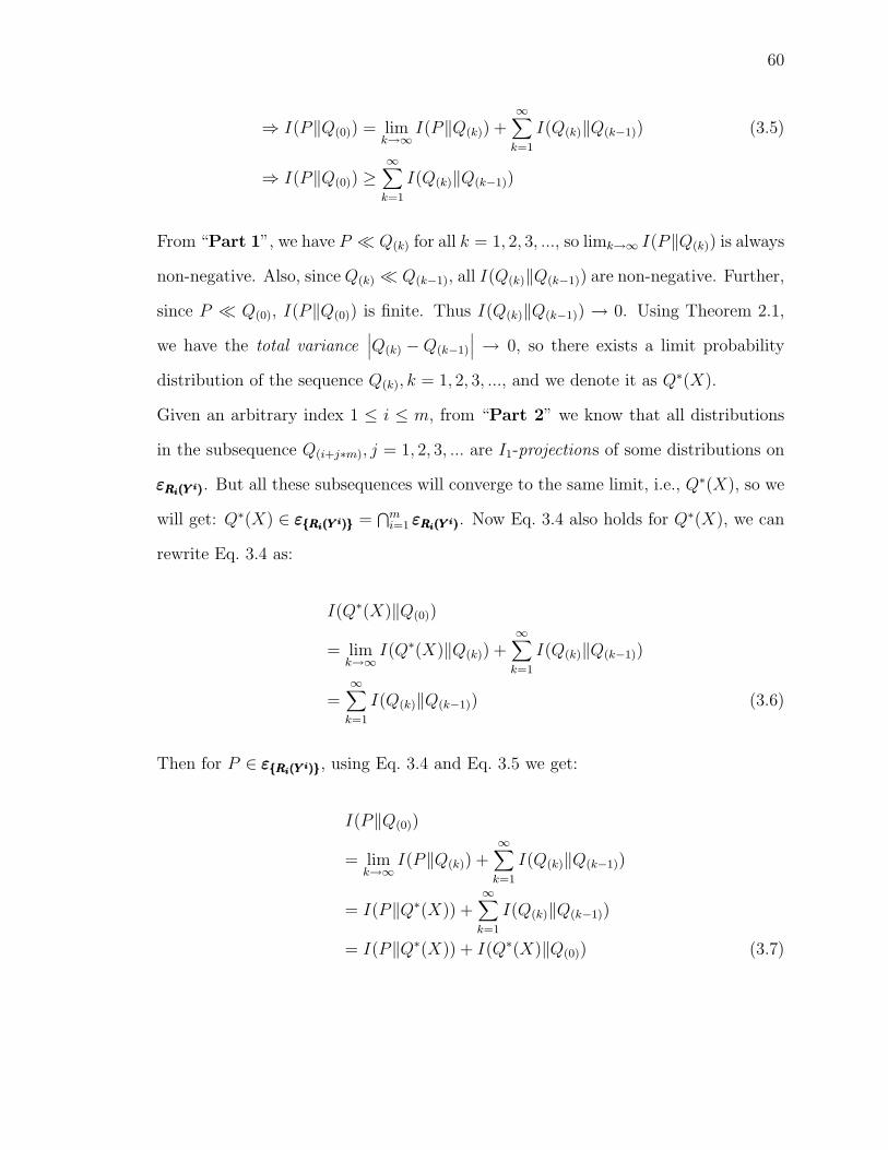
60
⇒ I(P‖Q(0)) = limk→∞
I(P‖Q(k)) +∞∑
k=1
I(Q(k)‖Q(k−1)) (3.5)
⇒ I(P‖Q(0)) ≥∞∑
k=1
I(Q(k)‖Q(k−1))
From “Part 1”, we have P ¿ Q(k) for all k = 1, 2, 3, ..., so limk→∞ I(P‖Q(k)) is always
non-negative. Also, since Q(k) ¿ Q(k−1), all I(Q(k)‖Q(k−1)) are non-negative. Further,
since P ¿ Q(0), I(P‖Q(0)) is finite. Thus I(Q(k)‖Q(k−1)) → 0. Using Theorem 2.1,
we have the total variance∣∣∣Q(k) −Q(k−1)
∣∣∣ → 0, so there exists a limit probability
distribution of the sequence Q(k), k = 1, 2, 3, ..., and we denote it as Q∗(X).
Given an arbitrary index 1 ≤ i ≤ m, from “Part 2” we know that all distributions
in the subsequence Q(i+j∗m), j = 1, 2, 3, ... are I1-projections of some distributions on
εRi(Y i)εRi(Y i)εRi(Y i). But all these subsequences will converge to the same limit, i.e., Q∗(X), so we
will get: Q∗(X) ∈ εRi(Y i)εRi(Y i)εRi(Y i) =⋂m
i=1 εRi(Y i)εRi(Y i)εRi(Y i). Now Eq. 3.4 also holds for Q∗(X), we can
rewrite Eq. 3.4 as:
I(Q∗(X)‖Q(0))
= limk→∞
I(Q∗(X)‖Q(k)) +∞∑
k=1
I(Q(k)‖Q(k−1))
=∞∑
k=1
I(Q(k)‖Q(k−1)) (3.6)
Then for P ∈ εRi(Y i)εRi(Y i)εRi(Y i), using Eq. 3.4 and Eq. 3.5 we get:
I(P‖Q(0))
= limk→∞
I(P‖Q(k)) +∞∑
k=1
I(Q(k)‖Q(k−1))
= I(P‖Q∗(X)) +∞∑
k=1
I(Q(k)‖Q(k−1))
= I(P‖Q∗(X)) + I(Q∗(X)‖Q(0)) (3.7)

61
Again, based on Eq. 2.4 of Theorem 2.2, Eq. 3.7 means Q∗(X) = πεRi(Yi)εRi(Yi)εRi(Yi)Q(0), that
finishes the whole convergence proof. 2
3.2 The Problem of Modifying BNs with Proba-
bilistic Constraints
Based on the notations, a network NNN0 on X = X1, ..., Xn has DAG GGG0 and CPT
set CCC0 where each CPT in CCC0 is in the form of P0(Xi|πi), and the JPD of NNN0 is
P0(X) =∏n
i=1 P0(Xi|πi).
Given a JPD P (X) and a BN structure GGG of X, a CPT P (Xi|πi) can be extracted
from P (X) by computing P (πi) and P (Xi, πi) from P (X) through marginalization or
any other methods. When P (X) and GGG are given, CPT extraction is unique. When
all CPTs of NNN are replaced by those extracted from an arbitrary P (X) according to
GGG, its distribution P ′(X) =∏n
i=1 P (Xi|πi) may not be equal to P (X) even though
the conditional distribution of Xi, given πi, are the same in both P (X) and P ′(X).
This is because certain conditional independences of P ′(X), dictated by the network
structure, do not hold for P (X).
A distribution P (X) is said to be (structurally) consistent with GGG of NNN if and
only if there exists a set of CPTs CCC = Q(Xi|πi) such that P (X) =∏n
i=1 Q(Xi|πi).
Since when GGG is given, P (X) uniquely determines P (Xi|πi) for all Xi, so if P (X)
is consistent with GGG then P (X) =∏n
i=1 P (Xi|πi). Consequently, if both P (X) and
P ′(X) are consistent with GGG, then P (X) = P ′(X) if and only if CCC = C′C′C′.
With the above notations, we can state precisely the problem we are trying to
solve as follows: for a given NNN over variables X with distribution Q(X) and a set of
consistent constraints R, find NNN∗ that meets the following three requirements:
1. GGG = GGG∗ (both networks have the same structure);

62
2. Q∗(X), the distribution of NNN∗, satisfies all constraints in R; and
3. I-divergence I(Q∗(X)‖Q(X)) is minimum among all distributions that meet
requirements 1 and 2.
For a given NNN0 and its distribution Q0(X) =∏n
i=1 Q0(Xi|πi) and constraint set
R, one can always obtain an I1-projection Q∗(X) of Q0(X) on R by IPFP (i.e.,
requirement 1 and 3). However, Q∗(X) is not guaranteed to be consistent with GGG0
(i.e., requirement 2). This is especially true if some constraints involve more than one
variables and they span over more than one CPT. This problem is illustrated in the
following examples with a small network NNN4 of four binary variables A,B, C, D, as
depicted in Fig. 3.2. In our context, “1” is used for a “True” state and “0” is used
for a “False” state.
Fig. 3.2: Network NNN4 of X = A,B, C, D and its CPTs

63
Fig. 3.3: Running IPFP with R1(B) and R2(C)
Fig. 3.4: Running IPFP with R3(A,D)

64
Fig. 3.3 gives Q∗(A,B,C,D), the JPD resulted from IPFP on NNN4 with two con-
straints R1(B) = (0.61, 0.39), R2(C) = (0.83, 0.17). I-divergence of Q∗ to the orig-
inal distribution is 0.5708. Also given are the CPTs of the four variables extracted
from Q∗ according to the network structure. We can verify that 1) Q∗(B) = R1(B)
and Q∗(C) = R2(C) (i.e., Q∗ satisfies both constraints), and 2) Q∗(A,B, C,D) =
Q∗(A) ·Q∗(B|A) ·Q∗(C|A) ·Q∗(D|B, C) (i.e., Q∗ is consistent with the network struc-
ture). Note here that CPTs of three nodes (A, B, C) have been changed.
However, it is different when a single constraint R3(A,D) = (0.1868, 0.2132,
0.1314, 0.4686) is applied. As can be seen from the left upper corner of Fig. 3.4,
the resulting distribution, although satisfying R3(A,D), is not consistent with the
structure of NNN4, i.e., Q∗(A,B, C,D) 6= Q∗(A) · Q∗(B|A) · Q∗(C|A) · Q∗(D|B, C).
We can modify the BN by extracting CPTs from Q∗(A,B,C,D) while keeping the
structure unchanged. The new CPTs and the JPD of the modified BN are given
in the right part of Fig. 3.4. It can be seen that, P (A,D), the joint distribution
computed from the modified BN with probabilities (0.1374, 0.2626, 0.1905, 0.4095),
is not equal to R3(A,D). This is because A and D are not within a single CPT and
the interdependency among variables has been altered by IPFP while attempting to
satisfy the constraint R3(A,D) and minimize I-divergence. I-divergence of the JPD
of the modified BN to the original distribution is 0.2611.
3.3 E-IPFP
To solve the BN modification problem defined in Section 3.2, we first extend IPFP
to handle the requirement that the solution distribution should be consistent with GGG0,
the structure of the given BN. Recall that whether a distribution Q(X) is consistent
with GGG0 can be determined by whether Q(X) =∏n
i=1 Q(Xi|πi), where the parent-child
relation in the right hand of the equation is determined by GGG0. We can thus treat
65
this requirement as a probabilistic constraint Rr(X) =∏n
i=1 Q(k−1)(Xi|πi) in IPFP.
Here Q(k−1)(Xi|πi) are extracted from Q(k−1)(X) according to GGG0. We call Rr(X) a
structural constraint.
Like any other constraint Ri(Yi), this constraint, when applied at step k of IPFP,
changes Q(k−1)(X) to Q(k)(X). By Eq. 2.6, Q(k)(X) = Rr(X) =∏n
i=1 Q(k−1)(Xi|πi),
thus meeting the structural consistency requirement.
Let Q0(X) =∏n
i=1 Q0(Xi|πi) be the distribution of a given network NNN0, and R be
the set of m given constraints. E-IPFP is a simple extension of IPFP by including
the structural constraint as the (m + 1)th constraint Rm+1(X). The algorithm E-
IPFP is stated in Table 3.1. Note that for convenience Step 2.2 skips the “zero”
case of Eq. 2.6 and Eq. 2.7. As a practical matter, convergence of E-IPFP can be
determined by testing if the difference between Q(k)(X) and Q(k−1)(X) (by any of a
number of metrics) is below a given threshold.
All constraints remain constant during the iteration process except Rm+1(X),
which changes its value every time it is applied. Nonetheless, as a distribution,
when Rm+1(X) is applied to Q(k−1)(X), the resulting Q(k)(X) = Rm+1(X) is an I1-
projection of Q(k−1)(X) on Rm+1(X). This is because Q(k)(X) is the only distribution
that satisfies Rm+1(X) since Rm+1(X) is a distribution of X, not of a subset of X. As
can be seen from [33, 152, 31] and Section 3.1, convergence of the original IPFP is a
consequence of the property that each iteration of IPFP produces an I1-projection of
the previous distribution on a constraint. Since this condition holds for our E-IPFP,
the process converges to a distribution Q∗(X), and Q∗(X) is an I1-projection of Q0(X)
on R1, R2, ..., Rm, Rm+1(X). Since Q∗(X) satisfies Rm+1(X), we have Q∗(X) =
∏ni=1 Q∗(Xi|πi), so it also satisfies the structural consistency requirement. Therefore,
among those distributions that satisfy given constraints in R and are consistent with
GGG0, Q∗(X) has the minimum I-divergence to Q0(X).
Application of E-IPFP to the network NNN4 of Fig. 3.2 with a single constraint

66
E-IPFP(NNN0(X), R = R1, R2, ..., Rm) 1. Computing Q0(X) =
∏ni=1 Q0(Xi|πi) where Q0(Xi|πi) ∈ CCC0;
2. Starting with k = 1, repeat the following procedure until convergence 2.1. i = ((k − 1) mod (m + 1)) + 1;
2.2. if i < m + 1 if (Ri ∈ Rm) /* for marginal constraints */
Q(k)(X) = Q(k−1)(X) · Ri(Yi)
Q(k−1)(Yi)
; (from Eq. 2.6)
else if (Ri ∈ Rc) /* for conditional constraints */
Q(k)(X) = Q(k−1)(X) · Ri(Yi|Zi)
Q(k−1)(Yi|Zi)
; (from Eq. 2.7)
2.3. else extract Q(k−1)(Xi|πi) from Q(k−1)(X) according to GGG0;
Q(k)(X) =∏n
i=1 Q(k−1)(Xi|πi);
2.4. k = k + 1;
3. return NNN
∗(X) with GGG∗ = GGG0 and CCC
∗ = Q(k)(Xi|πi);
Table 3.1: The E-IPFP Algorithm

67
Fig. 3.5: Running E-IPFP with R3(A,D)
R3(A,D) = (0.1868, 0.2132, 0.1314, 0.4686) converges to a distribution (Fig. 3.5).
Comparing with the result in Fig. 3.4 (using IPFP), this distribution not only satis-
fies R3(A,D), but is also structurally consistent with NNN4. However, its I-divergence to
the original distribution increases slightly in absolute value (from 0.2611 in Fig. 3.4
to 0.4419).
3.4 D-IPFP
As can be seen in Eq. 2.6 and Eq. 2.7, the computation of both IPFP and E-IPFP
is on the entire joint distribution of X at every iteration. This distribution becomes
prohibitively large with large n, making the process computationally intractable for
BNs of large size. Roughly speaking, when Q(k−1)(X) is modified by constraint Ri(Yi)
(or Ri(Yi|Zi)), Eq. 2.6 (or Eq. 2.7) requires to check each entry in Q(k−1)(X) against
every entry of Ri(Yi) (or Ri(Y
i|Zi)) and makes the update if x is consistent with yi

68
(or x is consistent with yi and zi). The cost can be roughly estimated as O(2n ∗ 2|Yi|)
(or O(2n ∗ 2|Yi|+|Zi|)), which grows exponentially with n.
Since the joint distribution of a BN is a product of distributions of much smaller
size (i.e., its CPTs), the cost of E-IPFP may be reduced if we can utilize the
interdependencies imposed on the distribution by the network structure and only
update some selected CPTs. This has motivated the development of algorithm D-
IPFP which decomposes the global E-IPFP (the one involving all n variables) into
a set of local E-IPFP, each for one constraint Ri(Yi) (or Ri(Y
i|Zi)), on a small
subnet of NNN0 that contains Y i (or Y i ∪ Zi).
Without loss of generality, now we assume all the constraints are from Rm. Con-
sider one such constraint Ri(Yi) at step k where Y i is a non-empty subset of X. Let
Y be some non-empty subset of X (i.e., Y ⊆ X and Y 6= ∅) such that Y i ⊆ Y ,
and let S = (⋃
Xj∈Y πj)\Y , i.e., S contains parent nodes of all variables in Y except
those that are also in Y . Multiplying all CPTs for variables in Y , one can construct
a conditional distribution Q′(k−1)(Y |S):
Q′(k−1)(Y |S) = Q(k−1)(Y |S) =
∏
Xj∈Y
Q(k−1)(Xj|πj) (3.8)
With Eq. 3.8, we can define Q′(k−1)(X) as follows:
Q′(k−1)(X) = Q(k−1)(X) = Q′
(k−1)(Y |S) · ∏
Xj /∈Y
Q(k−1)(Xj|πj) (3.9)
Now Ri(Yi) becomes local to the table Q′
(k−1)(Y |S), and we can obtain:
Q′(k)(X) = Q′
(k)(Y |S) · ∏
Xj /∈Y
Q(k)(Xj|πj)
by obtaining Q′(k)(Y |S) using Eq. 2.6 in the subspace of Y ∪ S while keeping CPTs

69
for variables outside Y unchanged:
Q′(k)(Y |S) = Q′
(k−1)(Y |S) · Ri(Yi)
Q′(k−1)
(Y i)· αk
Q′(k)(Xj|πj) = Q′
(k−1)(Xj|πj) = Q(k−1)(Xj|πj) for ∀Xj /∈ Y(3.10)
αk is a normalization vector. Next, we could extract Q′(k)(Xj|πj) for all Xj ∈ Y from
Q′(k)(Y |S), and let Q(k)(Xj|πj) = Q′
(k)(Xj|πj), then we can get Q(k)(X) by:
Q(k)(X) =∏
Xj∈Y
Q′(k)(Xj|πj)·
∏
Xj /∈Y
Q(k−1)(Xj|πj) (3.11)
Though Q′(k)(Y |S) satisfies Ri(Y
i), Q(k)(X) might not, so the process from Eq. 3.8
to Eq. 3.11 need to be repeated until converge. In summary, update of Q(k−1)(X)
to Q(k)(X) by Ri(Yi) can be seen to consist of iterations over three steps: 1) form
Q′(k−1)(Y |S) from CPTs for Xj ∈ Y by Eq. 3.8; 2) update Q′
(k−1)(Y |S) to Q′(k)(Y |S)
by Ri(Yi) using Eq. 3.10; and 3) extract Q′
(k)(Xj|πj) from Q′(k)(Y |S) and compute
the new distribution Q(k)(X) by Eq. 3.11. Comparing Eq. 3.8, Eq. 3.10 and Eq. 3.11
with Step 1, Step 2.2 and Step 2.3 in algorithm E-IPFP, this procedure of D-IPFP
for one constraint amounts to one application of the E-IPFP algorithm with two
constraints (i.e., Ri(Yi) and local structural constraint Rr(Y ) =
∏Xj∈Y
Q′(k)(Xj|πj))
on local distribution Q′(k−1)(Y |S) and it can be easily extended to handle constraints
from Rc. Then given a set of constraints R, the D-IPFP algorithm can be presented
as Table 3.2. For efficiency consideration, in implementing D-IPFP, the “while”
loop of Step 2.3 can be replaced by a single iteration.
Next we analyze the convergence of D-IPFP by first examining the behavior
involving a single constraint that iterates over Eq. 3.8 to Eq. 3.11 (i.e., Step 2.3 in
Table 3.2). This is given in Theorem 3.1 below.
Theorem 3.1 (Convergence of D-IPFP for One Constraint)

70
D-IPFP(NNN0(X), R = R1, R2, ..., Rm) 1. Computing Q0(X) =
∏ni=1 Q0(Xi|πi) where Q0(Xi|πi) ∈ CCC0;
2. Starting with k = 1, repeat the following procedure until convergence 2.1 i = ((k − 1) mod m) + 1;
2.2 getting the Y and S of this constraint, let counter kk = 0;
2.3 while not converge 2.3.1 Q′
(k−1)(Y |S) =∏
Xj∈YQ(k−1)(Xj|πj) ;
2.3.2 if (Ri ∈ Rm) /* for marginal constraints */
Q′(k)(Y |S) = Q′
(k−1)(Y |S) · Ri(Yi)
Q′(k−1)
(Y i)· αk;
else if (Ri ∈ Rc) /* for conditional constraints */
Q′(k)(Y |S) = Q′
(k−1)(Y |S) · Ri(Yi|Zi)
Q′(k−1)
(Y i|Zi)· αk;
2.3.3 Updating CPTs for all Xj ∈ Y and compiling the network;
Q(k)(Xj|πj) = Q′(k)(Xj|πj) ∀Xj ∈ Y
Q(k)(Xj|πj) = Q(k−1)(Xj|πj) ∀Xj /∈ Y
2.3.4 Q(k−1)(Xj|πj) = Q(k)(Xj|πj), for all Xj ∈ X ; kk = kk + 1 ;
2.4 k = k + 1;
3. return NNN
∗(X) with GGG∗ = GGG0 and CCC
∗ = Q(k)(Xi|πi);
Table 3.2: The D-IPFP Algorithm

71
Let Q(k−1)(X) =∏n
j=1 Q(k−1)(Xj|πj) be a probability distribution over variables X
where each Q(k−1)(Xj|πj) is the CPT for variable Xj in a Bayesian network NNN of n
variables. Let Ri(Yi) be a probability distribution over variables Y i ⊆ X that is
consistent with the structure of NNN. Then:
1. The iterations of Eq. 3.8 - Eq. 3.11 (i.e., Step 2.3 in Table 3.2), starting with
Q(k−1)(X), will converge to a distribution Q∗(k)(X);
2. Q∗(k)(X) satisfies Ri(Y
i), i.e., Q∗(k)(Y
i) = Ri(Yi);
3. Q∗(k)(X) is consistent with the structure of NNN;
4. Q∗(k)(X) is not always the I1-projection of Q(k−1)(X) on Ri(Y
i), but on con-
straint set Ri(Yi), Rr(Y ).
Proof.
Part 1. Note that Eq. 3.8 and Eq. 3.9 do not change the distribution, they only change
its representation. Eq. 3.11 imposes a local structural constraint on Q′(k−1)(Y |S), as
argued in Section 3.3 for E-IPFP, Q(k)(Y |S) is thus an I1-projection of Q′(k)(Y |S)
on Rr(Y ), i.e., Q(k)(X) is thus an I1-projection of Q′(k)(X) on Rr(Y ) since all other
CPTs are unchanged. Now we show that, with Eq. 3.10, Q′(k)(X) is an I1-projection
of Q′(k−1)(X). Combining Eq. 3.8, Eq. 3.9, and Eq. 3.10, we have
Q′(k)(X) = Q′
(k)(Y |S) · ∏
Xj /∈Y
Q′(k−1)(Xj|πj)
= [Q′(k−1)(Y |S) · ∏
Xj /∈Y
Q′(k−1)(Xj|πj)] ·
Q′(k)(Y |S)
Q′(k−1)(Y |S)
= Q′(k−1)(X) · Q′
(k)(Y |S)
Q′(k−1)(Y |S)
Therefore, Q′(k)(X) is an I1-projection of Q′
(k−1)(X) on constraint Q′(k)(Y |S). Since
each update generates a distribution that is an I1-projection of the previous distri-

72
bution, again, according to [33, 152, 31] and Section 3.1, the process converges with
limkk→∞ Q(k)(x) = Q∗(k)(X). Note that kk is the counter for Step 2.3 which accumu-
lates the number of iterations for the internal “while” loop in Table 3.2.
Part 2. We prove this part by showing that when kk →∞, Ri(Yi)
Q′(k−1)
(Y i)→ 1. Note,
Q′(k−1)(Y |S) · Ri(Y
i)
Q′(k−1)(Y
i)
= Q′(k−1)(Y |S) · Q′
(k−1)(S)
Q′(k−1)(S)
· Ri(Yi)
Q′(k−1)(Y
i)
=Q′
(k−1)(Y, S)
Q′(k−1)(S)
· Ri(Yi)
Q′(k−1)(Y
i)
=Q′
(k)(Y, S)
Q′(k−1)(S)
= Q′(k)(Y |S) · Q′
(k)(S)
Q′(k−1)(S)
(3.12)
By Part 1, when kk → ∞, Q′(k)(X) − Q′
(k−1)(X) → 0. Then we haveQ′
(k)(S)
Q′(k−1)
(S)→ 1
andQ′
(k)(Y |S)
Q′(k−1)
(Y |S)→ 1. Substituting these limits into Eq. 3.12, we have Ri(Y
i)Q′
(k−1)(Y i)
→ 1.
Part 3. This is to show Q(k)(X) =∏
Xi∈XQ(k)(Xi|πi). Similarly, by Part 1, when
kk → ∞, Q(k)(X) − Q′(k)(X) → 0. Since
∏Xj /∈Y
Q(k−1)(Xj|πj) has never changed, it
can be factored out. Then according to Eq. 3.10 and Eq. 3.11, we have:
Q(k)(Y |S)−Q′(k)(Y |S) =
∏
Xj∈Y
Q′(k)(Xj|πj)−Q′
(k)(Y |S) → 0
Thus Q′(k)(Y |S) is consistent with the network structure with variables in Y . Since
other CPT’s have not been changed, Q∗(k)(X) is still consistent with the network
structure of NNN.
Part 4. We prove it by a counter example. In the example in Fig. 3.4 at the end of
Section 1, an I1-projection on R3(A,D) is not consistent with the network structure.

73
On the other hand, Q∗(k)(X) from D-IPFP must be consistent with the network
structure. Since I1-projection is unique, Q∗(k)(X) therefore cannot be an I1-projection
of Q(k−1)(X) on Ri(Yi) only. Actually, as proved earlier 3, Q∗
(k)(X) is an I1-projection
of Q(k−1)(X) on constraint set Ri(Yi), Rr(Y ). 2
Theorem 3.1 can be easily extended to the case of conditional constraints. When
D-IPFP is applied to a set of constraints, according to Theorem 3.1, each iteration of
D-IPFP for one constraint produces an I1-projection of the previous distribution on
a constraint set Ri(Yi), Rr(Y ), so, similar to “Part 3” of the IPFP convergence
proof in Section 3.1, the complete D-IPFP process converges to a distribution
Q∗(X) which is an I1-projection of Q0(X) on R∪∀Rr(Y )∪Rr(X). Rr(X) is also
satisfied since in each iteration all other CPTs not related to Y will be unchanged.
Compare this result to that of E-IPFP, the I-divergence I(Q∗(X)‖Q0(X)) of D-
IPFP will be slightly larger than that of E-IPFP, since D-IPFP satisfies on more
constraints. There is a trade off between accuracy and efficiency when choosing which
algorithm to use.
Now the remaining problem is how to get a good Y from Y i?
(Y1) The extreme case is to let Y = X, and thus S = ∅, which reduces the
D-IPFP process to E-IPFP, or we could say that E-IPFP is a special case of
D-IPFP with Y = X.
(Y2) A simplest case is to let Y = Y i (or Y = Y i∪Zi for conditional constraint).
In this case, it is possible that some Xi ∈ S, which is the parent of Xt ∈ Y i, is also a
child of some Xj ∈ Y i. Based on the BN independence assumption, if the CPT of Xi
is also allowed to be changed, the resulting distribution will have smaller I-divergence
to the original distribution than that of (Y2) and this I-divergence will be very close
to that of E-IPFP , thus brings out the third method to get Y .
3As stated earlier, this D-IPFP for one constraint Ri(Y i) amounts to one application of a localE-IPFP, so the convergence result of E-IPFP in Section 3.3 can be applied to here directly.

74
(Y3) Originally, Y = Y i (or Y = Y i ∪ Zi for conditional constraint) and S =
(⋃
Xj∈Y i πj)\Y i, then repeat the following process until nothing more could be added
to Y : if Xi ∈ S and Xj ∈ Y i and Xj ∈ πi, then Y = Y ∪Xi, S = (S−Xi)∪(πi\Y ).
Fig. 3.6: Running D-IPFP(Y2) with R3(A,D)
Consider again the network NNN4 in Fig. 3.2 with a single non-local constraint
R3(A,D), if we have Y = A,D and S = B, C by (Y2), the new table
Q′(A, D|B, C) can be computed as the product of Q(A) and Q(D|B, C) of the orig-
inal BN. For example, one entry of this table Q′(A = 1, D = 0|B = 1, C = 1) is
0.4 ∗ 0.9 = 0.36. Then we applied D-IPFP to the BN in Fig. 3.2 with the non-local
constraint R3(A,D). The process converged. The resulting BN satisfies the constraint
R3(A,D), and only CPT for D has been changed (See Fig. 3.6, note that the CPT
for A is not changed in this case but it is possible to be changed in other cases, but
the CPTs for B and C will never be changed.). As expected, the I-divergence with
D-IPFP was worse than that with E-IPFP (increased from 0.4419 to 0.7815).
The moderate sacrifice in I-divergence with D-IPFP is rewarded by a signifi-

75
cant saving in computation. Since Ri(Yi) is now used to modify Q′
(k−1)(Y |S), not
Qk−1(X), the cost for each step is reduced from O(2n ∗ 2|Y i|) to O(2|S|+|Y | ∗ 2|Y i|),where O(2|S|+|Y |) is the size of CPT Q′
(k−1)(Y |S). The saving is thus in the order of
O(2n−|S|−|Y |).
3.5 SD-IPFP
A probabilistic constraint is local if it contains only one variable and some of its
parents, i.e., Ri(Yi) = Ri(Xj, Z
j ⊆ πj) for marginal constraint or Ri(Yi|Zi) =
Ri(Xj|Zj ⊆ πj) for conditional constraint. In either case, when applying D-IPFP
to the constraint, Y = Xj, S = πj, and Step 2.3 in Table 3.2 can be replaced by
one step:
Q(k)(Xj|πj) = Q(k−1)(Xj|πj) · Ri(Yi)
Q(k−1)(Yi)· αk
Q(k)(Xl|πl) = Q(k−1)(Xl|πl) for l 6= j(3.13)
for marginal constraint Ri(Yi), where
αk =∑xj
Q(k−1)(xj|πj)Ri(y
i)
Q(k−1)(yi)
αk is the normalization factor. Similar equations can be obtained in case of conditional
constraint. Since only the table for Xj is changed, Eq. 3.11 is rewritten to:
Q(k)(X) = Q(k)(Xj|πj) ·∏
l 6=j
Q(k−1)(Xl|πl) (3.14)
Therefore Q(k)(X) is consistent with G0, i.e., it satisfies the structural constraint.
Eq. 3.14 can also be written as:
Q(k)(X)
= Q(k−1)(Xj|πj) · Ri(Yi)
Q(k−1)(Y i)· αk ·
∏
l 6=j
Q(k−1)(Xl|πl)
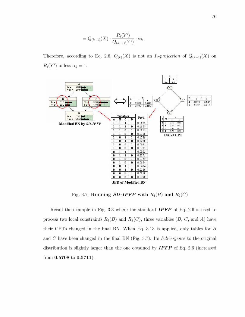
76
= Q(k−1)(X) · Ri(Yi)
Q(k−1)(Y i)· αk
Therefore, according to Eq. 2.6, Q(k)(X) is not an I1-projection of Q(k−1)(X) on
Ri(Yi) unless αk = 1.
Fig. 3.7: Running SD-IPFP with R1(B) and R2(C)
Recall the example in Fig. 3.3 where the standard IPFP of Eq. 2.6 is used to
process two local constraints R1(B) and R2(C), three variables (B, C, and A) have
their CPTs changed in the final BN. When Eq. 3.13 is applied, only tables for B
and C have been changed in the final BN (Fig. 3.7). Its I-divergence to the original
distribution is slightly larger than the one obtained by IPFP of Eq. 2.6 (increased
from 0.5708 to 0.5711).

77
3.6 The IPFP API
Surprisingly, one can not find any available code about IPFP, which motivated me to
implement an API for all the variants of IPFP algorithms, as discussed in previous
sections. It is organized into three packages: “DiscreteProb” which includes classes
and methods for storing and updating probability distributions, “GenericIPFP” which
includes the implementations of the existing IPFP and C-IPFP algorithms, and
“ExtendedIPFP” which includes the implementations of the extended E-IPFP, D-
IPFP, SD-IPFP algorithms, as well as methods (included in the “Transform”
module) used for extracting CPTs for a BN DAG from given JPD and methods used
for obtaining MPDs for a set of variables from a given BN. The class diagram is shown
in Fig. 3.8, the dashed arrow indicates the dependency between packages.
Fig. 3.8: Class Diagram of the IPFP API
There are many existing software packages for Bayesian networks that are written
in various languages and provide different features in reasoning and learning. Inter-
ested readers may refer to http://www.cs.ubc.ca/~murphyk/Bayes/bnsoft.html
for a complete list of packages and a tabular comparison among them, which is main-
tained by Kevin Murphy 4 in University of British Columbia, Canada. In my imple-
4http://www.cs.ubc.ca/~murphyk/

78
mentation, I used the NeticaJ API purchased from Norsys 5. NeticaJ is implemented
in Java and provided with complete Javadocs. It is powerful and easy to use. It
can do belief updating using junction trees, parameter learning from case files, spec-
ifies findings to variables, and provides a graphic representation of the network. The
classes and methods implemented in the “Transform” module are based on this API.
The realization of the different variants of IPFP algorithms depends on the suc-
cessful implementation of the “DiscreteProb” module and the “Transform” module.
While the latter can be easily implemented using the NeticaJ API, the former need
to be dealt with great care. The core component of the “DiscreteProb” module is
the simulation of a dynamic multi-dimensional array which is used to hold probabil-
ity values. Classes for random variables and probability distributions are built upon
this multi-dimensional array. A random variable has a name and a set of states. A
JPD has a set of random variables, and an corresponding multi-dimensional array for
probability values. A CPD has a set of prior random variables, a set of condition ran-
dom variables, and an corresponding multi-dimensional array for probability values.
Methods for JPD marginalization and for computation of distance measures between
two JPDs such as I-divergence and total variance are also provided. The various
IPFP algorithms are then implemented based on these methods. The experimental
results shown in next section are obtained using this API.
3.7 Experiments
First, as shown in Fig. 3.9, a comparison is made among E-IPFP, D-IPFP(Y2),
and D-IPFP(Y3) for modifying NNN4 in Fig. 3.2 with the constraint sets R3(A,D)and R(B), R(C), respectively, when using the same stop criteria (i.e., when the
total variance between JPDs obtained from two consecutive iterations is smaller than
0.0001). E-IPFP always has the minimal total variance and I-divergence, as proved
5http://www.norsys.com/
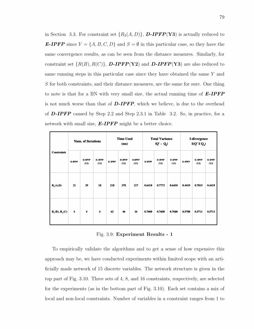
79
in Section 3.3. For constraint set R3(A,D), D-IPFP(Y3) is actually reduced to
E-IPFP since Y = A,B,C, D and S = ∅ in this particular case, so they have the
same convergence results, as can be seen from the distance measures. Similarly, for
constraint set R(B), R(C), D-IPFP(Y2) and D-IPFP(Y3) are also reduced to
same running steps in this particular case since they have obtained the same Y and
S for both constraints, and their distance measures, are the same for sure. One thing
to note is that for a BN with very small size, the actual running time of E-IPFP
is not much worse than that of D-IPFP, which we believe, is due to the overhead
of D-IPFP caused by Step 2.2 and Step 2.3.1 in Table 3.2. So, in practice, for a
network with small size, E-IPFP might be a better choice.
0.5708
0.4419
E - IPFP
I - divergence
I(Q * || Q 0 )
0.5711
0.7815
D - IPFP
(Y2)
0.5711 0.7600 0.7600 0.7600 16 46 62 4 4 4 R 1 (B), R
2 (C)
0.4419 0.6410 0.7772 0.6410 217 378 218 10 29 21 R 3 (A,D)
D - IPFP
(Y3)
D - IPFP
(Y3)
D - IPFP
(Y2) E - IPFP
D - IPFP
(Y3)
D - IPFP
(Y2) E - IPFP
D - IPFP
(Y3)
D - IPFP
(Y2) E - IPFP
Total Variance
|Q * - Q 0 |
Time Used
(ms) Num. of Iterations
Constraints
Fig. 3.9: Experiment Results - 1
To empirically validate the algorithms and to get a sense of how expensive this
approach may be, we have conducted experiments within limited scope with an arti-
ficially made network of 15 discrete variables. The network structure is given in the
top part of Fig. 3.10. Three sets of 4, 8, and 16 constraints, respectively, are selected
for the experiments (as in the bottom part of Fig. 3.10). Each set contains a mix of
local and non-local constraints. Number of variables in a constraint ranges from 1 to

80
Fig. 3.10: A Network of 15 Variables
3, the size of the subnet associated with a constraint (|Y | + |S|) ranges from 2 to 6.
Therefore a saving in computational time would be in the order of O(215−6) = O(29)
if not including the overhead caused by Step 2.2 and Step 2.3.1 in Table 3.2. Both
E-IPFP, D-IPFP(Y2), and D-IPFP(Y3) were run for each of the three sets
using the same stop criteria (i.e., when the total variance between JPDs obtained
from two consecutive iterations is smaller than 0.005). The program is a brute force
implementation of the two algorithms without any optimization. The experiments
were run on a DELL OPTIPLEX GX270 Intel Pentium 4 Desktop of 2.4GHz CPU,
1GB RAM, and 784M maximum memory for the JVM (Java Virtual Machine). The

81
results are reported in Fig. 3.11.
0.5665 0.6292 0.5618 0.6226 0.6694 0.6192 15 107 581 4 9 8 8
2.5284
0.0811
E - IPFP
I - divergence
I(Q * || Q 0 )
2.6146
0.3401
D - IPFP
(Y2)
2.5321 1.2593 1.2595 1.2579 189 45 769 5 7 9 16
0.0826 0.2785 0.4113 0.2757 0.406 0.75 533 7 3 8 4
D - IPFP
(Y3)
D - IPFP
(Y3)
D - IPFP
(Y2) E - IPFP
D - IPFP
(Y3)
D - IPFP
(Y2) E - IPFP
D - IPFP
(Y3)
D - IPFP
(Y2) E - IPFP
Total Variance
|Q * - Q 0 |
Time Used
(seconds) Num. of Iterations
Num. of
Constraints
Fig. 3.11: Experiment Results - 2
Each of the 9 experimental runs converged to a distribution that satisfies all given
constraints and is consistent with the network structure. As expected, D-IPFP
is significantly faster than E-IPFP but with moderately larger I-divergences when
using (Y2) to get the Y and S in the algorithm. Also, from both Fig. 3.9 and Fig. 3.11
we can see that in general E-IPFP has smaller I-divergences, then D-IPFP(Y3),
and finally D-IPFP(Y2). This is consistent with our theoretical analysis. The rate
of speed up of D-IPFP is roughly in the theoretically estimated range (O(29)) for the
case of 4 constraints, when the overhead is small. For the case of 8 and 16 constraints,
the overhead used to find Y and S and extract local distributions Q′(k−1)(Y |S) from
BN for each of the constraints in each iteration become significant with a network of
size 15. However, D-IPFP is still much faster than E-IPFP.

82
3.8 Summary
In this chapter, we developed algorithm E-IPFP that extends IPFP to modify
probability distributions represented as Bayesian networks. The modification is done
by only changing the conditional probability tables of the network while leaving the
network structure intact. We also show a significant saving in computational cost
can be achieved by decomposing the global E-IPFP into local ones with a much
smaller scale, as described in algorithm D-IPFP. Computer experiments within lim-
ited scope seem to validate the analysis results. These algorithms can be valuable tools
in Bayesian network construction, merging and refinement when low-dimensional dis-
tributions need to be incorporated into the network. D-IPFP can be simplified and
rewritten to SD-IPFP when only dealing with local constraints (priors or pair-wise
marginals), which will be further extended in BayesOWL for CPT construction
under the condition of a given set of hard evidences.
Several pieces of existing work are particularly relevant to this work, besides those
related to the development of the original IPFP and proofs of its convergence. Diaco-
nis and Zabell (1982) [37], in studying the role of Jeffrey’s rule in updating subjective
probability, consider IPFP as one of methods for mechanical updating of probability
distribution. In contrast to other methods that are based on different assumptions
on the subjectivity of the probabilities, the mechanical updating methods are based
on some distance metrics, rather than “attempt to quantify one’s new degree of belief
via introspection”.
Vomlel (1999) [152] studied in detail how IPFP can be used for probabilistic
knowledge integration in which a joint probability distribution (the knowledge base)
is built from a set of low dimensional distributions, each of which models a sub-
domain of the problem. Besides providing a cleaner, more readable convergence
proof for IPFP, he also studied the behavior of IPFP with input set generated by
decomposable generating class. If such input distributions can be properly ordered,

83
IPFP may converge in one or two cycles. This kind of input set roughly corresponds
to ordering constraints for a Bayesian network in such a way that the constraint
involving ancestors are applied before those involving descendants, if such order can
be determined. For example, if all three constraints R1(B), R2(C), R3(A, D) must
be met, we may be better off by applying R3(A,D) before the other two.
In all of these works, IPFP is applied to update joint distributions, none has
discussed its application in modifying distributions represented by a BN.
To the best of our knowledge, the only work that applies IPFP to BN is the one
by Valtorta et al (2000) [147]. In this work, IPFP is used to support belief update
in BN by a set of soft evidences that are observed simultaneously. However, this work
does not concern itself with updating the BN itself.
Algorithms developed in this chapter only work with consistent constraints. What
will happen when the given probabilistic constraints are not consistent with each
other? A number of computational experiments [152, 153] show that IPFP will
either fail to find a distribution because of the violation of “dominance” or the
Q(k), k = 1, 2, 3, ... sequence will oscillate in cycles and never converge. How to han-
dle inconsistent constraint is one of the important directions for future research. In
Vomlel’s thesis [152], he presents two basic approaches in solving this problem. The
first is to define some “distance measure” from the marginals of a distribution in
the oscillating sequence to the given constraints, and choose the one that minimizes
the distance measure as the best solution of running IPFP, however, this approach
does not work in the case of “fails”. The second approach, referred as “missing data
methods”, aims to modify the given inconsistent probabilistic constraints to make it
workable for IPFP, and is based on the assumption that the given probabilistic con-
straints are estimated as relative frequencies from data and the inconsistency comes
from incomplete, incorrect, or missing data. In this case, methods from Statistics can
be borrowed to analysis and process the inconsistent data.

84
Another direction is to investigate in what situations modification of only con-
ditional probability tables is no longer sufficient or desirable, the network structure
need also be changed in order to better satisfy given constraints.
Efficiency of this approach also needs serious investigation. As our experiments
show, EIPFP in general is very expensive. The convergence time in our experiments
with a small BN (15 nodes) and moderate number of constraints is in the order of tens
of minutes when the stop criteria is low or hours when the stop criteria is high. The
performance of even D-IPFP can be worse if some input distributions involve larger
number of variables. Complexity can be reduced if we can divide a large constraint
into smaller ones by exploring independence between the variables (possibly based on
the network structure). Properly ordering the constraints may also help. Ultimately,
this problem can only be solved by parallelizing the algorithms or by approximation
when the network is really large.

Chapter 4
BayesOWL - A Probabilistic Extension to
OWL
This chapter presents BayesOWL in detail. As mentioned earlier, BayesOWL is
a framework which augments and supplements the semantic web ontology language
OWL 1 for representing and reasoning with uncertainty based on Bayesian networks
(BN) [121]. BayesOWL provides a set of rules and procedures for direct translation
of an OWL taxonomy ontology into a BN directed acyclic graph (DAG), it also
provides a method based on iterative proportional fitting procedure (IPFP)
[79, 36, 33, 152, 18, 31] that incorporates available probabilistic constraints when
constructing the conditional probability tables (CPTs) of the translated BN. The
translated BN, which preserves the semantics of the original taxonomy ontology and is
consistent with all the given probabilistic constraints, can support ontology reasoning,
both within and across ontologies as Bayesian inferences. If two taxonomy ontologies
are translated to two BNs, then concept mapping between these taxonomy ontologies
can be accomplished by evidential reasoning across the translated BNs. Discussion
and some preliminary works on this issue will be presented at the end of Chapter 5.
This chapter is organized as follows: Section 4.1 proposes a representation in
OWL of probabilistic information concerning the entities and relations in ontologies
which will be used as constraints to construct CPTs of the translated BN; Section
4.2 presents the structural translation rules; Section 4.3 presents the method used for
CPT construction; Section 4.4 presents the semantics of BayesOWL; Section 4.5
talks about the possible reasoning tasks. Section 4.6 describes the OWL2BN API
1http://www.w3.org/2001/sw/WebOnt/
85

86
for structural translation, which, together with the IPFP API described in Section
3.6, builds up an initial version of the BayesOWL framework. An example that
translates an OWL taxonomy ontology of over 70 defined concepts into a BN DAG is
presented. Section 4.7 compares BayesOWL to other related works. The chapter
ends with discussion and suggestions for future research in Section 4.8.
4.1 Representing Probabilistic Information
Information about the uncertainty of the classes and relations in an ontology can
often be represented as probability distributions (e.g., P (C) and P (C|D)), which we
refer to as probabilistic constraints on the ontology. These probabilities can be either
provided by domain experts or learned from data.
The model-theoretic semantics 2 of OWL treats the domain as a non-empty col-
lection of individuals. If class A represents a concept, we treat it as a random binary
variable of two states a and a, and interpret P (A = a) as the prior probability or
one’s belief that an arbitrary individual belongs to class A, and P (a|b) as the condi-
tional probability that an individual of class B also belongs to class A. Similarly, we
can interpret P (a), P (a|b), P (a|b), P (a|b) and with the negation interpreted as “not
belonging to”.
Although not necessary, it is beneficial to represent the probabilistic constraints
as OWL statements. We have developed such a representation. Currently, our trans-
lation framework only allows to encode two types of probabilities into the original
ontology:
1. prior or marginal probability P (C);
2. conditional probability P (C|OC) where OC ⊆ πC , πC 6= ∅, OC 6= ∅.for a concept class C and its parent superconcept class set πC . This is because they
correspond naturally to classes and relations (RDF triples) in an ontology, and are
2http://www.w3.org/TR/owl-semantics/direct.html

87
most likely to be available to ontology designers. The representation can be easily
extended to constraints of other more general forms if needed.
We treat a probability as a kind of resource, and define two OWL classes: “Prior-
Prob”, “CondProb”. A prior probability P (C) of a variable C is defined as an instance
of class “PriorProb”, which has two mandatory properties: “hasVarible” (only one)
and “hasProbValue” (only one). A conditional probability P (C|OC) of a variable C
is defined as an instance of class “CondProb” with three mandatory properties: “has-
Condition” (at least has one), “hasVariable” (only one), and “hasProbValue” (only
one). The range of properties “hasCondition” and “hasVariable” is a defined class
named “Variable”, which has two mandatory properties: “hasClass” and “hasState”.
“hasClass” points to the concept class this probability is about and “hasState” gives
the “True” (belong to) or “False” (not belong to) state of this probability. The defined
ontology “prob.owl” is attached in “Appendix”.
<Variable rdf:ID=“c”>
<hasClass>C</hasClass>
<hasState>True</hasState>
</Variable>
<PriorProb rdf:ID=“P(c)”>
<hasVariable>c</hasVariable>
<hasProbValue>0.8</hasProbValue>
</PriorProb>
Table 4.1: Representing P (c) = 0.8 in OWL
For example, P (c) = 0.8, the prior probability that an arbitrary individual belongs
to class C, can be expressed as Table 4.1 and P (c|p1, p2, p3) = 0.8, the conditional
probability that an individual of the intersection class of P1, P2, and P3 also belongs
to class C, can be expressed as Table 4.2. For simplicity we did not consider the

88
namespaces in these examples.
<Variable rdf:ID=“c”> <Variable rdf:ID=“p3”>
<hasClass>C</hasClass> <hasClass>P3</hasClass>
<hasState>True</hasState> <hasState>True</hasState>
</Variable> </Variable>
<Variable rdf:ID=“p1”> <CondProb rdf:ID=“P(c|p1, p2, p3)”>
<hasClass>P1</hasClass> <hasCondition>p1</hasCondition>
<hasState>True</hasState> <hasCondition>p2</hasCondition>
</Variable> <hasCondition>p3</hasCondition>
<Variable rdf:ID=“p2”> <hasVariable>c</hasVariable>
<hasClass>P2</hasClass> <hasProbValue>0.8</hasProbValue>
<hasState>True</hasState> </CondProb>
</Variable>
Table 4.2: Representing P (c|p1, p2, p3) = 0.8 in OWL
4.2 Structural Translation
At the present time, BayesOWL is restricted to translating only OWL-DL concept
taxonomies into BNs. This section focuses on the translation of an OWL taxonomy
ontology into the network structure, i.e., the DAG of a BN. The task of construct-
ing CPTs will be considered in the next section. For simplicity, constructors for
header components in the ontology, such as “owl:imports” (for convenience, assume
an ontology involves only one single OWL file), “owl:versionInfo”, “owl:priorVersion”,
“owl:backwardCompatibleWith”, and “owl:incompatibleWith” are ignored since they
are irrelevant to the concept definition. Since the domain of discourse is treated as
a non-empty collection of individuals (“owl:Thing”), then every concept class (ei-
ther primitive or defined) can be thought as a countable subset (or subclass) of

89
“owl:Thing”.
In the semantic web, an important component of an ontology defined in OWL
or RDF(S) is the taxonomical concept subsumption hierarchy based on class axioms
and logical relations among the concept classes. At the present time, we focus our
attention to OWL ontologies defined using only constructors in these two categories
(as in Table. 4.3). Constructors related to properties, individuals, and datatypes will
be considered in the future.
Constructor DL Syntax Class Axiom Logical Operator
rdfs:subClassOf C1 v C2 *
owl:equivalentClass C1 ≡ C2 *
owl:disjointWith C1 v ¬C2 and C2 v ¬C1 *
owl:unionOf C ≡ C1 t ... t Cn *
owl:intersectionOf C ≡ C1 u ... u Cn *
owl:complementOf ¬C *
Table 4.3: Supported Constructors
Conversion of an OWL concept taxonomy into a BN DAG is done by a set of struc-
tural translation rules. The general principle underlying these rules is that all classes
(specified as “subjects” and “objects” in RDF triples of the OWL file) are translated
into nodes (named concept nodes) in BN, and an arc is drawn between two concept
nodes in BN only if the corresponding two classes are related by a “predicate” in
the OWL file, with the direction from the superclass to the subclass. A special kind
of nodes (named L-Nodes) are created during the translation to facilitate modeling
relations among concept nodes that are specified by OWL logical operators. These
structural translation rules are summarized as follows:
1. Every primitive or defined concept class C is mapped into a binary variable
node in the translated BN. Node C in the BN can be either “True” or “False”,

90
represented as c or c, indicating whether a given instance o belongs to concept
C or not.
2. Constructor “rdfs:subClassOf” is modeled by a directed arc from the parent
superclass node to the child subclass node. For example, a concept class C de-
fined with superconcept classes Ci(i = 1, ..., n) by “rdfs:subClassOf” is mapped
into a subnet in the translated BN with one converging connection from each
Ci to C, as illustrated in (Fig. 4.1).
Fig. 4.1: “rdfs:subClassOf”
3. A concept class C defined as the intersection of concept classes Ci(i = 1, ..., n),
using constructor “owl:intersectionOf” is mapped into a subnet (Fig. 4.2) in
the translated BN with one converging connection from each Ci to C, and one
converging connection from C and each Ci to an L-Node called “LNodeInter-
section”.
Fig. 4.2: “owl:intersectionOf”

91
4. A concept class C defined as the union of concept classes Ci(i = 1, ..., n), using
constructor “owl:unionOf” is mapped into a subnet (Fig. 4.3) in the translated
BN with one converging connection from C to each Ci , and one converging
connection from C and each Ci to an L-Node called “LNodeUnion”.
Fig. 4.3: “owl:unionOf”
5. If two concept classes C1 and C2 are related by constructors “owl:complementOf”,
“owl:equivalentClass”, or “owl:disjointWith”, then an L-Node (named “LN-
odeComplement”, “LNodeEquivalent”, “LNodeDisjoint” respectively, as in Fig. 4.4)
is added to the translated BN, and there are directed links from C1 and C2 to
the corresponding L-Node.
Fig. 4.4: “owl:complementOf, owl:equivalentClass, owl:disjointWith”
Based on rules 1 to 5, the translated BN contains two kinds of nodes: concept
nodes for regular concept classes and L-Nodes which bridge concept nodes that are
associated by logical relations. L-nodes are leaf nodes, with only in-arcs. With
all logical relations, except “rdfs:subClassOf”, handled by L-nodes, the in-arcs to a

92
concept node can only come from its parent superclass nodes. This makes C’s CPT
smaller and easier to construct. L-nodes also help avoid forming cycles in translated
BN. Since L-nodes are leaves, no cycles can be formed with L-nodes. The only place
where cycles can be defined for OWL taxonomies is by ”rdf:subClassOf” (e.g., A is
a subclass of B and B is a subclass of A). However, according to OWL semantics,
all concepts involved in such a ‘subclass’ cycle are equivalent to each other. We can
always detect this type of cycles in the pre-processing step and use rule 5, instead of
rule 2, to handle the translation.
In the translated BN, all arcs are directed based on OWL statements, two concept
nodes without any defined or derived relations are d-separated with each other, and
two implicitly dependent concept nodes are d-connected with each other but there
is no arc between them. Note that, this translation process may impose additional
conditional independence to the nodes by the d-separation in the BN structure [121].
For example, consider nodes B and C, which are otherwise not related except that
they both are subclasses of A. Then in the translated BN, B is conditionally inde-
pendent of C, given A. Such independence can be viewed as a default relationship,
which holds unless information to the contrary is provided. If dependency exists, it
can be modeled by using additional nodes similar to the L-Nodes.
4.3 CPT Construction
To complete the translation the remaining issue is to assign a conditional probability
table (CPT) P (C|πC) to each variable node C in the DAG, where πC is the set of
all parent nodes of C. As described earlier, the set of all nodes X in the translated
BN can be partitioned into two disjoint subsets: concept nodes XC which denote
concept classes, and L-Nodes XL for bridging concept nodes that are associated by
logical relations. In theory, the uncertainty information about concept nodes and

93
their relations may be available in probability distributions of any arbitrary forms, our
observation, however, is that it is most likely to be available from the domain experts
or statistics in the forms of prior probabilities of concepts and pair-wise conditional
probabilities of concepts, given a defined superclass. Therefore, the method developed
in this section accommodates two types of probabilities with respect to a concept node
C ∈ XC : prior probability P (C), and conditional probability P (C|OC ⊆ πC) where
OC 6= ∅, as mentioned earlier in Section 4.1. Methods for utilizing probabilities in
arbitrary forms and dimensions [123] is reported in Chapter 3. Before going into the
details of constructing CPTs for concept nodes in XC based on available probabilistic
information, CPTs for the L-Nodes in XL are discussed first.
CPTs for L-Nodes
CPT for an L-Node can be determined by the logical relation it represents so that
when its state is “True”, the corresponding logical relation holds among its par-
ents. Based on the structural translation rules, there are five types of L-Nodes corre-
sponding to the five logic operators in OWL: “LNodeComplement”, “LNodeDisjoint”,
“LNodeEquivalent”, “LNodeIntersection”, and “LNodeUnion”, their CPTs can be
specified as follows:
1. LNodeComplement: The complement relation between C1 and C2 can be
realized by “LNodeComplement = True iff c1c2∨ c1c2”, which leads to the CPT
in Table 4.4;
C1 C2 True False
True True 0.000 1.000
True False 1.000 0.000
False True 1.000 0.000
False False 0.000 1.000
Table 4.4: CPT of LNodeComplement

94
2. LNodeDisjoint: The disjoint relation between C1 and C2 can be realized by
“LNodeDisjoint = True iff c1c2∨c1c2∨c1c2”, which leads to the CPT in Table 4.5;
C1 C2 True False
True True 0.000 1.000
True False 1.000 0.000
False True 1.000 0.000
False False 1.000 0.000
Table 4.5: CPT of LNodeDisjoint
3. LNodeEquivalent: The equivalence relation between C1 and C2 can be real-
ized by “LNodeEquivalent = True iff c1c2 ∨ c1c2”, which leads to the CPT in
Table 4.6;
C1 C2 True False
True True 1.000 0.000
True False 0.000 1.000
False True 0.000 1.000
False False 1.000 0.000
Table 4.6: CPT of LNodeEquivalent
4. LNodeIntersection: The relation that C is the intersection of C1 and C2 can
be realized by “LNodeIntersection = True iff cc1c2∨ cc1c2∨ cc1c2∨ cc1c2”, which
leads to the CPT in Table 4.7. If C is the intersection of n > 2 classes, the 2n+1
entries in its CPT can be determined analogously.
5. LNodeUnion: The relation that C is the union of C1 and C2 can be realized
by “LNodeUnion = True iff cc1c2 ∨ cc1c2 ∨ cc1c2 ∨ cc1c2”, which leads to the
CPT in Table 4.8. Similarly, if C is the union of n > 2 classes, then the 2n+1
entries in its CPT can be obtained analogously.
When the CPTs for L-Nodes are properly determined as above, and the states of
all the L-Nodes are set to “True”, the logical relations defined in the original ontology

95
C1 C2 C True False
True True True 1.000 0.000
True True False 0.000 1.000
True False True 0.000 1.000
True False False 1.000 0.000
False True True 0.000 1.000
False True False 1.000 0.000
False False True 0.000 1.000
False False False 1.000 0.000
Table 4.7: CPT of LNodeIntersection
C1 C2 C True False
True True True 1.000 0.000
True True False 0.000 1.000
True False True 1.000 0.000
True False False 0.000 1.000
False True True 1.000 0.000
False True False 0.000 1.000
False False True 0.000 1.000
False False False 1.000 0.000
Table 4.8: CPT of LNodeUnion
will be held in the translated BN, making the BN consistent with the OWL semantics.
Denoting the situation in which all the L-Nodes in the translated BN are in “True”
state as τττ , the CPTs for the concept nodes in XC should be constructed in such a way
that P (XC |τττ), the joint probability distribution of all concept nodes in the subspace
of τττ , is consistent with all the given prior and conditional probabilistic constraints.
This task is difficult for two reasons. First, the constraints are usually not given in
the form of CPT. For example, CPT for a concept node C with two parents A and B
is in the form of P (C|A,B) but a constraint may be given as Q(C|A) or even Q(C).
Secondly, CPTs are given in the general space of X = XC ∪XL but constraints are
for the subspace of τττ (the dependencies changes when going from the general space

96
to the subspace of τττ). For example, for constraint Q(C|A), P (C|A, B), the CPT for
C, should be constructed in such a way that P (C|A,τττ) = Q(C|A).
To overcome these difficulties, an algorithm is developed to approximate these
CPTs for XC based on the SD-IPFP algorithm developed in Section 3.5.
Constructing CPTs for Concept Nodes
Let X = X1, X2, ..., Xn be the set of binary variables in the translated BN. As stated
earlier, X is partitioned into two disjoint sets XC and XL, for concept nodes, and L-
Nodes, respectively. As a BN, by chain rule [121] we have Q(X) =∏
Xi∈X Q(Xi|πXi).
Now, given a set of probabilistic constraints in the form of either P (Ci) or P (Ci|OCi)
where OCi⊆ πCi
, πCi6= ∅, OCi
6= ∅ for Ci ∈ XC , our objective is to construct CPTs
Q(Ci|πCi) for each Ci in XC such that Q(XC |τττ), the joint probability distribution of
XC in the subspace of τττ , is consistent with all the given constraints. Moreover,we
want Q(XC |τττ) to be as close as possible to the initial distribution, which may be
set by human experts, by some default rules, or by previously available probabilistic
information.
Note that all parents of Ci are concept nodes, which are superclasses of Ci defined
in the original ontology. The superclass relation can be encoded by letting every
entry in Q(Ci|πCi) be zero (i.e., Q(ci|πCi
) = 0 and Q(ci|πCi) = 1) if any of its parents
is “False” in that entry. The only other entry in the table is the one in which all
parents are “True”. The probability distribution for this entry indicates the degree
of inclusion of Ci in the intersection of all its parents, and it should be filled in
such a way that is consistent with the given probabilistic constraints relevant to Ci.
Construction of CPTs for all concept nodes thus becomes a constraint satisfaction
problem in the scope of SD-IPFP developed in Section 3.5 for local constraints.
However, SD-IPFP need to be slightly modified to work under the subspace of τττ .
Let Q(k)(XC |τττ) be a distribution projected from Q(k)(XC , XL) with XL = τττ (that

97
is, every L-Node Bj in XL is set to bj, the “True” state). Then by chain rule,
Q(k)(XC |τττ)
=Q(k)(XC , τττ)
Q(k)(τττ)
=
Q(k)(Ci|πCi) · ∏
Bj∈XL
Q(k)(bj|πBj) · ∏
Vj∈XC ,j 6=iQ(k)(Vj|πVj
)
Q(k)(τττ)(4.1)
Since each probabilistic constraint is local to the CPT for some Ci ∈ XC , it can just
be represented as R(Ci|OCi⊆ πCi
). Apply Eq. 2.7 to Q(k)(XC |τττ) with respect to
constraint R(Ci|OCi) at step k,
Q(k)(XC |τττ) = Q(k−1)(XC |τττ) · R(Ci|OCi)
Q(k−1)(Ci|OCi, τττ)
(4.2)
Then after substituting on both sides of Eq. 4.2 with Eq. 4.1 and cancelling out all
CPTs other than Q(Ci|πCi), we get our modified SD-IPFP procedure under the
subspace of τττ as:
Q(k)(Ci|πCi) = Q(k−1)(Ci|πCi
) · R(Ci|OCi)
Q(k−1)(Ci|OCi, τττ)
· α(k−1)(πCi) (4.3)
where α(k−1)(πCi) = Q(k)(τττ)/Q(k−1)(τττ) is the normalization factor.
The process starts with Q(0) = Pinit(X), the initial distribution of the translated
BN where CPTs for L-Nodes are set as described earlier in this section and CPTs for
concept nodes in XC are set to some distributions consistent with the semantics of
the subclass relation. At each iteration, τττ is specified as a set of hard evidences to
the original BN, and only one table, Q(k)(Ci|πCi), is modified. SD-IPFP by Eq. 4.3
converges because Eq. 4.3 realizes Eq. 4.2, a direct application of Eq. 2.7, which has
been shown to converge in [31]. It will be more complicated if non-local constraints are
provided, e.g., P (A|B), where A, B are non-empty subsets of XC involving variables

98
in multiple CPTs. Extending SD-IPFP to handle non-local constraints [123] of
more general form can be found in Chapter 3.
Some other general optimization methods such as simulated annealing (SA) and
genetic algorithm (GA) can also be used to construct CPTs of the concept nodes in
the translated BN. However, they are much more expensive and the quality of results
is often not guaranteed. Experiments show that SD-IPFP converges quickly (in
seconds, most of the time in less than 30 iterative steps), despite its exponential time
complexity in theoretical analysis. The space complexity of SD-IPFP is trivial since
each time only one node’s CPT, not the entire joint probability table, is manipulated.
Experiments also verify that the order in which the constraints are applied do not
affect the solution (but may affect the speed), and the values of the initial distribution
Q(0)(X) = Pinit(X) (but avoid 0 and 1) do not affect the convergence.
Put It All Together: An Example
Readers may get confused without given an illustration example. A simple taxonomy
ontology about nature domain is used here to demonstrate the basic ideas and the
validity of the approach (The ontology “nature.owl” is attached in “Appendix”). In
this ontology, six concepts and their relations are defined as follows:
• “Animal” is a primitive concept class;
• “Male”, “Female”, “Human” are subclasses of “Animal”;
• “Male” and “Female” are disjoint with each other;
• “Man” is the intersection of “Male” and “Human”;
• “Woman” is the intersection of “Female” and “Human”; and
• “Human” is the union of “Man” and “Woman”.
And the following local probabilistic constraints are attached to XC = Animal, Male,
Female, Human, Man, Woman:

99
• P (Animal) = 0.5
• P (Male|Animal) = 0.5
• P (Female|Animal) = 0.48
• P (Human|Animal) = 0.1
• P (Man|Human) = 0.49
• P (Woman|Human) = 0.51
When translating this ontology into BN, first the DAG of the BN is constructed (as
described in Section 4.2), then the CPTs for L-Nodes in XL = LNodeUnion 0, LN-
odeIntersection 0, LNodeIntersection 1, LNodeDisjoint 0 (as described in the first
part of Section 4.3) are specified, and finally the CPTs of concept nodes in XC are
approximated by running SD-IPFP from Eq. 4.3.
Fig. 4.5 shows the resulting BN, with the indices of L-Nodes start from zero. It
can be seen that, when all L-Nodes are set to “True”, the conditional probability of
“Male”, “Female”, and “Human”, given “Animal”, are 0.5, 0.48, and 0.1, respec-
tively, the same as the given probabilistic constraints. All other constraints, which
are ignored due to space limitation, are also satisfied.
The CPTs of concept nodes obtained by SD-IPFP from Eq. 4.3 are listed in
Fig. 4.6. It can be seen that the values on the first rows in all CPTs have been
changed to different values from their initial values of (0.5, 0.5).
4.4 Semantics of BayesOWL
The semantics of the Bayesian network obtained can be outlined as follows.
• The translated BN will be associated with a joint probability distribution P ′(XC)
over the set of concept nodes XC , and P ′(XC) = P (XC |τττ) (which can be com-
puted by first getting the product of all the CPTs in the BN, and then marginal-
izing it to the subspace of τττ), on top of the standard description logic semantics.

100
Fig. 4.5: Example I - DAG of Translated BN
Fig. 4.6: Example I - CPTs of Translated BN
101
A description logic interpretation III = (∆III , .III) consists of a non-empty domain
of objects ∆III and an interpretation function .III . This function maps every con-
cept to a subset of ∆III , every role and attribute to a subset of ∆III × ∆III , and
every individual to an object of ∆III . An interpretation III is a model for a con-
cept C if CIII is non-empty, and C is said “satisfiable”. Besides this description
logic interpretation III = (∆III , .III), in BayesOWL semantics, there is a function
Pr to map each object o ∈ ∆III to a value between 0 and 1, 0 ≤ Pr(o) ≤ 1,
and∑
Pr(o) = 1, for all o ∈ ∆III . This is the probability distribution over all
the domain objects. For a class C: P ′(C) =∑
Pr(o) for all o ∈ C. If C and
D are classes and C ⊆ D, then P ′(C) ≤ P ′(D). Then, for a node Ci in XC ,
P ′(Ci) = P (Ci|τττ) represents the probability distribution of an arbitrary object
belonging (and not belonging) to the concept represented by Ci.
• In the translated BN, when all the L-Nodes are set to “True”, all the logical
relations specified in the original OWL file will be held, which means:
1. if B is a subclass of A then “P ′(b|a) = 0 ∧ P ′(a|b) = 1”;
2. if B is disjoint with A then “P ′(b|a) = 0 ∧ P ′(a|b) = 0”;
3. if A is equivalent with B then “P ′(a) = P ′(b)”;
4. if A is complement of B then “P ′(a) = 1− P ′(b)”;
5. if C is the intersection of C1 and C2 then “P ′(c|c1, c2) = 1 ∧ P ′(c|c1) =
0 ∧ P ′(c|c2) = 0 ∧ P ′(c1|c) = 1 ∧ P ′(c2|c) = 1”; and
6. if C is the union of C1 and C2 then “P ′(c|c1, c2) = 0 ∧ P ′(c|c1) = 1 ∧P ′(c|c2) = 1 ∧ P ′(c1|c) = 0 ∧ P ′(c2|c) = 0”.
Note it would be trivial to extend 5 and 6 to general case.
• Due to d-separation in the BN structure, additional conditional independencies
may be imposed on the concept nodes in XC in the translated BN. These are

102
caused by the independence relations assumed in the three (serial, diverging,
converging, as in Fig. 2.3) types of BN connections:
1. serial connection: consider A is a parent superclass of B, B is a parent
superclass of C, then the probability of an object o belonging to A and
belonging to C is independent if o is known to be in B;
2. diverging connection: A is the parent superclass for both B and C, then
B and C is conditionally independent given A;
3. converging connection: both B and C are parent superclasses of A, then
B and C are assumed to be independent if nothing about A is known.
These independence relations can be viewed as a default relationship, which
are compatible with the original ontology since there is no information to the
contrary in the OWL file that defines this ontology.
4.5 Reasoning
The BayesOWL framework can support common ontology reasoning tasks as prob-
abilistic reasoning in the translated BN. The follows are some of the example tasks.
• Concept Satisfiability: Test whether the concept represented by a description
e exists. This can be answered by determining if P (e|τττ) = 0, which can be
computed by applying the chain rule of BN.
• Concept Overlapping: Compute the degree of the overlap or inclusion of a
description e by a concept C. This can be measured by P (e|c, τττ), which can be
computed by applying general BN belief update algorithms. If P (e|c, τττ) = 0,
then e and C are disjoint with each other; if P (e|c, τττ) = 1, then e is a subsumer
of C; otherwise, P (e|c, τττ) will have a value between 0 and 1, and either C is a
subsumer of e, or e and C have some overlap with each other. Moreover, when
103
only considering subsumers of e (i.e., P (c|e, τττ) = 1), the C with the greatest
P (e|c, τττ) value is a most specific subsumer of e.
• Concept Subsumption: Instead of finding the most specific subsumer of a
given description e, find the concept C that is most similar to e. This task
cannot be done by simply computing the posterior P (e|c, τττ), because any sub-
sumee C of e will make its value be 1. Instead, a similarity measure MSC(e, C)
between e and C based on Jaccard Coefficient [149] is defined:
MSC(e, C) = P (e ∩ C|τττ)/P (e ∪ C|τττ) (4.4)
Since P (e∪C|τττ) = P (e|τττ)+P (C|τττ)−P (e∩C|τττ), Eq. 4.4 can be rewritten as:
MSC(e, C) = P (e ∩ C|τττ)/(P (e|τττ) + P (C|τττ)− P (e ∩ C|τττ)) (4.5)
This measure is intuitive and easy-to-compute since now each of the compo-
nents can be computed by applying general BN belief update algorithms. In
particular, when only considering subsumers of e (i.e., P (c|e, τττ) = 1), this mea-
sure is reduced to P (e|c, τττ), then the C with the greatest MSC value is a most
specific subsumer of e.
In the previous example ontology (see Fig. 4.5), to find the concept that is most
similar to the description e = ¬Male u Animal, we compute the similarity measure
between e and each of the nodes in XC = Animal, Male, Female, Human, Man,
Woman using Eq. 4.5, and e is applied as a set of hard evidences to the BN, then
we have:
• MSC(e, Animal) = 0.5004
• MSC(e,Male) = 0.0
• MSC(e, Female) = 0.9593
• MSC(e,Human) = 0.0928
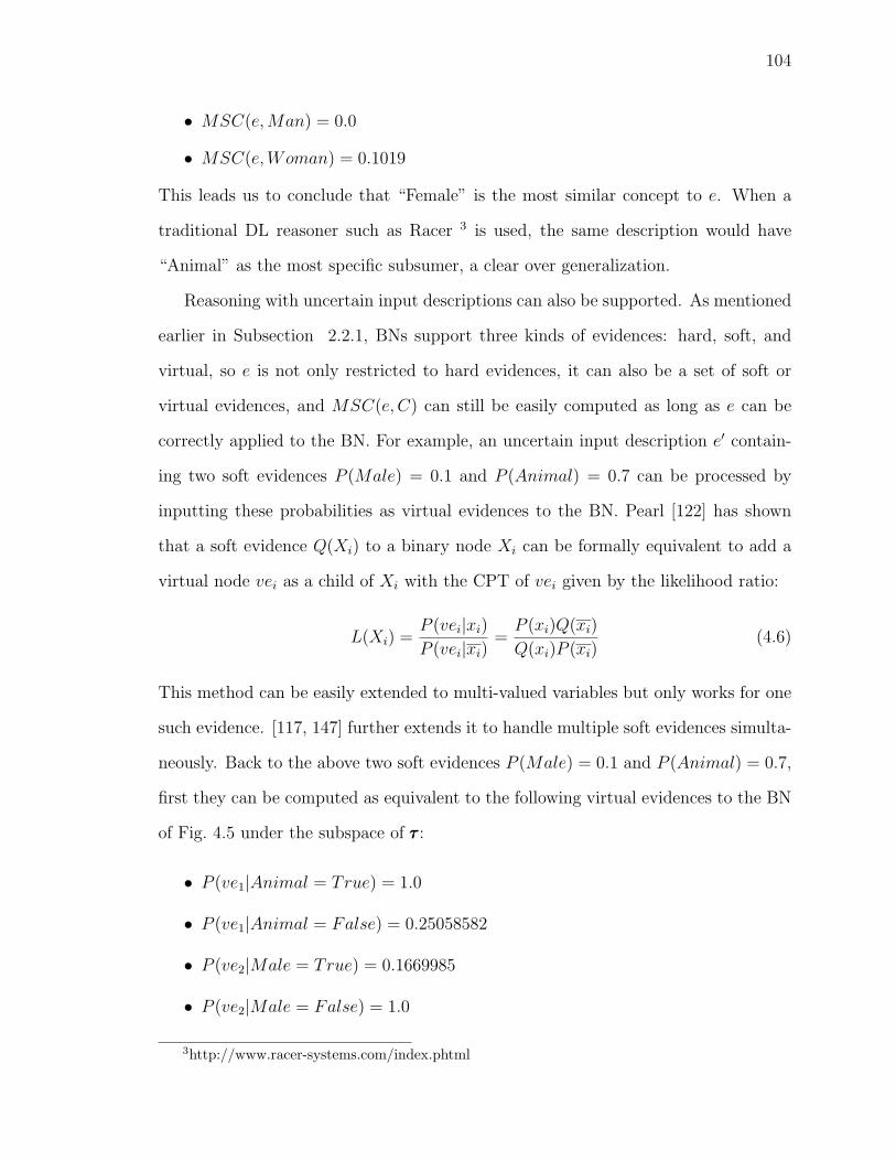
104
• MSC(e,Man) = 0.0
• MSC(e,Woman) = 0.1019
This leads us to conclude that “Female” is the most similar concept to e. When a
traditional DL reasoner such as Racer 3 is used, the same description would have
“Animal” as the most specific subsumer, a clear over generalization.
Reasoning with uncertain input descriptions can also be supported. As mentioned
earlier in Subsection 2.2.1, BNs support three kinds of evidences: hard, soft, and
virtual, so e is not only restricted to hard evidences, it can also be a set of soft or
virtual evidences, and MSC(e, C) can still be easily computed as long as e can be
correctly applied to the BN. For example, an uncertain input description e′ contain-
ing two soft evidences P (Male) = 0.1 and P (Animal) = 0.7 can be processed by
inputting these probabilities as virtual evidences to the BN. Pearl [122] has shown
that a soft evidence Q(Xi) to a binary node Xi can be formally equivalent to add a
virtual node vei as a child of Xi with the CPT of vei given by the likelihood ratio:
L(Xi) =P (vei|xi)
P (vei|xi)=
P (xi)Q(xi)
Q(xi)P (xi)(4.6)
This method can be easily extended to multi-valued variables but only works for one
such evidence. [117, 147] further extends it to handle multiple soft evidences simulta-
neously. Back to the above two soft evidences P (Male) = 0.1 and P (Animal) = 0.7,
first they can be computed as equivalent to the following virtual evidences to the BN
of Fig. 4.5 under the subspace of τττ :
• P (ve1|Animal = True) = 1.0
• P (ve1|Animal = False) = 0.25058582
• P (ve2|Male = True) = 0.1669985
• P (ve2|Male = False) = 1.0
3http://www.racer-systems.com/index.phtml

105
This is illustrated in Fig. 4.7. Similarly, we compute the similarity measure between
e′ and each of the nodes in XC = Animal, Male, Female, Human, Man, Womanusing Eq. 4.5 and get:
• MSC(e′, Animal) = 0.4668
• MSC(e′,Male) = 0.0667
• MSC(e′, Female) = 0.5753
• MSC(e′, Human) = 0.0676
• MSC(e′,Man) = 0.0094
• MSC(e′,Woman) = 0.0611
It can be seen that class “Female” remains the most similar concept to e′, but its
similarity value MSC(e′, Female) now decreases to 0.5753.
CPT
CPT
CPT
CPT
0.0 1.0 False
0.8330015 0.1669985 True
False True
ve2
Male
0.0 1.0 False
0.8330015 0.1669985 True
False True
ve2
Male 0.74941418 0.25058582 False
0.0 1.0 True
False True
ve1
Animal
0.74941418 0.25058582 False
0.0 1.0 True
False True
ve1
Animal
Fig. 4.7: Example I - Uncertain Input to Translated BN
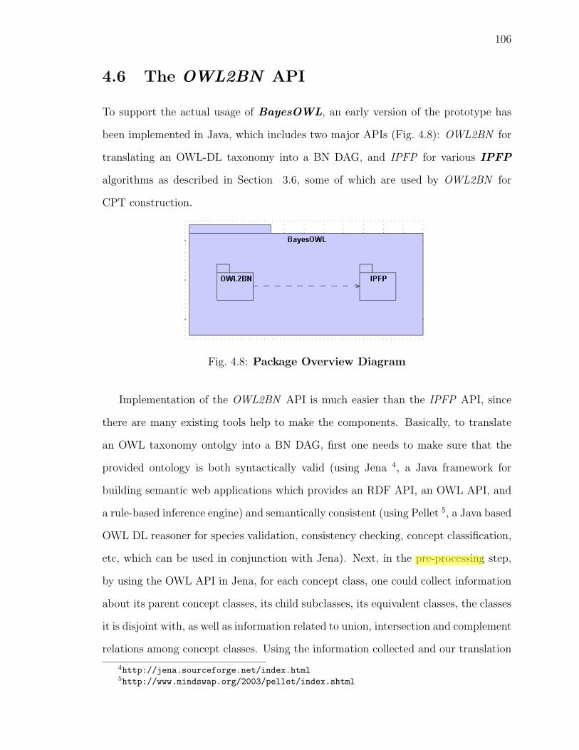
106
4.6 The OWL2BN API
To support the actual usage of BayesOWL, an early version of the prototype has
been implemented in Java, which includes two major APIs (Fig. 4.8): OWL2BN for
translating an OWL-DL taxonomy into a BN DAG, and IPFP for various IPFP
algorithms as described in Section 3.6, some of which are used by OWL2BN for
CPT construction.
Fig. 4.8: Package Overview Diagram
Implementation of the OWL2BN API is much easier than the IPFP API, since
there are many existing tools help to make the components. Basically, to translate
an OWL taxonomy ontolgy into a BN DAG, first one needs to make sure that the
provided ontology is both syntactically valid (using Jena 4, a Java framework for
building semantic web applications which provides an RDF API, an OWL API, and
a rule-based inference engine) and semantically consistent (using Pellet 5, a Java based
OWL DL reasoner for species validation, consistency checking, concept classification,
etc, which can be used in conjunction with Jena). Next, in the pre-processing step,
by using the OWL API in Jena, for each concept class, one could collect information
about its parent concept classes, its child subclasses, its equivalent classes, the classes
it is disjoint with, as well as information related to union, intersection and complement
relations among concept classes. Using the information collected and our translation
4http://jena.sourceforge.net/index.html5http://www.mindswap.org/2003/pellet/index.shtml

107
Fig. 4.9: Architecture of the OWL2BN API

108
rules, one can generate a BN DAG easily using the NeticaJ API, with the CPTs
for L-Nodes assigned as discussed in Section 4.3. With this DAG, and a set of
probabilistic constraints provided, one can use the SD-IPFP algorithm in the IPFP
API to generate CPTs for each concept node. Later, one can use this translated BN
in reasoning, and one could save it into a file. The architecture is shown in Fig. 4.9.
The example shown in Section 4.3 is obtained using this API. The index number
of the L-Nodes starts from zero, and if the ontology provides several disconnected
taxonomies, each will be translated into a BN, though they can be still included in
one .dne file of Netica. Fig. 4.10 and Fig. 4.11 shows the translated BN of a larger
ontology in the nature domain with 71 concept classes defined by “owl:Class” (2 of
them are defined via “owl:intersectionOf”, 1 of them are defined via “owl:unionOf”),
11 “disjoint” relations defined by “owl:disjointWith”, 1 “equivalent” relation defined
by “owl:equivalentClass” and 80 “subclass” relations defined by “rdfs:subClassOf”.
The translated BN, includes 71 concept nodes, 15 L-nodes, and a total number of 84
“superclass → subclass” arcs, the degree of connectivity of each concept node is same
as the “subClassOf” relations 6 that the node is involved with.
The current APIs are provided with Javadocs to be used by developers or re-
searchers who are familiar with Java. The goal of the next version of these APIs is
to design and implement GUI interfaces, which can be used by novice users of Java
or common users who do not know Java at all.
4.7 Comparison to Existing Works
The works closest to BayesOWL [40] are P-CLASSIC [76] and PTDL [159]. One
major difference lies in CPTs. As mentioned earlier in Subsection 2.3.1, neither
P-CLASSIC nor PTDL provides a method to construct CPTs. In contrast, one of
6Here it includes the implicit “subClassOf” relations imposed by “unionOf” and “intersectionOf”relations.

109
Fig. 4.10: An Ontology with 71 Concept Classes, Part 1

110
Fig. 4.11: An Ontology with 71 Concept Classes, Part 2
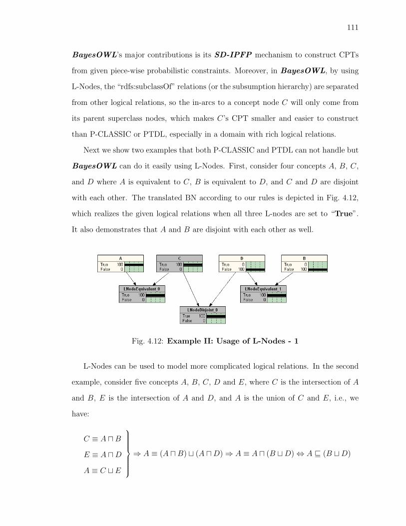
111
BayesOWL’s major contributions is its SD-IPFP mechanism to construct CPTs
from given piece-wise probabilistic constraints. Moreover, in BayesOWL, by using
L-Nodes, the “rdfs:subclassOf” relations (or the subsumption hierarchy) are separated
from other logical relations, so the in-arcs to a concept node C will only come from
its parent superclass nodes, which makes C’s CPT smaller and easier to construct
than P-CLASSIC or PTDL, especially in a domain with rich logical relations.
Next we show two examples that both P-CLASSIC and PTDL can not handle but
BayesOWL can do it easily using L-Nodes. First, consider four concepts A, B, C,
and D where A is equivalent to C, B is equivalent to D, and C and D are disjoint
with each other. The translated BN according to our rules is depicted in Fig. 4.12,
which realizes the given logical relations when all three L-nodes are set to “True”.
It also demonstrates that A and B are disjoint with each other as well.
Fig. 4.12: Example II: Usage of L-Nodes - 1
L-Nodes can be used to model more complicated logical relations. In the second
example, consider five concepts A, B, C, D and E, where C is the intersection of A
and B, E is the intersection of A and D, and A is the union of C and E, i.e., we
have:
C ≡ A uB
E ≡ A uD
A ≡ C t E
⇒ A ≡ (A uB) t (A uD) ⇒ A ≡ A u (B tD) ⇔ A v (B tD)

112
That is, implicitly, A is a subclass of B t D. It is shown that BayesOWL can
handle this correctly, while systems such as P-CLASSIC fail on this. The translated
BN according to our rules is depicted in Fig. 4.13, which fulfills all given logical
relations when all the L-nodes are set to “True”. And we can see that, when both
B and D are “False”, A is also in “False”, that means if an individual o does not
belong to concept B or D, then it must not be an instance of A either, i.e., this is
consistent with A is a subclass of B tD.
Fig. 4.13: Example II: Usage of L-Nodes - 2
Compared to PR-OWL [34] and OWL QM [128], BayesOWL concerns explicitly
more about the set or class memberships and logical relations rather than relationship
among attributes. Also, same as P-CLASSIC and PTDL, BayesOWL uses the
standard BN model, while PR-OWL and OWL QM do not. BayesOWL trades the
expressiveness with the simplicity.
In constrast to BayesOWL, when modeling an RDF(S) concept subsumption,
the arcs in the translated BN by the work of Holi and Hyvonen [67, 68] are pointed
from from child subconcept nodes to parent superconcept nodes. And this work only
deals with the “rdfs:subClassOf” relation.
Also, BayesOWL is not to extend or incorporate into OWL or any other ontology
language or logics with probability theory, but to translate a given ontology to a BN in
a systematic and practical way, and then treats ontological reasoning as probabilistic

113
inferences in the translated BNs. Several benefits can be seen with this approach. It
is non-intrusive in the sense that neither OWL nor ontologies defined in OWL need
to be modified. Also, it is flexible, one can translate either the entire ontology or
part of it into BN depending on the needs. Moreover, it does not require availability
of complete conditional probability distributions, pieces of probabilistic information
can be incorporated into the translated BN in a consistent fashion. With these and
other features, the cost of the approach is low and the burden to the user is minimal.
One thing to emphasis is that BayesOWL can be easily extended to handle other
ontology representation formalisms (syntax is not important, semantic matters), if
not using OWL.
4.8 Summary
This chapter describes the research on developing a probabilistic framework for mod-
eling uncertainty in semantic web taxonomy ontologies based on BNs. We have
proposed a method to encode probabilistic constraints for ontology classes and rela-
tions in OWL. We have also defined a set of rules for translating an OWL taxonomy
ontology into a BN DAG and provided a new algorithm SD-IPFP for efficient con-
struction of CPTs. The translated BN is semantically consistent with the original
ontology and satisfies all given probabilistic constraints. With this translation, on-
tology reasoning can be conducted as probabilistic inferences with potentially better,
more accurate results. Future work includes extending the translation to include
properties, instances and datatypes, and continuing work on ontology mapping based
on BayesOWL which includes addressing the difficult issue of one-to-many mapping
and its generalized form of many-to-many mapping where more than one concepts
need to be mapped from one ontology to another at the same time. The BayesOWL
framework presented in this chapter relies heavily on the availability of probabilis-

114
tic information for both ontology to BN translation and ontology mapping. This
information is often not available (or only partially available) from domain experts.
Learning these probabilities from data then becomes the only option for many ap-
plications. The current focus in this direction is the approach of text classification
[32, 92]. The most important and also most difficult problem in this approach is
to provide high quality sample documents to each ontology class. We are exploring
ontology guided search of the web for such documents. Another interesting direction
for future work is to deal with inconsistent probabilistic information. For example, in
constructing CPTs for the translated BN, the given constraints may be inconsistent
with each other, also, a set of consistent constraints may itself be inconsistent with
the network structure. This issue involves detection of inconsistency, identification of
sources of inconsistency, and resolution of inconsistency.

Chapter 5
Conclusion and Future Work
Dealing with uncertainty is crucial in ontology engineering tasks such as domain mod-
eling, ontology reasoning, and concept mapping between ontologies. In this research
we have developed BayesOWL, a probabilistic extension to OWL that translates
OWL taxonomy ontologies into BNs. We have defined new OWL classes (“Prior-
Prob”, “CondProb”, and “Variable”), which can be used to representing in OWL
the probabilistic constraints concerning the entities and relations in given ontologies.
We have also defined a set of rules for translating OWL ontology taxonomy into
Bayesian network DAG and provided a new algorithm SD-IPFP to construct CPTs
for all concept nodes. SD-IPFP is further developed into E-IPFP and D-IPFP
to modify the CPTs of Bayesian networks from low-dimensional probabilistic con-
straints. We have also implemented an early version of this framework, including an
API for OWL2BN translation and an API for the various IPFP algorithms.
This probabilistic extension to OWL is compatible with OWL-DL semantics, and
the translated BN is associated with a joint probability distribution over the appli-
cation domain that is consistent with given probabilistic constraints.
However, as mentioned earlier in previous chapters, there are a number of issues
remained to be addressed, which lead to several possible future research directions: 1)
extending the translation to include properties and instances; 2) handling inconsistent
probabilistic constraints in the various IPFP algorithms, especially in D-IPFP ; 3)
investigating the scalability issues of BayesOWL in both translation and consequent
reasoning; 4) developing methods to learn probabilities about concepts and their
relations from existing web data; 5) the application of BayesOWL in supporting
ontology mapping. We will briefly discuss each of these issues next.
115

116
1. Dealing with Properties and Instances
An ontology in OWL can define object properties and datatype properties, and
there are also constructs available for properties about properties. Methods from
P-CLASSIC can be directly adopted into our framework, but with a complicated
probability computation mechanism across multiple BNs. However, our goal is to
translate the whole ontology into one single standard Bayesian network so that stan-
dard belief updating algorithm could be used to do the reasoning. The difficulty
comes from the fact that a single concept C may be associated with more than one
probability spaces when C acts in different roles. For example, a concept “Animal”
with an object property “hasParent” (which has “Animal” as its domain and range)
links an individual “a” in “Animal” to another individual “b” in “Animal”, thus,
the probability space of “Animal” as a concept node is different from the probability
space of “Animal” as the range of a concept node. How to connect these two spaces
is the hinge to completely resolve this issue.
BayesOWL is based on the model-theoretic semantics of OWL, so the modeling
of uncertainty is in the granularity of concept classes. Methods from PRM [55] or
DAPER [65] may be borrowed in building a BN based on instances.
2. Dealing with Inconsistent Probabilistic Constraints
The success of the algorithms presented in Chapter 3 relies on the quality of the
probabilistic constraints provided. Among other thing, it is required that the proba-
bilistic constraints must be consistent with each other, and there exists at least one
distribution that can satisfy all the constraints. There are at least three theoretical
issues related to the impact of the input constraint set’s quality on the quality of
solution: 1) Existence: Under what condition will the input constraint set specify a
multivariate joint distribution? 2) Uniqueness: Assume such joint distribution exists,
when will it be unique? 3) Quality of input set: How to deal with weakly consistent,

117
inconsistent or incomplete input constraint set which fails the current algorithms?
3. Investigating Scalability
Scalability is an important issue in both BN translation and consequent reason-
ing, when the application domain becomes large and complex. A real world ontology
may involves hundreds or even thousands of concept definitions and the same scale
of properties and concept relations, the translated BN thus becomes huge and very
complex, and inference in it becomes increasingly more expensive or even practically
intractable using standard exact BN inference algorithms. So the first issue of scala-
bility is with computational complexity when the size of the translated BN becomes
large. To address this issue, one may use some of the existing BN approximate al-
gorithms such as loopy propagation and various stochastic sampling [60]. A more
promising approach, however, would be to reduce the complexity by exploring the
structure of the translated BN. For example, since the BN is translated from ontolo-
gies, interrelations between some or many parts of BN may be sparse, especially if the
given ontology is a taxonomy. Then, as suggested by “Multiply Sectioned Bayesian
Networks” [158] its may be relatively easy to break the BN into small parts or sec-
tions and perform inference distributively in individual modules while maintaining
the coherence over the large BN.
Scalability is less an issue for the translation of a given ontology to BN, the
number of nodes in BN is well controlled (it equals to the number of classes in the
ontology plus the number of logical relations defined over these classes). As discussed
in Chapter 3, SD-IPFP substantially reduces computational complexity for CPT
construction by localizing the computation to one single CPT. However, it may be-
come an issue when the ontology is expanding with additional classes and relations
defined. For structural translation, BayesOWL can easily add new concept nodes
and L-nodes into the DAG of the translated BN without modifying the rest of the

118
existing network structure. However, SD-IPFP, cannot work incrementally to in-
corporate probabilistic constraints concerning newly added classes, we must re-run
the whole process and obtain a new converged distribution based on all constraints
provided (both old and new), so the second issue is to develop an incremental version
of SD-IPFP (and in more general case, D-IPFP and E-IPFP).
Also, compared to E-IPFP, D-IPFP trades I-divergence for efficiency. One
question is, what would be the upper bound of such a sacrifice in I-divergence? In
what range the increase of I-divergence is reasonable or acceptable? This third issue
is related to determining a reasonable Y and S at the technical level. If Y is small,
D-IPFP will in general be faster but the converged distribution is farther away from
the original distribution, compared to that of E-IPFP, the best we can obtained by
both satisfying all probabilistic constraints and the structural constraint.
4. Learning Probabilities from Web Data
The CPT construction of BayesOWL requires prior probability distributions P (C)
to capture the uncertainty about concepts (i.e., how an arbitrary individual belongs
to class C), and conditional probability distributions P (C|D) for relations between
C and D in the same ontology (e.g., how likely an arbitrary individual in class D
is also in D’s subclass C). Further, the framework for ontology mapping (to be
discussed next) requires a set of joint probability distributions P (C,D) for initial
raw semantic similarity between concepts C and D from different ontologies. In
many cases these kinds of probabilistic information are not available and are difficult
to obtain from domain experts. Learning probabilities (i.e., priors about concepts,
conditionals between subconcepts and superconcepts, and raw semantic similarities
between concepts in two different ontologies) from existing web data maybe possible
with the development of search engines such as Google 1, Swoogle 2, Ask Jeeves 3,
1http://www.google.com2http://swoogle.umbc.edu/3http://ask.com/

119
Answers.com 4, etc.
Our initial solution to learning these probabilities is to apply Naive Bayes text
classification technique [32, 92] by explicitly associating a concept with a group of
sample documents (called exemplars) retrieved and selected automatically from World
Wide Web (WWW). The idea is inspired by those machine learning based semantic
integration approaches such as [44, 80, 130] where the meaning of a concept is implic-
itly represented by a set of exemplars that are relevant to it. The rationale is that
the meaning of a concept can be described or defined in the way that it is used.
Learning the probabilities we need from these exemplars is straightforward. First,
we build a model containing statistical information about each concept’s exemplars
in Ontology 1 using a text classifier such as Rainbow 5, and then classify each concept
in Ontology 2 by their respective exemplars using the model of Ontology 1 to obtain
a set of probabilistic scores showing the similarity between concepts. Ontology 1’s
exemplars can be classified in the same way by the model built using Ontology 2’s
exemplars. This cross-classification (Fig. 5.1) process helps find a set of raw mappings
between Ontology 1 and Ontology 2 by setting some threshold values. Similarly, we
can obtain prior or conditional probabilities related to concepts in a single ontology
through self-classification with the model for that ontology.
Fig. 5.1: Cross-Classification using Rainbow
4http://www.answers.com/5http://www-2.cs.cmu.edu/~mccallum/bow/rainbow

120
How to obtain high quality exemplars (both positive and negative) automatically
is a crucial issue. The quality of the learned probabilities is highly dependent on the
quality of the exemplars (e.g., how relevant they are to the concept and how compre-
hensive they are in capturing all important aspects of the concept), and it would be
a very time-consuming task for knowledge workers to choose high quality exemplars
manually. The need to find sufficient relevant exemplars for a large quantity of con-
cepts manually greatly reduces the attractiveness and applicability of these machine
learn-ing based approaches. Our approach is to use search engines such as Google and
Answers.com to retrieve exemplars for each concept node automatically from WWW,
the richest information resource available nowadays. This again introduces several
practical concerns such as how to form the query strings to these engines based on
given ontologies, how to pre-processing the results crawled back from these engines
to include only those most relevant documents?
Even if we obtained highly relevant exemplars successfully, there still remains
one big theoretical issue: the semantics of a concept in a document represents more
close to its meaning in natural language, while in BayesOWL, the semantics of a
concept is based on model-theoretics. For example, if “Woman” and “Man” are two
disjoint concepts, in OWL semantics, they share no instances in common, thus makes
“P (Woman = True|Man = True) = 0”; however, the concept “Woman” and “Man”
in natural language are closely related to each other, using the exemplars associated
with them, the learned probability “P (Woman = True|Man = True)” will never be
zero. Is it possible to find a way to reconcile these two semantics? If it is yes, how?
5. Supporting Ontology Mapping
As surveyed in Section 2.5, semantic heterogeneity between two different applications
or agents comes from their use of conflicted or mismatched terms about concepts. It
has become increasingly clear that being able to map concepts between different,

121
independently developed ontologies is imperative to semantic web applications and
other applications requiring semantic integration. Narrowly speaking, a mapping can
be defined as a correspondence between concept A in Ontology 1 and concept B in
Ontology 2 which share similar or the same semantics. [107] provides a brief survey
on existing approaches for ontology-based semantic integration. Most of these works
are either based on syntactic and semantic heuristics, machine learning (e.g., text
classification techniques in which each concept is associates with a set of text docu-
ments that exemplify the meaning of that concept), or linguistics (spelling, lexicon
relations, lexical ontologies, etc.) and natural language processing techniques.
It is often the case that, when mapping concept A defined in Ontology 1 to Ontol-
ogy 2, there is no concept in Ontology 2 that is semantically identical to A. Instead,
A is similar to several concepts in Ontology 2 with different degree of similarities. A
solution to this so-called one-to-many problem, as suggested by [130] and [43], is to
map A to the target concept B which is most similar to A by some measure. This
simple approach would not work well because 1) the degree of similarity between A
and B is not reflected in Ontology2 and thus will not be considered in reasoning after
the mapping; 2) it cannot handle the situation where A itself is uncertain; and 3)
potential information loss because other similar concepts are ignored in the mapping.
Different from their contributions, we propose a new methodology in supporting
ontology mapping based on BayesOWL. As can be seen from Fig. 5.2, the system
includes four components: 1) a learner to obtain probabilistic ontological information
and initial raw similarities using data obtained from web (as described earlier); 2) a
representation mechanism for the learned uncertain information concerning the enti-
ties and relations in given ontologies (as described in Section 4.1); 3) a BayesOWL
module to translate given taxonomy ontologies (together with the learned uncertain
information) into BNs (as described in Chapter 4); and 4) a concept mapping module
which takes a set of learned initial raw similarities as input and finds new mappings

122
between concepts from two different ontologies as an application of Rong Pan’s for-
malized BN mapping framework [117] for belief propagation between different BNs
that is based on probabilistic evidential reasoning across two BNs.
Fig. 5.2: The Proposed Ontology Mapping Framework
Our preliminary work along this direction and some initial experimental results
can be found at [41, 117]. Here we briefly sketches the BN mapping framework [117]
and its remaining issues to be addressed.
The BN Mapping Framework
What we need in supporting mapping concepts is a framework that allows two BNs
(translated from two ontologies) to exchange beliefs via variables that are similar but
not identical. We illustrate our ideas by first describing how mapping shall be done
for a pair of similar concepts (A from Ontology 1 to B in Ontology 2), and then
discussing issues we face when generalizing such pair-wise mappings to network to
network mapping. We assume the similarity information between A and B is captured

123
by the joint distribution P (A,B). Now we are dealing with three probability spaces:
SA and SB for BN1 and BN2, and SAB for P (A,B). The mapping from A to B
amounts to determining the distribution of B in SB, given the distribution P (A) in
SA under the constraint P (A,B) in SAB.
To propagate probabilistic influence across these spaces, we can apply Jeffrey’s rule
and treat the probability from the source space as soft evidence to the target space
[122, 147]. This rule goes as follow. When the soft evidence on Xi ∈ X, represented
as the distribution Q(Xi), is presented, not only P (Xi), the original distribution of
Xi, is changed to Q(Xi), all other variables Xj 6=i ∈ X will change their distributions
from P (Xj) to Q(Xj) according to Eq. 5.1
Q(Xj) =∑
i
P (Xj|xi)Q(xi) (5.1)
if P (Xj|Xi) is invariant with respect to Q(Xi), where the summation is over all states
xi of Xi.
Fig. 5.3: Mapping Concept A in Ontology1 to B in Ontology2
As depicted in Fig. 5.3, mapping A to B is accomplished by applying Jeffrey’s
rule twice, first from SA to SAB, then SAB to SB. Since A in SA is identical to A in
SAB, P (A) in SA becomes soft evidence Q(A) to SAB and by applying Eq. 5.1 the
distribution of B in SAB is updated to
Q(B) =∑
i
P (B|ai)Q(ai) (5.2)
Q(B) is then applied as soft evidence from SAB to node B in SB, updating beliefs for

124
every other variable V in SB by
Q(V ) =∑j
P (V |bj)Q(bj)
=∑j
P (V |bj)∑i
P (bj|ai)Q(ai)
=∑j
P (V |bj)∑i
P (bj|ai)P (ai)
(5.3)
Back to the example in Fig. 4.5, where the posterior distribution of “Human”,
given hard evidence ¬Male u Animal, is (True 0.102, False 0.898). Suppose we
have another BN which has a variable “Adult” with marginal distribution (True 0.8,
False 0.2). Suppose we also know that “Adult” is similar to “Human” with condi-
tional distribution (“T” for “True”, “F” for “False”)
P (Adult|Human) =
T F
T
F
0.7 0.3
0.0 1.0
Mapping “Human” to “Adult” leads to a change of latter’s distribution from (True 0.8,
False 0.2) to (True 0.0714, False 0.9286) by Eq. 5.2. Such a change can then be
propagated to further update believes of all other variables in the target BN by
Eq. 5.3.
Remaining Issues
Usually, A from Ontology1 maybe semantically similar to more than one concept in
Ontology2. For example, if A is fairly similar to B in Ontology2, it would also be
similar to all super concepts and also some sub-concepts of B, possibly with different
similarity measures. The learned initial raw similarities may include multiple pair-
wise mappings that initiate from A in Ontology1 and end at each similar concept
BJ in Ontology2. Probabilistically, BN2 for Ontology2 can be seen as receiving n
soft evidences, one for a pair-wise mapping from A to BJ for each similar concept
BJ in Ontology2. This requires 1) all similarity measures P (A,BJ) remain invariant,

125
and 2) conditional dependencies among variables in BN2 also remain invariant. How
to extend the previous “1 to 1” mapping to this “1 to n” mapping is the first issue
need to be addressed, that is, we need a mechanism to propagate multiple pair-wise
raw mappings as soft evidences to BN2, and after propagation, all these “1 to 1”
mappings should be held simultaneously across BN1 and BN2.
On the other hand, in theory, any pair of variables between two BNs can be linked,
albeit with different degree of similarities. Therefore we may potentially have n1×n2
raw mappings ( n1 and n2 are the number of variables in BN1 and BN2, respectively).
However, some of these raw mappings maybe be redundant since they can be satisfied
by propagating other raw mappings.
Fig. 5.4: Example of Mapping Reduction
As shown in Fig. 5.4, we have variables A and B in BN1, C and D in BN2, and
raw similarities between every pair as below:
P (C, A) =
0.3 0.0
0.1 0.6
, P (D, A) =
0.33 0.18
0.07 0.42
,
P (D,B) =
0.348 0.162
0.112 0.378
, P (C,B) =
0.3 0.0
0.16 0.54
.
However, we do not need to propagate for all these raw similarities. As Fig. 5.4
depicts, when we have a mapping from A to C, all these raw similarities are satisfied
(the other three mappings are thus redundant). This is because not only beliefs on C,
but also beliefs on D are properly updated by mapping A to C. Several experiments

126
with large BNs have shown that only a very small portions of all n1 × n2 mappings
are needed in satisfying all raw similarities (or, name it “probabilistic constraints”).
This, we suspect, is due to the fact that some of these constraints can be derived from
others based on the probabilistic interdependencies among variables in the two BNs.
So, how to identify and remove redundant mappings by examining the BN structures
and CPTs is the second issue to face.
Given the above issues being successfully addressed, and all initial raw similarities
be properly propagated from BN1 to BN2, we can conduct probabilistic reasoning to
find the best concept matches between Ontology1 and Ontology2. However, some-
times the best match is not between two simple concepts (i.e., between two variables
in BNs), but between a composite concept (i.e, a concept that is defined as a conjunc-
tion (intersection) or disjunction (union) of several variables or their negations) and
a simple concept, or even between two composite concepts. So, the third big issue is
how to calculate joint influence (from multiple variables) from pair-wise mappings to
find this type of complex matches.
6. Other Comments
Besides the above theoretical issues. Another relatively easier but useful work is
to design and develop GUI interfaces for the current prototype implementation and
make it professional enough to be used by other researchers or common users. Also, it
would be very interesting to develop an ontology for standard Bayesian networks, the
development of semantic web lies in the authoring and publishing of as many useful
ontologies as possible on the web.
With the research in these areas to be conducted in the next few years, the work
in this dissertation is potentially useful in practical applications, especially in proba-
bilistic concept subsumption in a single ontology and ontology mapping between two
ontologies.

127
Appendix
A. Ontology for Representing Probabilistic Information
Name: prob.owl
<?xml version=“1.0”?>
<rdf:RDF xmlns:rdf =“http://www.w3.org/1999/02/22-rdf-syntax-ns#”
xmlns:rdfs =“http://www.w3.org/2000/01/rdf-schema#”
xmlns:xsd =“http://www.w3.org/2001/XMLSchema#”
xmlns:owl =“http://www.w3.org/2002/07/owl#”
xmlns:dt =“http://www.cs.umbc.edu/ zding1/owl/dt.xsd#”
xmlns =“http://www.cs.umbc.edu/ zding1/owl/prob.owl#”>
<owl:Ontology rdf:about=“http://www.cs.umbc.edu/ zding1/owl/prob.owl#”>
<owl:versionInfo>v1.0</owl:versionInfo>
</owl:Ontology>
<owl:Class rdf:ID=“Variable”>
<rdfs:subClassOf>
<owl:Restriction>
<owl:onProperty rdf:resource=“#hasClass”/>
<owl:cardinality rdf:datatype=“&xsd;nonNegativeInteger”>1
</owl:cardinality>
</owl:Restriction>
</rdfs:subClassOf>
<rdfs:subClassOf>
<owl:Restriction>
<owl:onProperty rdf:resource=“#hasState”/>
<owl:cardinality rdf:datatype=“&xsd;nonNegativeInteger”>1

128
</owl:cardinality>
</owl:Restriction>
</rdfs:subClassOf>
</owl:Class>
<owl:Class rdf:ID=“States”>
<owl:oneOf rdf:parseType=“Collection”>
<owl:Thing rdf:about=“#True”/>
<owl:Thing rdf:about=“#False”/>
</owl:oneOf>
</owl:Class>
<owl:Class rdf:ID=“ProbObj”/>
<owl:Class rdf:ID=“PriorProb”>
<rdfs:subClassOf rdf:resource=“#ProbObj”/>
<rdfs:subClassOf>
<owl:Restriction>
<owl:onProperty rdf:resource=“#hasVariable”/>
<owl:cardinality rdf:datatype=“&xsd;nonNegativeInteger”>1
</owl:cardinality>
</owl:Restriction>
</rdfs:subClassOf>
<rdfs:subClassOf>
<owl:Restriction>
<owl:onProperty rdf:resource=“#hasProbValue”/>
<owl:cardinality rdf:datatype=“&xsd;nonNegativeInteger”>1
</owl:cardinality>
</owl:Restriction>
</rdfs:subClassOf>

129
</owl:Class>
<owl:Class rdf:ID=“CondProb”>
<rdfs:subClassOf rdf:resource=“#ProbObj”/>
<owl:disjointWith rdf:resource=“#PriorProb”/>
<rdfs:subClassOf>
<owl:Restriction>
<owl:onProperty rdf:resource=“#hasCondition”/>
<owl:minCardinality rdf:datatype=“&xsd;nonNegativeInteger”>1
</owl:minCardinality>
</owl:Restriction>
</rdfs:subClassOf>
<rdfs:subClassOf>
<owl:Restriction>
<owl:onProperty rdf:resource=“#hasVariable”/>
<owl:cardinality rdf:datatype=“&xsd;nonNegativeInteger”>1
</owl:cardinality>
</owl:Restriction>
</rdfs:subClassOf>
<rdfs:subClassOf>
<owl:Restriction>
<owl:onProperty rdf:resource=“#hasProbValue”/>
<owl:cardinality rdf:datatype=“&xsd;nonNegativeInteger”>1
</owl:cardinality>
</owl:Restriction>
</rdfs:subClassOf>
</owl:Class>
<owl:ObjectProperty rdf:ID=“hasCondition”>

130
<rdfs:domain rdf:resource=“#CondProb”/>
<rdfs:range rdf:resource=“#Variable”/>
</owl:ObjectProperty>
<owl:ObjectProperty rdf:ID=“hasVariable”>
<rdfs:domain rdf:resource=“#ProbObj”/>
<rdfs:range rdf:resource=“#Variable”/>
</owl:ObjectProperty>
<owl:ObjectProperty rdf:ID=“hasClass”>
<rdfs:domain rdf:resource=“#Variable”/>
</owl:ObjectProperty>
<owl:ObjectProperty rdf:ID=“hasState”>
<rdfs:domain rdf:resource=“#Variable”/>
<rdfs:range rdf:resource=“#States”/>
</owl:ObjectProperty>
<owl:DatatypeProperty rdf:ID=“hasProbValue”>
<rdf:type rdf:resource=“&owl;FunctionalProperty”/>
<rdfs:domain rdf:resource=“#ProbObj”/>
<rdfs:range rdf:resource=“&dt;between0and1”/>
</owl:DatatypeProperty>
</rdf:RDF>
Name: dt.xsd
<?xml version=“1.0”?>
<xsd:schema xmlns:xsd=“http://www.w3.org/2001/XMLSchema”>
<xsd:simpleType name=“between0and1”>
<xsd:restriction base=“xsd:real”>
<xsd:minInclusive value=“0.0”/>
<xsd:maxInclusive value=“1.0”/>

131
</xsd:restriction>
</xsd:simpleType>
</xsd:schema>
B. An Example Taxonomy Ontology
Name: nature.owl
<?xml version=“1.0”?>
<rdf:RDF xmlns:rdf =“http://www.w3.org/1999/02/22-rdf-syntax-ns#”
xmlns:rdfs =“http://www.w3.org/2000/01/rdf-schema#”
xmlns:xsd =“http://www.w3.org/2001/XMLSchema#”
xmlns:owl =“http://www.w3.org/2002/07/owl#”
xmlns =“http://www.cs.umbc.edu/ zding1/owl/nature.owl#”>
<owl:Ontology rdf:about=“http://www.cs.umbc.edu/ zding1/owl/nature.owl#”>
<owl:versionInfo>v1.0</owl:versionInfo>
</owl:Ontology>
<owl:Class rdf:ID=“Animal”/>
<owl:Class rdf:ID=“Male”>
<rdfs:subClassOf rdf:resource=“#Animal”/>
</owl:Class>
<owl:Class rdf:ID=“Female”>
<rdfs:subClassOf rdf:resource=“#Animal”/>
<owl:disjointWith rdf:resource=“#Male”/>
</owl:Class>
<owl:Class rdf:ID=“Human”>
<rdfs:subClassOf rdf:resource=“#Animal”/>
</owl:Class>
<owl:Class rdf:ID=“Man”>

132
<owl:intersectionOf rdf:parseType=“Collection”>
<owl:Class rdf:about=“#Human”/>
<owl:Class rdf:about=“#Male”/>
</owl:intersectionOf>
</owl:Class>
<owl:Class rdf:ID=“Woman”>
<owl:intersectionOf rdf:parseType=“Collection”>
<owl:Class rdf:about=“#Human”/>
<owl:Class rdf:about=“#Female”/>
</owl:intersectionOf>
</owl:Class>
<owl:Class rdf:about=“#Human”>
<owl:unionOf rdf:parseType=“Collection”>
<owl:Class rdf:about=“#Man”/>
<owl:Class rdf:about=“#Woman”/>
</owl:unionOf>
</owl:Class>
</rdf:RDF>

133
References
[1] A. M. Abdelbar and S. M. Hedetniemi, “Approximating MAPs for belief net-
works in NP-hard and other theorems,” Artificial Intelligence, vol. 102, pp.
21–38, 1998.
[2] S. Agarwal and P. Hitzler, “Modeling fuzzy rules with description logics,” in
Proceedings of Workshop on OWL Experiences and Directions, Galway, Ireland,
November 2005.
[3] Y. Arens, C. A. Knoblock, and W. Shen, “Query reformulation for dynamic
information integration,” Journal of Intelligent Information Systems, vol. 6,
no. 2/3, pp. 99–130, 1996.
[4] N. Ashish and C. A. Knoblock, “Semi-automatic wrapper generation for internet
information sources,” in Conference on Cooperative Information Systems, 1997,
pp. 160–169.
[5] P. Atzeni and R. Torlone, “Schema translation between heterogeneous data
models in a lattice framework,” in Proceedings of the 6th IFIP TC-2 Working
Conference on Database Semantics (DS-6), Atlanta, Georgia, 1995.
[6] P. Avesani, F. Giunchiglia, and M. Yatskevich, “A large scale taxonomy map-
ping evaluation,” in Proceedings of the 4th International Semantic Web Con-
ference (ISWC), Galway, Ireland, November 2005.
[7] F. Baader, D. Calvanese, D. McGuinness, D. Nardi, and P. F. Patel-Schneider,
Eds., The Description Logic Handbook: Theory, Implementation and Applica-
tions. Cambridge University Press, 2003.
134
[8] F. Baader and B. Hollunder, “KRIS: Knowledge representation and inference
system,” SIGART Bulletin, vol. 2, no. 3, pp. 8–14, 1991.
[9] F. Bacchus, Representing and Reasoning with Probabilistic Knowledge. Cam-
bridge, MA: MIT Press, 1990.
[10] S. Bailin and W. Truszkowski, “Ontology negotiation as a basis for opportunis-
tic cooperation between intelligent information agents,” in Proceedings of the
5th International Workshop on Cooperative Information Agents (CIA 2001),
September 2001, pp. 223–228.
[11] ——, “Ontology negotiation between agents supporting intelligent information
management,” in Proceedings of Workshop on Ontologies in Agent-based Sys-
tems (OAS 2001) at ACM Agents 2001 Conference, Montreal, Canada, June
2001.
[12] C. Batini, M. Lenzerini, and S. B. Navathe, “A comparative analysis of method-
ologies for database schema integration,” ACM Computing Surveys, vol. 18,
no. 4, pp. 323–364, December 1986.
[13] R. J. Bayardo, Jr., W. Bohrer, R. Brice, A. Cichocki, J. Fowler, A. Helal,
V. Kashyap, T. Ksiezyk, G. Martin, M. Nodine, M. Rashid, M. Rusinkiewicz,
R. Shea, C. Unnikrishnan, A. Unruh, and D. Woelk, “InfoSleuth: Agent-based
semantic integration of information in open and dynamic environments,” in Pro-
ceedings of the 1997 ACM SIGMOD International Conference on Management
of Data (SIGMOD’97), Tucson, Arizona, 1997, pp. 195–206.
[14] D. Beneventano, S. Bergamaschi, F. Guerra, and M. Vincini, “The MOMIS
approach to information integration,” in Proceedings of the International Con-
ference on Enterprise Information Systems (ICEIS), 2001, pp. 194–198.

135
[15] S. Bergamaschi, S. Castano, S. D. C. D. Vimeracati, and M. Vincini, “An intel-
ligent approach to information integration,” in Proceedings of the International
Conference on Formal Ontology in Information Systems (FOIS-98), Trento,
Italy, 1998, pp. 253–267.
[16] S. Bergamaschi, S. Castano, and M. Vincini, “Semantic integration of semistruc-
tured and structured data sources,” SIGMOD Record, vol. 28, no. 1, pp. 54–59,
1999.
[17] J. Berlin and A. Motro, “Database schema matching using machine learning
with feature selection,” in Proceedings of the Conference on Advanced Informa-
tion Systems Engineering (CAiSE), 2002.
[18] H. H. Bock, “A conditional iterative proportional fitting (CIPF) algorithm with
applications in the statistical analysis of discrete spatial data,” Bull. ISI, Con-
tributed Papers of 47th Session in Paris, vol. 1, pp. 141–142, 1989.
[19] A. Borgida, R. J. Brachman, D. L. McGuinness, and L. A. Resnick, “CLAS-
SIC: A structural data model for objects,” in Proceedings of the 1989 ACM
SIGMOD International Conference on Management of Data, Portland, Ore-
gon, June 1989, pp. 59–67.
[20] R. Brachman and J. Schmolze, “An overview of the KL-ONE knowledge repre-
sentation system,” Cognitive Science, vol. 9, no. 2, 1985.
[21] S. Bressan and C. Goh, “Semantic integration of disparate information
sources over the internet using constraint propagation,” http://context.mit.
edu/∼steph/cp97/cp97.html, 1997.
[22] S. Bressan, C. H. Goh, K. Fynn, M. Jakobisiak, K. Hussein, H. Kon, T. Lee,
S. Madnick, T. Pena, J. Qu, A. Shum, and M. Siegel, “The context interchange
136
mediator prototype,” in Proceedings of the 1997 ACM SIGMOD International
Conference on Management of Data (SIGMOD’97), Tucson, Arizona, United
States, 1997, pp. 525–527.
[23] D. Calvanese, G. D. Giacomo, and M. Lenzerini, “Description logics for infor-
mation integration,” in Computational Logic: Logic Programming and Beyond,
Essays in Honour of Robert A. Kowalski, ser. Lecture Notes in Computer Sci-
ence, A. Kakas and F. Sadri, Eds. Springer Verlag, 2001, pp. 41–60.
[24] D. Calvanese, G. D. Giacomo, M. Lenzerini, D. Nardi, and R. Rosati, “De-
scription logic framework for information integration,” in Proceedings of the
International Conference on Principles of Knowledge Representation and Rea-
soning, Trento, Italy, 1998, pp. 2–13.
[25] ——, “Data integration in data warehousing,” International Journal of Coop-
erative Information Systems, vol. 10, no. 3, pp. 237–271, 2001.
[26] S. Castano and V. de Antonellis, “A schema analysis and reconciliation tool
environment for heterogeneous databases,” in Proceedings of the 1999 Interna-
tional Symposium on Database Engineering & Applications (IDEAS’99). Wash-
ington D.C., USA: IEEE Computer Society, 1999, pp. 53–62.
[27] H. Chalupsky, “Ontomorph: A translation system for symbolic knowledge,”
in Proceedings of the 7th International Conference on Principles of Knowledge
Representation and Reasoning (KR-00), Breckenridge, Colorado, 2000, pp. 471–
482.
[28] M. Ciociou and D. Nau, “Ontology-based semantics,” in Proceedings of the
7th International Conference on Principles of Knowledge Representation and
Reasoning (KR-00), Breckenridge, Colorado, 2000, pp. 539–560.

137
[29] G. F. Cooper, “The computational complexity of probabilistic inference using
bayesian belief network,” Artificial Intelligence, vol. 42, no. 2-3, pp. 393–405,
March 1990.
[30] G. F. Cooper and E. Herskovits, “A bayesian method for the induction of prob-
abilistic networks from data,” Machine Learning, vol. 9, no. 4, pp. 309–347,
1992.
[31] E. Cramer, “Probability measures with given marginals and conditionals: I-
projections and conditional iterative proportional fitting,” Statistics and Deci-
sions, vol. 18, pp. 311–329, 2000.
[32] M. Craven, D. DiPasquo, D. Freitag, A. McCallum, T. Mitchell, K. Nigam,
and S. Slattery, “Learning to construct knowledge bases from the World Wide
Web,” Artificial Intelligence, vol. 118, no. 1-2, pp. 69–114, 2000.
[33] I. Csiszar, “I-divergence geometry of probability distributions and minimization
problems,” The Annuals of Probability, vol. 3, no. 1, pp. 146–158, 1975.
[34] P. C. G. da Costa, K. B. Laskey, and K. J. Laskey, “PR-OWL: A bayesian
ontology language for the semantic web,” in Proceedings of Workshop on Un-
certainty Reasoning for the Semantic Web (URSW) at the 4th International
Semantic Web Conference (ISWC), Galway, Ireland, November 2005, pp. 23–
33.
[35] S. Decker, M. Erdmann, D. Fensel, and R. Studer, “Ontobroker: Ontology based
access to distributed and semi-structured unformation,” in DS-8: Semantic
Issues in Multimedia Systems. Boston, MA: Kluwer Academic Publisher, 1999,
pp. 351–369.
[36] W. E. Deming and F. F. Stephan, “On a least square adjustment of a sam-

138
pled frequency table when the expected marginal totals are known,” Annals of
Mathematical Statistics, vol. 11, pp. 427–444, 1940.
[37] P. Diaconis and S. L. Zabell, “Updating subjective probability,” Journal of the
American Statistical Association, vol. 37, no. 380, pp. 822–830, 1982.
[38] Z. Ding and Y. Peng, “A probabilistic extension to ontology language OWL,”
in Proceedings of the 37th Hawaii International Conference on System Sciences
(HICSS-37), Big Island, HI, January 2004.
[39] Z. Ding, Y. Peng, and R. Pan, “A bayesian approach to uncertainty modeling in
OWL ontology,” in Proceedings of 2004 International Conference on Advances
in Intelligent Systems - Theory and Applications (AISTA2004), Luxembourg-
Kirchberg, Luxembourg, November 2004.
[40] ——, “BayesOWL: Uncertainty modeling in semantic web ontologies,” in Soft
Computing in Ontologies and Semantic Web, ser. Studies in Fuzziness and Soft
Computing, Z. Ma, Ed. Springer-Verlag, 2005.
[41] Z. Ding, Y. Peng, R. Pan, and Y. Yu, “A bayesian methodology towards au-
tomatic ontology mapping,” in Proceedings of the 1st International Workshop
on “Contexts and Ontologies: Theory, Practice and Applications” at AAAI-05,
Pittsburgh, PA, July 2005.
[42] A. H. Doan, P. Domingos, and A. Halevy, “Reconciling schemas of disparate
data sources: A machine-learning approach,” SIGMOD 2001, 2001.
[43] A. H. Doan, J. Madhavan, R. Dhamankar, P. Domingos, and A. Halevy, “Learn-
ing to match ontologies on the semantic web,” The VLDB Journal (Special Issue
on the Semantic Web), vol. 12, no. 4, pp. 303–319, 2003.

139
[44] A. H. Doan, J. Madhavan, P. Domingos, and A. Halevy, “Learning to map
between ontologies on the semantic web,” in Proceedings of WWW 2002, 2002.
[45] ——, “Ontology matching: A machine learning approach,” in Handbook on
Ontologies in Information Systems. Springer-Verlag, 2004, pp. 397–416.
[46] F. M. Donini, M. Lenzerini, D. Nardi, and A. Schaerf, “Reasoning in description
logics,” Principles of Knowledge Representation, pp. 193–238, 1996.
[47] D. Dou, D. McDermott, and P. Qi, “Ontology translation by ontology merging
and automated reasoning,” in Proceedings of EKAW Workshop on Ontologies
for Multi-Agent Systems, 2002.
[48] M. Ehrig and Y. Sure, “Ontology mapping - an integrated approach,” Institute
AIFB, University of Karlsruhe, April 2004.
[49] D. Fensel, I. Horrocks, F. van Harmelen, S. Decker, M. Erdmann, and M. Klein,
“OIL in a nutshell,” in Proceedings of EKAW-2000, 2000.
[50] Y. Fukushige, “Representing probabilistic knowledge in the semantic web,”
Cambridge, MA, USA, 2004, position paper for the W3C Workshop on Se-
mantic Web for Life Sciences.
[51] ——, “Representing probabilistic relations in RDF,” in Proceedings of Work-
shop on Uncertainty Reasoning for the Semantic Web (URSW) at the 4th Inter-
national Semantic Web Conference (ISWC), Galway, Ireland, November 2005.
[52] H. Garcia-Molina, Y. Papakonstantinou, D. Quass, A. Rajararnan, Y. Sagiv,
J. Ullman, V. Vassalos, and J. Widom, “The TSIMMIS approach to mediation:
Data models and languages,” Journal of Intelligent Information Systems, vol. 8,
no. 2, pp. 117–132, 1997.

140
[53] M. Garcıa-Solaco, F. Saltor, and M. Castellanos, “A structure based schema
integration methodology,” in Proceedings of the 11th International Conference
on Data Engineering (ICDE’95), 1995, pp. 505–512.
[54] M. R. Genesereth, A. M. Keller, and O. M. Duschka, “Infomaster: An infor-
mation integration system,” in Proceedings of the 1997 ACM SIGMOD Inter-
national Conference on Management of Data (SIGMOD’97), Tucson, Arizona,
1997, pp. 539–542.
[55] L. C. Getoor, “Learning statistical models from relational data,” Ph.D. disser-
tation, Department of Computer Science, Stanford University, 2002, Advisor:
Daphne Koller.
[56] R. Giugno and T. Lukasiewicz, “P-SHOQ(D): A probabilistic extension of
SHOQ(D) for probabilistic ontologies in the semantic web,” INFSYS, Wien,
Austria, Research Report 1843-02-06, April 2002.
[57] C. H. Goh, S. Bressan, S. Madnick, and M. Siegel, “Context interchange: New
features and formalisms for the intelligent integration of information,” ACM
Transactions on Information Systems, vol. 17, no. 3, pp. 270–270, 1997.
[58] T. R. Gruber, “A translation approach to portable ontology specifications,”
Knowledge Acquisition, vol. 5, no. 2, pp. 199–220, 1993.
[59] N. Guarino, “Semantic matching: Formal ontological distinctions for informa-
tion organization, extraction, and integration,” in SCIE-97: International Sum-
mer School on Information Extraction, London, UK, 1997, pp. 139–170.
[60] H. Guo and W. Hsu, “A survey on algorithms for real-time bayesian network in-
ference,” in Joint AAAI-02/KDD-02/UAI-02 Workshop on Real-Time Decision
Support and Diagnosis Systems, Edmonton, Alberta, Canada, 2002.

141
[61] V. Haarsler, H.-I. Pai, and N. Shiri, “A generic framework for description logics
with uncertainty,” in Proceedings of Workshop on Uncertainty Reasoning for
the Semantic Web (URSW) at the 4th International Semantic Web Conference
(ISWC), Galway, Ireland, November 2005.
[62] F. Hakimpour and A. Geppert, “Resolving semantic heterogeneity in schema
integration: An ontology based approach,” in Proceedings of International Con-
ference on Formal Ontologies in Information Systems (FOIS’01), October 2001.
[63] G. Hall, “Negotiation in database schema integration,” in Americas Conference
on Information Systems, 1995, McGill University.
[64] J. Y. Halpern, “An analysis of first-order logics of probability,” Artificial Intel-
ligence, vol. 46, pp. 311–350, 1990.
[65] D. Heckerman, C. Meek, and D. Koller, “Probabilistic models for relational
data,” Microsoft Corp., Research Report MSR-TR-2004-30, March 2004.
[66] J. Heinsohn, “Probabilistic description logics,” in Proceedings of UAI-94, 1994,
pp. 311–318.
[67] M. Holi and E. Hyvonen, “Probabilistic information retrieval based on concep-
tual overlap in semantic web ontologies,” in Proceedings of Web Intelligence
Symposium at the 11th Finnish AI Conference, September 2004.
[68] M. Holi and Hyvonen, “Modeling degrees of conceptual overlap in semantic
web ontologies,” in Proceedings of Workshop on Uncertainty Reasoning for
the Semantic Web (URSW) at the 4th International Semantic Web Conference
(ISWC), Galway, Ireland, November 2005.
[69] I. Horrocks, “A denotational semantics for standard OIL and instance OIL,”
November 2000.
142
[70] ——, “DAML+OIL: A description logic for the semantic web,” 2002.
[71] I. Horrocks and U. Sattler, “Ontology reasoning in the SHOQ(D) description
logic,” in Proceedings of the 17th International Joint Conference on Artificial
Intelligence (IJCAI), 2001.
[72] E. Hovy, “Combining and standardizing large-scale, practical ontologies for ma-
chine translation and other uses,” in Proceedings of 1st International Conference
on Language Resources and Evaluation, Granada, 1998.
[73] M. Jaeger, “Probabilistic reasoning in terminological logics,” in Proceedings of
KR-94, 1994, pp. 305–316.
[74] Y. Kalfoglou and M. Schorlemmer, “Information flow based ontology mapping,”
in Proceedings of the 1st International Conference on Ontologies, Databases and
Applications of Semantics (ODBASE-02), Irvine, CA, USA, 2002.
[75] A. Kiryakov and K. I. Simov, “Ontologically supported semantic matching,” in
Proceedings of NoDaLiDa-99 Conference, Trondheim, Norway, 1999.
[76] D. Koller, A. Levy, and A. Pfeffer, “P-CLASSIC: A tractable probabilistic de-
scription logic,” in Proceedings of AAAI-97, 1997, pp. 390–397.
[77] D. Koller and A. Pfeffer, “Object-oriented bayesian networks,” in Proceedings
of UAI-97, 1997, pp. 302–313.
[78] ——, “Probabilistic frame-based systems,” in Proceedings of the 15th National
Conference on Artificial Intelligence (AAAI), July 1998.
[79] R. Kruithof, “Telefoonverkeersrekening,” De Ingenieur, vol. 52, pp. E15–E25,
1937.
[80] M. S. Lacher and G. Groh, “Facilitating the exchange of explicit knowledge
through ontology mappings,” in Proceedings of the 4th International Florida
143
Artificial Intelligence Research Society Conference. AAAI Press, 2001, pp.
305–309.
[81] W. Lam and F. Bacchus, “Learning bayesian belief networks: An approach
based on the MDL principle,” Computational Intelligence, vol. 10, no. 3, pp.
269–293, 1994.
[82] K. Laskey, “First-order bayesian logic,” Department of Systems Engineering
and Operations Research, George Mason University,” Technical Report, April
2005.
[83] S. L. Lauritzen and D. J. Spiegelhalter, “Local computation with probabilities
in graphic structures and their applications in expert systems,” Journal of the
Royal Statistical Society: Series B, vol. 50, no. 2, pp. 157–224, 1988.
[84] W. Li and C. Clifton, “Semantic integration in heterogeneous databases using
neural networks,” in Proceedings of the 20th International Conference on VLDB,
Santiago, Chile, 1994, pp. 1–12.
[85] ——, “SemInt: A tool for identifying attribute correspondences in heteroge-
neous databases using neural networks,” Data Knowledge Engineering, vol. 33,
no. 1, pp. 49–84, 2000.
[86] T. Lukasiewicz, “Probabilistic description logic programs,” in Proceedings of
ECSQARU-2005, 2005, pp. 737–749.
[87] ——, “Stratified probabilistic description logic programs,” in Proceedings of
Workshop on Uncertainty Reasoning for the Semantic Web (URSW) at the 4th
International Semantic Web Conference (ISWC), Galway, Ireland, November
2005.

144
[88] R. M. MacGregor and R. Bates, “The LOOM knowledge representation lan-
guage,” USC/Information Science Institute, Technical Report ISI/RS-87-188,
1987.
[89] J. Madhavan, P. A. Bernstein, and E. Rahm, “Generic schema matching with
cupid,” in Proceedings of the 27th International Conference on VLDB, 2001,
pp. 49–58.
[90] T. Mantay and R. Moller, “Content-based information retrieval by computing
least common subsumers in a probabilistic description logic,” in Proceedings of
the ECAI Workshop of Intelligent Information Integration, Brighton, 1998.
[91] M. Mazzieri and A. F. Dragoni, “A fuzzy semantics for semantic web languages,”
in Proceedings of Workshop on Uncertainty Reasoning for the Semantic Web
(URSW) at the 4th International Semantic Web Conference (ISWC), Galway,
Ireland, November 2005.
[92] A. McCallum and K. Nigam, “A comparison of event models for naive bayes
text classification,” in Proceedings of the AAAI-98 Workshop on “Learning for
Text Categorization”, 1998.
[93] D. L. McGuinness, “Explaining reasoning in description logics,” Ph.D. disser-
tation, Rutgers University, New Brunswick, 1996.
[94] D. L. McGuinness, R. Fikes, J. Rice, and S. Wilder, “An environment for
merging and testing large ontologies,” in Proceedings of the 7th International
Conference on Principles of Knowledge Representation and Reasoning (KR-00),
Breckenridge, Colorado, 2000.
[95] S. Melnik, “Declarative mediation in distributed systems,” in Proceedings of In-
ternational Conference on Conceptual Modeling (ER’00), Salt Lake City, Utah,
October 2000.

145
[96] S. Melnik, H. Molina-Garcia, and E. Rahm, “Similarity flooding: A versatile
graph matching algorithm,” in Proceedings of the International Conference on
Data Engineering (ICDE), 2002.
[97] E. Mena, V. Kashyap, A. Illarramendi, and A. Sheth, “Domain specific ontolo-
gies for semantic information brokering on the global information infrastruc-
ture,” in Proceedings of the 1st International Conference on Formal Ontology
in Information Systems (FOIS’98), Trento, Italy, June 1998, pp. 269–283.
[98] T. Milo and S. Zohar, “Using schema matching to simplify heterogeneous data
translation,” in Proceedings of the 24th International Conference on VLDB,
1998, pp. 122–133.
[99] M. Minsky, “A framework for representing knowledge,” June 1974, MIT-AI
Laboratory Memo 306.
[100] ——, “A framework for representing knowledge,” in Readings in Knowledge
Representation, H. J. Levesque, Ed. Los Altos, CA: Morgan Kaufmann, 1987,
pp. 246–262.
[101] P. Mitra, N. F. Noy, and A. R. Jaiswal, “OMEN: A probabilistic ontology map-
ping tool,” in Proceedings of Workshop on Meaning Coordination and Negotia-
tion at the 3rd International Semantic Web Conference (ISWC-04), Hisroshima,
Japan, 2004.
[102] ——, “Ontology mapping discovery with uncertainty,” in Proceedings of the 4th
International Semantic Web Conference (ISWC), Galway, Ireland, November
2005.
[103] P. Mitra, G. Wiederhold, and J. Jannink, “Semi-automatic integration of knowl-
edge sources,” in Proceedings of the 2nd International Conference On Informa-
tion FUSION’99, 1999.

146
[104] P. Mitra, G. Wiederhold, and M. L. Kersten, “A graph-oriented model for
articulation of ontology interdependencies,” in EDBT-00: Proceedings of the
7th International Conference on Extending Database Technology, 2000, pp. 86–
100.
[105] R. Neal, “Connectionist learning of belief networks,” Artificial Intelligence,
vol. 56, pp. 71–113, 1992.
[106] H. Nottelmann and N. Fuhr, “pDAML+OIL: A probabilistic extension to
DAML+OIL based on probabilistic datalog,” in Proceedings of Informa-
tion Processing and Management of Uncertainty in Knowledge-Based Systems
(IPMU), 2004.
[107] N. F. Noy, “Semantic integration: A survey of ontology-based approaches,”
SIGMOD Record, Special Issue on Semantic Integration, vol. 33, no. 4, 2004.
[108] N. F. Noy and M. A. Musen, “PROMPT: Algorithm and tool for automated on-
tology merging and alignment,” in Proceedings of the 17th National Conference
on Artificial Intelligence (AAAI), Austin, TX, 2000.
[109] ——, “Anchor-PROMPT: Using non-local context for semantic matching,” in
Proceedings of Workshop on Ontologies and Information Sharing at IJCAI-
2001, 2001.
[110] ——, “PROMPTDIFF: A fixed-point algorithm for comparing ontology ver-
sions,” in Proceedings of AAAI-2002, Edmonton, Canada, 2002.
[111] J. Ordille, A. Y. Levy, and A. Rajaraman, “Querying heterogeneous information
sources using source descriptions,” in Proceedings of the International Confer-
ence on Very Large Databases, Bombay, India, September 1996, pp. 251–262.

147
[112] L. Palopoli, D. Sacck, G. Terracina, and D. Ursino, “A unified graph-based
framework for deriving nominal interscheme properties, type conflicts and ob-
ject cluster similarities,” in Proceedings of 4th IFCIS International Conference
on Cooperative Information Systems (CoopIS), 1999, pp. 34–45.
[113] L. Palopoli, D. Sacck, and D. Ursino, “An automatic technique for detecting
type conflicts in database schemes,” in Proceedings of the 7th International
Conference on Information and Knowledge Management, Bethesda, Maryland,
United States, November 1998, pp. 306–313.
[114] ——, “Semi-automatic, semantic discovery of properties from database
schemas,” in Proceedings of the 1998 International Symposium on Database
Engineering & Applications (IDEAS’98), 1998, pp. 244–253.
[115] L. Palopoli, G. Terracina, and D. Ursino, “The system DIKE: Towards the semi-
automatic synthesis of cooperative information systems and data warehouses,”
in Proceedings of ADBIS-DASFAA Conference, 2000, pp. 108–117.
[116] J. Z. Pan, G. Stamou, V. Tzouvaras, and I. Horrocks, “f-SWRL: A fuzzy ex-
tension of SWRL,” in Proceedings of the International Conference on Artificial
Neural Networks (ICANN 2005), Special Section on “Intelligent Multimedia and
Semantics”, Warsaw, Poland, 2005.
[117] R. Pan, Z. Ding, Y. Yu, and Y. Peng, “A bayesian network approach to ontology
mapping,” in Proceedings of the 4th International Semantic Web Conference
(ISWC), Galway, Ireland, November 2005.
[118] Y. Papakonstantinou, A. Gupta, and L. Haas, “Capabilities-based query rewrit-
ing in mediator systems,” in Proceedings of the 4th International Conference on
Parallel and Distributed Information Systems, 1996.
148
[119] J. Pearl, “Fusion, propagation, and structuring in belief networks,” Artificial
Intelligence, vol. 29, pp. 241–248, 1986.
[120] ——, “Evidential reasoning using stochastic simulation of causal models,” Ar-
tificial Intelligence, vol. 32, pp. 245–257, 1987.
[121] ——, Probabilistic Reasoning in Intelligent Systems: Networks of Plausible In-
ference. San Mateo, CA: Morgan Kaufman, 1988.
[122] ——, “Jeffery’s rule, passage of experience, and neo-bayesianism,” in Knowledge
Representation and Defeasible Reasoning, H. K. et al., Ed. Kluwer Academic
Publishers, 1990, pp. 245–265.
[123] Y. Peng and Z. Ding, “Modifying bayesian networks by probability constraints,”
in Proceedings of UAI-2005, Edinburgh, Scotland, 2005.
[124] Y. Peng and M. Jin, “A neural netowork approach to approximating MAP in
belief networks,” International Journal of Neural Systems, vol. 12, no. 3-4, pp.
271–290, 2002.
[125] Y. Peng and Z. Zhou, “A neural network learning method for belief networks,”
International Journal of Intelligent Systems, vol. 11, pp. 893–916, 1996.
[126] Y. Peng, Y. Zou, X. Luan, N. Ivezic, M. Gruninger, and A. Jones, “Semantic
resolution for e-commerce,” in Proceedings of the 1st International Joint Con-
ference on Autonomous Agents and Multiagent Systems (AAMAS-02), 2002.
[127] A. Pfeffer, D. Koller, B. Milch, and K. Takusagawa, “SPOOK: A system for
probabilistic object-oriented knowledge representation,” in Proceedings of the
15th Conference on Uncertainty in Artificial Intelligence, 1999.
[128] M. Pool, F. Fung, S. Cannon, and J. Aikin, “Is it worth a hoot? Qualms about
OWL for uncertainty reasoning,” in Proceedings of Workshop on Uncertainty

149
Reasoning for the Semantic Web (URSW) at the 4th International Semantic
Web Conference (ISWC), Galway, Ireland, November 2005.
[129] D. Poole, “Probabilistic horn abduction and bayesian networks,” Artificial In-
telligence, vol. 64, no. 1, pp. 81–129, November 1993.
[130] S. Prasad, Y. Peng, and T. Finin, “A tool for mapping between two ontolo-
gies using explicit information,” in Proceedings of AAMAS-02 Workshop on
Ontologies and Agent Systems, Italy, 2002.
[131] W. V. O. Quine, “On what there is,” Review of Metaphysics, vol. 2, pp. 21–38,
1948.
[132] E. Rahm and P. A. Bernstein, “A survey of approaches to automatic schema
matching,” The VLDB Journal, vol. 10, no. 4, pp. 334–350, 2001.
[133] S. Russell and P. Norvig, Artificial Intelligence, A Modern Approach. Engle-
wood Cliffs, NJ: Prentice Hall, 1995.
[134] A. Sheth and J. Larson, “Federated database systems for managing distributed,
heterogeneous, and autonomous database,” ACM Computing Surveys, vol. 22,
no. 3, pp. 183–236, 1990.
[135] A. P. Sheth, “Changing focus on interoperability in information systems: From
system, syntax, structure to semantics,” in Conference on Interoperating Geo-
graphic Information Systems, 1998.
[136] B. Smith, “Ontology: Philosophical and computational,” http://ontology.
buffalo.edu/smith/articles/ontologies.htm, 2000.
[137] J. F. Sowa, Ed., Principles of Semantic Networks: Explorations in the Rep-
resentation of Knowledge. San Mateo, CA: Morgan Kaufmann Publishers,
1991.

150
[138] G. Stoilos, G. Stamou, V. Tzouvaras, J. Pan, and I. Horrocks, “The fuzzy de-
scription logic f-SHIN,” in Proceedings of Workshop on Uncertainty Reasoning
for the Semantic Web (URSW) at the 4th International Semantic Web Confer-
ence (ISWC), Galway, Ireland, November 2005.
[139] U. Straccia, “Uncertainty and description logic programs: A proposal for ex-
pressing rules and uncertainty on top of ontologies,” CNR Pisa, Technical Re-
port ISTI-2004-TR, 2004.
[140] ——, “A fuzzy description logic for the semantic web,” in Capturing Intelli-
gence: Fuzzy Logic and the Semantic Web, E. Sanchez, Ed. Elsevier, 2005.
[141] H. Stuckenschmidt and U. Visser, “Semantic translation based on approxi-
mate re-classification,” in Proceedings of Workshop on Semantic Approxima-
tion, Granularity and Vagueness, Colorado, USA, 2000.
[142] G. Stumme and A. Maedche, “FCA-Merge: Bottom-up merging of ontologies,”
in Proceedings of 7th International Joint Conference on Artificial Intelligence
(IJCAI), Seattle, WA, 2001, pp. 225–230.
[143] ——, “Ontology merging for federated ontologies on the semantic web,” in
Proceedings of the International Workshop for Foundations of Models for In-
formation Integration (FMII-2001), Viterbo, Italy, 2001.
[144] V. S. Subrahmanian, S. Adah, A. Brink, R. Emery, A. Rajput, R. Ross,
T. Rogers, and C. Ward, “HERMES: A heterogeneous reasoning and mediator
system,” UMCP,” Technical Report, 1996.
[145] A. Tomasic, L. Rashid, and P. Valduriez, “Scaling heterogeneous databases
and the design of DISCO,” in Proceedings of the International Conference on
Distributed Computing Systems, 1995.

151
[146] M. Uschold and M. Gruninger, “Ontologies: principles, methods, and applica-
tions,” Knowledge Engineering Review, vol. 11, no. 2, pp. 93–155, 1996.
[147] M. Valtorta, Y. Kim, and J. Vomlel, “Soft evidential update for probabilistic
multiagent systems,” International Journal of Approximate Reasoning, vol. 29,
no. 1, pp. 71–106, 2002.
[148] W. R. van Hage, S. Katrenko, and G. Schreiber, “A method to combine lin-
guistic ontology-mapping techniques,” in Proceedings of the 4th International
Semantic Web Conference (ISWC), Galway, Ireland, November 2005.
[149] C. J. van Rijsbergen, Information Retrieval, 2nd ed. Lodon:Butterworths,
1979.
[150] R. Vdovjak and G. J. Houben, “RDF based architecture for semantic inte-
gration of heterogeneous information sources,” in Proceedings of International
Workshop on Information Integration on the Web, April 2001.
[151] P. R. S. Visser, D. M. Jones, M. Beer, T. J. M. Bench-Capon, B. Diaz, and
M. J. R. Shave, “Resolving ontological heterogeneity in the KRAFT project,”
in Proceedings of DEXA-99, Florence, Italy, 1999.
[152] J. Vomlel, “Methods of probabilistic knowledge integration,” Ph.D. dissertation,
Department of Cybernetics, Faculty of Electrical Engineering, Czech Technical
University.
[153] ——, “Integrating inconsistent data in a probabilistic model,” Journal of Ap-
plied Non-Classical Logics, pp. 1–20, 2003.
[154] K. von Luck, B. Nebel, C. Peltason, and A. Schmiedel, “The anatomy of the
BACK system,” Techniche Universitat Berlin, KIT-Report 41, January 1987.

152
[155] G. Wiederhold, “Mediators in the architecture of future information systems,”
IEEE Computer, vol. 25, no. 3, pp. 38–49, March 1992.
[156] F. Wiesman, N. Roos, and P. Vogt, “Automatic ontology mapping for agent
communication,” in AAMAS’02: Proceedings of the 1st International Joint
Conference on Autonomous Agents and Multiagent Systems, Bologna, Italy,
2002, pp. 563–564.
[157] D. Woelk, P. Cannata, M. Huhns, N. Jacobs, T. Ksiezyk, R. G. Lavender,
G. Meredith, K. Ong, W. Shen, M. Singh, and C. Tomlinson, “Carnot pro-
totype,” in Object-Oriented Multidatabase Systems: A Solution for Advanced
Applications. Hertfordshire, UK: Prentice Hall International (UK) Ltd., 1995,
pp. 621–651.
[158] Y. Xiang, Probabilistic Reasoning in Multiagent Systems: A Graphical Models
Approach. Cambridge University Press, 2002.
[159] P. M. Yelland, “Market analysis using combination of bayesian networks and
description logics,” Sun Microsystems, Technical Report TR-99-78, 1999.
