-1.0 -0.8 -0.6 -0.4 -0.2 0.0 0.2 0.4 0.6 0.8 1.0

-0.75

-0.50

-0.25

0.00

0.25

0.50

0.75

1.00 Roots of companion matrix

Applied Time Series Econometrics: A Focus on Africa

Alemayehu Geda Njuguna Nudung’u Daniel Zerfu

Addis Ababa University and AERC

© January 2006

1993 1994 1995 1996 1997 1998 1999 2000 20013.6

3.7

3.8

3.9

4.0

4.1

4.2

4.3

ARFIMA (0, d, 8) Model of Kenyan Exchange RateLEX Fitted

-1.0 -0.8 -0.6 -0.4 -0.2 0.0 0.2 0.4 0.6 0.8 1.0

-0.75

-0.50

-0.25

0.00

0.25

0.50

0.75

1.00 Roots of companion matrix

Applied Time Series Econometrics: A Focus on Africa

Alemayehu Geda Njuguna Nudung’u Daniel Zerfu

Addis Ababa University and AERC

© January 2006

1993 1994 1995 1996 1997 1998 1999 2000 20013.6

3.7

3.8

3.9

4.0

4.1

4.2

4.3

ARFIMA (0, d, 8) Model of Kenyan Exchange RateLEX Fitted

Not to be quoted without author’s permission. You may send your comments request for use to AG@ethionet.et

Version 2 December 2005

Applied Time Series Econometrics: A Practical Guide for Macroeconomic

Researchers: A focus on Africa

(With Self-teaching Exposition to Application Software using African Data)

Alemayehu Geda Njuguna Ndung’u

Daniel Zerfu

Department of Economics Addis Ababa University

December, 2005

Table of Contents Chapters Page 1. Introduction

2. Model Specification and Data Exploration 2.1 The Theoretical Model 2.2 Data Exploration 2.3 Narrowing down Research Question and Coping with Model Specification

2.3(a) Narrowing down your research question 2.3(b) Coping with model specifications

2.4 From Model Specification to Estimation

3. Econometric Modelling of Time Series 3.1 Time Series Properties of Macro Variables 3.2 Testing for Unit Root: Practical Hands on 3.3 Cointegration Analysis

3.2.1 Some Relevant Mathematical Notions: Matrices, Eigen values…. 3.2.2 The Engel-Granger (EG) Approach 3.2.3 The Johansen Approach 3.2.4 Identification of the beta-coefficient and Restriction Tests: With one or more cointegrating vector(s)

3.4 VAR and Error Correction Modelling 3.4.1 The Engel-Granger (EG) Approach 3.4.2 The Johansen Approach: With one or more cointegrating vector(s)

4. The Econometric Forecasting:Theory and Application 4.1 Graphic Method of Forecasting 4.2 Modeling Trends, Seasonality and Cycles: MA, AR, ARIMA 4.3 Forecasting with Regression

4.3.1 VAR Model and Forecasting :An Application with Kenyan data 4.3.2 Diagnostic Checks for Forecasting

4.4 Scenarios Analysis and Impulse Response (with EVIWS) 4.5 Application in African Set-up: GDP/Growth Forecasting

5 An Introduction to Panel Cointegration 5.1 Panel Unit Root Tests 5.2 Panel Cointegration Test 5.2.1 Single Equation base Test 5.2.2 Multivariate Equation based Test

5.2.3 Estimation and Inferences in Panel Cointegration Models 5.3 An Application in Africa’s Growth Modelling (Dani) (

6 Modelling an I(2) Variables in African Set-up 6.1 Introduction 6.2 The Production function and Data 6.3 The Econometric Framework 6.4 Empirical Results 6.5 Conclusion

A Guide for Further Readings

Chapter 1: Introduction

Dear Njguna and Daniel, we can draft the introduction along this line. Justification for the work that can be used in drafting the introduction

• The Motivation behind: Inaccessibility of journal articles and some books for Africa applied researchers

• The need to make is self-teaching owing to inability of most government to send their experts at the Ministries of Finance for training

• The need to combine computer software with theoretical teaching • The need to practices using Africa data • The increasing importance of macroeconomic modelling in most African

countries and the role of applied econometrics in that process. • What our target and aim is in working on this book/manual

Under Construction

Chapter 2: Model Specification

2.1 The Theoretical Model

Motivating Your Model

Suppose the researcher wants to examine the determinant (or conditions) of investment in Kenya. When working on this topic you will use your knowledge of econometrics to investigate the macroeconomic determinants of private investment in Kenya. The researcher needs to know the type and frequency of the data and econometrics knowledge, especially of the time series, required in carrying the investigation.

Investment is central to the growth experience of any country. Here you may be required to investigate empirically the determinants of investment. From macroeconomic theory, you know that there are different theories about investment functions. Keynesian theory, for example, explains the dynamics of investment through the accelerator principle, which puts the emphasis on the demand side. In contrast, neoclassical theory emphasizes the supply side by looking at the user cost of capital. Another approach, associated with Tobin, looks at the discrepancy between the market value of productive assets vis-à-vis their replacement costs to explain new investments.

A further perspective on the dynamics of private investment can be obtained by investigating the interaction between public and private investment in an economy. A key question here is whether public investment has a crowding-out or a crowding-in effect on private investment: that is, whether public investment goes at the expense of private investment or, instead, whether it stimulates private investment. One of the currently celebrated empirical regularities is the complementarities between forms of public investment such as infrastructure and private investment. Finally, in a country like Kenya, determining to what extent political factors influence investment behaviour and investment decisions is a further uncertainty that causes complications.

Hence, we can tackle this topic in various ways. In a nut shell, suffice it to say that to write a research paper on this topic you will need to carry out a number of steps:

1) Specify a focused question within this general topic and relate it to relevant theories. 2) Study and summarize the relevant literature on your chosen question. 3) Carry out econometric estimation and hypothesis testing, and evaluate your results in

the light of your research question.

So far, we have emphasized the role of investment in growth and theories of investment as possible motivation for your research. Another source of motivation is an examination of the pattern of the data under analysis. For instance, you may took up a good section of your research paper to analyse the macro variable in question using descriptive analysis and graphs. One aspect to enrich such an analysis is to break down the variable into its various components: in case of investment this could be into fixed investment, inventory, infrastructure (for public investment), and so on. Such detailed descriptive and trend analysis is important to focus on major turning points and the source of such events. Locating Your Study in the Literature and Formulating Testable Empirical Questions To carry out your research you will need to broaden your theoretical reading, say, about investment through a literature survey. Your readings should enable you to formulate your econometric model on the investment function, say, for Kenya or South Africa. This reading needs to be complemented by general reading on the Kenyan and South African economy and on investment behaviour in Kenya and South Africa.

Successful research requires formulating the question you want to investigate in a way that makes investigation possible. At the start of your work, you should spend time thinking about the research question you wish to study and how to make that question manageable. Then, after you have read basic literature and thought through the way authors have set out their research questions, you should try to formulate your questions. You may wish to repeat their research questions and relate them to your data. That is a legitimate scientific procedure. But in most cases, you will need to establish clear value added in the research questions you propose. This is not difficult. It may be that you want to update the data and include a recent period of analysis; it may be that there have been major policy shifts during the update period (such as the 1993 liberalization in Kenya, or the demise of apartheid in South Africa in 1994 or the fall of ‘Socialism’ in 1991 in Ethiopia etc); or it may be that you have discovered weaknesses in other research works. A further constraint on the type of research questions you can deal with in an econometric study relates to the data at your disposal. Clearly, the way you formulate your research question will depend on whether or not the data are available. For example, the database may not allow you to estimate sectoral investment functions (that is, separate functions for agriculture, mining, manufacturing, and so on), but you may distinguish between private and public investment. Similarly, you may find it difficult to estimate Tobin’s (1969) q-model for Kenya because data on replacement costs are not usually available but can be done for South Africa. Hence, when thinking about a research question, take account of the data at your disposal and decide how to make the best use of them. 2.2 Data Exploration with STATA: A Brief View As noted by Wuyts (1992) many published articles covey the message that the researcher began with clear cut hypothesis, tested it, and obtained the reported result. Any ad hock

tampering with the hypothesis is taken as data mining and carefully left out. Such research method is rooted in the methodology which is referred as Popperian (following the works of Karl Popper). However, the real process is a bit messy and involves a lot more trial and error. The latter is hardly reported, however. In fact, as Wuyts noted, when researchers and students fail to find a confirmation to their initial hypothesis they began to get frustrated. Even getting a confirmation to the initial hypothesis doesn’t confirm the possibility of having an alternative explanation which fits the data just as well (Wuyts 1992). Such problems could be, however, avoided by resorting to another approach to data analysis which is rooted in the method of ‘inference to the best explanation’ whose essential ingredient is proper data exploration. ‘Inference to the best explanation’ departs from the Popperian one in favour of a realist approach. It is our view that the adoption of such an approach represents a much more fruitful avenue of research in developing countries. This methodological framework is informed by the works of Harman (1965), Lipton (1991), Mukhrjee and Wuyts (1991), Wuyts (1992a, 1992b) and Lawson (1989). The overall framework is Harman’s (1965) ‘inference to the best explanation’ (contrastive inference), which looks for residual differences in similar histories of facts and foils as a fruitful method for determining a likely cause (Lipton, 1991:78; Mukhrjee and Wuyts 1991). This approach entails testing competing hypotheses in the process of research. At a practical level, this general approach could be narrowed down to a more refined one proposed by Mukhrjee and Wuyts (1991) in which a working hypothesis, is confronted with the evidence and various rival explanations. Wuyts (1992b) argues ‘the best way to test an idea (wrapped up as a hypothesis) is not merely to confront it with its own evidence, but to compare it with rival explanations. It then becomes easier to detect which explanation has more loose ends or will need to resort to ad hoc justifications to cope with criticism’ (Wuyts, 1992b: 4). Once a working hypothesis has been arrived at, the dialogue between data and alternative explanations may best be handled by exploratory data analysis, which comprises graphical display, techniques of diagnostic analysis and transformation of data (Mukherjee and Wuyts, 1991: 1). This does not imply that theory has no role to play. Rather, that theory is important ‘as a guide to pose interesting questions which we shall explore with data’ (Wuyts, 1992a: 2). The generation of working hypotheses, and the subsequent examination of these, may be pursued along Kaldorian lines (Lawson 1989, Lawson et al 1996). In this realist approach to economic analysis, the researcher is free to start from ‘stylized’ facts - broader tendencies ignoring individual details – and to construct a working hypothesis, which fits with these facts. The final stage of the analysis entails subjecting the entities postulated at the modelling or explanatory stage to further scrutiny (Lawson 1989). Data exploration is a pre-requisite for good model formulation. This is because one has to know the pattern of the data in order to give it a mathematical form (ie., to model it). Data exploration and inference, as we noted above, comprises three major techniques:

a) Graphical inspection, b) Data transformation, and c) Diagnostic Analysis

a) Graphical Inspection and Transformation

Data exploration needs to be guided by two guiding principles (Wuyts 1992):

(i) Use numerical summaries along with graphical displays: they complement each other and allow the data to talk back to you;

(ii) Pay attention to outliers and influential points. They are not necessarily a nuisance but can be a source of valuable hints and cues.

Graphical analysis can be done using scattered plots, plots of variable on time and similar data inspection techniques. Transformation of the variable, in particular to a logarithmic form, not only helps to show influential points in a very sharp manner, but also corrects skewed to the right distribution towards normality – a correction relevant in the context of regression analysis. A very versatile graph in STAT is the scatter plot. You may have the scatter plot using the simple STATA command ‘graph’ followed by the name of the variables to be plotted, such as X and Y. Thus, go to your STATA file and type the command: graph X, Y. This will offer you the following graph (see Figure 2.2(a)). STATA has also a facility to weight (analytical weight: aweight; frequency weight: fweight; sampling weights: pweight and importing weight: iweight) your data and label the plot. For instance if you like to have the importance weight by density and also want to label the Y axis by 0, 10, 20, 30, 40 and 50; while the X axis by 0, 10, 20, and 30; and have the title ‘Weighted Scatter Plot’, you may use the following command:

graph X Y[iweight=density], ylable (0,10,20,30,40,50) xlable(0,10,20,30) tiltle(Weighted Scatter Plot).

Figure 2.2(a): Scatter Plot of Ethiopian Debt (1970-2001)

020

0040

0060

0080

0010

000

Eth

iopi

a

1970 1980 1990 2000countryname

Another interesting scatter plot which is excellent for data exploration is the scatter plot matrix (see Figure 2.2(b)) which can be generated using the command

Graph X Y Z G F, matrix labor symbol(p) . The result is given in Figure 2.2(b) Figure 2.2(b): Scatter plot Matrix of Debt for Some Africa Countries (1970-2001)

Burundi

Chad

Ghana

Kenya

0

500

1000

0 500 1000

0

500

1000

0 500 1000

0

2000

4000

6000

0 2000 4000 60000

2000

4000

6000

0 2000 4000 6000

Another extremely important scatter plot is what is called ‘a two way sctterplot’ which can have boxplots in the margin. Such scatterplots are important to make an inference about the nature of the distribution of the variable in question. This latter information is important to help decide on whether the variable needs transformation to come to normality or not. You may use the following command to generate such scatter plots and boxplots:

graph X Y, twoway oneway box title(Scatterplot with Marginal Boxplot and Oneway Scatterplot).

You may also generate boxplots directly by using the command: graph X, box Such box plots (see Figure 2.2(c)) are helpful to understand the distribution characteristic of a series such as debt by African countries offered as Figure 2.2(b). Note for instance that the Ethiopian and Kenyan debt is relatively normally distributed while the other variables show some degree of skewness. When you run a regression and you want to check whether the error term (which is a linear combination of the dependent and explanatory variables) is normally distributed – which is the requirement in classical regression - you could learn a great deal from the box plot which of the variables could be possible sources of non-normality.

Figure 2.2(c): Boxplots of Debt for some African Countries (1970-2001)

02,

000

4,00

06,

000

8,00

010

,000

Ghana EthiopiaKenya Chad

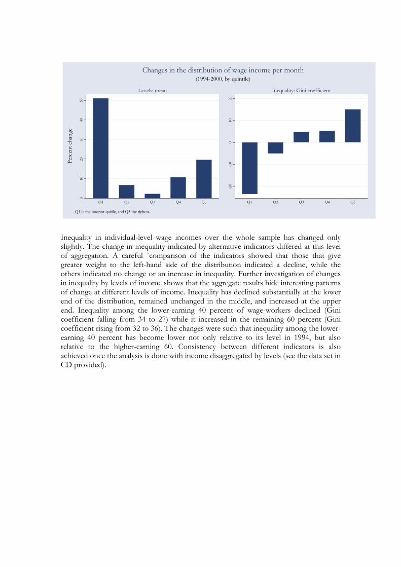
Use of summary statistics (such as mean and median, quintiles etc) creatively is another dimension of data exploration. We illustrate this form Alemayehu and Alem’s (2006) study of labour market in Ethiopian using household level data. As can be read from the summary statistic given on Table 6, Median wage income was unchanged between the two rounds (1994 and 2000) at about 250.00 Birr, while mean incomes changed from about Birr 331.00 to Birr 386. The stagnation in median incomes, however, hides the changes that occurred at the lower and higher ends of the wage distribution. A more disaggregated comparison of changes in income across the rounds indicates that the largest percentage change in wage income occurred in the first (lowest) and fifth (richest) quintiles, and the smallest change in the third quintile. This pattern of change has important implications for the evolution of indicators of poverty. Given the observed level of head-count ratios, larger changes in poverty indicators would have occurred if changes in incomes were concentrated around the middle of the distribution instead of the extremes. In simple words the growth occurred doesn’t seem to be pro-poor or distributional neutral as can be read from Table 6 below. Table 1: Level and inequality of wage incomes: changes between 1994 and 2000

Gini Mean Median 1994 2000 Change % 1994 2000 Change % 1994 2000 Change % Q1 30.96 23.71 -7.25 -23.41 42.45 64.11 21.66 51.02 38.44 65.99 27.55 71.66 Q2 10.69 10.15 -0.54 -5.04 136.99 146.20 9.21 6.72 134.56 142.99 8.43 6.27 Q3 8.95 9.38 0.43 4.81 249.42 254.84 5.41 2.17 250.00 246.50 -3.50 -1.40 Q4 8.31 8.75 0.44 5.28 405.55 448.94 43.39 10.70 400.00 441.70 41.70 10.43 Q5 23.56 27.10 3.54 15.02 857.08 1025.08 168.00 19.60 689.70 759.49 69.79 10.12

010

2030

4050

Q1 Q2 Q3 Q4 Q5

Levels: mean

-20

-10

010

20

Q1 Q2 Q3 Q4 Q5

Inequality: Gini coefficient

Perc

ent c

hang

e

Q1 is the poorest quitile, and Q5 the richest.

(1994-2000, by quintile)Changes in the distribution of wage income per month

Inequality in individual-level wage incomes over the whole sample has changed only slightly. The change in inequality indicated by alternative indicators differed at this level of aggregation. A careful `comparison of the indicators showed that those that give greater weight to the left-hand side of the distribution indicated a decline, while the others indicated no change or an increase in inequality. Further investigation of changes in inequality by levels of income shows that the aggregate results hide interesting patterns of change at different levels of income. Inequality has declined substantially at the lower end of the distribution, remained unchanged in the middle, and increased at the upper end. Inequality among the lower-earning 40 percent of wage-workers declined (Gini coefficient falling from 34 to 27) while it increased in the remaining 60 percent (Gini coefficient rising from 32 to 36). The changes were such that inequality among the lower-earning 40 percent has become lower not only relative to its level in 1994, but also relative to the higher-earning 60. Consistency between different indicators is also achieved once the analysis is done with income disaggregated by levels (see the data set in CD provided).

A

B

C D

0.1

.2.3

.4

2 4 6 8 10log(Wage income)

1994 2000

Individual-level

0.1

.2.3

.4

2 4 6 8 10log(HH wage income)

1994 2000

Household-level

(1994 and 2000)Kernel density estimates: Wage income

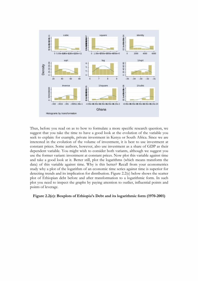
Once you have explored your data using data exploration techniques outlined in your STATA manual, you need to move towards modelling the pattern of data that you have observed thus far. Transformation is also crucial when we plan to model (or give a mathematical form) the pattern of data that we managed to read from carrying out data exploration using various techniques such as scatter plots. STATA’s function ‘gladder’ followed by the name of the variable of interest offers an array of functional forms and their possible distribution in the process of searching for a function form for your model (see Figrue 2.2(d)). From figure 2.2(d) we note that the logarithmic transformation of the variable seems to offer the best approximation for normal distribution.

Figure 2.2(d): Functional Forms that may Fit Ghana’s Pattern of Debt (1970-2001)

05.0e

-12

1.0e

-11

1.5e

-11

2.0e

-11

0 5.00e+101.00e+111.50e+112.00e+11

cubic

02.0e

-08

4.0e

-08

6.0e

-08

8.0e

-08

1.0e

-07

0 1.00e+072.00e+073.00e+074.00e+07

square

02.0

e-044.

0e-0

46.

0e-0

4

0 2000 4000 6000

identity

0.0

1.02

.03.

04

20 40 60 80

sqrt

0.2

.4.6

6 7 8 9

log

020

4060

80

-.05 -.04 -.03 -.02 -.01

1/sqrt

050

0100

0150

0

-.002 -.0015 -.001 -.0005-1.08e-19

inverse02.

0e+0

54.

0e+0

56.

0e+0

58.

0e+0

5

-4.00e-06-3.00e-06-2.00e-06-1.00e-06-4.24e-22

1/square

02.0

e+084.0e

+08

6.0e

+08

-8.00e-09-6.00e-09-4.00e-09-2.00e-09-1.24e-24

1/cubic

Den

sity

GhanaHistograms by transformation

Thus, before you read on as to how to formulate a more specific research question, we suggest that you take the time to have a good look at the evolution of the variable you seek to explain: for example, private investment in Kenya or South Africa. Since we are interested in the evolution of the volume of investment, it is best to use investment at constant prices. Some authors, however, also use investment as a share of GDP as their dependent variable. You might wish to consider both variants, although we suggest you use the former variant: investment at constant prices. Now plot this variable against time and take a good look at it. Better still, plot the logarithms (which means transform the data) of this variable against time. Why is this better? Recall from your econometrics study why a plot of the logarithm of an economic time series against time is superior for detecting trends and its implication for distribution. Figure 2.2(e) below shows the scatter plot of Ethiopian debt before and after transformation to a logarithmic form. In such plot you need to inspect the graphs by paying attention to outlier, influential points and points of leverage.

Figure 2.2(e): Boxplots of Ethiopia’s Debt and its logarithmic form (1970-2001)

56

78

9lo

geht

i

020

0040

0060

0080

0010

000

Eth

iopi

a

1970 1980 1990 2000countryname...

Ethiopia logehti

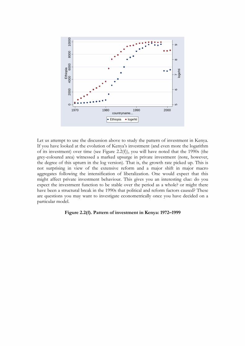
Let us attempt to use the discussion above to study the pattern of investment in Kenya. If you have looked at the evolution of Kenya’s investment (and even more the logarithm of its investment) over time (see Figure 2.2(f)), you will have noted that the 1990s (the grey-coloured area) witnessed a marked upsurge in private investment (note, however, the degree of this upturn in the log version). That is, the growth rate picked up. This is not surprising in view of the extensive reform and a major shift in major macro aggregates following the intensification of liberalization. One would expect that this might affect private investment behaviour. This gives you an interesting clue: do you expect the investment function to be stable over the period as a whole? or might there have been a structural break in the 1990s that political and reform factors caused? These are questions you may want to investigate econometrically once you have decided on a particular model.

Figure 2.2(f). Pattern of investment in Kenya: 1972–1999

0

20

40

60

80

100

120

72 74 76 78 80 82 84 86 88 90 92 94 96 98

0

1

2

3

4

5

72 74 76 78 80 82 84 86 88 90 92 94 96 98

Investment (bln Ksh)

ln (Investment)

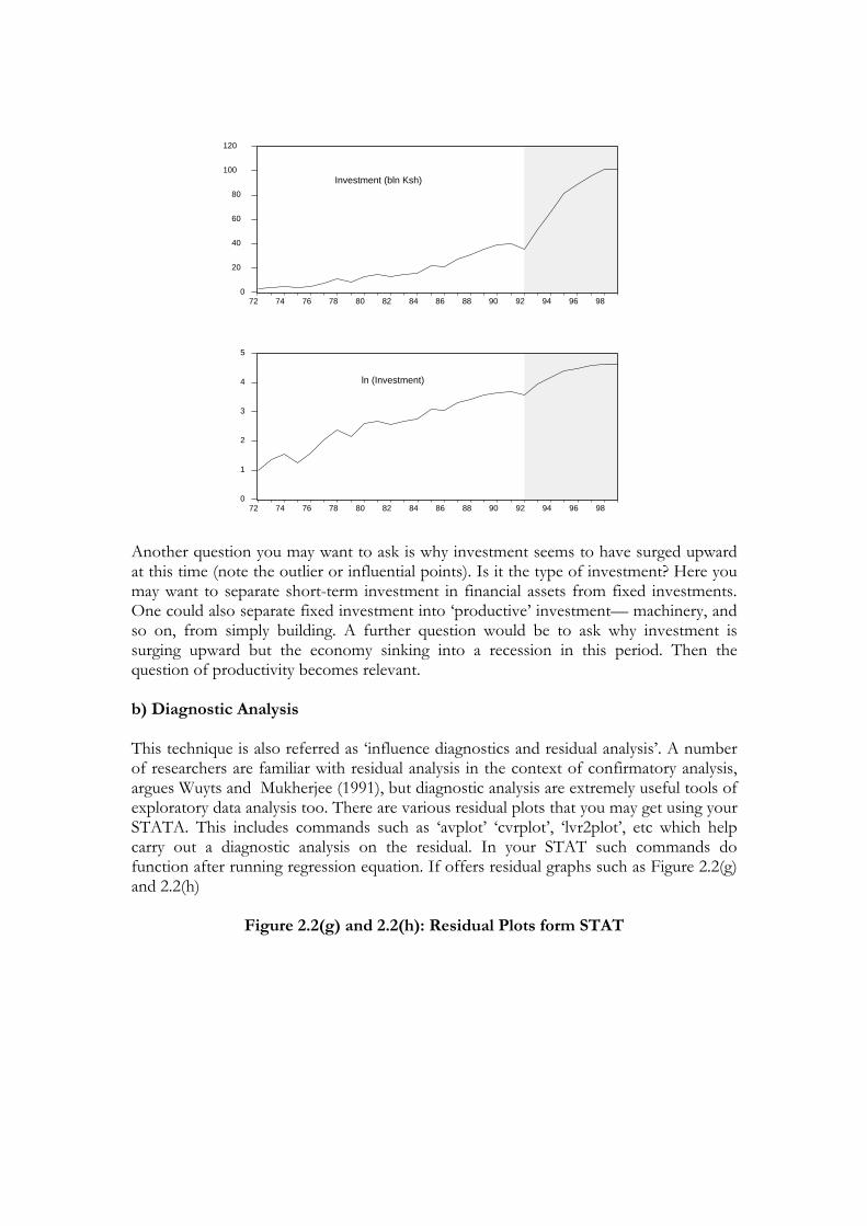
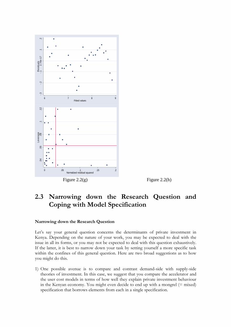
Another question you may want to ask is why investment seems to have surged upward at this time (note the outlier or influential points). Is it the type of investment? Here you may want to separate short-term investment in financial assets from fixed investments. One could also separate fixed investment into ‘productive’ investment— machinery, and so on, from simply building. A further question would be to ask why investment is surging upward but the economy sinking into a recession in this period. Then the question of productivity becomes relevant. b) Diagnostic Analysis This technique is also referred as ‘influence diagnostics and residual analysis’. A number of researchers are familiar with residual analysis in the context of confirmatory analysis, argues Wuyts and Mukherjee (1991), but diagnostic analysis are extremely useful tools of exploratory data analysis too. There are various residual plots that you may get using your STATA. This includes commands such as ‘avplot’ ‘cvrplot’, ‘lvr2plot’, etc which help carry out a diagnostic analysis on the residual. In your STAT such commands do function after running regression equation. If offers residual graphs such as Figure 2.2(g) and 2.2(h)

Figure 2.2(g) and 2.2(h): Residual Plots form STAT

-.3-.2

-.12.

78e-

17.1

.2R

esid

uals

6 7 8 9Fitted values

.04

.06

.08

.1.1

2Le

vera

ge

0 .05 .1 .15 .2Normalized residual squared

Figure 2.2(g) Figure 2.2(h)

2.3 Narrowing down the Research Question and Coping with Model Specification

Narrowing down the Research Question Let’s say your general question concerns the determinants of private investment in Kenya. Depending on the nature of your work, you may be expected to deal with the issue in all its forms, or you may not be expected to deal with this question exhaustively. If the latter, it is best to narrow down your task by setting yourself a more specific task within the confines of this general question. Here are two broad suggestions as to how you might do this. 1) One possible avenue is to compare and contrast demand-side with supply-side

theories of investment. In this case, we suggest that you compare the accelerator and the user cost models in terms of how well they explain private investment behaviour in the Kenyan economy. You might even decide to end up with a mongrel (= mixed) specification that borrows elements from each in a single specification.

2) Another avenue is to examine whether public investment crowds out or crowds in private investment. That is, your specific research question will be to assess the impact of public investment on private investment.

Each of these avenues gives your research a more limited task. The former involves comparing how well different theories of investment explain the empirical evidence; the latter investigates a specific policy question. In each case, however, it is important to think carefully about the specification of your model. Which variables should you include? Should you use log-transformed variables or not? How should you deal with lagged variables? What are the expected signs of the coefficients in the model? Which hypotheses are interesting to test? Is the model stable across the period as a whole? As to the last question, we suggest that you investigate specifically whether model stability pertained during the 1990s. To do this, you can use Chow’s test or some other technique. Alternatively, you may wish to use dummy variables to single out the 1990s. The important point is not just to introduce dummies but also to explain their meaning. Before you introduce dummies, it is always advisable to estimate the model recursively, understand the profile of the coefficients estimated, and then locate the effect the dummies will have in stabilizing the coefficients. Coping with model specifications Specifying a model is a task that requires skill and experience. This is particularly true when we work with time-series data, where we often use lagged variables to denote that what happened in the past has repercussions for the present. For example, in dealing with investment functions, you may wish to try out a specific type of models that aims to capture the fact that adjustment is neither smooth nor immediate. This is the partial adjustment model. On the other hand, to be able to deal with the problem of crowding in or out of private investment by public investment, it is necessary to bring public investment explicitly into the picture as an explanatory variable. You may do this in the context of a mixed specification using a partial adjustment model. You may wish to try out your own pet theory instead. When dealing with the crowding-in–crowding-out hypothesis, it matters what assumptions you make about the lags of the explanatory variables. The important point is that your assumptions about these lags should be reasonable. For example, on the one hand, private investors may immediately react to initiating construction of new infrastructure that may take time to complete, or they may respond with a certain lag after its completion. On the other hand, high levels of government investment may reduce private capital’s access to finance. For these reasons, it is advisable to try out various lags (say, zero to five years) to check the effect of public investment on private investment. In Kenya, for instance, we found current and five-year lagged public investment have statistically significant (positive) impact on private investment. 2.4 From model specification to estimation It is one thing to have specified your theoretical model but quite another to estimate it. Estimation requires not only skill but also patience. Since most macro models rely on time-series data, we will focus on estimation based on time series data, that is, on

macroeconometrics. We will use data from Kenya, Mozambique and Ethiopia to motivate the exposition. The first main point to note at estimation stage is that econometrics is not a mechanical procedure. You need to withdraw yourself from the mechanics of it and see the whole issue from a wider perspective, and in particular, in light of the questions posed at the beginning of your inquiry. The second important point is that since you are confronting your theory with data at this stage, you have a lot of room to modify it in the light of those data—you should repeatedly move back and forth between data and theory. This means going back to your original theory to revise it further, coming back to your data with the revised theory . . . and so on. In this interactive process, you need to make sure that each of your move back and forth is a justifiable move. You should not simply move mechanically from unit root test, to cointegration, to error-correction modelling, to theory and so on. Each step should justify your conclusions at every stage. The details of this estimation technique and its application are taken up in the next chapter.

Chapter 3: Econometric Modelling of Time Series

3.1 Time Series Properties of Macro Variables