applied numerical methods partial diﬀerential...

Applied Numerical Methods

Partial Differential Equations

Abu Hasan Abdullah

October 22, 2008

Abu Hasan Abdullah « 2008

Equation for Conic Section

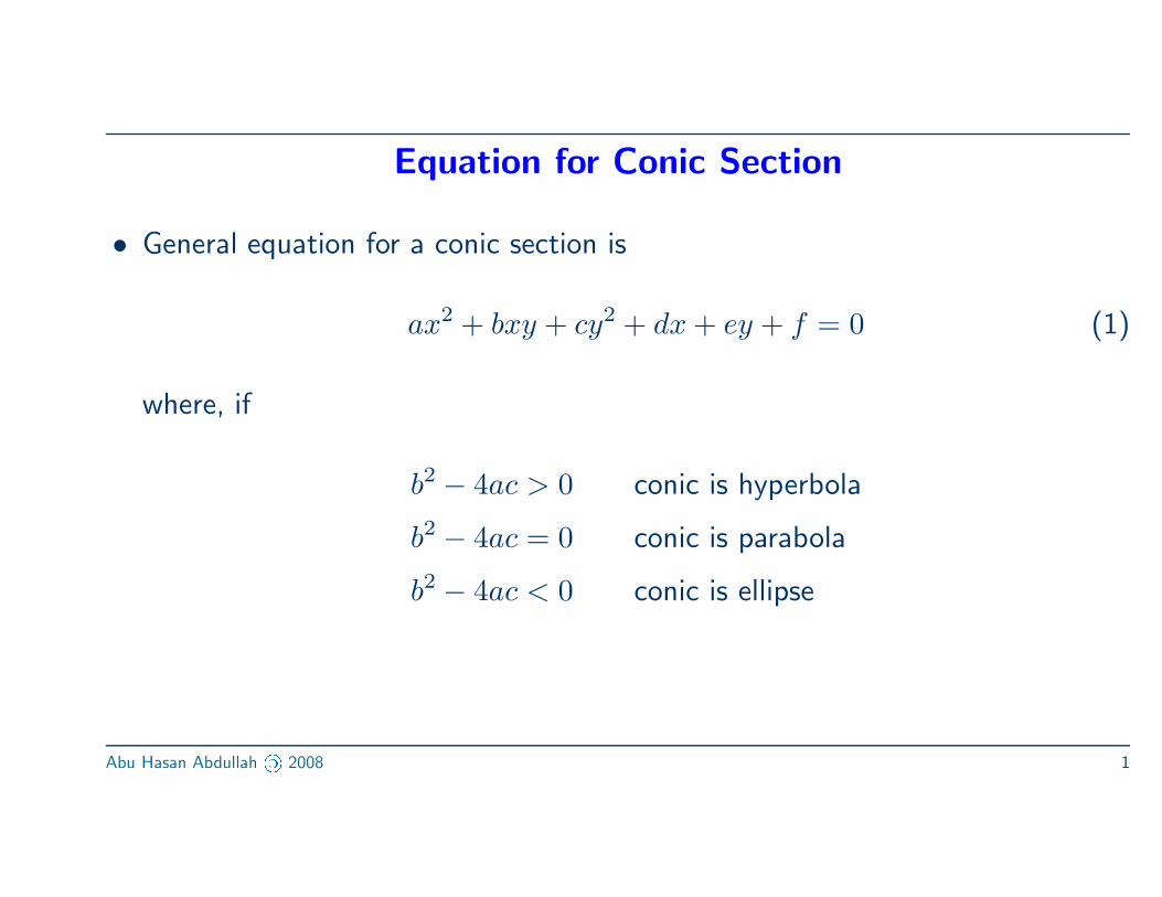
• General equation for a conic section is

ax2 + bxy + cy2 + dx + ey + f = 0 (1)

where, if

b2− 4ac > 0 conic is hyperbola

b2− 4ac = 0 conic is parabola

b2− 4ac < 0 conic is ellipse

Abu Hasan Abdullah « 2008 1

Classification of PDE

Conic Section Analog

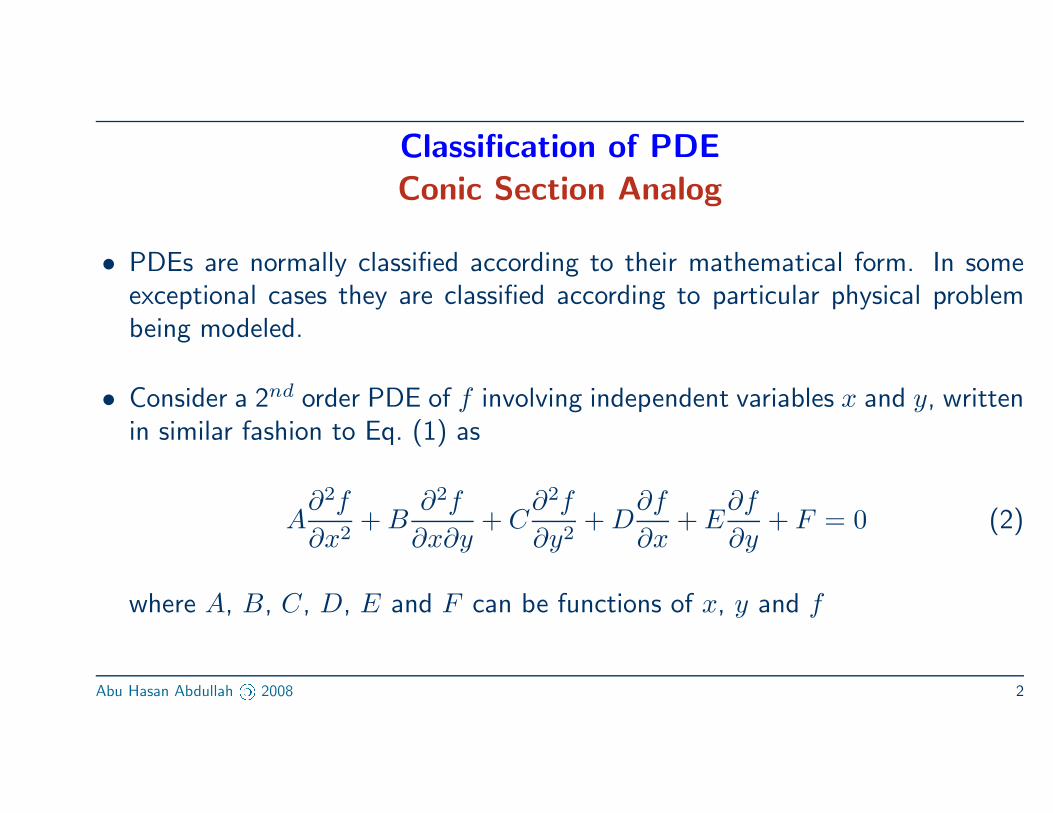
• PDEs are normally classified according to their mathematical form. In someexceptional cases they are classified according to particular physical problembeing modeled.

• Consider a 2nd order PDE of f involving independent variables x and y, writtenin similar fashion to Eq. (1) as

A∂2f

∂x2+ B

∂2f

∂x∂y+ C

∂2f

∂y2+ D

∂f

∂x+ E

∂f

∂y+ F = 0 (2)

where A, B, C, D, E and F can be functions of x, y and f




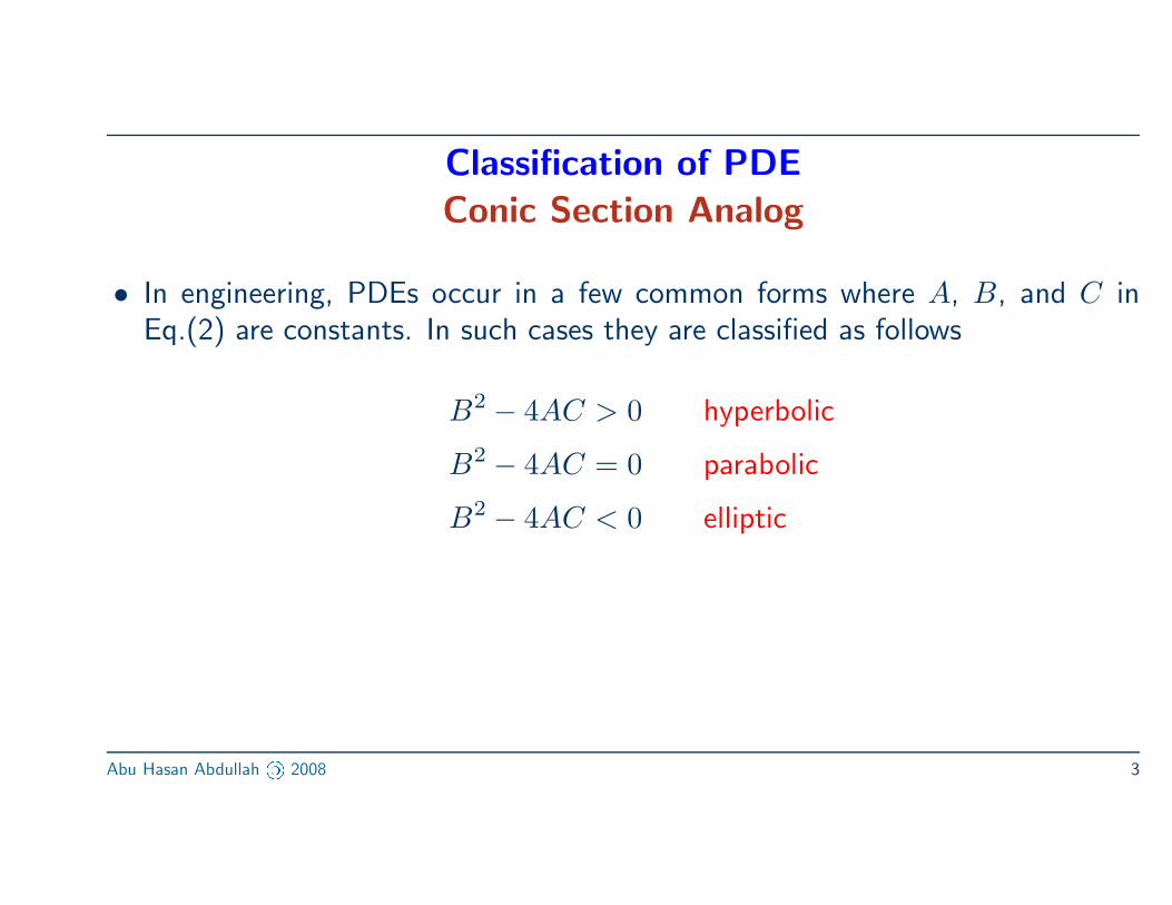
• In engineering, PDEs occur in a few common forms where A, B, and C inEq.(2) are constants. In such cases they are classified as follows

B2− 4AC > 0 hyperbolic

B2− 4AC = 0 parabolic

B2− 4AC < 0 elliptic




• In general, a PDE can have both boundary conditions (BC) and initial values(IV)

– PDEs in which only BC are specified are termed steady-state equations– PDEs in which only IV are specified are termed transient equations– PDEs in which both BC and IV are specified are termed mixed equations



Impact on Solution

• Classification of PDE leads to definition of hyperbolic, parabolic and ellipticequations

• Each type of equation has a different mathematical behaviour and this reflectsdifferent physical behaviour of flow fields

• Thus, different method should be used for solving equations associated withdifferent classification


Classic Examples of PDE

Navier-Stokes Equations

Navier-Stokes equations are PDEs governing the fluid motion and as derived, theyare of the closed-form mathematical expression.

Conservation of Mass

Dρ

Dt+ ρ∇ · V = 0 (3)




Conservation of Momentum

ρDu

Dt= −

∂p

∂x+

∂τxx

∂x+

∂τyx

∂y+

∂τzx

∂z+ ρfx (4a)

ρDv

Dt= −

∂p

∂y+

∂τxy

∂x+

∂τyy

∂y+

∂τzy

∂z+ ρfy (4b)

ρDw

Dt= −

∂p

∂z+

∂τxz

∂x+

∂τyz

∂y+

∂τzz

∂z+ ρfz (4c)




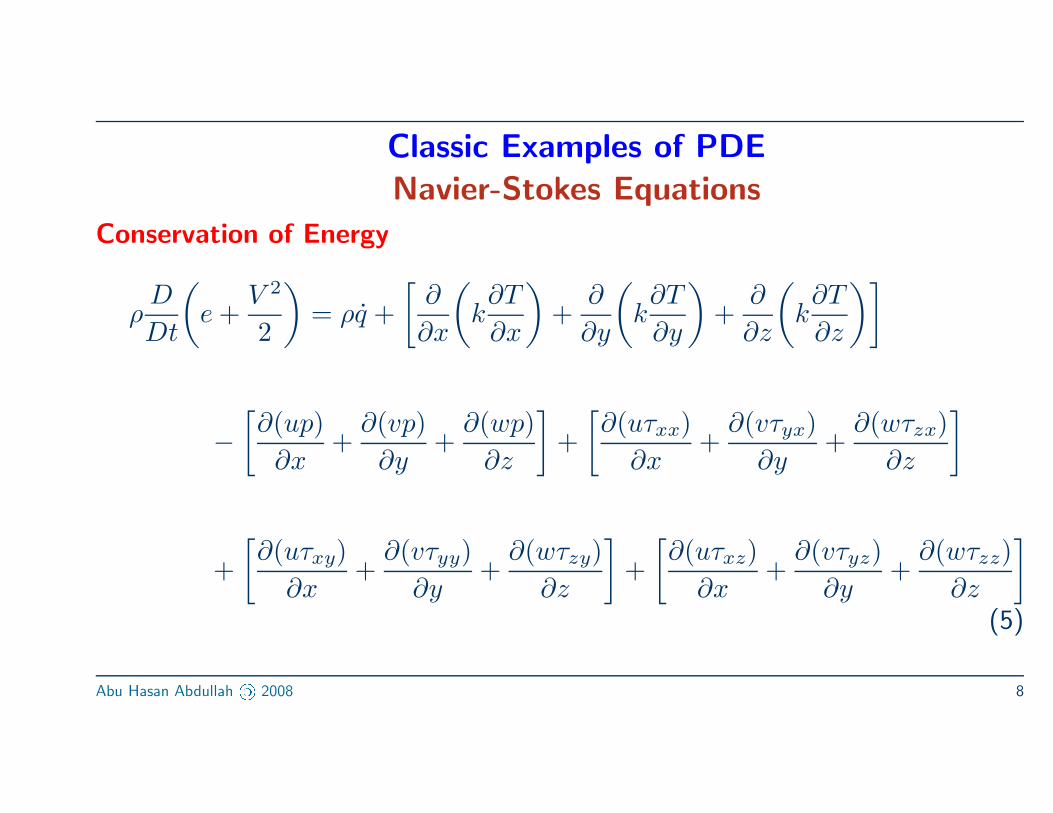
Conservation of Energy

ρD

Dt

(

e +V 2

2

)

= ρq̇ +

[∂

∂x

(

k∂T

∂x

)

+∂

∂y

(

k∂T

∂y

)

+∂

∂z

(

k∂T

∂z

)]

−

[∂(up)

∂x+

∂(vp)

∂y+

∂(wp)

∂z

]

+

[∂(uτxx)

∂x+

∂(vτyx)

∂y+

∂(wτzx)

∂z

]

+

[∂(uτxy)

∂x+

∂(vτyy)

∂y+

∂(wτzy)

∂z

]

+

[∂(uτxz)

∂x+

∂(vτyz)

∂y+

∂(wτzz)

∂z

]

(5)



Hyperbolic Navier-Stokes Equations

• Consider a hyperbolic equation of two independent variables x and y

• CFD computation of flow fields governed by hyperbolic equations is set up asmarching solutions. Algorithm is designed to start with the given initial values(IV), say the y-axis and sequentially calculate the flow field, step by step,marching in the x-direction

• Examples:

– Steady inviscid supersonic flows– Unsteady, inviscid flows



Parabolic Navier-Stokes Equations

• CFD computation of flow fields governed by parabolic equations is set up asmarching solutions. Algorithm is designed to start with the given initial values(IV), line ac and sequentially calculate the flow field, step by step, marchingin the x-direction between curves ab and cd

• Examples:

– Steady boundary-layer flows– “Parabolized” viscous flows– Unsteady thermal conduction



Elliptic Navier-Stokes Equations

• No limited regions of influence or domains of dependence. Solution at apoint is influenced by the entire closed boundary and must be carried outsimultaneously with the solution at all other points in the domain

• Also known as jury problems because the solution within the domain dependson the total boundary domain and BC must be applied over entire boundaryabcd

• Examples:

– Steady, subsonic, inviscid flow– Incompressible inviscid flow


Coordinate Transformation

• Cartesian coordinate system (x, y, z) most widely used

• Polar coordinate system very helpful in a variety of engineering problems

• Other non-standard coordinate system is also possible to cater for differentphysical orientations of the problem

• This calls for transformation of coordinate system from one form (in mostcases the cartesian) into another (polar, skewed, etc.)


Discretization

“Process by which a closed-form mathematical expression is approximatedby analogous (but different) expressions which prescribe values at only afinite number of discrete points or volumes in the domain”


Numerical Solution of PDE

• Very few analytical solutions of PDE are available. Numerical solutions

employing various numerical methods are used to overcome this limitation

• Problems governed by PDE may be classified into two categories

1. equilibrium problems (steady-state)2. marching problems (transient)



Equilibrium Problems

• Equilibrium or steady-state or jury problems are those in which a solution of agiven PDE is desired in a closed domain subject to a prescribed set of boundaryconditions

• They are boundary value problems

• Examples: steady-state temperature distributions, incompressible inviscid flows,and equilibrium stress distributions in solids

• Mathematically, they are governed by elliptic PDE



Marching Problems

• Marching or propagation problems are transient or transient-like problemswhere the solution of a PDE is required on an open domain subject to a set ofinitial conditions and a set of boundary conditions

• They are initial value or initial boundary value problems

• Solution must be computed by marching outward from initial data surfacewhile satisfying the boundary conditions

• Mathematically, they are governed by either hyperbolic or parabolic PDE



Discretization Schemes

• Various procedures using numerical methods are available

1. finite difference2. finite element3. finite volume

FINITE DIFFERENCE will be outlined



Finite Difference Method (FDM)• Physical region of problem divided into a grid of nodes, whose shape is much

influenced by nature of physical problem being solved

– structured grid reflects some type of consistent geometrical regularity– unstructured grid where grid points are located in a very irregular fashion

Coordinate transformation may take place here

• Governing PDEs transformed into corresponding coordinate system that bestfit chosen physical grid pattern, then expressed in finite difference form i.e. inthis sense, the original PDEs have been discretized!

• Finite difference form of the governing PDE applied at each of nodes, whosefunctional values are related to those nearby



Finite Difference Method (FDM)

• As a consequence of this application, a system of linear algebraic equations

developed which can be solved for unknown function values after proper BCand/or IV applied



FDM: Difference Quotients of Derivatives

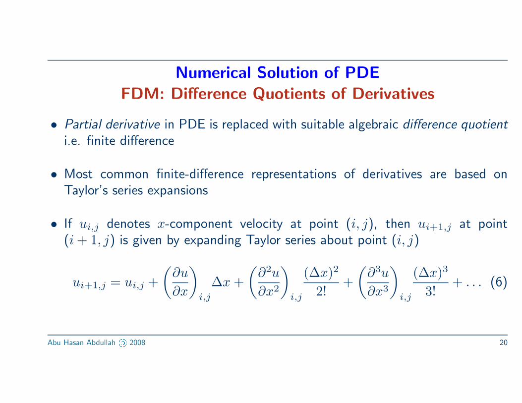
• Partial derivative in PDE is replaced with suitable algebraic difference quotient

i.e. finite difference

• Most common finite-difference representations of derivatives are based onTaylor’s series expansions

• If ui,j denotes x-component velocity at point (i, j), then ui+1,j at point(i + 1, j) is given by expanding Taylor series about point (i, j)

ui+1,j = ui,j +

(∂u

∂x

)

i,j

∆x +

(∂2u

∂x2

)

i,j

(∆x)2

2!+

(∂3u

∂x3

)

i,j

(∆x)3

3!+ . . . (6)




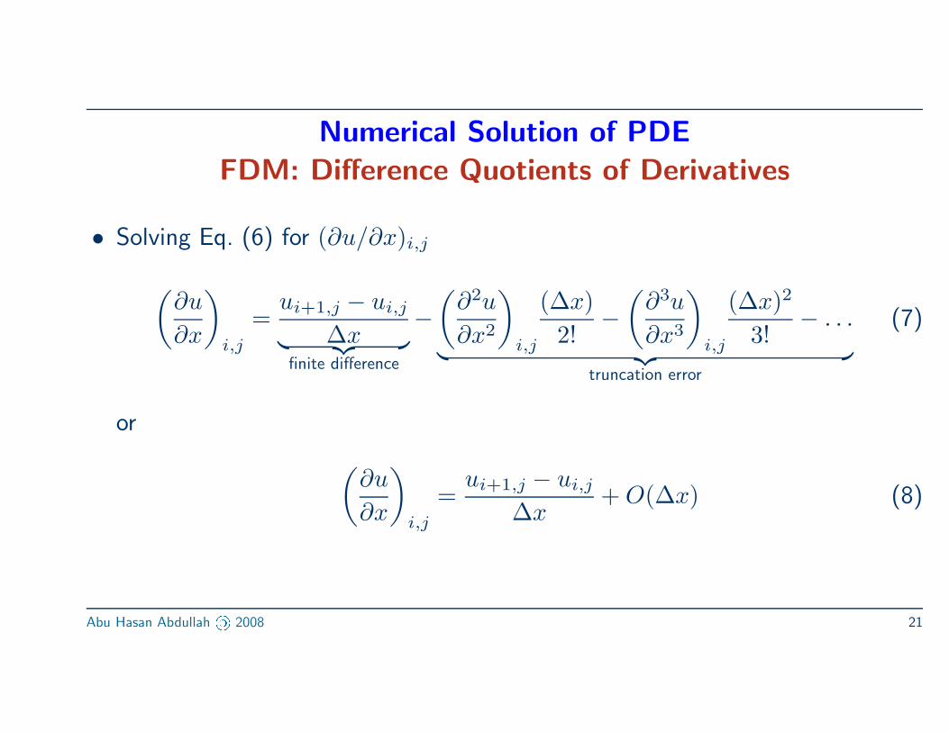
• Solving Eq. (6) for (∂u/∂x)i,j

(∂u

∂x

)

i,j

=ui+1,j − ui,j

∆x︸︷︷︸finite difference

−

(∂2u

∂x2

)

i,j

(∆x)

2!−

(∂3u

∂x3

)

i,j

(∆x)2

3!− . . .

︸︷︷︸truncation error

(7)

or

(∂u

∂x

)

i,j

=ui+1,j − ui,j

∆x+ O(∆x) (8)




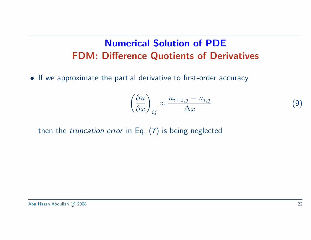
• If we approximate the partial derivative to first-order accuracy

(∂u

∂x

)

ij

≈ui+1,j − ui,j

∆x(9)

then the truncation error in Eq. (7) is being neglected




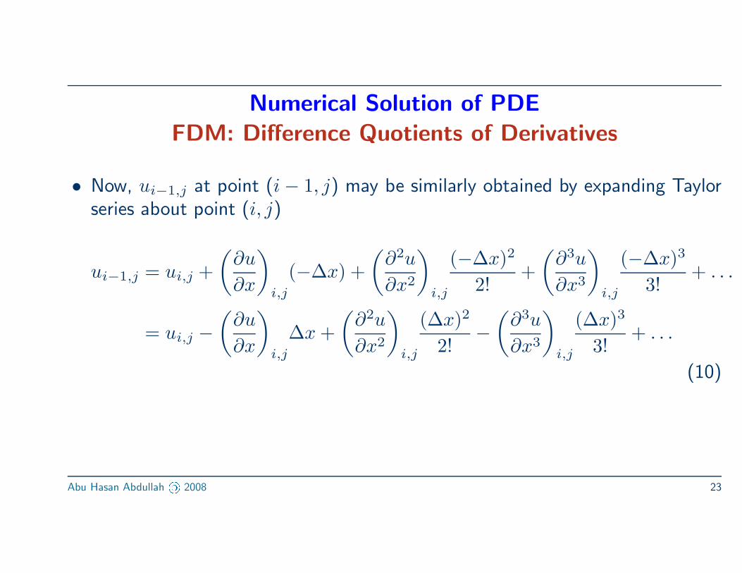
• Now, ui−1,j at point (i − 1, j) may be similarly obtained by expanding Taylorseries about point (i, j)

ui−1,j = ui,j +

(∂u

∂x

)

i,j

(−∆x) +

(∂2u

∂x2

)

i,j

(−∆x)2

2!+

(∂3u

∂x3

)

i,j

(−∆x)3

3!+ . . .

= ui,j −

(∂u

∂x

)

i,j

∆x +

(∂2u

∂x2

)

i,j

(∆x)2

2!−

(∂3u

∂x3

)

i,j

(∆x)3

3!+ . . .

(10)




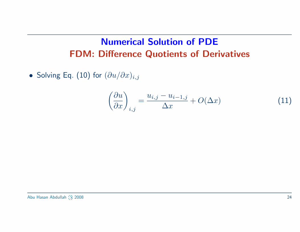
• Solving Eq. (10) for (∂u/∂x)i,j

(∂u

∂x

)

i,j

=ui,j − ui−1,j

∆x+ O(∆x) (11)




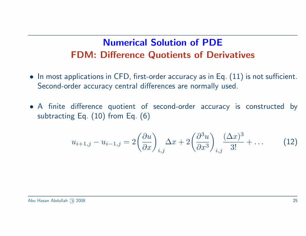
• In most applications in CFD, first-order accuracy as in Eq. (11) is not sufficient.Second-order accuracy central differences are normally used.

• A finite difference quotient of second-order accuracy is constructed bysubtracting Eq. (10) from Eq. (6)

ui+1,j − ui−1,j = 2

(∂u

∂x

)

i,j

∆x + 2

(∂3u

∂x3

)

i,j

(∆x)3

3!+ . . . (12)




• Second-order central first difference with respect to x is obtained by writingEq. (12) as

(∂u

∂x

)

i,j

=ui+1,j − ui−1,j

2∆x+ O(∆x)2 (13)

• Second-order central first difference with respect to y is obtained, throughsimilar construction, and written as

(∂u

∂y

)

i,j

=ui,j+1 − ui,j−1

2∆y+ O(∆y)2 (14)




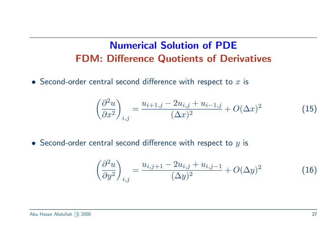
• Second-order central second difference with respect to x is

(∂2u

∂x2

)

i,j

=ui+1,j − 2ui,j + ui−1,j

(∆x)2+ O(∆x)2 (15)

• Second-order central second difference with respect to y is

(∂2u

∂y2

)

i,j

=ui,j+1 − 2ui,j + ui,j−1

(∆y)2+ O(∆y)2 (16)




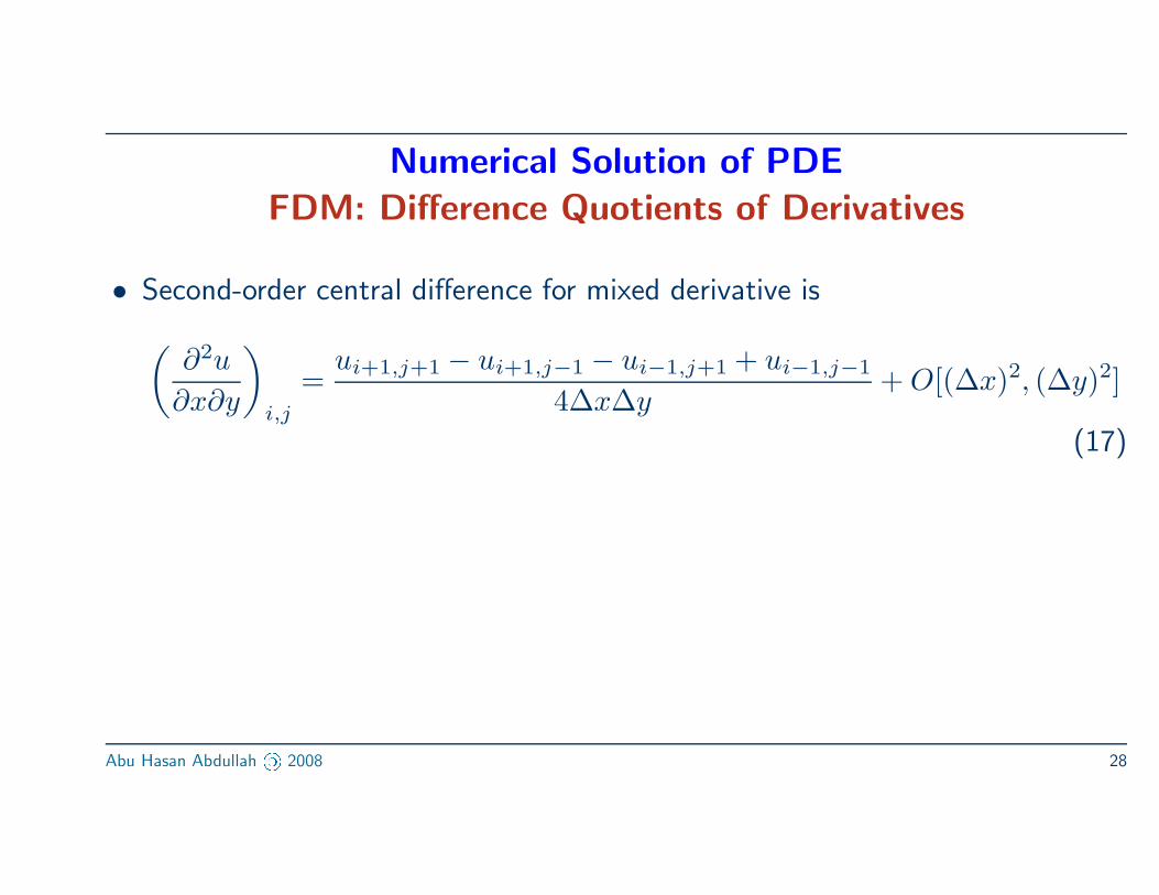
• Second-order central difference for mixed derivative is

(∂2u

∂x∂y

)

i,j

=ui+1,j+1 − ui+1,j−1 − ui−1,j+1 + ui−1,j−1

4∆x∆y+ O[(∆x)2, (∆y)2]

(17)


Using Finite Difference Method to Solve PDE

Steps

1. Physical region of problem divided into a grid of nodes, whose shape is muchinfluenced by nature of physical problem being solved, Figure 1;

• structured grid reflects some type of consistent geometrical regularity• unstructured grid where grid points are located in a very irregular fashion

2. Governing PDEs transformed into corresponding coordinate system that bestfit chosen physical grid pattern, then expressed in finite difference form i.e. inthis sense, the original PDEs have been discretized!. Coordinate transformation

may take place here


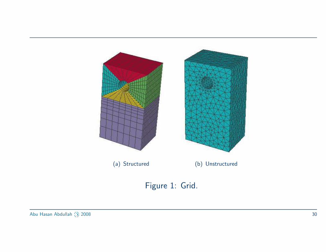
(a) Structured (b) Unstructured

Figure 1: Grid.



Steps

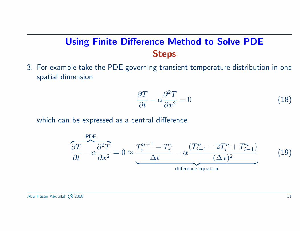
3. For example take the PDE governing transient temperature distribution in onespatial dimension

∂T

∂t− α

∂2T

∂x2= 0 (18)

which can be expressed as a central difference

PDE︷︸︸︷

∂T

∂t− α

∂2T

∂x2= 0 ≈

T n+1i − T n

i

∆t− α

(T ni+1 − 2T n

i + T ni−1)

(∆x)2︸︷︷︸

difference equation

(19)



Steps

4. The finite difference form of the governing PDE is then applied at each ofnodes, whose functional values are related to those nearby

5. As a consequence of this application, a system of linear algebraic equations

developed which can be solved for unknown function values after proper BCand/or IV applied



Coordinate Transformation

• Cartesian coordinate system (x, y, z) most widely used

• Polar coordinate system very helpful in a variety of engineering problems

• Other non-standard coordinate system is also possible to cater for differentphysical orientations of the problem

• This calls for transformation of coordinate system from one form (in mostcases the cartesian) into another (polar, skewed, etc.)

• We will cover this in greater details in the next chapter



Solution Techniques

• Difference equations formed from the discretization of PDE may be solvedusing one of these two techniques

1. explicit approach2. implicit approach

• We will use the parabolic 1-D heat conduction equation of Eq. (18)

∂T

∂t= α

∂2T

∂x2

to show differences in the two approaches



Explicit Solution Technique

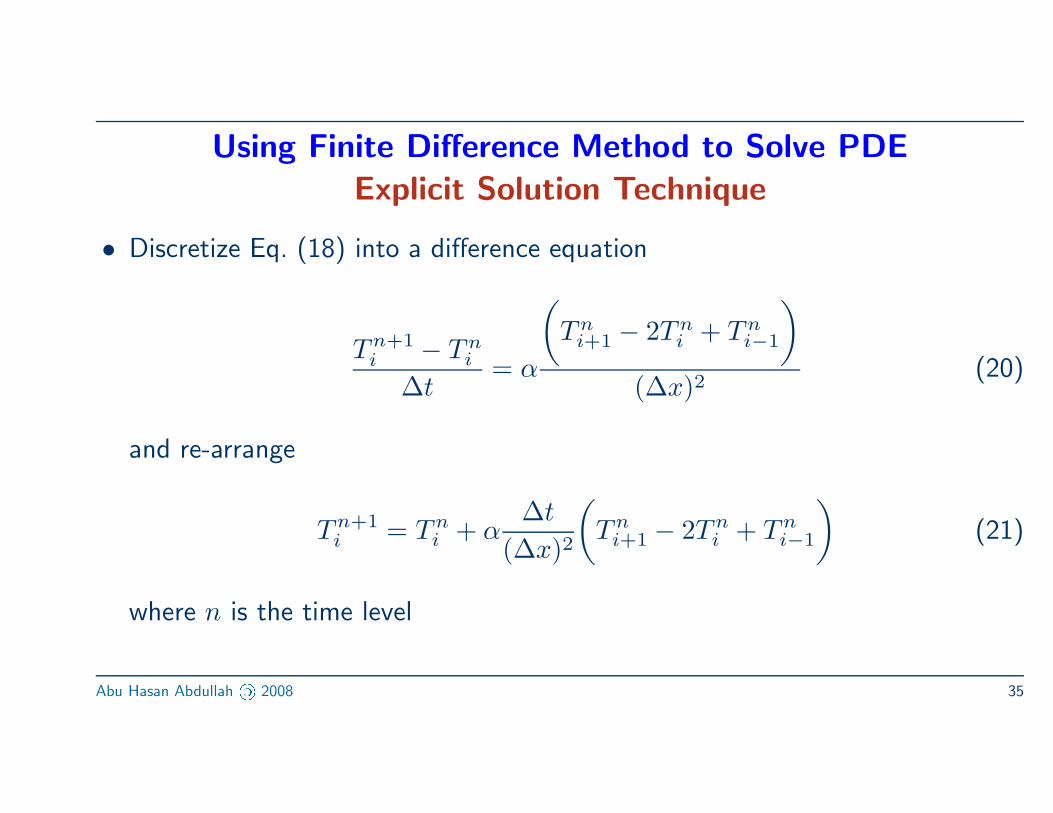
• Discretize Eq. (18) into a difference equation

T n+1i − T n

i

∆t= α

(

T ni+1 − 2T n

i + T ni−1

)

(∆x)2(20)

and re-arrange

T n+1i = T n

i + α∆t

(∆x)2

(

T ni+1 − 2T n

i + T ni−1

)

(21)

where n is the time level



Explicit Solution Technique

• In Eq. (21)

LHS = unknown properties at time level n + 1

RHS = known properties at time level n

• Eq. (21) allows direct calculation of T n+1i which is sequentially applied to all

grid points, i = 1, 2, . . . in the problem domain. This is an explicit approach

• Thus, in an explicit approach each difference equation contains only ONEunknown which can be explictly solved in a straightforward manner



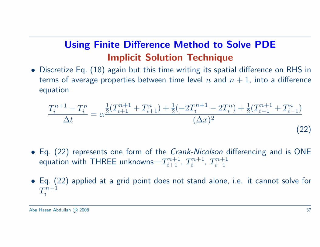
Implicit Solution Technique• Discretize Eq. (18) again but this time writing its spatial difference on RHS in

terms of average properties between time level n and n + 1, into a differenceequation

T n+1i − T n

i

∆t= α

12(T

n+1i+1 + T n

i+1) + 12(−2T n+1

i − 2T ni ) + 1

2(Tn+1i−1 + T n

i−1)

(∆x)2

(22)

• Eq. (22) represents one form of the Crank-Nicolson differencing and is ONEequation with THREE unknowns—T n+1

i+1 , T n+1i , T n+1

i−1

• Eq. (22) applied at a grid point does not stand alone, i.e. it cannot solve forT n+1

i



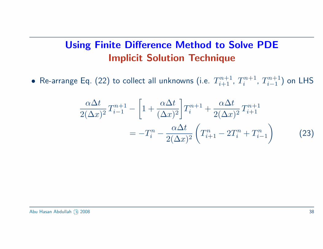
Implicit Solution Technique

• Re-arrange Eq. (22) to collect all unknowns (i.e. T n+1i+1 , T n+1

i , T n+1i−1 ) on LHS

α∆t

2(∆x)2T n+1

i−1 −

[

1 +α∆t

(∆x)2

]

T n+1i +

α∆t

2(∆x)2T n+1

i+1

= −T ni −

α∆t

2(∆x)2

(

T ni+1 − 2T n

i + T ni−1

)

(23)



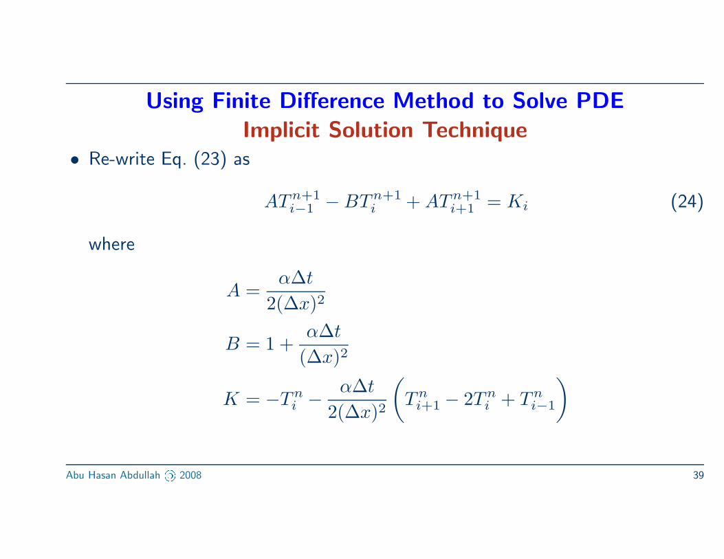
Implicit Solution Technique• Re-write Eq. (23) as

AT n+1i−1 − BT n+1

i + AT n+1i+1 = Ki (24)

where

A =α∆t

2(∆x)2

B = 1 +α∆t

(∆x)2

K = −T ni −

α∆t

2(∆x)2

(

T ni+1 − 2T n

i + T ni−1

)


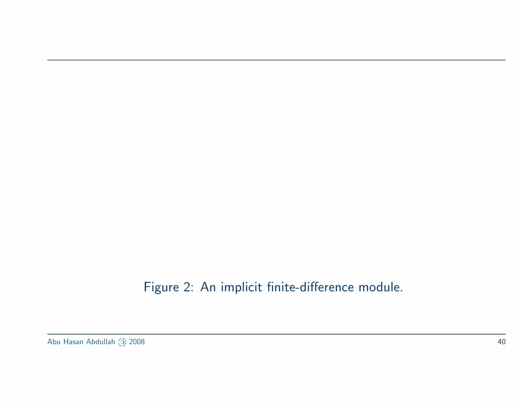
Figure 2: An implicit finite-difference module.




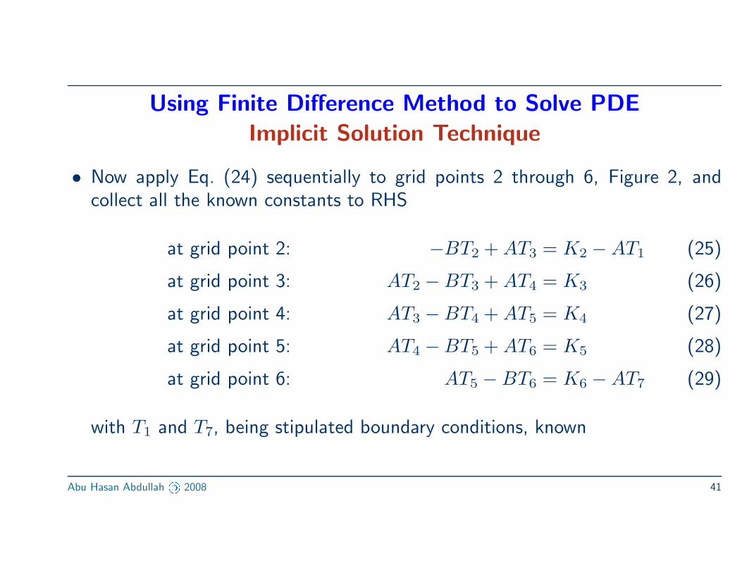
• Now apply Eq. (24) sequentially to grid points 2 through 6, Figure 2, andcollect all the known constants to RHS

at grid point 2: −BT2 + AT3 = K2 − AT1 (25)

at grid point 3: AT2 − BT3 + AT4 = K3 (26)



at grid point 6: AT5 − BT6 = K6 − AT7 (29)

with T1 and T7, being stipulated boundary conditions, known




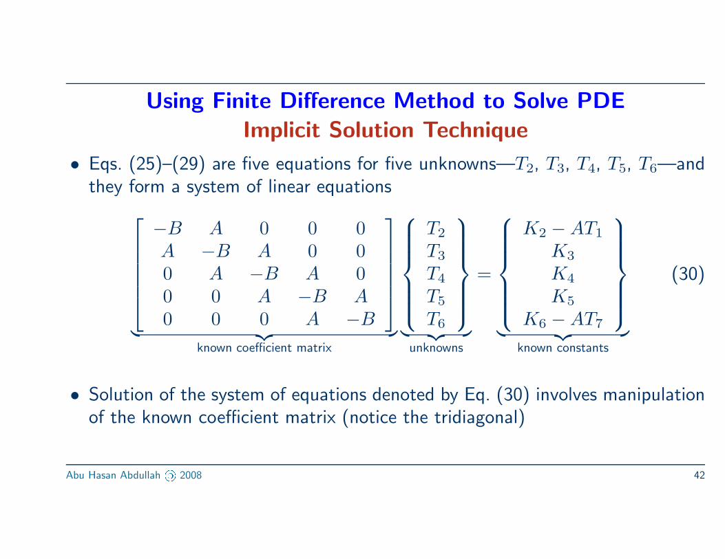
• Eqs. (25)–(29) are five equations for five unknowns—T2, T3, T4, T5, T6—andthey form a system of linear equations

−B A 0 0 0A −B A 0 00 A −B A 00 0 A −B A0 0 0 A −B

︸︷︷︸known coefficient matrix

T2

T3

T4

T5

T6

︸︷︷︸unknowns

=

K2 − AT1

K3

K4

K5

K6 − AT7

︸︷︷︸known constants

(30)

• Solution of the system of equations denoted by Eq. (30) involves manipulationof the known coefficient matrix (notice the tridiagonal)


Homeworks

Read through Chapter 4 of Computational Fluid Dynamics (1995), Anderson,

J.D. and discuss briefly the meaning of

1. structured grids

2. unstructured grids

3. first-order-accurate finite-difference expression

4. second-order-accurate finite-difference expression

5. truncation error and its influence on your CFD calculation


HomeworksUsing central-difference approximations, find the solution of the wave equation, represented by a

second-order hyperbolic equation:

∂2φ

∂x=

∂2φ

∂t2, 0 ≤ x ≤ 1

subject to the boundary conditions

φ(0, t) = 0 t > 0

φ(1, t) = 0 t > 0

and initial conditions

φ(x, 0) = sin πx 0 ≤ x ≤ 1

∂φ

∂t(x, 0) = 0 0 ≤ x ≤ 1


Figure 3: 2-D finite difference discretization


applied numerical methods partial diﬀerential...

Documents