applied multivariate analysis - research-training.net · applied multivariate analysis adam smith...
TRANSCRIPT

Applied Multivariate Analysis
Adam Smith Business SchoolGlasgow University
February 25–28, 2019
Generalized linear models: a generic approach to
statistical analysis
www.research-training.net/Glasgow
University of Manchester
Graeme Hutcheson Applied Multivariate Analysis

The slides and R-files for this session are available for downloadfrom the course website...
www.research-training.net/Glasgow
Graeme Hutcheson Applied Multivariate Analysis
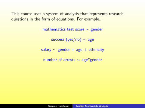
This course uses a system of analysis that represents researchquestions in the form of equations. For example...
mathematics test score ∼ gender
success (yes/no) ∼ age
salary ∼ gender + age + ethnicity
number of arrests ∼ age*gender
Representing research questions in this way explicitly identifies therelationships to be tested, the structure of the data and how themodel is entered into the analysis programme.
Graeme Hutcheson Applied Multivariate Analysis
The formulation of the research question in equation format is alsouseful as it is the same representation as that used by theGeneralized Linear Model (GLM); a statistical model that may beapplied to a range of analytical problems.
This lecture provides a relatively non-technical introduction to theGLM. Those looking for more detailed treatments are advised tolook at the following texts...
McCullagh, P. and Nelder, J. A. (1989). Generalized Linear Models(2nd edition). Chapman & Hall/CRC.
Hutcheson, G. D. and Sofroniou, N. (1999). The MultivariateSocial Scientist: Introductory statistics using generalizedlinear models. Sage Publications.
Graeme Hutcheson Applied Multivariate Analysis
The Generalized Linear Model
In it’s simplest form, the GLM is a statistical technique thatpredicts a single variable (the response variable), using one or moreother variables (the explanatory variables).
The response and explanatory variables (also known as the randomand systematic components of the model) are linked (∼) accordingto a function that takes account of the measurement scale of theresponse variable.
response variable ∼ explanatory variables
There are many link functions that are available for GLM modelsto take account of the different ways in which the randomcomponent (the variable that is being predicted) is distributed (eg.as a number, category, count, skewed, etc.). This courseintroduces three links that enable continuous, categorical andcount response variables to be modelled.
Graeme Hutcheson Applied Multivariate Analysis
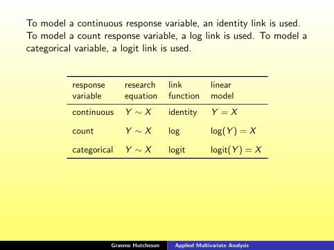
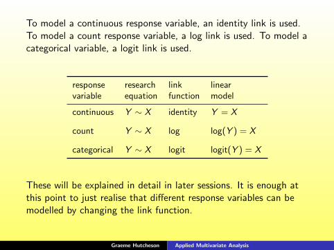
To model a continuous response variable, an identity link is used.To model a count response variable, a log link is used. To model acategorical variable, a logit link is used.
response research link linearvariable equation function model
continuous Y ∼ X identity Y = X
count Y ∼ X log log(Y ) = X
categorical Y ∼ X logit logit(Y ) = X
These will be explained in detail in later sessions. It is enough atthis point to just realise that different response variables can bemodelled by changing the link function.
Graeme Hutcheson Applied Multivariate Analysis
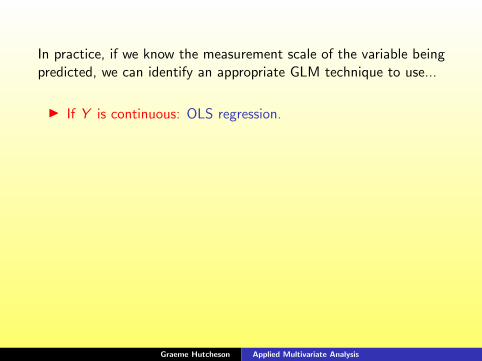
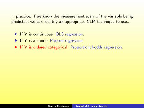
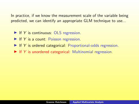
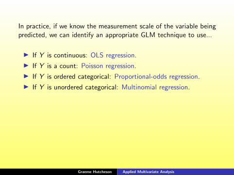
In practice, if we know the measurement scale of the variable beingpredicted, we can identify an appropriate GLM technique to use...
I If Y is continuous: OLS regression.
I If Y is a count: Poisson regression.
I If Y is ordered categorical: Proportional-odds regression.
I If Y is unordered categorical: Multinomial regression.
GLM models are particularly powerful, as they are all conceptuallyvery similar. Learning to apply and interpret results from onetechnique greatly helps in applying and interpreting results fromthe others.
Graeme Hutcheson Applied Multivariate Analysis

GLM — a statistical representation
Up till now models have been represented using variable names.This way of looking at models is very useful as it is the way thatmodels are conceptualised and input into the statistical software.
It is useful, however, to also represent models using a moredetailed statistical representation; one that corresponds to the waythat the results are produced and reported.
The statistical representation simply includes some parameters thatquantify the relationships in the data. We not only want to knowthat Y and X are related, we also want to know HOW they arerelated. ie. When X changes by a set amount, what is the effecton Y ?
Graeme Hutcheson Applied Multivariate Analysis

GLM — the parameters
A conceptual model of ice cream consumption (from the IceCream
dataset) is...
consumption ∼ temperature
which is represented statistically as...
consumption = β0 + β1 temperature
where
β0 estimates ‘consumption’ when ‘temperature’ is zero.
β1 estimates the change in ‘consumption’ for a unit increase in‘temperature’.
Graeme Hutcheson Applied Multivariate Analysis
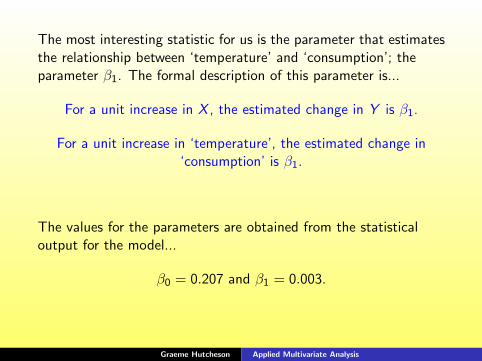
The most interesting statistic for us is the parameter that estimatesthe relationship between ‘temperature’ and ‘consumption’; theparameter β1. The formal description of this parameter is...
For a unit increase in X , the estimated change in Y is β1.
For a unit increase in ‘temperature’, the estimated change in‘consumption’ is β1.
The values for the parameters are obtained from the statisticaloutput for the model...
β0 = 0.207 and β1 = 0.003.
Graeme Hutcheson Applied Multivariate Analysis
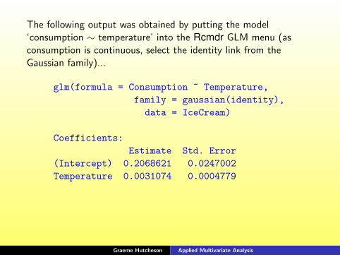
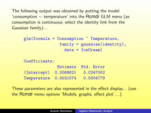
The following output was obtained by putting the model‘consumption ∼ temperature’ into the Rcmdr GLM menu (asconsumption is continuous, select the identity link from theGaussian family)...
glm(formula = Consumption ~ Temperature,
family = gaussian(identity),
data = IceCream)
Coefficients:
Estimate Std. Error
(Intercept) 0.2068621 0.0247002
Temperature 0.0031074 0.0004779
These parameters are also represented in the effect display... (usethe Rcmdr menu options ‘Models, graphs, effect plot’....).
Graeme Hutcheson Applied Multivariate Analysis
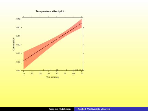
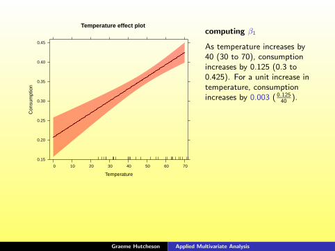
Temperature effect plot
Temperature
Con
sum
ptio
n
0.15
0.20
0.25
0.30
0.35
0.40
0.45
0 10 20 30 40 50 60 70
computing β1
As temperature increases by40 (30 to 70), consumptionincreases by 0.125 (0.3 to0.425). For a unit increase intemperature, consumptionincreases by 0.003 ( 0.125
40).
computing β0
The value of ‘consumption’when ‘temperature’ = 0. Asimple estimation from thegraph shows β0 = 0.2.
Graeme Hutcheson Applied Multivariate Analysis

Categorical explanatory variables...
It is useful at this stage to look at categorical explanatoryvariables. A detailed description of analysing categoricalexplanatory variables is available in...
Hutcheson, G. D. (2011). Categorical Explanatory Variables.Journal of Modelling in Management. 6, 2: 225–236.
At a basic level, categorical variables are divided into a number ofbinary comparisons. Each category is then compared to a specificcategory (the reference).
The following slide shows a model of examination score andwhether this is related to the school a child is at. school is anunordered categorical variable with three categories (schoolA,schoolB and schoolC).
Graeme Hutcheson Applied Multivariate Analysis
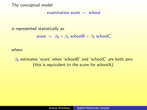
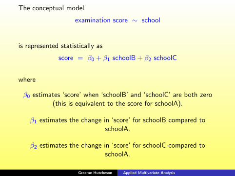
The conceptual model
examination score ∼ school
is represented statistically as
score = β0 + β1 schoolB + β2 schoolC
where
β0 estimates ‘score’ when ‘schoolB’ and ‘schoolC’ are both zero(this is equivalent to the score for schoolA).
β1 estimates the change in ‘score’ for schoolB compared toschoolA.
β2 estimates the change in ‘score’ for schoolC compared toschoolA.
Graeme Hutcheson Applied Multivariate Analysis
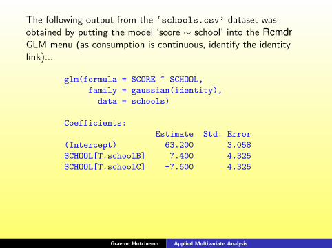
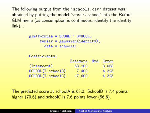
The following output from the ‘schools.csv’ dataset wasobtained by putting the model ‘score ∼ school’ into the RcmdrGLM menu (as consumption is continuous, identify the identitylink)...
glm(formula = SCORE ~ SCHOOL,
family = gaussian(identity),
data = schools)
Coefficients:
Estimate Std. Error
(Intercept) 63.200 3.058
SCHOOL[T.schoolB] 7.400 4.325
SCHOOL[T.schoolC] -7.600 4.325
The predicted score at schoolA is 63.2. SchoolB is 7.4 pointshigher (70.6) and schoolC is 7.6 points lower (56.6).
Graeme Hutcheson Applied Multivariate Analysis
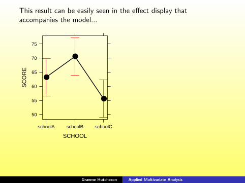
This result can be easily seen in the effect display thataccompanies the model...
SCHOOL
SC
OR
E
50
55
60
65
70
75
schoolA schoolB schoolC
●
●
●
β0 = 63.2
The value of ‘score’ for‘schoolA’ (the referencecategory).
β1 = 70.6
schoolB is 7.4 units higher thanschoolA.
β2 = 56.6
schoolC is 7.6 units lower thanschoolA.
Graeme Hutcheson Applied Multivariate Analysis
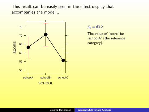
This result can be easily seen in the effect display thataccompanies the model...
SCHOOL
SC
OR
E
50
55
60
65
70
75
schoolA schoolB schoolC
●
●
●
β0 = 63.2
The value of ‘score’ for‘schoolA’ (the referencecategory).
β1 = 70.6
schoolB is 7.4 units higher thanschoolA.
β2 = 56.6
schoolC is 7.6 units lower thanschoolA.
Graeme Hutcheson Applied Multivariate Analysis
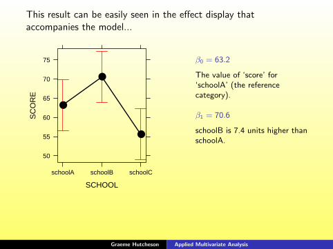
This result can be easily seen in the effect display thataccompanies the model...
SCHOOL
SC
OR
E
50
55
60
65
70
75
schoolA schoolB schoolC
●
●
●
β0 = 63.2
The value of ‘score’ for‘schoolA’ (the referencecategory).
β1 = 70.6
schoolB is 7.4 units higher thanschoolA.
β2 = 56.6
schoolC is 7.6 units lower thanschoolA.
Graeme Hutcheson Applied Multivariate Analysis
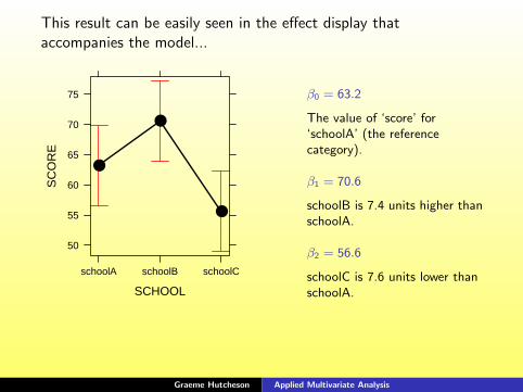
This result can be easily seen in the effect display thataccompanies the model...
SCHOOL
SC
OR
E
50
55
60
65
70
75
schoolA schoolB schoolC
●
●
●
β0 = 63.2
The value of ‘score’ for‘schoolA’ (the referencecategory).
β1 = 70.6
schoolB is 7.4 units higher thanschoolA.
β2 = 56.6
schoolC is 7.6 units lower thanschoolA.
Graeme Hutcheson Applied Multivariate Analysis
interpreting parameters for other GLMs
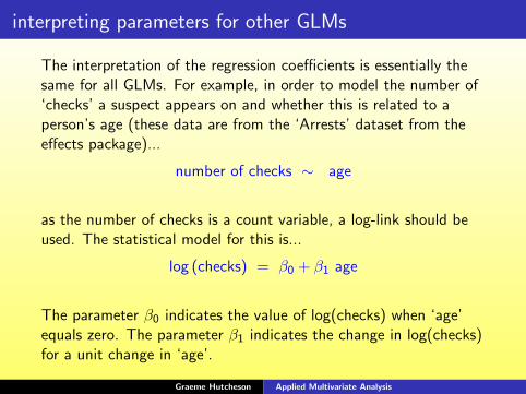
The interpretation of the regression coefficients is essentially thesame for all GLMs. For example, in order to model the number of‘checks’ a suspect appears on and whether this is related to aperson’s age (these data are from the ‘Arrests’ dataset from theeffects package)...
number of checks ∼ age
as the number of checks is a count variable, a log-link should beused. The statistical model for this is...
log (checks) = β0 + β1 age
The parameter β0 indicates the value of log(checks) when ‘age’equals zero. The parameter β1 indicates the change in log(checks)for a unit change in ‘age’.
Graeme Hutcheson Applied Multivariate Analysis

interpreting parameters for other GLMs
The interpretation of the regression coefficients is essentially thesame for all GLMs. For example, in order to model the number of‘checks’ a suspect appears on and whether this is related to aperson’s age (these data are from the ‘Arrests’ dataset from theeffects package)...
number of checks ∼ age
as the number of checks is a count variable, a log-link should beused. The statistical model for this is...
log (checks) = β0 + β1 age
The parameter β0 indicates the value of log(checks) when ‘age’equals zero. The parameter β1 indicates the change in log(checks)for a unit change in ‘age’.
Graeme Hutcheson Applied Multivariate Analysis
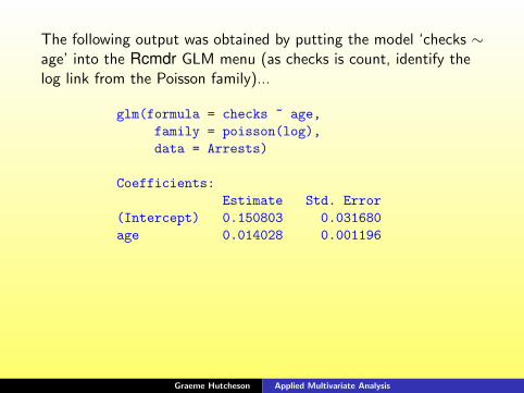
The following output was obtained by putting the model ‘checks ∼age’ into the Rcmdr GLM menu (as checks is count, identify thelog link from the Poisson family)...
glm(formula = checks ~ age,
family = poisson(log),
data = Arrests)
Coefficients:
Estimate Std. Error
(Intercept) 0.150803 0.031680
age 0.014028 0.001196
When ‘age’ = 0, ‘log(count)’ = 0.151.
For a unit increase in ‘age’, ‘log(count)’ changes by 0.014.
Graeme Hutcheson Applied Multivariate Analysis

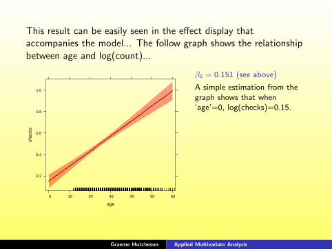
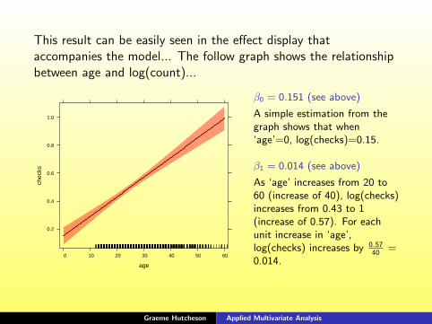
This result can be easily seen in the effect display thataccompanies the model... The follow graph shows the relationshipbetween age and log(count)...
age
chec
ks
0.2
0.4
0.6
0.8
1.0
0 10 20 30 40 50 60
β0 = 0.151 (see above)
A simple estimation from thegraph shows that when‘age’=0, log(checks)=0.15.
β1 = 0.014 (see above)
As ‘age’ increases from 20 to60 (increase of 40), log(checks)increases from 0.43 to 1(increase of 0.57). For eachunit increase in ‘age’,log(checks) increases by 0.57
40=
0.014.
Graeme Hutcheson Applied Multivariate Analysis
The model parameters for GLM models have an easyinterpretation; one that is essentially the same for all GLM models.
The parameters can be interpreted from the ‘standard’ statisticaloutput shown in the tables, or from the effect displays.
Graeme Hutcheson Applied Multivariate Analysis
The model parameters for GLM models have an easyinterpretation; one that is essentially the same for all GLM models.
The parameters can be interpreted from the ‘standard’ statisticaloutput shown in the tables, or from the effect displays.
Graeme Hutcheson Applied Multivariate Analysis

Assessing significance...
Graeme Hutcheson Applied Multivariate Analysis

Assessing significance for GLMs
In order to interpret the models, it is useful to know thesignificance associated with each of the parameter estimates.Although ‘consumption’ may increase by 0.003 for each unitincrease in ‘temperature’; there is no indication whether thisincrease may have been due to chance.
In addition to the parameter estimates, we usually also want toknow which parameters, or groups of parameters are significant.
This is where the GLM models excel, as they employ a simplemethod for determining significance; one that applies generally toall GLMs.
Graeme Hutcheson Applied Multivariate Analysis
Deviance
Significance is assessed in GLMs using a common method based ona statistic known as the deviance.
The deviance is simply a measure of the difference between thevalues predicted by the model and the actual values (predictedvalues compared to the observed data). If the model provides agood prediction of the response variable, the deviance will berelatively small. If the model does not provide accurate predictionsof the response variable, the deviance will be relatively large.
The deviance basically gives an indication of how well the modelfits the data.
Graeme Hutcheson Applied Multivariate Analysis
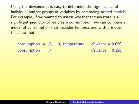
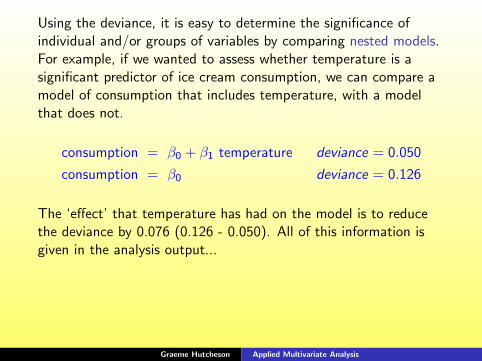
Using the deviance, it is easy to determine the significance ofindividual and/or groups of variables by comparing nested models.For example, if we wanted to assess whether temperature is asignificant predictor of ice cream consumption, we can compare amodel of consumption that includes temperature, with a modelthat does not.
consumption = β0 + β1 temperature deviance = 0.050
consumption = β0 deviance = 0.126
The ‘effect’ that temperature has had on the model is to reducethe deviance by 0.076 (0.126 - 0.050). All of this information isgiven in the analysis output...
The Null deviance is the deviance in the response variable withouttaking into account any other information. The Residual devianceis the deviance in the model that includes the explanatory variables.
Graeme Hutcheson Applied Multivariate Analysis

glm(formula = Consumption ~ Temperature,
family = gaussian(identity), data = IceCream)
Coefficients:
Estimate Std. Error t value Pr(>|t|)
(Intercept) 0.2068621 0.0247002 8.375 4.13e-09
Temperature 0.0031074 0.0004779 6.502 4.79e-07
Null deviance: 0.125523 on 29 degrees of freedom
Residual deviance: 0.050009 on 28 degrees of freedom
Analysis of Deviance Table (Type II tests)
Response: Consumption
SS Df F Pr(>F)
Temperature 0.075514 1 42.28 4.789e-07
Residuals 0.050009 28
Graeme Hutcheson Applied Multivariate Analysis
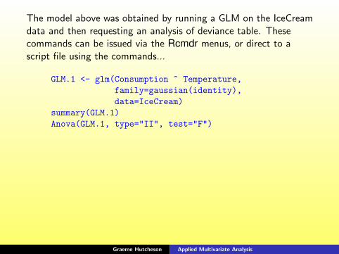
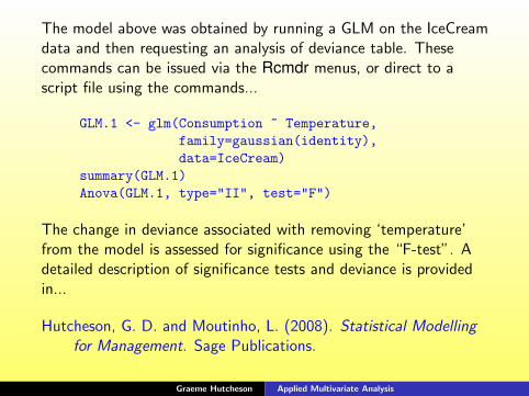
The model above was obtained by running a GLM on the IceCreamdata and then requesting an analysis of deviance table. Thesecommands can be issued via the Rcmdr menus, or direct to ascript file using the commands...
GLM.1 <- glm(Consumption ~ Temperature,
family=gaussian(identity),
data=IceCream)
summary(GLM.1)
Anova(GLM.1, type="II", test="F")
The change in deviance associated with removing ‘temperature’from the model is assessed for significance using the “F-test”. Adetailed description of significance tests and deviance is providedin...
Hutcheson, G. D. and Moutinho, L. (2008). Statistical Modellingfor Management. Sage Publications.
Graeme Hutcheson Applied Multivariate Analysis

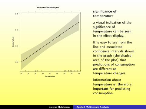
Temperature effect plot
Temperature
Con
sum
ptio
n
0.30
0.35
0.40
0.45
30 35 40 45 50 55 60 65 70
significance oftemperature
a visual indication of thesignificance oftemperature can be seenin the effect display.
It is easy to see from theline and associatedconfidence intervals shownin the graph (the shadedarea of the plot) thatpredictions of consumptionare different astemperature changes.
Information abouttemperature is, therefore,important for predictingconsumption.
Graeme Hutcheson Applied Multivariate Analysis

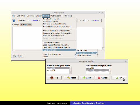
The significance of temperature in the model can be manuallycalculated by comparing the nested models...
model01: consumption = β0
model02: consumption = β0 + β1 temperature
This can be easily achieved using the Rcmdr Models, Hypothesistests, Compare two models... menu option.
Graeme Hutcheson Applied Multivariate Analysis
Graeme Hutcheson Applied Multivariate Analysis
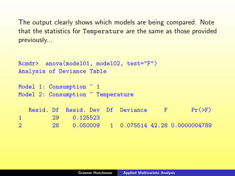
The output clearly shows which models are being compared. Notethat the statistics for Temperature are the same as those providedpreviously...
Rcmdr> anova(model01, model02, test="F")
Analysis of Deviance Table
Model 1: Consumption ~ 1
Model 2: Consumption ~ Temperature
Resid. Df Resid. Dev Df Deviance F Pr(>F)
1 29 0.125523
2 28 0.050009 1 0.075514 42.28 0.0000004789
Graeme Hutcheson Applied Multivariate Analysis

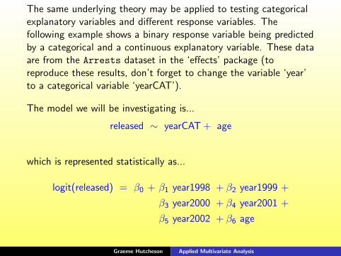
The same underlying theory may be applied to testing categoricalexplanatory variables and different response variables. Thefollowing example shows a binary response variable being predictedby a categorical and a continuous explanatory variable. These dataare from the Arrests dataset in the ‘effects’ package (toreproduce these results, don’t forget to change the variable ‘year’to a categorical variable ‘yearCAT’).
The model we will be investigating is...
released ∼ yearCAT + age
which is represented statistically as...
logit(released) = β0 + β1 year1998 + β2 year1999 +
β3 year2000 + β4 year2001 +
β5 year2002 + β6 age
Graeme Hutcheson Applied Multivariate Analysis

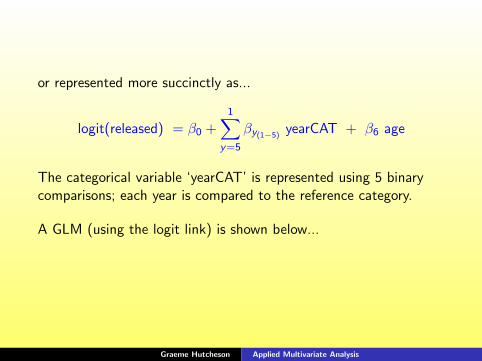
or represented more succinctly as...
logit(released) = β0 +1∑
y=5
βy(1−5)yearCAT + β6 age
The categorical variable ‘yearCAT’ is represented using 5 binarycomparisons; each year is compared to the reference category.
A GLM (using the logit link) is shown below...
Graeme Hutcheson Applied Multivariate Analysis
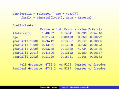
glm(formula = released ~ age + yearCAT,
family = binomial(logit), data = Arrests)
Coefficients:
Estimate Std. Error z value Pr(>|z|)
(Intercept) 1.48937 0.14841 10.036 < 2e-16
age -0.01294 0.00423 -3.059 0.00222
yearCAT[T.1998] 0.36712 0.13857 2.649 0.00806
yearCAT[T.1999] 0.43182 0.13360 3.232 0.00123
yearCAT[T.2000] 0.63258 0.13362 4.734 2.2e-06
yearCAT[T.2001] 0.41696 0.13112 3.180 0.00147
yearCAT[T.2002] 0.21149 0.18451 1.146 0.25172
Null deviance: 4776.3 on 5225 degrees of freedom
Residual deviance: 4743.2 on 5219 degrees of freedom
Graeme Hutcheson Applied Multivariate Analysis
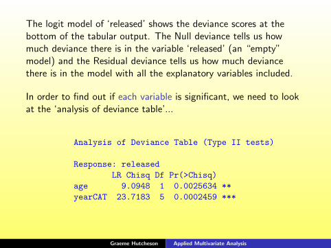
The logit model of ‘released’ shows the deviance scores at thebottom of the tabular output. The Null deviance tells us howmuch deviance there is in the variable ‘released’ (an “empty”model) and the Residual deviance tells us how much deviancethere is in the model with all the explanatory variables included.
In order to find out if each variable is significant, we need to lookat the ‘analysis of deviance table’...
Analysis of Deviance Table (Type II tests)
Response: released
LR Chisq Df Pr(>Chisq)
age 9.0948 1 0.0025634 **
yearCAT 23.7183 5 0.0002459 ***
Graeme Hutcheson Applied Multivariate Analysis

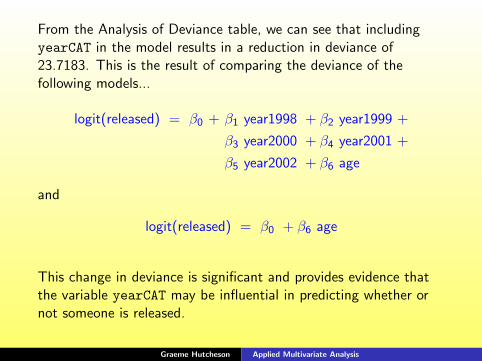
From the Analysis of Deviance table, we can see that includingyearCAT in the model results in a reduction in deviance of23.7183. This is the result of comparing the deviance of thefollowing models...
logit(released) = β0 + β1 year1998 + β2 year1999 +
β3 year2000 + β4 year2001 +
β5 year2002 + β6 age
and
logit(released) = β0 + β6 age
This change in deviance is significant and provides evidence thatthe variable yearCAT may be influential in predicting whether ornot someone is released.
Graeme Hutcheson Applied Multivariate Analysis
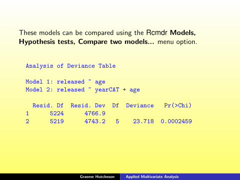
These models can be compared using the Rcmdr Models,Hypothesis tests, Compare two models... menu option.
Analysis of Deviance Table
Model 1: released ~ age
Model 2: released ~ yearCAT + age
Resid. Df Resid. Dev Df Deviance Pr(>Chi)
1 5224 4766.9
2 5219 4743.2 5 23.718 0.0002459
Graeme Hutcheson Applied Multivariate Analysis
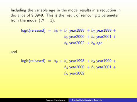
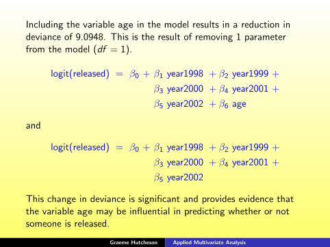
Including the variable age in the model results in a reduction indeviance of 9.0948. This is the result of removing 1 parameterfrom the model (df = 1).
logit(released) = β0 + β1 year1998 + β2 year1999 +
β3 year2000 + β4 year2001 +
β5 year2002 + β6 age
and
logit(released) = β0 + β1 year1998 + β2 year1999 +
β3 year2000 + β4 year2001 +
β5 year2002
This change in deviance is significant and provides evidence thatthe variable age may be influential in predicting whether or notsomeone is released.
Graeme Hutcheson Applied Multivariate Analysis
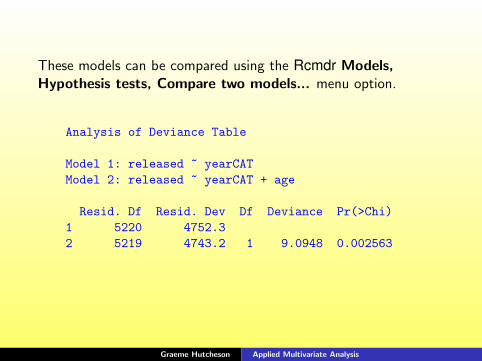
These models can be compared using the Rcmdr Models,Hypothesis tests, Compare two models... menu option.
Analysis of Deviance Table
Model 1: released ~ yearCAT
Model 2: released ~ yearCAT + age
Resid. Df Resid. Dev Df Deviance Pr(>Chi)
1 5220 4752.3
2 5219 4743.2 1 9.0948 0.002563
Graeme Hutcheson Applied Multivariate Analysis
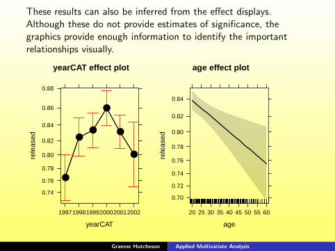
These results can also be inferred from the effect displays.Although these do not provide estimates of significance, thegraphics provide enough information to identify the importantrelationships visually.
yearCAT effect plot
yearCAT
rele
ased
0.74
0.76
0.78
0.80
0.82
0.84
0.86
0.88
199719981999200020012002
●
●●
●
●
●
age effect plot
age
rele
ased
0.70
0.72
0.74
0.76
0.78
0.80
0.82
0.84
20 25 30 35 40 45 50 55 60
Graeme Hutcheson Applied Multivariate Analysis
The significance of each category to the prediction of the responsevariable in logit models is estimated using the z-distribution in the‘standard’ regression output. It should be noted that this is alarge-sample approximation and the deviance statistic is preferablefor assessing significance. Full information about this is availablein...
Hutcheson, G. D. and Moutinho, L. (2008). Statistical Modelling forManagement. Sage Publications.
Graeme Hutcheson Applied Multivariate Analysis

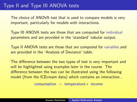
Type II and Type III ANOVA tests
The choice of ANOVA test that is used to compare models is veryimportant, particularly for models with interactions.
Type III ANOVA tests are those that are computed for individualparameters and are provided in the ‘standard’ tabular output.
Type II ANOVA tests are those that are computed for variables andare provided in the ‘Analysis of Deviance’ table.
The difference between the two types of test is very important andwill be highlighted using examples later in the course. Thedifference between the two can be illustrated using the followingmodel (from the ICEcream data) which contains an interaction...
consumption ∼ temperature ∗ income
Graeme Hutcheson Applied Multivariate Analysis
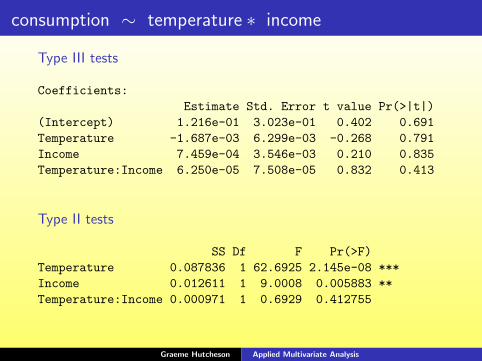
consumption ∼ temperature ∗ income
Type III tests
Coefficients:
Estimate Std. Error t value Pr(>|t|)
(Intercept) 1.216e-01 3.023e-01 0.402 0.691
Temperature -1.687e-03 6.299e-03 -0.268 0.791
Income 7.459e-04 3.546e-03 0.210 0.835
Temperature:Income 6.250e-05 7.508e-05 0.832 0.413
Type II tests
SS Df F Pr(>F)
Temperature 0.087836 1 62.6925 2.145e-08 ***
Income 0.012611 1 9.0008 0.005883 **
Temperature:Income 0.000971 1 0.6929 0.412755
Graeme Hutcheson Applied Multivariate Analysis
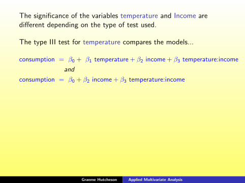
The significance of the variables temperature and Income aredifferent depending on the type of test used.
The type III test for temperature compares the models...
consumption = β0 + β1 temperature + β2 income + β3 temperature:income
and
consumption = β0 + β2 income + β3 temperature:income
whilst the type II test for temperature compares the models...
consumption = β0 + β1 temperature + β2 income
and
consumption = β0 + β2 income
Graeme Hutcheson Applied Multivariate Analysis
The type III test does not provide an indication of the significanceof the variable temperature. We need to compare a model thatincludes temperature with a model thatdoes not - BOTH of thesemodesl include temperature.
The type II test does compare models differentiated on the basis oftemperature and are, therefore, more appropriate for assessing theeffect of temperature.
Graeme Hutcheson Applied Multivariate Analysis

Traditional tests andequivalent GLM models...
Graeme Hutcheson Applied Multivariate Analysis
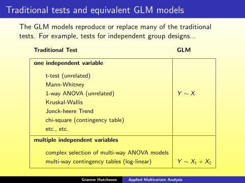
Traditional tests and equivalent GLM models
The GLM models reproduce or replace many of the traditionaltests. For example, tests for independent group designs...
Traditional Test GLM
one independent variable
t-test (unrelated)
Mann-Whitney
1-way ANOVA (unrelated) Y ∼ X
Kruskal-Wallis
Jonck-heere Trend
chi-square (contingency table)
etc., etc.
multiple independent variables
complex selection of multi-way ANOVA models
multi-way contingency tables (log-linear) Y ∼ X1 + X2
Graeme Hutcheson Applied Multivariate Analysis

Traditional tests and equivalent GLM models
... and tests for dependent (or matched) group designs...
Traditional Test GLM
one independent variable
paired t-test
Wilcoxon
1-way ANOVA (related) Y ∼ subject + X
Friedman
Pages L-trend
etc., etc.,
multiple independent variables
complex selection of multi-way ANOVA models
multi-way contingency tables (log-linear) Y ∼ subject + X1 + X2
Graeme Hutcheson Applied Multivariate Analysis

In order to realise the power of the GLMs, it is important tounderstand the equivalence of the ‘traditional’ tests and the GLMs.Detailed information about this is provided in...
Hutcheson, G. D. and Schaefer, L. (2012). Test selection in the 21st century.Journal of Modelling in Management, 7,3: 375–387. http://www.
emeraldinsight.com/products/journals/journals.htm?id=jm2).
Graeme Hutcheson Applied Multivariate Analysis
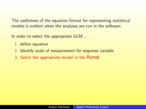
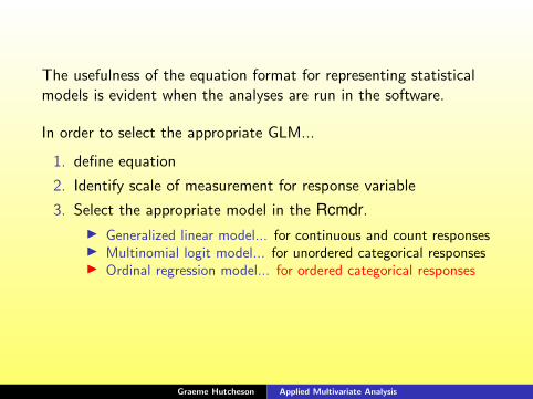
The usefulness of the equation format for representing statisticalmodels is evident when the analyses are run in the software.
In order to select the appropriate GLM...
1. define equation
2. Identify scale of measurement for response variable
3. Select the appropriate model in the Rcmdr.
I Generalized linear model... for continuous and count responsesI Multinomial logit model... for unordered categorical responsesI Ordinal regression model... for ordered categorical responses
Graeme Hutcheson Applied Multivariate Analysis
The usefulness of the equation format for representing statisticalmodels is evident when the analyses are run in the software.
In order to select the appropriate GLM...
1. define equation
2. Identify scale of measurement for response variable
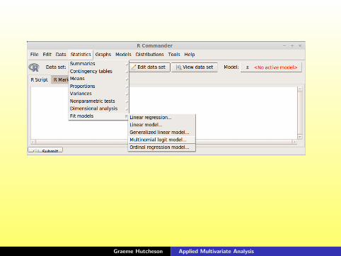
3. Select the appropriate model in the Rcmdr.
I Generalized linear model... for continuous and count responsesI Multinomial logit model... for unordered categorical responsesI Ordinal regression model... for ordered categorical responses
Graeme Hutcheson Applied Multivariate Analysis

The usefulness of the equation format for representing statisticalmodels is evident when the analyses are run in the software.
In order to select the appropriate GLM...
1. define equation
2. Identify scale of measurement for response variable
3. Select the appropriate model in the Rcmdr.I Generalized linear model... for continuous and count responses
I Multinomial logit model... for unordered categorical responsesI Ordinal regression model... for ordered categorical responses
Graeme Hutcheson Applied Multivariate Analysis

The usefulness of the equation format for representing statisticalmodels is evident when the analyses are run in the software.
In order to select the appropriate GLM...
1. define equation
2. Identify scale of measurement for response variable
3. Select the appropriate model in the Rcmdr.I Generalized linear model... for continuous and count responsesI Multinomial logit model... for unordered categorical responses
I Ordinal regression model... for ordered categorical responses
Graeme Hutcheson Applied Multivariate Analysis
The usefulness of the equation format for representing statisticalmodels is evident when the analyses are run in the software.
In order to select the appropriate GLM...
1. define equation
2. Identify scale of measurement for response variable
3. Select the appropriate model in the Rcmdr.I Generalized linear model... for continuous and count responsesI Multinomial logit model... for unordered categorical responsesI Ordinal regression model... for ordered categorical responses
Graeme Hutcheson Applied Multivariate Analysis
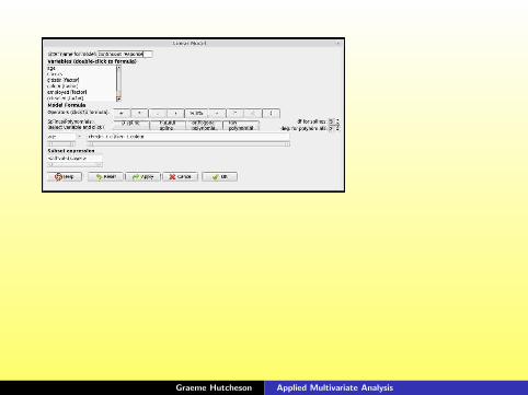
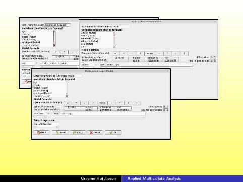
Then enter the equation...
Graeme Hutcheson Applied Multivariate Analysis

Then enter the equation...
Graeme Hutcheson Applied Multivariate Analysis
Graeme Hutcheson Applied Multivariate Analysis

Graeme Hutcheson Applied Multivariate Analysis
Graeme Hutcheson Applied Multivariate Analysis

Graeme Hutcheson Applied Multivariate Analysis

Exercises...
Graeme Hutcheson Applied Multivariate Analysis
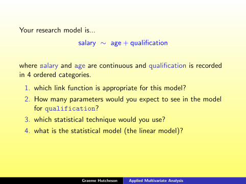
Your research model is...
salary ∼ age + qualification
where salary and age are continuous and qualification is recordedin 4 ordered categories.
1. which link function is appropriate for this model?
2. How many parameters would you expect to see in the modelfor qualification?
3. which statistical technique would you use?
4. what is the statistical model (the linear model)?
Graeme Hutcheson Applied Multivariate Analysis
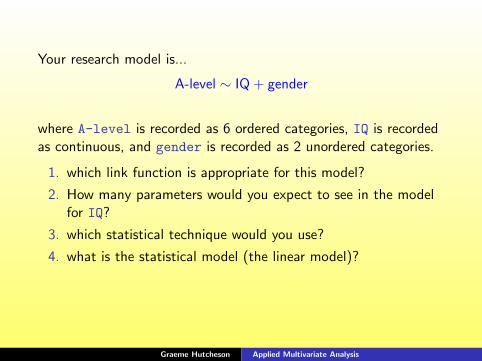
Your research model is...
A-level ∼ IQ + gender
where A-level is recorded as 6 ordered categories, IQ is recordedas continuous, and gender is recorded as 2 unordered categories.
1. which link function is appropriate for this model?
2. How many parameters would you expect to see in the modelfor IQ?
3. which statistical technique would you use?
4. what is the statistical model (the linear model)?
Graeme Hutcheson Applied Multivariate Analysis
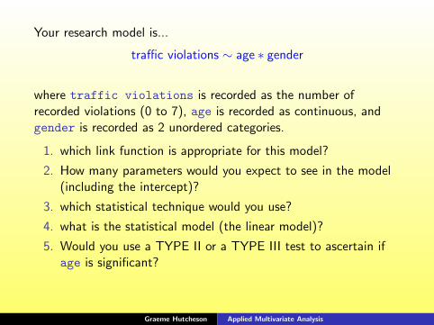
Your research model is...
traffic violations ∼ age ∗ gender
where traffic violations is recorded as the number ofrecorded violations (0 to 7), age is recorded as continuous, andgender is recorded as 2 unordered categories.
1. which link function is appropriate for this model?
2. How many parameters would you expect to see in the model(including the intercept)?
3. which statistical technique would you use?
4. what is the statistical model (the linear model)?
5. Would you use a TYPE II or a TYPE III test to ascertain ifage is significant?
Graeme Hutcheson Applied Multivariate Analysis
Your research model is...
Holiday destination ∼ age ∗ gender
where Holiday destination is recorded as 6 unorderedcategories, age is recorded as continuous, and gender is recordedas 2 unordered categories.
1. which link function is appropriate for this model?
2. which statistical technique would you use?
3. Would you use a TYPE II or a TYPE III test to ascertain ifgender is significant?
Graeme Hutcheson Applied Multivariate Analysis