applied industrial electricity
TRANSCRIPT

APPLIED INDUSTRIAL ELECTRICITY
Theory and Application
Tony R. Kuphaldt And John R. Haughery
IOWA STATE UNIVERSITY DIGITAL PRESS
AMES, IOWA

This text was originally written by Tony R. Kuphaldt and released under the Design Science License (https://www.gnu.org/licenses/dsl.html). It has since been updated by members of the All About Circuits community and editorial team. The current version was abridged by John R. Haughery.

Contents
Design Science License vii
Acknowledgements xi
1. ELECTRICAL SAFETY
1.1 Safe Practices 1
1.2 Shock Current Path 4
1.3 Just how much voltage is dangerous? 11
1.4 Zero Energy State: Securing Harmful Energy 20
1.5 Safe Meter Usage 25
1.6 Safe Circuit Design 36
1.7 Fuses 42
1
2. BASIC CONCEPTS AND RELATIONSHIPS
2.1 Static Electricity 52
2.2 Conductors, Insulators, and Electron Flow 58
2.3 What Are Electric Circuits? 63
2.4 Voltage and Current 65
2.5 Resistance 77
2.6 Resistors 83
2.7 Voltage and Current in a Practical Circuit 94
2.8 Ohm’s Law – How Voltage, Current, and Resistance Relate 95
2.9 Calculating Electric Power 103
2.9 Circuit Wiring 107
52
3. CIRCUIT TOPOLOGY AND LAWS
3.1 Simple Series Circuits 113
3.2 Using Ohm’s Law in Series Circuits 114
3.3 Simple Parallel Circuits 123
3.4 Power Calculations 128
3.5 Correct use of Ohm’s Law 130
3.6 Kirchhoff’s Voltage Law (KVL) 132
3.7 Kirchhoff’s Current Law (KCL) 145
113

4. ALTERNATING CURRENT
4.1 What is Alternating Current (AC)? 150
4.2 Measurements of AC Magnitude 156
4.3 Single-phase Power Systems 164
4.4 AC phase 173
4.5 Three-phase Power Systems 176
4.6 Phase Rotation 183
4.7 Three-phase Y and Delta Configurations 187
150
5. MOTOR CHARACTERISTICS
5.1 Introduction 197
5.2 Tesla Polyphase Induction Motors 198
5.3 Single-phase Induction Motors 216
197
6. REACTIVE POWER
6.1 AC Resistor Circuits 222
6.2 AC Inductor Circuits 223
6.3 Series Resistor Inductor Circuit 230
6.4 Parallel Resistor-Inductor Circuits 234
6.5 Inductor Quirks 238
6.6 AC Capacitor Circuits 241
6.7 Parallel Resistor-Capacitor Circuits 247
6.8 Review of R, X, and Z 250
6.9 Parallel R, L, and C 252
6.10 R, L and C Summary 255
222
7. POWER FACTOR CORRECTION
7.1 Power in Resistive and Reactive AC circuits 256
7.2 True, Reactive, and Apparent Power 262
7.3 Calculating Power Factor 269
7.4 Practical Power Factor Correction 274
256

8. TRANSFORMERS
8.1 Step-up and Step-down Transformers 282
8.2 Electrical Isolation 287
8.3 Phasing 288
8.4 Winding Configurations 293
8.5 Three-phase Transformer Circuits 300
8.6 Practical Considerations – Transformers 307
282
9. INDUSTRIAL CONTROLS
9.1 Switch Types 323
9.2 Switch Contact Design 331
9.3 Contact “Normal” State and Make/Break Sequence 336
9.4 Relay Construction 342
9.5 Time-delay Relays 345
9.6 “Ladder” Diagrams 352
9.7 Digital Logic Functions 357
9.8 Permissive and Interlock Circuits 363
323
10. MOTOR CIRCUITS AND CONTROL
10.1 Motor Control Circuits 366
10.2 Contactors 370
366
11. CONDUCTORS
11.1 Introduction to Conductance and Conductors 375
11.2 Conductor Size 377
11.3 Conductor Ampacity 386
11.4 Specific Resistance 390
11.5 Temperature Coefficient of Resistance 397
11.6 Insulator Breakdown Voltage 401
375
APPENDIX A: Right Triangle Trigonometry
Trigonometric Identities 403
The Pythagorean Theorem 404
403

APPENDIX B: Complex Number Review
Introduction to Complex Numbers 405
Vectors and AC Waveforms 409
Simple Vector Addition 412
Complex Vector Addition 416
Polar Form and Rectangular Form Notation for Complex Numbers 418
Complex Number Arithmetic 426
405
APPENDIX C: Circuit Schematic Symbols
Wires and Connections 430
Power Sources 431
Resistors Types 431
Capacitor Types 432
Inductors 432
Mutual Inductors 432
Switches, Hand Actuated 434
Switches, Process Actuated 434
Switches, Electrically Actuated (Relays) 435
Connectors 436
430
APPENDIX D: Troubleshooting - Theory And Practice
Questions to Ask Before Proceeding 438
General Troubleshooting Tips 438
Specific Troubleshooting Techniques 440
Likely Failures in Proven Systems 444
Likely Failures in Unproven Systems 446
438
Design Science License
Note that this license is not endorsed by the Free Software Foundation. It is available here as a convenience to readers of the license list.
DESIGN SCIENCE LICENSE
TERMS AND CONDITIONS FOR COPYING, DISTRIBUTION AND MODIFICATION
Copyright © 1999-2001 Michael Stutz <[email protected]> Verbatim copying of this document is permitted, in any medium.
0. PREAMBLE.
Copyright law gives certain exclusive rights to the author of a work, including the rights to copy, modify and distribute the work (the “reproductive,” “adaptative,” and “distribution” rights).
The idea of “copyleft” is to willfully revoke the exclusivity of those rights under certain terms and conditions, so that anyone can copy and distribute the work or properly attributed derivative works, while all copies remain under the same terms and conditions as the original.
The intent of this license is to be a general “copyleft” that can be applied to any kind of work that has protection under copyright. This license states those certain conditions under which a work published under its terms may be copied, distributed, and modified.
Whereas “design science” is a strategy for the development of artifacts as a way to reform the environment (not people) and subsequently improve the universal standard of living, this Design Science License was written and deployed as a strategy for promoting the progress of science and art through reform of the environment.
1. DEFINITIONS.
“License” shall mean this Design Science License. The License applies to any work which contains a notice placed by the work’s copyright holder stating that it is published under the terms of this Design Science License.
“Work” shall mean such an aforementioned work. The License also applies to the output of the Work, only if said output constitutes a “derivative work” of the licensed Work as defined by copyright law.
“Object Form” shall mean an executable or performable form of the Work, being an embodiment of the Work in some tangible medium.
“Source Data” shall mean the origin of the Object Form, being the entire, machine-readable, preferred form of the Work for copying and for human modification (usually the language, encoding or format in which composed or recorded by the Author); plus any accompanying files, scripts or other data necessary for installation, configuration or compilation of the Work.
vii

(Examples of “Source Data” include, but are not limited to, the following: if the Work is an image file composed and edited in PNG format, then the original PNG source file is the Source Data; if the Work is an MPEG 1.0 layer 3 digital audio recording made from a WAV format audio file recording of an analog source, then the original WAV file is the Source Data; if the Work was composed as an unformatted plaintext file, then that file is the Source Data; if the Work was composed in LaTeX, the LaTeX file(s) and any image files and/or custom macros necessary for compilation constitute the Source Data.)
“Author” shall mean the copyright holder(s) of the Work. The individual licensees are referred to as “you.”
2. RIGHTS AND COPYRIGHT.
The Work is copyrighted by the Author. All rights to the Work are reserved by the Author, except as specifically described below. This License describes the terms and conditions under which the Author permits you to copy, distribute and modify copies of the Work.
In addition, you may refer to the Work, talk about it, and (as dictated by “fair use”) quote from it, just as you would any copyrighted material under copyright law.
Your right to operate, perform, read or otherwise interpret and/or execute the Work is unrestricted; however, you do so at your own risk, because the Work comes WITHOUT ANY WARRANTY — see Section 7 (“NO WARRANTY”) below.
3. COPYING AND DISTRIBUTION.
Permission is granted to distribute, publish or otherwise present verbatim copies of the entire Source Data of the Work, in any medium, provided that full copyright notice and disclaimer of warranty, where applicable, is conspicuously published on all copies, and a copy of this License is distributed along with the Work.
Permission is granted to distribute, publish or otherwise present copies of the Object Form of the Work, in any medium, under the terms for distribution of Source Data above and also provided that one of the following additional conditions are met:
(a) The Source Data is included in the same distribution, distributed under the terms of this License; or
(b) A written offer is included with the distribution, valid for at least three years or for as long as the distribution is in print (whichever is longer), with a publicly-accessible address (such as a URL on the Internet) where, for a charge not greater than transportation and media costs, anyone may receive a copy of the Source Data of the Work distributed according to the section above; or
(c) A third party’s written offer for obtaining the Source Data at no cost, as described in paragraph (b) above, is included with the distribution. This option is valid only if you are a non-commercial party, and only if you received the Object Form of the Work along with such an offer.
You may copy and distribute the Work either gratis or for a fee, and if desired, you may offer warranty protection for the Work.
The aggregation of the Work with other works that are not based on the Work — such as but not limited
viii Tony R. Kuphaldt and John R. Haughery

to inclusion in a publication, broadcast, compilation, or other media — does not bring the other works in the scope of the License; nor does such aggregation void the terms of the License for the Work.
4. MODIFICATION.
Permission is granted to modify or sample from a copy of the Work, producing a derivative work, and to distribute the derivative work under the terms described in the section for distribution above, provided that the following terms are met:
(a) The new, derivative work is published under the terms of this License.
(b) The derivative work is given a new name, so that its name or title cannot be confused with the Work, or with a version of the Work, in any way.
(c) Appropriate authorship credit is given: for the differences between the Work and the new derivative work, authorship is attributed to you, while the material sampled or used from the Work remains attributed to the original Author; appropriate notice must be included with the new work indicating the nature and the dates of any modifications of the Work made by you.
5. NO RESTRICTIONS.
You may not impose any further restrictions on the Work or any of its derivative works beyond those restrictions described in this License.
6. ACCEPTANCE.
Copying, distributing or modifying the Work (including but not limited to sampling from the Work in a new work) indicates acceptance of these terms. If you do not follow the terms of this License, any rights granted to you by the License are null and void. The copying, distribution or modification of the Work outside of the terms described in this License is expressly prohibited by law.
If for any reason, conditions are imposed on you that forbid you to fulfill the conditions of this License, you may not copy, distribute or modify the Work at all.
If any part of this License is found to be in conflict with the law, that part shall be interpreted in its broadest meaning consistent with the law, and no other parts of the License shall be affected.
7. NO WARRANTY.
THE WORK IS PROVIDED “AS IS,” AND COMES WITH ABSOLUTELY NO WARRANTY, EXPRESS OR IMPLIED, TO THE EXTENT PERMITTED BY APPLICABLE LAW, INCLUDING BUT NOT LIMITED TO THE IMPLIED WARRANTIES OF MERCHANTABILITY OR FITNESS FOR A PARTICULAR PURPOSE.
8. DISCLAIMER OF LIABILITY.
IN NO EVENT SHALL THE AUTHOR OR CONTRIBUTORS BE LIABLE FOR ANY DIRECT, INDIRECT, INCIDENTAL, SPECIAL, EXEMPLARY, OR CONSEQUENTIAL DAMAGES (INCLUDING, BUT NOT LIMITED TO, PROCUREMENT OF SUBSTITUTE GOODS OR
Applied Industrial Electricity ix

SERVICES; LOSS OF USE, DATA, OR PROFITS; OR BUSINESS INTERRUPTION) HOWEVER CAUSED AND ON ANY THEORY OF LIABILITY, WHETHER IN CONTRACT, STRICT LIABILITY, OR TORT (INCLUDING NEGLIGENCE OR OTHERWISE) ARISING IN ANY WAY OUT OF THE USE OF THIS WORK, EVEN IF ADVISED OF THE POSSIBILITY OF SUCH DAMAGE.
END OF TERMS AND CONDITIONS
x Tony R. Kuphaldt and John R. Haughery

Acknowledgements
This text was adapted and formatted with the help of Oyetunji Steven Olaniba, Abbey K. Elder, Harrison W. Inefukum, and the generous financial support of Miller Open Education Mini-Grant co-sponsored by Iowa State University’s Library, Center for Excellence in Learning & Teaching (CELT), and Office of the Senior Vice President and Provost (SVPP). Cover art by Eric Van Dael.
xi

1. ELECTRICAL SAFETY
1.1 Safe Practices
The Importance of Electrical Safety
With this lesson, I hope to avoid a common mistake found in electronics textbooks of either ignoring or not covering with sufficient detail the subject of electrical safety. I assume that whoever reads this book has at least a passing interest in actually working with electricity, and as such the topic of safety is of paramount importance.
Another benefit of including a detailed lesson on electrical safety is the practical context it sets for basic concepts of voltage, current, resistance, and circuit design. The more relevant a technical topic can be made, the more likely a student will be to pay attention and comprehend. And what could be more relevant than application to your own personal safety? Also, with electrical power being such an everyday presence in modern life, almost anyone can relate to the illustrations given in such a lesson. Have you ever wondered why birds don’t get shocked while resting on power lines? Read on and find out!
Physiological Effects of Electricity
Most of us have experienced some form of electric “shock,” where electricity causes our body to experience pain or trauma. If we are fortunate, the extent of that experience is limited to tingles or jolts of pain from static electricity buildup discharging through our bodies. When we are working around electric circuits capable of delivering high power to loads, electric shock becomes a much more serious issue, and pain is the least significant result of shock.
As electric current is conducted through a material, any opposition to the current (resistance) results in a dissipation of energy, usually in the form of heat. This is the most basic and easy-to-understand effect of electricity on living tissue: current makes it heat up. If the amount of heat generated is sufficient, the tissue may be burnt. The effect is physiological, the same as damage caused by an open flame or other high-temperature source of heat, except that electricity has the ability to burn tissue well beneath the skin of a victim, even burning internal organs.
How Electric Current Affects the Nervous System
Another effect of electric current on the body, perhaps the most significant in terms of hazard, regards the nervous system. By the “nervous system”, I mean the network of special cells in the body called nerve cells or neurons which process and conduct the multitude of signals responsible for the regulation
1

of many body functions. The brain, spinal cord, and sensory/motor organs in the body function together to allow it to sense, move, respond, think, and remember.
Nerve cells communicate to each other by acting as “transducers”, creating electrical signals (very small voltages and currents) in response to the input of certain chemical compounds called neurotransmitters, and releasing these neurotransmitters when stimulated by electrical signals. If an electric current of sufficient magnitude is conducted through a living creature (human or otherwise), its effect will be to override the tiny electrical impulses normally generated by the neurons, overloading the nervous system and preventing both reflex and volitional signals from being able to actuate muscles. Muscles triggered by an external (shock) current will involuntarily contract, and there’s nothing the victim can do about it.
This problem is especially dangerous if the victim contacts an energized conductor with his or her hands. The forearm muscles responsible for bending fingers tend to be better developed than those muscles responsible for extending fingers, and so if both sets of muscles try to contract because of an electric current conducted through the person’s arm, the “bending” muscles will win, clenching the fingers into a fist. If the conductor delivering current to the victim faces the palm of his or her hand, this clenching action will force the hand to grasp the wire firmly, thus worsening the situation by securing excellent contact with the wire. The victim will be completely unable to let go of the wire.
Medically, this condition of involuntary muscle contraction is called tetanus. Electricians familiar with this effect of electric shock often refer to an immobilized victim of electric shock as being “froze on the circuit”. Shock-induced tetanus can only be interrupted by stopping the current through the victim.
Even when the current is stopped, the victim may not regain voluntary control over their muscles for a while, as the neurotransmitter chemistry has been thrown into disarray. This principle has been applied in “stun gun” devices such as Tasers, which on the principle of momentarily shocking a victim with a high-voltage pulse delivered between two electrodes. A well-placed shock has the effect of temporarily (a few minutes) immobilizing the victim.
Electric current is able to affect more than just skeletal muscles in a shock victim, however. The diaphragm muscle controlling the lungs, and the heart—which is a muscle in itself—can also be “frozen” in a state of tetanus by electric current. Even currents too low to induce tetanus are often able to scramble nerve cell signals enough that the heart cannot beat properly, sending the heart into a condition known as fibrillation. A fibrillating heart flutters rather than beat and is ineffective at pumping blood to vital organs in the body. In any case, death from asphyxiation and/or cardiac arrest will surely result from a strong enough electric current through the body. Ironically, medical personnel use a strong jolt of electric current applied across the chest of a victim to “jump-start” a fibrillating heart into a normal beating pattern.
That last detail leads us into another hazard of electric shock, this one peculiar to public power systems. Though our initial study of electric circuits will focus almost exclusively on DC (Direct Current, or electricity that moves in a continuous direction in a circuit), modern power systems utilize alternating current or AC. The technical reasons for this preference of AC over DC in power systems are irrelevant to this discussion, but the special hazards of each kind of electrical power are very important to the topic of safety.
How AC affects the body depends largely on frequency. Low-frequency (50- to 60-Hz) AC is used in US (60 Hz) and European (50 Hz) households; it can be more dangerous than high-frequency AC and is
Applied Industrial Electricity 2

3 to 5 times more dangerous than DC of the same voltage and amperage. Low-frequency AC produces extended muscle contraction (tetany), which may freeze the hand to the current’s source, prolonging exposure. DC is most likely to cause a single convulsive contraction, which often forces the victim away from the current source.
AC’s alternating nature has a greater tendency to throw the heart’s pacemaker neurons into a condition of fibrillation, whereas DC tends to just make the heart standstill. Once the shock current is halted, a “frozen” heart has a better chance of regaining a normal beat pattern than a fibrillating heart. This is why “defibrillating” equipment used by emergency medics works: the jolt of current supplied by the defibrillator unit is DC, which halts fibrillation and gives the heart a chance to recover.
In either case, electric currents high enough to cause involuntary muscle action are dangerous and are to be avoided at all costs. In the next section, we’ll take a look at how such currents typically enter and exit the body, and examine precautions against such occurrences.
Review
• Electric current is capable of producing deep and severe burns in the body due to
power dissipation across the body’s electrical resistance.
• Tetanus is the condition where muscles involuntarily contract due to the passage of
external electric current through the body. When involuntary contraction of muscles
controlling the fingers causes a victim to be unable to let go of an energized
conductor, the victim is said to be “froze on the circuit.”
• Diaphragm (lung) and heart muscles are similarly affected by electric current. Even
currents too small to induce tetanus can be strong enough to interfere with the
heart’s pacemaker neurons, causing the heart to flutter instead of strongly beat.
• Direct current (DC) is more likely to cause muscle tetanus than alternating current
(AC), making DC more likely to “freeze” a victim in a shock scenario. However,
AC is more likely to cause a victim’s heart to fibrillate, which is a more dangerous
condition for the victim after the shocking current has been halted.
3 Tony R. Kuphaldt and John R. Haughery

1.2 Shock Current Path
Electricity requires a complete path (circuit) to continuously flow. This is why the shock received from static electricity is only a momentary jolt: the flow of current is necessarily brief when static charges are equalized between two objects. Shocks of self-limited duration like this are rarely hazardous.
Without two contact points on the body for current to enter and exit, respectively, there is no hazard of shock. This is why birds can safely rest on high-voltage power lines without getting shocked: they make contact with the circuit at only one point.
Figure 1.1
In order for current to flow through a conductor, there must be a voltage present to motivate it. Voltage, as you should recall, is always relative between two points. There is no such thing as voltage “on” or “at” a single point in the circuit, and so the bird contacting a single point in the above circuit has no voltage applied across its body to establish a current through it. Yes, even though they rest on two feet, both feet are touching the same wire, making them electrically common. Electrically speaking, both of the bird’s feet touch the same point, hence there is no voltage between them to motivate current through the bird’s body.
This might lead one to believe that it’s impossible to be shocked by electricity by only touching a single wire. Like the birds, if we’re sure to touch only one wire at a time, we’ll be safe, right? Unfortunately, this is not correct. Unlike birds, people are usually standing on the ground when they contact a “live” wire. Many times, one side of a power system will be intentionally connected to earth ground, and so the person touching a single wire is actually making contact between two points in the circuit (the wire and earth ground):
Applied Industrial Electricity 4

Figure 1.2
The ground symbol is a set of three horizontal bars of decreasing width located at the lower-left of the circuit shown, and also at the foot of the person being shocked. In real life, the power system ground consists of some kind of metallic conductor buried deep in the ground for making maximum contact with the earth. That conductor is electrically connected to an appropriate connection point on the circuit with thick wire. The victim’s ground connection is through their feet, which are touching the earth.
A few questions usually arise at this point in the mind of the student:
• If the presence of a ground point in the circuit provides an easy point of contact for someone to get shocked, why have it in the circuit at all? Wouldn’t a ground-less circuit be safer?
• The person getting shocked probably isn’t bare-footed. If rubber and fabric are insulating materials, then why aren’t their shoes protecting them by preventing a circuit from forming?
• How good of a conductor can dirt be? If you can get shocked by the current through the earth, why not use the earth as a conductor in our power circuits?
In answer to the first question, the presence of an intentional “grounding” point in an electric circuit is intended to ensure that one side of it is safe to come in contact with. Note that if our victim in the above diagram were to touch the bottom side of the resistor, nothing would happen even though their feet would still be contacting ground:
5 Tony R. Kuphaldt and John R. Haughery

Figure 1.3
Because the bottom side of the circuit is firmly connected to ground through the grounding point on the lower-left of the circuit, the lower conductor of the circuit is made electrically common with earth ground. Since there can be no voltage between electrically common points, there will be no voltage applied across the person contacting the lower wire, and they will not receive a shock. For the same reason, the wire connecting the circuit to the grounding rod/plates is usually left bare (no insulation), so that any metal object it brushes up against will similarly be electrically common with the earth.
Circuit grounding ensures that at least one point in the circuit will be safe to touch. But what about leaving a circuit completely ungrounded? Wouldn’t that make any person touching just a single wire as safe as the bird sitting on just one? Ideally, yes. Practically, no. Observe what happens with no ground at all:
Figure 1.4
Applied Industrial Electricity 6

Despite the fact that the person’s feet are still contacting the ground, any single point in the circuit should be safe to touch. Since there is no complete path (circuit) formed through the person’s body from the bottom side of the voltage source to the top, there is no way for a current to be established through the person. However, this could all change with an accidental ground, such as a tree branch touching a power line and providing the connection to earth ground. Such an accidental connection between a power system conductor and the earth (ground) is called a ground fault.
Figure 1.5
Ground Faults
Ground faults may be caused by many things, including dirt buildup on power line insulators (creating a dirty-water path for current from the conductor to the pole, and to the ground, when it rains), groundwater infiltration in buried power line conductors, and birds landing on power lines, bridging the line to the pole with their wings. Given the many causes of ground faults, they tend to be unpredictable. In the case of trees, no one can guarantee which wire their branches might touch. If a tree were to brush up against the top wire in the circuit, it would make the top wire safe to touch and the bottom one dangerous—just the opposite of the previous scenario where the tree contacts the bottom wire:
7 Tony R. Kuphaldt and John R. Haughery

Figure 1.6
With a tree branch contacting the top wire, that wire becomes the grounded conductor in the circuit, electrically common with earth ground. Therefore, there is no voltage between that wire and ground, but full (high) voltage between the bottom wire and ground. As mentioned previously, tree branches are only one potential source of ground faults in a power system. Consider an ungrounded power system with no trees in contact, but this time with two people touching single wires:
Applied Industrial Electricity 8

Figure 1.7
With each person standing on the ground, contacting different points in the circuit, a path for shock current is made through one person, through the earth, and through the other person. Even though each person thinks they’re safe in only touching a single point in the circuit, their combined actions create a deadly scenario. In effect, one person acts as the ground fault which makes it unsafe for the other person. This is exactly why ungrounded power systems are dangerous: the voltage between any point in the circuit and ground (earth) is unpredictable because a ground fault could appear at any point in the circuit at any time. The only character guaranteed to be safe in these scenarios is the bird, who has no connection to earth ground at all! By firmly connecting a designated point in the circuit to earth ground (“grounding” the circuit), at least safety can be assured at that one point. This is more assurance of safety than having no ground connection at all.
In answer to the second question, rubber-soled shoes do indeed provide some electrical insulation to help protect someone from conducting shock current through their feet. However, most common shoe designs are not intended to be electrically “safe,” their soles being too thin and not of the right substance. Also, any moisture, dirt, or conductive salts from body sweat on the surface of or permeated through the soles of shoes will compromise what little insulating value the shoe had to begin with. There are shoes specifically made for dangerous electrical work, as well as thick rubber mats made to stand on while working on live circuits, but these special pieces of gear must be in the absolutely clean, dry condition in order to be effective. Suffice it to say, normal footwear is not enough to guarantee protection against electric shock from a power system.
Research conducted on contact resistance between parts of the human body and points of contact (such as the ground) shows a wide range of figures (see the end of the chapter for information on the source of this data):
• Hand or foot contact, insulated with rubber: 20 MΩ typical.
9 Tony R. Kuphaldt and John R. Haughery

• Foot contact through leather shoe sole (dry): 100 kΩ to 500 kΩ
• Foot contact through leather shoe sole (wet): 5 kΩ to 20 kΩ
As you can see, not only is rubber a far better insulating material than leather, but the presence of water in a porous substance such as leather greatly reduces electrical resistance.
In answer to the third question, dirt is not a very good conductor (at least not when it’s dry!). It is too poor of a conductor to support continuous current for powering a load. However, as we will see in the next section, it takes very little current to injure or kill a human being, so even the poor conductivity of dirt is enough to provide a path for deadly current when there is sufficient voltage available, as there usually is in power systems.
Some ground surfaces are better insulators than others. Asphalt, for instance, being oil-based, has a much greater resistance than most forms of dirt or rock. Concrete, on the other hand, tends to have fairly low resistance due to its intrinsic water and electrolyte (conductive chemical) content.
Review
• Electric shock can only occur when contact is made between two points of a circuit;
when voltage is applied across a victim’s body.
• Power circuits usually have a designated point that is “grounded:” firmly connected
to metal rods or plates buried in the dirt to ensure that one side of the circuit is
always at ground potential (zero voltage between that point and earth ground).
• A ground fault is an accidental connection between a circuit conductor and the earth
(ground).
• Special, insulated shoes and mats are made to protect persons from shock via
ground conduction, but even these pieces of gear must be in clean, dry condition to
be effective. Normal footwear is not good enough to provide protection from shock
by insulating its wearer from the earth.
• Though dirt is a poor conductor, it can conduct enough current to injure or kill a
human being.
Applied Industrial Electricity 10

1.3 Just how much voltage is dangerous?
A common phrase heard in reference to electrical safety goes something like this: “It’s not the voltage that kills, it’s current!” While there is an element of truth to this, there’s more to understand about shock hazard than this simple adage. If the voltage presented no danger, no one would ever print and display signs saying: DANGER—HIGH VOLTAGE!
The principle that “current kills” is essentially correct. It is an electric current that burns tissue, freezes muscles, and fibrillates hearts. However, electric current doesn’t just occur on its own: there must be voltage available to motivate the current to flow through a victim. A person’s body also presents resistance to the current, which must be taken into account.
Taking Ohm’s Law for voltage, current, and resistance, and expressing it in terms of current for a given voltage and resistance, we have this equation:
The amount of current through a body is equal to the amount of voltage applied between two points on that body, divided by the electrical resistance offered by the body between those two points. Obviously, the more voltage available to cause the current to flow, the easier it will flow through any given amount of resistance. Hence, the danger of high voltage that can generate enough current to cause injury or death. Conversely, if a body presents higher resistance, less current will flow for any given amount of voltage. Just how much voltage is dangerous depends on how much total resistance is in the circuit to oppose the flow of electric current.
Body resistance is not a fixed quantity. It varies from person to person and from time to time. There’s even a body fat measurement technique based on a measurement of electrical resistance between a person’s toes and fingers. Differing percentages of body fat provide different resistances: one variable affecting electrical resistance in the human body. In order for the technique to work accurately, the person must regulate their fluid intake for several hours prior to the test, indicating that body hydration is another factor impacting the body’s electrical resistance.
Body resistance also varies depending on how contact is made with the skin: from hand-to-hand, hand-to-foot, foot-to-foot, hand-to-elbow, etc. Sweat, being rich in salt and minerals, is an excellent conductor of electricity for being a liquid. So is blood with its similarly high content of conductive chemicals. Thus, contact with a wire made by a sweaty hand or open wound will offer much less resistance to current than contact made by clean, dry skin.
11 Tony R. Kuphaldt and John R. Haughery

Measuring electrical resistance with a sensitive meter, I approximately measure 1 million ohms of resistance (1 MΩ) on my hands holding on to the meter’s metal probes between my fingers. The meter indicates less resistance when I squeezed the probes tightly and more resistance when I hold them loosely. Sitting here at my computer, typing these words, my hands are clean and dry. If I were working in some hot, dirty, industrial environment, the resistance between my hands would likely be much less, presenting less opposition to deadly current, and a greater threat of electrical shock.
How Much Electric Current is Harmful?
The answer to that question also depends on several factors. Individual body chemistry has a significant impact on how electric current affects an individual. Some people are highly sensitive to current, experiencing involuntary muscle contraction with shocks from static electricity. Others can draw large sparks from discharging static electricity and hardly feel it, much less experience a muscle spasm. Despite these differences, approximate guidelines have been developed through tests that indicate very little current being necessary to manifest harmful effects (again, see the end of the chapter for information on the source of this data). All current figures given in milliamps (a milliamp is equal to 1/1000 of an amp):
Applied Industrial Electricity 12

BODILY EFFECT MEN/WOMEN DIRECT CURRENT (DC) 60Hz 100KHz
Slight sensation felt at hand(s) Men 1.0 mA 0.4 mA 7mA
Women 0.6 mA 0.3 mA 5 mA
Threshold of Pain Men 5.2 mA 1.1 mA 12 mA
Women 3.5 mA 0.7 mA 8 mA
Painful, but voluntary muscles control maintained Men 62 mA 9 mA 55 mA
Women 41 mA 6 mA 37 mA
Painful, unable to let go of wires Men 76 mA 16 mA 75 mA
Women 60 mA 15 mA 63 mA
Severe pain, difficulty breathing Men 90 mA 23 mA 94 mA
Women 60 mA 15 mA 63 mA
Possible heart fibrillation after 3 seconds Men and Women 500 mA 100 mA
“Hz” stands for the unit Hertz. It is the measure of how rapidly alternating current alternates, otherwise known as frequency. So, the column of figures labeled “60 Hz AC” refers to a current that alternates at a frequency of 60 cycles (1 cycle = period of time where current flows in one direction, then the other direction) per second. The last column, labeled “10 kHz AC,” refers to alternating current that completes ten thousand (10,000) back-and-forth cycles each and every second.
Keep in mind that these figures are only approximate, as individuals with different body chemistry may react differently. It has been suggested that an across-the-chest current of only 17 milliamps AC is enough to induce fibrillation in a human subject under certain conditions. Most of our data regarding induced fibrillation come from animal testing. Obviously, it is not practical to perform tests of induced ventricular fibrillation on human subjects, so the available data is sketchy. Oh, and in case you’re wondering, I have no idea why women tend to be more susceptible to electric currents than men! Suppose I were to place my hands across the terminals of an AC voltage source at 60 Hz (60 cycles per second). How much voltage would be necessary on this clean, dry-skin condition to produce a current of 20 milliamps (enough to cause me to become unable to let go of the voltage source)? We can use Ohm’s Law to determine this:
13 Tony R. Kuphaldt and John R. Haughery
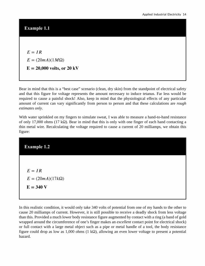
Example 1.1
Bear in mind that this is a “best case” scenario (clean, dry skin) from the standpoint of electrical safety and that this figure for voltage represents the amount necessary to induce tetanus. Far less would be required to cause a painful shock! Also, keep in mind that the physiological effects of any particular amount of current can vary significantly from person to person and that these calculations are rough estimates only.
With water sprinkled on my fingers to simulate sweat, I was able to measure a hand-to-hand resistance of only 17,000 ohms (17 kΩ). Bear in mind that this is only with one finger of each hand contacting a thin metal wire. Recalculating the voltage required to cause a current of 20 milliamps, we obtain this figure:
Example 1.2
In this realistic condition, it would only take 340 volts of potential from one of my hands to the other to cause 20 milliamps of current. However, it is still possible to receive a deadly shock from less voltage than this. Provided a much lower body resistance figure augmented by contact with a ring (a band of gold wrapped around the circumference of one’s finger makes an excellent contact point for electrical shock) or full contact with a large metal object such as a pipe or metal handle of a tool, the body resistance figure could drop as low as 1,000 ohms (1 kΩ), allowing an even lower voltage to present a potential hazard.
Applied Industrial Electricity 14

Example 1.3
Notice that in this condition, 20 volts is enough to produce a current of 20 milliamps through a person; enough to induce tetanus. Remember, it has been suggested a current of only 17 milliamps may induce ventricular (heart) fibrillation. With a hand-to-hand resistance of 1000 Ω, it would only take 17 volts to create this dangerous condition.
Example 1.4
Seventeen volts is not very much as far as electrical systems are concerned. Granted, this is a “worst-case” scenario with 60 Hz AC voltage and excellent bodily conductivity, but it does stand to show how little voltage may present a serious threat under certain conditions.
The conditions necessary to produce 1,000 Ω of body resistance don’t have to be as extreme as what was presented (sweaty skin with contact made on a gold ring). Body resistance may decrease with the application of voltage (especially if tetanus causes the victim to maintain a tighter grip on a conductor) so that with constant voltage a shock may increase in severity after initial contact. What begins as a mild shock—just enough to “freeze” a victim so they can’t let go—may escalate into something severe enough to kill them as their body resistance decreases and current correspondingly increases.
Research has provided an approximate set of figures for electrical resistance of human contact points under different conditions:
15 Tony R. Kuphaldt and John R. Haughery
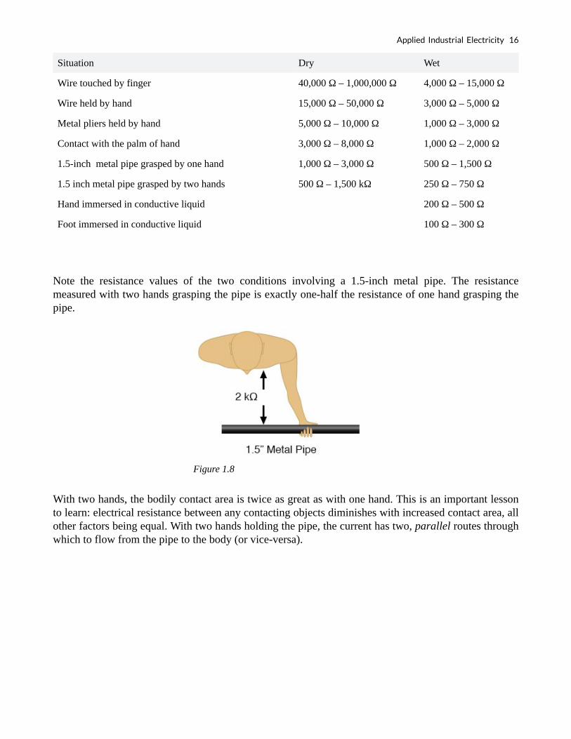
Situation Dry Wet
Wire touched by finger 40,000 Ω – 1,000,000 Ω 4,000 Ω – 15,000 Ω
Wire held by hand 15,000 Ω – 50,000 Ω 3,000 Ω – 5,000 Ω
Metal pliers held by hand 5,000 Ω – 10,000 Ω 1,000 Ω – 3,000 Ω
Contact with the palm of hand 3,000 Ω – 8,000 Ω 1,000 Ω – 2,000 Ω
1.5-inch metal pipe grasped by one hand 1,000 Ω – 3,000 Ω 500 Ω – 1,500 Ω
1.5 inch metal pipe grasped by two hands 500 Ω – 1,500 kΩ 250 Ω – 750 Ω
Hand immersed in conductive liquid 200 Ω – 500 Ω
Foot immersed in conductive liquid 100 Ω – 300 Ω
Note the resistance values of the two conditions involving a 1.5-inch metal pipe. The resistance measured with two hands grasping the pipe is exactly one-half the resistance of one hand grasping the pipe.
Figure 1.8
With two hands, the bodily contact area is twice as great as with one hand. This is an important lesson to learn: electrical resistance between any contacting objects diminishes with increased contact area, all other factors being equal. With two hands holding the pipe, the current has two, parallel routes through which to flow from the pipe to the body (or vice-versa).
Applied Industrial Electricity 16

Figure 1.9
As we will see in a later chapter, parallel circuit pathways always result in less overall resistance than any single pathway considered alone.
In industry, 30 volts is generally considered to be a conservative threshold value for dangerous voltage. The cautious person should regard any voltage above 30 volts as threatening, not relying on normal body resistance for protection against shock. That being said, it is still an excellent idea to keep one’s hands clean and dry and remove all metal jewelry when working around electricity. Even around lower voltages, metal jewelry can present a hazard by conducting enough current to burn the skin if brought into contact between two points in a circuit. Metal rings, especially, have been the cause of more than a few burnt fingers by bridging between points in a low-voltage, high-current circuit.
Also, voltages lower than 30 can be dangerous if they are enough to induce an unpleasant sensation, which may cause you to jerk and accidentally come into contact across a higher voltage or some other hazard. I recall once working on an automobile on a hot summer day. I was wearing shorts, my bare leg contacting the chrome bumper of the vehicle as I tighten battery connections. When I touched my metal wrench to the positive (ungrounded) side of the 12-volt battery, I could feel a tingling sensation at the point where my leg was touching the bumper. The combination of firm contact with metal and my sweaty skin made it possible to feel a shock with only 12 volts of electrical potential.
Thankfully, nothing bad happened but had the engine been running and the shock felt at my hand instead of my leg, I might have reflexively jerked my arm into the path of the rotating fan, or dropped the metal wrench across the battery terminals (producing large amounts of current through the wrench with lots of accompanying sparks). This illustrates another important lesson regarding electrical safety; that electric current itself may be an indirect cause of injury by causing you to jump or spasm parts of your body into harm’s way.
The path current takes through the human body makes a difference as to how harmful it is. Current will affect whatever muscles are in its path, and since the heart and lung (diaphragm) muscles are probably the most critical to one’s survival, shock paths traversing the chest are the most dangerous. This makes the hand-to-hand shock current path a very likely mode of injury and fatality.
17 Tony R. Kuphaldt and John R. Haughery

To guard against such an occurrence, it is advisable to only use one hand to work on live circuits of hazardous voltage, keeping the other hand tucked into a pocket so as to not accidentally touch anything. Of course, it is always safer to work on a circuit when it is unpowered, but this is not always practical or possible. For one-handed work, the right hand is generally preferred over the left for two reasons: most people are right-handed (thus granting additional coordination when working), and the heart is usually situated to the left of center in the chest cavity.
For those who are left-handed, this advice may not be the best. If such a person is sufficiently uncoordinated with their right hand, they may be placing themselves in greater danger by using the hand they’re least comfortable with, even if shock current through that hand might present more of a hazard to their heart. The relative hazard between shock through one hand or the other is probably less than the hazard of working with less than optimal coordination, so the choice of which hand to work with is best left to the individual.
The best protection against shock from a live circuit is resistance, and resistance can be added to the body through the use of insulated tools, gloves, boots, and other gear. Current in a circuit is a function of available voltage divided by the total resistance in the path of the flow. As we will investigate in greater detail later in this book, resistances have an additive effect when they’re stacked up so that there’s only one path for current to flow:
Figure 1.10
Example 1.5
Person in direct contact with voltage source: current limited only by body resistance.
Applied Industrial Electricity 18

Now we’ll see an equivalent circuit for a person wearing insulated gloves and boots:
Figure 1.11
Example 1.6
Person wearing insulating gloves and boots;
Current now limited by circuit resistance:
Because electric current must pass through the boot and the body and the glove to complete its circuit back to the battery, the combined total (sum) of these resistances opposes the flow of current to a greater degree than any of the resistances considered individually.
Safety is one of the reasons electrical wires are usually covered with plastic or rubber insulation: to vastly increase the amount of resistance between the conductor and whoever or whatever might contact it. Unfortunately, it would be prohibitively expensive to enclose power line conductors’ insufficient insulation to provide safety in case of accidental contact. So safety is maintained by keeping those lines far enough out of reach so that no one can accidentally touch them.
If at all possible, shut off the power to a circuit before performing any work on it. You must secure all sources of harmful energy before a system may be considered safe to work on. In industry, securing
19 Tony R. Kuphaldt and John R. Haughery

a circuit, device, or system in this condition is commonly known as placing it in a Zero Energy State. The focus of this lesson is, of course, electrical safety. However, many of these principles apply to non-electrical systems as well.
Review
• Harm to the body is a function of the amount of shock current. Higher voltage allows
for the production of higher, more dangerous currents. Resistance opposes current,
making high resistance a good protective measure against shock.
• Any voltage above 30 is generally considered to be capable of delivering dangerous
shock currents. Metal jewelry is definitely bad to wear when working around electric
circuits. Rings, watchbands, necklaces, bracelets, and other such adornments provide
excellent electrical contact with your body and can conduct current themselves
enough to produce skin burns, even with low voltages.
• Low voltages can still be dangerous even if they’re too low to directly cause shock
injury. They may be enough to startle the victim, causing them to jerk back and
contact something more dangerous in the near vicinity.
• When necessary to work on a “live” circuit, it is best to perform the work with one
hand so as to prevent a deadly hand-to-hand (through the chest) shock current path.
• If at all possible, shut off the power to a circuit before performing any work on it.
1.4 Zero Energy State: Securing Harmful Energy
When working on equipment, remove all sources of power before performing any work. In industry, removing these sources of power from a circuit, device, or system is commonly known as placing it in a Zero Energy State. The focus of this lesson is, of course, electrical safety. However, many of these principles apply to non-electrical systems as well.
Securing something in a Zero Energy State means ridding it of any sort of potential or stored energy, including but not limited to:
• Dangerous voltage
• Spring pressure
Applied Industrial Electricity 20

• Hydraulic (liquid) pressure
• Pneumatic (air) pressure
• Suspended weight
• Chemical energy (flammable or otherwise reactive substances)
• Nuclear energy (radioactive or fissile substances)
Voltage by its very nature is a manifestation of potential energy. In the first chapter, I even used the elevated liquid as an analogy for the potential energy of voltage, having the capacity (potential) to produce a current (flow), but not necessarily realizing that potential until a suitable path for flow has been established and resistance to flow is overcome. A pair of wires with a high voltage between them do not look or sound dangerous even though they harbor enough potential energy between them to push deadly amounts of current through your body. Even though that voltage isn’t presently doing anything, it has the potential to, and that potential must be neutralized before it is safe to physically contact those wires.
All properly designed circuits have “disconnect” switch mechanisms for securing voltage from a circuit. Sometimes these “disconnects” serve a dual purpose of automatically opening under excessive current conditions, in which case we call them “circuit breakers”. Other times, the disconnecting switches are strictly manually-operated devices with no automatic function. In either case, they are there for your protection and must be used properly. Please note that the disconnect device should be separate from the regular switch used to turn the device on and off. It is a safety switch, to be used only for securing the system in a Zero Energy State:
Figure 1.12
With the disconnect switch in the “open” position as shown (no continuity), the circuit is broken and no current will exist. There will be zero voltage across the load, and the full voltage of the source will be dropped across the open contacts of the disconnect switch. Note how there is no need for a disconnect switch in the lower conductor of the circuit. Because that side of the circuit is firmly connected to the earth (ground), it is electrically common with the earth and is best left that way. For maximum safety of personnel working on a load of this circuit, a temporary ground connection could be established on the top side of the load, to ensure that no voltage could ever be dropped across the load:
21 Tony R. Kuphaldt and John R. Haughery

Figure 1.13
With the temporary ground connection in place, both sides of the load wiring are connected to ground, securing a Zero Energy State at the load.
Since a ground connection made on both sides of the load is electrically equivalent to short-circuiting across the load with a wire, that is another way of accomplishing the same goal of maximum safety:
Figure 1.14
Either way, both sides of the load will be electrically common to the earth, allowing for no voltage (potential energy) between either side of the load and the ground people stand on. This technique of temporarily grounding conductors in a de-energized power system is very common in maintenance work performed on high voltage power distribution systems.
A further benefit of this precaution is protection against the possibility of the disconnect switch being closed (turned “on” so that circuit continuity is established) while people are still contacting the load. The temporary wire connected across the load would create a short-circuit when the disconnect switch was closed, immediately tripping any overcurrent protection devices (circuit breakers or fuses) in the circuit, which would shut the power off again. Damage may very well be sustained by the disconnect switch if this were to happen, but the workers at the load are kept safe.
Applied Industrial Electricity 22

It would be good to mention at this point that overcurrent devices are not intended to provide protection against electric shock. Rather, they exist solely to protect conductors from overheating due to excessive currents. The temporary shorting wires just described would indeed cause any overcurrent devices in the circuit to “trip” if the disconnect switch were to be closed, but realize that electric shock protection is not the intended function of those devices. Their primary function would merely be leveraged for the purpose of worker protection with the shorting wire in place.
Structured Safety Systems: Lock-out/Tag-out
Since it is obviously important to be able to secure any disconnecting devices in the open (off) position and make sure they stay that way while work is being done on the circuit, there is a need for a structured safety system to be put into place. Such a system is commonly used in industry and it is called Lock-out/Tag-out.
A lock-out/tag-out procedure works like this: all individuals working on a secured circuit have their own personal padlock or combination lock which they set on the control lever of a disconnect device prior to working on the system. Additionally, they must fill out and sign a tag which they hang from their lock describing the nature and duration of the work they intend to perform on the system. If there are multiple sources of energy to be “locked out” (multiple disconnects, both electrical and mechanical energy sources to be secured, etc.), the worker must use as many of his or her locks as necessary to secure power from the system before work begins. This way, the system is maintained in a Zero Energy State until every last lock is removed from all the disconnect and shut off devices, and that means every last worker gives consent by removing their own personal locks. If the decision is made to re-energize the system and one person’s lock(s) still remain in place after everyone present removes theirs, the tag(s) will show who that person is and what it is they’re doing.
Even with a good lock-out/tag-out safety program in place, there is still a need for diligence and common-sense precaution. This is especially true in industrial settings where a multitude of people may be working on a device or system at once. Some of those people might not know about proper lock-out/tag-out procedure, or might know about it but are too complacent to follow it. Don’t assume that everyone has followed the safety rules!
After an electrical system has been locked out and tagged with your own personal lock, you must then double-check to see if the voltage really has been secured in a zero state. One way to check is to see if the machine (or whatever it is that’s being worked on) will startup if the start switch or button is actuated. If it starts, then you know you haven’t successfully secured the electrical power from it.
Additionally, you should always check for the presence of dangerous voltage with a measuring device before actually touching any conductors in the circuit. To be safest, you should follow this procedure of checking, using, and then checking your meter:
• Check to see that your meter indicates properly on a known source of voltage.
• Use your meter to test the locked-out circuit for any dangerous voltage.
• Check your meter once more on a known source of voltage to see that it still indicates as it should.
23 Tony R. Kuphaldt and John R. Haughery

While this may seem excessive or even paranoid, it is a proven technique for preventing electrical shock. I once had a meter fail to indicate voltage when it should have while checking a circuit to see if it was “dead.” Had I not used other means to check for the presence of voltage, I might not be alive today to write this. There’s always the chance that your voltage meter will be defective just when you need it to check for a dangerous condition. Following these steps will help ensure that you’re never misled into a deadly situation by a broken meter.
Finally, the electrical worker will arrive at a point in the safety check procedure where it is deemed safe to actually touch the conductor(s). Bear in mind that after all of the precautionary steps have taken, it is still possible (although very unlikely) that a dangerous voltage may be present. One final precautionary measure to take at this point is to make momentary contact with the conductor(s) with the back of the hand before grasping it or a metal tool in contact with it. Why? If for some reason, there is still voltage present between that conductor and earth ground, finger motion from the shock reaction (clenching into a fist) will break contact with the conductor. Please note that this is absolutely the last step that any electrical worker should ever take before beginning work on a power system, and should never be used as an alternative method of checking for dangerous voltage. If you ever have reason to doubt the trustworthiness of your meter, use another meter to obtain a “second opinion
Review
• Zero Energy State: When a circuit, device, or system has been secured so that no
potential energy exists to harm someone working on it.
• Disconnect switch devices must be present in a properly designed electrical system
to allow for convenient readiness of a Zero Energy State.
• Temporary grounding or shorting wires may be connected to a load being serviced
for extra protection to personnel working on that load.
• Lock-out/Tag-out works like this: when working on a system in a Zero Energy
State, the worker places a personal padlock or combination lock on every energy
disconnect device relevant to his or her task on that system. Also, a tag is hung on
every one of those locks describing the nature and duration of the work to be done,
and who is doing it.
• Always verify that a circuit has been secured in a Zero Energy State with test
equipment after “locking it out.” Be sure to test your meter before and after checking
the circuit to verify that it is working properly.
• When the time comes to actually make contact with the conductor(s) of a supposedly
Applied Industrial Electricity 24

dead power system, do so first with the back of one hand so that if a shock should
occur, the muscle reaction will pull the fingers away from the conductor.
1.5 Safe Meter Usage
Using an electrical meter safely and efficiently is perhaps the most valuable skill an electronics technician can master, both for the sake of their own personal safety and for proficiency at their trade. It can be daunting at first to use a meter, knowing that you are connecting it to live circuits which may harbor life-threatening levels of voltage and current. This concern is not unfounded, and it is always best to proceed cautiously when using meters. Carelessness more than any other factor is what causes experienced technicians to have electrical accidents.
Multimeters
The most common piece of electrical test equipment is a meter called the multimeter. Multimeters are so named because they have the ability to measure a multiple of variables: voltage, current, resistance, and often many others, some of which cannot be explained here due to their complexity. In the hands of a trained technician, the multimeter is both an efficient work tool and a safety device. In the hands of someone ignorant and/or careless, however, the multimeter may become a source of danger when connected to a “live” circuit.
There are many different brands of multimeters, with multiple models made by each manufacturer sporting different sets of features. The multimeter shown here in the following illustrations is a “generic” design, not specific to any manufacturer, but general enough to teach the basic principles of use:
Figure 1.15
25 Tony R. Kuphaldt and John R. Haughery

You will notice that the display of this meter is of the “digital” type: showing numerical values using four digits in a manner similar to a digital clock. The rotary selector switch (now set in the Off position) has five different measurement positions it can be set in: two “V” settings, two “A” settings, and one set in the middle with a funny-looking “horseshoe” symbol on it representing “resistance.” The “horseshoe” symbol is the Greek letter “Omega” (Ω), which is the common symbol for the electrical unit of ohms.
Of the two “V” settings and two “A” settings, you will notice that each pair is divided into unique markers with either a pair of horizontal lines (one solid, one dashed) or a dashed line with a squiggly curve over it. The parallel lines represent “DC” while the squiggly curve represents “AC.” The “V” of course stands for “voltage” while the “A” stands for “amperage” (current). The meter uses different techniques, internally, to measure DC than it uses to measure AC, and so it requires the user to select which type of voltage (V) or current (A) is to be measured. Although we haven’t discussed alternating current (AC) in any technical detail, this distinction in meter settings is an important one to bear in mind.
Multimeter Sockets
There are three different sockets on the multimeter face into which we can plug our test leads. Test leads are nothing more than specially-prepared wires used to connect the meter to the circuit under test. The wires are coated in a color-coded (either black or red) flexible insulation to prevent the user’s hands from contacting the bare conductors, and the tips of the probes are sharp, stiff pieces of wire:
Figure 1.16
The black test lead always plugs into the black socket on the multimeter: the one marked “COM” for “common.” The red test leads plugs into either the red socket marked for voltage and resistance or the red socket marked for current, depending on which quantity you intend to measure with the multimeter.
Applied Industrial Electricity 26

To see how this works, let’s look at a couple of examples showing the meter in use. First, we’ll set up the meter to measure DC voltage from a battery:
Figure 1.17
Note that the two test leads are plugged into the appropriate sockets on the meter for voltage, and the selector switch has been set for DC “V”. Now, we’ll take a look at an example of using the multimeter to measure AC voltage from a household electrical power receptacle (wall socket):
Figure 1.18
The only difference in the setup of the meter is the placement of the selector switch: it is now turned to AC “V”. Since we’re still measuring voltage, the test leads will remain plugged in the same sockets. In both of these examples, it is imperative that you not let the probe tips come in contact with one another while they are both in contact with their respective points on the circuit. If this happens, a short-circuit will be formed, creating a spark and perhaps even a ball of flame if the voltage source is capable of supplying enough current! The following image illustrates the potential for hazard:
27 Tony R. Kuphaldt and John R. Haughery

Figure 1.19
This is just one of the ways that a meter can become a source of the hazard if used improperly.
Voltage measurement is perhaps the most common function a multimeter is used for. It is certainly the primary measurement taken for safety purposes (part of the lock-out/tag-out procedure), and it should be well understood by the operator of the meter. Being that voltage is always relative between two points, the meter must be firmly connected to two points in a circuit before it will provide a reliable measurement. That usually means both probes must be grasped by the user’s hands and held against the proper contact points of a voltage source or circuit while measuring.
Because a hand-to-hand shock current path is the most dangerous, holding the meter probes on two points in a high-voltage circuit in this manner is always a potential hazard. If the protective insulation on the probes is worn or cracked, it is possible for the user’s fingers to come into contact with the probe conductors during the time of the test, causing a bad shock to occur. If it is possible to use only one hand to grasp the probes, that is a safer option. Sometimes it is possible to “latch” one probe tip onto the circuit test point so that it can be let go of and the other probe set in place, using only one hand. Special probe tip accessories such as spring clips can be attached to help facilitate this.
Remember that meter test leads are part of the whole equipment package and that they should be treated with the same care and respect that the meter itself is. If you need a special accessory for your test leads, such as a spring clip or other special probe tip, consult the product catalog of the meter manufacturer or other test equipment manufacturer. Do not try to be creative and make your own test probes, as you may end up placing yourself in danger the next time you use them on a live circuit.
Also, it must be remembered that digital multimeters usually do a good job of discriminating between AC and DC measurements, as they are set for one or the other when checking for voltage or current. As we have seen earlier, both AC and DC voltages and currents can be deadly, so when using a multimeter as a safety check device you should always check for the presence of both AC and DC, even if you’re not expecting to find both! Also, when checking for the presence of hazardous voltage, you should be sure to check all pairs of points in question.
For example, suppose that you opened up an electrical wiring cabinet to find three large conductors supplying AC power to a load. The circuit breaker feeding these wires (supposedly) has been shut off,
Applied Industrial Electricity 28

locked, and tagged. You double-checked the absence of power by pressing the Start button for the load. Nothing happened, so now you move on to the third phase of your safety check: the meter test for voltage.
First, you check your meter on a known source of voltage to see that it’s working properly. Any nearby power receptacle should provide a convenient source of AC voltage for a test. You do so and find that the meter indicates as it should. Next, you need to check for voltage among these three wires in the cabinet. But voltage is measured between two points, so where do you check?
Figure 1.20
The answer is to check between all combinations of those three points. As you can see, the points are labeled “A”, “B”, and “C” in the illustration, so you would need to take your multimeter (set in the voltmeter mode) and check between points A & B, B & C, and A & C. If you find voltage between any of those pairs, the circuit is not in a Zero Energy State. But wait! Remember that a multimeter will not register DC voltage when it’s in the AC voltage mode and vice versa, so you need to check those three pairs of points in each mode for a total of six voltage checks in order to be complete!
However, even with all that checking, we still haven’t covered all possibilities yet. Remember that hazardous voltage can appear between a single wire and ground (in this case, the metal frame of the cabinet would be a good ground reference point) in a power system. So, to be perfectly safe, we not only have to check between A & B, B & C, and A & C (in both AC and DC modes), but we also have to check between A & ground, B & ground, and C & ground (in both AC and DC modes)! This makes for a grand total of twelve voltage checks for this seemingly simple scenario of only three wires. Then, of course, after we’ve completed all these checks, we need to take our multimeter and re-test it against a known source of voltage such as a power receptacle to ensure that it’s still in good working order.
29 Tony R. Kuphaldt and John R. Haughery

Using a Multimeter to Check for Resistance
Using a multimeter to check for resistance is a much simpler task. The test leads will be kept plugged in the same sockets as for the voltage checks, but the selector switch will need to be turned until it points to the “horseshoe” resistance symbol. Touching the probes across the device whose resistance is to be measured, the meter should properly display the resistance in ohms:
Figure 1.21
One very important thing to remember about measuring resistance is that it must only be done on de-energized components! When the meter is in “resistance” mode, it uses a small internal battery to generate a tiny current through the component to be measured. By sensing how difficult it is to move this current through the component, the resistance of that component can be determined and displayed. If there is an additional source of voltage in the meter-lead-component-lead-meter loop to either aid or oppose the resistance-measuring current produced by the meter, faulty readings will result. In a worse-case situation, the meter may even be damaged by the external voltage.
The “Resistance” Mode of a Multimeter
The “resistance” mode of a multimeter is very useful in determining wire continuity as well as making precise measurements of resistance. When there is a good, solid connection between the probe tips (simulated by touching them together), the meter shows almost zero Ω. If the test leads had no resistance in them, it would read exactly zero:
Applied Industrial Electricity 30

Figure 1.22
If the leads are not in contact with each other or touching opposite ends of a broken wire, the meter will indicate infinite resistance (usually by displaying dashed lines or the abbreviation “O.L.” which stands for “open-loop”):
Figure 1.23
Measuring Current with a Multimeter
By far the most hazardous and complex application of the multimeter is in the measurement of current. The reason for this is quite simple: in order for the meter to measure current, the current to be measured must be forced to go through the meter. This means that the meter must be made part of the current path of the circuit rather than just be connected off to the side somewhere as is the case when measuring voltage. In order to make the meter part of the current path of the circuit, the original circuit must be “broken” and the meter connected across the two points of the open break. To set the meter up for this, the selector switch must point to either AC or DC “A” and the red test lead must be plugged in the red socket marked “A”. The following illustration shows a meter all ready to measure current and a circuit to be tested:
31 Tony R. Kuphaldt and John R. Haughery

Figure 1.24
Now, the circuit is broken in preparation for the meter to be connected:
Figure 1.25
The next step is to insert the meter in-line with the circuit by connecting the two probe tips to the broken ends of the circuit, the black probe to the negative (-) terminal of the 9-volt battery and the red probe to the loose wire end leading to the lamp:
Applied Industrial Electricity 32

Figure 1.26
This example shows a very safe circuit to work with. 9 volts hardly constitutes a shock hazard, and so there is little to fear in breaking this circuit open (barehanded, no less!) and connecting the meter in-line with the flow of current. However, with higher power circuits, this could be a hazardous endeavor indeed. Even if the circuit voltage was low, the normal current could be high enough that an injurious spark would result at the moment the last meter probe connection was established.
Another potential hazard of using a multimeter in its current-measuring (“ammeter”) mode is the failure to properly put it back into a voltage-measuring configuration before measuring the voltage with it. The reasons for this are specific to ammeter design and operation. When measuring circuit current by placing the meter directly in the path of the current, it is best to have the meter offer little or no resistance to current flow. Otherwise, the additional resistance will alter the circuit’s operation. Thus, the multimeter is designed to have practically zero ohms of resistance between the test probe tips when the red probe has been plugged into the red “A” (current-measuring) socket. In the voltage-measuring mode (red lead plugged into the red “V” socket), there are many mega-ohms of resistance between the test probe tips, because voltmeters are designed to have close to infinite resistance (so that they don’t draw any appreciable current from the circuit under test).
When switching a multimeter from current- to voltage-measuring mode, it’s easy to spin the selector switch from the “A” to the “V” position and forget to correspondingly switch the position of the red test lead plug from “A” to “V”. The result—if the meter is then connected across a source of substantial voltage—will be a short-circuit through the meter!
33 Tony R. Kuphaldt and John R. Haughery

Figure 1.27
To help prevent this, most multimeters have a warning feature by which they beep if ever there’s a lead plugged in the “A” socket and the selector switch is set to “V”. As convenient as features like these are, though, they are still no substitute for clear thinking and caution when using a multimeter.
All good-quality multimeters contain fuses inside that are engineered to “blow” in the event of excessive current through them, such as in the case illustrated in the last image. Like all overcurrent protection devices, these fuses are primarily designed to protect the equipment (in this case, the meter itself) from excessive damage, and only secondarily to protect the user from harm. A multimeter can be used to check its own current fuse by setting the selector switch to the resistance position and creating a connection between the two red sockets like this:
Figure 1.28
A good fuse will indicate very little resistance while a blown fuse will always show “O.L.” (or whatever indication that model of multimeter uses to indicate no continuity). The actual number of ohms displayed for a good fuse is of little consequence, so long as it’s an arbitrarily low figure.
Applied Industrial Electricity 34
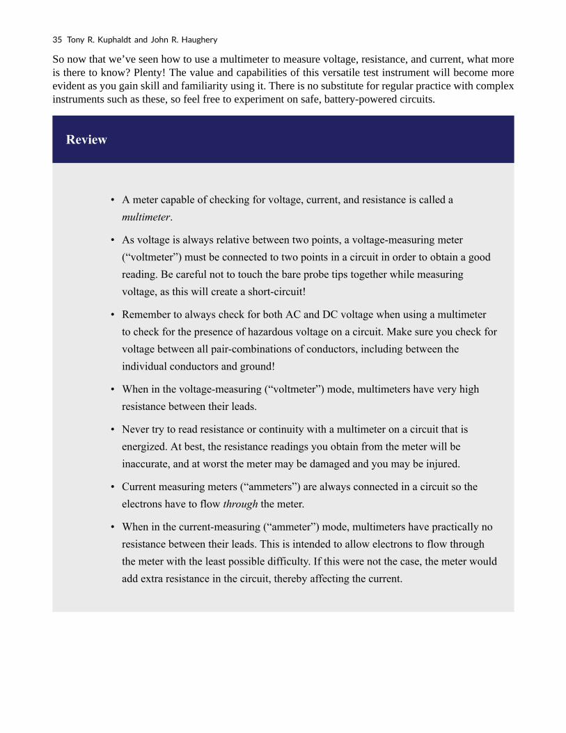
So now that we’ve seen how to use a multimeter to measure voltage, resistance, and current, what more is there to know? Plenty! The value and capabilities of this versatile test instrument will become more evident as you gain skill and familiarity using it. There is no substitute for regular practice with complex instruments such as these, so feel free to experiment on safe, battery-powered circuits.
Review
• A meter capable of checking for voltage, current, and resistance is called a
multimeter.
• As voltage is always relative between two points, a voltage-measuring meter
(“voltmeter”) must be connected to two points in a circuit in order to obtain a good
reading. Be careful not to touch the bare probe tips together while measuring
voltage, as this will create a short-circuit!
• Remember to always check for both AC and DC voltage when using a multimeter
to check for the presence of hazardous voltage on a circuit. Make sure you check for
voltage between all pair-combinations of conductors, including between the
individual conductors and ground!
• When in the voltage-measuring (“voltmeter”) mode, multimeters have very high
resistance between their leads.
• Never try to read resistance or continuity with a multimeter on a circuit that is
energized. At best, the resistance readings you obtain from the meter will be
inaccurate, and at worst the meter may be damaged and you may be injured.
• Current measuring meters (“ammeters”) are always connected in a circuit so the
electrons have to flow through the meter.
• When in the current-measuring (“ammeter”) mode, multimeters have practically no
resistance between their leads. This is intended to allow electrons to flow through
the meter with the least possible difficulty. If this were not the case, the meter would
add extra resistance in the circuit, thereby affecting the current.
35 Tony R. Kuphaldt and John R. Haughery

1.6 Safe Circuit Design
As we saw earlier, a power system with no secure connection to earth ground is unpredictable from a safety perspective. There’s no way to guarantee how much or how little voltage will exist between any point in the circuit and earth ground. By grounding one side of the power system’s voltage source, at least one point in the circuit can be assured to be electrically common with the earth and therefore present no shock hazard. In a simple two-wire electrical power system, the conductor connected to ground is called the neutral, and the other conductor is called the hot, also known as the live or the active:
Figure 1.29 Two wire electrical power system
As far as the voltage source and load are concerned, grounding makes no difference at all. It exists purely for the sake of personal safety, by guaranteeing that at least one point in the circuit will be safe to touch (zero voltage to ground). The “hot” side of the circuit, named for its potential for shock hazard, will be dangerous to touch unless voltage is secured by proper disconnection from the source (ideally, using a systematic lock-out/tag-out procedure).
This imbalance of hazard between the two conductors in a simple power circuit is important to understand. The following series of illustrations are based on common household wiring systems (using DC voltage sources rather than AC for simplicity).
If we take a look at a simple, household electrical appliance such as a toaster with a conductive metal case, we can see that there should be no shock hazard when it is operating properly. The wires conducting power to the toaster’s heating elements are insulated from touching the metal case (and each other) by rubber or plastic.
Applied Industrial Electricity 36

Figure 1.30 No voltage between case and ground
However, if one of the wires inside the toaster were to accidentally come in contact with the metal case, the case will be made electrically common to the wire, and touching the case will be just as hazardous as touching the wire bare. Whether or not this presents a shock hazard depends on which wire accidentally touches:
Figure 1.31 accidental contact voltage between case and ground
If the “hot” wire contacts the case, it places the user of the toaster in danger. On the other hand, if the neutral wire contacts the case, there is no danger of shock:
37 Tony R. Kuphaldt and John R. Haughery

Figure 1.32 Accidental contact no voltage between case and ground
To help ensure that the former failure is less likely than the latter, engineers try to design appliances in such a way as to minimize hot conductor contact with the case. Ideally, of course, you don’t want either wire accidentally coming in contact with the conductive case of the appliance, but there are usually ways to design the layout of the parts to make accidental contact less likely for one wire than for the other.
However, this preventative measure is effective only if the power plug polarity can be guaranteed. If the plug can be reversed, then the conductor more likely to contact the case might very well be the “hot” one:
Figure 1.33 Voltage between case and ground
Appliances designed this way usually come with “polarized” plugs, one prong of the plug being slightly narrower than the other. Power receptacles are also designed like this, one slot being narrower than the other. Consequently, the plug cannot be inserted “backward,” and conductor identity inside the appliance can be guaranteed. Remember that this has no effect whatsoever on the basic function of the appliance: it’s strictly for the sake of user safety.
Some engineers address the safety issue simply by making the outside case of the appliance
Applied Industrial Electricity 38

nonconductive. Such appliances are called double-insulated since the insulating case serves as a second layer of insulation above and beyond that of the conductors themselves. If a wire inside the appliance accidentally comes in contact with the case, there is no danger presented to the user of the appliance.
Other engineers tackle the problem of safety by maintaining a conductive case, but using a third conductor to firmly connect that case to the ground:
Figure 1.34 Ground case zero voltage between case and ground
The third prong on the power cord provides a direct electrical connection from the appliance case to earth ground, making the two points electrically common with each other. If they’re electrically common, then there cannot be any voltage dropped between them. At least, that’s how it is supposed to work. If the hot conductor accidentally touches the metal appliance case, it will create a direct short-circuit back to the voltage source through the ground wire, tripping any overcurrent protection devices. The user of the appliance will remain safe.
This is why it’s so important never to cut the third prong off a power plug when trying to fit it into a two-prong receptacle. If this is done, there will be no grounding of the appliance case to keep the user(s) safe. The appliance will still function properly, but if there is an internal fault bringing the hot wire in contact with the case, the results can be deadly. If a two-prong receptacle must be used, a two-to-three prong receptacle adapter can be installed with a grounding wire attached to the grounded cover screw. This will maintain the safety of the grounded appliance while plugged into this type of receptacle.
Electrically safe engineering doesn’t necessarily end at the load, however. A final safeguard against electrical shock can be arranged on the power supply side of the circuit rather than the appliance itself. This safeguard is called ground-fault detection, and it works like this:
In a properly functioning appliance (shown above), the current measured through the hot conductor should be exactly equal to the current through the neutral conductor, because there’s only one path for
39 Tony R. Kuphaldt and John R. Haughery

electrons to flow in the circuit. With no-fault inside the appliance, there is no connection between circuit conductors and the person touching the case, and therefore no shock.
If, however, the hot wire accidentally contacts the metal case, there will be current through the person touching the case. The presence of a shock current will be manifested as a difference of current between the two power conductors at the receptacle:
Figure 1.35 Difference of current between the two power conductors at the receptacle
This difference in current between the “hot” and “neutral” conductors will only exist if there is current through the ground connection, meaning that there is a fault in the system. Therefore, such a current difference can be used as a way to detect a fault condition. If a device is set up to measure this difference of current between the two power conductors, detection of current imbalance can be used to trigger the opening of a disconnect switch, thus cutting power off and preventing serious shock:
Figure 1.36 Ground fault current interrupters
Such devices are called Ground Fault Current Interrupters, or GFCIs for short. Outside North America, the GFCI is variously known as a safety switch, a residual current device (RCD), an RCBO or RCD/MCB if combined with a miniature circuit breaker, or earth leakage circuit breaker (ELCB). They are
Applied Industrial Electricity 40

compact enough to be built into a power receptacle. These receptacles are easily identified by their distinctive “Test” and “Reset” buttons. The big advantage of using this approach to ensure safety is that it works regardless of the appliance design. Of course, using a double-insulated or grounded appliance in addition to a GFCI receptacle would be better yet, but it’s comforting to know that something can be done to improve safety above and beyond the design and condition of the appliance.
The arc fault circuit interrupter (AFCI), a circuit breaker designed to prevent fires, is designed to open on intermittent resistive short circuits. For example, a normal 15 A breaker is designed to open circuit quickly if loaded well beyond the 15 A rating, more slowly a little beyond the rating. While this protects against direct shorts and several seconds of overload, respectively, it does not protect against arcs– similar to arc-welding. An arc is a highly variable load, repetitively peaking at over 70 A, open circuiting with alternating current zero-crossings. Though the average current is not enough to trip a standard breaker, it is enough to start a fire. This arc could be created by a metallic short circuit which burns the metal open, leaving a resistive sputtering plasma of ionized gases.
The AFCI contains electronic circuitry to sense this intermittent resistive short circuit. It protects against both hot to neutral and hot to ground arcs. The AFCI does not protect against personal shock hazards as a GFCI does. Thus, GFCIs still need to be installed in the kitchen, bath, and outdoors circuits. Since the AFCI often trips upon starting large motors, and more generally on brushed motors, its installation is limited to bedroom circuits by the U.S. National Electrical Code. Use of the AFCI should reduce the number of electrical fires. However, nuisance-trips when running appliances with motors on AFCI circuits is a problem.
Review
• Power systems often have one side of the voltage supply connected to earth ground
to ensure safety at that point.
• The “grounded” conductor in a power system is called the neutral conductor, while
the ungrounded conductor is called the hot.
• Grounding in power systems exists for the sake of personal safety, not the operation
of the load(s).
• The electrical safety of an appliance or other loads can be improved by good
engineering: polarized plugs, double insulation, and three-prong “grounding” plugs
are all ways that safety can be maximized on the load side.
• Ground Fault Current Interrupters (GFCIs) work by sensing a difference in current
between the two conductors supplying power to the load. There should be no
41 Tony R. Kuphaldt and John R. Haughery

difference in current at all. Any difference means that current must be entering or
exiting the load by some means other than the two main conductors, which is not
good. A significant current difference will automatically open a disconnecting
switch mechanism, cutting power off completely.
1.7 Fuses
Normally, the ampacity rating of a conductor is a circuit design limit never to be intentionally exceeded, but there is an application where ampacity exceedance is expected: in the case of fuses.
What is a Fuse?
A fuse is an electrical safety device built around a conductive strip that is designed to melt and separate in the event of excessive current. Fuses are always connected in series with the component(s) to be protected from overcurrent, so that when the fuse blows (opens) it will open the entire circuit and stop current through the component(s). A fuse connected in one branch of a parallel circuit, of course, would not affect current through any of the other branches.
Normally, the thin piece of fuse wire is contained within a safety sheath to minimize hazards of arc blast if the wire burns open with violent force, as can happen in the case of severe overcurrents. In the case of small automotive fuses, the sheath is transparent so that the fusible element can be visually inspected. Residential wiring used to commonly employ screw-in fuses with glass bodies and a thin, narrow metal foil strip in the middle. A photograph showing both types of fuses is shown here:
Applied Industrial Electricity 42

Figure 1.37 Types of fuses
Cartridge type fuses are popular in automotive applications, and in industrial applications when constructed with sheath materials other than glass. Because fuses are designed to “fail” open when their current rating is exceeded, they are typically designed to be replaced easily in a circuit. This means they will be inserted into some type of holder rather than being directly soldered or bolted to the circuit conductors. The following is a photograph showing a couple of glass cartridge fuses in a multi-fuse holder:
43 Tony R. Kuphaldt and John R. Haughery

Figure 1.38 Glass cartridge fuses multi fuse holder
The fuses are held by spring metal clips, the clips themselves being permanently connected to the circuit conductors. The base material of the fuse holder (or fuse block as they are sometimes called) is chosen to be a good insulator.
Another type of fuse holder for cartridge-type fuses is commonly used for installation in equipment control panels, where it is desirable to conceal all electrical contact points from human contact. Unlike the fuse block just shown, where all the metal clips are openly exposed, this type of fuse holder completely encloses the fuse in an insulating housing:
Applied Industrial Electricity 44

Figure 1.39 Fuse holder encloses insulating housing
The most common device in use for overcurrent protection in high-current circuits today is the circuit breaker.
What is a Circuit Breaker?
Circuit breakers are specially designed switches that automatically open to stop current in the event of an overcurrent condition. Small circuit breakers, such as those used in residential, commercial and light industrial service are thermally operated. They contain a bimetallic strip (a thin strip of two metals bonded back-to-back) carrying circuit current, which bends when heated. When enough force is generated by the bimetallic strip (due to overcurrent heating of the strip), the trip mechanism is actuated and the breaker will open. Larger circuit breakers are automatically actuated by the strength
45 Tony R. Kuphaldt and John R. Haughery

of the magnetic field produced by current-carrying conductors within the breaker, or can be triggered to trip by external devices monitoring the circuit current (those devices being called protective relays).
Because circuit breakers don’t fail when subjected to overcurrent conditions—rather, they merely open and can be re-closed by moving a lever—they are more likely to be found connected to a circuit in a more permanent manner than fuses. A photograph of a small circuit breaker is shown here:
Figure 1.40 Small circuit breaker
From outside appearances, it looks like nothing more than a switch. Indeed, it could be used as such. However, its true function is to operate as an overcurrent protection device.
It should be noted that some automobiles use inexpensive devices known as fusible links for overcurrent protection in the battery charging circuit, due to the expense of a properly-rated fuse and holder. A fusible link is a primitive fuse, being nothing more than a short piece of rubber-insulated wire designed to melt open in the event of overcurrent, with no hard sheathing of any kind. Such crude and potentially dangerous devices are never used in industry or even residential power use, mainly due to the greater voltage and current levels encountered. As far as this author is concerned, their application even in automotive circuits is questionable.
The electrical schematic drawing symbol for a fuse is an S-shaped curve:
Applied Industrial Electricity 46

Figure 1.41 S shaped curve
Fuse Ratings
Fuses are primarily rated, as one might expect, in the unit for current: amps. Although their operation depends on the self-generation of heat under conditions of excessive current by means of the fuse’s own electrical resistance, they are engineered to contribute a negligible amount of extra resistance to the circuits they protect. This is largely accomplished by making the fuse wire as short as is practically possible. Just as a normal wire’s ampacity is not related to its length (10-gauge solid copper wire will handle 40 amps of current in free air, regardless of how long or short of a piece it is), a fuse wire of certain material and gauge will blow at a certain current no matter how long it is. Since length is not a factor in current rating, the shorter it can be made, the less resistance it will have end-to-end.
However, the fuse designer also has to consider what happens after a fuse blows: the melted ends of the once-continuous wire will be separated by an air gap, with full supply voltage between the ends. If the fuse isn’t made long enough on a high-voltage circuit, a spark may be able to jump from one of the melted wire ends to the other, completing the circuit again:
47 Tony R. Kuphaldt and John R. Haughery
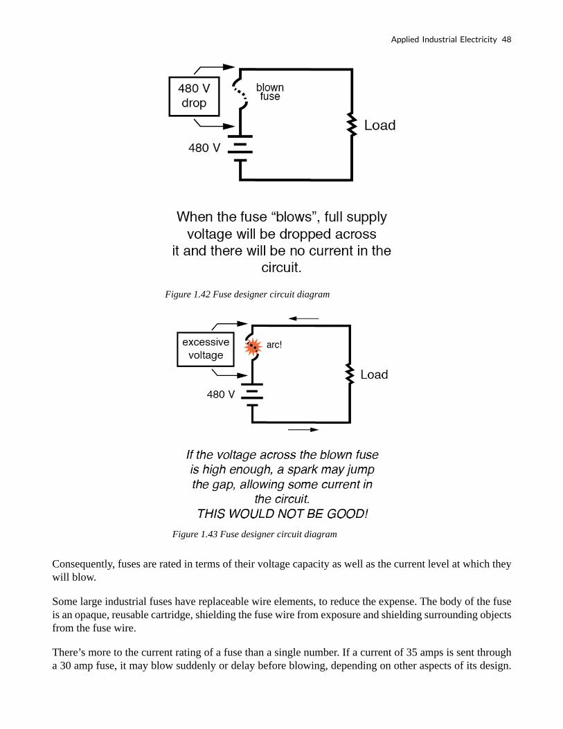
Figure 1.42 Fuse designer circuit diagram
Figure 1.43 Fuse designer circuit diagram
Consequently, fuses are rated in terms of their voltage capacity as well as the current level at which they will blow.
Some large industrial fuses have replaceable wire elements, to reduce the expense. The body of the fuse is an opaque, reusable cartridge, shielding the fuse wire from exposure and shielding surrounding objects from the fuse wire.
There’s more to the current rating of a fuse than a single number. If a current of 35 amps is sent through a 30 amp fuse, it may blow suddenly or delay before blowing, depending on other aspects of its design.
Applied Industrial Electricity 48

Some fuses are intended to blow very fast, while others are designed for more modest “opening” times, or even for a delayed action depending on the application. The latter fuses are sometimes called slow-blow fuses due to their intentional time-delay characteristics.
A classic example of a slow-blow fuse application is in electric motor protection, where inrush currents of up to ten times normal operating current are commonly experienced every time the motor is started from a dead stop. If fast-blowing fuses were to be used in an application like this, the motor could never get started because the normal inrush current levels would blow the fuse(s) immediately! The design of a slow-blow fuse is such that the fuse element has more mass (but no more ampacity) than an equivalent fast-blow fuse, meaning that it will heat up slower (but to the same ultimate temperature) for any given amount of current.
On the other end of the fuse action spectrum, there are so-called semiconductor fuses designed to open very quickly in the event of an overcurrent condition. Semiconductor devices such as transistors tend to be especially intolerant of overcurrent conditions, and as such require fast-acting protection against overcurrents in high-power applications.
Fuses are always supposed to be placed on the “hot” side of the load in systems that are grounded. The intent of this is for the load to be completely de-energized in all respects after the fuse opens. To see the difference between fusing the “hot” side versus the “neutral” side of a load, compare these two circuits:
Figure 1.44 Fuse designer circuit diagram
49 Tony R. Kuphaldt and John R. Haughery

Figure 1.45 Fuse designer circuit diagram
In either case, the fuse successfully interrupted current to the load, but the lower circuit fails to interrupt potentially dangerous voltage from either side of the load to ground, where a person might be standing. The first circuit design is much safer.
As it was said before, fuses are not the only type of overcurrent protection device in use. Switch-like devices called circuit breakers are often (and more commonly) used to open circuits with excessive current, their popularity due to the fact that they don’t destroy themselves in the process of breaking the circuit as fuses do. In any case, though, placement of the overcurrent protection device in a circuit will follow the same general guidelines listed above: namely, to “fuse” the side of the power supply not connected to ground.
Although overcurrent protection placement in a circuit may determine the relative shock hazard of that circuit under various conditions, it must be understood that such devices were never intended to guard against electric shock. Neither fuses nor circuit breakers were designed to open in the event of a person getting shocked; rather, they are intended to open only under conditions of potential conductor overheating. Overcurrent devices primarily protect the conductors of a circuit from overtemperature damage (and the fire hazards associated with overly hot conductors), and secondarily protect specific pieces of equipment such as loads and generators (some fast-acting fuses are designed to protect electronic devices particularly susceptible to current surges). Since the current levels necessary for electric shock or electrocution are much lower than the normal current levels of common power loads, a condition of overcurrent is not indicative of shock occurring. There are other devices designed to detect certain shock conditions (ground-fault detectors being the most popular), but these devices strictly serve that one purpose and are uninvolved with protection of the conductors against overheating.
Applied Industrial Electricity 50

Review
• A fuse is a small, thin conductor designed to melt and separate into two pieces for
the purpose of breaking a circuit in the event of excessive current.
• A circuit breaker is a specially designed switch that automatically opens to interrupt
circuit current in the event of an overcurrent condition. They can be “tripped”
(opened) thermally, by magnetic fields, or by external devices called “protective
relays,” depending on the design of breaker, its size, and the application.
• Fuses are primarily rated in terms of maximum current, but are also rated in terms
of how much voltage drop they will safely withstand after interrupting a circuit.
• Fuses can be designed to blow fast, slow, or anywhere in between for the same
maximum level of current.
• The best place to install a fuse in a grounded power system is on the ungrounded
conductor path to the load. That way, when the fuse blows there will only be the
grounded (safe) conductor still connected to the load, making it safer for people to
be around.
51 Tony R. Kuphaldt and John R. Haughery

2. BASIC CONCEPTS AND RELATIONSHIPS
2.1 Static Electricity
It was discovered centuries ago that certain types of materials would mysteriously attract one another after being rubbed together. For example, after rubbing a piece of silk against a piece of glass, the silk and glass would tend to stick together. Indeed, there was an attractive force that could be demonstrated even when the two materials were separated:
Figure 2.1
Glass and silk aren’t the only materials known to behave like this. Anyone who has ever brushed up against a latex balloon only to find that it tries to stick to them has experienced this same phenomenon. Paraffin wax and wool cloth are another pair of materials early experimenters recognized as manifesting attractive forces after being rubbed together:
Figure 2.2
This phenomenon became even more interesting when it was discovered that identical materials, after having been rubbed with their respective cloths, always repelled each other:
52
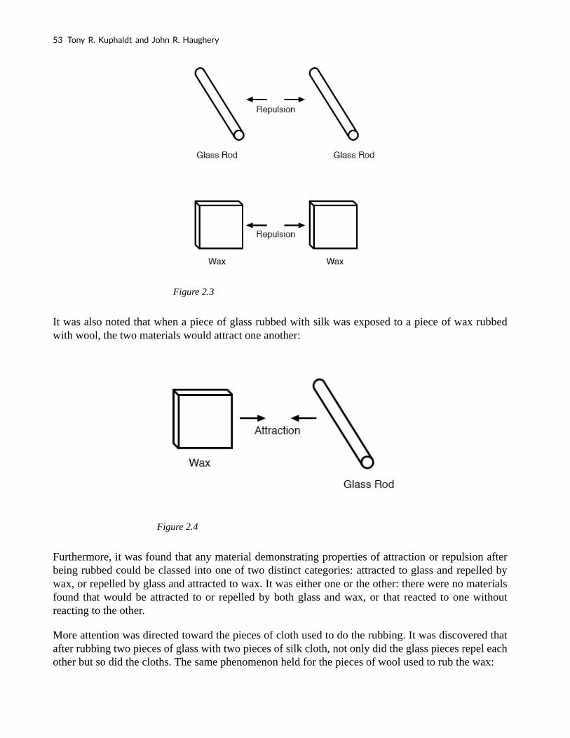
Figure 2.3
It was also noted that when a piece of glass rubbed with silk was exposed to a piece of wax rubbed with wool, the two materials would attract one another:
Figure 2.4
Furthermore, it was found that any material demonstrating properties of attraction or repulsion after being rubbed could be classed into one of two distinct categories: attracted to glass and repelled by wax, or repelled by glass and attracted to wax. It was either one or the other: there were no materials found that would be attracted to or repelled by both glass and wax, or that reacted to one without reacting to the other.
More attention was directed toward the pieces of cloth used to do the rubbing. It was discovered that after rubbing two pieces of glass with two pieces of silk cloth, not only did the glass pieces repel each other but so did the cloths. The same phenomenon held for the pieces of wool used to rub the wax:
53 Tony R. Kuphaldt and John R. Haughery

Figure 2.5
Now, this was really strange to witness. After all, none of these objects were visibly altered by the rubbing, yet they definitely behaved differently than before they were rubbed. Whatever change took place to make these materials attract or repel one another was invisible.
Some experimenters speculated that invisible “fluids” were being transferred from one object to another during the process of rubbing and that these “fluids” were able to effect a physical force over a distance. Charles Dufay was one of the early experimenters who demonstrated that there were definitely two different types of changes wrought by rubbing certain pairs of objects together. The fact that there was more than one type of change manifested in these materials was evident by the fact that there were two types of forces produced: attraction and repulsion. The hypothetical fluid transfer became known as a charge.
One pioneering researcher, Benjamin Franklin, came to the conclusion that there was only one fluid exchanged between rubbed objects, and that the two different “charges” were nothing more than either an excess or a deficiency of that one fluid. After experimenting with wax and wool, Franklin suggested that the coarse wool removed some of this invisible fluid from the smooth wax, causing an excess of fluid on the wool and a deficiency of fluid on the wax. The resulting disparity in fluid content between the wool and wax would then cause an attractive force, as the fluid tried to regain its former balance between the two materials.
Postulating the existence of a single “fluid” that was either gained or lost through rubbing accounted best for the observed behavior: that all these materials fell neatly into one of two categories when rubbed, and most importantly, that the two active materials rubbed against each other always fell into opposing categories as evidenced by their invariable attraction to one another. In other words,
Applied Industrial Electricity 54

there was never a time where two materials rubbed against each other both became either positive or negative.
Following Franklin’s speculation of the wool rubbing something off of the wax, the type of charge that was associated with rubbed wax became known as “negative” (because it was supposed to have a deficiency of fluid) while the type of charge associated with the rubbing wool became known as “positive” (because it was supposed to have an excess of fluid). Little did he know that his innocent conjecture would cause much confusion for students of electricity in the future!
Precise measurements of electrical charges were carried out by the French physicist Charles Coulomb in the 1780s using a device called a torsional balance measuring the force generated between two electrically charged objects. The results of Coulomb’s work led to the development of a unit of electrical charge named in his honor, the coulomb. If two “point” objects (hypothetical objects having no appreciable surface area) were equally charged to a measure of 1 coulomb, and placed 1 meter (approximately 1 yard) apart, they would generate a force of about 9 billion newtons (approximately 2 billion pounds), either attracting or repelling depending on the types of charges involved. The operational definition of a coulomb as the unit of electrical charge (in terms of force generated between point charges) was found to be equal to an excess or deficiency of about 6,250,000,000,000,000,000 electrons. Or, stated in reverse terms, one electron has a charge of about 0.00000000000000000016 coulombs. Being that one electron is the smallest known carrier of electric charge, this last figure of charge for the electron is defined as the elementary charge. It was discovered much later that this “fluid” was actually composed of extremely small bits of matter called electrons, so named in honor of the ancient Greek word for amber: another material exhibiting charged properties when rubbed with a cloth.
The Composition of the Atom
Experimentation has since revealed that all objects are composed of extremely small “building-blocks” known as atoms and that these atoms are in turn composed of smaller components known as particles. The three fundamental particles comprising most atoms are called protons, neutrons, and electrons. Whilst the majority of atoms have a combination of protons, neutrons, and electrons, not all atoms have neutrons; an example is the protium isotope (1H1) of hydrogen (Hydrogen-1) which is the lightest and most common form of hydrogen which only has one proton and one electron. Atoms are far too small to be seen, but if we could look at one, it might appear something like this:
Even though each atom in a piece of material tends to hold together as a unit, there’s actually a lot of empty space between the electrons and the cluster of protons and neutrons residing in the middle.
55 Tony R. Kuphaldt and John R. Haughery

Figure 2.6
This crude model is that of the element carbon, with six protons, six neutrons, and six electrons. In any atom, the protons and neutrons are very tightly bound together, which is an important quality. The tightly-bound clump of protons and neutrons in the center of the atom is called the nucleus, and the number of protons in an atom’s nucleus determines its elemental identity: change the number of protons in an atom’s nucleus, and you change the type of atom that it is. In fact, if you could remove three protons from the nucleus of an atom of lead, you will have achieved the old alchemists’ dream of producing an atom of gold! The tight binding of protons in the nucleus is responsible for the stable identity of chemical elements, and the failure of alchemists to achieve their dream.
Neutrons are much less influential on the chemical character and identity of an atom than protons, although they are just as hard to add to or remove from the nucleus, being so tightly bound. If neutrons are added or gained, the atom will still retain the same chemical identity, but its mass will change slightly and it may acquire strange nuclear properties such as radioactivity.
However, electrons have significantly more freedom to move around in an atom than either protons or neutrons. In fact, they can be knocked out of their respective positions (even leaving the atom entirely!) by far less energy than what it takes to dislodge particles in the nucleus. If this happens, the atom still retains its chemical identity, but an important imbalance occurs. Electrons and protons are unique in the fact that they are attracted to one another over a distance. It is this attraction over distance which causes the attraction between rubbed objects, where electrons are moved away from their original atoms to reside around atoms of another object.
Electrons tend to repel other electrons over a distance, as do protons with other protons. The only reason protons bind together in the nucleus of an atom is because of a much stronger force called the strong nuclear force which has effect only under very short distances. Because of this attraction/repulsion behavior between individual particles, electrons and protons are said to have opposite electric charges. That is, each electron has a negative charge, and each proton a positive charge. In equal numbers within an atom, they counteract each other’s presence so that the net charge within the atom is zero. This is why the picture of a carbon atom has six electrons: to balance out the electric charge of the six protons in the
Applied Industrial Electricity 56
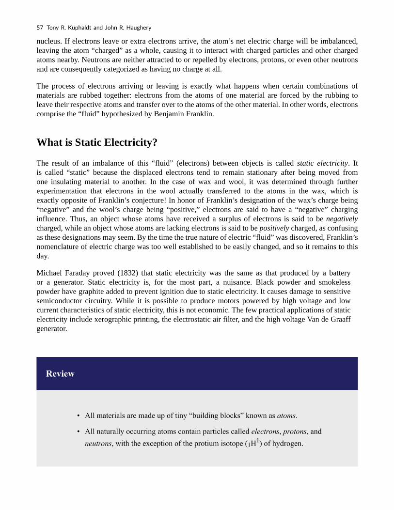
nucleus. If electrons leave or extra electrons arrive, the atom’s net electric charge will be imbalanced, leaving the atom “charged” as a whole, causing it to interact with charged particles and other charged atoms nearby. Neutrons are neither attracted to or repelled by electrons, protons, or even other neutrons and are consequently categorized as having no charge at all.
The process of electrons arriving or leaving is exactly what happens when certain combinations of materials are rubbed together: electrons from the atoms of one material are forced by the rubbing to leave their respective atoms and transfer over to the atoms of the other material. In other words, electrons comprise the “fluid” hypothesized by Benjamin Franklin.
What is Static Electricity?
The result of an imbalance of this “fluid” (electrons) between objects is called static electricity. It is called “static” because the displaced electrons tend to remain stationary after being moved from one insulating material to another. In the case of wax and wool, it was determined through further experimentation that electrons in the wool actually transferred to the atoms in the wax, which is exactly opposite of Franklin’s conjecture! In honor of Franklin’s designation of the wax’s charge being “negative” and the wool’s charge being “positive,” electrons are said to have a “negative” charging influence. Thus, an object whose atoms have received a surplus of electrons is said to be negatively charged, while an object whose atoms are lacking electrons is said to be positively charged, as confusing as these designations may seem. By the time the true nature of electric “fluid” was discovered, Franklin’s nomenclature of electric charge was too well established to be easily changed, and so it remains to this day.
Michael Faraday proved (1832) that static electricity was the same as that produced by a battery or a generator. Static electricity is, for the most part, a nuisance. Black powder and smokeless powder have graphite added to prevent ignition due to static electricity. It causes damage to sensitive semiconductor circuitry. While it is possible to produce motors powered by high voltage and low current characteristics of static electricity, this is not economic. The few practical applications of static electricity include xerographic printing, the electrostatic air filter, and the high voltage Van de Graaff generator.
Review
• All materials are made up of tiny “building blocks” known as atoms.
• All naturally occurring atoms contain particles called electrons, protons, and
neutrons, with the exception of the protium isotope (1H1) of hydrogen.
57 Tony R. Kuphaldt and John R. Haughery

• Electrons have a negative (-) electric charge.
• Protons have a positive (+) electric charge.
• Neutrons have no electric charge.
• Electrons can be dislodged from atoms much easier than protons or neutrons.
• The number of protons in an atom’s nucleus determines its identity as a unique
element.
2.2 Conductors, Insulators, and Electron Flow
The electrons of different types of atoms have different degrees of freedom to move around. With some types of materials, such as metals, the outermost electrons in the atoms are so loosely bound that they chaotically move in the space between the atoms of that material by nothing more than the influence of room-temperature heat energy. Because these virtually unbound electrons are free to leave their respective atoms and float around in the space between adjacent atoms, they are often called free electrons.
Conductors vs Insulators
In other types of materials such as glass, the atoms’ electrons have very little freedom to move around. While external forces such as physical rubbing can force some of these electrons to leave their respective atoms and transfer to the atoms of another material, they do not move between atoms within that material very easily.
This relative mobility of electrons within a material is known as electric conductivity. Conductivity is determined by the types of atoms in a material (the number of protons in each atom’s nucleus determines its chemical identity) and how the atoms are linked together with one another. Materials with high electron mobility (many free electrons) are called conductors, while materials with low electron mobility (few or no free electrons) are called insulators.
Here are a few common examples of conductors and insulators:
Applied Industrial Electricity 58

Conductors Insulators
silver glass
copper rubber
gold oil
aluminum asphalt
iron fiberglass
steel porcelain
brass ceramic
bronze quartz
mercury (dry) cotton
graphite (dry) paper
dirty water (dry) wood
concrete plastic
air
diamond
pure water
It must be understood that not all conductive materials have the same level of conductivity, and not all insulators are equally resistant to electron motion. Electrical conductivity is analogous to the transparency of certain materials to light: materials that easily “conduct” light are called “transparent,” while those that don’t are called “opaque.” However, not all transparent materials are equally conductive to light. Window glass is better than most plastics, and certainly better than “clear” fiberglass. So it is with electrical conductors, some being better than others.
For instance, silver is the best conductor in the “conductors” list, offering easier passage for electrons than any other material cited. Dirty water and concrete are also listed as conductors, but these materials are substantially less conductive than any metal.
It should also be understood that some materials experience changes in their electrical properties under different conditions. Glass, for instance, is a very good insulator at room temperature but becomes a conductor when heated to a very high temperature. Gases such as air, normally insulating materials, also become conductive if heated to very high temperatures. Most metals become poorer conductors when heated, and better conductors when cooled. Many conductive materials become perfectly conductive (this is called superconductivity) at extremely low temperatures.
59 Tony R. Kuphaldt and John R. Haughery

Electron Flow / Electric Current
While the normal motion of “free” electrons in a conductor is random, with no particular direction or speed, electrons can be influenced to move in a coordinated fashion through a conductive material. This uniform motion of electrons is what we call electricity or electric current. To be more precise, it could be called dynamic electricity in contrast to static electricity, which is an unmoving accumulation of electric charge. Just like water flowing through the emptiness of a pipe, electrons are able to move within the empty space within and between the atoms of a conductor. The conductor may appear to be solid to our eyes, but any material composed of atoms is mostly empty space! The liquid-flow analogy is so fitting that the motion of electrons through a conductor is often referred to as a “flow.”
A noteworthy observation may be made here. As each electron moves uniformly through a conductor, it pushes on the one ahead of it, such that all the electrons move together as a group. The starting and stopping of electron flow through the length of a conductive path is virtually instantaneous from one end of a conductor to the other, even though the motion of each electron may be very slow. An approximate analogy is that of a tube filled end-to-end with marbles:
Figure 2.7
The tube is full of marbles, just as a conductor is full of free electrons ready to be moved by an outside influence. If a single marble is suddenly inserted into this full tube on the left-hand side, another marble will immediately try to exit the tube on the right. Even though each marble only traveled a short distance, the transfer of motion through the tube is virtually instantaneous from the left end to the right end, no matter how long the tube is. With electricity, the overall effect from one end of a conductor to the other happens at the speed of light: a swift 186,000 miles per second!!! Each individual electron, though, travels through the conductor at a much slower pace.
Electron Flow Through Wire
If we want electrons to flow in a certain direction to a certain place, we must provide the proper path for them to move, just as a plumber must install piping to get water to flow where he or she wants it to flow. To facilitate this, wires are made of highly conductive metals such as copper or aluminum in a wide variety of sizes.
Remember that electrons can flow only when they have the opportunity to move in the space between the atoms of a material. This means that there can be electric current only where there exists a continuous path of conductive material providing a conduit for electrons to travel through. In the marble analogy, marbles can flow into the left-hand side of the tube (and, consequently, through the
Applied Industrial Electricity 60

tube) if and only if the tube is open on the right-hand side for marbles to flow out. If the tube is blocked on the right-hand side, the marbles will just “pile up” inside the tube, and marble “flow” will not occur. The same holds true for electric current: the continuous flow of electrons requires there be an unbroken path to permit that flow. Let’s look at a diagram to illustrate how this works:
Figure 2.8
A thin, solid line (as shown above) is the conventional symbol for a continuous piece of wire. Since the wire is made of a conductive material, such as copper, its constituent atoms have many free electrons which can easily move through the wire. However, there will never be a continuous or uniform flow of electrons within this wire unless they have a place to come from and a place to go. Let’s add a hypothetical electron “Source” and “Destination:”
Figure 2.9
Now, with the Electron Source pushing new electrons into the wire on the left-hand side, electron flow through the wire can occur (as indicated by the arrows pointing from left to right). However, the flow will be interrupted if the conductive path formed by the wire is broken:
Figure 2.10
Electrical Continuity
Since air is an insulating material, and an air gap separates the two pieces of wire, the once-continuous path has now been broken, and electrons cannot flow from Source to Destination. This is like cutting a water pipe in two and capping off the broken ends of the pipe: water can’t flow if there’s no exit out of the pipe. In electrical terms, we had a condition of electrical continuity when the wire was in one piece, and now that continuity is broken with the wire cut and separated.
61 Tony R. Kuphaldt and John R. Haughery

If we were to take another piece of wire leading to the Destination and simply make physical contact with the wire leading to the Source, we would once again have a continuous path for electrons to flow. The two dots in the diagram indicate physical (metal-to-metal) contact between the wire pieces:
Figure 2.11
Now, we have continuity from the Source, to the newly-made connection, down, to the right, and up to the Destination. This is analogous to putting a “tee” fitting in one of the capped-off pipes and directing water through a new segment of pipe to its destination. Please take note that the broken segment of wire on the right-hand side has no electrons flowing through it because it is no longer part of a complete path from Source to Destination.
It is interesting to note that no “wear” occurs within wires due to this electric current, unlike water-carrying pipes which are eventually corroded and worn by prolonged flows. Electrons do encounter some degree of friction as they move, however, and this friction can generate heat in a conductor. This is a topic we’ll explore in much greater detail later.
Review
• In conductive materials, the outer electrons in each atom can easily come or go and
are called free electrons.
• In insulating materials, the outer electrons are not so free to move.
• All metals are electrically conductive.
• Dynamic electricity, or electric current, is the uniform motion of electrons through a
conductor.
• Static electricity is unmoving (if on an insulator), accumulated charge formed by
either an excess or deficiency of electrons in an object. It is typically formed by
Applied Industrial Electricity 62

charge separation by contact and separation of dissimilar materials.
• For electrons to flow continuously (indefinitely) through a conductor, there must be
a complete, unbroken path for them to move both into and out of that conductor.
2.3 What Are Electric Circuits?
You might have been wondering how charges can continuously flow in a uniform direction through wires without the benefit of these hypothetical Sources and Destinations. In order for the Source-and-Destination scheme to work, both would have to have an infinite capacity for charges in order to sustain a continuous flow!
Using the marble-and-tube analogy from the previous section on conductors, insulators, and electron flow, the marble source, and marble destination buckets would have to be infinitely large to contain enough marble capacity for a “flow” of marbles to be sustained.
What Is a Circuit?
The answer to this paradox is found in the concept of a circuit: a never-ending looped pathway for charge carriers. If we take a wire, or many wires, joined end-to-end, and loop it around so that it forms a continuous pathway, we have the means to support a uniform flow of charge without having to resort to infinite Sources and Destinations:
Figure 2.12
63 Tony R. Kuphaldt and John R. Haughery

Each charge carrier advancing clockwise in this circuit pushes on the one in front of it, which pushes on the one in front of it, and so on, and so on, just like a hula-hoop filled with marbles. Now, we have the capability of supporting a continuous flow of charge indefinitely without the need for infinite supplies and dumps. All we need to maintain this flow is a continuous means of motivation for those charge carriers, which we’ll address in the next section of this chapter on voltage and current.
What Does it mean when a Circuit is broken?
Continuity is just as important in a circuit as it is in a straight piece of wire. Just as in the example with the straight piece of wire between the Source and Destination, any break in this circuit will prevent charge from flowing through it:
Figure 2.13
An important principle to realize here is that it doesn’t matter where the break occurs. Any discontinuity in the circuit will prevent charge flow throughout the entire circuit. Unless there is a continuous, unbroken loop of conductive material for charge carriers to flow through, a sustained flow simply cannot be maintained.
Applied Industrial Electricity 64

Figure 2.14
Review
• A circuit is an unbroken loop of conductive material that allows charge carriers to
flow through continuously without beginning or end.
• If a circuit is “broken,” that means its conductive elements no longer form a complete
path, and continuous charge flow cannot occur in it.
• The location of a break in a circuit is irrelevant to its inability to sustain continuous
charge flow. Any break, anywhere in a circuit prevents the flow of charge carriers
throughout the circuit.
2.4 Voltage and Current
As was previously mentioned, we need more than just a continuous path (i.e., a circuit) before a continuous flow of charge will occur: we also need some means to push these charge carriers around the circuit. Just like marbles in a tube or water in a pipe, it takes some kind of influencing force to initiate flow. With electrons, this force is the same force at work in static electricity: the force produced by an imbalance of electric charge.
If we take the examples of wax and wool which have been rubbed together, we find that the surplus of
65 Tony R. Kuphaldt and John R. Haughery

electrons in the wax (negative charge) and the deficit of electrons in the wool (positive charge) creates an imbalance of charge between them. This imbalance manifests itself as an attractive force between the two objects:
Figure 2.15
If a conductive wire is placed between the charged wax and wool, electrons will flow through it, as some of the excess electrons in the wax rush through the wire to get back to the wool, filling the deficiency of electrons there:
Figure 2.16
The imbalance of electrons between the atoms in the wax and the atoms in the wool creates a force between the two materials. With no path for electrons to flow from the wax to the wool, all this force can do is attract the two objects together.
Now that a conductor bridges the insulating gap, however, the force will provoke electrons to flow in a uniform direction through the wire, if only momentarily, until the charge in that area neutralizes and the force between the wax and wool diminishes.
The electric charge formed between these two materials by rubbing them together serves to store a
Applied Industrial Electricity 66

certain amount of energy. This energy is not unlike the energy stored in a high reservoir of water that has been pumped from a lower-level pond:
Figure 2.17
The influence of gravity on the water in the reservoir creates a force that attempts to move the water down to the lower level again. If a suitable pipe is run from the reservoir back to the pond, water will flow under the influence of gravity down from the reservoir, through the pipe:
67 Tony R. Kuphaldt and John R. Haughery
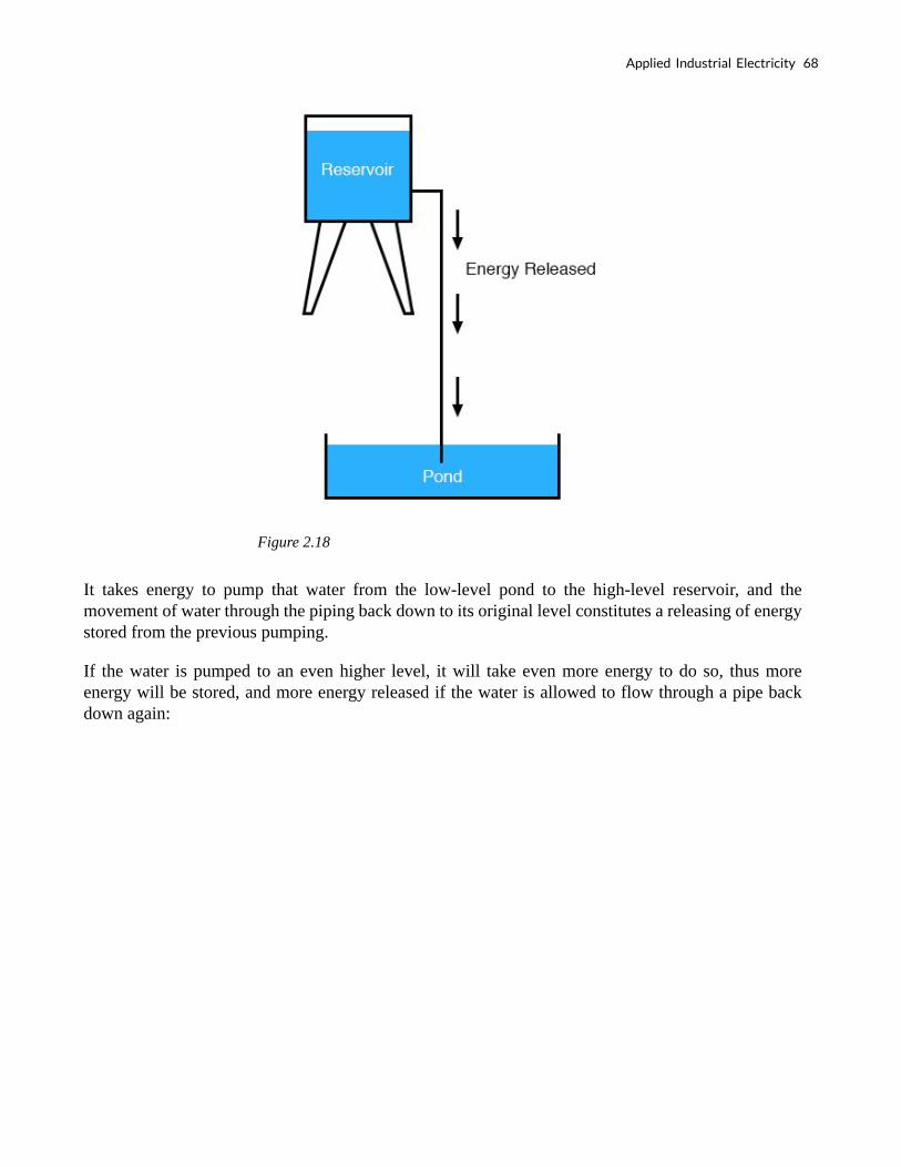
Figure 2.18
It takes energy to pump that water from the low-level pond to the high-level reservoir, and the movement of water through the piping back down to its original level constitutes a releasing of energy stored from the previous pumping.
If the water is pumped to an even higher level, it will take even more energy to do so, thus more energy will be stored, and more energy released if the water is allowed to flow through a pipe back down again:
Applied Industrial Electricity 68

Figure 2.19
Electrons are not much different. If we rub wax and wool together, we “pump” electrons away from their normal “levels,” creating a condition where a force exists between the wax and wool, as the electrons seek to re-establish their former positions (and balance within their respective atoms). The force attracting electrons back to their original positions around the positive nuclei of their atoms is analogous to the force gravity exerts on the water in the reservoir, trying to draw it down to its former level. Just as the pumping of water to a higher level results in energy being stored, “pumping” electrons to create an electric charge imbalance results in a certain amount of energy being stored in that imbalance. And, just as providing a way for water to flow back down from the heights of the reservoir results in a release of that stored energy, providing a way for electrons to flow back to their original “levels” results in a release of stored energy.
When the charge carriers are poised in that static condition (just like water sitting still, high in a reservoir), the energy stored there is called potential energy, because it has the possibility (potential) of release that has not been fully realized yet.
69 Tony R. Kuphaldt and John R. Haughery

Understanding the Concept of Voltage
When the charge carriers are poised in that static condition (just like water sitting still, high in a reservoir), the energy stored there is called potential energy, because it has the possibility (potential) of release that has not been fully realized yet.
When you scuff your rubber-soled shoes against a fabric carpet on a dry day, you create an imbalance of electric charge between yourself and the carpet. The action of scuffing your feet stores energy in the form of an imbalance of charges forced from their original locations. This charge (static electricity) is stationary, and you won’t realize that energy is being stored at all. However, once you place your hand against a metal doorknob (with lots of electron mobility to neutralize your electric charge), that stored energy will be released in the form of a sudden flow of charge through your hand, and you will perceive it as an electric shock!
This potential energy, stored in the form of an electric charge imbalance and capable of provoking charge carriers to flow through a conductor, can be expressed as a term called voltage, which technically is a measure of potential energy per unit charge or something a physicist would call specific potential energy.
The Definition of Voltage
Defined in the context of static electricity, voltage is the measure of work required to move a unit charge from one location to another, against the force which tries to keep electric charges balanced. In the context of electrical power sources, voltage is the amount of potential energy available (work to be done) per unit charge, to move charges through a conductor. Because voltage is an expression of potential energy, representing the possibility or potential for energy release as the charge moves from one “level” to another, it is always referenced between two points. Consider the water reservoir analogy:
Applied Industrial Electricity 70

Figure 2.20
Because of the difference in the height of the drop, there’s potential for much more energy to be released from the reservoir through the piping to location 2 than to location 1. The principle can be intuitively understood in dropping a rock: which results in a more violent impact, a rock dropped from a height of one foot, or the same rock dropped from a height of one mile?
Obviously, the drop of greater height results in greater energy released (a more violent impact). We cannot assess the amount of stored energy in a water reservoir simply by measuring the volume of water any more than we can predict the severity of a falling rock’s impact simply from knowing the weight of the rock: in both cases we must also consider how far these masses will drop from their initial height. The amount of energy released by allowing a mass to drop is relative to the distance between its starting and ending points. Likewise, the potential energy available for moving charge carriers from one point to another is relative to those two points. Therefore, voltage is always expressed as a quantity between two points.
Interestingly enough, the analogy of a mass potentially “dropping” from one height to another is such an apt model that voltage between two points is sometimes called a voltage drop.
Generating Voltage
Voltage can be generated by means other than rubbing certain types of materials against each other. Chemical reactions, radiant energy, and the influence of magnetism on conductors are a few ways in which voltage may be produced. Respective examples of these three sources of voltage are batteries, solar cells, and generators (such as the “alternator” unit under the hood of your automobile). For now, we won’t go into detail as to how each of these voltage sources works—more important is that we understand how voltage sources can be applied to create charge flow in an electric circuit.
Let’s take the symbol for a chemical battery and build a circuit step by step:
71 Tony R. Kuphaldt and John R. Haughery

Figure 2.21
How Do Voltage Sources Work?
Any source of voltage, including batteries, have two points for electrical contact. In this case, we have point 1 and point 2 in the above diagram. The horizontal lines of varying length indicate that this is a battery, and they further indicate the direction in which this battery’s voltage will try to push charge carriers through a circuit. The fact that the horizontal lines in the battery symbol appear separated (and thus unable to serve as a path for charge flow) is no cause for concern: in real life, those horizontal lines represent metallic plates immersed in a liquid or semi-solid material that not only conducts charges but also generates the voltage to push them along by interacting with the plates.
Notice the little “+” and “-” signs to the immediate left of the battery symbol. The negative (-) end of the battery is always the end with the shortest dash, and the positive (+) end of the battery is always the end with the longest dash. The positive end of a battery is the end that tries to push charge carriers out of it (remember that by convention we think of charge carriers as being positively charged, even though electrons are negatively charged). Likewise, the negative end is the end that tries to attract the charge carriers.
With the “+” and “-” ends of the battery not connected to anything, there will be voltage between those two points, but there will be no charge flow through the battery because there is no continuous path through which charge carriers can move.
Applied Industrial Electricity 72

Figure 2.22
The same principle holds true for the water reservoir and pump analogy: without a return pipe back to the pond, stored energy in the reservoir cannot be released in the form of water flow. Once the reservoir is completely filled up, no flow can occur, no matter how much pressure the pump may generate. There needs to be a complete path (circuit) for water to flow from the pond to the reservoir, and back to the pond in order for continuous flow to occur.
We can provide such a path for the battery by connecting a piece of wire from one end of the battery to the other. Forming a circuit with a loop of wire, we will initiate a continuous flow of charge in a clockwise direction:
73 Tony R. Kuphaldt and John R. Haughery

Figure 2.23
Understanding the Concept of Electric Current
As long as the battery continues to produce voltage and the continuity of the electrical path isn’t broken, charge carriers will continue to flow in the circuit. Following the metaphor of water moving through a pipe, this continuous, uniform flow of charge through the circuit is called a current. So long as the voltage source keeps “pushing” in the same direction, the charge carriers will continue to move in the same direction in the circuit. This single-direction flow of current is called a Direct Current, or DC. In the second volume of this book series, electric circuits are explored where the direction of
Applied Industrial Electricity 74

current switches back and forth: Alternating Current, or AC. But for now, we’ll just concern ourselves with DC circuits.
Because electric current is composed of individual charge carriers flowing in unison through a conductor by moving along and pushing on the charge carriers ahead, just like marbles through a tube or water through a pipe, the amount of flow throughout a single circuit will be the same at any point. If we were to monitor a cross-section of the wire in a single circuit, counting the charge carriers flowing by, we would notice the exact same quantity per unit of time as in any other part of the circuit, regardless of conductor length or conductor diameter.
If we break the circuit’s continuity at any point, the electric current will cease in the entire loop, and the full voltage produced by the battery will be manifested across the break, between the wire ends that used to be connected:
Figure 2.24
What is the Polarity of a Voltage Drop?
Notice the “+” and “-” signs drawn at the ends of the break in the circuit, and how they correspond to the “+” and “-” signs next to the battery’s terminals. These markers indicate the direction that the voltage attempts to push the current, that potential direction commonly referred to as polarity. Remember that voltage is always relative between two points. Because of this fact, the polarity of a voltage drop is also relative between two points: whether a point in a circuit gets labeled with a “+” or a “-” depends on the other point to which it is referenced. Take a look at the following circuit, where each corner of the loop is marked with a number for reference:
75 Tony R. Kuphaldt and John R. Haughery

Figure 2.25
With the circuit’s continuity broken between points 2 and 3, the polarity of the voltage dropped between points 2 and 3 is “+” for point 2 and “-” for point 3. The battery’s polarity (1 “+” and 4 “-”) is trying to push the current through the loop clockwise from 1 to 2 to 3 to 4 and back to 1 again.
Now let’s see what happens if we connect points 2 and 3 back together again, but place a break in the circuit between points 3 and 4:
Figure 2.26
With the break between 3 and 4, the polarity of the voltage drop between those two points is “-” for 4 and “+” for 3. Take special note of the fact that point 3’s “sign” is opposite of that in the first example, where the break was between points 2 and 3 (where point 3 was labeled “-”). It is impossible for us to say that point 3 in this circuit will always be either “+” or “-”, because polarity, like voltage itself, is not specific to a single point, but is always relative between two points!
Applied Industrial Electricity 76

Review
• Charge carriers can be motivated to flow through a conductor by the same force
manifested in static electricity.
• Voltage is the measure of specific potential energy (potential energy per unit charge)
between two locations. In layman’s terms, it is the measure of “push” available to
motivate the charge.
• Voltage, as an expression of potential energy, is always relative between two
locations, or points. Sometimes it is called a voltage “drop.”
• When a voltage source is connected to a circuit, the voltage will cause a uniform
flow of charge carriers through that circuit called a current.
• In a single (one loop) circuit, the amount of current at any point is the same as the
amount of current at any other point.
• If a circuit containing a voltage source is broken, the full voltage of that source will
appear across the points of the break.
• The +/- orientation of a voltage drop is called the polarity. It is also relative between
two points.
2.5 Resistance
The circuit in the previous section is not a very practical one. In fact, it can be quite dangerous to build (directly connecting the poles of a voltage source together with a single piece of wire). The reason it is dangerous is that the magnitude of electric current may be very large in such a short circuit, and the release of energy may be very dramatic (usually in the form of heat).
Usually, electric circuits are constructed in such a way as to make practical use of that released energy, in as safe a manner as possible.
77 Tony R. Kuphaldt and John R. Haughery

The Current Flow through Filament of the Lamp
One practical and popular use of electric current is for the operation of electric lighting. The simplest form of electric lamp is a tiny metal “filament” inside of a clear glass bulb, which glows white-hot (“incandesces”) with heat energy when sufficient electric current passes through it. Like the battery, it has two conductive connection points, one for current to enter and the other for current to exit.
Connected to a source of voltage, an electric lamp circuit looks something like this:
Figure 2.27
As the current works its way through the thin metal filament of the lamp, it encounters more opposition to motion than it typically would in a thick piece of wire. This opposition to electric current depends on the type of material, its cross-sectional area, and its temperature. It is technically known as resistance. (It can be said that conductors have low resistance and insulators have very high resistance.) This resistance serves to limit the amount of current through the circuit with a given amount of voltage supplied by the battery, as compared with the “short circuit” where we had nothing but a wire joining one end of the voltage source (battery) to the other.
When the current moves against the opposition of resistance, “friction” is generated. Just like mechanical friction, the friction produced by the current flowing against a resistance manifests itself in the form of heat. The concentrated resistance of a lamp’s filament results in a relatively large amount of heat energy dissipated at that filament. This heat energy is enough to cause the filament to glow white-hot, producing light, whereas the wires connecting the lamp to the battery (which have much lower resistance) hardly even get warm while conducting the same amount of current.
As in the case of the short circuit, if the continuity of the circuit is broken at any point, current flow stops throughout the entire circuit. With a lamp in place, this means that it will stop glowing:
Applied Industrial Electricity 78

Figure 2.28
As before, with no flow of current, the entire potential (voltage) of the battery is available across the break, waiting for the opportunity of a connection to bridge across that break and permit current flow again. This condition is known as an open circuit, where a break in the continuity of the circuit prevents current throughout.
All it takes is a single break in continuity to “open” a circuit. Once any breaks have been connected once again and the continuity of the circuit re-established, it is known as a closed circuit.
The Basis for Switching Lamps
What we see here is the basis for switching lamps on and off by remote switches. Because any break in a circuit’s continuity results in current stopping throughout the entire circuit, we can use a device designed to intentionally break that continuity (called a switch), mounted at any convenient location that we can run wires to, to control the flow of current in the circuit:
Figure 2.29
79 Tony R. Kuphaldt and John R. Haughery

This is how a switch mounted on the wall of a house can control a lamp that is mounted down a long hallway, or even in another room, far away from the switch. The switch itself is constructed of a pair of conductive contacts (usually made of some kind of metal) forced together by a mechanical lever actuator or push button. When the contacts touch each other, the current is able to flow from one to the other and the circuit’s continuity is established. When the contacts are separated, current flow from one to the other is prevented by the insulation of the air between, and the circuit’s continuity is broken.
The Knife Switch
Perhaps the best kind of switch to show for illustration of the basic principle is the “knife” switch:
Figure 2.30
A knife switch is nothing more than a conductive lever, free to pivot on a hinge, coming into physical contact with one or more stationary contact points which are also conductive.
The switch shown in the above illustration is constructed on a porcelain base (an excellent insulating material), using copper (an excellent conductor) for the “blade” and contact points. The handle is plastic to insulate the operator’s hand from the conductive blade of the switch when opening or closing it.
Here is another type of knife switch, with two stationary contacts instead of one:
Applied Industrial Electricity 80

Figure 2.31
The particular knife switch shown here has one “blade” but two stationary contacts, meaning that it can make or break more than one circuit. For now, this is not terribly important to be aware of, just the basic concept of what a switch is and how it works. Knife switches are great for illustrating the basic principle of how a switch works, but they present distinct safety problems when used in high-power electric circuits. The exposed conductors in a knife switch make accidental contact with the circuit a distinct possibility, and any sparking that may occur between the moving blade and the stationary contact is free to ignite any nearby flammable materials. Most modern switch designs have their moving conductors and contact points sealed inside an insulating case in order to mitigate these hazards. A photograph of a few modern switch types show how the switching mechanisms are much more concealed than with the knife design:
81 Tony R. Kuphaldt and John R. Haughery

Figure 2.32
Opened and Closed Circuits
In keeping with the “open” and “closed” terminology of circuits, a switch that is making contact from one connection terminal to the other (example: a knife switch with the blade fully touching the stationary contact point) provides continuity for current to flow through and is called a closed switch.
Conversely, a switch that is breaking continuity (example: a knife switch with the blade not touching the stationary contact point) won’t allow current to pass through and is called an open switch. This terminology is often confusing to the new student of electronics because the words “open” and “closed” are commonly understood in the context of a door, where “open” is equated with free passage and “closed” with blockage. With electrical switches, these terms have opposite meanings: “open” means no flow while “closed” means free passage of electric current.
Review
Applied Industrial Electricity 82

• Resistance is the measure of opposition to electric current.
• A short circuit is an electric circuit offering little or no resistance to the flow of
current. Short circuits are dangerous with high voltage power sources because the
high currents encountered can cause large amounts of heat energy to be released.
• An open circuit is one where the continuity has been broken by an interruption in
the path for current to flow.
• A closed-circuit is one that is complete, with good continuity throughout.
• A device designed to open or close a circuit under controlled conditions is called a
switch.
• The terms “open” and “closed” refer to switches as well as entire circuits. An open
switch is one without continuity: current cannot flow through it. A closed switch is
one that provides a direct (low resistance) path for current to flow through.
2.6 Resistors
Because the relationship between voltage, current, and resistance in any circuit is so regular, we can reliably control any variable in a circuit simply by controlling the other two. Perhaps the easiest variable in any circuit to control is its resistance. This can be done by changing the material, size, and shape of its conductive components (remember how the thin metal filament of a lamp created more electrical resistance than a thick wire?).
What is a Resistor?
Special components called resistors are made for the express purpose of creating a precise quantity of resistance for insertion into a circuit. They are typically constructed of metal wire or carbon and engineered to maintain a stable resistance value over a wide range of environmental conditions. Unlike lamps, they do not produce light, but they do produce heat as electric power is dissipated by them in a working circuit. Typically, though, the purpose of a resistor is not to produce usable heat, but simply to provide a precise quantity of electrical resistance.
83 Tony R. Kuphaldt and John R. Haughery

Resistor Schematic Symbols and Values
The most common schematic symbol for a resistor is a zig-zag line:
Figure 2.33
Resistor values in ohms are usually shown as an adjacent number, and if several resistors are present in a circuit, they will be labeled with a unique identifier number such as R1, R2, R3, etc. As you can see, resistor symbols can be shown either horizontally or vertically:
Figure 2.34
Real resistors look nothing like the zig-zag symbol. Instead, they look like small tubes or cylinders with two wires protruding for connection to a circuit. Here is a sampling of different kinds and sizes of resistors:
Applied Industrial Electricity 84

Figure 2.35
In keeping more with their physical appearance, an alternative schematic symbol for a resistor looks like a small, rectangular box:
Figure 2.36
Resistors can also be shown to have varying rather than fixed resistances. This might be for the purpose of describing an actual physical device designed for the purpose of providing an adjustable resistance, or it could be to show some component that just happens to have an unstable resistance:
85 Tony R. Kuphaldt and John R. Haughery

Figure 2.37
In fact, any time you see a component symbol drawn with a diagonal arrow through it, that component has a variable rather than a fixed value. This symbol “modifier” (the diagonal arrow) is a standard electronic symbol convention.
Variable Resistors
Variable resistors must have some physical means of adjustment, either a rotating shaft or lever that can be moved to vary the amount of electrical resistance. Here is a photograph showing some devices called potentiometers, which can be used as variable resistors:
Applied Industrial Electricity 86

Figure 2.38
Power Rating of Resistors
Because resistors dissipate heat energy as the electric currents through them overcome the “friction” of their resistance, resistors are also rated in terms of how much heat energy they can dissipate without overheating and sustaining damage. Naturally, this power rating is specified in the physical unit of “watts.” Most resistors found in small electronic devices such as portable radios are rated at 1/4 (0.25) watt or less. The power rating of any resistor is roughly proportional to its physical size. Note in the first resistor photograph how the power ratings relate with size: the bigger the resistor, the higher its power dissipation rating. Also, note how resistances (in ohms) have nothing to do with size!
Although it may seem pointless now to have a device doing nothing but resisting electric current, resistors are extremely useful devices in circuits. Because they are simple and so commonly used throughout the world of electricity and electronics, we’ll spend a considerable amount of time analyzing circuits composed of nothing but resistors and batteries.
How are Resistors Useful?
For a practical illustration of resistors’ usefulness, examine the photograph below. It is a picture of a printed circuit board, or PCB: an assembly made of sandwiched layers of insulating phenolic fiber-board and conductive copper strips, into which components may be inserted and secured by a low-temperature welding process called “soldering.” The various components on this circuit board are identified by printed labels. Resistors are denoted by any label beginning with the letter “R”.
87 Tony R. Kuphaldt and John R. Haughery

Figure 2.39
This particular circuit board is a computer accessory called a “modem,” which allows digital information transfer over telephone lines. There are at least a dozen resistors (all rated at 1/4 watt power dissipation) that can be seen on this modem’s board. Every one of the black rectangles (called “integrated circuits” or “chips”) contain their own array of resistors for their internal functions, as well. Another circuit board example shows resistors packaged in even smaller units, called “surface mount devices.” This particular circuit board is the underside of a personal computer hard disk drive, and once again the resistors soldered onto it are designated with labels beginning with the letter “R”:
Applied Industrial Electricity 88

Figure 2.40
There are over one hundred surface-mount resistors on this circuit board, and this count, of course, does not include the number of resistors internal to the black “chips.” These two photographs should convince anyone that resistors—devices that “merely” oppose the flow of electric current—are very important components in the realm of electronics!
“Load” on Schematic Diagrams
In schematic diagrams, resistor symbols are sometimes used to illustrate any general type of device in a circuit doing something useful with electrical energy. Any non-specific electrical device is generally called a load, so if you see a schematic diagram showing a resistor symbol labeled “load,” especially in a tutorial circuit diagram explaining some concept unrelated to the actual use of electrical power, that symbol may just be a kind of shorthand representation of something else more practical than a resistor.
Analyzing Resistor Circuits
To summarize what we’ve learned in this lesson, let’s analyze the following circuit, determining all that we can from the information given:
89 Tony R. Kuphaldt and John R. Haughery

Figure 2.41
All we’ve been given here to start with is the battery voltage (10 volts) and the circuit current (2 amps). We don’t know the resistor’s resistance in ohms or the power dissipated by it in watts. Surveying our array of Ohm’s Law equations, we find two equations that give us answers from known quantities of voltage and current:
Ohm’s Law
Power Equation
Applied Industrial Electricity 90

Example 2.1
Inserting the known quantities of voltage (E) and current (I) into these two equations, we can
determine circuit resistance (R) and power dissipation (P):
Ohm’s Law:
Power Law:
For the circuit conditions of 10 volts and 2 amps, the resistor’s resistance must be 5 Ω. If we were designing a circuit to operate at these values, we would have to specify a resistor with a minimum power rating of 20 watts, or else it would overheat and fail.
Resistor Materials
Resistors can be found in a variety of different materials, each one with its own properties and specific areas of use. Most electrical engineers use the types found below:
Wire wound (WW) Resistors
Wire Wound Resistors are manufactured by winding resistance wire around a non-conductive core in a spiral. They are typically produced for high precision and power applications. The core is usually made of ceramic or fiberglass and the resistance wire is made of nickel-chromium alloy and is not suitable for applications with frequencies higher than 50kHz. Low noise and stability with respect to temperature variations are standard characteristics of Wire Wound Resistors. Resistance values are available from 0.1 up to 100 kW, with accuracies between 0.1% and 20%.
91 Tony R. Kuphaldt and John R. Haughery

Metal Film Resistors
Nichrome or tantalum nitride is typically used for metal film resistors. A combination of a ceramic material and a metal typically make up the resistive material. The resistance value is changed by cutting a spiral pattern in the film, much like a carbon film with a laser or abrasive. Metal film resistors are usually less stable over temperature than wire wound resistors but handle higher frequencies better.
Metal Oxide Film Resistors
Metal oxide resistors use metal oxides such as tin oxide, making them slightly different from metal film resistors. These resistors are reliable and stable and operate at higher temperatures than metal film resistors. Because of this, metal oxide film resistors are used in applications that require high endurance.
Foil Resistors
Developed in the 1960s, the foil resistor is still one of the most accurate and stable types of resistors that you’ll find and are used for applications with high precision requirements. A ceramic substrate that has a thin bulk metal foil cemented to it makes up the resistive element. Foil Resistors feature a very low-temperature coefficient of resistance.
Carbon Composition (CCR) Resistors
Until the 1960s Carbon Composition Resistors were the standard for most applications. They are reliable, but not very accurate (their tolerance cannot be better than about 5%). A mixture of fine carbon particles and non-conductive ceramic material are used for the resistive element of CCR Resistors. The substance is molded into the shape of a cylinder and baked. The dimensions of the body and the ratio of carbon to ceramic material determine the resistance value. More carbon used in the process means there will be a lower resistance. CCR resistors are still useful for certain applications because of their ability to withstand high energy pulses, a good example application would be in a power supply.
Carbon Film Resistors
Carbon film resistors have a thin carbon film (with a spiral cut in the film to increase the resistive path) on an insulating cylindrical core. This allows for the resistance value to be more accurate and also increases the resistance value. Carbon film resistors are much more accurate than carbon composition resistors. Special carbon film resistors are used in applications that require high pulse stability.
Applied Industrial Electricity 92

Performance Indicators (KPIs)
The KPIs for each resistor material can be found below:
Characteristic Metal Film
Thick Metal Film
Precision Metal Film
Carbon Composition
Carbon Film
Temp. range -55+125 -55+130 -55+155 -40+105 .55+155
Max. temp. coeff. 100 100 15 1200 250-1000
Vmax 200-350 250 200 350-500 350-500
Noise (μV per volt of applied DC) 0.5 0.1 0.1 4 (100K) 5 (100K)
R Insul. 10000 10000 10000 10000 10000
Solder (change % in resistance value) 0.20% 0.15% 0.02% 2% 0.50%
Damp heat (change % in resistance value) 0.50% 1% 0.50% 15% 3.50%
Shelf life (change % in resistance value) 0.10% 0.10% 0.00% 5% 2%
Full rating (2000h at 70 degC) 1% 1% 0.03% 10% 4%
Review
• Devices called resistors are built to provide precise amounts of resistance in electric
circuits. Resistors are rated both in terms of their resistance (ohms) and their ability
to dissipate heat energy (watts).
• Resistor resistance ratings cannot be determined from the physical size of the
resistor(s) in question, although approximate power ratings can. The larger the
resistor is the more power it can safely dissipate without suffering damage.
• Any device that performs some useful tasks with electric power is generally known
as a load. Sometimes resistor symbols are used in schematic diagrams to designate a
non-specific load, rather than an actual resistor.
93 Tony R. Kuphaldt and John R. Haughery

2.7 Voltage and Current in a Practical Circuit
Because it takes energy to force charge to flow against the opposition of resistance, there will be voltage manifested (or “dropped”) between any points in a circuit with resistance between them.
It is important to note that although the amount of current (i.e., the quantity of charge moving past a given point every second) is uniform in a simple circuit, the amount of voltage (potential energy per unit charge) between different sets of points in a single circuit may vary considerably:
Figure 2.42
Take this circuit as an example. If we label four points in this circuit with the numbers 1, 2, 3, and 4, we will find that the amount of current conducted through the wire between points 1 and 2 is exactly the same as the amount of current conducted through the lamp (between points 2 and 3). This same quantity of current passes through the wire between points 3 and 4, and through the battery (between points 1 and 4).
However, we will find the voltage appearing between any two of these points to be directly proportional to the resistance within the conductive path between those two points, given that the amount of current along any part of the circuit’s path is the same (which, for this simple circuit, it is).
In a normal lamp circuit, the resistance of a lamp will be much greater than the resistance of the connecting wires, so we should expect to see a substantial amount of voltage between points 2 and 3, with very little between points 1 and 2, or between 3 and 4. The voltage between points 1 and 4, of course, will be the full amount of “force” offered by the battery, which will be only slightly greater than the voltage across the lamp (between points 2 and 3).
This, again, is analogous to the water reservoir system:
Applied Industrial Electricity 94

Figure 2.43
Between points 2 and 3, where the falling water is releasing energy at the water-wheel, there is a difference of pressure between the two points, reflecting the opposition to the flow of water through the water-wheel. From point 1 to point 2, or from point 3 to point 4, where water is flowing freely through reservoirs with little opposition, there is little or no difference of pressure (no potential energy). However, the rate of water flow in this continuous system is the same everywhere (assuming the water levels in both pond and reservoir are unchanging): through the pump, through the water-wheel, and through all the pipes.
So it is with simple electric circuits: current flow is the same at every point in the circuit, although voltages may differ between different sets of points
2.8 Ohm’s Law – How Voltage, Current, and Resistance Relate
The first, and perhaps most important, the relationship between current, voltage, and resistance is called Ohm’s Law, discovered by Georg Simon Ohm and published in his 1827 paper, The Galvanic Circuit Investigated Mathematically.
Voltage, Current, and Resistance
An electric circuit is formed when a conductive path is created to allow the electric charge to continuously move. This continuous movement of electric charge through the conductors of a circuit is called a current, and it is often referred to in terms of “flow,” just like the flow of a liquid through a hollow pipe.
The force motivating charge carriers to “flow” in a circuit is called voltage. Voltage is a specific
95 Tony R. Kuphaldt and John R. Haughery

measure of potential energy that is always relative between two points. When we speak of a certain amount of voltage being present in a circuit, we are referring to the measurement of how much potential energy exists to move charge carriers from one particular point in that circuit to another particular point. Without reference to two particular points, the term “voltage” has no meaning.
Current tends to move through the conductors with some degree of friction, or opposition to the motion. This opposition to motion is more properly called resistance. The amount of current in a circuit depends on the amount of voltage and the amount of resistance in the circuit to oppose current flow. Just like voltage, resistance is a quantity relative between two points. For this reason, the quantities of voltage and resistance are often stated as being “between” or “across” two points in a circuit.
Units of Measurement: Volt, Amp, and Ohm
To be able to make meaningful statements about these quantities in circuits, we need to be able to describe their quantities in the same way that we might quantify mass, temperature, volume, length, or any other kind of physical quantity. For mass, we might use the units of “kilogram” or “gram.” For temperature, we might use degrees Fahrenheit or degrees Celsius. Here are the standard units of measurement for electrical current, voltage, and resistance:
Table 2.1
The “symbol” given for each quantity is the standard alphabetical letter used to represent that quantity in an algebraic equation. Standardized letters like these are common in the disciplines of physics and engineering and are internationally recognized. The “unit abbreviation” for each quantity represents the alphabetical symbol used as a shorthand notation for its particular unit of measurement. And, yes, that strange-looking “horseshoe” symbol is the capital Greek letter Ω, just a character in a foreign alphabet (apologies to any Greek readers here).
Each unit of measurement is named after a famous experimenter in electricity: The amp after the Frenchman Andre M. Ampere, the volt after the Italian Alessandro Volta, and the ohm after the German Georg Simon Ohm.
The mathematical symbol for each quantity is meaningful as well. The “R” for resistance and the “V” for voltage are both self-explanatory, whereas “I” for current seems a bit weird. The “I” is thought to have been meant to represent “Intensity” (of charge flow), and the other symbol for voltage, “E,”
Applied Industrial Electricity 96

stands for “Electromotive force.” From what research I’ve been able to do, there seems to be some dispute over the meaning of “I.” The symbols “E” and “V” are interchangeable for the most part, although some texts reserve “E” to represent voltage across a source (such as a battery or generator) and “V” to represent voltage across anything else.
All of these symbols are expressed using capital letters, except in cases where a quantity (especially voltage or current) is described in terms of a brief period of time (called an “instantaneous” value). For example, the voltage of a battery, which is stable over a long period of time, will be symbolized with a capital letter “E,” while the voltage peak of a lightning strike at the very instant it hits a power line would most likely be symbolized with a lower-case letter “e” (or lower-case “v”) to designate that value as being at a single moment in time. This same lower-case convention holds true for current as well, the lower-case letter “i” representing current at some instant in time. Most direct-current (DC) measurements, however, being stable over time, will be symbolized with capital letters.
Coulomb and Electric Charge
One foundational unit of electrical measurement often taught in the beginnings of electronics courses but used infrequently afterward, is the unit of the coulomb, which is a measure of electric charge proportional to the number of electrons in an imbalanced state. One coulomb of charge is equal to 6,250,000,000,000,000,000 electrons. The symbol for electric charge quantity is the capital letter “Q,” with the unit of coulombs abbreviated by the capital letter “C.” It so happens that the unit for current flow, the amp, is equal to 1 coulomb of charge passing by a given point in a circuit in 1 second of time. Cast in these terms, the current is the rate of electric charge motion through a conductor.
As stated before, voltage is the measure of potential energy per unit charge available to motivate current flow from one point to another. Before we can precisely define what a “volt” is, we must understand how to measure this quantity we call “potential energy.” The general metric unit for energy of any kind is the joule, equal to the amount of work performed by a force of 1 newton exerted through a motion of 1 meter (in the same direction). In British units, this is slightly less than 3/4 pound of force exerted over a distance of 1 foot. Put in common terms, it takes about 1 joule of energy to lift a 3/4-pound weight 1 foot off the ground or to drag something a distance of 1 foot using a parallel pulling force of 3/4 pound. Defined in these scientific terms, 1 volt is equal to 1 joule of electric potential energy per (divided by) 1 coulomb of charge. Thus, a 9-volt battery releases 9 joules of energy for every coulomb of charge moved through a circuit.
These units and symbols for electrical quantities will become very important to know as we begin to explore the relationships between them in circuits.
Ohm’s Law Equations
Ohm’s principal discovery was that the amount of electric current through a metal conductor in a circuit is directly proportional to the voltage impressed across it, for any given temperature. Ohm expressed his discovery in the form of a simple equation, describing how voltage, current, and resistance interrelate:
97 Tony R. Kuphaldt and John R. Haughery

In this algebraic expression, voltage (E) is equal to current (I) multiplied by resistance (R). Using algebra techniques, we can manipulate this equation into two variations, solving for I and for R, respectively:
Analyzing Simple Circuits with Ohm’s Law
Let’s see how these equations might work to help us analyze simple circuits:
Figure 2.44
In the above circuit, there is only one source of voltage (the battery, on the left) and only one source of
Applied Industrial Electricity 98
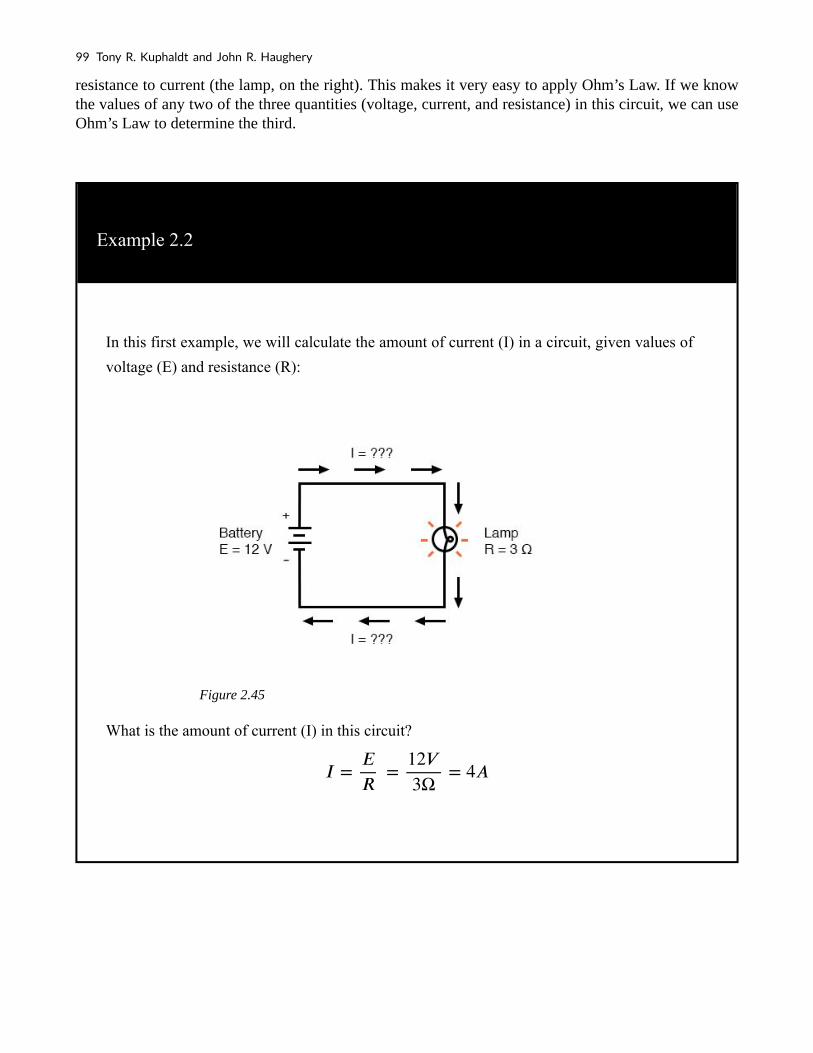
resistance to current (the lamp, on the right). This makes it very easy to apply Ohm’s Law. If we know the values of any two of the three quantities (voltage, current, and resistance) in this circuit, we can use Ohm’s Law to determine the third.
Example 2.2
In this first example, we will calculate the amount of current (I) in a circuit, given values of
voltage (E) and resistance (R):
Figure 2.45
What is the amount of current (I) in this circuit?
99 Tony R. Kuphaldt and John R. Haughery

Example 2.3
In this second example, we will calculate the amount of resistance (R) in a circuit, given
values of voltage (E) and current (I):
What is the amount of resistance (R) offered by the lamp?
Example 2.4
Applied Industrial Electricity 100

In the last example, we will calculate the amount of voltage supplied by a battery, given
values of current (I) and resistance (R):
Figure 2.46
What is the amount of voltage provided by the battery?
Ohm’s Law Triangle Technique
Ohm’s Law is a very simple and useful tool for analyzing electric circuits. It is used so often in the study of electricity and electronics that it needs to be committed to memory by the serious student. For those who are not yet comfortable with algebra, there’s a trick to remembering how to solve for any one quantity, given the other two. First, arrange the letters E, I, and R in a triangle like this:
101 Tony R. Kuphaldt and John R. Haughery

Figure 2.45
If you know E and I, and wish to determine R, just eliminate R from the picture and see what’s left:
Figure 2.46
If you know E and R, and wish to determine I, eliminate I and see what’s left:
Figure 2.47
Lastly, if you know I and R, and wish to determine E, eliminate E and see what’s left:
Figure 2.48
Applied Industrial Electricity 102

Eventually, you’ll have to be familiar with algebra to seriously study electricity and electronics, but this tip can make your first calculations a little easier to remember. If you are comfortable with algebra, all you need to do is commit E = IR to memory and derive the other two formulae from that when you need them!
Review
• Voltage is measured in volts, symbolized by the letters “E” or “V”.
• Current is measured in amps, symbolized by the letter “I”.
• Resistance is measured in ohms, symbolized by the letter “R”.
• ; ;
2.9 Calculating Electric Power
Learn the Power Formula
We’ve seen the formula for determining the power in an electric circuit: by multiplying the voltage in “volts” by the current in “amps” we arrive at an answer in “watts.” Let’s apply this to a circuit example:
Example 2.5
103 Tony R. Kuphaldt and John R. Haughery

In the above circuit, we know we have a battery voltage of 18 volts and a lamp resistance of 3
Ω. Using Ohm’s Law to determine current, we get:
Now that we know the current, we can take that value and multiply it by the voltage to
determine power:
This tells us that the lamp is dissipating (releasing) 108 watts of power, most likely in the
form of both light and heat.
Increasing the Battery’s Voltage
Let’s try taking that same circuit and increasing the battery’s voltage to see what happens. Intuition should tell us that the circuit current will increase as the voltage increases and the lamp resistance stays the same. Likewise, the power will increase as well:
Example 2.6
Applied Industrial Electricity 104

Now, the battery’s voltage is 36 volts instead of 18 volts. The lamp is still providing 3 Ω of
electrical resistance to the flow of current. The current is now:
Example 2.7
This stands to reason: if I = E/R, and we double E while R stays the same, the current should
double. Indeed, it has: we now have 12 amps of current instead of 6. Now, what about power?
105 Tony R. Kuphaldt and John R. Haughery

What does Increasing a Battery’s Voltage do to Power?
Notice that the power has increased just as we might have suspected, but it increased quite a bit more than the current. Why is this? Because power is a function of voltage multiplied by current, and bothvoltage and current doubled from their previous values, the power will increase by a factor of 2 x 2, or 4. You can check this by dividing 432 watts by 108 watts and seeing that the ratio between them is indeed 4.
Using algebra again to manipulate the formula, we can take our original power formula and modify it for applications where we don’t know both voltage and current:
If we only know voltage (E) and resistance (R):
If, and
then, ) or
If we only know current (I) and resistance (R):
If, and
then, or
Joule’s Law Vs. Ohm’s Law
A historical note: it was James Prescott Joule, not Georg Simon Ohm, who first discovered the mathematical relationship between power dissipation and current through a resistance. This discovery, published in 1841, followed the form of the last equation (P = I2R) and is properly known as Joule’s Law. However, these power equations are so commonly associated with the Ohm’s Law equations relating voltage, current, and resistance (E=IR; I=E/R; and R=E/I) that they are frequently credited to Ohm.
Applied Industrial Electricity 106

Power Equations
Review
Power measured in watts, symbolized by the letter “W”.
Joule’s Law:
2.9 Circuit Wiring
So far, we’ve been analyzing single-battery, single-resistor circuits with no regard for the connecting wires between the components, so long as a complete circuit is formed. Does the wire length or circuit “shape” matter to our calculations? Let’s look at a couple of circuit diagrams and find out:
107 Tony R. Kuphaldt and John R. Haughery

Figure 2.49
When we draw wires connecting points in an electric circuit, we usually assume those wires have negligible resistance. As such, they contribute no appreciable effect to the overall resistance of the circuit, and so the only resistance we have to contend with is the resistance in the components. In the above circuits, the only resistance comes from the 5 Ω resistors, so that is all we will consider in our calculations. In real life, metal wires actually do have resistance (and so do power sources!), but those resistances are generally so much smaller than the resistance present in the other circuit components that they can be safely ignored. Exceptions to this rule exist in power system wiring, where even very small amounts of conductor resistance can create significant voltage drops given normal (high) levels of current.
Electrically Common Points in a Circuit
If connecting wire resistance is very little or none, we can regard the connected points in a circuit as being electrically common. That is, points 1 and 2 in the above circuits may be physically joined close together or far apart, and it doesn’t matter for any voltage or resistance measurements relative to those points. The same goes for points 3 and 4. It is as if the ends of the resistor were attached directly across the terminals of the battery, so far as our Ohm’s Law calculations and voltage measurements are concerned. This is useful to know, because it means you can re-draw a circuit diagram or re-wire a circuit, shortening or lengthening the wires as desired without appreciably impacting the circuit’s function. All that matters is that the components attach to each other in the same sequence.
It also means that voltage measurements between sets of “electrically common” points will be the same. That is, the voltage between points 1 and 4 (directly across the battery) will be the same as the voltage between points 2 and 3 (directly across the resistor). Take a close look at the following circuit, and try to determine which points are common to each other:
Applied Industrial Electricity 108

Figure 2.50
Here, we only have 2 components excluding the wires: the battery and the resistor. Though the connecting wires take a convoluted path in forming a complete circuit, there are several electrically common points in the current path. Points 1, 2, and 3 are all common to each other because they’re directly connected together by wire. The same goes for points 4, 5, and 6.
The voltage between points 1 and 6 is 10 volts, coming straight from the battery. However, since points 5 and 4 are common to 6, and points 2 and 3 common to 1, that same 10 volts also exists between these other pairs of points:
• Between points 1 and 4 = 10 volts
• Between points 2 and 4 = 10 volts
• Between points 3 and 4 = 10 volts (directly across the resistor)
• Between points 1 and 5 = 10 volts Between points 2 and 5 = 10 volts
• Between points 3 and 5 = 10 volts Between points 1 and 6 = 10 volts (directly across the battery)
• Between points 2 and 6 = 10 volts Between points 3 and 6 = 10 volts
Since electrically common points are connected together by (zero resistance) wire, there is no significant voltage drop between them regardless of the amount of current conducted from one to the next through that connecting wire. Thus, if we were to read voltages between common points, we should show (practically) zero:
• Between points 1 and 2 = 0 volts
• Points 1, 2, and 3 are Between points 2 and 3 = 0 volts electrically common
• Between points 1 and 3 = 0 volts
• Between points 4 and 5 = 0 volts
• Points 4, 5, and 6 are Between points 5 and 6 = 0 volts electrically common
• Between points 4 and 6 = 0 volts
109 Tony R. Kuphaldt and John R. Haughery

Calculating the Voltage Drop with Ohm’s Law
Example 2.11
This makes sense mathematically, too. With a 10 volt battery and a 5 Ω resistor, the circuit
current will be 2 amps. With wire resistance being zero, the voltage drop across any
continuous stretch of wire can be determined through Ohm’s Law as such:
It should be obvious that the calculated voltage drops across any uninterrupted length of wire in a circuit where the wire is assumed to have zero resistance will always be zero, no matter what the magnitude of current, since zero multiplied by anything equals zero.
Because common points in a circuit will exhibit the same relative voltage and resistance measurements, wires connecting common points are often labeled with the same designation. This is not to say that the terminal connection points are labeled the same, just the connecting wires. Take this circuit as an example:
Applied Industrial Electricity 110

Figure 2.56
Points 1, 2, and 3 are all common to each other, so the wire connecting point 1 to 2 is labeled the same (wire 2) as the wire connecting point 2 to 3 (wire 2). In a real circuit, the wire stretching from point 1 to 2 may not even be the same color or size as the wire connecting point 2 to 3, but they should bear the exact same label. The same goes for the wires connecting points 6, 5, and 4.
Voltage Drop Should Equal Zero in Common Points
Knowing that electrically common points have zero voltage drop between them is a valuable troubleshooting principle. If I measure for voltage between points in a circuit that are supposed to be common to each other, I should read zero. If, however, I read substantial voltage between those two points, then I know with certainty that they cannot be directly connected together. If those points are supposed to be electrically common but they register otherwise, then I know that there is an “open failure” between those points.
Zero Voltage Technically Means Negligible Voltage
One final note: for most practical purposes, wire conductors can be assumed to possess zero resistance from end to end. In reality, however, there will always be some small amount of resistance encountered along the length of a wire, unless it’s a superconducting wire. Knowing this, we need to bear in mind that the principles learned here about electrically common points are all valid to a large degree, but not to an absolute degree. That is, the rule that electrically common points are guaranteed to have zero voltage between them is more accurately stated as such: electrically common points will have very little voltage dropped between them. That small, virtually unavoidable trace of resistance found in any piece of connecting wire is bound to create a small voltage across the length of it as current is conducted through. So long as you understand that these rules are based upon
111 Tony R. Kuphaldt and John R. Haughery

ideal conditions, you won’t be perplexed when you come across some condition appearing to be an exception to the rule.
Review
• Connecting wires in a circuit are assumed to have zero resistance unless otherwise
stated.
• Wires in a circuit can be shortened or lengthened without impacting the circuit’s
function—all that matters is that the components are attached to one another in the
same sequence.
• Points directly connected together in a circuit by zero resistance (wire) are
considered to be electrically common.
• Electrically common points, with zero resistance between them, will have zero
voltage dropped between them, regardless of the magnitude of current (ideally).
• The voltage or resistance readings referenced between sets of electrically common
points will be the same.
• These rules apply to ideal conditions, where connecting wires are assumed to
possess absolutely zero resistance. In real life, this will probably not be the case, but
wire resistances should be low enough so that the general principles stated here still
hold.
Applied Industrial Electricity 112

3. CIRCUIT TOPOLOGY AND LAWS
3.1 Simple Series Circuits
On this page, we’ll outline the three principles you should understand regarding series circuits:
Current: The amount of current is the same through any component in a series circuit.
Resistance: The total resistance of any series circuit is equal to the sum of the individual resistances.
Voltage: The supply voltage in a series circuit is equal to the sum of the individual voltage drops.
Let’s take a look at some examples of series circuits that demonstrate these principles. We’ll start with a series circuit consisting of three resistors and a single battery:
Figure 3.1
The first principle to understand about series circuits is as follows:
The amount of current in a series circuit is the same through any component in the circuit.
Total Series Current
113

This is because there is only one path for current flow in a series circuit. Because electric charge flows through conductors like marbles in a tube, the rate of flow (marble speed) at any point in the circuit (tube) at any specific point in time must be equal.
3.2 Using Ohm’s Law in Series Circuits
From the way that the 9 volt battery is arranged, we can tell that the current in this circuit will flow in a clockwise direction, from point 1 to 2 to 3 to 4 and back to 1. However, we have one source of voltage and three resistances. How do we use Ohm’s Law here?
An important caveat to Ohm’s Law is that all quantities (voltage, current, resistance, and power) must relate to each other in terms of the same two points in a circuit. We can see this concept in action in the single resistor circuit example below.
Using Ohm’s Law in a Simple, Single Resistor Circuit
Example 3.1
With a single-battery, single-resistor circuit, we could easily calculate any quantity because
they all applied to the same two points in the circuit:
Applied Industrial Electricity 114
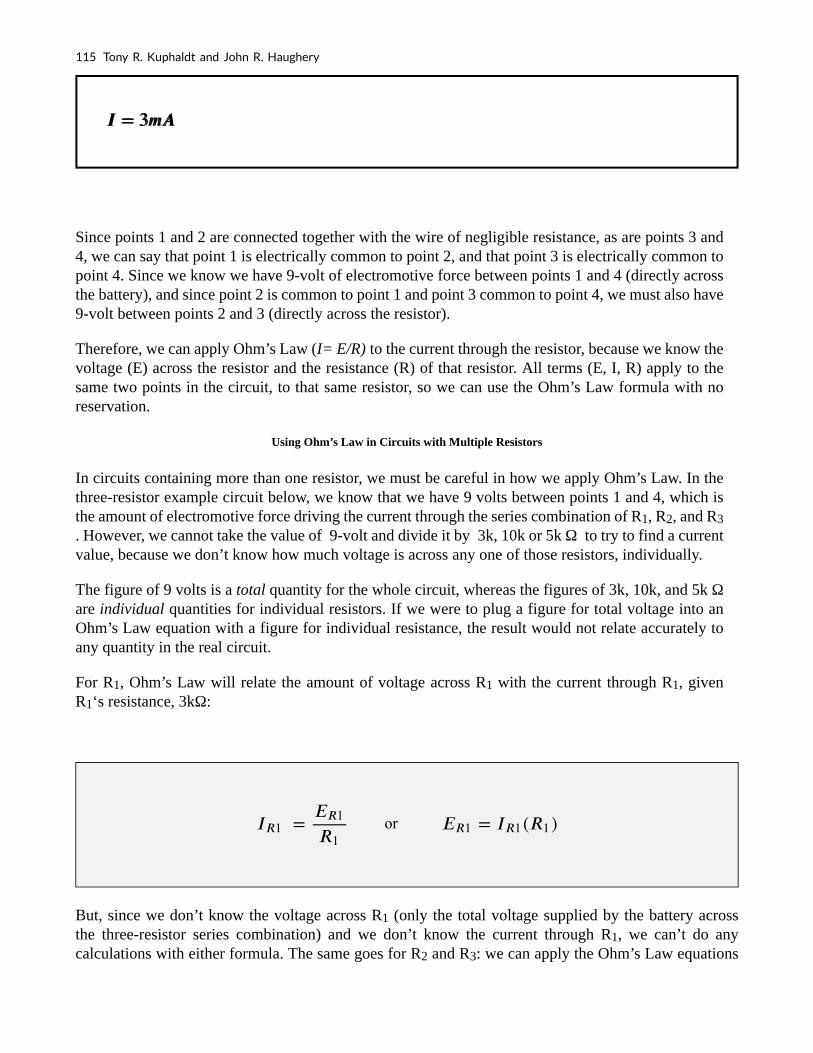
Since points 1 and 2 are connected together with the wire of negligible resistance, as are points 3 and 4, we can say that point 1 is electrically common to point 2, and that point 3 is electrically common to point 4. Since we know we have 9-volt of electromotive force between points 1 and 4 (directly across the battery), and since point 2 is common to point 1 and point 3 common to point 4, we must also have 9-volt between points 2 and 3 (directly across the resistor).
Therefore, we can apply Ohm’s Law (I= E/R) to the current through the resistor, because we know the voltage (E) across the resistor and the resistance (R) of that resistor. All terms (E, I, R) apply to the same two points in the circuit, to that same resistor, so we can use the Ohm’s Law formula with no reservation.
Using Ohm’s Law in Circuits with Multiple Resistors
In circuits containing more than one resistor, we must be careful in how we apply Ohm’s Law. In the three-resistor example circuit below, we know that we have 9 volts between points 1 and 4, which is the amount of electromotive force driving the current through the series combination of R1, R2, and R3 . However, we cannot take the value of 9-volt and divide it by 3k, 10k or 5k Ω to try to find a current value, because we don’t know how much voltage is across any one of those resistors, individually.
The figure of 9 volts is a total quantity for the whole circuit, whereas the figures of 3k, 10k, and 5k Ω are individual quantities for individual resistors. If we were to plug a figure for total voltage into an Ohm’s Law equation with a figure for individual resistance, the result would not relate accurately to any quantity in the real circuit.
For R1, Ohm’s Law will relate the amount of voltage across R1 with the current through R1, given R1‘s resistance, 3kΩ:
or
But, since we don’t know the voltage across R1 (only the total voltage supplied by the battery across the three-resistor series combination) and we don’t know the current through R1, we can’t do any calculations with either formula. The same goes for R2 and R3: we can apply the Ohm’s Law equations
115 Tony R. Kuphaldt and John R. Haughery

if and only if all terms are representative of their respective quantities between the same two points in the circuit.
So what can we do? We know the voltage of the source (9 volts) applied across the series combination of R1, R2, and R3, and we know the resistance of each resistor, but since those quantities aren’t in the same context, we can’t use Ohm’s Law to determine the circuit current. If only we knew what the total resistance was for the circuit: then we could calculate the total current with our figure for total voltage (I=E/R).
Combining Multiple Resistors into an Equivalent Total Resistor
This brings us to the second principle of series circuits:
The total resistance of any series circuit is equal to the sum of the individual resistances.
This should make intuitive sense: the more resistors in series that the current must flow through, the more difficult it will be for the current to flow.
In the example problem, we had a 3 kΩ, 10 kΩ, and 5 kΩ resistors in series, giving us a total resistance of 18 kΩ:
Example 3.2
Applied Industrial Electricity 116

In essence, we’ve calculated the equivalent resistance of R1, R2, and R3 combined. Knowing this, we could redraw the circuit with a single equivalent resistor representing the series combination of R1, R2, and R3:
Calculating Circuit Current Using Ohm’s Law
Now we have all the necessary information to calculate circuit current because we have the voltage between points 1 and 4 (9 volts) and the resistance between points 1 and 4 (18 kΩ):
Example 3.3
117 Tony R. Kuphaldt and John R. Haughery

Calculating Component Voltages Using Ohm’s Law
Knowing that current is equal through all components of a series circuit (and we just determined the current through the battery), we can go back to our original circuit schematic and note the current through each component:
Now that we know the amount of current through each resistor, we can use Ohm’s Law to determine the voltage drop across each one (applying Ohm’s Law in its proper context):
Example 3.4
Applied Industrial Electricity 118

Notice the voltage drops across each resistor, and how the sum of the voltage drops (1.5 + 5 + 2.5) is equal to the battery (supply) voltage: 9 volts.
This is the third principle of series circuits:
The supply voltage in a series circuit is equal to the sum of the individual voltage drops.
119 Tony R. Kuphaldt and John R. Haughery

Total Series Voltage
Analyzing Simple Series Circuits with the “Table Method” and Ohm’s Law
However, the method we just used to analyze this simple series circuit can be streamlined for better understanding. By using a table to list all voltages, currents, and resistance in the circuit, it becomes very easy to see which of those quantities can be properly related in any Ohm’s Law equation:
Table 3.1
The rule with such a table is to apply Ohm’s Law only to the values within each vertical column. For instance, ER1 only with IR1 and R1; ER2 only with IR2 and R2; etc. You begin your analysis by filling in those elements of the table that are given to you from the beginning:
Table 3.2
Applied Industrial Electricity 120

As you can see from the arrangement of the data, we can’t apply the 9 volts of ET (total voltage) to any of the resistances (R1, R2, or R3) in any Ohm’s Law formula because they’re in different columns. The 9 volts of battery voltage is not applied directly across R1, R2, or R3. However, we can use our “rules” of series circuits to fill in blank spots on a horizontal row. In this case, we can use the series rule of resistances to determine a total resistance from the sum of individual resistances:
Table 3.3
Now, with a value for total resistance inserted into the rightmost (“Total”) column, we can apply Ohm’s Law of I=E/R to total voltage and total resistance to arrive at a total current of 500 µA:
Table 3.4
Then, knowing that the current is shared equally by all components of a series circuit (another “rule” of series circuits), we can fill in the currents for each resistor from the current figure just calculated:
121 Tony R. Kuphaldt and John R. Haughery

Table 3.5
Finally, we can use Ohm’s Law to determine the voltage drop across each resistor, one column at a time:
Table 3.6
In summary, a series circuit is defined as having only one path through which current can flow. From this definition, three rules of series circuits follow: all components share the same current; resistances add to equal a larger, total resistance; and voltage drops add to equal a larger, total voltage. All of these rules find root in the definition of a series circuit. If you understand that definition fully, then the rules are nothing more than footnotes to the definition.
Review
• Components in a series circuit share the same current:
• The total resistance in a series circuit is equal to the sum of the individual resistances:
Applied Industrial Electricity 122

• Total voltage in a series circuit is equal to the sum of the individual voltage drops:
3.3 Simple Parallel Circuits
In this section, we’ll outline the three principles you should understand regarding parallel circuits:
Voltage: Voltage is equal across all components in a parallel circuit.
Current: The total circuit current is equal to the sum of the individual branch currents.
Resistance: Individual resistances diminish to equal a smaller total resistance rather than add to make the total.
Let’s take a look at some examples of parallel circuits that demonstrate these principles.
We’ll start with a parallel circuit consisting of three resistors and a single battery:
Figure 3.5
Voltage in Parallel Circuits
The first principle to understand about parallel circuits is that the voltage is equal across all components in the circuit. This is because there are only two sets of electrically common points in a parallel circuit, and the voltage measured between sets of common points must always be the same at any given time.
123 Tony R. Kuphaldt and John R. Haughery
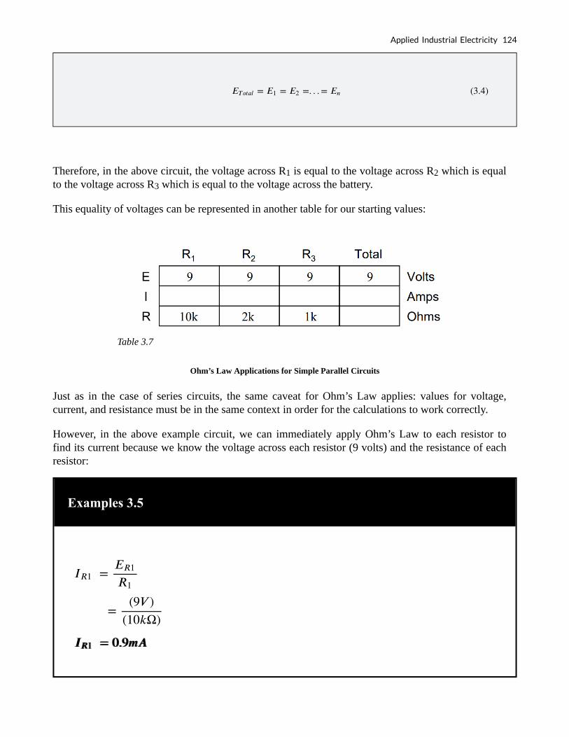
Therefore, in the above circuit, the voltage across R1 is equal to the voltage across R2 which is equal to the voltage across R3 which is equal to the voltage across the battery.
This equality of voltages can be represented in another table for our starting values:
Table 3.7
Ohm’s Law Applications for Simple Parallel Circuits
Just as in the case of series circuits, the same caveat for Ohm’s Law applies: values for voltage, current, and resistance must be in the same context in order for the calculations to work correctly.
However, in the above example circuit, we can immediately apply Ohm’s Law to each resistor to find its current because we know the voltage across each resistor (9 volts) and the resistance of each resistor:
Examples 3.5
Applied Industrial Electricity 124

Table 3.8
At this point, we still don’t know what the total current or total resistance for this parallel circuit is, so we can’t apply Ohm’s Law to the rightmost (“Total”) column. However, if we think carefully about what is happening, it should become apparent that the total current must equal the sum of all individual resistor (“branch”) currents:
125 Tony R. Kuphaldt and John R. Haughery

Figure 3.6
As the total current exits the positive (+) battery terminal at point 1 and travels through the circuit, some of the flow splits off at point 2 to go through R1, some more splits off at point 3 to go through R2, and the remainder goes through R3. Like a river branching into several smaller streams, the combined flow rates of all streams must equal the flow rate of the whole river.
The same thing is encountered where the currents through R1, R2, and R3 join to flow back to the negative terminal of the battery (-) toward point 8: the flow of current from point 7 to point 8 must equal the sum of the (branch) currents through R1, R2, and R3.
This is the second principle of parallel circuits: the total circuit current is equal to the sum of the individual branch currents.
Using this principle, we can fill in the IT spot on our table with the sum of IR1, IR2, and IR3:
Table 3.9
How to Calculate Total Resistance in Parallel Circuits
Finally, applying Ohm’s Law to the rightmost (“Total”) column, we can calculate the total circuit resistance:
Applied Industrial Electricity 126

Table 3.10
The Equation for Resistance in Parallel Circuits
Please note something very important here. The total circuit resistance is only 625 Ω: less than any one of the individual resistors. In the series circuit, where the total resistance was the sum of the individual resistances, the total was bound to be greater than anyone of the resistors individually.
Here in the parallel circuit, however, the opposite is true: we say that the individual resistancesdiminish rather than add to make the total.
This principle completes our triad of “rules” for parallel circuits, just as series circuits were found to have three rules for voltage, current, and resistance.
Mathematically, the relationship between total resistance and individual resistances in a parallel circuit looks like this:
The Equation for Resistance in Parallel Circuits
Three Rules of Parallel Circuits
In summary, a parallel circuit is defined as one where all components are connected between the same
127 Tony R. Kuphaldt and John R. Haughery

set of electrically common points. Another way of saying this is that all components are connected across each other’s terminals.
From this definition, three rules of parallel circuits follow:
All components share the same voltage.
Resistances diminish to equal a smaller, total resistance.
Branch currents add to equal a larger, total current.
Just as in the case of series circuits, all of these rules find root in the definition of a parallel circuit. If you understand that definition fully, then the rules are nothing more than footnotes to the definition.
Review
• Components in a parallel circuit share the same voltage:
• Total resistance in a parallel circuit is less than any of the individual resistances:
• Total current in a parallel circuit is equal to the sum of the individual branch currents:
3.4 Power Calculations
When calculating the power dissipation of resistive components, use any one of the three power equations to derive the answer from values of voltage, current, and/or resistance pertaining to each component:
Applied Industrial Electricity 128

Power Equation
This is easily managed by adding another row to our familiar table of voltages, currents, and resistances:
Table 3.11
Power for any particular table column can be found by the appropriate Ohm’s Law equation (appropriate based on what figures are present for E, I, and R in that column).
An interesting rule for total power versus individual power is that it is additive for any configuration of the circuit: series, parallel, series/parallel, or otherwise. Power is a measure of the rate of work, and since power dissipated must equal the total power applied by the source(s) (as per the Law of Conservation of Energy in physics), circuit configuration has no effect on the mathematics.
Review
129 Tony R. Kuphaldt and John R. Haughery

• Power is additive in any configuration of resistive circuit:
3.5 Correct use of Ohm’s Law
Reminders When Using Ohm’s Law
One of the most common mistakes made by beginning electronics students in their application of Ohm’s Laws is mixing the contexts of voltage, current, and resistance. In other words, a student might mistakenly use a value for I (current) through one resistor and the value for E (voltage) across a set of interconnected resistors, thinking that they’ll arrive at the resistance of that one resistor.
Not so! Remember this important rule: The variables used in Ohm’s Law equations must be common to the same two points in the circuit under consideration. I cannot overemphasize this rule. This is especially important in series-parallel combination circuits where nearby components may have different values for both voltage drop and current.
When using Ohm’s Law to calculate a variable pertaining to a single component, be sure the voltage you’re referencing is sole across that single component and the current you’re referencing is solely through that single component and the resistance you’re referencing is solely for that single component. Likewise, when calculating a variable pertaining to a set of components in a circuit, be sure that the voltage, current, and resistance values are specific to that complete set of components only!
A good way to remember this is to pay close attention to the two points terminating the component or set of components being analyzed, making sure that the voltage in question is across those two points, that the current in question is the flow of electric charge from one of those points all the way to the other point, that the resistance in question is the equivalent of a single resistor between those two points, and that the power in question is the total power dissipated by all components between those two points.
Notes on the “Table” Method of Analyzing Circuits
The “table” method presented for both series and parallel circuits in this chapter is a good way to keep the context of Ohm’s Law correct for any kind of circuit configuration. In a table like the one shown below, you are only allowed to apply an Ohm’s Law equation for the values of a single vertical column at a time:
Applied Industrial Electricity 130

Table 3.12
Deriving values horizontally across columns is allowable as per the principles of series and parallel circuits:
Table 3.13
Table 3.14
Not only does the “table” method simplifies the management of all relevant quantities, but it also facilitates cross-checking of answers by making it easy to solve for the original unknown variables
131 Tony R. Kuphaldt and John R. Haughery

through other methods, or by working backward to solve for the initially given values from your solutions. For example, if you have just solved for all unknown voltages, currents, and resistance in a circuit, you can check your work by adding a row at the bottom for power calculations on each resistor, seeing whether or not all the individual power values add up to the total power. If not, then you must have made a mistake somewhere! While this technique of “cross-checking” your work is nothing new, using the table to arrange all the data for the cross-check(s) results in a minimum of confusion.
Review
• Apply Ohm’s Law to vertical columns in the table.
• Apply rules of series/parallel to horizontal rows in the table.
• Check your calculations by working “backward” to try to arrive at originally given
values (from your first calculated answers), or by solving for a quantity using more
than one method (from different given values).
3.6 Kirchhoff’s Voltage Law (KVL)
What is Kirchhoff’s Voltage Law (KVL)?
The principle known as Kirchhoff’s Voltage Law (discovered in 1847 by Gustav R. Kirchhoff, a German physicist) can be stated as such:
“The algebraic sum of all voltages in a loop must equal zero”
By algebraic, I mean accounting for signs (polarities) as well as magnitudes. By loop, I mean any path traced from one point in a circuit around to other points in that circuit, and finally back to the initial point.
Demonstrating Kirchhoff’s Voltage Law in a Series Circuit
Let’s take another look at our example series circuit, this time numbering the points in the circuit for voltage reference:
Applied Industrial Electricity 132

Figure 3.7
If we were to connect a voltmeter between points 2 and 1, the red test leads to point 2 and the black test lead to point 1, the meter would register +45 volts. Typically, the “+” sign is not shown but rather implied, for positive readings in digital meter displays. However, for this lesson, the polarity of the voltage reading is very important and so I will show positive numbers explicitly: E2-1 = +45V
When a voltage is specified with a double subscript (the characters “2-1” in the notation “E2-1”), it means the voltage at the first point (2) as measured in reference to the second point (1). A voltage specified as “Ecd” would mean the voltage as indicated by a digital meter with the red test lead on point “c” and the black test lead on point “d”: the voltage at “c” in reference to “d”.
Figure 3.8
If we were to take that same voltmeter and measure the voltage drop across each resistor, stepping around the circuit in a clockwise direction with the red test lead of our meter on the point ahead and the black test lead on the point behind, we would obtain the following readings:
133 Tony R. Kuphaldt and John R. Haughery

Figure 3.9
We should already be familiar with the general principle for series circuits stating that individual voltage drops add up to the total applied voltage, but measuring voltage drops in this manner and paying attention to the polarity (mathematical sign) of the readings reveals another facet of this principle: that the voltages measured as such all add up to zero:
Applied Industrial Electricity 134

In the above example, the loop was formed by the following points in this order: 1-2-3-4-1. It doesn’t matter which point we start at or which direction we proceed in tracing the loop; the voltage sum will still equal zero. To demonstrate, we can tally up the voltages in loop 3-2-1-4-3 of the same circuit:
This may make more sense if we re-draw our example series circuit so that all components are represented in a straight line:
Figure 3.10
It’s still the same series circuit, just with the components arranged in a different form. Notice the polarities of the resistor voltage drops with respect to the battery: the battery’s voltage is negative on the left and positive on the right, whereas all the resistor voltage drops are oriented the other way: positive on the left and negative on the right. This is because the resistors are resisting the flow of electric charge being pushed by the battery. In other words, the “push” exerted by the resistors against the flow of electric charge must be in a direction opposite the source of electromotive force.
Here we see what a digital voltmeter would indicate across each component in this circuit, black lead on the left and red lead on the right, as laid out in horizontal fashion:
135 Tony R. Kuphaldt and John R. Haughery

Figure 3.11
If we were to take that same voltmeter and read voltage across combinations of components, starting with the only R1 on the left and progressing across the whole string of components, we will see how the voltages add algebraically (to zero):
Applied Industrial Electricity 136

Figure 3.12
The fact that series voltages add up should be no mystery, but we notice that the polarity of these voltages makes a lot of difference in how the figures add. While reading voltage across R1—R2, and R1—R2—R3(I’m using a “double-dash” symbol “—” to represent the series connection between resistors R1, R2, and R3), we see how the voltages measure successively larger (albeit negative) magnitudes, because the polarities of the individual voltage drops are in the same orientation (positive left, negative right). The sum of the voltage drops across R1, R2, and R3 equals 45 volts, which is the same as the battery’s output, except that the battery’s polarity is opposite that of the resistor voltage drops (negative left, positive right), so we end up with 0 volts measured across the whole string of components.
137 Tony R. Kuphaldt and John R. Haughery

That we should end up with exactly 0 volts across the whole string should be no mystery, either. Looking at the circuit, we can see that the far left of the string (left side of R1: point number 2) is directly connected to the far right of the string (right side of battery: point number 2), as necessary to complete the circuit. Since these two points are directly connected, they are electrically common to each other. And, as such, the voltage between those two electrically common points must be zero.
Demonstrating Kirchhoff’s Voltage Law in a Parallel Circuit
Kirchhoff’s Voltage Law (sometimes denoted as KVL for short) will work for any circuit configuration at all, not just a simple series. Note how it works for this parallel circuit:
Figure 3.13
Being a parallel circuit, the voltage across every resistor is the same as the supply voltage: 6 volts. Tallying up voltages around loop 2-3-4-5-6-7-2, we get:
Note how I label the final (sum) voltage as E2-2. Since we began our loop-stepping sequence at point 2 and ended at point 2, the algebraic sum of those voltages will be the same as the voltage measured between the same point (E2-2), which of course must be zero.
The Validity of Kirchhoff’s Voltage Law, Regardless of Circuit Topology
The fact that this circuit is parallel instead of series has nothing to do with the validity of Kirchhoff’s Voltage Law. For that matter, the circuit could be a “black box”—its component configuration
Applied Industrial Electricity 138

completely hidden from our view, with only a set of exposed terminals for us to measure the voltage between—and KVL would still hold true:
Figure 3.14
Try any order of steps from any terminal in the above diagram, stepping around back to the original terminal, and you’ll find that the algebraic sum of the voltages always equals zero.
Furthermore, the “loop” we trace for KVL doesn’t even have to be a real current path in the closed-circuit sense of the word. All we have to do to comply with KVL is to begin and end at the same point in the circuit, tallying voltage drops and polarities as we go between the next and the last point. Consider this absurd example, tracing “loop” 2-3-6-3-2 in the same parallel resistor circuit:
Figure 3.15
139 Tony R. Kuphaldt and John R. Haughery

Using Kirchhoff’s Voltage Law in a Complex Circuit
KVL can be used to determine an unknown voltage in a complex circuit, where all other voltages around a particular “loop” are known. Take the following complex circuit (actually two series circuits joined by a single wire at the bottom) as an example:
Figure 3.16
To make the problem simpler, I’ve omitted resistance values and simply given voltage drops across each resistor. The two series circuits share a common wire between them (wire 7-8-9-10), making voltage measurements between the two circuits possible.
Example 3.9
If we wanted to determine the voltage between points 4 and 3, we could set up a KVL
equation with the voltage between those points as the unknown:
Applied Industrial Electricity 140

Figure 3.17
141 Tony R. Kuphaldt and John R. Haughery

Figure 3.18
Figure 3.19
Applied Industrial Electricity 142

Figure 3.20
Stepping around the loop 3-4-9-8-3, we write the voltage drop figures as a digital voltmeter would register them, measuring with the red test lead on the point ahead and black test lead on the point behind as we progress around the loop. Therefore, the voltage from point 9 to point 4 is a positive (+) 12 volts because the “red lead” is on point 9 and the “black lead” is on point 4. The voltage from point 3 to point 8 is a positive (+) 20 volts because the “red lead” is on point 3 and the “black lead” is on point 8. The voltage from point 8 to point 9 is zero, of course, because those two points are electrically common.
Our final answer for the voltage from point 4 to point 3 is a negative (-) 32 volts, telling us that point 3 is actually positive with respect to point 4, precisely what a digital voltmeter would indicate with the red lead on point 4 and the black lead on point 3:
143 Tony R. Kuphaldt and John R. Haughery

Figure 3.21
In other words, the initial placement of our “meter leads” in this KVL problem was “backward.” Had we generated our KVL equation starting with E3-4 instead of E4-3, stepping around the same loop with the opposite meter lead orientation, the final answer would have been E3-4 = +32 volts:
Figure 3.22
It is important to realize that neither approach is “wrong.” In both cases, we arrive at the correct
Applied Industrial Electricity 144

assessment of voltage between the two points, 3 and 4: point 3 is positive with respect to point 4, and the voltage between them is 32 volts.
Review
• Kirchhoff’s Voltage Law (KVL): “The algebraic sum of all voltages in a loop must
equal zero”
3.7 Kirchhoff’s Current Law (KCL)
What is Kirchhoff’s Current Law?
Kirchhoff’s Current Law, often shortened to KCL, states that “The algebraic sum of all currents entering and exiting a node must equal zero.”
This law is used to describe how a charge enters and leaves a wire junction point or node on a wire.
Armed with this information, let’s now take a look at an example of the law in practice, why it’s important, and how it was derived.
Parallel Circuit Review
Let’s take a closer look at that last parallel example circuit:
145 Tony R. Kuphaldt and John R. Haughery

Figure 3.23
Table 3.15
Solving for all values of voltage and current in this circuit:
At this point, we know the value of each branch current and of the total current in the circuit. We know that the total current in a parallel circuit must equal the sum of the branch currents, but there’s more going on in this circuit than just that. Taking a look at the currents at each wire junction point (node) in the circuit, we should be able to see something else:
Figure 3.24
Applied Industrial Electricity 146
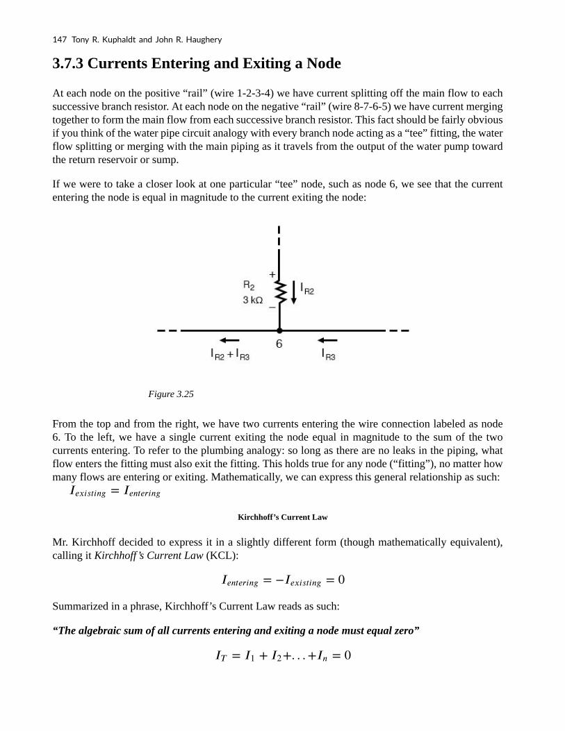
3.7.3 Currents Entering and Exiting a Node
At each node on the positive “rail” (wire 1-2-3-4) we have current splitting off the main flow to each successive branch resistor. At each node on the negative “rail” (wire 8-7-6-5) we have current merging together to form the main flow from each successive branch resistor. This fact should be fairly obvious if you think of the water pipe circuit analogy with every branch node acting as a “tee” fitting, the water flow splitting or merging with the main piping as it travels from the output of the water pump toward the return reservoir or sump.
If we were to take a closer look at one particular “tee” node, such as node 6, we see that the current entering the node is equal in magnitude to the current exiting the node:
Figure 3.25
From the top and from the right, we have two currents entering the wire connection labeled as node 6. To the left, we have a single current exiting the node equal in magnitude to the sum of the two currents entering. To refer to the plumbing analogy: so long as there are no leaks in the piping, what flow enters the fitting must also exit the fitting. This holds true for any node (“fitting”), no matter how many flows are entering or exiting. Mathematically, we can express this general relationship as such:
Kirchhoff’s Current Law
Mr. Kirchhoff decided to express it in a slightly different form (though mathematically equivalent), calling it Kirchhoff’s Current Law (KCL):
Summarized in a phrase, Kirchhoff’s Current Law reads as such:
“The algebraic sum of all currents entering and exiting a node must equal zero”
147 Tony R. Kuphaldt and John R. Haughery

That is, if we assign a mathematical sign (polarity) to each current, denoting whether they enter (+) or exit (-) a node, we can add them together to arrive at a total of zero, guaranteed.
Example 3.10
Taking our example node (number 6), we can determine the magnitude of the current exiting
from the left by setting up a KCL equation with that current as the unknown value:
The negative (-) sign on the value of 5 milliamps tells us that the current is exiting the node, as opposed to the 2 milliamp and 3 milliamp currents, which must both be positive (and therefore entering the node). Whether negative or positive denotes current entering or exiting is entirely arbitrary, so long as they are opposite signs for opposite directions and we stay consistent in our notation, KCL will work.
Together, Kirchhoff’s Voltage and Current Laws are a formidable pair of tools useful in analyzing electric circuits. Their usefulness will become all the more apparent in a later chapter (“Network
Applied Industrial Electricity 148

Analysis”), but suffice it to say that these Laws deserve to be memorized by the electronics student every bit as much as Ohm’s Law.
Review
• Kirchhoff’s Current Law (KCL): “The algebraic sum of all currents entering and
exiting a node must equal zero”
149 Tony R. Kuphaldt and John R. Haughery

4. ALTERNATING CURRENT
4.1 What is Alternating Current (AC)?
Alternating Current
Most students of electricity begin their study with what is known as direct current (DC), which is electricity flowing in a constant direction, and/or possessing a voltage with constant polarity. DC is the kind of electricity made by a battery (with definite positive and negative terminals), or the kind of charge generated by rubbing certain types of materials against each other.
Alternating Current vs Direct Current
As useful and as easy to understand as DC is, it is not the only “kind” of electricity in use. Certain sources of electricity (most notably, rotary electromechanical generators) naturally produce voltages alternating in polarity, reversing positive and negative over time. Either as a voltage switching polarity or as a current switching direction back and forth, this “kind” of electricity is known as Alternating Current (AC):
Figure 4.1 Direct vs alternating current
Whereas the familiar battery symbol is used as a generic symbol for any DC voltage source, the circle with the wavy line inside is the generic symbol for any AC voltage source.
One might wonder why anyone would bother with such a thing as AC. It is true that in some cases AC holds no practical advantage over DC. In applications where electricity is used to dissipate energy in the form of heat, the polarity or direction of current is irrelevant, so long as there is enough voltage and current to the load to produce the desired heat (power dissipation). However, with AC it is possible to
150

build electric generators, motors and power distribution systems that are far more efficient than DC, and so we find AC being used predominantly across the world in high power applications. To explain the details of why this is so, a bit of background knowledge about AC is necessary.
AC Alternators
If a machine is constructed to rotate a magnetic field around a set of stationary wire coils with the turning of a shaft, AC voltage will be produced across the wire coils as that shaft is rotated, in accordance with Faraday’s Law of electromagnetic induction. This is the basic operating principle of an AC generator, also known as an alternator:
Figure 4.2 Alternator operation
Notice how the polarity of the voltage across the wire coils reverses as the opposite poles of the rotating magnet pass by. Connected to a load, this reversing voltage polarity will create a reversing current direction in the circuit. The faster the alternator’s shaft is turned, the faster the magnet will spin, resulting in an alternating voltage and current that switches directions more often in a given amount of time.
While DC generators work on the same general principle of electromagnetic induction, their construction is not as simple as their AC counterparts. With a DC generator, the coil of wire is mounted in the shaft where the magnet is on the AC alternator, and electrical connections are made to this spinning coil via stationary carbon “brushes” contacting copper strips on the rotating shaft. All this is necessary to switch the coil’s changing output polarity to the external circuit so the external circuit sees a constant polarity:
151 Tony R. Kuphaldt and John R. Haughery

Figure 4.3 DC generator operation
The generator shown above will produce two pulses of voltage per revolution of the shaft, both pulses in the same direction (polarity). In order for a DC generator to produce constant voltage, rather than brief pulses of voltage once every 1/2 revolution, there are multiple sets of coils making intermittent contact with the brushes. The diagram shown above is a bit more simplified than what you would see in real life.
The problems involved with making and breaking electrical contact with a moving coil should be obvious (sparking and heat), especially if the shaft of the generator is revolving at high speed. If the atmosphere surrounding the machine contains flammable or explosive vapors, the practical problems of spark-producing brush contacts are even greater. An AC generator (alternator) does not require brushes and commutators to work, and so is immune to these problems experienced by DC generators.
AC Motors
The benefits of AC over DC with regard to generator design are also reflected in electric motors. While DC motors require the use of brushes to make electrical contact with moving coils of wire, AC motors do not. In fact, AC and DC motor designs are very similar to their generator counterparts (identical for the sake of this tutorial), the AC motor being dependent upon the reversing magnetic field produced by alternating current through its stationary coils of wire to rotate the rotating magnet around on its shaft, and the DC motor being dependent on the brush contacts making and breaking connections to reverse current through the rotating coil every 1/2 rotation (180 degrees).
Applied Industrial Electricity 152
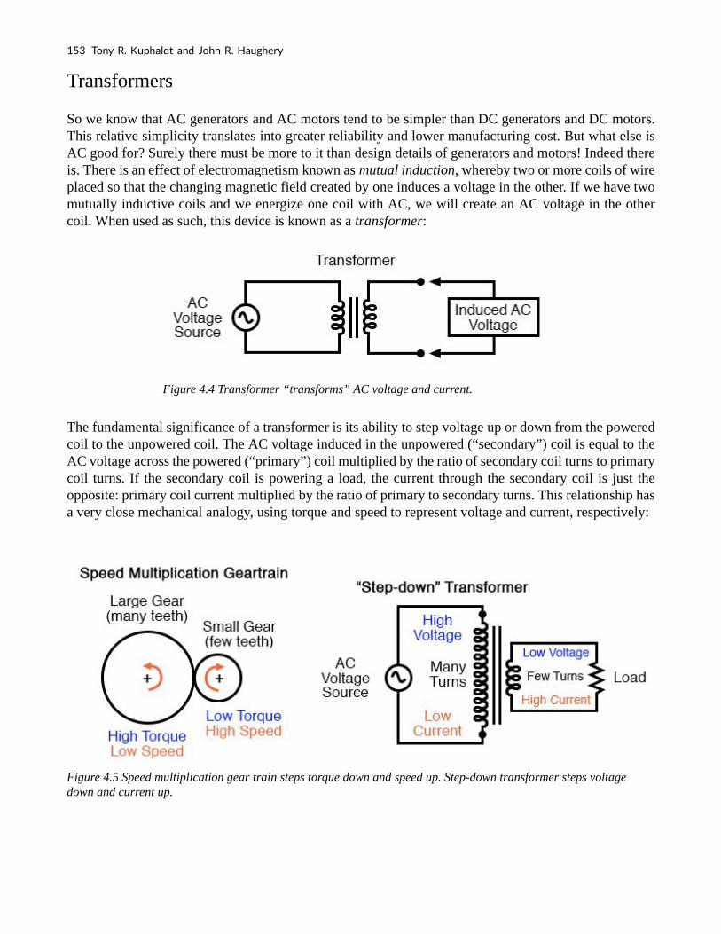
Transformers
So we know that AC generators and AC motors tend to be simpler than DC generators and DC motors. This relative simplicity translates into greater reliability and lower manufacturing cost. But what else is AC good for? Surely there must be more to it than design details of generators and motors! Indeed there is. There is an effect of electromagnetism known as mutual induction, whereby two or more coils of wire placed so that the changing magnetic field created by one induces a voltage in the other. If we have two mutually inductive coils and we energize one coil with AC, we will create an AC voltage in the other coil. When used as such, this device is known as a transformer:
Figure 4.4 Transformer “transforms” AC voltage and current.
The fundamental significance of a transformer is its ability to step voltage up or down from the powered coil to the unpowered coil. The AC voltage induced in the unpowered (“secondary”) coil is equal to the AC voltage across the powered (“primary”) coil multiplied by the ratio of secondary coil turns to primary coil turns. If the secondary coil is powering a load, the current through the secondary coil is just the opposite: primary coil current multiplied by the ratio of primary to secondary turns. This relationship has a very close mechanical analogy, using torque and speed to represent voltage and current, respectively:
Figure 4.5 Speed multiplication gear train steps torque down and speed up. Step-down transformer steps voltage down and current up.
153 Tony R. Kuphaldt and John R. Haughery

If the winding ratio is reversed so that the primary coil has less turns than the secondary coil, the transformer “steps up” the voltage from the source level to a higher level at the load:
Figure 4.6 Speed reduction gear train steps torque up and speed down. Step-up transformer steps voltage up and current down.
The transformer’s ability to step AC voltage up or down with ease gives AC an advantage unmatched by DC in the realm of power distribution in figure below. When transmitting electrical power over long distances, it is far more efficient to do so with stepped-up voltages and stepped-down currents (smaller-diameter wire with less resistive power losses), then step the voltage back down and the current back up for industry, business, or consumer use.
Figure 4.7 Transformers enable efficient long distance high voltage transmission of electric energy.
Transformer technology has made long-range electric power distribution practical. Without the ability
Applied Industrial Electricity 154

to efficiently step voltage up and down, it would be cost-prohibitive to construct power systems for anything but close-range (within a few miles at most) use.
As useful as transformers are, they only work with AC, not DC. Because the phenomenon of mutual inductance relies on changing magnetic fields, and direct current (DC) can only produce steady magnetic fields, transformers simply will not work with direct current. Of course, direct current may be interrupted (pulsed) through the primary winding of a transformer to create a changing magnetic field (as is done in automotive ignition systems to produce high-voltage spark plug power from a low-voltage DC battery), but pulsed DC is not that different from AC. Perhaps more than any other reason, this is why AC finds such widespread application in power systems.
Review
• DC stands for “Direct Current,” meaning voltage or current that maintains constant
polarity or direction, respectively, over time.
• AC stands for “Alternating Current,” meaning voltage or current that changes
polarity or direction, respectively, over time.
• AC electromechanical generators, known as alternators, are of simpler construction
than DC electromechanical generators.
• AC and DC motor design follows respective generator design principles very
closely.
• A transformer is a pair of mutually-inductive coils used to convey AC power from
one coil to the other. Often, the number of turns in each coil is set to create a voltage
increase or decrease from the powered (primary) coil to the unpowered (secondary)
coil.
• Secondary voltage = Primary voltage (secondary turns / primary turns)
• Secondary current = Primary current (primary turns / secondary turns)
155 Tony R. Kuphaldt and John R. Haughery

4.2 Measurements of AC Magnitude
Measurements of AC Magnitude
So far we know that AC voltage alternates in polarity and AC current alternates in direction. We also know that AC can alternate in a variety of different ways, and by tracing the alternation over time we can plot it as a “waveform.” We can measure the rate of alternation by measuring the time it takes for a wave to evolve before it repeats itself (the “period”), and express this as cycles per unit time, or “frequency.” In music, frequency is the same as pitch, which is the essential property distinguishing one note from another.
However, we encounter a measurement problem if we try to express how large or small an AC quantity is. With DC, where quantities of voltage and current are generally stable, we have little trouble expressing how much voltage or current we have in any part of a circuit. But how do you grant a single measurement of magnitude to something that is constantly changing?
Ways of Expressing the Magnitude of an AC Waveform
One way to express the intensity, or magnitude (also called the amplitude), of an AC quantity is to measure its peak height on a waveform graph. This is known as the peak or crest value of an AC waveform:
Figure 4.8 Peak voltage of a waveform.
Another way is to measure the total height between opposite peaks. This is known as the peak-to-peak (P-P) value of an AC waveform:
Applied Industrial Electricity 156

Figure 4.9 Peak-to-peak voltage of a waveform.
Unfortunately, either one of these expressions of waveform amplitude can be misleading when comparing two different types of waves. For example, a square wave peaking at 10 volts is obviously a greater amount of voltage for a greater amount of time than a triangle wave peaking at 10 volts. The effects of these two AC voltages powering a load would be quite different:
Figure 4.10 A square wave produces a greater heating effect than the same peak voltage triangle wave.
One way of expressing the amplitude of different wave shapes in a more equivalent fashion is to mathematically average the values of all the points on a waveform’s graph to a single, aggregate number. This amplitude measurement is known simply as the average value of the waveform. If we average all the points on the waveform algebraically (that is, to consider their sign, either positive or negative), the average value for most waveforms is technically zero, because all the positive points cancel out all the negative points over a full cycle:
157 Tony R. Kuphaldt and John R. Haughery

Figure 4.11 The average value of a sine wave is zero.
This, of course, will be true for any waveform having equal-area portions above and below the “zero” line of a plot. However, as a practical measure of a waveform’s aggregate value, “average” is usually defined as the mathematical mean of all the points’ absolute values over a cycle. In other words, we calculate the practical average value of the waveform by considering all points on the wave as positive quantities, as if the waveform looked like this:
Figure 4.12 Waveform seen by AC “average responding” meter.
Polarity-insensitive mechanical meter movements (meters designed to respond equally to the positive and negative half-cycles of an alternating voltage or current) register in proportion to the waveform’s (practical) average value, because the inertia of the pointer against the tension of the spring naturally averages the force produced by the varying voltage/current values over time. Conversely, polarity-sensitive meter movements vibrate uselessly if exposed to AC voltage or current, their needles oscillating rapidly about the zero mark, indicating the true (algebraic) average value of zero for a symmetrical waveform. When the “average” value of a waveform is referenced in this text, it will be assumed that the “practical” definition of average is intended unless otherwise specified.
Another method of deriving an aggregate value for waveform amplitude is based on the waveform’s
Applied Industrial Electricity 158
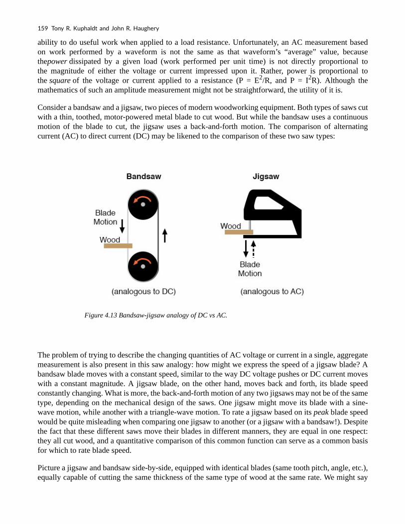
ability to do useful work when applied to a load resistance. Unfortunately, an AC measurement based on work performed by a waveform is not the same as that waveform’s “average” value, because thepower dissipated by a given load (work performed per unit time) is not directly proportional to the magnitude of either the voltage or current impressed upon it. Rather, power is proportional to the square of the voltage or current applied to a resistance (P = E2/R, and P = I2R). Although the mathematics of such an amplitude measurement might not be straightforward, the utility of it is.
Consider a bandsaw and a jigsaw, two pieces of modern woodworking equipment. Both types of saws cut with a thin, toothed, motor-powered metal blade to cut wood. But while the bandsaw uses a continuous motion of the blade to cut, the jigsaw uses a back-and-forth motion. The comparison of alternating current (AC) to direct current (DC) may be likened to the comparison of these two saw types:
Figure 4.13 Bandsaw-jigsaw analogy of DC vs AC.
The problem of trying to describe the changing quantities of AC voltage or current in a single, aggregate measurement is also present in this saw analogy: how might we express the speed of a jigsaw blade? A bandsaw blade moves with a constant speed, similar to the way DC voltage pushes or DC current moves with a constant magnitude. A jigsaw blade, on the other hand, moves back and forth, its blade speed constantly changing. What is more, the back-and-forth motion of any two jigsaws may not be of the same type, depending on the mechanical design of the saws. One jigsaw might move its blade with a sine-wave motion, while another with a triangle-wave motion. To rate a jigsaw based on its peak blade speed would be quite misleading when comparing one jigsaw to another (or a jigsaw with a bandsaw!). Despite the fact that these different saws move their blades in different manners, they are equal in one respect: they all cut wood, and a quantitative comparison of this common function can serve as a common basis for which to rate blade speed.
Picture a jigsaw and bandsaw side-by-side, equipped with identical blades (same tooth pitch, angle, etc.), equally capable of cutting the same thickness of the same type of wood at the same rate. We might say
159 Tony R. Kuphaldt and John R. Haughery
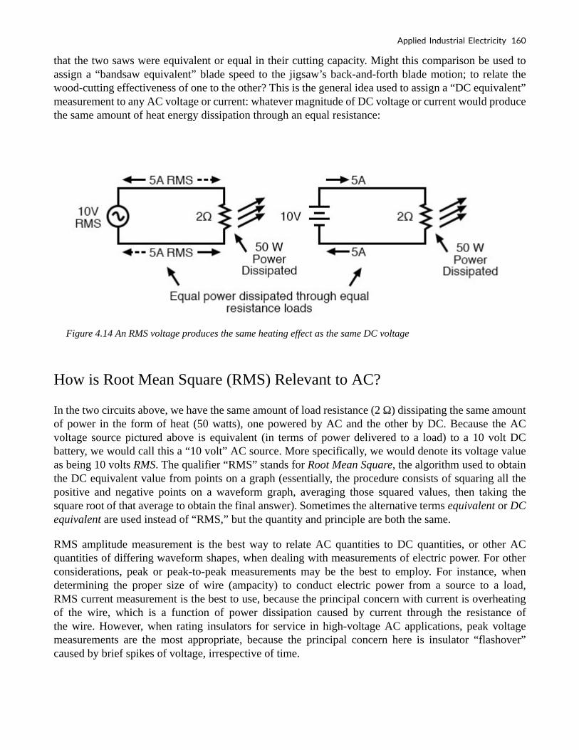
that the two saws were equivalent or equal in their cutting capacity. Might this comparison be used to assign a “bandsaw equivalent” blade speed to the jigsaw’s back-and-forth blade motion; to relate the wood-cutting effectiveness of one to the other? This is the general idea used to assign a “DC equivalent” measurement to any AC voltage or current: whatever magnitude of DC voltage or current would produce the same amount of heat energy dissipation through an equal resistance:
Figure 4.14 An RMS voltage produces the same heating effect as the same DC voltage
How is Root Mean Square (RMS) Relevant to AC?
In the two circuits above, we have the same amount of load resistance (2 Ω) dissipating the same amount of power in the form of heat (50 watts), one powered by AC and the other by DC. Because the AC voltage source pictured above is equivalent (in terms of power delivered to a load) to a 10 volt DC battery, we would call this a “10 volt” AC source. More specifically, we would denote its voltage value as being 10 volts RMS. The qualifier “RMS” stands for Root Mean Square, the algorithm used to obtain the DC equivalent value from points on a graph (essentially, the procedure consists of squaring all the positive and negative points on a waveform graph, averaging those squared values, then taking the square root of that average to obtain the final answer). Sometimes the alternative terms equivalent or DC equivalent are used instead of “RMS,” but the quantity and principle are both the same.
RMS amplitude measurement is the best way to relate AC quantities to DC quantities, or other AC quantities of differing waveform shapes, when dealing with measurements of electric power. For other considerations, peak or peak-to-peak measurements may be the best to employ. For instance, when determining the proper size of wire (ampacity) to conduct electric power from a source to a load, RMS current measurement is the best to use, because the principal concern with current is overheating of the wire, which is a function of power dissipation caused by current through the resistance of the wire. However, when rating insulators for service in high-voltage AC applications, peak voltage measurements are the most appropriate, because the principal concern here is insulator “flashover” caused by brief spikes of voltage, irrespective of time.
Applied Industrial Electricity 160

Instruments Used to Measure the Amplitude of a Waveform
Peak and peak-to-peak measurements are best performed with an oscilloscope, which can capture the crests of the waveform with a high degree of accuracy due to the fast action of the cathode-ray-tube in response to changes in voltage. For RMS measurements, analog meter movements (D’Arsonval, Weston, iron vane, electrodynamometer) will work so long as they have been calibrated in RMS figures. Because the mechanical inertia and dampening effects of an electromechanical meter movement makes the deflection of the needle naturally proportional to the average value of the AC, not the true RMS value, analog meters must be specifically calibrated (or mis-calibrated, depending on how you look at it) to indicate voltage or current in RMS units. The accuracy of this calibration depends on an assumed waveshape, usually a sine wave.
Electronic meters specifically designed for RMS measurement are best for the task. Some instrument manufacturers have designed ingenious methods for determining the RMS value of any waveform. One such manufacturer produces “True-RMS” meters with a tiny resistive heating element powered by a voltage proportional to that being measured. The heating effect of that resistance element is measured thermally to give a true RMS value with no mathematical calculations whatsoever, just the laws of physics in action in fulfillment of the definition of RMS. The accuracy of this type of RMS measurement is independent of waveshape.
Relationship of Peak, Peak-to-Peak, Average, and RMS
For “pure” waveforms, simple conversion coefficients exist for equating Peak, Peak-to-Peak, Average (practical, not algebraic), and RMS measurements to one another:
161 Tony R. Kuphaldt and John R. Haughery

Figure 4.15 Conversion factors for common waveforms.
In addition to RMS, average, peak (crest), and peak-to-peak measures of an AC waveform, there are ratios expressing the proportionality between some of these fundamental measurements. The crest factor of an AC waveform, for instance, is the ratio of its peak (crest) value divided by its RMS value. The form factor of an AC waveform is the ratio of its RMS value divided by its average value. Square-shaped waveforms always have crest and form factors equal to 1, since the peak is the same as the RMS and average values. Sinusoidal waveforms have an RMS value of 0.707 (the reciprocal of the square root of 2) and a form factor of 1.11 (0.707/0.636). Triangle- and sawtooth-shaped waveforms have RMS values of 0.577 (the reciprocal of square root of 3) and form factors of 1.15 (0.577/0.5).
Bear in mind that the conversion constants shown here for peak, RMS, and average amplitudes of sine waves, square waves, and triangle waves hold true only for pure forms of these waveshapes. The RMS and average values of distorted waveshapes are not related by the same ratios:
Figure 4.16 Arbitrary waveforms have no simple conversions.
Applied Industrial Electricity 162

This is a very important concept to understand when using an analog D’Arsonval meter movement to measure AC voltage or current. An analog D’Arsonval movement, calibrated to indicate sine-wave RMS amplitude, will only be accurate when measuring pure sine waves. If the waveform of the voltage or current being measured is anything but a pure sine wave, the indication given by the meter will not be the true RMS value of the waveform, because the degree of needle deflection in an analog D’Arsonval meter movement is proportional to the average value of the waveform, not the RMS. RMS meter calibration is obtained by “skewing” the span of the meter so that it displays a small multiple of the average value, which will be equal to be the RMS value for a particular waveshape and a particular waveshape only.
Since the sine-wave shape is most common in electrical measurements, it is the waveshape assumed for analog meter calibration, and the small multiple used in the calibration of the meter is 1.1107 (the form factor: 0.707/0.636: the ratio of RMS divided by average for a sinusoidal waveform). Any waveshape other than a pure sine wave will have a different ratio of RMS and average values, and thus a meter calibrated for sine-wave voltage or current will not indicate true RMS when reading a non-sinusoidal wave. Bear in mind that this limitation applies only to simple, analog AC meters not employing “True-RMS” technology.
Review
• The amplitude of an AC waveform is its height as depicted on a graph over time.
An amplitude measurement can take the form of peak, peak-to-peak, average, or
RMS quantity.
• Peak amplitude is the height of an AC waveform as measured from the zero mark to
the highest positive or lowest negative point on a graph. Also known as
the crest amplitude of a wave.
• Peak-to-peak amplitude is the total height of an AC waveform as measured from
maximum positive to maximum negative peaks on a graph. Often abbreviated as “P-
P”.
• Average amplitude is the mathematical “mean” of all a waveform’s points over the
period of one cycle. Technically, the average amplitude of any waveform with
equal-area portions above and below the “zero” line on a graph is zero. However, as
a practical measure of amplitude, a waveform’s average value is often calculated as
163 Tony R. Kuphaldt and John R. Haughery

the mathematical mean of all the points’ absolute values (taking all the negative
values and considering them as positive). For a sine wave, the average value so
calculated is approximately 0.637 of its peak value.
• “RMS” stands for Root Mean Square, and is a way of expressing an AC quantity of
voltage or current in terms functionally equivalent to DC. For example, 10 volts AC
RMS is the amount of voltage that would produce the same amount of heat
dissipation across a resistor of given value as a 10 volt DC power supply. Also
known as the “equivalent” or “DC equivalent” value of an AC voltage or current.
For a sine wave, the RMS value is approximately 0.707 of its peak value.
• The crest factor of an AC waveform is the ratio of its peak (crest) to its RMS value.
• The form factor of an AC waveform is the ratio of its RMS value to its average
value.
• Analog, electromechanical meter movements respond proportionally to
the average value of an AC voltage or current. When RMS indication is desired, the
meter’s calibration must be “skewed” accordingly. This means that the accuracy of
an electromechanical meter’s RMS indication is dependent on the purity of the
waveform: whether it is the exact same waveshape as the waveform used in
calibrating.
4.3 Single-phase Power Systems
Figure 4.17 Single phase power system schematic diagram shows little about the wiring of a practical power circuit.
Depicted above, is a very simple AC circuit. If the load resistor’s power dissipation were substantial, we might call this a “power circuit” or “power system” instead of regarding it as just a regular circuit.
Applied Industrial Electricity 164

The distinction between a “power circuit” and a “regular circuit” may seem arbitrary, but the practical concerns are definitely not.
Practical Circuit Analysis
One such concern is the size and cost of wiring necessary to deliver power from the AC source to the load. Normally, we do not give much thought to this type of concern if we’re merely analyzing a circuit for the sake of learning about the laws of electricity. However, in the real world, it can be a major concern. If we give the source in the above circuit a voltage value and also give power dissipation values to the two load resistors, we can determine the wiring needs for this particular circuit:
Examples 4.1
As a practical matter, the wiring for the 20 kW loads at 120 Vac is rather substantial (167 A).
165 Tony R. Kuphaldt and John R. Haughery
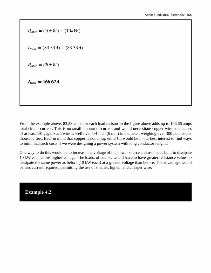
From the example above, 83.33 amps for each load resistor in the figure above adds up to 166.66 amps total circuit current. This is no small amount of current and would necessitate copper wire conductors of at least 1/0 gage. Such wire is well over 1/4 inch (6 mm) in diameter, weighing over 300 pounds per thousand feet. Bear in mind that copper is not cheap either! It would be in our best interest to find ways to minimize such costs if we were designing a power system with long conductor lengths.
One way to do this would be to increase the voltage of the power source and use loads built to dissipate 10 kW each at this higher voltage. The loads, of course, would have to have greater resistance values to dissipate the same power as before (10 kW each) at a greater voltage than before. The advantage would be less current required, permitting the use of smaller, lighter, and cheaper wire:
Example 4.2
Applied Industrial Electricity 166

Now our total circuit current is 83.33 amps, half of what it was before. We can now use number 4 gauge wire, which weighs less than half of what 1/0 gauge wire does per unit length. This is a considerable reduction in system cost with no degradation in performance. This is why power distribution system designers elect to transmit electric power using very high voltages (many thousands of volts): to capitalize on the savings realized by the use of smaller, lighter, cheaper wire.
167 Tony R. Kuphaldt and John R. Haughery

Dangers of Increasing the Source Voltage
However, this solution is not without disadvantages. Another practical concern with power circuits is the danger of electric shock from high voltages. Again, this is not usually the sort of thing we concentrate on while learning about the laws of electricity, but it is a very valid concern in the real world, especially when large amounts of power are being dealt with. The gain in efficiency realized by stepping up the circuit voltage presents us with an increased danger of electric shock. Power distribution companies tackle this problem by stringing their power lines along high poles or towers and insulating the lines from the supporting structures with large, porcelain insulators.
At the point of use (the electric power customer), there is still the issue of what voltage to use for powering loads. High voltage gives greater system efficiency by means of reduced conductor current, but it might not always be practical to keep power wiring out of reach at the point of use the way it can be elevated out of reach in distribution systems. This tradeoff between efficiency and danger is one that European power system designers have decided to risk, all their households and appliances operating at a nominal voltage of 240 volts instead of 120 volts as it is in North America. That is why tourists from America visiting Europe must carry small step-down transformers for their portable appliances, to step the 240 VAC (volts AC) power down to a more suitable 120 VAC.
Solutions for Voltage Delivery to Consumers
Step-down Transformers at End-point of Power use
Is there any way to realize the advantages of both increased efficiency and reduced safety hazard at the same time? One solution would be to install step-down transformers at the end-point of power use, just as the American tourist must do while in Europe. However, this would be expensive and inconvenient for anything but very small loads (where the transformers can be built cheaply) or very large loads (where the expense of thick copper wires would exceed the expense of a transformer).
Two Lower voltage Loads in Series
An alternative solution would be to use a higher voltage supply to provide power to two lower voltage loads in series. This approach combines the efficiency of a high-voltage system with the safety of a low-voltage system:
Applied Industrial Electricity 168

Figure 4.18 Series connected 120 Vac loads, driven by 240 Vac source at 83.3 A total current.
Notice the polarity markings (+ and -) for each voltage shown, as well as the unidirectional arrows for current. For the most part, I’ve avoided labeling “polarities” in the AC circuits we’ve been analyzing, even though the notation is valid to provide a frame of reference for phase. In later sections of this chapter, phase relationships will become very important, so I’m introducing this notation early on in the chapter for your familiarity.
The current through each load is the same as it was in the simple 120-volt circuit, but the currents are not additive because the loads are in series rather than parallel. The voltage across each load is only 120 volts, not 240, so the safety factor is better. Mind you, we still have a full 240 volts across the power system wires, but each load is operating at a reduced voltage. If anyone is going to get shocked, the odds are that it will be from coming into contact with the conductors of a particular load rather than from contact across the main wires of a power system.
Modifications to Two Load Series Design
There’s only one disadvantage to this design: the consequences of one load failing open, or being turned off (assuming each load has a series on/off switch to interrupt current) are not good. Being a series circuit, if either load were to open, the current would stop in the other load as well. For this reason, we need to modify the design a bit:
169 Tony R. Kuphaldt and John R. Haughery

Figure 4.19 Addition of neutral conductor allows loads to be individually driven.
Example 4.3
Applied Industrial Electricity 170

Split-phase Power System
Instead of a single 240-volt power supply, we use two 120 volt supplies (in phase with each other!) in series to produce 240 volts, then run a third wire to the connection point between the loads to handle the eventuality of one load opening. This is called a split-phase power system. Three smaller wires are still cheaper than the two wires needed with the simple parallel design, so we’re still ahead on efficiency. The astute observer will note that the neutral wire only has to carry the difference of current between the two loads back to the source. In the above case, with perfectly “balanced” loads consuming equal amounts of power, the neutral wire carries zero current.
Notice how the neutral wire is connected to earth ground at the power supply end. This is a common feature in power systems containing “neutral” wires, since grounding the neutral wire ensures the least possible voltage at any given time between any “hot” wire and earth ground.
An essential component of a split-phase power system is the dual AC voltage source. Fortunately, designing and building one is not difficult. Since most AC systems receive their power from a step-down transformer anyway (stepping voltage down from high distribution levels to a user-level voltage like 120 or 240), that transformer can be built with a center-tapped secondary winding:
Figure 4.20 American 120/240 Vac power is derived from a center tapped utility transformer.
If the AC power comes directly from a generator (alternator), the coils can be similarly center-tapped for the same effect. The extra expense to include a center-tap connection in a transformer or alternator winding is minimal.
Here is where the (+) and (-) polarity markings really become important. This notation is often used to reference the phasings of multiple AC voltage sources, so it is clear whether they are aiding (“boosting”) each other or opposing (“bucking”) each other. If not for these polarity markings, phase relations between multiple AC sources might be very confusing. Note that the split-phase sources in the schematic (each one 120 volts ∠ 0°), with polarity marks (+) to (-) just like series-aiding batteries can alternatively be represented as such:
171 Tony R. Kuphaldt and John R. Haughery

Figure 4.21 Split phase 120/240 Vac source is equivalent to two series aiding 120 Vac sources.
Example 4.4
To mathematically calculate voltage between “hot” wires, we must subtract voltages, because
their polarity marks show them to be opposed to each other:
Polar
Rectangular
If we mark the two sources’ common connection point (the neutral wire) with the same polarity mark (-), we must express their relative phase shifts as being 180° apart. Otherwise, we’d be denoting two voltage sources in direct opposition with each other, which would give 0 volts between the two “hot” conductors. Why am I taking the time to elaborate on polarity marks and phase angles? It will make more sense in the next section!
Power systems in American households and light industry are most often of the split-phase variety,
Applied Industrial Electricity 172

providing so-called 120/240 VAC power. The term “split-phase” merely refers to the split-voltage supply in such a system. In a more general sense, this kind of AC power supply is called single phase because both voltage waveforms are in phase, or in step, with each other.
The term “single phase” is a counterpoint to another kind of power system called “polyphase” which we are about to investigate in detail. Apologies for the long introduction leading up to the title-topic of this chapter. The advantages of polyphase power systems are more obvious if one first has a good understanding of single-phase systems.
Review
• Single phase power systems are defined by having an AC source with only one
voltage waveform.
• A split-phase power system is one with multiple (in-phase) AC voltage sources
connected in series, delivering power to loads at more than one voltage, with more
than two wires. They are used primarily to achieve a balance between system
efficiency (low conductor currents) and safety (low load voltages).
• Split-phase AC sources can be easily created by center-tapping the coil windings of
transformers or alternators.
4.4 AC phase
AC phase
Things start to get complicated when we need to relate two or more AC voltages or currents that are out of step with each other. By “out of step,” I mean that the two waveforms are not synchronized: that their peaks and zero points do not match up at the same points in time. The graph in figure below illustrates an example of this.
173 Tony R. Kuphaldt and John R. Haughery

Figure 4.22 Out of phase wave forms
The two waves shown above (A versus B) are of the same amplitude and frequency, but they are out of step with each other. In technical terms, this is called a phase shift. Earlier we saw how we could plot a “sine wave” by calculating the trigonometric sine function for angles ranging from 0 to 360 degrees, a full circle. The starting point of a sine wave was zero amplitude at zero degrees, progressing to full positive amplitude at 90 degrees, zero at 180 degrees, full negative at 270 degrees, and back to the starting point of zero at 360 degrees. We can use this angle scale along the horizontal axis of our waveform plot to express how far out of step one wave is with another:
Figure 4.23 Wave A leads wave B by 45°
The shift between these two waveforms is about 45 degrees, the “A” wave being ahead of the “B” wave. A sampling of different phase shifts is given in the following graphs to better illustrate this concept:
Applied Industrial Electricity 174

Figure 4.24 Examples of phase shifts.
Because the waveforms in the above examples are at the same frequency, they will be out of step by the same angular amount at every point in time. For this reason, we can express phase shift for two or more waveforms of the same frequency as a constant quantity for the entire wave, and not just an expression of shift between any two particular points along the waves. That is, it is safe to say something like, “voltage ‘A’ is 45 degrees out of phase with voltage ‘B’.” Whichever waveform is ahead in its evolution is said to be leading and the one behind is said to be lagging. Phase shift, like voltage, is always a measurement relative between two things. There’s really no such thing as a waveform with an absolute phase measurement because there’s no known universal reference for phase. Typically in the analysis of AC circuits, the voltage waveform of the power supply is used as a reference for phase, that voltage stated as “xxx volts at 0 degrees.” Any other AC voltage or current in that circuit will have its phase shift expressed in terms relative to that source voltage. This is what makes AC circuit calculations more complicated than DC. When applying Ohm’s Law and Kirchhoff’s Laws, quantities of AC voltage and current must reflect phase shift as well as amplitude. Mathematical operations of addition, subtraction, multiplication, and division must operate on these quantities of phase shift as well as amplitude. Fortunately, there is a mathematical system of quantities called complex numbers ideally suited for this task of representing amplitude and phase. Because the subject of complex numbers is so essential to the understanding of AC circuits, the next chapter will be devoted to that subject alone.
175 Tony R. Kuphaldt and John R. Haughery
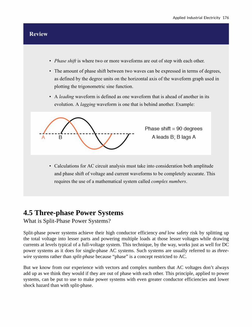
Review
• Phase shift is where two or more waveforms are out of step with each other.
• The amount of phase shift between two waves can be expressed in terms of degrees,
as defined by the degree units on the horizontal axis of the waveform graph used in
plotting the trigonometric sine function.
• A leading waveform is defined as one waveform that is ahead of another in its
evolution. A lagging waveform is one that is behind another. Example:
• Calculations for AC circuit analysis must take into consideration both amplitude
and phase shift of voltage and current waveforms to be completely accurate. This
requires the use of a mathematical system called complex numbers.
4.5 Three-phase Power Systems What is Split-Phase Power Systems?
Split-phase power systems achieve their high conductor efficiency and low safety risk by splitting up the total voltage into lesser parts and powering multiple loads at those lesser voltages while drawing currents at levels typical of a full-voltage system. This technique, by the way, works just as well for DC power systems as it does for single-phase AC systems. Such systems are usually referred to as three-wire systems rather than split-phase because “phase” is a concept restricted to AC.
But we know from our experience with vectors and complex numbers that AC voltages don’t always add up as we think they would if they are out of phase with each other. This principle, applied to power systems, can be put to use to make power systems with even greater conductor efficiencies and lower shock hazard than with split-phase.
Applied Industrial Electricity 176

Example 4.5
Two 120° Out of Phase Voltage Sources
Suppose that we had two sources of AC voltage connected in series just like the split-phase
system we saw before, except that each voltage source was 120° out of phase with the other:
(Figure below)
Pair of 120 Vac sources phased 120°, similar to split-phase.
Since each voltage source is 120 volts, and each load resistor is connected directly in parallel
with its respective source, the voltage across each load must be 120 volts as well. Given load
currents of 83.33 amps, each load must still be dissipating 10 kilowatts of power. However,
voltage between the two “hot” wires is not 240 volts (120 ∠ 0° – 120 ∠ 180°) because the
phase difference between the two sources is not 180°. Instead, the voltage is:
Nominally, we say that the voltage between “hot” conductors is 208 volts (rounding up), and
thus the power system voltage is designated as 120/208 V.
177 Tony R. Kuphaldt and John R. Haughery

Example 4.6
If we calculate the current through the “neutral” conductor, we find that it is not zero, even
with balanced load resistances. Kirchhoff’s Current Law tells us that the currents entering and
exiting the node between the two loads must be zero:
So, we find that the “neutral” wire is carrying a full 83.33 amps, just like each “hot” wire.
Note that we are still conveying 20 kW of total power to the two loads, with each load’s “hot” wire carrying 83.33 amps as before. With the same amount of current through each “hot” wire, we must use the same gauge copper conductors, so we haven’t reduced system cost over the split-phase 120/240
Applied Industrial Electricity 178

system. However, we have realized a gain in safety, because the overall voltage between the two “hot” conductors is 32 volts lower than it was in the split-phase system (208 volts instead of 240 volts).
Three 120° Out of Phase Voltage Sources
The fact that the neutral wire is carrying 83.33 amps of current raises an interesting possibility: since its carrying current anyway, why not use that third wire as another “hot” conductor, powering another load resistor with a third 120 volt source having a phase angle of 240°? That way, we could transmit more power (another 10 kW) without having to add any more conductors. Let’s see how this might look:
Figure 4.25 With a third load phased 120° to the other two, the currents are the same as for two loads.
Polyphase Circuit
This circuit we’ve been analyzing with three voltage sources is called a polyphase circuit. The prefix “poly” simply means “more than one,” as in “polytheism” (belief in more than one deity), “polygon” (a geometrical shape made of multiple line segments: for example, pentagon and hexagon), and “polyatomic” (a substance composed of multiple types of atoms). Since the voltage sources are all at different phase angles (in this case, three different phase angles), this is a “polyphase” circuit. More specifically, it is a three-phase circuit, the kind used predominantly in large power distribution systems.
Single-Phase System
Let’s survey the advantages of a three-phase power system over a single-phase system of equivalent load voltage and power capacity. A single-phase system with three loads connected directly in parallel would have a very high total current (83.33 times 3, or 250 amps.
179 Tony R. Kuphaldt and John R. Haughery

Figure 4.26 For comparison, three 10 Kw loads on a 120 Vac system draw 250 A.
This would necessitate 3/0 gage copper wire (very large!), at about 510 pounds per thousand feet, and with a considerable price tag attached. If the distance from source to load was 1000 feet, we would need over a half-ton of copper wire to do the job.
Split-phase System
On the other hand, we could build a split-phase system with two 15 kW, 120 volt loads.
Figure 4.27 Split phase system draws half the current of 125 A at 240 Vac compared to 120 Vac system.
Our current is half of what it was with the simple parallel circuit, which is a great improvement. We could get away with using number 2 gauge copper wire at a total mass of about 600 pounds, figuring about 200 pounds per thousand feet with three runs of 1000 feet each between source and loads. However, we also have to consider the increased safety hazard of having 240 volts present in the system, even though each load only receives 120 volts. Overall, there is greater potential for a dangerous electric shock to occur.
Applied Industrial Electricity 180

Three-Phase System
When we contrast these two examples against our three-phase system (Figure above), the advantages are quite clear. First, the conductor currents are quite a bit less (83.33 amps versus 125 or 250 amps), permitting the use of much thinner and lighter wire. We can use number 4 gauge wire at about 125 pounds per thousand feet, which will total 500 pounds (four runs of 1000 feet each) for our example circuit. This represents significant cost savings over the split-phase system, with the additional benefit that the maximum voltage in the system is lower (208 versus 240).
One question remains to be answered: how in the world do we get three AC voltage sources whose phase angles are exactly 120° apart? Obviously we can’t center-tap a transformer or alternator winding like we did in the split-phase system, since that can only give us voltage waveforms that are either in phase or 180° out of phase. Perhaps we could figure out some way to use capacitors and inductors to create phase shifts of 120°, but then those phase shifts would depend on the phase angles of our load impedances as well (substituting a capacitive or inductive load for a resistive load would change everything!).
The best way to get the phase shifts we’re looking for is to generate it at the source: construct the AC generator (alternator) providing the power in such a way that the rotating magnetic field passes by three sets of wire windings, each set spaced 120o apart around the circumference of the machine as in the figure below.
Figure 4.28 (a) Single-phase alternator, (b) Three-phase alternator.
Together, the six “pole” windings of a three-phase alternator are connected to comprise three winding pairs, each pair producing AC voltage with a phase angle 120° shifted from either of the other two winding pairs. The interconnections between pairs of windings (as shown for the single-phase alternator: the jumper wire between windings 1a and 1b) have been omitted from the three-phase alternator drawing for simplicity.
In our example circuit, we showed the three voltage sources connected together in a “Y” configuration (sometimes called the “star” configuration), with one lead of each source tied to a common point (the node where we attached the “neutral” conductor). The common way to depict this connection scheme is to draw the windings in the shape of a “Y” like the figure below.
181 Tony R. Kuphaldt and John R. Haughery

Figure 4.29 Alternator “Y” configuration.
The “Y” configuration is not the only option open to us, but it is probably the easiest to understand at first. More to come on this subject later in the chapter.
Review
• A single-phase power system is one where there is only one AC voltage source (one
source voltage waveform).
• A split-phase power system is one where there are two voltage sources, 180° phase-
shifted from each other, powering a two series-connected loads. The advantage of
this is the ability to have lower conductor currents while maintaining low load
voltages for safety reasons.
• A polyphase power system uses multiple voltage sources at different phase angles
from each other (many “phases” of voltage waveforms at work). A polyphase power
system can deliver more power at less voltage with smaller-gage conductors than
single- or split-phase systems.
• The phase-shifted voltage sources necessary for a polyphase power system are
created in alternators with multiple sets of wire windings. These winding sets are
Applied Industrial Electricity 182

spaced around the circumference of the rotor’s rotation at the desired angle(s).
4.6 Phase Rotation
Three-Phase Alternator
Let’s take the three-phase alternator design laid out earlier and watch what happens as the magnet rotates.
Figure 4.30 Three-phase alternator
The phase angle shift of 120° is a function of the actual rotational angle shift of the three pairs of windings. If the magnet is rotating clockwise, winding 3 will generate its peak instantaneous voltage exactly 120° (of alternator shaft rotation) after winding 2, which will hit its peak 120° after winding 1. The magnet passes by each pole pair at different positions in the rotational movement of the shaft. Where we decide to place the windings will dictate the amount of phase shift between the windings’ AC voltage waveforms. If we make winding 1 our “reference” voltage source for phase angle (0°), then winding 2
183 Tony R. Kuphaldt and John R. Haughery

will have a phase angle of -120° (120° lagging, or 240° leading) and winding 3 an angle of -240° (or 120° leading).
Phase Sequence
This sequence of phase shifts has a definite order. For clockwise rotation of the shaft, the order is 1-2-3 (winding 1 peak first, them winding 2, then winding 3). This order keeps repeating itself as long as we continue to rotate the alternator’s shaft.
Figure 4.31 Clockwise rotation phase sequence: 1-2-3.
However, if we reverse the rotation of the alternator’s shaft (turn it counter-clockwise), the magnet will pass by the pole pairs in the opposite sequence. Instead of 1-2-3, we’ll have 3-2-1. Now, winding 2’s waveform will be leading 120° ahead of 1 instead of lagging, and 3 will be another 120° ahead of 2.
Figure 4.32 Counterclockwise rotation phase sequence: 3-2-1.
Applied Industrial Electricity 184
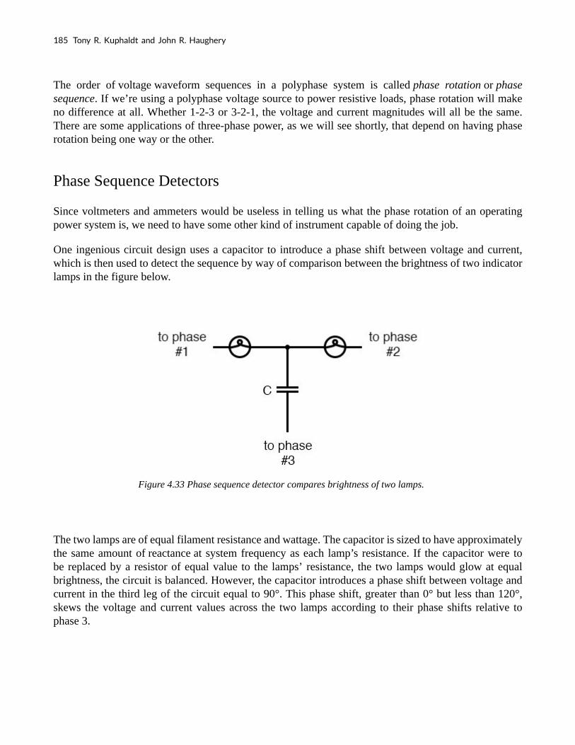
The order of voltage waveform sequences in a polyphase system is called phase rotation or phase sequence. If we’re using a polyphase voltage source to power resistive loads, phase rotation will make no difference at all. Whether 1-2-3 or 3-2-1, the voltage and current magnitudes will all be the same. There are some applications of three-phase power, as we will see shortly, that depend on having phase rotation being one way or the other.
Phase Sequence Detectors
Since voltmeters and ammeters would be useless in telling us what the phase rotation of an operating power system is, we need to have some other kind of instrument capable of doing the job.
One ingenious circuit design uses a capacitor to introduce a phase shift between voltage and current, which is then used to detect the sequence by way of comparison between the brightness of two indicator lamps in the figure below.
Figure 4.33 Phase sequence detector compares brightness of two lamps.
The two lamps are of equal filament resistance and wattage. The capacitor is sized to have approximately the same amount of reactance at system frequency as each lamp’s resistance. If the capacitor were to be replaced by a resistor of equal value to the lamps’ resistance, the two lamps would glow at equal brightness, the circuit is balanced. However, the capacitor introduces a phase shift between voltage and current in the third leg of the circuit equal to 90°. This phase shift, greater than 0° but less than 120°, skews the voltage and current values across the two lamps according to their phase shifts relative to phase 3.
185 Tony R. Kuphaldt and John R. Haughery

Exchanging Hot Wires
There is a much easier way to reverse phase sequence than reversing alternator rotation: just exchange any two of the three “hot” wires going to a three-phase load.
This trick makes more sense if we take another look at a running phase sequence of a three-phase voltage source:
1-2-3 rotation: 1-2-3-1-2-3-1-2-3-1-2-3-1-2-3 . . .
3-2-1 rotation: 3-2-1-3-2-1-3-2-1-3-2-1-3-2-1 . . .
What is commonly designated as a “1-2-3” phase rotation could just as well be called “2-3-1” or “3-1-2,” going from left to right in the number string above? Likewise, the opposite rotation (3-2-1) could just as easily be called “2-1-3” or “1-3-2.”
Starting out with a phase rotation of 3-2-1, we can try all the possibilities for swapping any two of the wires at a time and see what happens to the resulting sequence in the figure below.
Figure 4.34 All possibilities of swapping any two wires.
No matter which pair of “hot” wires out of the three we choose to swap, the phase rotation ends up being reversed (1-2-3 gets changed to 2-1-3, 1-3-2 or 3-2-1, all equivalent).
Applied Industrial Electricity 186

Review
• Phase rotation, or phase sequence, is the order in which the voltage waveforms of a
polyphase AC source reach their respective peaks. For a three-phase system, there
are only two possible phase sequences: 1-2-3 and 3-2-1, corresponding to the two
possible directions of alternator rotation.
• Phase rotation has no impact on resistive loads, but it will have an impact on
unbalanced reactive loads, as shown in the operation of a phase rotation detector
circuit.
• Phase rotation can be reversed by swapping any two of the three “hot” leads
supplying three-phase power to a three-phase load.
4.7 Three-phase Y and Delta Configurations
Three-phase Wye(Y) Connection
Initially, we explored the idea of three-phase power systems by connecting three voltage sources together in what is commonly known as the “Y” (or “star”) configuration. This configuration of voltage sources is characterized by a common connection point joining one side of each source.
187 Tony R. Kuphaldt and John R. Haughery

Figure 4.35 Three-phase “Y” connection has three voltage sources connected to a common point.
If we draw a circuit showing each voltage source to be a coil of wire (alternator or transformer winding) and do some slight rearranging, the “Y” configuration becomes more obvious in the figure below.
Figure 4.36 Three-phase, four-wire “Y” connection uses a “common” fourth wire.
The three conductors leading away from the voltage sources (windings) toward a load are typically called lines, while the windings themselves are typically called phases. In a Y-connected system, there may or may not (Figure below) be a neutral wire attached at the junction point in the middle, although it certainly helps alleviate potential problems should one element of a three-phase load fail open, as discussed earlier.
Applied Industrial Electricity 188

Figure 4.37 Three-phase, three-wire “Y” connection does not use the neutral wire.
Voltage and Current Values in Three-Phase Systems
When we measure voltage and current in three-phase systems, we need to be specific as to where we’re measuring. Line voltage refers to the amount of voltage measured between any two line conductors in a balanced three-phase system. With the above circuit, the line voltage is roughly 208 volts. Phase voltage refers to the voltage measured across any one component (source winding or load impedance) in a balanced three-phase source or load. For the circuit shown above, the phase voltage is 120 volts. The terms line current and phase current follows the same logic: the former referring to the current through any one line conductor, and the latter to the current through any one component.
Y-connected sources and loads always have line voltages greater than phase voltages, and line currents equal to phase currents. If the Y-connected source or load is balanced, the line voltage will be equal to the phase voltage times the square root of 3:
For “Y” circuits:
189 Tony R. Kuphaldt and John R. Haughery
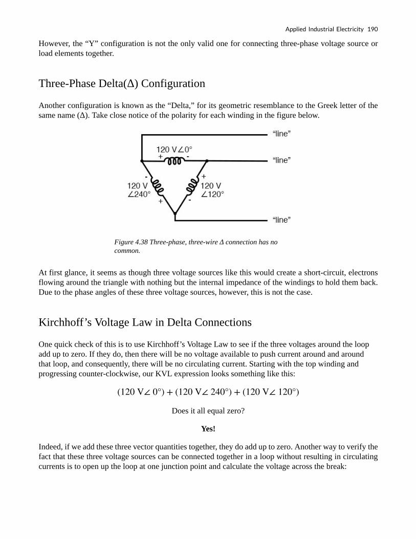
However, the “Y” configuration is not the only valid one for connecting three-phase voltage source or load elements together.
Three-Phase Delta(Δ) Configuration
Another configuration is known as the “Delta,” for its geometric resemblance to the Greek letter of the same name (Δ). Take close notice of the polarity for each winding in the figure below.
Figure 4.38 Three-phase, three-wire Δ connection has no common.
At first glance, it seems as though three voltage sources like this would create a short-circuit, electrons flowing around the triangle with nothing but the internal impedance of the windings to hold them back. Due to the phase angles of these three voltage sources, however, this is not the case.
Kirchhoff’s Voltage Law in Delta Connections
One quick check of this is to use Kirchhoff’s Voltage Law to see if the three voltages around the loop add up to zero. If they do, then there will be no voltage available to push current around and around that loop, and consequently, there will be no circulating current. Starting with the top winding and progressing counter-clockwise, our KVL expression looks something like this:
Does it all equal zero?
Yes!
Indeed, if we add these three vector quantities together, they do add up to zero. Another way to verify the fact that these three voltage sources can be connected together in a loop without resulting in circulating currents is to open up the loop at one junction point and calculate the voltage across the break:
Applied Industrial Electricity 190

Figure 4.39 Voltage across open Δ should be zero.
Starting with the right winding (120 V ∠ 120°) and progressing counter-clockwise, our KVL equation looks like this:
Sure enough, there will be zero voltage across the break, telling us that no current will circulate within the triangular loop of windings when that connection is made complete.
Having established that a Δ-connected three-phase voltage source will not burn itself to a crisp due to circulating currents, we turn to its practical use as a source of power in three-phase circuits. Because each pair of line conductors is connected directly across a single winding in a Δ circuit, the line voltage will be equal to the phase voltage. Conversely, because each line conductor attaches at a node between two windings, the line current will be the vector sum of the two joining phase currents. Not surprisingly, the resulting equations for a Δ configuration are as follows:
191 Tony R. Kuphaldt and John R. Haughery

For Δ (“Delta”) circuits:
Example 4.7
Delta Connection Example Circuit Analysis
Let’s see how this works in an example circuit: (Figure below)
With each load resistance receiving 120 volts from its respective phase winding at the source,
the current in each phase of this circuit will be 83.33 amps:
Applied Industrial Electricity 192

Advantages of the Delta Three-Phase System
So each line current in this three-phase power system is equal to 144.34 amps, which is substantially more than the line currents in the Y-connected system we looked at earlier. One might wonder if we’ve lost all the advantages of three-phase power here, given the fact that we have such greater conductor currents, necessitating thicker, more costly wire. The answer is no. Although this circuit would require three number 1 gauge copper conductors (at 1000 feet of distance between source and load this equates to a little over 750 pounds of copper for the whole system), it is still less than the 1000+ pounds of copper required for a single-phase system delivering the same power (30 kW) at the same voltage (120 volts conductor-to-conductor).
One distinct advantage of a Δ-connected system is its lack of a neutral wire. With a Y-connected system, a neutral wire was needed in case one of the phase loads were to fail open (or be turned off), in order to keep the phase voltages at the load from changing. This is not necessary (or even possible!) in a Δ-connected circuit. With each load phase element directly connected across a respective source phase winding, the phase voltage will be constant regardless of open failures in the load elements.
Perhaps the greatest advantage of the Δ-connected source is its fault tolerance. It is possible for one of the windings in a Δ-connected three-phase source to fail open (Figure below) without affecting load voltage or current!
193 Tony R. Kuphaldt and John R. Haughery
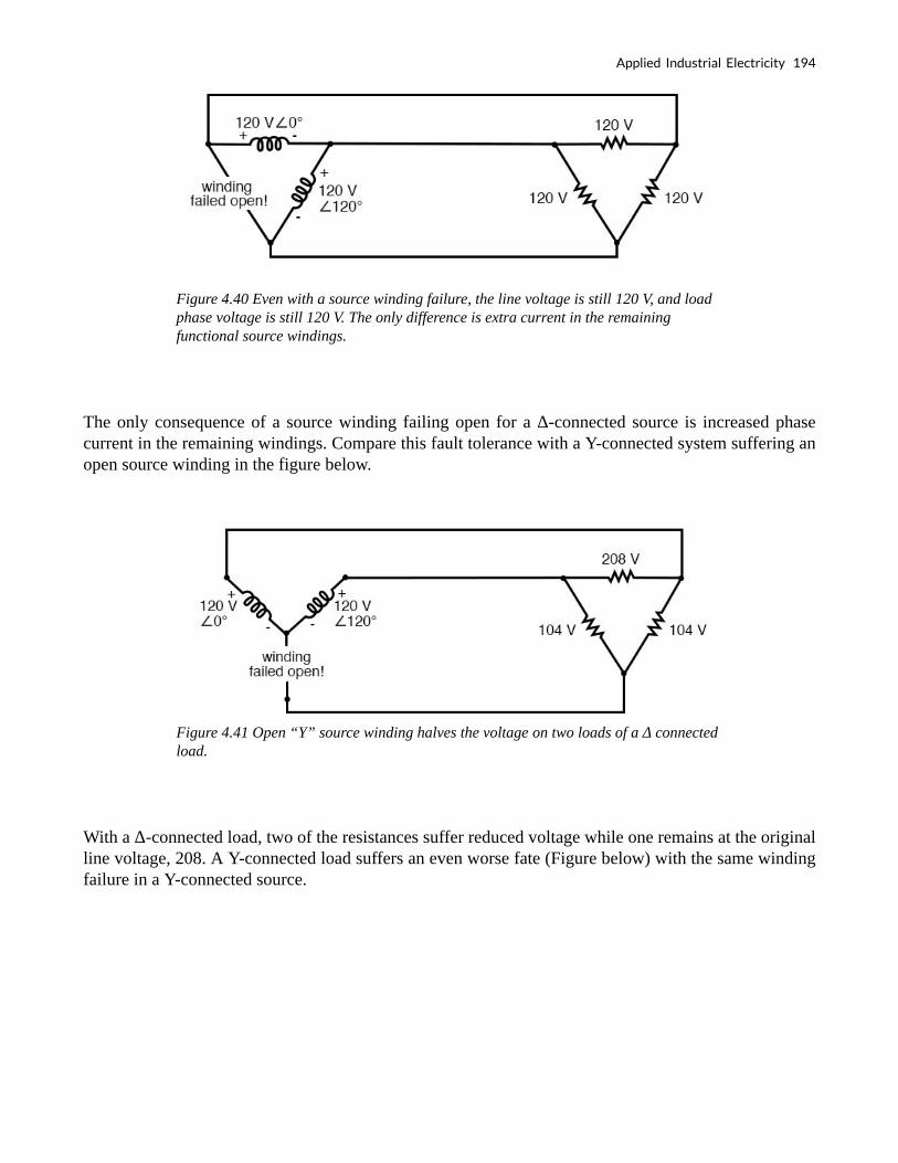
Figure 4.40 Even with a source winding failure, the line voltage is still 120 V, and load phase voltage is still 120 V. The only difference is extra current in the remaining functional source windings.
The only consequence of a source winding failing open for a Δ-connected source is increased phase current in the remaining windings. Compare this fault tolerance with a Y-connected system suffering an open source winding in the figure below.
Figure 4.41 Open “Y” source winding halves the voltage on two loads of a Δ connected load.
With a Δ-connected load, two of the resistances suffer reduced voltage while one remains at the original line voltage, 208. A Y-connected load suffers an even worse fate (Figure below) with the same winding failure in a Y-connected source.
Applied Industrial Electricity 194

Figure 4.42 Open source winding of a “Y-Y” system halves the voltage on two loads, and loses one load entirely.
In this case, two load resistances suffer reduced voltage while the third loses supply voltage completely! For this reason, Δ-connected sources are preferred for reliability. However, if dual voltages are needed (e.g. 120/208) or preferred for lower line currents, Y-connected systems are the configuration of choice.
Review
• The conductors connected to the three points of a three-phase source or load are
called lines.
• The three components comprising a three-phase source or load are called phases.
• Line voltage is the voltage measured between any two lines in a three-phase circuit.
• Phase voltage is the voltage measured across a single component in a three-phase
source or load.
• Line current is the current through any one line between a three-phase source and
load.
• Phase current is the current through any one component comprising a three-phase
source or load.
• In balanced “Y” circuits, the line voltage is equal to phase voltage times the square
root of 3, while the line current is equal to phase current.
195 Tony R. Kuphaldt and John R. Haughery

• For “Y” circuits:
• In balanced Δ circuits, the line voltage is equal to phase voltage, while the line
current is equal to phase current times the square root of 3.
• For Δ (“Delta”) circuits:
• Δ-connected three-phase voltage sources give greater reliability in the event of
winding failure than Y-connected sources. However, Y-connected sources can
deliver the same amount of power with less line current than Δ-connected sources.
Applied Industrial Electricity 196

5. MOTOR CHARACTERISTICS
5.1 Introduction
After the introduction of the DC electrical distribution system by Edison in the United States, a gradual transition to the more economical AC system commenced. The lighting worked as well on AC as on DC. Transmission of electrical energy covered longer distances at a lower loss with alternating current. However, motors were a problem with alternating current. Initially, AC motors were constructed like DC motors, but numerous problems were encountered due to changing magnetic fields.
Figure 5.1 AC electric motor family diagram
Charles P. Steinmetz contributed to solving these problems with his investigation of hysteresis losses in iron armatures. Nikola Tesla envisioned an entirely new type of motor when he visualized a spinning turbine, not spun by water or steam, but by a rotating magnetic field. His new type of motor, the AC induction motor, is the workhorse of the industry to this day. Its ruggedness and simplicity make for long life, high reliability, and low maintenance. Yet small brushed AC motors, similar to the DC variety, persist in small appliances along with small Tesla induction motors. Above one horsepower (750 W), the Tesla motor reigns supreme.
Modern solid-state electronic circuits drive brushless DC motors with AC waveforms generated from a DC source. The brushless DC motor, actually an AC motor, is replacing the conventional brushed
197

DC motor in many applications. And, the stepper motor, a digital version of the motor, is driven by alternating current square waves, again, generated by solid-state circuitry. The figure above shows the family tree of the AC motors described in this chapter.
Cruise ships and other large vessels replace reduction geared driveshafts with large multi-megawatt generators and motors. Such has been the case with diesel-electric locomotives on a smaller scale for many years.
Figure 5.2 Motor system level diagram
At the system level, (Figure above) a motor takes in electrical energy in terms of a potential difference and a current flow, converting it to mechanical work. Unfortunately, electric motors are not 100% efficient. Some of the electric energy is lost to heat, another form of energy, due to I2R losses (also called copper losses) in the motor windings. The heat is an undesired byproduct of this conversion. It must be removed from the motor and may adversely affect longevity. Thus, one goal is to maximize motor efficiency, reducing heat loss. AC motors also have some losses not encountered by DC motors: hysteresis and eddy currents.
5.2 Tesla Polyphase Induction Motors
Most AC motors are induction motors. Induction motors are favored due to their ruggedness and simplicity. In fact, 90% of industrial motors are induction motors.
Nikola Tesla conceived the basic principles of the polyphase induction motor in 1883 and had a half horsepower (400 watts) model by 1888. Tesla sold the manufacturing rights to George Westinghouse for $65,000.Most large ( > 1 hp or 1 kW) industrial motors are polyphase induction motors. By polyphase, we mean that the stator contains multiple distinct windings per motor pole, driven by corresponding time-shifted sine waves. In practice, this is two or three phases. Large industrial motors are 3-phase. While we include numerous illustrations of two-phase motors for simplicity, we must emphasize that nearly all polyphase motors are three-phase. By induction motor, we mean that the stator windings induce a current flow in the rotor conductors, like a transformer, unlike a brushed DC commutator motor.
Applied Industrial Electricity 198

AC Induction Motor Construction
An induction motor is composed of a rotor, known as an armature, and a stator containing windings connected to a polyphase energy source as shown in the figure below. The simple 2-phase induction motor below is similar to the 1/2 horsepower motor which Nikola Tesla introduced in 1888.
Figure 5.3 Tesla polyphase induction motor
The stator in the figure above is wound with pairs of coils corresponding to the phases of electrical energy available. The 2-phase induction motor stator above has 2-pairs of coils, one pair for each of the two phases of AC. The individual coils of a pair are connected in series and correspond to the opposite poles of an electromagnet. That is, one coil corresponds to an N-pole, the other to an S-pole until the phase of AC changes polarity. The other pair of coils is oriented 90° in space to the first pair. This pair of coils is connected to AC shifted in time by 90° in the case of a 2-phase motor. In Tesla’s time, the source of the two phases of AC was a 2-phase alternator. The stator in the figure above has salient, obvious protruding poles, as used on Tesla’s early induction motor. This design is used to this day for sub-fractional horsepower motors (<50 watts). However, for larger motors, less torque pulsation and higher efficiency results if the coils are embedded into slots cut into the stator laminations (figure below).
199 Tony R. Kuphaldt and John R. Haughery

Figure 5.4 Stator frame showing slots for windings
The stator laminations are thin insulated rings with slots punched from sheets of electrical grade steel. A stack of these is secured by end screws, which may also hold the end housings.
Figure 5.5 Stator with (a) 2-φ and (b) 3-φ windings
In the figure above, the windings for both a two-phase motor and a three-phase motor have been installed in the stator slots. The coils are wound on an external fixture, then worked into the slots. Insulation wedged between the coil periphery and the slot protects against abrasion.Actual stator windings are more complex than the single windings per pole in the figure above. Comparing the 2-φ motor to
Applied Industrial Electricity 200

Tesla’s 2-φ motor with salient poles, the number of coils is the same. In actual large motors, a pole winding is divided into identical coils inserted into many smaller slots than above. This group is called a phase belt (see the figure below). The distributed coils of the phase belt cancel some of the odd harmonics, producing a more sinusoidal magnetic field distribution across the pole. This is shown in the synchronous motor section. The slots at the edge of the pole may have fewer turns than the other slots. Edge slots may contain windings from two phases. That is, the phase belts overlap.
Figure 5.6 Phase belts overlap
The key to the popularity of the AC induction motor is its simplicity as evidenced by the simple rotor (figure below). The rotor consists of a shaft, a steel laminated rotor, and an embedded copper or aluminum squirrel cage, shown at (b) removed from the rotor. As compared to a DC motor armature, there is no commutator. This eliminates the brushes, arcing, sparking, graphite dust, brush adjustment and replacement, and re-machining of the commutator.
Figure 5.7 Laminated rotor with (a) embedded squirrel cage, (b) conductive cage removed from the rotor
201 Tony R. Kuphaldt and John R. Haughery

The squirrel cage conductors may be skewed, twisted, with respect to the shaft. The misalignment with the stator slots reduces torque pulsations.Both rotor and stator cores are composed of a stack of insulated laminations. The laminations are coated with insulating oxide or varnish to minimize eddy current losses. The alloy used in the laminations is selected for low hysteresis losses.
Theory of Operation of Induction Motors
A short explanation of operation is that the stator creates a rotating magnetic field which drags the rotor around.The theory of operation of induction motors is based on a rotating magnetic field. One way of creating a rotating magnetic field is to rotate a permanent magnet. If the moving magnetic lines of flux cut a conductive disk, it will follow the motion of the magnet. The lines of flux cutting the conductor will induce a voltage, and consequent current flow, in the conductive disk. This current flow creates an electromagnet whose polarity opposes the motion of the permanent magnet– Lenz’s Law. The polarity of the electromagnet is such that it pulls against the permanent magnet. The disk follows with a little less speed than the permanent magnet.
Figure 5.8 Rotating magnetic field produces torque in conductive disk
Rotating magnetic field produces torque in conductive disk
The torque developed by the disk is proportional to the number of flux lines cutting the disk and the rate at which it cuts the disk. If the disk were to spin at the same rate as the permanent magnet, there would be no flux cutting the disk, no induced current flow, no electromagnet field, no torque. Thus, the disk speed will always fall behind that of the rotating permanent magnet, so that lines of flux cut the disk induce a current, create an electromagnetic field in the disk, which follows the permanent magnet. If a load is
Applied Industrial Electricity 202

applied to the disk, slowing it, more torque will be developed as more lines of flux cut the disk. Torque is proportional to slip, the degree to which the disk falls behind the rotating magnet. More slip corresponds to more flux cutting the conductive disk, developing more torque.An analog automotive eddy-current speedometer is based on the principle illustrated above. With the disk restrained by a spring, disk and needle deflection is proportional to the magnet rotation rate.A rotating magnetic field is created by two coils placed at right angles to each other, driven by currents which are 90° out of phase. This should not be surprising if you are familiar with oscilloscope Lissajous patterns.
Figure 5.9 Out of phase (90°), sine waves produce circular Lissajous pattern
Out of phase (90°), sine waves produce circular Lissajous patternIn the figure above, a circular Lissajous is produced by driving the horizontal and vertical oscilloscope inputs with 90° out of phase sine waves. Starting at (a) with maximum “X” and minimum “Y” deflection, the trace moves up and left toward (b). Between (a) and (b) the two waveforms are equal to 0.707 Vpk at 45°. This point (0.707, 0.707) falls on the radius of the circle between (a) and (b) The trace moves to (b) with minimum “X” and maximum “Y” deflection. With maximum negative “X” and minimum “Y” deflection, the trace moves to (c). Then with minimum “X” and maximum negative “Y”, it moves to (d), and on back to (a), completing one cycle.
203 Tony R. Kuphaldt and John R. Haughery

Figure 5.10 X-axis sine and Y-axis cosine trace circle
The figure shows the two 90° phase-shifted sine waves applied to oscilloscope deflection plates which are at right angles in space. The combination of 90° phased sine waves and right angle deflection, results in a two-dimensional pattern– a circle. This circle is traced out by a counterclockwise-rotating electron beam.
Full Motor Speed and Synchronous Motor Speed
The rotation rate of a stator rotating magnetic field is related to the number of pole pairs per stator phase. The “full speed” figure below has a total of six poles or three pole-pairs and three phases. However, there is but one pole pair per phase. The magnetic field will rotate once per sine wave cycle. In the case of 60 Hz power, the field rotates at 60 times per second or 3600 revolutions per minute (rpm). For 50 Hz power, it rotates at 50 rotations per second or 3000 rpm. The 3600 and 3000 rpm, are the synchronous speed of the motor. Though the rotor of an induction motor never achieves this speed, it certainly is an upper limit. If we double the number of motor poles, the synchronous speed is cut in half because the magnetic field rotates 180° in space for 360° of the electrical sine wave.
Applied Industrial Electricity 204

Figure 5.11 Doubling the stator poles halves the synchronous speed
The synchronous speed is given by:
Where:
Ns = Magnetic field speed (RPM)
f = frequency of applied power (Hz)
P = total number of poles per phase, a multiple of 2
Example 5.1
The “half speed” figure above has four poles per phase (3-phase). The synchronous speed for
50 Hz power is: S = 120·50/4 = 1500 rpm
The short explanation of the induction motor is that the rotating magnetic field produced by the stator drags the rotor around with it.The longer more correct explanation is that the stator’s magnetic field induces an alternating current into the rotor squirrel cage conductors which constitutes a transformer
205 Tony R. Kuphaldt and John R. Haughery

secondary. This induced rotor current, in turn, creates a magnetic field. The rotating stator magnetic field interacts with this rotor field. The rotor field attempts to align with the rotating stator field. The result is the rotation of the squirrel cage rotor. If there were no mechanical motor torque load, no bearing, windage, or other losses, the rotor would rotate at the synchronous speed. However, the slip between the rotor and the synchronous speed stator field develops torque. It is the magnetic flux cutting the rotor conductors as it slips which develops torque. Thus, a loaded motor will slip in proportion to the mechanical load. If the rotor were to run at synchronous speed, there would be no stator flux cutting the rotor, no current induced in the rotor, no torque.
Torque in Induction Motors
When power is first applied to the motor, the rotor is at rest, while the stator magnetic field rotates at the synchronous speed Ns. The stator field is cutting the rotor at the synchronous speed Ns. The current induced in the rotor shorted turns is maximum, as is the frequency of the current, the line frequency. As the rotor speeds up, the rate at which stator flux cuts the rotor is the difference between synchronous speed Ns and actual rotor speed N, or (Ns – N). The ratio of actual flux cutting the rotor to synchronous speed is defined as slip:
Where:
Ns = synchronous speed
N = rotor speed
The frequency of the current induced into the rotor conductors is only as high as the line frequency at the motor start, decreasing as the rotor approaches synchronous speed. Rotor frequency is given by:
Where:
Applied Industrial Electricity 206

s = slip,
f = stator power line frequency
Example 5.2
Slip at 100% torque is typically 5% or less in induction motors. Thus for f = 50 Hz line
frequency, the frequency of the induced current in the rotor:
fr = S(f )
= 0.05 (50Hz)
= 2.5 Hz.
Why is it so low? The stator magnetic field rotates at 50 Hz. The rotor speed is 5% less. The
rotating magnetic field is only cutting the rotor at 2.5 Hz. The 2.5 Hz is the difference
between the synchronous speed and the actual rotor speed. If the rotor spins a little faster, at
the synchronous speed, no flux will cut the rotor at all, fr = 0.
207 Tony R. Kuphaldt and John R. Haughery

Figure 5.12 Torque and speed vs %Slip.
The above graph shows that starting torque known as locked rotor torque (TLR) is higher than 100% of the full load torque (TFL), the safe continuous torque rating. The locked rotor torque is about 175% of TFL for the example motor graphed above. Starting current known as locked rotor current (ILR) is 500% of full load current (IFL), the safe running current. The current is high because this is analogous to a shorted secondary on a transformer. As the rotor starts to rotate the torque may decrease a bit for certain classes of motors to a value known as the pull-up torque. This is the lowest value of torque ever encountered by the starting motor. As the rotor gains 80% of synchronous speed, torque increases from 175% up to 300% of the full load torque. This breakdown torque (TBD) is due to the larger than normal 20% slip. The current has decreased only slightly at this point but will decrease rapidly beyond this point. As the rotor accelerates to within a few percents of synchronous speed, both torque and current will decrease substantially. Slip will be only a few percents during normal operation. For a running motor, any portion of the torque curve below 100% rated torque is normal. The motor load determines the operating point on the torque curve. While the motor torque and current may exceed 100% for a few seconds during starting, continuous operation above 100% can damage the motor. Any motor torque load above the breakdown torque will stall the motor. The torque, slip, and current will approach zero for a “no mechanical torque” load condition. This condition is analogous to an open secondary transformer. There are several basic induction motor designs showing considerable variation from the torque curve above. The different designs are optimized for starting and running different types of loads. The locked rotor torque (TLR) for various motor designs and sizes ranges from 60% to 350% of full load torque (TFL). Starting current or locked rotor current (ILR) can range from 500% to 1400% of full load current (IFL). This current draw can present a starting problem for large induction motors.
NEMA and IEC Motor Classes
Various standard classes (or designs) for motors, corresponding to the torque curves (figure below) have been developed to better drive various type loads. The National Electrical Manufacturers Association
Applied Industrial Electricity 208

(NEMA) has specified motor classes A, B, C, and D to meet these drive requirements. Similar International Electrotechnical Commission (IEC) classes N and H correspond to NEMA B and C designs respectively.
Figure 5.13 Characteristics for NEMA designs
Characteristics for NEMA designs
All motors, except class D, operate at 5% slip or less at full load.
• Class B (IEC Class N) motors are the default motor to use in most
applications. With a starting torque of LRT = 150% to 170% of FLT, it can
start most loads, without excessive starting current (LRT). Efficiency and
power factor are high. It typically drives pumps, fans, and machine tools.
• Class A starting torque is the same as class B. Drop out torque and starting
current (LRT) is higher. This motor handles transient overloads as encountered
in injection molding machines.
• Class C (IEC Class H) has higher starting torque than class A and B at LRT =
200% of FLT. This motor is applied to hard-starting loads which need to be
driven at constant speed like conveyors, crushers, and reciprocating pumps and
209 Tony R. Kuphaldt and John R. Haughery

compressors.
• Class D motors have the highest starting torque (LRT) coupled with low
starting current due to high slip ( 5% to 13% at FLT). The high slip results in
lower speed. The speed regulation is poor. However, the motor excels at
driving highly variable speed loads like those requiring an energy storage
flywheel. Applications include punch presses, shears, and elevators.
• Class E motors are a higher efficiency version of class B.
• Class F motors have much lower LRC, LRT, and break down torque than class
B. They drive constant, easily started loads.
Power Factor in Induction Motors
Induction motors present a lagging (inductive) power factor to the power line. The power factor in large fully loaded high-speed motors can be as favorable as 90% for large high-speed motors. At 3/4 full load, the largest high-speed motor power factor can be 92%. The power factor for small low-speed motors can be as low as 50%. At starting, the power factor can be in the range of 10% to 25%, rising as the rotor achieves speed.Power factor (PF) varies considerably with the motor mechanical load (figure below). An unloaded motor is analogous to a transformer with no resistive load on the secondary. Little resistance is reflected from the secondary (rotor) to the primary (stator). Thus the power line sees a reactive load, as low as 10% PF. As the rotor is loaded an increasing resistive component is reflected from the rotor to stator, increasing the power factor.
Figure 5.14 Induction motor power factor and efficiency
Applied Industrial Electricity 210

Efficiency in Induction Motors
Large three-phase motors are more efficient than smaller 3-phase motors, and most all single-phase motors. Large induction motor efficiency can be as high as 95% at full load, though 90% is more common. Efficiency for a lightly loaded or no-loaded induction motor is poor because most of the current is involved with maintaining the magnetizing flux. As the torque load is increased, more current is consumed in generating torque, while current associated with magnetizing remains fixed. Efficiency at 75% FLT can be slightly higher than that at 100% FLT. Efficiency is decreased a few percents at 50% FLT and decreased a few more percents at 25% FLT. Efficiency only becomes poor below 25% FLT. The variation of efficiency with loading is shown in the figure above.Induction motors are typically oversized to guarantee that their mechanical load can be started and driven under all operating conditions. If a polyphase motor is loaded at less than 75% of rated torque where efficiency peaks, efficiency suffers only slightly down to 25% FLT.
Nola Power Factor Corrector
Frank Nola of NASA proposed a power factor corrector (PFC) as an energy-saving device for single-phase induction motors in the late 1970s. It is based on the premise that a less than fully loaded induction motor is less efficient and has a lower power factor than a fully-loaded motor. Thus, there is energy to be saved in partially loaded motors, 1-φ motors in particular. The energy consumed in maintaining the stator magnetic field is relatively fixed with respect to load changes. While there is nothing to be saved in a fully-loaded motor, the voltage to a partially loaded motor may be reduced to decrease the energy required to maintain the magnetic field. This will increase the power factor and efficiency. This was a good concept for the notoriously inefficient single phase motors for which it was intended.This concept is not very applicable to large 3-phase motors. Because of their high efficiency (90%+), there is not much energy to be saved. Moreover, a 95% efficient motor is still 94% efficient at 50% full load torque (FLT) and 90% efficient at 25% FLT. The potential energy savings in going from 100% FLT to 25% FLT is the difference in efficiency 95% – 90% = 5%. This is not 5% of the full load wattage but 5% of the wattage at the reduced load. The Nola power factor corrector might be applicable to a 3-phase motor which idles most of the time (below 25% FLT), like a punch press. The payback period for the expensive electronic controller has been estimated to be unattractive for most applications. Though, it might be economical as part of an electronic motor starter or speed Control.An induction motor may function as an alternator if it is drive
Induction Motors as Alternators
An induction motor may function as an alternator if it is driven by a torque at greater than 100% of the synchronous speed (figure below). This corresponds to a few % of “negative” slip, say -1% slip. This means that as we are rotating the motor faster than the synchronous speed, the rotor is advancing 1% faster than the stator rotating magnetic field. It normally lags by 1% in a motor. Since the rotor is cutting
211 Tony R. Kuphaldt and John R. Haughery

the stator magnetic field in the opposite direction (leading), the rotor induces a voltage into the stator feeding electrical energy back into the power line.
Figure 5.15 Negative torque makes induction motor into a generator
Such an induction generator must be excited by a “live” source of 50 or 60 Hz power. No power can be generated in the event of a power company power failure. This type of alternator appears to be unsuited as a standby power source. As an auxiliary power wind turbine generator, it has the advantage of not requiring an automatic power failure disconnect switch to protect repair crews. It is fail-safe.
Small remote (from the power grid) installations may be made self-exciting by placing capacitors in parallel with the stator phases. If the load is removed residual magnetism may generate a small amount of current flow. This current is allowed to flow by the capacitors without dissipating power. As the generator is brought up to full speed, the current flow increases to supply a magnetizing current to the stator. The load may be applied at this point. Voltage regulation is poor. An induction motor may be converted to a self-excited generator by the addition of capacitors.
Startup procedure is to bring the wind turbine up to speed in motor mode by application of normal power line voltage to the stator. Any wind-induced turbine speed in excess of synchronous speed will develop negative torque, feeding power back into the power line, reversing the normal direction of the electric kilowatt-hour meter. Whereas an induction motor presents a lagging power factor to the power line, an induction alternator presents a leading power factor. Induction generators are not widely used in conventional power plants. The speed of the steam turbine drive is steady and controllable as required by synchronous alternators. Synchronous alternators are also more efficient.
The speed of a wind turbine is difficult to control and subject to wind speed variation by gusts. An induction alternator is better able to cope with these variations due to the inherent slip. This stresses the gear train and mechanical components less than a synchronous generator. However, this allowable speed
Applied Industrial Electricity 212

variation only amounts to about 1%. Thus, a direct line connected induction generator is considered to be fixed-speed in a wind turbine (See Doubly-fed induction generator for a true variable speed alternator). Multiple generators or multiple windings on a common shaft may be switched to provide a high and low speed to accommodate variable wind conditions.
Induction Motors with Multiple Fields
Induction motors may contain multiple field windings, for example, a 4-pole and an 8-pole winding corresponding to 1800 and 900 rpm synchronous speeds. Energizing one field or the other is less complex than rewiring the stator coils.
Figure 5.16 Multiple fields allow speed change
If the field is segmented with leads brought out, it may be rewired (or switched) from 4-pole to 2-pole as shown above for a 2-phase motor. The 22.5° segments are switchable to 45° segments. Only the wiring for one phase is shown above for clarity. Thus, our induction motor may run at multiple speeds. When switching the above 60 Hz motor from 4 poles to 2 poles the synchronous speed increases from 1800 rpm to 3600 rpm.
Example 5.3
213 Tony R. Kuphaldt and John R. Haughery

Q: If the motor is driven by 50 Hz, what would be the corresponding 4-pole and 2-pole
synchronous speeds?
A:
Induction Motors with Variable Voltage
The speed of small squirrel cage induction motors for applications such as driving fans may be changed by reducing the line voltage. This reduces the torque available to the load which reduces the speed (see figure below).
Figure 5.17 Variable voltage controls induction motor speed
Electronic Speed Control in Induction Motors
Modern solid-state electronics increase the options for speed control. By changing the 50 or 60 Hz line frequency to higher or lower values, the synchronous speed of the motor may be changed. However, decreasing the frequency of the current fed to the motor also decreases reactance XL which increases the
Applied Industrial Electricity 214

stator current. This may cause the stator magnetic circuit to saturate with disastrous results. In practice, the voltage to the motor needs to be decreased when the frequency is decreased.
Figure 5.18 Electronic variable speed drive
Conversely, the drive frequency may be increased to increase the synchronous speed of the motor. However, the voltage needs to be increased to overcome increasing reactance to keep current up to a normal value and maintain torque. The inverter approximates sine waves to the motor with pulse width modulation outputs. This is a chopped waveform which is either on or off, high or low, the percentage of “on” time corresponds to the instantaneous sine wave voltage.
Once electronics is applied to induction motor control, many control methods are available, varying from the simple to complex:
• Scalar Control: Low-cost method described above to control only voltage and frequency, without feedback.
• Vector Control: Also known as a vector phase control. The flux and torque producing components of stator current are measured or estimated on a real-time basis to enhance the motor torque-speed curve. This is computation intensive.
• Direct Torque Control: An elaborate adaptive motor model allows more direct control of flux and torque without feedback. This method quickly responds to load changes.
Review
• A polyphase induction motor consists of a polyphase winding embedded in a
laminated stator and a conductive squirrel-cage embedded in a laminated rotor.
215 Tony R. Kuphaldt and John R. Haughery

• Three-phase currents flowing within the stator create a rotating magnetic field
which induces a current and consequent magnetic field in the rotor. Rotor torque is
developed as the rotor slips a little behind the rotating stator field.
• Unlike single-phase motors, polyphase induction motors are self-starting.
• Motor starters minimize loading of the power line while providing a larger starting
torque than required during running. Line current reducing starters are only
required for large motors.
• Three-phase motors will run on single phase if started.
• A static phase converter is a three-phase motor running on single phase having no
shaft load, generating a 3-phase output.
• Multiple field windings can be rewired for multiple discrete motor speeds by
changing the number of poles.
5.3 Single-phase Induction Motors
A three-phase motor may be run from a single-phase power source. However, it will not self-start. It may be hand started in either direction, coming up to speed in a few seconds. It will only develop 2/3 of the 3-φ power rating because one winding is not used.
Figure 5.19 3-φ motor runs from 1-φ power but does not start
Applied Industrial Electricity 216

Single Coil of a Single Phase Motor
The single coil of a single-phase induction motor does not produce a rotating magnetic field, but a pulsating field reaching maximum intensity at 0° and 180° electrical.
Figure 5.20 Single phase stator produces a non-rotating, pulsating magnetic field
Another view is that the single-coil excited by a single-phase current produces two counter-rotating magnetic field phasors, coinciding twice per revolution at 0° (Figure above-a) and 180° (figure e). When the phasors rotate to 90° and -90° they cancel in figure c. At 45° and -45° (figure b) they are partially additive along the +x axis and cancel along the y-axis. An analogous situation exists in figure d. The sum of these two phasors is a phasor stationary in space, but alternating polarity in time. Thus, no starting torque is developed.
However, if the rotor is rotated forward at a bit less than the synchronous speed, It will develop maximum torque at 10% slip with respect to the forward rotating phasor. Less torque will be developed above or below 10% slip. The rotor will see 200% – 10% slip with respect to the counter-rotating magnetic field phasor. Little torque (see torque vs slip curve) other than a double frequency ripple is developed from the counter-rotating phasor. Thus, the single-phase coil will develop torque, once the rotor is started. If the rotor is started in the reverse direction, it will develop a similar large torque as it nears the speed of the backward rotating phasor.
Single-phase induction motors have a copper or aluminum squirrel cage embedded in a cylinder of steel laminations, typical of polyphase induction motors.
Permanent-Split Capacitor Motor
One way to solve the single phase problem is to build a 2-phase motor, deriving 2-phase power from single phase. This requires a motor with two windings spaced apart 90° electrical, fed with two phases of current displaced 90° in time. This is called a permanent-split capacitor motor.
217 Tony R. Kuphaldt and John R. Haughery

Figure 5.21 Permanent-split capacitor induction motor
Permanent-split capacitor induction motor
This type of motor suffers increased current magnitude and backward time shift as the motor comes up to speed, with torque pulsations at full speed. The solution is to keep the capacitor (impedance) small to minimize losses. The losses are less than for a shaded pole motor. This motor configuration works well up to 1/4 horsepower (200 watts), though, usually applied to smaller motors. The direction of the motor is easily reversed by switching the capacitor in series with the other winding. This type of motor can be adapted for use as a servo motor, described elsewhere in this chapter.
Figure 5.22 Single phase induction motor with embedded stator coils
Single-phase induction motors may have coils embedded into the stator for larger size motors. Though, the smaller sizes use less complex to build concentrated windings with salient poles.
Capacitor-Start Induction Motor
In the figure below a larger capacitor may be used to start a single-phase induction motor via the auxiliary winding if it is switched out by a centrifugal switch once the motor is up to speed. Moreover, the auxiliary winding may be many more turns of heavier wire than used in a resistance split-phase motor to mitigate excessive temperature rise. The result is that more starting torque is available for heavy loads
Applied Industrial Electricity 218

like air conditioning compressors. This motor configuration works so well that it is available in multi-horsepower (multi-kilowatt) sizes.
Figure 5.23 Capacitor-start induction motor
Capacitor-Run Motor Induction Motor
A variation of the capacitor-start motor (figure below) is to start the motor with a relatively large capacitor for high starting torque, but leave a smaller value capacitor in place after starting to improve running characteristics while not drawing excessive current. The additional complexity of the capacitor-run motor is justified for larger size motors.
Figure 5.24 Capacitor-run motor induction motor
A motor starting capacitor may be a double-anode non-polar electrolytic capacitor which could be two + to + (or – to -) series-connected polarized electrolytic capacitors. Such AC rated electrolytic capacitors have such high losses that they can only be used for intermittent duty (1 second on, 60 seconds off) like motor starting. A capacitor for motor running must not be of electrolytic construction, but a lower loss polymer type.
Resistance Split-Phase Motor Induction Motor
If an auxiliary winding of much fewer turns, a smaller wire is placed at 90°electrical to the main winding, it can start a single-phase induction motor. With lower inductance and higher resistance, the current will experience less phase shift than the main winding. About 30° of phase difference may be obtained.
219 Tony R. Kuphaldt and John R. Haughery
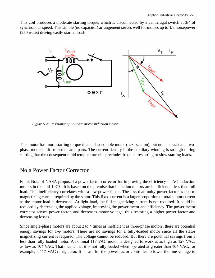
This coil produces a moderate starting torque, which is disconnected by a centrifugal switch at 3/4 of synchronous speed. This simple (no capacitor) arrangement serves well for motors up to 1/3 horsepower (250 watts) driving easily started loads.
Figure 5.25 Resistance split-phase motor induction motor
This motor has more starting torque than a shaded pole motor (next section), but not as much as a two-phase motor built from the same parts. The current density in the auxiliary winding is so high during starting that the consequent rapid temperature rise precludes frequent restarting or slow starting loads.
Nola Power Factor Corrector
Frank Nola of NASA proposed a power factor corrector for improving the efficiency of AC induction motors in the mid-1970s. It is based on the premise that induction motors are inefficient at less than full load. This inefficiency correlates with a low power factor. The less than unity power factor is due to magnetizing current required by the stator. This fixed current is a larger proportion of total motor current as the motor load is decreased. At light load, the full magnetizing current is not required. It could be reduced by decreasing the applied voltage, improving the power factor and efficiency. The power factor corrector senses power factor, and decreases motor voltage, thus restoring a higher power factor and decreasing losses.
Since single-phase motors are about 2 to 4 times as inefficient as three-phase motors, there are potential energy savings for 1-φ motors. There are no savings for a fully-loaded motor since all the stator magnetizing current is required. The voltage cannot be reduced. But there are potential savings from a less than fully loaded motor. A nominal 117 VAC motor is designed to work at as high as 127 VAC, as low as 104 VAC. That means that it is not fully loaded when operated at greater than 104 VAC, for example, a 117 VAC refrigerator. It is safe for the power factor controller to lower the line voltage to
Applied Industrial Electricity 220

104-110 VAC. The higher the initial line voltage, the greater the potential savings. Of course, if the power company delivers closer to 110 VAC, the motor will operate more efficiently without any add-on device.
Any substantially idle, 25% FLC or less, a single-phase induction motor is a candidate for a PFC. Though, it needs to operate a large number of hours per year. And the more time it idles, as in lumber saw, punch press, or conveyor, the greater the possibility of paying for the controller in a few years operation. It should be easier to pay for it by a factor of three as compared to the more efficient 3-φ-motor. The cost of a PFC cannot be recovered for a motor operating only a few hours per day.
Review
Summary: Single-phase induction motors
• Single-phase induction motors are not self-starting without an auxiliary stator
winding driven by an out of phase current of near 90°. Once started the auxiliary
winding is optional.
• The auxiliary winding of a permanent split capacitor motor has a capacitor in series
with it during starting and running.
• A capacitor-start induction motor only has a capacitor in series with the auxiliary
winding during starting.
• A capacitor-run motor typically has a large non-polarized electrolytic capacitor in
series with the auxiliary winding for starting, then a smaller non-electrolytic
capacitor during running.
• The auxiliary winding of a resistance split-phase motor develops a phase difference
versus the main winding during starting by virtue of the difference in resistance.
221 Tony R. Kuphaldt and John R. Haughery

6. REACTIVE POWER
6.1 AC Resistor Circuits
Figure 6.1 Pure resistive AC circuit: resistor voltage and current are in phase.
If we were to plot the current and voltage for a very simple AC circuit consisting of a source and a resistor (figure above), it would look something like this: (figure below)
Figure 6.2 Voltage and current “in phase” for resistive circuit.
Because the resistor simply and directly resists the flow of current at all periods of time, the waveform for the voltage drop across the resistor is exactly in phase with the waveform for the current through it. We can look at any point in time along the horizontal axis of the plot and compare those values of current and voltage with each other (any “snapshot” look at the values of a wave are referred to as instantaneous values, meaning the values at that instant in time). When the instantaneous value for the current is zero, the instantaneous voltage across the resistor is also zero. Likewise, at the moment in time where the current through the resistor is at its positive peak, the voltage across the resistor is also at its positive peak, and so on. At any given point in time along the waves, Ohm’s Law holds true for the instantaneous values of voltage and current.
222

We can also calculate the power dissipated by this resistor, and plot those values on the same graph: (figure below)
Figure 6.3 Instantaneous AC power in a pure resistive circuit is always positive.
6.2 AC Inductor Circuits
Resistors vs. Inductors
Inductors do not behave the same way as resistors do. Whereas resistors simply oppose the flow of current through them (by dropping a voltage directly proportional to the current), inductors oppose changes in current through them, by dropping a voltage directly proportional to the rate of change of current. In accordance with Lenz’s Law, this induced voltage is always of such a polarity as to try to maintain current at its present value. That is, if the current is increasing in magnitude, the induced voltage will “push against” the current flow; if the current is decreasing, the polarity will reverse and “push with” the current to oppose the decrease. This opposition to current change is called reactance, rather than resistance. Expressed mathematically, the relationship between the voltage dropped across the inductor and rate of current change through the inductor is as such:
223 Tony R. Kuphaldt and John R. Haughery

Alternating Current in a Simple Inductive Circuit
The expression di/dt is one from calculus, meaning the rate of change of instantaneous current (i) over time, in amps per second. The inductance (L) is in Henrys, and the instantaneous voltage (e), of course, is in volts. Sometimes you will find the rate of instantaneous voltage expressed as “v” instead of “e” (v = L di/dt), but it means the exact same thing. To show what happens with alternating current, let’s analyze a simple inductor circuit:
Figure 6.4 Pure inductive circuit: Inductor current lags inductor voltage by 90°.
If we were to plot the current and voltage for this very simple circuit, it would look something like this:
Figure 6.5 Pure inductive circuit, waveforms.
Remember, the voltage dropped across an inductor is a reaction against the change in current through it. Therefore, the instantaneous voltage is zero whenever the instantaneous current is at a peak (zero change, or level slope, on the current sine wave), and the instantaneous voltage is at a peak wherever the instantaneous current is at maximum change (the points of steepest slope on the current wave, where it crosses the zero line). This results in a voltage wave that is 90° out of phase with the current wave.
Applied Industrial Electricity 224

Looking at the graph, the voltage wave seems to have a “head start” on the current wave; the voltage “leads” the current and the current “lags” behind the voltage.
Current lags voltage by 90° in a pure inductive circuit.
Things get even more interesting when we plot the power for this circuit:
Figure 6.6 In a pure inductive circuit, instantaneous power may be positive or negative.
Because instantaneous power is the product of the instantaneous voltage and the instantaneous current (p=ie), the power equals zero whenever the instantaneous current or voltage is zero. Whenever the instantaneous current and voltage are both positive (above the line), the power is positive. As with the resistor example, the power is also positive when the instantaneous current and voltage are both negative (below the line). However, because the current and voltage waves are 90° out of phase, there are times when one is positive while the other is negative, resulting in equally frequent occurrences of negative instantaneous power.
What is Negative Power?
But what does negative power mean? It means that the inductor is releasing power back to the circuit, while a positive power means that it is absorbing power from the circuit. Since the positive and negative power cycles are equal in magnitude and duration over time, the inductor releases just as much power back to the circuit as it absorbs over the span of a complete cycle. What this means in a practical sense is that the reactance of an inductor dissipates net energy of zero, quite unlike the resistance of a resistor,
225 Tony R. Kuphaldt and John R. Haughery
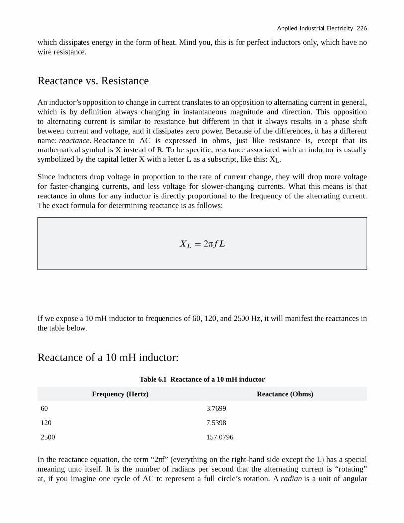
which dissipates energy in the form of heat. Mind you, this is for perfect inductors only, which have no wire resistance.
Reactance vs. Resistance
An inductor’s opposition to change in current translates to an opposition to alternating current in general, which is by definition always changing in instantaneous magnitude and direction. This opposition to alternating current is similar to resistance but different in that it always results in a phase shift between current and voltage, and it dissipates zero power. Because of the differences, it has a different name: reactance. Reactance to AC is expressed in ohms, just like resistance is, except that its mathematical symbol is X instead of R. To be specific, reactance associated with an inductor is usually symbolized by the capital letter X with a letter L as a subscript, like this: XL.
Since inductors drop voltage in proportion to the rate of current change, they will drop more voltage for faster-changing currents, and less voltage for slower-changing currents. What this means is that reactance in ohms for any inductor is directly proportional to the frequency of the alternating current. The exact formula for determining reactance is as follows:
If we expose a 10 mH inductor to frequencies of 60, 120, and 2500 Hz, it will manifest the reactances in the table below.
Reactance of a 10 mH inductor:
Table 6.1 Reactance of a 10 mH inductor
Frequency (Hertz) Reactance (Ohms)
60 3.7699
120 7.5398
2500 157.0796
In the reactance equation, the term “2πf” (everything on the right-hand side except the L) has a special meaning unto itself. It is the number of radians per second that the alternating current is “rotating” at, if you imagine one cycle of AC to represent a full circle’s rotation. A radian is a unit of angular
Applied Industrial Electricity 226

measurement: there are 2π radians in one full circle, just as there are 360° in a full circle. If the alternator producing the AC is a double-pole unit, it will produce one cycle for every full turn of shaft rotation, which is every 2π radians, or 360°. If this constant of 2π is multiplied by frequency in Hertz (cycles per second), the result will be a figure in radians per second, known as the angular velocity of the AC system.
Angular Velocity in AC Systems
Angular velocity may be represented by the expression 2πf, or it may be represented by its own symbol, the lowercase Greek letter omega, which appears similar to our Roman lower-case “w”: ω. Thus, the reactance formula XL = 2πfL could also be written as XL = ωL.
It must be understood that this “angular velocity” is an expression of how rapidly the AC waveforms are cycling, a full-cycle being equal to 2π radians. It is not necessarily representative of the actual shaft speed of the alternator producing the AC. If the alternator has more than two poles, the angular velocity will be a multiple of the shaft speed. For this reason, ω is sometimes expressed in units of electrical radians per second rather than (plain) radians per second, so as to distinguish it from mechanical motion.
Any way we express the angular velocity of the system, it is apparent that it is directly proportional to reactance in an inductor. As the frequency (or alternator shaft speed) is increased in an AC system, an inductor will offer greater opposition to the passage of current, and vice versa. Alternating current in a simple inductive circuit is equal to the voltage (in volts) divided by the inductive reactance (in ohms), just as either alternating or direct current in a simple resistive circuit is equal to the voltage (in volts) divided by the resistance (in ohms). An example circuit is shown here:
Example 6.1
Inductive reactance
227 Tony R. Kuphaldt and John R. Haughery

(Inductive reactance of 10 mH inductor at 60Hz)
Phase Angles
However, we need to keep in mind that voltage and current are not in phase here. As was shown earlier, the voltage has a phase shift of +90° with respect to the current. If we represent these phase angles of voltage and current mathematically in the form of complex numbers, we find that an inductor’s opposition to current has a phase angle, too:
Example 6.2
Applied Industrial Electricity 228

Mathematically, we say that the phase angle of an inductor’s opposition to current is 90°, meaning that an inductor’s opposition to current is a positive imaginary quantity. This phase angle of reactive opposition to current becomes critically important in circuit analysis, especially for complex AC circuits where reactance and resistance interact. It will prove beneficial to represent any component’s opposition to current in terms of complex numbers rather than scalar quantities of resistance and reactance.
Review
• Inductive reactance is the opposition that an inductor offers to alternating current
due to its phase-shifted storage and release of energy in its magnetic field.
Reactance is symbolized by the capital letter “X” and is measured in ohms just like
resistance (R).
• Inductive reactance can be calculated using this formula: XL = 2πfL
• The angular velocity of an AC circuit is another way of expressing its frequency, in
units of electrical radians per second instead of cycles per second. It is symbolized
by the lowercase Greek letter “omega,” or ω.
• Inductive reactance increases with increasing frequency. In other words, the higher
229 Tony R. Kuphaldt and John R. Haughery

the frequency, the more it opposes the AC flow of electrons.
6.3 Series Resistor Inductor Circuit
Take this circuit as an example to work with:
Series resistor inductor circuit: Current lags applied voltage by 0o to 90o.
The resistor will offer 5 Ω of resistance to AC current regardless of frequency, while the inductor will offer 3.7699 Ω of reactance to AC current at 60 Hz.
Because the resistor’s resistance is a real number (5 Ω ∠ 0°, or 5 + j0 Ω), and the inductor’s reactance is an imaginary number (3.7699 Ω ∠ 90°, or 0 + j3.7699 Ω), the combined effect of the two components will be an opposition to current equal to the complex sum of the two numbers.
This combined opposition will be a vector combination of resistance and reactance. In order to express this opposition succinctly, we need a more comprehensive term for opposition to current than either resistance or reactance alone.
This term is called impedance, its symbol is Z, and it is also expressed in the unit of ohms, just like resistance and reactance. In the above example, the total circuit impedance is:
Applied Industrial Electricity 230

Resistance in Ohm’s Law
Impedance is related to voltage and current just as you might expect, in a manner similar to resistance in Ohm’s Law:
In fact, this is a far more comprehensive form of Ohm’s Law than what was taught in DC electronics (E=IR), just as impedance is a far more comprehensive expression of opposition to the flow of current than resistance is. Any resistance and any reactance, separately or in combination (series/parallel), can be and should be represented as a single impedance in an AC circuit.
To calculate current in the above circuit, we first need to give a phase angle reference for the voltage source, which is generally assumed to be zero. (The phase angles of resistive and inductive impedance are always 0° and +90°, respectively, regardless of the given phase angles for voltage or current).
231 Tony R. Kuphaldt and John R. Haughery
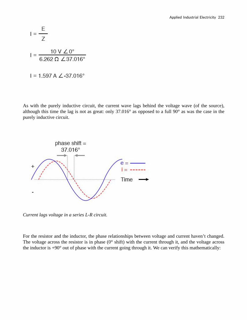
As with the purely inductive circuit, the current wave lags behind the voltage wave (of the source), although this time the lag is not as great: only 37.016° as opposed to a full 90° as was the case in the purely inductive circuit.
Current lags voltage in a series L-R circuit.
For the resistor and the inductor, the phase relationships between voltage and current haven’t changed. The voltage across the resistor is in phase (0° shift) with the current through it, and the voltage across the inductor is +90° out of phase with the current going through it. We can verify this mathematically:
Applied Industrial Electricity 232

The voltage across the resistor has the exact same phase angle as the current through it, telling us that E and I are in phase (for the resistor only).
The voltage across the inductor has a phase angle of 52.984°, while the current through the inductor has a phase angle of -37.016°, a difference of exactly 90° between the two. This tells us that E and I are still 90° out of phase (for the inductor only).
Use the Kirchhoff’s Voltage Law
We can also mathematically prove that these complex values add together to make the total voltage, just as Kirchhoff’s Voltage Law would predict:
233 Tony R. Kuphaldt and John R. Haughery

6.4 Parallel Resistor-Inductor Circuits
Let’s take the same components for our series example circuit and connect them in parallel:
Figure 6.7 Parallel R-L circuit.
Because the power source has the same frequency as the series example circuit, and the resistor and inductor both have the same values of resistance and inductance, respectively, they must also have the same values of impedance. So, we can begin our analysis table with the same “given” values:
Applied Industrial Electricity 234
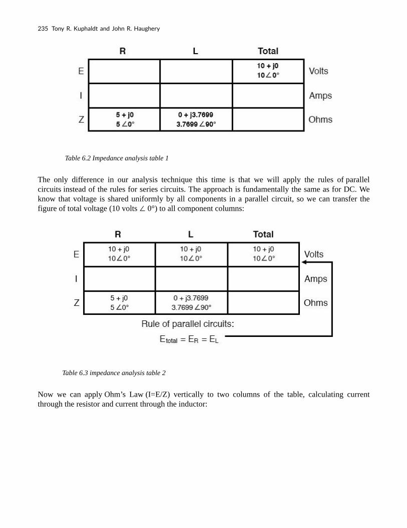
Table 6.2 Impedance analysis table 1
The only difference in our analysis technique this time is that we will apply the rules of parallel circuits instead of the rules for series circuits. The approach is fundamentally the same as for DC. We know that voltage is shared uniformly by all components in a parallel circuit, so we can transfer the figure of total voltage (10 volts ∠ 0°) to all component columns:
Table 6.3 impedance analysis table 2
Now we can apply Ohm’s Law (I=E/Z) vertically to two columns of the table, calculating current through the resistor and current through the inductor:
235 Tony R. Kuphaldt and John R. Haughery

Table 6.4 Impedance analysis table 3
Just as with DC circuits, branch currents in a parallel AC circuit add to form the total current (Kirchhoff’s Current Law still holds true for AC as it did for DC):
Table 6.5 Impedance analysis table 4
Finally, total impedance can be calculated by using Ohm’s Law (Z=E/I) vertically in the “Total” column. Incidentally, parallel impedance can also be calculated by using a reciprocal formula identical to that used in calculating parallel resistances.
Applied Industrial Electricity 236
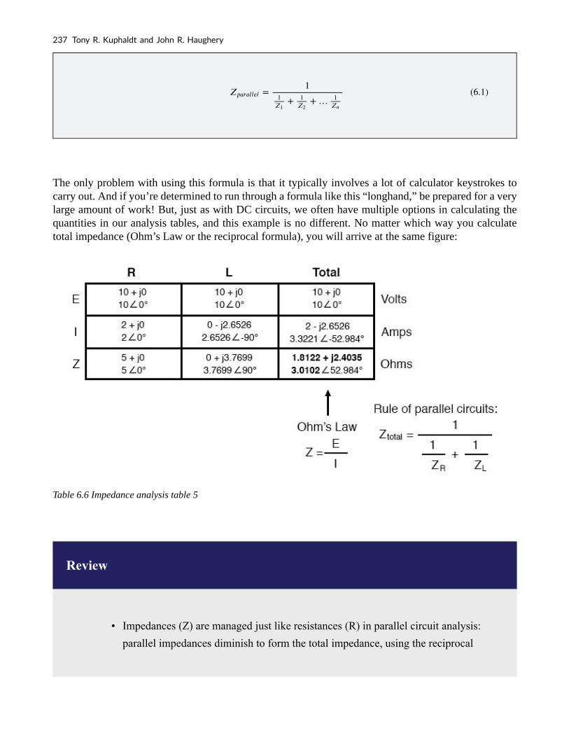
The only problem with using this formula is that it typically involves a lot of calculator keystrokes to carry out. And if you’re determined to run through a formula like this “longhand,” be prepared for a very large amount of work! But, just as with DC circuits, we often have multiple options in calculating the quantities in our analysis tables, and this example is no different. No matter which way you calculate total impedance (Ohm’s Law or the reciprocal formula), you will arrive at the same figure:
Table 6.6 Impedance analysis table 5
Review
• Impedances (Z) are managed just like resistances (R) in parallel circuit analysis:
parallel impedances diminish to form the total impedance, using the reciprocal
237 Tony R. Kuphaldt and John R. Haughery

formula. Just be sure to perform all calculations in complex (not scalar) form!
• Ohm’s Law for AC circuits:
; ;
• When resistors and inductors are mixed together in parallel circuits (just as in series
circuits), the total impedance will have a phase angle somewhere between 0° and
+90°. The circuit current will have a phase angle somewhere between 0° and -90°.
• Parallel AC circuits exhibit the same fundamental properties as parallel DC circuits:
voltage is uniform throughout the circuit, branch currents add to form the total
current, and impedances diminish (through the reciprocal formula) to form the total
impedance.
6.5 Inductor Quirks
In an ideal case, an inductor acts as a purely reactive device. That is, its opposition to AC current is strictly based on inductive reaction to changes in current, and not electron friction as is the case with resistive components. However, inductors are not quite so pure in their reactive behavior. To begin with, they’re made of wire, and we know that all wire possesses some measurable amount of resistance (unless its superconducting wire). This built-in resistance acts as though it were connected in series with the perfect inductance of the coil, like this:
Applied Industrial Electricity 238

Figure 6.8 Inductor Equivalent circuit of a real inductor.
Consequently, the impedance of any real inductor will always be a complex combination of resistance and inductive reactance.
Compounding this problem is something called the skin effect, which is AC’s tendency to flow through the outer areas of a conductor’s cross-section rather than through the middle. When electrons flow in a single direction (DC), they use the entire cross-sectional area of the conductor to move. Electrons switching directions of flow, on the other hand, tend to avoid travel through the very middle of a conductor, limiting the effective cross-sectional area available. The skin effect becomes more pronounced as frequency increases.
Also, the alternating magnetic field of an inductor energized with AC may radiate off into space as part of an electromagnetic wave, especially if the AC is of high frequency. This radiated energy does not return to the inductor, and so it manifests itself as resistance (power dissipation) in the circuit.
Added to the resistive losses of wire and radiation, there are other effects at work in iron-core inductors which manifest themselves as additional resistance between the leads. When an inductor is energized with AC, the alternating magnetic fields produced tend to induce circulating currents within the iron core known as eddy currents. These electric currents in the iron core have to overcome the electrical resistance offered by the iron, which is not as good a conductor as copper. Eddy current losses are primarily counteracted by dividing the iron core up into many thin sheets (laminations), each one separated from the other by a thin layer of electrically insulating varnish. With the cross-section of the core divided up into many electrically isolated sections, current cannot circulate within that cross-sectional area and there will be no (or very little) resistive losses from that effect.
As you might have expected, eddy current losses in metallic inductor cores manifest themselves in the form of heat. The effect is more pronounced at higher frequencies, and can be so extreme that it is sometimes exploited in manufacturing processes to heat metal objects! In fact, this process of “inductive heating” is often used in high-purity metal foundry operations, where metallic elements and alloys must
239 Tony R. Kuphaldt and John R. Haughery

be heated in a vacuum environment to avoid contamination by air, and thus where standard combustion heating technology would be useless. It is a “non-contact” technology, the heated substance not having to touch the coil(s) producing the magnetic field.
In high-frequency service, eddy currents can even develop within the cross-section of the wire itself, contributing to additional resistive effects. To counteract this tendency, special wire made of very fine, individually insulated strands called Litz wire (short for Litzendraht) can be used. The insulation separating strands from each other prevent eddy currents from circulating through the whole wire’s cross-sectional area.
Additionally, any magnetic hysteresis that needs to be overcome with every reversal of the inductor’s magnetic field constitutes an expenditure of energy that manifests itself as resistance in the circuit. Some core materials (such as ferrite) are particularly notorious for their hysteretic effect. Counteracting this effect is best done by means of proper core material selection and limits on the peak magnetic field intensity generated with each cycle.
Altogether, the stray resistive properties of a real inductor (wire resistance, radiation losses, eddy currents, and hysteresis losses) are expressed under the single term of “effective resistance:”
Figure 6.9 Equivalent circuit of a real inductor with skin-effect, radiation, eddy current, and hysteresis losses.
It is worthy to note that the skin effect and radiation losses apply just as well to straight lengths of wire in an AC circuit as they do a coiled wire. Usually, their combined effect is too small to notice, but at radio frequencies, they can be quite large. A radio transmitter antenna, for example, is designed with the express purpose of dissipating the greatest amount of energy in the form of electromagnetic radiation.
Applied Industrial Electricity 240

6.6 AC Capacitor Circuits
Capacitors Vs. Resistors
Capacitors do not behave the same as resistors. Whereas resistors allow a flow of electrons through them directly proportional to the voltage drop, capacitors oppose changes in voltage by drawing or supplying current as they charge or discharge to the new voltage level. The flow of electrons “through” a capacitor is directly proportional to the rate of change of voltage across the capacitor. This opposition to voltage change is another form of reactance, but one that is precisely opposite to the kind exhibited by inductors.
Capacitor Circuit Characteristics
Expressed mathematically, the relationship between the current “through” the capacitor and rate of voltage change across the capacitor is as such:
The expression de/dt is one from calculus, meaning the rate of change of instantaneous voltage (e) over time, in volts per second. The capacitance (C) is in Farads, and the instantaneous current (i), of course, is in amps. Sometimes you will find the rate of instantaneous voltage change over time expressed as dv/dt instead of de/dt: using the lower-case letter “v” instead or “e” to represent voltage, but it means the exact same thing. To show what happens with alternating current, let’s analyze a simple capacitor circuit:
241 Tony R. Kuphaldt and John R. Haughery

Figure 6.10 Pure capacitive circuit: capacitor voltage lags capacitor current by 90°
If we were to plot the current and voltage for this very simple circuit, it would look something like this:
Figure 6.11 Pure capacitive circuit waveforms.
Remember, the current through a capacitor is a reaction against the change in voltage across it. Therefore, the instantaneous current is zero whenever the instantaneous voltage is at a peak (zero change, or level slope, on the voltage sine wave), and the instantaneous current is at a peak wherever the instantaneous voltage is at maximum change (the points of steepest slope on the voltage wave, where it crosses the zero line). This results in a voltage wave that is -90° out of phase with the current wave. Looking at the graph, the current wave seems to have a “head start” on the voltage wave; the current “leads” the voltage, and the voltage “lags” behind the current.
Figure 6.12 Voltage lags current by 90° in a pure capacitive circuit.
Applied Industrial Electricity 242

As you might have guessed, the same unusual power wave that we saw with the simple inductor circuit is present in the simple capacitor circuit, too:
Figure 6.13 In a pure capacitive circuit, the instantaneous power may be positive or negative.
As with the simple inductor circuit, the 90-degree phase shift between voltage and current results in a power wave that alternates equally between positive and negative. This means that a capacitor does not dissipate power as it reacts against changes in voltage; it merely absorbs and releases power, alternately.
A Capacitor’s Reactance
A capacitor’s opposition to change in voltage translates to an opposition to alternating voltage in general, which is by definition always changing in instantaneous magnitude and direction. For any given magnitude of AC voltage at a given frequency, a capacitor of given size will “conduct” a certain magnitude of AC current. Just as the current through a resistor is a function of the voltage across the resistor and the resistance offered by the resistor, the AC current through a capacitor is a function of the AC voltage across it, and the reactance offered by the capacitor. As with inductors, the reactance of a capacitor is expressed in ohms and symbolized by the letter X (or XC to be more specific).
Since capacitors “conduct” current in proportion to the rate of voltage change, they will pass more current for faster-changing voltages (as they charge and discharge to the same voltage peaks in less time), and less current for slower-changing voltages. What this means is that reactance in ohms for any capacitor is inversely proportional to the frequency of the alternating current.
243 Tony R. Kuphaldt and John R. Haughery

Reactance of a 100 uF capacitor:
Frequency (Hertz) Reactance (Ohms)
60 26.5258
120 13.2629
2500 0.6366
Please note that the relationship of capacitive reactance to frequency is exactly opposite from that of inductive reactance. Capacitive reactance (in ohms) decreases with increasing AC frequency. Conversely, inductive reactance (in ohms) increases with increasing AC frequency. Inductors oppose faster changing currents by producing greater voltage drops; capacitors oppose faster changing voltage drops by allowing greater currents.
As with inductors, the reactance equation’s 2πf term may be replaced by the lowercase Greek letter Omega (ω), which is referred to as the angular velocity of the AC circuit. Thus, the equation XC = 1/(2πfC) could also be written as XC = 1/(ωC), with ω cast in units of radians per second.
Alternating current in a simple capacitive circuit is equal to the voltage (in volts) divided by the capacitive reactance (in ohms), just as either alternating or direct current in a simple resistive circuit is equal to the voltage (in volts) divided by the resistance (in ohms). The following circuit illustrates this mathematical relationship by example:
Examples 6.3
Capacitive reactance.
Applied Industrial Electricity 244

However, we need to keep in mind that voltage and current are not in phase here. As was
shown earlier, the current has a phase shift of +90° with respect to the voltage. If we represent
these phase angles of voltage and current mathematically, we can calculate the phase angle of
the capacitor’s reactive opposition to current.
245 Tony R. Kuphaldt and John R. Haughery

Voltage lags current by 90° in a capacitor.
Mathematically, we say that the phase angle of a capacitor’s opposition to current is -90°, meaning that a capacitor’s opposition to current is a negative imaginary quantity. (See figure above.) This phase angle of reactive opposition to current becomes critically important in circuit analysis, especially for complex AC circuits where reactance and resistance interact. It will prove beneficial to represent any component’s opposition to current in terms of complex numbers, and not just scalar quantities of resistance and reactance.
Review
• Capacitive reactance is the opposition that a capacitor offers to alternating current
due to its phase-shifted storage and release of energy in its electric field. Reactance
is symbolized by the capital letter “X” and is measured in ohms just like resistance
(R).
• Capacitive reactance can be calculated using this formula: XC = 1/(2πfC)
• Capacitive reactance decreases with increasing frequency. In other words, the
higher the frequency, the less it opposes (the more it “conducts”) AC current.
Applied Industrial Electricity 246

6.7 Parallel Resistor-Capacitor Circuits
Using the same value components in our series example circuit, we will connect them in parallel and see what happens:
Figure 6.14 Parallel R-C circuit.
Resistor and Capacitor in Parallel
Because the power source has the same frequency as the series example circuit, and the resistor and capacitor both have the same values of resistance and capacitance, respectively, they must also have the same values of impedance. So, we can begin our analysis table with the same “given” values:
Table 6.7
This being a parallel circuit now, we know that voltage is shared equally by all components, so we can place the figure for total voltage (10 volts ∠ 0°) in all the columns:
247 Tony R. Kuphaldt and John R. Haughery

Table 6.8
Calculation Using Ohm’s Law
Now we can apply Ohm’s Law (I=E/Z) vertically to two columns in the table, calculating current through the resistor and current through the capacitor:
Table 6.9
Just as with DC circuits, branch currents in a parallel AC circuit add up to form the total current (Kirchhoff’s Current Law again):
Applied Industrial Electricity 248

Table 6.10
Finally, total impedance can be calculated by using Ohm’s Law (Z=E/I) vertically in the “Total” column. As we saw in the AC inductance chapter, parallel impedance can also be calculated by using a reciprocal formula identical to that used in calculating parallel resistances. It is noteworthy to mention that this parallel impedance rule holds true regardless of the kind of impedances placed in parallel. In other words, it doesn’t matter if we’re calculating a circuit composed of parallel resistors, parallel inductors, parallel capacitors, or some combination thereof: in the form of impedances (Z), all the terms are common and can be applied uniformly to the same formula. Once again, the parallel impedance formula looks like this:
The only drawback to using this equation is the significant amount of work required to work it out, especially without the assistance of a calculator capable of manipulating complex quantities. Regardless of how we calculate total impedance for our parallel circuit (either Ohm’s Law or the reciprocal formula), we will arrive at the same figure:
• Impedances (Z) are managed just like resistances (R) in parallel circuit analysis: parallel impedances diminish to form the total impedance, using the reciprocal formula. Just be sure
249 Tony R. Kuphaldt and John R. Haughery
to
Review
◦ perform all calculations in complex (not scalar) form! ZTotal = 1/(1/Z1 +
1/Z2 + . . . 1/Zn)
◦ Ohm’s Law for AC circuits: E = IZ ; I = E/Z ; Z = E/I
◦ When resistors and capacitors are mixed together in parallel circuits (just
as in series circuits), the total impedance will have a phase angle
somewhere between 0° and -90°. The circuit current will have a phase
angle somewhere between 0° and +90°.
◦ Parallel AC circuits exhibit the same fundamental properties as parallel
DC circuits: voltage is uniform throughout the circuit, branch currents add
to form the total current, and impedances diminish (through the reciprocal
formula) to form the total impedance.
6.8 Review of R, X, and Z
(The following section was adapted from: Lessons in Electric Circuits, Vol II, Chapter 5 – Reactance And Impedance — R, L, And C)
Before we begin to explore the effects of resistors, inductors, and capacitors connected together in the same AC circuits, let’s briefly review some basic terms and facts.
Resistance
This is essentially friction against the flow of current. It is present in all conductors to some extent (except superconductors!), most notably in resistors. When the alternating current goes through a resistance, a voltage drop is produced that is in-phase with the current. Resistance is mathematically symbolized by the letter “R” and is measured in the unit of ohms (Ω).
Applied Industrial Electricity 250

Reactance
This is essentially inertia against the flow of current. It is present anywhere electric or magnetic fields are developed in proportion to an applied voltage or current, respectively; but most notably in capacitors and inductors. When the alternating current goes through a pure reactance, a voltage drop is produced that is 90° out of phase with the current. Reactance is mathematically symbolized by the letter “X” and is measured in the unit of ohms (Ω).
Impedance
This is a comprehensive expression of any and all forms of opposition to current flow, including both resistance and reactance. It is present in all circuits, and in all components. When the alternating current goes through an impedance, a voltage drop is produced that is somewhere between 0° and 90° out of phase with the current. Impedance is mathematically symbolized by the letter “Z” and is measured in the unit of ohms (Ω), in complex form.
Perfect resistors possess resistance, but not reactance. Perfect inductors and perfect capacitors possess reactance but no resistance. All components possess impedance, and because of this universal quality, it makes sense to translate all component values (resistance, inductance, capacitance) into common terms of impedance as the first step in analyzing an AC circuit.
Figure 6.15 Perfect resistor, inductor, and capacitor.
The impedance phase angle for any component is the phase shift between the voltage across that component and current through that component. For a perfect resistor, the voltage drop and current are always in phase with each other, and so the impedance angle of a resistor is said to be 0°. For a perfect inductor, voltage drop always leads current by 90°, and so an inductor’s impedance phase angle is said to be +90°. For a perfect capacitor, voltage drop always lags current by 90°, and so a capacitor’s impedance phase angle is said to be -90°.
251 Tony R. Kuphaldt and John R. Haughery

Impedances in AC behave analogously to resistances in DC circuits: they add in series, and they diminish in parallel. A revised version of Ohm’s Law, based on impedance rather than resistance, looks like this:
Ohm’s Law for AC Circuit
6.9 Parallel R, L, and C
We can take the same components from the series circuit and rearrange them into a parallel configuration for an easy example circuit:
Figure 6.16 Example R, L, and C parallel circuit.
Impedance in Parallel Components
The fact that these components are connected in parallel instead of series now has absolutely no effect on their individual impedances. So long as the power supply is the same frequency as before, the inductive and capacitive reactances will not have changed at all.
Applied Industrial Electricity 252

Figure 6.17 Example R, L, and C parallel circuit with impedances replacing component values.
With all component values expressed as impedances (Z), we can set up an analysis table and proceed as in the last example problem, except this time following the rules of parallel circuits instead of series.
Knowing that voltage is shared equally by all components in a parallel circuit, we can transfer the figure for total voltage to all component columns in the table:
Table 6.11 components values express as impedance image 2
Now, we can apply Ohm’s Law (I=E/Z) vertically in each column to determine the current through each component:
253 Tony R. Kuphaldt and John R. Haughery

Table 6.12 components values express as impedance image 3
Calculation of Total Current and Total Impedance
There are two strategies for calculating the total current and total impedance. First, we could calculate total impedance from all the individual impedances in parallel (ZTotal = 1/(1/ZR + 1/ZL + 1/ZC), and then calculate total current by dividing source voltage by total impedance (I=E/Z).
However, working through the parallel impedance equation with complex numbers is no easy task, with all the reciprocations (1/Z). This is especially true if you’re unfortunate enough not to have a calculator that handles complex numbers and are forced to do it all by hand (reciprocate the individual impedances in polar form, then convert them all to rectangular form for addition, then convert back to polar form for the final inversion, then invert). The second way to calculate total current and total impedance is to add up all the branch currents to arrive at total current (total current in a parallel circuit—AC or DC—is equal to the sum of the branch currents), then use Ohm’s Law to determine total impedance from total voltage and total current (Z=E/I).
Table 6.13 Calculation of total current and total impedance
Either method, performed properly, will provide the correct answers.
Applied Industrial Electricity 254

6.10 R, L and C Summary
With the notable exception of calculations for power (P), all AC circuit calculations are based on the same general principles as calculations for DC circuits. The only significant difference is that fact that AC calculations use complex quantities while DC calculations use scalar quantities. Ohm’s Law, Kirchhoff’s Laws, and even the network theorems learned in DC still hold true for AC when voltage, current, and impedance are all expressed with complex numbers. The same troubleshooting strategies applied toward DC circuits also hold for AC, although AC can certainly be more difficult to work with due to phase angles which aren’t registered by a handheld multimeter.
Power is another subject altogether and will be covered in its own chapter in this book. Because the power in a reactive circuit is both absorbed and released—not just dissipated as it is with resistors—its mathematical handling requires a more direct application of trigonometry to solve.
When faced with analyzing an AC circuit, the first step in the analysis is to convert all resistor, inductor, and capacitor component values into impedances (Z), based on the frequency of the power source. After, proceed with the same steps and strategies learned for analyzing DC circuits, using the new form of Ohm’s Law: E=IZ; I=E/Z; and Z=E/I
Remember that only the calculated figures expressed in polar form apply directly to empirical measurements of voltage and current. A rectangular notation is merely a useful tool for us to add and subtract complex quantities together. Polar notation, where the magnitude (length of the vector) directly relates to the magnitude of the voltage or current measured, and the angle directly relates to the phase shift in degrees, is the most practical way to express complex quantities for circuit analysis.
255 Tony R. Kuphaldt and John R. Haughery

7. POWER FACTOR CORRECTION
7.1 Power in Resistive and Reactive AC circuits
Example 7.1
Consider a circuit for a single-phase AC power system, where a 120 volt, 60 Hz AC voltage
source is delivering power to a resistive load: (Figure below)
Ac source drives a purely resistive load.
Z =60 + j0 \Omega \textbf{ or } 60\Omega \angle \text{ 0°}
256

In this example, the current to the load would be 2 amps, RMS. The power dissipated at the load would be 240 watts. Because this load is purely resistive (no reactance), the current is in phase with the voltage, and calculations look similar to that in an equivalent DC circuit. If we were to plot the voltage, current, and power waveforms for this circuit, it would look like the figure below.
Figure 7.1 Current is in phase with voltage in a resistive circuit.
Note that the waveform for power is always positive, never negative for this resistive circuit. This means that power is always being dissipated by the resistive load, and never returned to the source as it is with reactive loads. If the source were a mechanical generator, it would take 240 watts worth of mechanical energy (about 1/3 horsepower) to turn the shaft.
Also, note that the waveform for power is not at the same frequency as the voltage or current! Rather, its frequency is double that of either the voltage or current waveforms. This different frequency prohibits our expression of power in an AC circuit using the same complex (rectangular or polar) notation as used for voltage, current, and impedance because this form of mathematical symbolism implies unchanging phase relationships. When frequencies are not the same, phase relationships constantly change.
257 Tony R. Kuphaldt and John R. Haughery
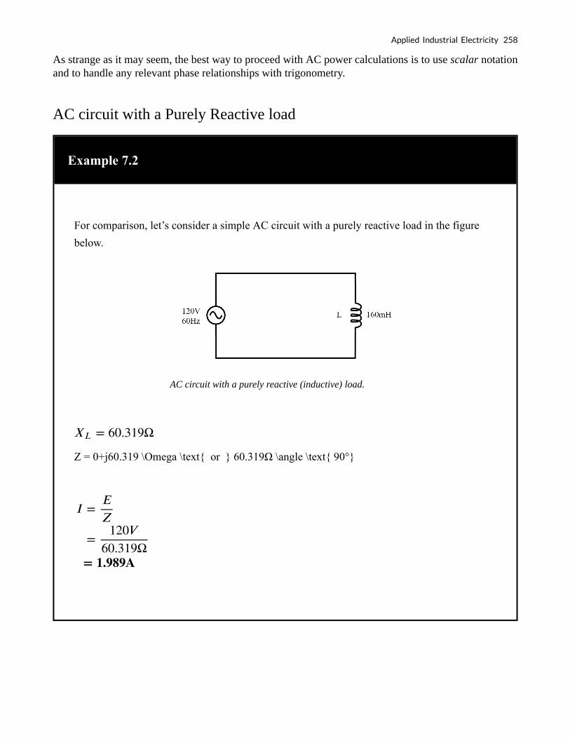
As strange as it may seem, the best way to proceed with AC power calculations is to use scalar notation and to handle any relevant phase relationships with trigonometry.
AC circuit with a Purely Reactive load
Example 7.2
For comparison, let’s consider a simple AC circuit with a purely reactive load in the figure
below.
AC circuit with a purely reactive (inductive) load.
Z = 0+j60.319 \Omega \text{ or } 60.319Ω \angle \text{ 90°}
Applied Industrial Electricity 258

Figure 7.2 Power is not dissipated in a purely reactive load. Though it is alternately absorbed from and returned to the source.
Note that the power alternates equally between cycles of positive and negative. (Figure above) This means that power is being alternately absorbed from and returned to the source. If the source were a mechanical generator, it would take (practically) no net mechanical energy to turn the shaft, because no power would be used by the load. The generator shaft would be easy to spin, and the inductor would not become warm as a resistor would.
AC circuit with a Resistive and Purely Reactive load
Example 7.3
Now, let’s consider an AC circuit with a load consisting of both inductance and resistance in
the figure below.
259 Tony R. Kuphaldt and John R. Haughery

circuit with both reactance and resistance.
or
or
or
At a frequency of 60 Hz, the 160 millihenrys of inductance give us 60.319 Ω of inductive reactance. This reactance combines with the 60 Ω of resistance to form a total load impedance of 60 + j60.319 Ω, or 85.078 Ω ∠ 45.152o. If we’re not concerned with phase angles (which we’re not at this point), we may calculate current in the circuit by taking the polar magnitude of the voltage source (120 volts) and dividing it by the polar magnitude of the impedance (85.078 Ω). With a power supply voltage of 120 volts RMS, our load current is 1.410 amps. This is the figure an RMS ammeter would indicate if connected in series with the resistor and inductor.
Applied Industrial Electricity 260

We already know that reactive components dissipate zero power, as they equally absorb power from, and return power to, the rest of the circuit. Therefore, any inductive reactance in this load will likewise dissipate zero power. The only thing left to dissipate power here is the resistive portion of the load impedance. If we look at the waveform plot of voltage, current, and total power for this circuit, we see how this combination works in the figure below.
Figure 7.3 A combined resistive/reactive circuit dissipates more power than it returns to the source. The reactance dissipates no power; though, the resistor does.
As with any reactive circuit, the power alternates between positive and negative instantaneous values over time. In a purely reactive circuit that alternation between positive and negative power is equally divided, resulting in net power dissipation of zero. However, in circuits with mixed resistance and reactance like this one, the power waveform will still alternate between positive and negative, but the amount of positive power will exceed the amount of negative power. In other words, the combined inductive/resistive load will consume more power than it returns back to the source.
Looking at the waveform plot for power, it should be evident that the wave spends more time on the positive side of the centerline than on the negative, indicating that there is more power absorbed by the load than there is returned to the circuit. What little returning of power that occurs is due to the reactance; the imbalance of positive versus negative power is due to the resistance as it dissipates energy outside of the circuit (usually in the form of heat). If the source were a mechanical generator, the amount of mechanical energy needed to turn the shaft would be the amount of power averaged between the positive and negative power cycles.
Mathematically representing power in an AC circuit is a challenge, because the power wave isn’t at the same frequency as voltage or current. Furthermore, the phase angle for power means something quite different from the phase angle for either voltage or current. Whereas the angle for voltage or current represents a relative shift in timing between two waves, the phase angle for power represents a ratio between power dissipated and power returned. Because of this way in which AC power differs from AC voltage or current, it is actually easier to arrive at figures for power by calculating with scalar quantities of voltage, current, resistance, and reactance than it is to try to derive it from vector, or complex quantities of voltage, current, and impedance that we’ve worked with so far.
261 Tony R. Kuphaldt and John R. Haughery

Review
• In a purely resistive circuit, all circuit power is dissipated by the resistor(s). Voltage
and current are in phase with each other.
• In a purely reactive circuit, no circuit power is dissipated by the load(s). Rather,
power is alternately absorbed from and returned to the AC source. Voltage and
current are 90° out of phase with each other.
• In a circuit consisting of resistance and reactance mixed, there will be more power
dissipated by the load(s) than returned, but some power will definitely be dissipated
and some will merely be absorbed and returned. Voltage and current in such a
circuit will be out of phase by a value somewhere between 0° and 90°.
7.2 True, Reactive, and Apparent Power
Reactive Power
We know that reactive loads such as inductors and capacitors dissipate zero power, yet the fact that they drop voltage and draw current gives the deceptive impression that they actually do dissipate power. This “phantom power” is called reactive power, and it is measured in a unit called Volt-Amps-Reactive (VAR), rather than watts. The mathematical symbol for reactive power is (unfortunately) the capital letter Q.
True Power
The actual amount of power being used, or dissipated, in a circuit is called true power, and it is measured in watts (symbolized by the capital letter P, as always).
Applied Industrial Electricity 262

Apparent Power
The combination of reactive power and true power is called apparent power, and it is the product of a circuit’s voltage and current, without reference to phase angle. Apparent power is measured in the unit of Volt-Amps (VA) and is symbolized by the capital letter S.
Calculating for Reactive, True, or Apparent Power
As a rule, true power is a function of a circuit’s dissipative elements, usually resistances (R). Reactive power is a function of a circuit’s reactance (X). Apparent power is a function of a circuit’s total impedance (Z). Since we’re dealing with scalar quantities for power calculation, any complex starting quantities such as voltage, current, and impedance must be represented by their polar magnitudes, not by real or imaginary rectangular components. For instance, if I’m calculating true power from current and resistance, I must use the polar magnitude for current, and not merely the “real” or “imaginary” portion of the current. If I’m calculating apparent power from voltage and impedance, both of these formerly complex quantities must be reduced to their polar magnitudes for the scalar arithmetic.
Equations Using Scalar Quantities
There are several power equations relating the three types of power to resistance, reactance, and impedance (all using scalar quantities):
True Power
Measured in units of Watts(w)
263 Tony R. Kuphaldt and John R. Haughery

Reactive Power
Measured in units of Volts-Amps-Reactive (VAR)
Apparent Power
Measured in units of Volts-Amps (VA)
Please note that there are two equations each for the calculation of true and reactive power. There are three equations available for the calculation of apparent power, P=IE being useful only for that purpose. Examine the following circuits and see how these three types of power interrelate for: a purely resistive load, a purely reactive load, and a resistive/reactive load.
Example 7.4
Applied Industrial Electricity 264

Resistive Load Only
True power, reactive power, and apparent power for a purely resistive load.
Example 7.5
265 Tony R. Kuphaldt and John R. Haughery

Reactive Load Only
True power, reactive power, and apparent power for a purely resistive load.
Example 7.6
Applied Industrial Electricity 266

Resistive/Reactive Load
True power, reactive power, and apparent power for a resistive/reactive load.
267 Tony R. Kuphaldt and John R. Haughery

The Power Triangle
These three types of power—true, reactive, and apparent—relate to one another in trigonometric form. We call this the power triangle: (Figure below).
Figure 7.4 Power triangle relating appearant power to true power and reactive power.
Using the laws of trigonometry, we can solve for the length of any side (amount of any type of power), given the lengths of the other two sides, or the length of one side and an angle.
Review
Applied Industrial Electricity 268

• The power dissipated by a load is referred to as true power. True power is
symbolized by the letter P and is measured in the unit of Watts (W).
• Power merely absorbed and returned in load due to its reactive properties is referred
to as reactive power. Reactive power is symbolized by the letter Q and is measured
in the unit of Volt-Amps-Reactive (VAR).
• Total power in an AC circuit, both dissipated and absorbed/returned is referred to
as apparent power. Apparent power is symbolized by the letter S and is measured in
the unit of Volt-Amps (VA).
• These three types of power are trigonometrically related to one another. In a right
triangle, P = adjacent length, Q = opposite length, and S = hypotenuse length. The
opposite angle is equal to the circuit’s impedance (Z) phase angle.
7.3 Calculating Power Factor
As was mentioned before, the angle of this “power triangle” graphically indicates the ratio between the amount of dissipated (or consumed) power and the amount of absorbed/returned power. It also happens to be the same angle as that of the circuit’s impedance in polar form. When expressed as a fraction, this ratio between true power and apparent power is called the power factor for this circuit. Because true power and apparent power form the adjacent and hypotenuse sides of a right triangle, respectively, the power factor ratio is also equal to the cosine of that phase angle. Using values from the last example circuit:
269 Tony R. Kuphaldt and John R. Haughery

Power Factor
Example 7.7
It should be noted that power factor, like all ratio measurements, is a unitless quantity.
Power Factor Values
For the purely resistive circuit, the power factor is 1 (perfect), because the reactive power equals zero. Here, the power triangle would look like a horizontal line, because the opposite (reactive power) side would have zero length.
For the purely inductive circuit, the power factor is zero, because true power equals zero. Here, the power triangle would look like a vertical line, because the adjacent (true power) side would have zero length.
Applied Industrial Electricity 270

The same could be said for a purely capacitive circuit. If there are no dissipative (resistive) components in the circuit, then the true power must be equal to zero, making any power in the circuit purely reactive. The power triangle for a purely capacitive circuit would again be a vertical line (pointing down instead of up as it was for the purely inductive circuit).
Importance of Power Factor
Power factor can be an important aspect to consider in an AC circuit because of any power factor less than 1 means that the circuit’s wiring has to carry more current than what would be necessary with zero reactance in the circuit to deliver the same amount of (true) power to the resistive load. If our last example circuit had been purely resistive, we would have been able to deliver a full 169.256 watts to the load with the same 1.410 amps of current, rather than the mere 119.365 watts that it is presently dissipating with that same current quantity. The poor power factor makes for an inefficient power delivery system.
Poor Power Factor
Poor power factor can be corrected, paradoxically, by adding another load to the circuit drawing an equal and opposite amount of reactive power, to cancel out the effects of the load’s inductive reactance. Inductive reactance can only be canceled by capacitive reactance, so we have to add a capacitor in parallel to our example circuit as the additional load. The effect of these two opposing reactances in parallel is to bring the circuit’s total impedance equal to its total resistance (to make the impedance phase angle equal, or at least closer, to zero).
Example 7.8
Since we know that the (uncorrected) reactive power is 119.998 VAR (inductive), we need to
calculate the correct capacitor size to produce the same quantity of (capacitive) reactive
power. Since this capacitor will be directly in parallel with the source (of known voltage),
we’ll use the power formula which starts from voltage and reactance:
Solving for X:
271 Tony R. Kuphaldt and John R. Haughery

Solving for C:
Let’s use a rounded capacitor value of 22 µF and see what happens to our circuit: (Figure
below)
or
Applied Industrial Electricity 272

The power factor for the circuit, overall, has been substantially improved. The main current
has been decreased from 1.41 amps to 994.7 milliamps, while the power dissipated at the load
resistor remains unchanged at 119.365 watts. The power factor is much closer to being 1:
Since the impedance angle is still a positive number, we know that the circuit, overall, is still
more inductive than it is capacitive. If our power factor correction efforts had been perfectly
on-target, we would have arrived at an impedance angle of exactly zero, or purely resistive. If
we had added too large of a capacitor in parallel, we would have ended up with an impedance
angle that was negative, indicating that the circuit was more capacitive than inductive.
It should be noted that too much capacitance in an AC circuit will result in a low power factor just as well as too much inductance. You must be careful not to over-correct when adding capacitance to an AC circuit. You must also be very careful to use the proper capacitors for the job (rated adequately for power system voltages and the occasional voltage spike from lightning strikes, for continuous AC service, and capable of handling the expected levels of current).
If a circuit is predominantly inductive, we say that its power factor is lagging (because the current wave for the circuit lags behind the applied voltage wave). Conversely, if a circuit is predominantly capacitive, we say that its power factor is leading. Thus, our example circuit started out with a power factor of 0.705 lagging and was corrected to a power factor of 0.999 lagging.
Review
273 Tony R. Kuphaldt and John R. Haughery
The poor power factor in an AC circuit may be “corrected”, or re-established at a value close to
1, by adding a parallel reactance opposite the effect of the load’s reactance. If the load’s
reactance is inductive in nature (which is almost always will be), parallel capacitance is what is
needed to correct poor power factor.
7.4 Practical Power Factor Correction
When the need arises to correct for poor power factor in an AC power system, you probably won’t have the luxury of knowing the load’s exact inductance in henrys to use for your calculations. You may be fortunate enough to have an instrument called a power factor meter to tell you what the power factor is (a number between 0 and 1), and the apparent power (which can be figured by taking a voltmeter reading in volts and multiplying by an ammeter reading in amps). In less favorable circumstances, you may have to use an oscilloscope to compare voltage and current waveforms, measuring phase shift in degrees and calculating power factor by the cosine of that phase shift. Most likely, you will have access to a wattmeter for measuring true power, whose reading you can compare against a calculation of apparent power (from multiplying total voltage and total current measurements). From the values of true and apparent power, you can determine reactive power and power factor.
Example 7.9
Let’s do an example problem to see how this works: (Figure below)
Applied Industrial Electricity 274

How to Calculate the Apparent Power in kVA
First, we need to calculate the apparent power in kVA. We can do this by multiplying load
voltage by load current:
As we can see, 2.308 kVA is a much larger figure than 1.5 kW, which tells us that the power
factor in this circuit is rather poor (substantially less than 1). Now, we figure the power factor
of this load by dividing the true power by the apparent power:
275 Tony R. Kuphaldt and John R. Haughery

Using this value for power factor, we can draw a power triangle, and from that determine the
reactive power of this load: (Figure below)Reactive power may be calculated from true
power and apparent power.
Applied Industrial Electricity 276
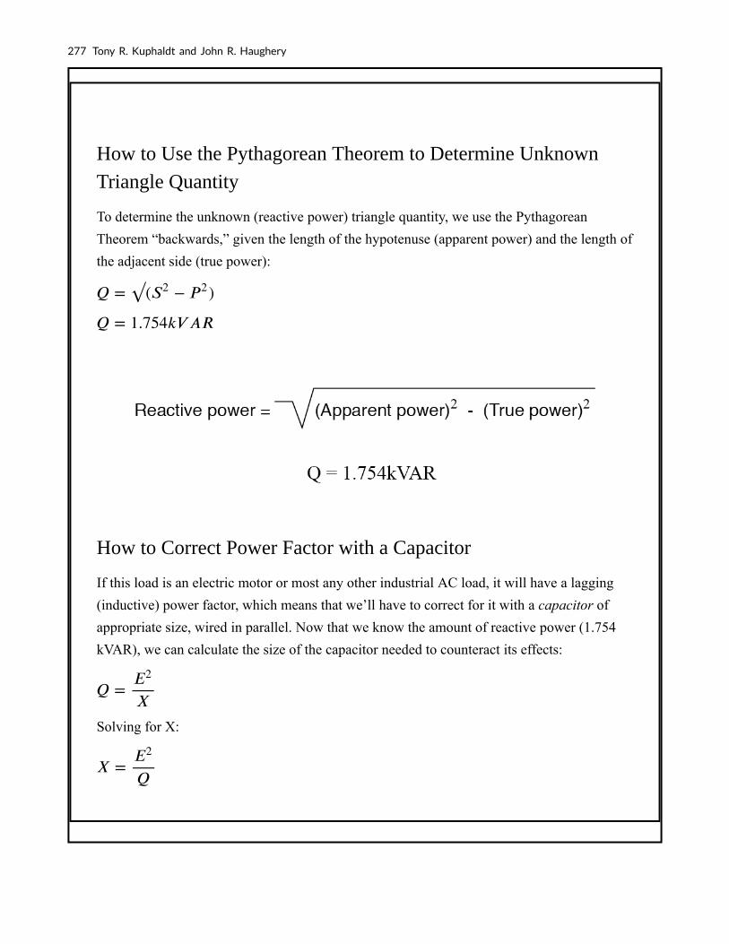
How to Use the Pythagorean Theorem to Determine Unknown
Triangle Quantity
To determine the unknown (reactive power) triangle quantity, we use the Pythagorean
Theorem “backwards,” given the length of the hypotenuse (apparent power) and the length of
the adjacent side (true power):
How to Correct Power Factor with a Capacitor
If this load is an electric motor or most any other industrial AC load, it will have a lagging
(inductive) power factor, which means that we’ll have to correct for it with a capacitor of
appropriate size, wired in parallel. Now that we know the amount of reactive power (1.754
kVAR), we can calculate the size of the capacitor needed to counteract its effects:
Solving for X:
277 Tony R. Kuphaldt and John R. Haughery

Solving for C:
Rounding this answer off to 80 µF, we can place that size of the capacitor in the circuit and
calculate the results: (Figure below)
An 80 µF capacitor will have a capacitive reactance of 33.157 Ω, giving a current of 7.238
amps, and a corresponding reactive power of 1.737 kVAR (for the capacitor only). Since the
capacitor’s current is 180o out of phase from the load’s inductive contribution to current
Applied Industrial Electricity 278
draw, the capacitor’s reactive power will directly subtract from the load’s reactive power,
resulting in:
This correction, of course, will not change the amount of true power consumed by the load,
but it will result in a substantial reduction of apparent power, and of the total current drawn
from the 240 Volt source: (Figure below)
279 Tony R. Kuphaldt and John R. Haughery
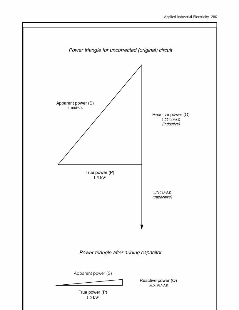
Applied Industrial Electricity 280
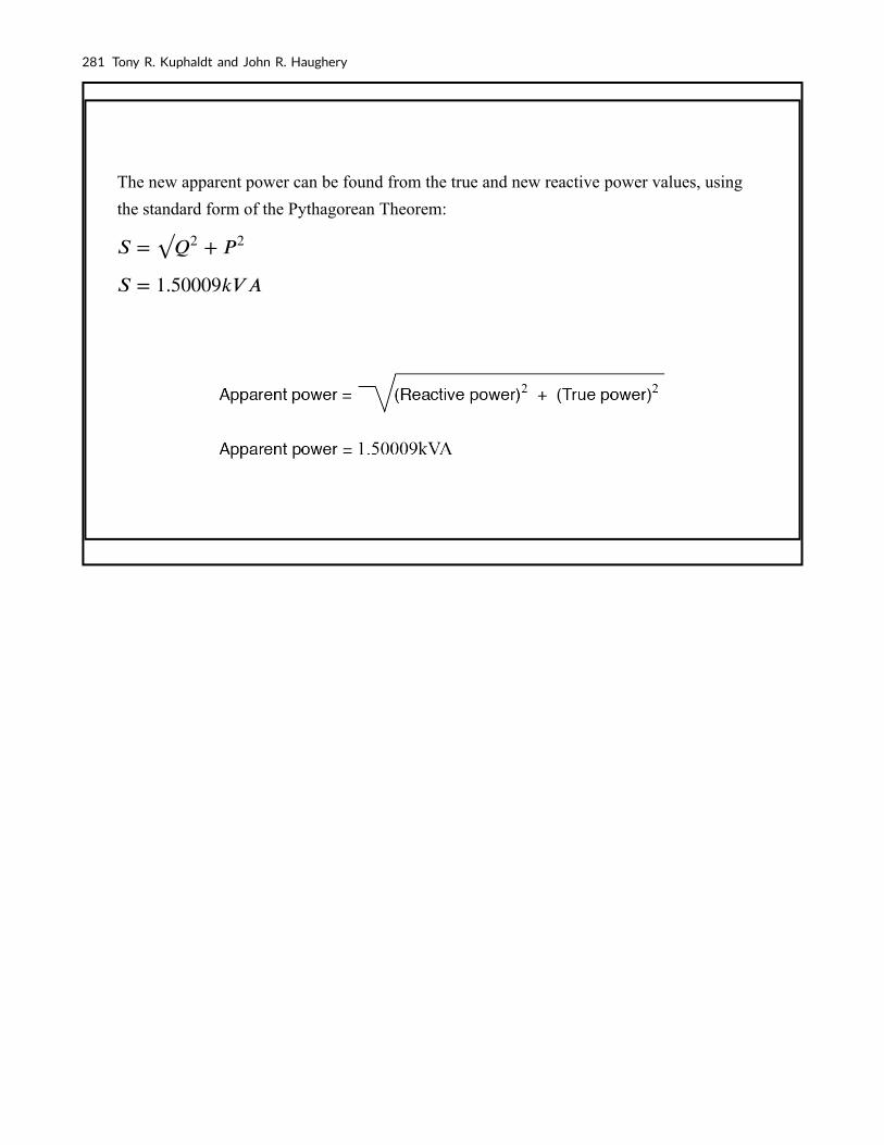
The new apparent power can be found from the true and new reactive power values, using
the standard form of the Pythagorean Theorem:
281 Tony R. Kuphaldt and John R. Haughery
8. TRANSFORMERS
8.1 Step-up and Step-down Transformers
What is Step-up and Step-down Transformers
This is a very useful device, indeed. With it, we can easily multiply or divide voltage and current in AC circuits. Indeed, the transformer has made the long-distance transmission of electric power a practical reality, as AC voltage can be “stepped up” and current “stepped down” for reduced wire resistance power losses along power lines connecting generating stations with loads. At either end (both the generator and at the loads), voltage levels are reduced by transformers for safer operation and less expensive equipment.
A transformer that increases the voltage from primary to secondary (more secondary winding turns than primary winding turns) is called a step-up transformer.
Conversely, a transformer designed to do just the opposite is called a step-down transformer.
Let’s re-examine a photograph shown in the previous section:
282

Figure 8.1 Transformer cross-section showing primary and secondary windings is a few inches tall (approximately 10 cm).
This is a step-down transformer, as evidenced by the high turn count of the primary winding and the low turn count of the secondary. As a step-down unit, this transformer converts high-voltage, low-current power into low-voltage, high-current power. The larger-gauge wire used in the secondary winding is necessary due to the increase in current. The primary winding, which doesn’t have to conduct as much current, may be made of smaller-gauge wire.
Reversibility of Transformer Operation
In case you were wondering, it is possible to operate either of these transformer types backward (powering the secondary winding with an AC source and letting the primary winding power a load) to perform the opposite function: a step-up can function as a step-down and visa-Versa.
However, as we saw in the first section of this chapter, efficient operation of a transformer requires that the individual winding inductances be engineered for specific operating ranges of voltage and current, so if a transformer is to be used “backward” like this it must be employed within the original design parameters of voltage and current for each winding, lest it prove to be inefficient (or lest it be damaged by excessive voltage or current!).
283 Tony R. Kuphaldt and John R. Haughery

Transformer Construction Labels
Transformers are often constructed in such a way that it is not obvious which wires lead to the primary winding and which lead to the secondary. One convention used in the electric power industry to help alleviate confusion is the use of “H” designations for the higher-voltage winding (the primary winding in a step-down unit; the secondary winding in a step-up) and “X” designations for the lower-voltage winding. Therefore, a simple power transformer will have wires labeled “H1”, “H2”, “X1”, and “X2”. It is usually significant to the numbering of the wires (H1 versus H2, etc.), which we’ll explore a little later in this chapter.
Practical Significance of Step-Up and Step-Down Transformers
The fact that voltage and current get “stepped” in opposite directions (one up, the other down) makes perfect sense when you recall that power is equal to voltage times current, and realize that transformers cannot produce power, only convert it. Any device that could output more power than it took in would violate the Law of Energy Conservation in physics, namely that energy cannot be created or destroyed, only converted. As with the first transformer example we looked at, power transfer efficiency is very good from the primary to the secondary sides of the device.
The practical significance of this is made more apparent when an alternative is considered: before the advent of efficient transformers, voltage/current level conversion could only be achieved through the use of motor/generator sets. A drawing of a motor/generator set reveals the basic principle involved: (Figure below)
Figure 8.2 Motor generator illustrates the basic principle of the transformer.
In such a machine, a motor is mechanically coupled to a generator, the generator designed to produce the desired levels of voltage and current at the rotating speed of the motor. While both motors and
Applied Industrial Electricity 284

generators are fairly efficient devices, the use of both in this fashion compounds their inefficiencies so that the overall efficiency is in the range of 90% or less. Furthermore, because motor/generator sets obviously require moving parts, mechanical wear and balance are factors influencing both service life and performance. Transformers, on the other hand, are able to convert levels of AC voltage and current at very high efficiencies with no moving parts, making possible the widespread distribution and use of electric power we take for granted.
In all fairness, it should be noted that motor/generator sets have not necessarily been obsoleted by transformers for all applications. While transformers are clearly superior over motor/generator sets for AC voltage and current level conversion, they cannot convert one frequency of AC power to another, or (by themselves) convert DC to AC or visa-versa. Motor/generator sets can do all these things with relative simplicity, albeit with the limitations of efficiency and mechanical factors already described.
Motor/generator sets also have the unique property of kinetic energy storage: that is, if the motor’s power supply is momentarily interrupted for any reason, its angular momentum (the inertia of that rotating mass) will maintain rotation of the generator for a short duration, thus isolating any loads powered by the generator from “glitches” in the main power system.
Analysis of Step-up and Step-down Transformer Operation
The winding with more inductance have a higher voltage and less current than the other. Since the two inductors are wound around the same core material in the transformer (for the most efficient magnetic coupling between the two), the parameters affecting inductance for the two coils are equal except for the number of turns in each coil. If we take another look at our inductance formula, we see that inductance is proportional to the square of the number of coil turns:
Where,
L = \text{inductance of coil in Henrys}
285 Tony R. Kuphaldt and John R. Haughery

So, it should be apparent that our two inductors should have coil turn ratios of 10:1, because of 10 squared equals 100. This works out to be the same ratio we found between primary and secondary voltages and currents (10:1), so we can say as a rule that the voltage and current transformation ratio is equal to the ratio of winding turns between primary and secondary.
Figure 8.3 Step down transformer example.
Step-down transformer: (many turns :few turns).
The step-up/step-down effect of coil turn ratios in a transformer is analogous to gear tooth ratios in mechanical gear systems, transforming values of speed and torque in much the same way:
Figure 8.4 Torque reducing gear train steps torque down, while stepping speed up.
Step-up and step-down transformers for power distribution purposes can be gigantic in proportion to the
Applied Industrial Electricity 286

power transformers previously shown, some units standing as tall as a home. The following photograph shows a substation transformer standing about twelve feet tall:
Figure 8.5 Substation transformer.
8.2 Electrical Isolation
There are applications where electrical isolation is needed between two AC circuit without any transformation of voltage or current levels. In these instances, Transformers called isolation transformers having 1:1 transformation ratios are used. A benchtop isolation transformer is shown in the Figure below.
287 Tony R. Kuphaldt and John R. Haughery

Figure 8.6 Isolation transformer isolates power out from the power line.
8.3 Phasing
Since transformers are essentially AC devices, we need to be aware of the phase relationships between the primary and secondary circuits. We can plot the waveshapes for the primary and secondary circuits and see the phase relations.
Applied Industrial Electricity 288

Figure 8.7 A secondary voltage V(3,5) is in-phase with primary voltage V(2) and stepped down by a factor of ten.
A secondary voltage V(3,5) is in-phase with primary voltage V(2) and stepped down by a factor of ten.
In going from primary, V(2), to secondary, V(3,5), the voltage was stepped down by a factor of ten, and the current was stepped up by a factor of 10. Both current and voltage waveforms are in-phase in going from primary to secondary.
289 Tony R. Kuphaldt and John R. Haughery

Figure 8.8 Primary and secondary currents are in-phase. Secondary current is stepped up by a factor of ten.
Transformer Conventions
It would appear that both voltage and current for the two transformer windings are in-phase with each other, at least for our resistive load. This is simple enough, but it would be nice to know which way we should connect a transformer in order to ensure the proper phase relationships be kept. After all, a transformer is nothing more than a set of magnetically-linked inductors, and inductors don’t usually come with polarity markings of any kind. If we were to look at an unmarked transformer, we would have no way of knowing which way to hook it up to a circuit to get in-phase (or 180° out-of-phase) voltage and current:
Figure 8.9 As a practical matter, the polarity of a transformer can be ambiguous.
Since this is a practical concern, transformer manufacturers have come up with a sort of polarity marking standard to denote phase relationships. It is called the dot convention, and is nothing more than a dot placed next to each corresponding leg of a transformer winding:
Applied Industrial Electricity 290

Figure 8.10 A pair of dots indicates polarity.
Typically, the transformer will come with some kind of schematic diagram labeling the wire leads for primary and secondary windings. On the diagram will be a pair of dots similar to what is seen above. Sometimes dots will be omitted, but when “H” and “X” labels are used to label transformer winding wires, the subscript numbers are supposed to represent winding polarity. The “1” wires (H1 and X1) represent where the polarity-marking dots would normally be placed.
The similar placement of these dots next to the top ends of the primary and secondary windings tells us that whatever instantaneous voltage polarity is seen across the primary winding will be the same as that across the secondary winding. In other words, the phase shift from primary to secondary will be zero degrees.
On the other hand, if the dots on each winding of the transformer do not match up, the phase shift will be 180° between primary and secondary, like this:
Figure 8.11 Out of phase: primary red to dot, secondary black to dot.
Of course, the dot convention only tells you which end of each winding is which, relative to the other winding(s). If you want to reverse the phase relationship yourself, all you have to do is swap the winding connections like this:
291 Tony R. Kuphaldt and John R. Haughery

Figure 8.12 In phase: primary red to dot, secondary red to dot.
Review
Transformers “step up” or “step down” voltage according to the ratios of primary to secondary
wire turns.
Where,
• A transformer designed to increase the voltage from primary to secondary is called
a step-up transformer. A transformer designed to reduce the voltage from primary to
secondary is called a step-down transformer.
• The transformation ratio of a transformer will be equal to the square root of its
primary to secondary inductance (L) ratio.
Applied Industrial Electricity 292

• By being able to transfer power from one circuit to another without the use of
interconnecting conductors between the two circuits, transformers provide the
useful feature of electrical isolation.
• Transformers designed to provide electrical isolation without stepping voltage and
current either up or down are called isolation transformers.
• The phase relationships for voltage and current between primary and secondary
circuits of a transformer are direct: ideally, zero phase shift.
• The dot convention is a type of polarity marking for transformer windings showing
which end of the winding is which, relative to the other windings.
8.4 Winding Configurations
Transformers with Multiple Secondaries
Transformers are very versatile devices. The basic concept of energy transfer between mutual inductors is useful enough between a single primary and single secondary coil, but transformers don’t have to be made with just two sets of windings. Consider this transformer circuit:
Figure 8.13 Transformer with multiple secondaries provides multiple output voltages.
293 Tony R. Kuphaldt and John R. Haughery

Here, three inductor coils share a common magnetic core, magnetically “coupling” or “linking” them together. The relationship of winding turn ratios and voltage ratios seen with a single pair of mutual inductors still holds true here for multiple pairs of coils.
It is entirely possible to assemble a transformer such as the one above (one primary winding, two secondary windings) in which one secondary winding is a step-down and the other is a step-up. In fact, this design of transformer was quite common in vacuum tube power supply circuits, which were required to supply low voltage for the tubes’ filaments (typically 6 or 12 volts) and high voltage for the tubes’ plates (several hundred volts) from a nominal primary voltage of 110 volts AC.
Not only are voltages and currents of completely different magnitudes possible with such a transformer, but all circuits are electrically isolated from one another.
Figure 8.14 Photograph of a multiple-winding transformer with six windings, a primary and five secondaries.
The transformer in the figure above is intended to provide both high and low voltages necessary in an electronic system using vacuum tubes. Low voltage is required to power the filaments of vacuum tubes, while high voltage is required to create the potential difference between the plate and cathode elements of each tube. One transformer with multiple windings suffices elegantly to provide all the necessary voltage levels from a single 115 V source. The wires for this transformer (15 of them!) are not shown in the photograph, being hidden from view.
If electrical isolation between secondary circuits is not of great importance, a similar effect can be obtained by “tapping” a single secondary winding at multiple points along its length, like the figure below.
Applied Industrial Electricity 294
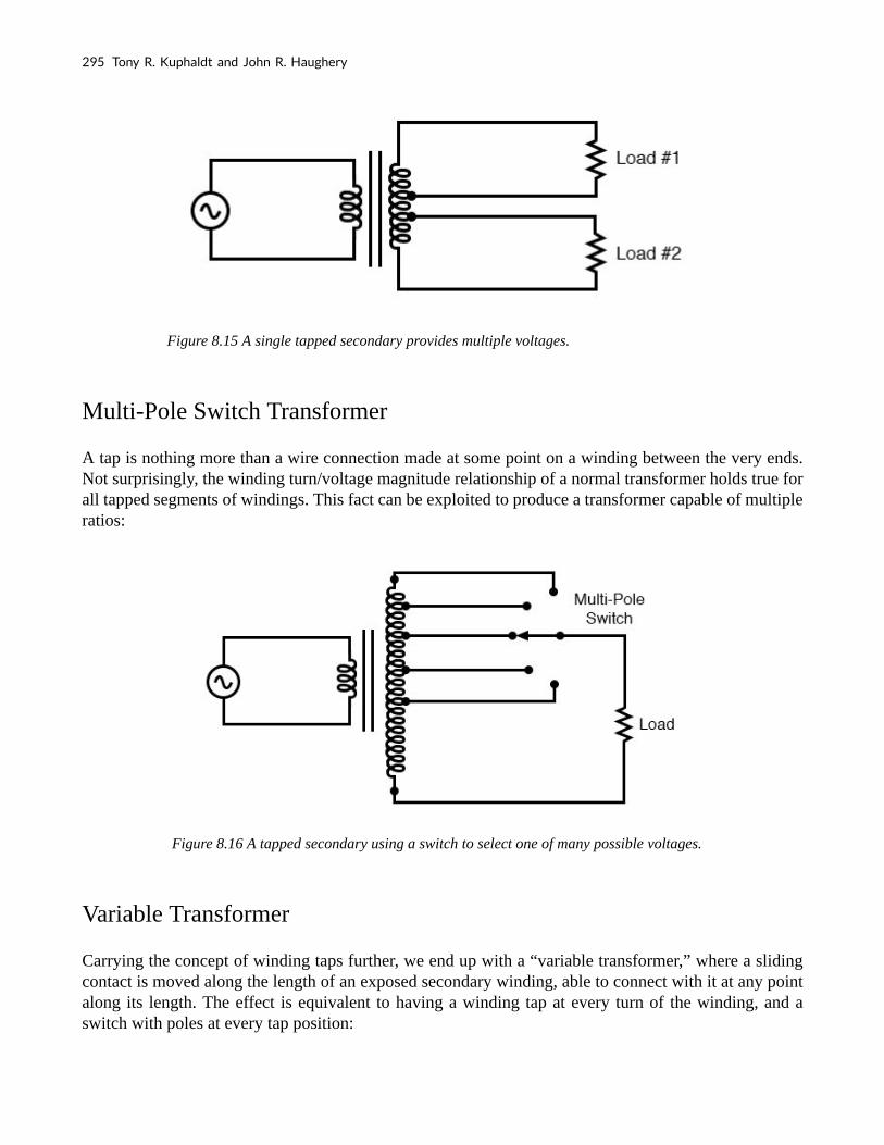
Figure 8.15 A single tapped secondary provides multiple voltages.
Multi-Pole Switch Transformer
A tap is nothing more than a wire connection made at some point on a winding between the very ends. Not surprisingly, the winding turn/voltage magnitude relationship of a normal transformer holds true for all tapped segments of windings. This fact can be exploited to produce a transformer capable of multiple ratios:
Figure 8.16 A tapped secondary using a switch to select one of many possible voltages.
Variable Transformer
Carrying the concept of winding taps further, we end up with a “variable transformer,” where a sliding contact is moved along the length of an exposed secondary winding, able to connect with it at any point along its length. The effect is equivalent to having a winding tap at every turn of the winding, and a switch with poles at every tap position:
295 Tony R. Kuphaldt and John R. Haughery

Figure 8.17 A sliding contact on the secondary continuously varies the secondary voltage.
One consumer application of the variable transformer is in speed controls for model train sets, especially the train sets of the 1950s and 1960s. These transformers were essentially step-down units, the highest voltage obtainable from the secondary winding being substantially less than the primary voltage of 110 to 120 volts AC. The variable-sweep contact provided a simple means of voltage control with little-wasted power, much more efficient than control using a variable resistor!
Moving-slide contacts are too impractical to be used in large industrial power transformer designs, but multi-pole switches and winding taps are common for voltage adjustment. Adjustments need to be made periodically in power systems to accommodate changes in loads over months or years in time, and these switching circuits provide a convenient means. Typically, such “tap switches” are not engineered to handle the full-load current, but must be actuated only when the transformer has been de-energized (no power).
Autotransformer
Seeing as how we can tap any transformer winding to obtain the equivalent of several windings (albeit with loss of electrical isolation between them), it makes sense that it should be possible to forego electrical isolation altogether and build a transformer from a single winding. Indeed this is possible, and the resulting device is called an autotransformer:
Applied Industrial Electricity 296

Figure 8.18 This autotransformer steps the voltage up with a single tapped winding, saving copper, sacrificing isolation.
The autotransformer depicted above performs a voltage step-up function. A step-down autotransformer would look something like the figure below.
Figure 8.19 This autotransformer steps the voltage down with a single copper-saving tapped winding.
Autotransformers find popular use in applications requiring a slight boost or reduction in voltage to a load. The alternative with a normal (isolated) transformer would be to either have just the right primary/secondary winding ratio made for the job or use a step-down configuration with the secondary winding connected in series-aiding (“boosting”) or series-opposing (“bucking”) fashion. Primary, secondary, and load voltages are given to illustrate how this would work.
297 Tony R. Kuphaldt and John R. Haughery

Autotransformer Configurations
First, the “boosting” configuration. In the figure below the secondary coil’s polarity is oriented so that its voltage directly adds to the primary voltage.
Figure 8.20 Ordinary transformer wired as an autotransformer to boost the line voltage.
Next, the “bucking” configuration. In the figure below, the secondary coil’s polarity is oriented so that its voltage directly subtracts from the primary voltage:
Figure 8.21 Ordinary transformer wired as an autotransformer to buck the line voltage down.
The prime advantage of an autotransformer is that the same boosting or bucking function is obtained with only a single winding, making it cheaper and lighter to manufacture than a regular (isolating) transformer having both primary and secondary windings.
Variac Variable Autotransformer
Like regular transformers, autotransformer windings can be tapped to provide variations in ratio. Additionally, they can be made continuously variable with a sliding contact to tap the winding at any
Applied Industrial Electricity 298

point along its length. The latter configuration is popular enough to have earned itself its own name: the Variac. (figure below)
Figure 8.22 A variac is an autotransformer with a sliding tap.
Small variacs for benchtop use are popular pieces of equipment for the electronics experimenter, being able to step household AC voltage down (or sometimes up as well) with a wide, fine range of control by a simple twist of a knob.
Review
• Transformers can be equipped with more than just a single primary and single
secondary winding pair. This allows for multiple step-up and/or step-down ratios in
the same device.
• Transformer windings can also be “tapped:” that is, intersected at many points to
segment a single winding into sections.
• Variable transformers can be made by providing a movable arm that sweeps across
the length of a winding, making contact with the winding at any point along its
length. The winding, of course, has to be bare (no insulation) in the area where the
arm sweeps.
• An autotransformer is a single, tapped inductor coil used to step up or step down
voltage like a transformer, except without providing electrical isolation.
299 Tony R. Kuphaldt and John R. Haughery

• A Variac is a variable autotransformer.
8.5 Three-phase Transformer Circuits
Since three-phase is used so often for power distribution systems, it makes sense that we would need three-phase transformers to be able to step voltages up or down. This is only partially true, as regular single-phase transformers can be ganged together to transform power between two three-phase systems in a variety of configurations, eliminating the requirement for a special three-phase transformer. However, special three-phase transformers are built for those tasks and are able to perform with less material requirement, less size, and less weight than their modular counterparts.
Three-Phase Transformer Windings and Connections
A three-phase transformer is made of three sets of primary and secondary windings, each set wound around one leg of an iron core assembly. Essentially it looks like three single-phase transformers sharing a joined core as in Figure below.
Figure 8.23 Three phase transformer core has three sets of windings.
Those sets of primary and secondary windings will be connected in either Δ or Y configurations to form a complete unit. The various combinations of ways that these windings can be connected together it will be the focus of this section.
Whether the winding sets share a common core assembly or each winding pair is a separate transformer, the winding connection options are the same:
Primary – Secondary
• Y – Y
Applied Industrial Electricity 300

• Y – Δ
• Δ – Y
• Δ – Δ
The reasons for choosing a Y or Δ configuration for transformer winding connections are the same as for any other three-phase application: Y connections provide the opportunity for multiple voltages, while Δ connections enjoy a higher level of reliability (if one winding fails open, the other two can still maintain full line voltages to the load).
Probably the most important aspect of connecting three sets of primary and secondary windings together to form a three-phase transformer bank is paying attention to proper winding phasing (the dots used to denote “polarity” of windings). Remember the proper phase relationships between the phase windings of Δ and Y: (Figure below)
Figure 8.24 (Y) The center point of the “Y” must tie either all the “-” or all the “+” winding points together. (Δ) The winding polarities must stack together in a complementary manner ( + to -).
Getting this phasing correct when the windings aren’t shown in regular Y or Δ configuration can be tricky. Let me illustrate, starting with the figure below.
301 Tony R. Kuphaldt and John R. Haughery
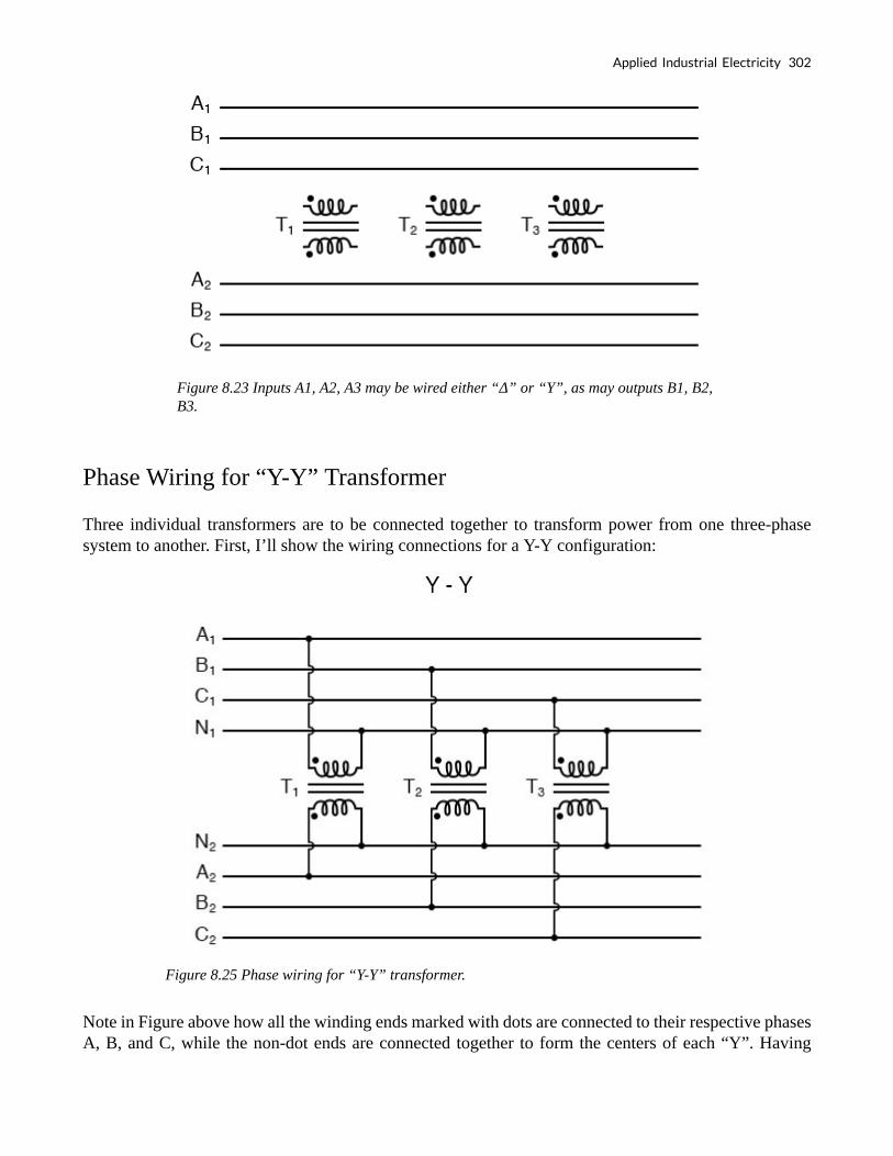
Figure 8.23 Inputs A1, A2, A3 may be wired either “Δ” or “Y”, as may outputs B1, B2, B3.
Phase Wiring for “Y-Y” Transformer
Three individual transformers are to be connected together to transform power from one three-phase system to another. First, I’ll show the wiring connections for a Y-Y configuration:
Figure 8.25 Phase wiring for “Y-Y” transformer.
Note in Figure above how all the winding ends marked with dots are connected to their respective phases A, B, and C, while the non-dot ends are connected together to form the centers of each “Y”. Having
Applied Industrial Electricity 302

both primary and secondary winding sets connected in “Y” formations allows for the use of neutral conductors (N1 and N2) in each power system.
Phase Wiring for “Y-Δ” Transformer
Now, we’ll take a look at a Y-Δ configuration:
Figure 8.26 Phase wiring for “Y-Δ” transformer.
Note how the secondary windings (bottom set, Figure above) are connected in a chain, the “dot” side of one winding connected to the “non-dot” side of the next, forming the Δ loop. At every connection point between pairs of windings, a connection is made to a line of the second power system (A, B, and C).
Phase Wiring for “Δ-Y” Transformer
Now, let’s examine a Δ-Y system in the figure below.
303 Tony R. Kuphaldt and John R. Haughery
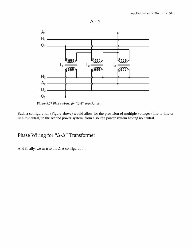
Figure 8.27 Phase wiring for “Δ-Y” transformer.
Such a configuration (Figure above) would allow for the provision of multiple voltages (line-to-line or line-to-neutral) in the second power system, from a source power system having no neutral.
Phase Wiring for “Δ-Δ” Transformer
And finally, we turn to the Δ-Δ configuration:
Applied Industrial Electricity 304

Figure 8.28 Phase wiring for “Δ-Δ” transformer.
When there is no need for a neutral conductor in the secondary power system, Δ-Δ connection schemes (Figure above) are preferred because of the inherent reliability of the Δ configuration.
Phase Wiring for “V” or “open-Δ” Transformer
Considering that a Δ configuration can operate satisfactorily missing one winding, some power system designers choose to create a three-phase transformer bank with only two transformers, representing a Δ-Δ configuration with a missing winding in both the primary and secondary sides:
305 Tony R. Kuphaldt and John R. Haughery
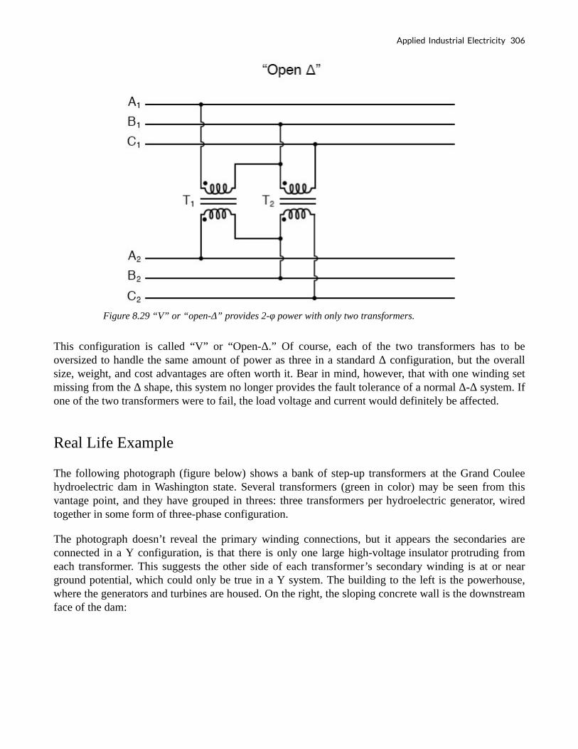
Figure 8.29 “V” or “open-Δ” provides 2-φ power with only two transformers.
This configuration is called “V” or “Open-Δ.” Of course, each of the two transformers has to be oversized to handle the same amount of power as three in a standard Δ configuration, but the overall size, weight, and cost advantages are often worth it. Bear in mind, however, that with one winding set missing from the Δ shape, this system no longer provides the fault tolerance of a normal Δ-Δ system. If one of the two transformers were to fail, the load voltage and current would definitely be affected.
Real Life Example
The following photograph (figure below) shows a bank of step-up transformers at the Grand Coulee hydroelectric dam in Washington state. Several transformers (green in color) may be seen from this vantage point, and they have grouped in threes: three transformers per hydroelectric generator, wired together in some form of three-phase configuration.
The photograph doesn’t reveal the primary winding connections, but it appears the secondaries are connected in a Y configuration, is that there is only one large high-voltage insulator protruding from each transformer. This suggests the other side of each transformer’s secondary winding is at or near ground potential, which could only be true in a Y system. The building to the left is the powerhouse, where the generators and turbines are housed. On the right, the sloping concrete wall is the downstream face of the dam:
Applied Industrial Electricity 306

Figure 8.30 Grand coulee hydroelectric dam
8.6 Practical Considerations – Transformers
Power Capacity As has already been observed, transformers must be well designed in order to achieve acceptable power coupling, tight voltage regulation, and low exciting current distortion. Also, transformers must be designed to carry the expected values of primary and secondary winding current without any trouble. This means the winding conductors must be made of the proper gauge wire to avoid any heating problems.
Ideal Transformer
An ideal transformer would have perfect coupling (no leakage inductance), perfect voltage regulation, perfectly sinusoidal exciting current, no hysteresis or eddy current losses, and wire thick enough to handle any amount of current. Unfortunately, the ideal transformer would have to be infinitely large and heavy to meet these design goals. Thus, in the business of practical transformer design, compromises must be made.
Additionally, winding conductor insulation is a concern where high voltages are encountered, as they often are in step-up and step-down power distribution transformers. Not only do the windings have to
307 Tony R. Kuphaldt and John R. Haughery

be well insulated from the iron core, but each winding has to be sufficiently insulated from the other in order to maintain electrical isolation between windings.
Transformer Ratings
Respecting these limitations, transformers are rated for certain levels of primary and secondary winding voltage and current, though the current rating is usually derived from a volt-amp (VA) rating assigned to the transformer. For example, take a step-down transformer with a primary voltage rating of 120 volts, a secondary voltage rating of 48 volts, and a VA rating of 1 kVA (1000 VA). The maximum winding currents can be determined as such:kVA (1000 VA). The maximum winding currents can be determined as such:
Sometimes windings will bear current ratings in amps, but this is typically seen on small transformers. Large transformers are almost always rated in terms of winding voltage and VA or kVA
Energy Losses
When transformers transfer power, they do so with a minimum of loss. As it was stated earlier, modern power transformer designs typically exceed 95% efficiency. It is good to know where some of this lost power goes, however, and what causes it to be lost.
There is, of course, power loss due to the resistance of the wire windings. Unless superconducting wires are used, there will always be power dissipated in the form of heat through the resistance of current-carrying conductors. Because transformers require such long lengths of wire, this loss can be a significant factor. Increasing the gauge of the winding wire is one way to minimize this loss, but only with substantial increases in cost, size, and weight.
Eddy-Current Loss
Resistive losses aside, the bulk of transformer power loss is due to magnetic effects in the core. Perhaps the most significant of these “core losses” is an eddy-current loss, which is resistive power dissipation
Applied Industrial Electricity 308

due to the passage of induced currents through the iron of the core. Because iron is a conductor of electricity as well as being an excellent “conductor” of magnetic flux, there will be currents induced in the iron just as there are currents induced in the secondary windings from the alternating magnetic field. These induced currents—as described by the perpendicularity clause of Faraday’s Law —tend to circulate through the cross-section of the core perpendicularly to the primary winding turns. Their circular motion gives them their unusual name: like eddies in a stream of water that circulate rather than move in straight lines.
Iron is a fair conductor of electricity, but not as good as the copper or aluminum from which wire windings are typically made. Consequently, these “eddy currents” must overcome significant electrical resistance as they circulate through the core. In overcoming the resistance offered by the iron, they dissipate power in the form of heat. Hence, we have a source of inefficiency in the transformer that is difficult to eliminate.
Induction Heating
This phenomenon is so pronounced that it is often exploited as a means of heating ferrous (iron-containing) materials. The photograph below shows an “induction heating” unit raising the temperature of a large pipe section. Loops of wire covered by high-temperature insulation encircle the pipe’s circumference, inducing eddy currents within the pipe wall by electromagnetic induction. In order to maximize the eddy current effect, high-frequency alternating current is used rather than power line frequency (60 Hz). The box units at the right of the picture produce the high-frequency AC and control the amount of current in the wires to stabilize the pipe temperature at a pre-determined “set-point.”
Figure 8.31 Induction heating: Primary insulated winding induces current into lossy iron pipe (secondary).
309 Tony R. Kuphaldt and John R. Haughery

Mitigating Eddy Currents
The main strategy in mitigating these wasteful eddy currents in transformer cores is to form the iron core in sheets, each sheet covered with an insulating varnish so that the core is divided up into thin slices. The result is very little width in the core for eddy currents to circulate in:
Figure 8.32 Dividing the iron core into thin insulated laminations minimizes eddy current loss.
Laminated cores like the one shown here are standard in almost all low-frequency transformers. Recall from the photograph of the transformer cut in half that the iron core was composed of many thin sheets rather than one solid piece. Eddy current losses increase with frequency, so transformers designed to run on higher-frequency power (such as 400 Hz, used in many military and aircraft applications) must use thinner laminations to keep the losses down to a respectable minimum. This has the undesirable effect of increasing the manufacturing cost of the transformer.
Another, similar technique for minimizing eddy current losses which work better for high-frequency applications is to make the core out of iron powder instead of thin iron sheets. Like the lamination sheets, these granules of iron are individually coated in an electrically insulating material, which makes the core nonconductive except for within the width of each granule. Powdered iron cores are often found in transformers handling radio-frequency currents.
Magnetic Hysteresis
Another “core loss” is that of magnetic hysteresis. All ferromagnetic materials tend to retain some degree of magnetization after exposure to an external magnetic field. This tendency to stay magnetized is called “hysteresis,” and it takes a certain investment in energy to overcome this opposition to change every time the magnetic field produced by the primary winding changes polarity (twice per AC cycle).
This type of loss can be mitigated through good core material selection (choosing a core alloy with low
Applied Industrial Electricity 310

hysteresis, as evidenced by a “thin” B/H hysteresis curve), and designing the core for minimum flux density (large cross-sectional area).
Skin Effect at High Frequencies
Transformer energy losses tend to worsen with increasing frequency. The skin effect within winding conductors reduces the available cross-sectional area for electric charge flow, thereby increasing effective resistance as the frequency goes up and creating more power lost through resistive dissipation. Magnetic core losses are also exaggerated with higher frequencies, eddy currents, and hysteresis effects becoming more severe. For this reason, transformers of significant size are designed to operate efficiently in a limited range of frequencies.
In most power distribution systems where the line frequency is very stable, one would think excessive frequency would never pose a problem. Unfortunately, it does, in the form of harmonics created by nonlinear loads.
As we’ve seen in earlier chapters, nonsinusoidal waveforms are equivalent to additive series of multiple sinusoidal waveforms at different amplitudes and frequencies. In power systems, these other frequencies are whole-number multiples of the fundamental (line) frequency, meaning that they will always be higher, not lower, than the design frequency of the transformer. In significant measure, they can cause severe transformer overheating. Power transformers can be engineered to handle certain levels of power system harmonics, and this capability is sometimes denoted with a “K factor” rating.
Stray Capacitance and Inductance
Aside from power ratings and power losses, transformers often harbor other undesirable limitations that circuit designers must be made aware of. Like their simpler counterparts—inductors—transformers exhibit capacitance due to the insulation dielectric between conductors: from winding to winding, turn to turn (in a single winding), and winding to the core.
Transformer Resonance Frequency
Usually, this capacitance is of no concern in a power application, but small signal applications (especially those of high frequency) may not tolerate this quirk well. Also, the effect of having capacitance along with the windings’ designed inductance gives transformers the ability to resonate at a particular frequency, definitely a design concern in signal applications where the applied frequency may reach this point (usually the resonant frequency of a power transformer is well beyond the frequency of the AC power it was designed to operate on).
311 Tony R. Kuphaldt and John R. Haughery

Flux Containment
Flux containment (making sure a transformer’s magnetic flux doesn’t escape so as to interfere with another device, and making sure other devices’ magnetic flux is shielded from the transformer core) is another concern shared both by inductors and transformers.
Leakage Inductance
Closely related to the issue of flux containment is leakage inductance. Because leakage inductance is equivalent to an inductance connected in series with the transformer’s winding, it manifests itself as a series impedance with the load. Thus, the more current drawn by the load, the less voltage available at the secondary winding terminals. Usually, good voltage regulation is desired in transformer design, but there are exceptional applications. As was stated before, discharge lighting circuits require a step-up transformer with “loose” (poor) voltage regulation to ensure reduced voltage after the establishment of an arc through the lamp. One way to meet this design criterion is to engineer the transformer with flux leakage paths for magnetic flux to bypass the secondary winding(s). The resulting leakage flux will produce leakage inductance, which will, in turn, produce the poor regulation needed for discharge lighting.
Core Saturation
Transformers are also constrained in their performance by the magnetic flux limitations of the core. For ferromagnetic core transformers, we must be mindful of the saturation limits of the core. Remember that ferromagnetic materials cannot support infinite magnetic flux densities: they tend to “saturate” at a certain level (dictated by the material and core dimensions), meaning that further increases in magnetic field force (mmf) do not result in proportional increases in magnetic field flux (Φ).
When a transformer’s primary winding is overloaded from excessive applied voltage, the core flux may reach saturation levels during peak moments of the AC sine wave cycle. If this happens, the voltage induced in the secondary winding will no longer match the wave-shape as the voltage powering the primary coil. In other words, the overloaded transformer will distort the waveshape from primary to secondary windings, creating harmonics in the secondary winding’s output. As we discussed before, harmonic content in AC power systems typically causes problems.
Peaking Transformers
Special transformers known as peaking transformers exploit this principle to produce brief voltage pulses near the peaks of the source voltage waveform. The core is designed to saturate quickly and sharply, at voltage levels well below peak. This results in a severely cropped sine-wave flux waveform, and secondary voltage pulses only when the flux is changing (below saturation levels):
Applied Industrial Electricity 312

Figure 8.33 Voltage and flux waveforms for a peaking transformer.
Operation at Frequencies Lower than Normal
Another cause of abnormal transformer core saturation is operation at frequencies lower than normal. For example, if a power transformer designed to operate at 60 Hz is forced to operate at 50 Hz instead, the flux must reach greater peak levels than before in order to produce the same opposing voltage needed to balance against the source voltage. This is true even if the source voltage is the same as before.
Figure 8.34 Magnetic flux is higher in a transformer core driven by 50 Hz as compared to 60 Hz for the same voltage.
Since instantaneous winding voltage is proportional to the instantaneous magnetic flux’s rate of change in a transformer, a voltage waveform reaching the same peak value, but taking a longer amount of time to complete each half-cycle, demands that the flux maintain the same rate of change as before, but for longer periods of time. Thus, if the flux has to climb at the same rate as before, but for longer periods of time, it will climb to a greater peak value.
313 Tony R. Kuphaldt and John R. Haughery

Mathematically, this is another example of calculus in action. Because the voltage is proportional to the flux’s rate-of-change, we say that the voltage waveform is the derivative of the flux waveform, “derivative” being that calculus operation defining one mathematical function (waveform) in terms of the rate-of-change of another. If we take the opposite perspective, though, and relate the original waveform to its derivative, we may call the original waveform the integral of the derivative waveform. In this case, the voltage waveform is the derivative of the flux waveform, and the flux waveform is the integral of the voltage waveform.
The integral of any mathematical function is proportional to the area accumulated underneath the curve of that function. Since each half-cycle of the 50 Hz waveform accumulates more area between it and the zero line of the graph than the 60 Hz waveform will—and we know that the magnetic flux is the integral of the voltage—the flux will attain higher values in the Figure below.
Figure 8.35 Flux changing at the same rate rises to a higher level at 50 Hz than at 60 Hz.
Yet another cause of transformer saturation is the presence of DC current in the primary winding. Any amount of DC voltage dropped across the primary winding of a transformer will cause an additional magnetic flux in the core. This additional flux “bias” or “offset” will push the alternating flux waveform closer to saturation in one half-cycle than the other.
Applied Industrial Electricity 314

Figure 8.36 DC in primary, shifts the waveform peaks toward the upper saturation limit.
For most transformers, core saturation is a very undesirable effect, and it is avoided through good design: engineering the windings and core so that magnetic flux densities remain well below the saturation levels. This ensures that the relationship between mmf and Φ is more linear throughout the flux cycle, which is good because it makes for less distortion in the magnetization current waveform. Also, engineering the core for low flux densities provides a safe margin between the normal flux peaks and the core saturation limits to accommodate occasional, abnormal conditions such as frequency variation and DC offset.
Inrush Current
When a transformer is initially connected to a source of AC voltage, there may be a substantial surge of current through the primary winding called inrush current. This is analogous to the inrush current exhibited by an electric motor that is started up by sudden connection to a power source, although transformer inrush is caused by a different phenomenon.
We know that the rate of change of instantaneous flux in a transformer core is proportional to the instantaneous voltage drop across the primary winding. Or, as stated before, the voltage waveform is the derivative of the flux waveform, and the flux waveform is the integral of the voltage waveform. In a continuously-operating transformer, these two waveforms are phase-shifted by 90°. Since flux (Φ) is proportional to the magnetomotive force (mmf) in the core, and the mmf is proportional to winding current, the current waveform will be in-phase with the flux waveform, and both will be lagging the voltage waveform by 90°:
315 Tony R. Kuphaldt and John R. Haughery

Figure 8.37 Continuous steady-state operation: Magnetic flux, like current, lags applied voltage by 90°.
Let us suppose that the primary winding of a transformer is suddenly connected to an AC voltage source at the exact moment in time when the instantaneous voltage is at its positive peak value. In order for the transformer to create an opposing voltage drop to balance against this applied source voltage, a magnetic flux of rapidly increasing value must be generated. The result is that winding current increases rapidly, but actually no more rapidly than under normal conditions:
Figure 8.38 Connecting transformer to line at AC volt peak: Flux increases rapidly from zero, same as steady-state operation.
Both core flux and coil current start from zero and build up to the same peak values experienced during continuous operation. Thus, there is no “surge” or “inrush” or current in this scenario.
Alternatively, let us consider what happens if the transformer’s connection to the AC voltage source occurs at the exact moment in time when the instantaneous voltage is at zero. During continuous operation (when the transformer has been powered for quite some time), this is the point in time where both flux and winding current are at their negative peaks, experiencing zero rate-of-change (dΦ/dt = 0 and di/dt = 0). As the voltage builds to its positive peak, the flux and current waveforms build to their
Applied Industrial Electricity 316

maximum positive rates-of-change, and on upward to their positive peaks as the voltage descends to a level of zero:
Figure 8.39 Starting at e=0 V is not the same as running continuously in Figure above. These expected waveforms are incorrect– Φ and i should start at zero.
A significant difference exists, however, between continuous-mode operation and the sudden starting condition assumed in this scenario: during continuous operation, the flux and current levels were at their negative peaks when voltage was at its zero points; in a transformer that has been sitting idle, however, both magnetic flux and winding current should start at zero.
When the magnetic flux increases in response to a rising voltage, it will increase from zero upward, not from a previously negative (magnetized) condition as we would normally have in a transformer that’s been powered for a while. Thus, in a transformer that’s just “starting,” the flux will reach approximately twice its normal peak magnitude as it “integrates” the area under the voltage waveform’s first half-cycle:
317 Tony R. Kuphaldt and John R. Haughery

Figure 8.40 Starting at e=0 V, Φ starts at initial condition Φ=0, increasing to twice the normal value, assuming it doesn’t saturate the core.
Starting at e=0 V, Φ starts at initial condition Φ=0, increasing to twice the normal value, assuming it doesn’t saturate the core.
In an ideal transformer, the magnetizing current would rise to approximately twice its normal peak value as well, generating the necessary mmf to create this higher-than-normal flux. However, most transformers aren’t designed with enough of a margin between normal flux peaks and the saturation limits to avoid saturating in a condition like this, and so the core will almost certainly saturate during this first half-cycle of voltage. During saturation, disproportionate amounts of mmf are needed to generate magnetic flux. This means that winding current, which creates the mmf to cause a flux in the core, will disproportionately rise to a value easily exceeding twice its normal peak:
Applied Industrial Electricity 318

Figure 8.41 Starting at e=0 V, Current also increases to twice the normal value for an unsaturated core, or considerably higher in the (designed for) case of saturation.
This is the mechanism causing inrush current in a transformer’s primary winding when connected to an AC voltage source. As you can see, the magnitude of the inrush current strongly depends on the exact time that electrical connection to the source is made. If the transformer happens to have some residual magnetism in its core at the moment of connection to the source, the inrush could be even more severe. Because of this, transformer overcurrent protection devices are usually of the “slow-acting” variety, so as to tolerate current surges such as this without opening the circuit.
Heat and Noise
In addition to unwanted electrical effects, transformers may also exhibit undesirable physical effects, the most notable being the production of heat and noise. Noise is primarily a nuisance effect, but heat is a potentially serious problem because winding insulation will be damaged if allowed to overheat. Heating may be minimized by good design, ensuring that the core does not approach saturation levels, that eddy currents are minimized, and that the windings are not overloaded or operated too close to maximum ampacity.
Large power transformers have their core and windings submerged in an oil bath to transfer heat and muffle noise, and also to displace moisture which would otherwise compromise the integrity of the winding insulation. Heat-dissipating “radiator” tubes on the outside of the transformer case provide a convective oil flow path to transfer heat from the transformer’s core to ambient air:
319 Tony R. Kuphaldt and John R. Haughery

Figure 8.42 Large power transformers are submerged in heat dissipating insulating oil.
Oil-less, or “dry,” transformers are often rated in terms of maximum operating temperature “rise” (temperature increase beyond ambient) according to a letter-class system: A, B, F, or H. These letter codes are arranged in order of lowest heat tolerance to highest:
• Class A: No more than 55° Celsius winding temperature rise, at 40° Celsius (maximum) ambient air temperature.
• Class B: No more than 80° Celsius winding temperature rise, at 40° Celsius (maximum)ambient air temperature.
• Class F: No more than 115° Celsius winding temperature rise, at 40° Celsius (maximum)ambient air temperature.
• Class H: No more than 150° Celsius winding temperature rise, at 40° Celsius (maximum)ambient air temperature.
Audible noise is an effect primarily originating from the phenomenon of magnetostriction: the slight change of length exhibited by a ferromagnetic object when magnetized. The familiar “hum” heard around large power transformers is the sound of the iron core expanding and contracting at 120 Hz (twice the system frequency, which is 60 Hz in the United States)—one cycle of core contraction and expansion for every peak of the magnetic flux waveform—plus noise created by mechanical forces between primary and secondary windings. Again, maintaining low magnetic flux levels in the core is the
Applied Industrial Electricity 320

key to minimizing this effect, which explains why ferroresonant transformers—which must operate in saturation for a large portion of the current waveform—operate both hot and noisy.
Losses due to Winding Magnetic Forces
Another noise-producing phenomenon in power transformers is the physical reaction force between primary and secondary windings when heavily loaded. If the secondary winding is open-circuited, there will be no current through it, and consequently, no magneto-motive force (mmf) produced by it. However, when the secondary is “loaded” (currently supplied to a load), the winding generates an mmf, which becomes counteracted by a “reflected” mmf in the primary winding to prevent core flux levels from changing. These opposing mmf’s generated between primary and secondary windings as a result of secondary (load) current produce a repulsive, physical force between the windings which will tend to make them vibrate. Transformer designers have to consider these physical forces in the construction of the winding coils, to ensure there is adequate mechanical support to handle the stresses. Under heavy load (high current) conditions, though, these stresses may be great enough to cause audible noise to emanate from the transformer.
Review
• Power transformers are limited in the amount of power they can transfer from
primary to secondary winding(s). Large units are typically rated in VA (volt-amps)
or kVA (kilo volt-amps).
• Resistance in transformer windings contributes to inefficiency, as current will
dissipate heat, wasting energy.
• Magnetic effects in a transformer’s iron core also contribute to inefficiency. Among
the effects are eddy currents (circulating induction currents in the iron core)
and hysteresis (power lost due to overcoming the tendency of iron to magnetize in a
particular direction).
• Increased frequency results in increased power losses within a power transformer.
The presence of harmonics in a power system is a source of frequencies
significantly higher than normal, which may cause overheating in large
transformers.
321 Tony R. Kuphaldt and John R. Haughery

• Both transformers and inductors harbor certain unavoidable amounts of capacitance
due to wire insulation (dielectric) separating winding turns from the iron core and
from each other. This capacitance can be significant enough to give the transformer
a natural resonant frequency, which can be problematic in signal applications.
• Leakage inductance is caused by magnetic flux not being 100% coupled between
windings in a transformer. Any flux not involved with transferring energy from one
winding to another will store and release energy, which is how (self-) inductance
works. Leakage inductance tends to worsen a transformer’s voltage regulation
(secondary voltage “sags” more for a given amount of load current).
• Magnetic saturation of a transformer core may be caused by excessive primary
voltage, operation at too low of a frequency, and/or by the presence of a DC current
in any of the windings. Saturation may be minimized or avoided by conservative
design, which provides an adequate margin of safety between peak magnetic flux
density values and the saturation limits of the core.
• Transformers often experience significant inrush currents when initially connected
to an AC voltage source. Inrush current is most severe when the connection to the
AC source is made at the moment instantaneous source voltage is zero.
• Noise is a common phenomenon exhibited by transformers—especially power
transformers—and is primarily caused by magnetostriction of the core. Physical
forces causing winding vibration may also generate noise under conditions of heavy
(high current) secondary winding load.
Applied Industrial Electricity 322

9. INDUSTRIAL CONTROLS
9.1 Switch Types
Though it may seem strange to cover the elementary topic of electrical switches at such a late stage in this book series, I do so because the chapters that follow explore an older realm of digital technology based on mechanical switch contacts rather than solid-state gate circuits, and a thorough understanding of switch types is necessary for the undertaking. Learning the function of switch-based circuits at the same time that you learn about solid-state logic gates makes both topics easier to grasp, and sets the stage for an enhanced learning experience in Boolean algebra, the mathematics behind digital logic circuits.
What is an Electrical Switch?
An electrical switch is any device used to interrupt the flow of electrons in a circuit. Switches are essentially binary devices: they are either completely on (“closed”) or completely off (“open”). There are many different types of switches, and we will explore some of these types in this chapter.
Learn the Different Types of Switches
The simplest type of switch is one where two electrical conductors are brought in contact with each other by the motion of an actuating mechanism. Other switches are more complex, containing electronic circuits able to turn on or off depending on some physical stimulus (such as light or magnetic field) sensed. In any case, the final output of any switch will be (at least) a pair of wire-connection terminals that will either be connected together by the switch’s internal contact mechanism (“closed”), or not connected together (“open”). Any switch designed to be operated by a person is generally called a hand switch, and they are manufactured in several varieties:
Toggle Switches
Figure 9.1 Toggle switch
323

Toggle switches are actuated by a lever angled in one of two or more positions. The common light switch used in household wiring is an example of a toggle switch. Most toggle switches will come to rest in any of their lever positions, while others have an internal spring mechanism returning the lever to a certain normal position, allowing for what is called “momentary” operation.
Push button Switches
Figure 9.2 Push button Switch
Push button switches are two-position devices actuated with a button that is pressed and released. Most push button switches have an internal spring mechanism returning the button to its “out,” or “unpressed,” position, for momentary operation. Some push button switches will latch alternately on or off with every push of the button. Other push button switches will stay in their “in,” or “pressed,” position until the button is pulled back out. This last type of pushbutton switches usually have a mushroom-shaped button for easy push-pull action.
Selector Switches
Figure 9.3 Selector Switch
Applied Industrial Electricity 324

Selector switches are actuated with a rotary knob or lever of some sort to select one of two or more positions. Like the toggle switch, selector switches can either rest in any of their positions or contain spring-return mechanisms for momentary operation.
Joystick Switches
Figure 9.4 Joystick switch
A joystick switch is actuated by a lever free to move in more than one axis of motion. One or more of several switch contact mechanisms are actuated depending on which way the lever is pushed, and sometimes by how far it is pushed. The circle-and-dot notation on the switch symbol represents the direction of joystick lever motion required to actuate the contact. Joystick hand switches are commonly used for crane and robot control.
Some switches are specifically designed to be operated by the motion of a machine rather than by the hand of a human operator. These motion-operated switches are commonly called limit switches, because they are often used to limit the motion of a machine by turning off the actuating power to a component if it moves too far.
As with hand switches, limit switches come in several varieties:
325 Tony R. Kuphaldt and John R. Haughery
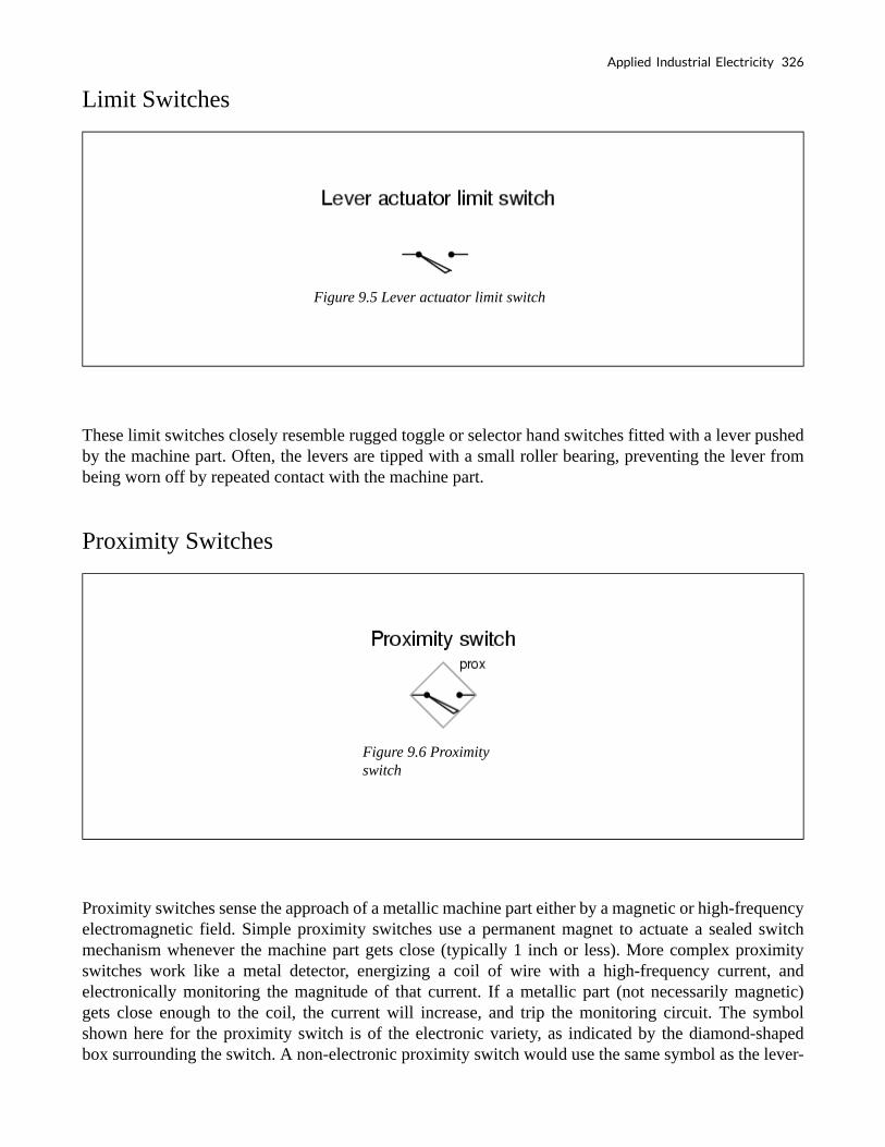
Limit Switches
Figure 9.5 Lever actuator limit switch
These limit switches closely resemble rugged toggle or selector hand switches fitted with a lever pushed by the machine part. Often, the levers are tipped with a small roller bearing, preventing the lever from being worn off by repeated contact with the machine part.
Proximity Switches
Figure 9.6 Proximity switch
Proximity switches sense the approach of a metallic machine part either by a magnetic or high-frequency electromagnetic field. Simple proximity switches use a permanent magnet to actuate a sealed switch mechanism whenever the machine part gets close (typically 1 inch or less). More complex proximity switches work like a metal detector, energizing a coil of wire with a high-frequency current, and electronically monitoring the magnitude of that current. If a metallic part (not necessarily magnetic) gets close enough to the coil, the current will increase, and trip the monitoring circuit. The symbol shown here for the proximity switch is of the electronic variety, as indicated by the diamond-shaped box surrounding the switch. A non-electronic proximity switch would use the same symbol as the lever-
Applied Industrial Electricity 326

actuated limit switch. Another form of proximity switch is the optical switch, comprised of a light source and photocell. Machine position is detected by either the interruption or reflection of a light beam. Optical switches are also useful in safety applications, where beams of light can be used to detect personnel entry into a dangerous area.
The Different Types of Process Switches
In many industrial processes, it is necessary to monitor various physical quantities with switches. Such switches can be used to sound alarms, indicating that a process variable has exceeded normal parameters, or they can be used to shut down processes or equipment if those variables have reached dangerous or destructive levels. There are many different types of process switches.
Speed Switches
Figure 9.7 Speed switch.
These switches sense the rotary speed of a shaft either by a centrifugal weight mechanism mounted on the shaft, or by some kind of non-contact detection of shaft motion such as optical or magnetic.
327 Tony R. Kuphaldt and John R. Haughery

Pressure Switches
Figure 9.8 Pressure switch
Gas or liquid pressure can be used to actuate a switch mechanism if that pressure is applied to a piston, diaphragm, or bellows, which converts pressure to mechanical force.
Temperature Switches
Figure 9.9 Temperature switch
An inexpensive temperature-sensing mechanism is the “bimetallic strip:” a thin strip of two metals, joined back-to-back, each metal having a different rate of thermal expansion. When the strip heats or cools, differing rates of thermal expansion between the two metals causes it to bend. The bending of the strip can then be used to actuate a switch contact mechanism. Other temperature switches use a brass bulb filled with either a liquid or gas, with a tiny tube connecting the bulb to a pressure-sensing switch. As the bulb is heated, the gas or liquid expands, generating a pressure increase which then actuates the switch mechanism.
Applied Industrial Electricity 328

Liquid Level Switch
Figure 9.10 Liquid level switch.
A floating object can be used to actuate a switch mechanism when the liquid level in an tank rises past a certain point. If the liquid is electrically conductive, the liquid itself can be used as a conductor to bridge between two metal probes inserted into the tank at the required depth. The conductivity technique is usually implemented with a special design of relay triggered by a small amount of current through the conductive liquid. In most cases it is impractical and dangerous to switch the full load current of the circuit through a liquid. Level switches can also be designed to detect the level of solid materials such as wood chips, grain, coal, or animal feed in a storage silo, bin, or hopper. A common design for this application is a small paddle wheel, inserted into the bin at the desired height, which is slowly turned by a small electric motor. When the solid material fills the bin to that height, the material prevents the paddle wheel from turning. The torque response of the small motor than trips the switch mechanism. Another design uses a “tuning fork” shaped metal prong, inserted into the bin from the outside at the desired height. The fork is vibrated at its resonant frequency by an electronic circuit and magnet/electromagnet coil assembly. When the bin fills to that height, the solid material dampens the vibration of the fork, the change in vibration amplitude and/or frequency detected by the electronic circuit.
329 Tony R. Kuphaldt and John R. Haughery

Liquid Flow Switch
Figure 9.11 Liquid flow switch.
Inserted into a pipe, a flow switch will detect any gas or liquid flow rate in excess of a certain threshold, usually with a small paddle or vane which is pushed by the flow. Other flow switches are constructed as differential pressure switches, measuring the pressure drop across a restriction built into the pipe.
Nuclear Level Switch
Figure 9.12 Nuclear level switch.
Another type of level switch, suitable for liquid or solid material detection, is the nuclear switch. Composed of a radioactive source material and a radiation detector, the two are mounted across the diameter of a storage vessel for either solid or liquid material. Any height of material beyond the level
Applied Industrial Electricity 330

of the source/detector arrangement will attenuate the strength of radiation reaching the detector. This decrease in radiation at the detector can be used to trigger a relay mechanism to provide a switch contact for measurement, alarm point, or even control of the vessel level.
Bource and detector are outside of the vessel, with no intrusion at all except the radiation flux itself. The radioactive sources used are fairly weak and pose no immediate health threat to operations or maintenance personnel.
All Switches Have Multiple Applications
As usual, there is more than one way to implement a switch to monitor a physical process or serve as an operator control. There is usually no single “perfect” switch for any application, although some obviously exhibit certain advantages over others. Switches must be intelligently matched to the task for efficient and reliable operation.
Review
• A switch is an electrical device, usually electromechanical, used to control
continuity between two points.
• Hand switches are actuated by human touch.
• Limit switches are actuated by machine motion.
• Process switches are actuated by changes in some physical process (temperature,
level, flow, etc.).
9.2 Switch Contact Design
A switch can be constructed with any mechanism bringing two conductors into contact with each other in a controlled manner. This can be as simple as allowing two copper wires to touch each other by the motion of a lever, or by directly pushing two metal strips into contact. However, a good switch design must be rugged and reliable, and avoid presenting the operator with the possibility of electric shock. Therefore, industrial switch designs are rarely this crude. The conductive parts in a switch used to make and break the electrical connection are called contacts. Contacts are typically made of silver or silver-cadmium alloy, whose conductive properties are not significantly compromised by surface corrosion or oxidation. Gold contacts exhibit the best corrosion resistance, but are limited in current-carrying capacity
331 Tony R. Kuphaldt and John R. Haughery

and may “cold weld” if brought together with high mechanical force. Whatever the choice of metal, the switch contacts are guided by a mechanism ensuring square and even contact, for maximum reliability and minimum resistance. Contacts such as these can be constructed to handle extremely large amounts of electric current, up to thousands of amps in some cases. The limiting factors for switch contact ampacity are as follows:
• Heat generated by current through metal contacts (while closed).
• Sparking caused when contacts are opened or closed.
• The voltage across open switch contacts (potential of current jumping across the gap).
One major disadvantage of standard switch contacts is the exposure of the contacts to the surrounding atmosphere. In a nice, clean, control-room environment, this is generally not a problem. However, most industrial environments are not this benign. The presence of corrosive chemicals in the air can cause contacts to deteriorate and fail prematurely. Even more troublesome is the possibility of regular contact sparking causing flammable or explosive chemicals to ignite. When such environmental concerns exist, other types of contacts can be considered for small switches. These other types of contacts are sealed from contact with the outside air, and therefore do not suffer the same exposure problems that standard contacts do. A common type of sealed-contact switch is the mercury switch. Mercury is a metallic element, liquid at room temperature. Being a metal, it possesses excellent conductive properties. Being a liquid, it can be brought into contact with metal probes (to close a circuit) inside of a sealed chamber simply by tilting the chamber so that the probes are on the bottom. Many industrial switches use small glass tubes containing mercury which are tilted one way to close the contact, and tilted another way to open. Aside from the problems of tube breakage and spilling mercury (which is a toxic material), and susceptibility to vibration, these devices are an excellent alternative to open-air switch contacts wherever environmental exposure problems are a concern. Here, a mercury switch (often called a tilt switch) is shown in the open position, where the mercury is out of contact with the two metal contacts at the other end of the glass bulb:
Applied Industrial Electricity 332

Figure 9.13
Figure 9.14
Here, the same switch is shown in the closed position. Gravity now holds the liquid mercury in contact
333 Tony R. Kuphaldt and John R. Haughery
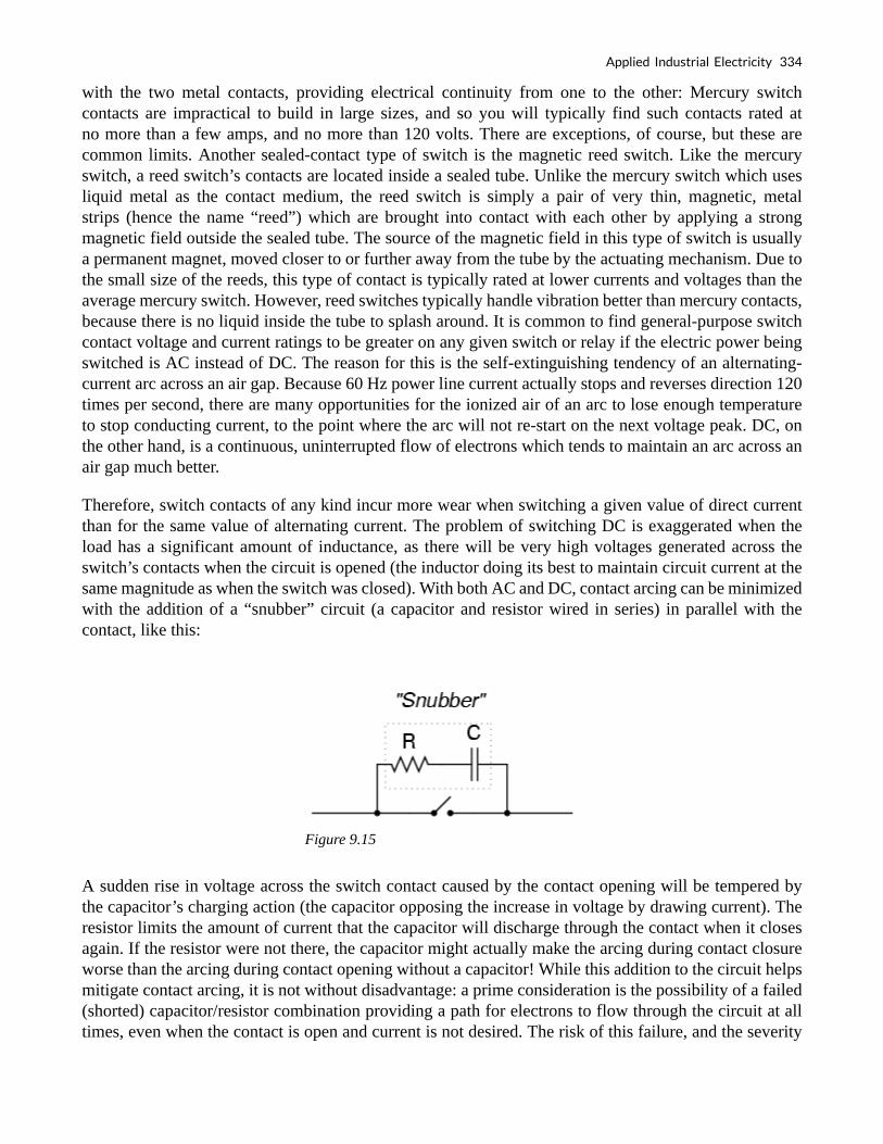
with the two metal contacts, providing electrical continuity from one to the other: Mercury switch contacts are impractical to build in large sizes, and so you will typically find such contacts rated at no more than a few amps, and no more than 120 volts. There are exceptions, of course, but these are common limits. Another sealed-contact type of switch is the magnetic reed switch. Like the mercury switch, a reed switch’s contacts are located inside a sealed tube. Unlike the mercury switch which uses liquid metal as the contact medium, the reed switch is simply a pair of very thin, magnetic, metal strips (hence the name “reed”) which are brought into contact with each other by applying a strong magnetic field outside the sealed tube. The source of the magnetic field in this type of switch is usually a permanent magnet, moved closer to or further away from the tube by the actuating mechanism. Due to the small size of the reeds, this type of contact is typically rated at lower currents and voltages than the average mercury switch. However, reed switches typically handle vibration better than mercury contacts, because there is no liquid inside the tube to splash around. It is common to find general-purpose switch contact voltage and current ratings to be greater on any given switch or relay if the electric power being switched is AC instead of DC. The reason for this is the self-extinguishing tendency of an alternating-current arc across an air gap. Because 60 Hz power line current actually stops and reverses direction 120 times per second, there are many opportunities for the ionized air of an arc to lose enough temperature to stop conducting current, to the point where the arc will not re-start on the next voltage peak. DC, on the other hand, is a continuous, uninterrupted flow of electrons which tends to maintain an arc across an air gap much better.
Therefore, switch contacts of any kind incur more wear when switching a given value of direct current than for the same value of alternating current. The problem of switching DC is exaggerated when the load has a significant amount of inductance, as there will be very high voltages generated across the switch’s contacts when the circuit is opened (the inductor doing its best to maintain circuit current at the same magnitude as when the switch was closed). With both AC and DC, contact arcing can be minimized with the addition of a “snubber” circuit (a capacitor and resistor wired in series) in parallel with the contact, like this:
Figure 9.15
A sudden rise in voltage across the switch contact caused by the contact opening will be tempered by the capacitor’s charging action (the capacitor opposing the increase in voltage by drawing current). The resistor limits the amount of current that the capacitor will discharge through the contact when it closes again. If the resistor were not there, the capacitor might actually make the arcing during contact closure worse than the arcing during contact opening without a capacitor! While this addition to the circuit helps mitigate contact arcing, it is not without disadvantage: a prime consideration is the possibility of a failed (shorted) capacitor/resistor combination providing a path for electrons to flow through the circuit at all times, even when the contact is open and current is not desired. The risk of this failure, and the severity
Applied Industrial Electricity 334

of the resulting consequences must be considered against the increased contact wear (and inevitable contact failure) without the snubber circuit. The use of snubbers in DC switch circuits is nothing new: automobile manufacturers have been doing this for years on engine ignition systems, minimizing the arcing across the switch contact “points” in the distributor with a small capacitor called a condenser. As any mechanic can tell you, the service life of the distributor’s “points” is directly related to how well the condenser is functioning. With all this discussion concerning the reduction of switch contact arcing, one might be led to think that less current is always better for a mechanical switch. This, however, is not necessarily so. It has been found that a small amount of periodic arcing can actually be good for the switch contacts, because it keeps the contact faces free from small amounts of dirt and corrosion. If a mechanical switch contact is operated with too little current, the contacts will tend to accumulate excessive resistance and may fail prematurely! This minimum amount of electric current necessary to keep a mechanical switch contact in good health is called the wetting current. Normally, a switch’s wetting current rating is far below its maximum current rating, and well below its normal operating current load in a properly designed system. However, there are applications where a mechanical switch contact may be required to routinely handle currents below normal wetting current limits (for instance, if a mechanical selector switch needs to open or close a digital logic or analog electronic circuit where the current value is extremely small). In these applications, is it highly recommended that gold-plated switch contacts be specified. Gold is a “noble” metal and does not corrode as other metals will. Such contacts have extremely low wetting current requirements as a result. Normal silver or copper alloy contacts will not provide reliable operation if used in such low-current service!
Review
• The parts of a switch responsible for making and breaking electrical continuity are
called the “contacts.” Usually made of corrosion-resistant metal alloy, contacts are
made to touch each other by a mechanism which helps maintain proper alignment
and spacing.
• Mercury switches use a slug of liquid mercury metal as a moving contact. Sealed in
a glass tube, the mercury contact’s spark is sealed from the outside environment,
making this type of switch ideally suited for atmospheres potentially harboring
explosive vapors.
• Reed switches are another type of sealed-contact device, contact being made by two
thin metal “reeds” inside a glass tube, brought together by the influence of an
external magnetic field.
• Switch contacts suffer greater duress switching DC than AC. This is primarily due
335 Tony R. Kuphaldt and John R. Haughery

to the self-extinguishing nature of an AC arc.
• A resistor-capacitor network called a “snubber” can be connected in parallel with a
switch contact to reduce contact arcing.
• Wetting current is the minimum amount of electric current necessary for a switch
contact to carry in order for it to be self-cleaning. Normally this value is far below
the switch’s maximum current rating.
9.3 Contact “Normal” State and Make/Break Sequence
Any kind of switch contact can be designed so that the contacts “close” (establish continuity) when actuated, or “open” (interrupt continuity) when actuated. For switches that have a spring-return mechanism in them, the direction that the spring returns it to with no applied force is called the normal position. Therefore, contacts that are open in this position are called normally open and contacts that are closed in this position are called normally closed. For process switches, the normal position, or state, is that which the switch is in when there is no process influence on it. An easy way to figure out the normal condition of a process switch is to consider the state of the switch as it sits on a storage shelf, uninstalled. Here are some examples of “normal” process switch conditions:
• Speed switch: Shaft not turning
• Pressure switch: Zero applied pressure
• Temperature switch: Ambient (room) temperature
• Level switch: Empty tank or bin
• Flow switch: Zero liquid flow
It is important to differentiate between a switch’s “normal” condition and its “normal” use in an operating process. Consider the example of a liquid flow switch that serves as a low-flow alarm in a cooling water system. The normal, or properly-operating, condition of the cooling water system is to have fairly constant coolant flow going through this pipe. If we want the flow switch’s contact to close in the event of a loss of coolant flow (to complete an electric circuit which activates an alarm siren, for example), we would want to use a flow switch with normally-closed rather than normally-open contacts. When there’s adequate flow through the pipe, the switch’s contacts are forced open; when the flow rate drops to an abnormally low level, the contacts return to their normal (closed) state. This is confusing if you think of “normal” as being the regular state of the process, so be sure to always think of a switch’s “normal” state as that which its in as it sits on a shelf. The schematic symbology for switches vary according to the switch’s purpose and actuation. A normally-open switch contact is drawn in such a way as to signify an open connection, ready to close when actuated. Conversely, a normally-closed switch is drawn as a closed connection which will be opened when actuated. Note the following symbols:
Applied Industrial Electricity 336

Figure 9.16 Pushbutton switch
There is also a generic symbology for any switch contact, using a pair of vertical lines to represent the contact points in a switch. Normally-open contacts are designated by the lines not touching, while normally-closed contacts are designated with a diagonal line bridging between the two lines. Compare the two:
Figure 9.17 Generic switch contact designation
The switch on the left will close when actuated, and will be open while in the “normal” (unactuated) position. The switch on the right will open when actuated, and is closed in the “normal” (unactuated) position. If switches are designated with these generic symbols, the type of switch usually will be noted in text immediately beside the symbol. Please note that the symbol on the left is not to be confused with that of a capacitor. If a capacitor needs to be represented in a control logic schematic, it will be shown like this:
337 Tony R. Kuphaldt and John R. Haughery

Figure 9.18 Capacitor
In standard electronic symbology, the figure shown above is reserved for polarity-sensitive capacitors. In control logic symbology, this capacitor symbol is used for any type of capacitor, even when the capacitor is not polarity sensitive, so as to clearly distinguish it from a normally-open switch contact. With multiple-position selector switches, another design factor must be considered: that is, the sequence of breaking old connections and making new connections as the switch is moved from position to position, the moving contact touching several stationary contacts in sequence.
Figure 9.19
The selector switch shown above switches a common contact lever to one of five different positions, to contact wires numbered 1 through 5. The most common configuration of a multi-position switch like this is one where the contact with one position is broken before the contact with the next position is made. This configuration is called break-before-make. To give an example, if the switch were set at position number 3 and slowly turned clockwise, the contact lever would move off of the number 3 position, opening that circuit, move to a position between number 3 and number 4 (both circuit paths open), and then touch position number 4, closing that circuit. There are applications where it is unacceptable to completely open the circuit attached to the “common” wire at any point in time. For such an application, a make-before-break switch design can be built, in which the movable contact lever actually bridges between two positions of contact (between number 3 and number 4, in the above
Applied Industrial Electricity 338

scenario) as it travels between positions. The compromise here is that the circuit must be able to tolerate switch closures between adjacent position contacts (1 and 2, 2 and 3, 3 and 4, 4 and 5) as the selector knob is turned from position to position. Such a switch is shown here:
Figure 9.20
When movable contact(s) can be brought into one of several positions with stationary contacts, those positions are sometimes called throws. The number of movable contacts is sometimes called poles. Both selector switches shown above with one moving contact and five stationary contacts would be designated as “single-pole, five-throw” switches. If two identical single-pole, five-throw switches were mechanically ganged together so that they were actuated by the same mechanism, the whole assembly would be called a “double-pole, five-throw” switch:
339 Tony R. Kuphaldt and John R. Haughery

Figure 9.21
Here are a few common switch configurations and their abbreviated designations:
Figure 9.22 Double- pole, single- throw
Applied Industrial Electricity 340

Figure 9.23 Double- pole, double- throw
Figure 9.24 Four – pole, single- throw
Review
• The normal state of a switch is that where it is unactuated. For process switches,
341 Tony R. Kuphaldt and John R. Haughery

this is the condition its in when sitting on a shelf, uninstalled.
• A switch that is open when unactuated is called normally-open. A switch that is
closed when unactuated is called normally-closed. Sometimes the terms “normally-
open” and “normally-closed” are abbreviated N.O. and N.C., respectively.
• Multiposition switches can be either break-before-make (most common) or make-
before-break.
• The “poles” of a switch refers to the number of moving contacts, while the “throws”
of a switch refers to the number of stationary contacts per moving contact.
9.4 Relay Construction
An electric current through a conductor will produce a magnetic field at right angles to the direction of electron flow. If that conductor is wrapped into a coil shape, the magnetic field produced will be oriented along the length of the coil. The greater the current, the greater the strength of the magnetic field, all other factors being equal:
Figure 9.25
Applied Industrial Electricity 342

Figure 9.26
Figure 9.27
Inductors react against changes in current because of the energy stored in this magnetic field. When we construct a transformer from two inductor coils around a common iron core, we use this field to transfer energy from one coil to the other. However, there are simpler and more direct uses for electromagnetic fields than the applications we’ve seen with inductors and transformers. The magnetic field produced by a coil of current-carrying wire can be used to exert a mechanical force on any magnetic object, just as we can use a permanent magnet to attract magnetic objects, except that this magnet (formed by the coil) can be turned on or off by switching the current on or off through the coil. If we place a magnetic object near such a coil for the purpose of making that object move when we energize the coil with electric current, we have what is called a solenoid. The movable magnetic object is called an armature, and most
343 Tony R. Kuphaldt and John R. Haughery

armatures can be moved with either direct current (DC) or alternating current (AC) energizing the coil. The polarity of the magnetic field is irrelevant for the purpose of attracting an iron armature. Solenoids can be used to electrically open door latches, open or shut valves, move robotic limbs, and even actuate electric switch mechanisms. However, if a solenoid is used to actuate a set of switch contacts, we have a device so useful it deserves its own name: the relay. Relays are extremely useful when we have a need to control a large amount of current and/or voltage with a small electrical signal. The relay coil which produces the magnetic field may only consume fractions of a watt of power, while the contacts closed or opened by that magnetic field may be able to conduct hundreds of times that amount of power to a load.
In effect, a relay acts as a binary (on or off) amplifier. Just as with transistors, the relay’s ability to control one electrical signal with another finds application in the construction of logic functions. This topic will be covered in greater detail in another lesson. For now, the relay’s “amplifying” ability will be explored.In the above schematic, the relay’s coil is energized by the low-voltage (12 VDC) source, while the single-pole, single-throw (SPST) contact interrupts the high-voltage (480 VAC) circuit. It is quite likely that the current required to energize the relay coil will be hundreds of times less than the current rating of the contact. Typical relay coil currents are well below 1 amp, while typical contact ratings for industrial relays are at least 10 amps. One relay coil/armature assembly may be used to actuate more than one set of contacts. Those contacts may be normally-open, normally-closed, or any combination of the two. As with switches, the “normal” state of a relay’s contacts is that state when the coil is de-energized, just as you would find the relay sitting on a shelf, not connected to any circuit. Relay contacts may be open-air pads of metal alloy, mercury tubes, or even magnetic reeds, just as with other types of switches. The choice of contacts in a relay depends on the same factors which dictate contact choice in other types of switches. Open-air contacts are the best for high-current applications, but their tendency to corrode and spark may cause problems in some industrial environments. Mercury and reed contacts are sparkless and won’t corrode, but they tend to be limited in current-carrying capacity. Shown here are three small relays (about two inches in height, each), installed on a panel as part of an electrical control system at a municipal water treatment plant: The relay units shown here are called “octal-base,” because they plug into matching sockets, the electrical connections secured via eight metal pins on the relay bottom. The screw terminal connections you see in the photograph where wires connect to the relays are actually part of the socket assembly, into which each relay is plugged. This type of construction facilitates easy removal and replacement of the relay(s) in the event of failure. Aside from the ability to allow a relatively small electrical signal to switch a relatively large electric signal, relays also offer electrical isolation between coil and contact circuits. This means that the coil circuit and contact circuit(s) are electrically insulated from one another. One circuit may be DC and the other AC (such as in the example circuit shown earlier), and/or they may be at completely different voltage levels, across the connections or from connections to ground. While relays are essentially binary devices, either being completely on or completely off, there are operating conditions where their state may be indeterminate, just as with semiconductor logic gates. In order for a relay to positively “pull in” the armature to actuate the contact(s), there must be a certain minimum amount of current through the coil. This minimum amount is called the pull-in current, and it is analogous to the minimum input voltage that a logic gate requires guaranteeing a “high” state (typically 2 Volts for TTL, 3.5 Volts for CMOS). Once the armature is pulled closer to the coil’s center, however, it takes less magnetic field flux (less coil current) to hold it there. Therefore, the coil current must drop below a value significantly lower than the pull-in current before the armature “drops out” to its spring-loaded position and the contacts resume their normal state. This current level is called the drop-out current, and it is analogous to the maximum input voltage that a logic gate input will allow guaranteeing a “low” state (typically 0.8 Volts for TTL, 1.5 Volts for CMOS). The hysteresis, or difference between pull-in and drop-out currents, results in operation that is similar to
Applied Industrial Electricity 344
a Schmitt trigger logic gate. Pull-in and drop-out currents (and voltages) vary widely from relay to relay, and are specified by the manufacturer.
Review
• A solenoid is a device that produces mechanical motion from the energization of an
electromagnet coil. The movable portion of a solenoid is called an armature.
• A relay is a solenoid set up to actuate switch contacts when its coil is energized.
• Pull-in current is the minimum amount of coil current needed to actuate a solenoid
or relay from its “normal” (de-energized) position.
• Drop-out current is the maximum coil current below which an energized relay will
return to its “normal” state.
9.5 Time-delay Relays
What are Time-Delay Relays?
Some relays are constructed with a kind of “shock absorber” mechanism attached to the armature which prevents immediate, full motion when the coil is either energized or de-energized. This addition gives the relay the property of time-delay actuation. Time-delay relays can be constructed to delay armature motion on coil energization, de-energization, or both. Time-delay relay contacts must be specified not only as either normally-open or normally-closed but whether the delay operates in the direction of closing or in the direction of opening. The following is a description of the four basic types of time-delay relay contacts.
Normally-Open, Timed-Closed Contact
First, we have the normally-open, timed-closed (NOTC) contact. This type of contact is normally open when the coil is unpowered (de-energized). The contact is closed by the application of power to the relay coil, but only after the coil has been continuously powered for the specified amount of time. In
345 Tony R. Kuphaldt and John R. Haughery

other words, the direction of the contact’s motion (either to close or to open) is identical to a regular NO contact, but there is a delay in closing direction. Because the delay occurs in the direction of coil energization, this type of contact is alternatively known as a normally-open, on-delay:
Figure 9.28
The following is a timing diagram of this relay contact’s operation:
Figure 9.29
Normally-Open, Timed-Open Contact
Next, we have the normally-open, timed-open (NOTO) contact. Like the NOTC contact, this type of contact is normally open when the coil is unpowered (de-energized), and closed by the application of power to the relay coil. However, unlike the NOTC contact, the timing action occurs upon de-energization of the coil rather than upon energization. Because the delay occurs in the direction of coil de-energization, this type of contact is alternatively known as a normally-open, off-delay:
Applied Industrial Electricity 346

Figure 9.30
The following is a timing diagram of this relay contact’s operation:
Figure 9.31
Normally-Closed, Timed-Open Contact
Next, we have the normally-closed, timed-open (NCTO) contact. This type of contact is normally closed when the coil is unpowered (de-energized). The contact is opened with the application of power to the relay coil, but only after the coil has been continuously powered for the specified amount of time. In other words, the direction of the contact’s motion (either to close or to open) is identical to a regular NC contact, but there is a delay in the opening direction. Because the delay occurs in the direction of coil energization, this type of contact is alternatively known as a normally-closed, on-delay:
347 Tony R. Kuphaldt and John R. Haughery

Figure 9.32
The following is a timing diagram of this relay contact’s operation:
Figure 9.33
Normally-Closed, Timed-Closed Contact
Finally, we have the normally-closed, timed-closed (NCTC) contact. Like the NCTO contact, this type of contact is normally closed when the coil is unpowered (de-energized), and opened by the application of power to the relay coil. However, unlike the NCTO contact, the timing action occurs upon de-energization of the coil rather than upon energization. Because the delay occurs in the direction of coil de-energization, this type of contact is alternatively known as a normally-closed, off-delay:
Applied Industrial Electricity 348

Figure 9.34
The following is a timing diagram of this relay contact’s operation:
Figure 9.35
Time-Delay Relays Uses in Industrial Control Logic Circuits
Time-delay relays are very important for use in industrial control logic circuits. Some examples of their use include:
• Flashing light control (time on, time off): two time-delay relays are used in conjunction with one another to provide a constant-frequency on/off pulsing of contacts for sending intermittent power to a lamp.
• Engine auto start control: Engines that are used to power emergency generators are often equipped with “autostart” controls that allow for automatic startup if the main electric power fails. To properly start a large engine, certain auxiliary devices must be started first and allowed some brief time to stabilize (fuel pumps, pre-lubrication oil pumps) before the
349 Tony R. Kuphaldt and John R. Haughery
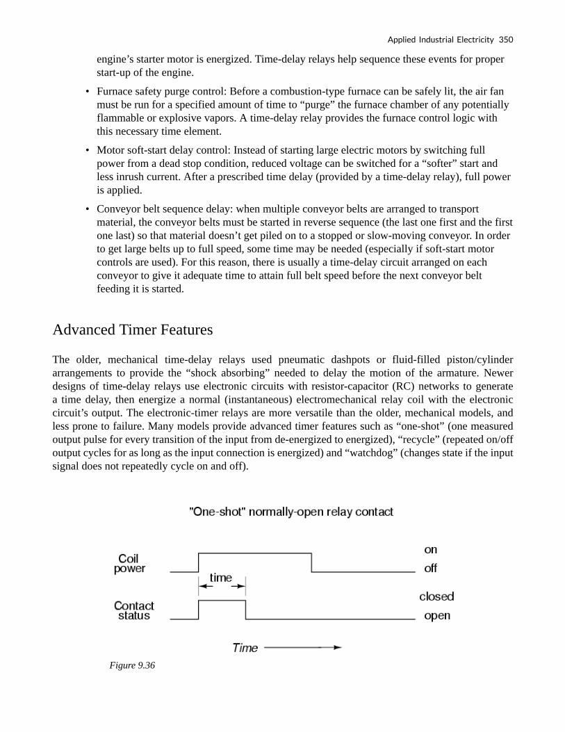
engine’s starter motor is energized. Time-delay relays help sequence these events for proper start-up of the engine.
• Furnace safety purge control: Before a combustion-type furnace can be safely lit, the air fan must be run for a specified amount of time to “purge” the furnace chamber of any potentially flammable or explosive vapors. A time-delay relay provides the furnace control logic with this necessary time element.
• Motor soft-start delay control: Instead of starting large electric motors by switching full power from a dead stop condition, reduced voltage can be switched for a “softer” start and less inrush current. After a prescribed time delay (provided by a time-delay relay), full power is applied.
• Conveyor belt sequence delay: when multiple conveyor belts are arranged to transport material, the conveyor belts must be started in reverse sequence (the last one first and the first one last) so that material doesn’t get piled on to a stopped or slow-moving conveyor. In order to get large belts up to full speed, some time may be needed (especially if soft-start motor controls are used). For this reason, there is usually a time-delay circuit arranged on each conveyor to give it adequate time to attain full belt speed before the next conveyor belt feeding it is started.
Advanced Timer Features
The older, mechanical time-delay relays used pneumatic dashpots or fluid-filled piston/cylinder arrangements to provide the “shock absorbing” needed to delay the motion of the armature. Newer designs of time-delay relays use electronic circuits with resistor-capacitor (RC) networks to generate a time delay, then energize a normal (instantaneous) electromechanical relay coil with the electronic circuit’s output. The electronic-timer relays are more versatile than the older, mechanical models, and less prone to failure. Many models provide advanced timer features such as “one-shot” (one measured output pulse for every transition of the input from de-energized to energized), “recycle” (repeated on/off output cycles for as long as the input connection is energized) and “watchdog” (changes state if the input signal does not repeatedly cycle on and off).
Figure 9.36
Applied Industrial Electricity 350

Figure 9.37
Figure 9.38
“Watchdog” Timer Relays
The “watchdog” timer is especially useful for monitoring of computer systems. If a computer is being used to control a critical process, it is usually recommended to have an automatic alarm to detect computer “lockup” (an abnormal halting of program execution due to any number of causes). An easy way to set up such a monitoring system is to have the computer regularly energize and de-energize the coil of a watchdog timer relay (similar to the output of the “recycle” timer). If the computer execution halts for any reason, the signal it outputs to the watchdog relay coil will stop cycling and freeze in one or the other state. A short time thereafter, the watchdog relay will “time out” and signal a problem.
351 Tony R. Kuphaldt and John R. Haughery

Review
• Time delay relays are built in these four basic modes of contact operation:
• 1: Normally-open, timed-closed. Abbreviated “NOTC”, these relays open
immediately upon coil de-energization and close only if the coil is continuously
energized for the time duration period. Also called normally-open, on-delay relays.
• 2: Normally-open, timed-open. Abbreviated “NOTO”, these relays close
immediately upon coil energization and open after the coil has been de-energized
for the time duration period. Also called normally-open, off delay relays.
• 3: Normally-closed, timed-open. Abbreviated “NCTO”, these relays close
immediately upon coil de-energization and open only if the coil is continuously
energized for the time duration period. Also called normally-closed, on-
delay relays.
• 4: Normally-closed, timed-closed. Abbreviated “NCTC”, these relays open
immediately upon coil energization and close after the coil has been de-energized
for the time duration period. Also called normally-closed, off delay relays.
• One-shot timers provide a single contact pulse of specified duration for each coil
energization (transition from coil off to coil on).
• Recycle timers provide a repeating sequence of on-off contact pulses as long as the
coil is maintained in an energized state.
• Watchdog timers actuate their contacts only if the coil fails to be continuously
sequenced on and off (energized and de-energized) at a minimum frequency.
9.6 “Ladder” Diagrams
Applied Industrial Electricity 352

Figure 9.39
Figure 9.40
Figure 9.41
Ladder diagrams are specialized schematics commonly used to document industrial control logic systems. They are called “ladder” diagrams because they resemble a ladder, with two vertical rails (supply power) and as many “rungs” (horizontal lines) as there are control circuits to represent. If we wanted to draw a simple ladder diagram showing a lamp that is controlled by a hand switch, it would look like this: The “L1” and “L2” designations refer to the two poles of a 120 VAC supply unless otherwise noted. L1 is the “hot” conductor, and L2 is the grounded (“neutral”) conductor. These designations have nothing to do with inductors, just to make things confusing. The actual transformer or generator supplying power to this circuit is omitted for simplicity. In reality, the circuit looks something like this:Typically in industrial relay logic circuits, but not always, the operating voltage for the switch contacts and relay coils will be 120 volts AC. Lower voltage AC and even DC systems are sometimes
353 Tony R. Kuphaldt and John R. Haughery
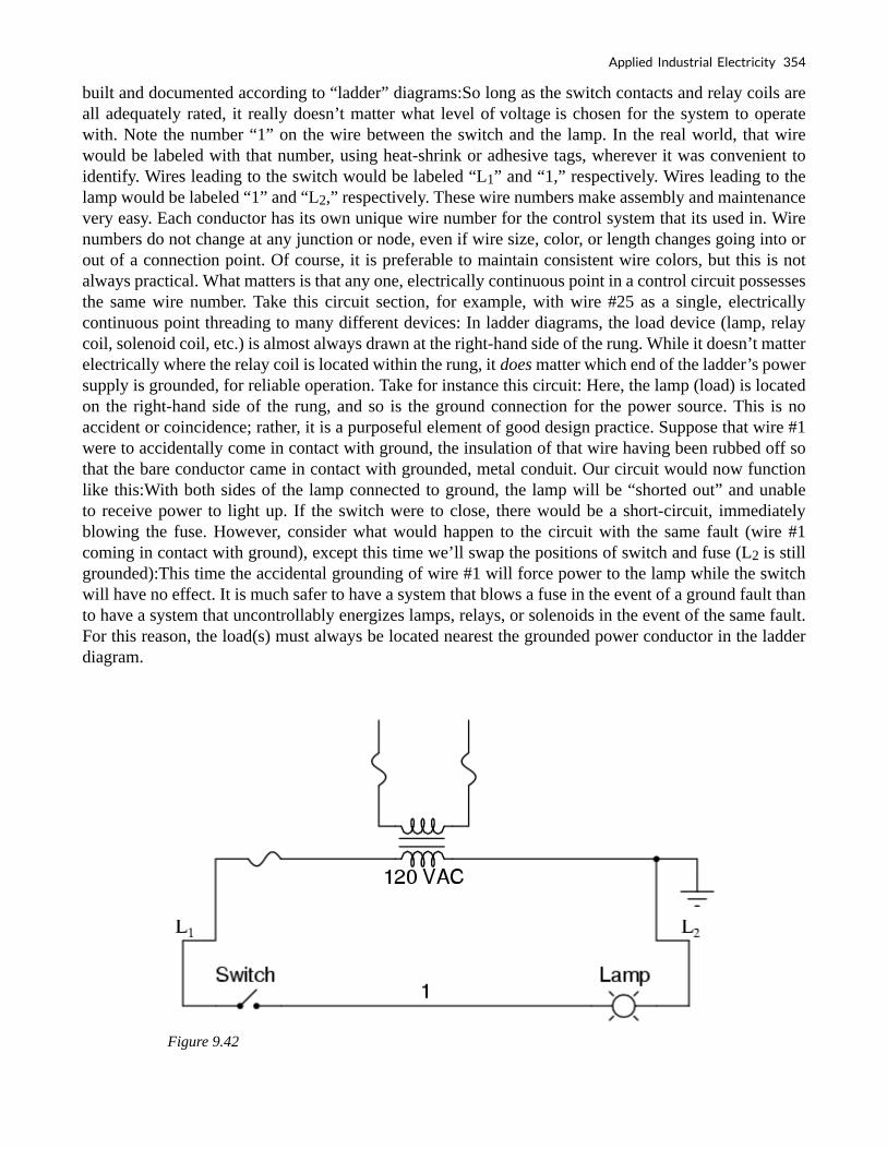
built and documented according to “ladder” diagrams:So long as the switch contacts and relay coils are all adequately rated, it really doesn’t matter what level of voltage is chosen for the system to operate with. Note the number “1” on the wire between the switch and the lamp. In the real world, that wire would be labeled with that number, using heat-shrink or adhesive tags, wherever it was convenient to identify. Wires leading to the switch would be labeled “L1” and “1,” respectively. Wires leading to the lamp would be labeled “1” and “L2,” respectively. These wire numbers make assembly and maintenance very easy. Each conductor has its own unique wire number for the control system that its used in. Wire numbers do not change at any junction or node, even if wire size, color, or length changes going into or out of a connection point. Of course, it is preferable to maintain consistent wire colors, but this is not always practical. What matters is that any one, electrically continuous point in a control circuit possesses the same wire number. Take this circuit section, for example, with wire #25 as a single, electrically continuous point threading to many different devices: In ladder diagrams, the load device (lamp, relay coil, solenoid coil, etc.) is almost always drawn at the right-hand side of the rung. While it doesn’t matter electrically where the relay coil is located within the rung, it does matter which end of the ladder’s power supply is grounded, for reliable operation. Take for instance this circuit: Here, the lamp (load) is located on the right-hand side of the rung, and so is the ground connection for the power source. This is no accident or coincidence; rather, it is a purposeful element of good design practice. Suppose that wire #1 were to accidentally come in contact with ground, the insulation of that wire having been rubbed off so that the bare conductor came in contact with grounded, metal conduit. Our circuit would now function like this:With both sides of the lamp connected to ground, the lamp will be “shorted out” and unable to receive power to light up. If the switch were to close, there would be a short-circuit, immediately blowing the fuse. However, consider what would happen to the circuit with the same fault (wire #1 coming in contact with ground), except this time we’ll swap the positions of switch and fuse (L2 is still grounded):This time the accidental grounding of wire #1 will force power to the lamp while the switch will have no effect. It is much safer to have a system that blows a fuse in the event of a ground fault than to have a system that uncontrollably energizes lamps, relays, or solenoids in the event of the same fault. For this reason, the load(s) must always be located nearest the grounded power conductor in the ladder diagram.
Figure 9.42
Applied Industrial Electricity 354

Figure 9.43
Figure 9.44
355 Tony R. Kuphaldt and John R. Haughery

Review
• Ladder diagrams (sometimes called “ladder logic”) are a type of electrical notation
and symbology frequently used to illustrate how electromechanical switches and
relays are interconnected.
• The two vertical lines are called “rails” and attach to opposite poles of a power
supply, usually 120 volts AC. L1 designates the “hot” AC wire and L2 the “neutral”
(grounded) conductor.
• Horizontal lines in a ladder diagram are called “rungs,” each one representing a
unique parallel circuit branch between the poles of the power supply.
• Typically, wires in control systems are marked with numbers and/or letters for
identification. The rule is, all permanently connected (electrically common) points
must bear the same label.
Applied Industrial Electricity 356

9.7 Digital Logic Functions
Figure 9.45
Figure 9.46
357 Tony R. Kuphaldt and John R. Haughery

Figure 9.47
Figure 9.48
Applied Industrial Electricity 358

Figure 9.49
We can construct simple logic functions for our hypothetical lamp circuit, using multiple contacts, and document these circuits quite easily and understandably with additional rungs to our original “ladder.” If we use standard binary notation for the status of the switches and lamp (0 for unactuated or de-energized; 1 for actuated or energized), a truth table can be made to show how the logic works:Now, the lamp will come on if either contact A or contact B is actuated, because all it takes for the lamp to be energized is to have at least one path for current from wire L1 to wire 1. What we have is a simple OR logic function, implemented with nothing more than contacts and a lamp. We can mimic the AND logic function by wiring the two contacts in series instead of parallel:Now, the lamp energizes only if contact A and contact B are simultaneously actuated. A path exists for current from wire L1 to the lamp (wire 2) if and only if both switch contacts are closed. The logical inversion, or NOT, function can be performed on a contact input simply by using a normally-closed contact instead of a normally-open contact:Now, the lamp energizes if the contact is not actuated, and de-energizes when the contact is actuated.If we take our OR function and invert each “input” through the use of normally-closed contacts, we will end up with a NAND function. In a special branch of mathematics known as Boolean algebra, this effect of gate function identity changing with the inversion of input signals is described by DeMorgan’s Theorem, a subject to be explored in more detail in a later chapter.The lamp will be energized if either contact is unactuated. It will go out only if both contacts are actuated simultaneously. Likewise, if we take our AND function and invert each “input” through the use of normally-closed contacts, we will end up with a NOR function:A pattern quickly reveals itself when ladder circuits are compared with their logic gate counterparts:
• Parallel contacts are equivalent to an OR gate.
• Series contacts are equivalent to an AND gate.
359 Tony R. Kuphaldt and John R. Haughery
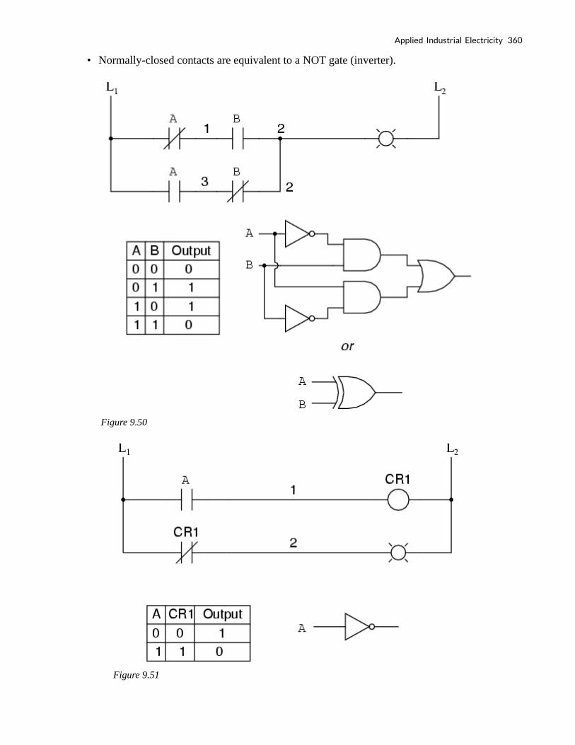
• Normally-closed contacts are equivalent to a NOT gate (inverter).
Figure 9.50
Figure 9.51
Applied Industrial Electricity 360

Figure 9.52
We can build combinational logic functions by grouping contacts in series-parallel arrangements, as well. In the following example, we have an Exclusive-OR function built from a combination of AND, OR, and inverter (NOT) gates:The top rung (NC contact A in series with NO contact B) is the equivalent of the top NOT/AND gate combination. The bottom rung (NO contact A in series with NC contact B) is the equivalent of the bottom NOT/AND gate combination. The parallel connection between the two rungs at wire number 2 forms the equivalent of the OR gate, in allowing either rung 1 or rung 2 to energize the lamp. To make the Exclusive-OR function, we had to use two contacts per input: one for direct input and the other for “inverted” input. The two “A” contacts are physically actuated by the same mechanism, as are the two “B” contacts. The common association between contacts is denoted by the label of the contact. There is no limit to how many contacts per switch can be represented in a ladder diagram, as each new contact on any switch or relay (either normally-open or normally-closed) used in the diagram is simply marked with the same label. Sometimes, multiple contacts on a single switch (or relay) are designated by a compound labels, such as “A-1” and “A-2” instead of two “A” labels. This may be especially useful if you want to specifically designate which set of contacts on each switch or relay is being used for which part of a circuit. For simplicity’s sake, I’ll refrain from such elaborate
361 Tony R. Kuphaldt and John R. Haughery

labeling in this lesson. If you see a common label for multiple contacts, you know those contacts are all actuated by the same mechanism. If we wish to invert the output of any switch-generated logic function, we must use a relay with a normally-closed contact. For instance, if we want to energize a load based on the inverse, or NOT, of a normally-open contact, we could do this:We will call the relay, “control relay 1,” or CR1. When the coil of CR1 (symbolized with the pair of parentheses on the first rung) is energized, the contact on the second rung opens, thus de-energizing the lamp. From switch A to the coil of CR1, the logic function is noninverted. The normally-closed contact actuated by relay coil CR1 provides a logical inverter function to drive the lamp opposite that of the switch’s actuation status. Applying this inversion strategy to one of our inverted-input functions created earlier, such as the OR-to-NAND, we can invert the output with a relay to create a noninverted function:From the switches to the coil of CR1, the logical function is that of a NAND gate. CR1‘s normally-closed contact provides one final inversion to turn the NAND function into an AND function.
Review
• Parallel contacts are logically equivalent to an OR gate.
• Series contacts are logically equivalent to an AND gate.
• Normally closed (N.C.) contacts are logically equivalent to a NOT gate.
• A relay must be used to invert the output of a logic gate function, while simple
normally-closed switch contacts are sufficient to represent inverted gate inputs.
Applied Industrial Electricity 362
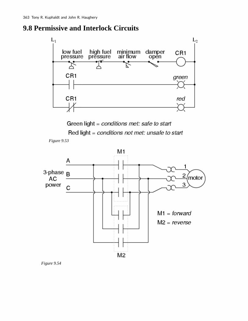
9.8 Permissive and Interlock Circuits
Figure 9.53
Figure 9.54
363 Tony R. Kuphaldt and John R. Haughery

Figure 9.55
Figure 9.56
A practical application of switch and relay logic is in control systems where several process conditions have to be met before a piece of equipment is allowed to start. A good example of this is burner control for large combustion furnaces. In order for the burners in a large furnace to be started safely, the control system requests “permission” from several process switches, including high and low fuel pressure, air fan flow check, exhaust stack damper position, access door position, etc. Each process condition is called a permissive, and each permissive switch contact is wired in series, so that if any one of them detects an unsafe condition, the circuit will be opened:If all permissive conditions are met, CR1 will energize and the green lamp will be lit. In real life, more than just a green lamp would be energized: usually, a control relay or fuel valve solenoid would be placed in that rung of the circuit to be energized when all the permissive contacts were “good:” that is, all closed. If any one of the permissive conditions are not met, the series string of switch contacts will be broken, CR2 will de-energize, and the red lamp will light. Note that the high fuel pressure contact is normally-closed. This is because we want the switch contact to open if the fuel pressure gets too high. Since the “normal” condition of any pressure switch is when zero (low) pressure is being applied to it, and we want this switch to open with excessive (high) pressure, we must choose a switch that is closed in its normal state. Another practical application of relay logic is in control systems where we want to ensure two incompatible events cannot occur at the same time. An example of this is in reversible motor control, where two motor contactors are wired to switch polarity (or phase sequence) to an electric motor, and we don’t want the forward and reverse contactors energized simultaneously:When contactor M1 is energized, the 3 phases (A, B, and C) are connected directly to terminals 1, 2, and 3 of the motor, respectively. However, when contactor M2 is energized, phases A and B are reversed, A going to motor terminal 2 and B going to motor terminal
Applied Industrial Electricity 364

1. This reversal of phase wires results in the motor spinning the opposite direction. Let’s examine the control circuit for these two contactors:Take note of the normally-closed “OL” contact, which is the thermal overload contact activated by the “heater” elements wired in series with each phase of the AC motor. If the heaters get too hot, the contact will change from its normal (closed) state to being open, which will prevent either contactor from energizing. This control system will work fine, so long as no one pushes both buttons at the same time. If someone were to do that, phases A and B would be short-circuited together by virtue of the fact that contactor M1 sends phases A and B straight to the motor and contactor M2 reverses them; phase A would be shorted to phase B and vice versa. Obviously, this is a bad control system design! To prevent this occurrence from happening, we can design the circuit so that the energization of one contactor prevents the energization of the other. This is called interlocking, and it is accomplished through the use of auxiliary contacts on each contactor, as such:Now, when M1 is energized, the normally-closed auxiliary contact on the second rung will be open, thus preventing M2 from being energized, even if the “Reverse” pushbutton is actuated. Likewise, M1‘s energization is prevented when M2 is energized. Note, as well, how additional wire numbers (4 and 5) were added to reflect the wiring changes. It should be noted that this is not the only way to interlock contactors to prevent a short-circuit condition. Some contactors come equipped with the option of a mechanical interlock: a lever joining the armatures of two contactors together so that they are physically prevented from simultaneous closure. For additional safety, electrical interlocks may still be used, and due to the simplicity of the circuit there is no good reason not to employ them in addition to mechanical interlocks.
Review
• Switch contacts installed in a rung of ladder logic designed to interrupt a circuit if
certain physical conditions are not met are called permissive contacts, because the
system requires permission from these inputs to activate.
• Switch contacts designed to prevent a control system from taking two incompatible
actions at once (such as powering an electric motor forward and backward
simultaneously) are called interlocks.
365 Tony R. Kuphaldt and John R. Haughery

10. MOTOR CIRCUITS AND CONTROL
10.1 Motor Control Circuits
The interlock contacts installed in the previous section’s motor control circuit work fine, but the motor will run only as long as each push button switch is held down. If we wanted to keep the motor running even after the operator takes his or her hand off the control switch(es), we could change the circuit in a couple of different ways: we could replace the push button switches with toggle switches, or we could add some more relay logic to “latch” the control circuit with a single, momentary actuation of either switch. Let’s see how the second approach is implemented since it is commonly used in industry:
Figure 10.1
When the “Forward” pushbutton is actuated, M1 will energize, closing the normally-open auxiliary contact in parallel with that switch. When the pushbutton is released, the closed M1 auxiliary contact will maintain current to the coil of M1, thus latching the “Forward” circuit in the “on” state. The same sort of thing will happen when the “Reverse” pushbutton is pressed. These parallel auxiliary contacts are sometimes referred to as seal-in contacts, the word “seal” meaning essentially the same thing as the word latch. However, this creates a new problem: how to stop the motor! As the circuit exists right now, the motor will run either forward or backward once the corresponding pushbutton switch is pressed and will continue to run as long as there is power. To stop either circuit (forward or backward), we require some means for the operator to interrupt power to the motor contactors. We’ll call this new switch, Stop:
366

Figure 10.2
Now, if either forward or reverse circuits are latched, they may be “unlatched” by momentarily pressing the “Stop” pushbutton, which will open either forward or reverse circuit, de-energizing the energized contactor, and returning the seal-in contact to its normal (open) state. The “Stop” switch, having normally-closed contacts, will conduct power to either forward or reverse circuits when released. So far, so good. Let’s consider another practical aspect of our motor control scheme before we quit adding to it. If our hypothetical motor turned a mechanical load with a lot of momentum, such as a large air fan, the motor might continue to coast for a substantial amount of time after the stop button had been pressed. This could be problematic if an operator were to try to reverse the motor direction without waiting for the fan to stop turning. If the fan was still coasting forward and the “Reverse” pushbutton was pressed, the motor would struggle to overcome that inertia of the large fan as it tried to begin turning in reverse, drawing excessive current and potentially reducing the life of the motor, drive mechanisms, and fan. What we might like to have is some kind of a time-delay function in this motor control system to prevent such a premature startup from happening. Let’s begin by adding a couple of time-delay relay coils, one in parallel with each motor contactor coil. If we use contacts that delay returning to their normal state, these relays will provide us a “memory” of which direction the motor was last powered to turn. What we want each time-delay contact to do is to open the starting-switch leg of the opposite rotation circuit for several seconds, while the fan coasts to a halt.
367 Tony R. Kuphaldt and John R. Haughery

Figure 10.3
If the motor has been running in the forward direction, both M1 and TD1 will have been energized. This being the case, the normally-closed, timed-closed contact of TD1 between wires 8 and 5 will have immediately opened the moment TD1 was energized. When the stop button is pressed, contact TD1 waits for the specified amount of time before returning to its normally-closed state, thus holding the reverse pushbutton circuit open for the duration so M2 can’t be energized. When TD1 times out, the contact will close and the circuit will allow M2 to be energized if the reverse pushbutton is pressed. In like manner, TD2 will prevent the “Forward” pushbutton from energizing M1 until the prescribed time delay after M2 (and TD2) have been de-energized. The careful observer will notice that the time-interlocking functions of TD1 and TD2 render the M1 and M2 interlocking contacts redundant. We can get rid of auxiliary contacts M1 and M2 for interlocks and just use TD1 and TD2‘s contacts, since they immediately open when their respective relay coils are energized, thus “locking out” one contactor if the other is energized. Each time delay relay will serve a dual purpose: preventing the other contactor from energizing while the motor is running and preventing the same contactor from energizing until a prescribed time after motor shutdown. The resulting circuit has the advantage of being simpler than the previous example:
Applied Industrial Electricity 368
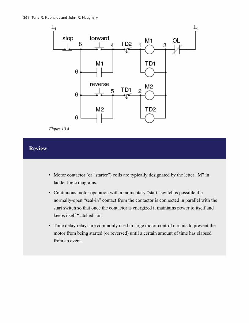
Figure 10.4
Review
• Motor contactor (or “starter”) coils are typically designated by the letter “M” in
ladder logic diagrams.
• Continuous motor operation with a momentary “start” switch is possible if a
normally-open “seal-in” contact from the contactor is connected in parallel with the
start switch so that once the contactor is energized it maintains power to itself and
keeps itself “latched” on.
• Time delay relays are commonly used in large motor control circuits to prevent the
motor from being started (or reversed) until a certain amount of time has elapsed
from an event.
369 Tony R. Kuphaldt and John R. Haughery

10.2 Contactors
All About Contactors
Figure 10.5
When a relay is used to switch a large amount of electrical power through its contacts, it is designated by a special name: contactor. Contactors typically have multiple contacts, and those contacts are usually (but not always) normally-open, so that power to the load is shut off when the coil is de-energized. Perhaps the most common industrial use for contactors is the control of electric motors.The top three contacts switch the respective phases of the incoming 3-phase AC power, typically at least 480 Volts for motors 1 horsepower or greater. The lowest contact is an “auxiliary” contact which has a current rating much lower than that of the large motor power contacts, but is actuated by the same armature as the power contacts. The auxiliary contact is often used in a relay logic circuit, or for some other part of the motor control scheme, typically switching 120 Volt AC power instead of the motor voltage. One contactor may have several auxiliary contacts, either normally-open or normally-closed if required.
The three “opposed-question-mark” shaped devices in series with each phase going to the motor are called overload heaters. Each “heater” element is a low-resistance strip of metal intended to heat up as the motor draws current. If the temperature of any of these heater elements reaches a critical point (equivalent to a moderate overloading of the motor), a normally-closed switch contact (not shown in the diagram) will spring open. This normally-closed contact is usually connected in series with the relay coil, so that when it opens the relay will automatically de-energize, thereby shutting off power to the motor. We will see more of this overload protection wiring in the next chapter. Overload heaters are intended to provide overcurrent protection for large electric motors, unlike circuit breakers and fuses which serve the primary purpose of providing overcurrent protection for power conductors. Overload heater function is often misunderstood. They are not fuses; that is, it is not their function to burn open and directly break the circuit as a fuse is designed to do. Rather, overload heaters are designed to thermally mimic the heating characteristic of the particular electric motor to be protected. All motors have thermal characteristics, including the amount of heat energy generated by resistive dissipation (I2R), the thermal transfer characteristics of heat “conducted” to the cooling medium through the metal frame of the motor, the physical mass and specific heat of the materials constituting the motor, etc. These characteristics are mimicked by the overload heater on a miniature scale: when the motor heats up
Applied Industrial Electricity 370

toward its critical temperature, so will the heater toward its critical temperature, ideally at the same rate and approach curve. Thus, the overload contact, in sensing heater temperature with a thermomechanical mechanism, will sense an analog of the real motor. If the overload contact trips due to excessive heater temperature, it will be an indication that the real motor has reached its critical temperature (or, would have done so in a short while). After tripping, the heaters are supposed to cool down at the same rate and approach curve as the real motor, so that they indicate an accurate proportion of the motor’s thermal condition, and will not allow power to be re-applied until the motor is truly ready for start-up again.
Three-Phase Electric Motor Contactor
Shown here is a contactor for a three-phase electric motor, installed on a panel as part of an electrical control system at a municipal water treatment plant:
371 Tony R. Kuphaldt and John R. Haughery

Figure 10.6
Applied Industrial Electricity 372

Figure 10.7
Three-phase, 480 volt AC power comes into the three normally-open contacts at the top of the contactor via screw terminals labeled “L1,” “L2,” and “L3” (The “L2” terminal is hidden behind a square-shaped “snubber” circuit connected across the contactor’s coil terminals). Power to the motor exits the overload heater assembly at the bottom of this device via screw terminals labeled “T1,” “T2,” and “T3.” The overload heater units themselves are black, square-shaped blocks with the label “W34,” indicating a particular thermal response for a certain horsepower and temperature rating of the electric motor. If an electric motor of differing power and/or temperature ratings were to be substituted for the one presently in service, the overload heater units would have to be replaced with units having a thermal response suitable for the new motor. The motor manufacturer can provide information on the appropriate heater units to use. A white push button located between the “T1” and “T2” line heaters serves as a way to manually reset the normally-closed switch contact back to its normal state after having been tripped by excessive heater temperature. Wire connections to the “overload” switch contact may be seen at the lower-right of the photograph, near a label reading “NC” (normally-closed). On this particular overload unit, a small “window” with the label “Tripped” indicates a tripped condition by means of a colored flag. In this photograph, there is no “tripped” condition, and the indicator appears clear. As a footnote, heater elements may be used as a crude current shunt resistor for determining whether or not a motor is drawing current when the contactor is closed. There may be times when you’re working on a motor control circuit, where the contactor is located far away from the motor itself. How do you know if the motor is consuming power when the contactor coil is energized and the armature has been pulled in? If the motor’s windings are burnt open, you could be sending voltage to the motor through the contactor contacts, but still, have zero current, and thus no motion from the motor shaft. If a clamp-on ammeter isn’t available to measure line current, you can take your multimeter and measure millivoltage across each heater element: if the current is zero, the voltage across the heater will be zero (unless the heater element itself is open, in which case the voltage across it will be large); if there is current going to the motor through that phase of the contactor, you will read a definite millivoltage across that heater. This is an especially useful trick to use for troubleshooting 3-phase AC motors, to see if one phase winding
373 Tony R. Kuphaldt and John R. Haughery

is burnt open or disconnected, which will result in a rapidly destructive condition known as “single-phasing.” If one of the lines carrying power to the motor is open, it will not have any current through it (as indicated by a 0.00 mV reading across its heater), although the other two lines will (as indicated by small amounts of voltage dropped across the respective heaters).
Review
• A contactor is a large relay, usually used to switch current to an electric motor or
another high-power load.
• Large electric motors can be protected from overcurrent damage through the use
of overload heaters and overload contacts. If the series-connected heaters get too
hot from excessive current, the normally-closed overload contact will open, de-
energizing the contactor sending power to the motor.
Applied Industrial Electricity 374

11. CONDUCTORS
11.1 Introduction to Conductance and Conductors
By now you should be well aware of the correlation between electrical conductivity and certain types of materials. Those materials allowing for easy passage of free electrons are called conductors, while those materials impeding the passage of free electrons are called insulators.
Unfortunately, the scientific theories explaining why certain materials conduct and others don’t are quite complex, rooted in quantum mechanical explanations in how electrons are arranged around the nuclei of atoms. Contrary to the well-known “planetary” model of electrons whirling around an atom’s nucleus as well-defined chunks of matter in circular or elliptical orbits, electrons in “orbit” don’t really act like pieces of matter at all. Rather, they exhibit the characteristics of both particle and wave, their behavior constrained by placement within distinct zones around the nucleus referred to as “shells” and “subshells.” Electrons can occupy these zones only in a limited range of energies depending on the particular zone and how occupied that zone is with other electrons. If electrons really did act like tiny planets held in orbit around the nucleus by electrostatic attraction, their actions described by the same laws describing the motions of real planets, there could be no real distinction between conductors and insulators, and chemical bonds between atoms would not exist in the way they do now. It is the discrete, “quantitized” nature of electron energy and placement described by quantum physics that gives these phenomena their regularity.
Excited-state Atom
When an electron is free to assume higher energy states around an atom’s nucleus (due to its placement in a particular “shell”), it may be free to break away from the atom and comprise part of an electric current through the substance.
Ground-state Atom
If the quantum limitations imposed on an electron deny it this freedom, however, the electron is considered to be “bound” and cannot break away (at least not easily) to constitute a current. The former scenario is typical of conducting materials, while the latter is typical of insulating materials.
Some textbooks will tell you that an element’s electrical conductivity is exclusively determined by the number of electrons residing in the atoms’ outer “shell” (called the valence shell), but this is an oversimplification, as any examination of conductivity versus valence electrons in a table of elements will confirm. The true complexity of the situation is further revealed when the conductivity of molecules (collections of atoms bound to one another by electron activity) is considered.
A good example of this is the element carbon, which comprises materials of vastly differing conductivity: graphite and diamond. Graphite is a fair conductor of electricity, while diamond is
375

practically an insulator (stranger yet, it is technically classified as a semiconductor, which in its pure form acts as an insulator, but can conduct under high temperatures and/or the influence of impurities). Both graphite and diamond are composed of the exact same types of atoms: carbon, with 6 protons, 6 neutrons and 6 electrons each. The fundamental difference between graphite and diamond being that graphite molecules are flat groupings of carbon atoms while diamond molecules are tetrahedral (pyramid-shaped) groupings of carbon atoms.
The intentional introduction of impurities into an intrinsic semiconductor for the purpose of altering its electrical, optical, and structural properties is called doping. If atoms of carbon are joined to other types of atoms to form compounds, electrical conductivity becomes altered once again. Silicon carbide, a compound of the elements silicon and carbon, exhibits nonlinear behavior: its electrical resistance decreases with increases in applied voltage! Hydrocarbon compounds (such as the molecules found in oils) tend to be very good insulators. As you can see, a simple count of valence electrons in an atom is a poor indicator of a substance’s electrical conductivity.
All metallic elements are good conductors of electricity, due to the way the atoms bond with each other. The electrons of the atoms comprising a mass of metal are so uninhibited in their allowable energy states that they float freely between the different nuclei in the substance, readily motivated by any electric field. The electrons are so mobile, in fact, that they are sometimes described by scientists as an electron gas, or even an electron sea in which the atomic nuclei rest. This electron mobility accounts for some of the other common properties of metals: good heat conductivity, malleability and ductility (easily formed into different shapes), and a lustrous finish when pure.
Thankfully, the physics behind all this is mostly irrelevant to our purposes here. Suffice it to say that some materials are good conductors, some are poor conductors, and some are in between. For now it is good enough to simply understand that these distinctions are determined by the configuration of the electrons around the constituent atoms of the material.
An important step in getting electricity to do our bidding is to be able to construct paths for current to flow with controlled amounts of resistance. It is also vitally important that we be able to prevent current from flowing where we don’t want it to, by using insulating materials. However, not all conductors are the same, and neither are all insulators. We need to understand some of the characteristics of common conductors and insulators, and be able to apply these characteristics to specific applications.
Almost all conductors possess a certain, measurable resistance (special types of materials called superconductors possess absolutely no electrical resistance, but these are not ordinary materials, and they must be held in special conditions in order to be super conductive). Typically, we assume the resistance of the conductors in a circuit to be zero, and we expect that current passes through them without producing any appreciable voltage drop. In reality, however, there will almost always be a voltage drop along the (normal) conductive pathways of an electric circuit, whether we want a voltage drop to be there or not:
Applied Industrial Electricity 376

Figure 11.1
In order to calculate what these voltage drops will be in any particular circuit, we must be able to ascertain the resistance of ordinary wire, knowing the wire size and diameter. Some of the following sections of this chapter will address the details of doing this.
Review
• Electrical conductivity of a material is determined by the configuration of electrons
in that materials atoms and molecules (groups of bonded atoms).
• All normal conductors possess resistance to some degree.
• Current flowing through a conductor with (any) resistance will produce some
amount of voltage drop across the length of that conductor.
11.2 Conductor Size
It should be common-sense knowledge that liquids flow through large-diameter pipes easier than they do through small-diameter pipes (if you would like a practical illustration, try drinking a liquid through straws of different diameters). The same general principle holds for the flow of electrons through conductors: the broader the cross-sectional area (thickness) of the conductor, the more room for electrons to flow, and consequently, the easier it is for flow to occur (less resistance).
377 Tony R. Kuphaldt and John R. Haughery

Two Basic Varieties of Electrical Wire: Solid and Stranded
Electrical wire is usually round in cross-section (although there are some unique exceptions to this rule), and comes in two basic varieties: solid and stranded. Solid copper wire is just as it sounds: a single, solid strand of copper the whole length of the wire. Stranded wire is composed of smaller strands of solid copper wire twisted together to form a single, larger conductor. The greatest benefit of stranded wire is its mechanical flexibility, being able to withstand repeated bending and twisting much better than solid copper (which tends to fatigue and break after time).
Wire size can be measured in several ways. We could speak of a wire’s diameter, but since its really the cross-sectional area that matters most regarding the flow of electrons, we are better off designating wire size in terms of area.
Example 11.1
The wire cross-section picture shown above is, of course, not drawn to scale. The diameter is
shown as being 0.1019 inches. Calculating the area of the cross-section with the formula Area
= πr2, we get an area of 0.008155 square inches:
A=(3.1416) (\frac{0.1019 \text{ inches}}{2})^2
Applied Industrial Electricity 378

These are fairly small numbers to work with, so wire sizes are often expressed in measures of thousandths-of-an-inch, or mils. For the illustrated example, we would say that the diameter of the wire was 101.9 mils (0.1019 inch times 1000). We could also, if we wanted, express the area of the wire in the unit of square mils, calculating that value with the same circle-area formula, Area = πr2:
Example 11.2
379 Tony R. Kuphaldt and John R. Haughery

Calculating the Circular-mil Area of a Wire
However, electricians and others frequently concerned with wire size use another unit of area measurement tailored specifically for wire’s circular cross-section. This special unit is called the circular mil (sometimes abbreviated cmil). The sole purpose for having this special unit of measurement is to eliminate the need to invoke the factor π (3.1415927 . . .) in the formula for calculating area, plus the need to figure wire radius when you’ve been given diameter. The formula for calculating the circular-mil area of a circular wire is very simple:
Circular Wire Area Formula
Because this is a unit of area measurement, the mathematical power of 2 is still in effect (doubling the width of a circle will always quadruple its area, no matter what units are used, or if the width of that circle is expressed in terms of radius or diameter). To illustrate the difference between measurements in square mils and measurements in circular mils, I will compare a circle with a square, showing the area of each shape in both unit measures:
Applied Industrial Electricity 380

Figure 11.4
And for another size of wire:
381 Tony R. Kuphaldt and John R. Haughery

Figure 11.5
Obviously, the circle of a given diameter has less cross-sectional area than a square of width and height equal to the circle’s diameter: both units of area measurement reflect that. However, it should be clear that the unit of “square mil” is really tailored for the convenient determination of a square’s area, while “circular mil” is tailored for the convenient determination of a circle’s area: the respective formula for each is simpler to work with. It must be understood that both units are valid for measuring the area of a shape, no matter what shape that may be. The conversion between circular mils and square mils is a simple ratio: there are π (3.1415927 . . .) square mils to every 4 circular mils.
Measuring Cross-Sectional Wire Area with Gauge
Another measure of cross-sectional wire area is the gauge. The gauge scale is based on whole numbers rather than fractional or decimal inches. The larger the gauge number, the skinnier the wire; the smaller the gauge number, the fatter the wire. For those acquainted with shotguns, this inversely-proportional measurement scale should sound familiar.
The table at the end of this section equates gauge with inch diameter, circular mils, and square inches for solid wire. The larger sizes of wire reach an end of the common gauge scale (which naturally tops out at a value of 1), and are represented by a series of zeros. “3/0” is another way to represent “000,” and is pronounced “triple-ought.” Again, those acquainted with shotguns should recognize the terminology, strange as it may sound. To make matters even more confusing, there is more than one gauge “standard” in use around the world. For electrical conductor sizing, the American Wire Gauge (AWG), also known as the Brown and Sharpe (B&S) gauge, is the measurement system of
Applied Industrial Electricity 382

choice. In Canada and Great Britain, the British Standard Wire Gauge (SWG) is the legal measurement system for electrical conductors. Other wire gauge systems exist in the world for classifying wire diameter, such as the Stubs steel wire gauge and the Steel Music Wire Gauge (MWG), but these measurement systems apply to non-electrical wire use.
The American Wire Gauge (AWG) measurement system, despite its oddities, was designed with a purpose: for every three steps in the gauge scale, wire area (and weight per unit length) approximately doubles. This is a handy rule to remember when making rough wire size estimations!
For very large wire sizes (fatter than 4/0), the wire gauge system is typically abandoned for cross-sectional area measurement in thousands of circular mils (MCM), borrowing the old Roman numeral “M” to denote a multiple of “thousand” in front of “CM” for “circular mils.” The following table of wire sizes does not show any sizes bigger than 4/0 gauge, because solid copper wire becomes impractical to handle at those sizes. Stranded wire construction is favored, instead.
Wire Table For Solid, Round Copper Conductors
383 Tony R. Kuphaldt and John R. Haughery

Size Diameter Cross-sectional area Weight
AWG Inches cir. mils sq. inches lb/1000 ft
4/0 0.4600 211,600 0.1662 640.5
3/0 0.4096 167,800 0.1318 507.9
2/0 0.3648 133,100 0.1045 402.8
1/0 0.3249 105,500 0.08289 319.5
1 0.2893 83,690 0.06573 253.5
2 0.2576 66,370 0.05213 200.9
3 0.2294 52,630 0.04134 159.3
4 0.2043 41,740 0.03278 126.4
5 0.1819 33,100 0.02600 100.2
6 0.1620 26,250 0.02062 79.46
7 0.1443 20,820 0.01635 63.02
8 0.1285 16,510 0.01297 49.97
9 0.1144 13,090 0.01028 39.63
10 0.1019 10,380 0.008155 31.43
11 0.09074 8,234 0.006467 24.92
12 0.08081 6,530 0.005129 19.77
13 0.07196 5,178 0.004067 15.68
14 0.06408 4,107 0.003225 12.43
15 0.05707 3,257 0.002558 9.858
16 0.05082 2,583 0.002028 7.818
17 0.04526 2,048 0.001609 6.200
18 0.04030 1,624 0.001276 4.917
19 0.03589 1,288 0.001012 3.899
20 0.03196 1,022 0.0008023 3.092
21 0.02846 810.1 0.0006363 2.452
22 0.02535 642.5 0.0005046 1.945
23 0.02257 509.5 0.0004001 1.542
24 0.02010 404.0 0.0003173 1.233
25 0.01790 320.4 0.0002517 0.9699
Applied Industrial Electricity 384
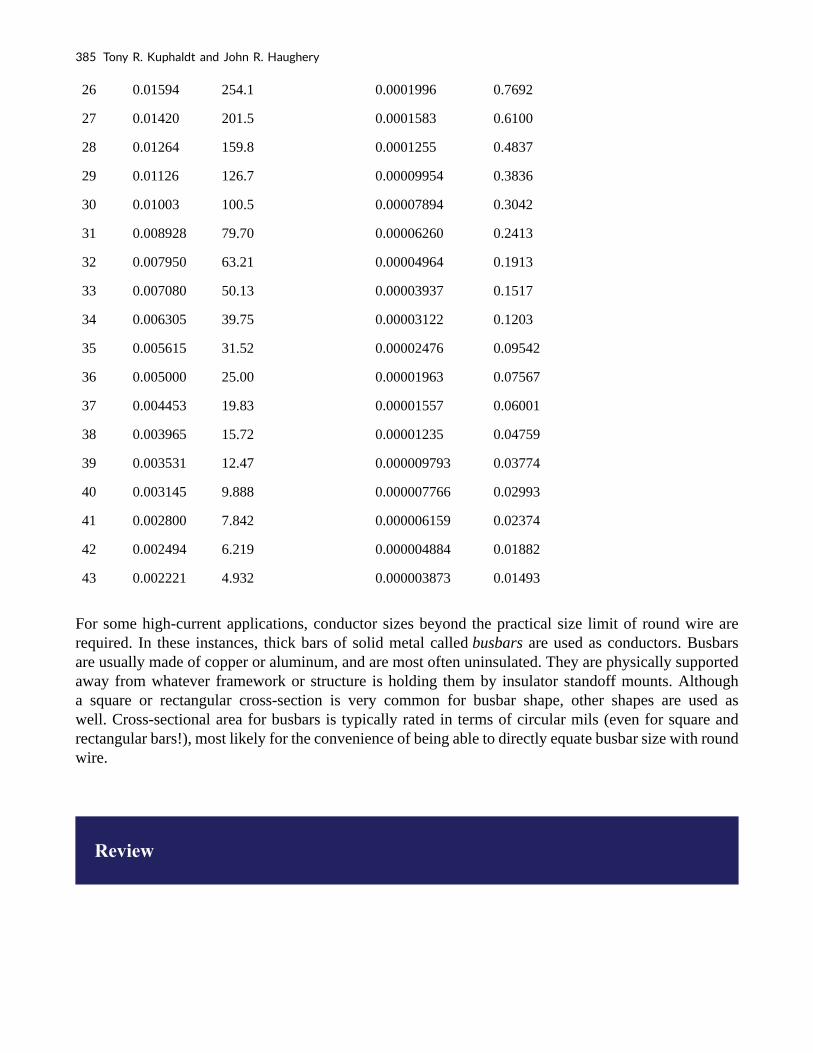
26 0.01594 254.1 0.0001996 0.7692
27 0.01420 201.5 0.0001583 0.6100
28 0.01264 159.8 0.0001255 0.4837
29 0.01126 126.7 0.00009954 0.3836
30 0.01003 100.5 0.00007894 0.3042
31 0.008928 79.70 0.00006260 0.2413
32 0.007950 63.21 0.00004964 0.1913
33 0.007080 50.13 0.00003937 0.1517
34 0.006305 39.75 0.00003122 0.1203
35 0.005615 31.52 0.00002476 0.09542
36 0.005000 25.00 0.00001963 0.07567
37 0.004453 19.83 0.00001557 0.06001
38 0.003965 15.72 0.00001235 0.04759
39 0.003531 12.47 0.000009793 0.03774
40 0.003145 9.888 0.000007766 0.02993
41 0.002800 7.842 0.000006159 0.02374
42 0.002494 6.219 0.000004884 0.01882
43 0.002221 4.932 0.000003873 0.01493
For some high-current applications, conductor sizes beyond the practical size limit of round wire are required. In these instances, thick bars of solid metal called busbars are used as conductors. Busbars are usually made of copper or aluminum, and are most often uninsulated. They are physically supported away from whatever framework or structure is holding them by insulator standoff mounts. Although a square or rectangular cross-section is very common for busbar shape, other shapes are used as well. Cross-sectional area for busbars is typically rated in terms of circular mils (even for square and rectangular bars!), most likely for the convenience of being able to directly equate busbar size with round wire.
Review
385 Tony R. Kuphaldt and John R. Haughery

• Current flows through large-diameter wires easier than small-diameter wires, due to
the greater cross-sectional area they have in which to move.
• Rather than measure small wire sizes in inches, the unit of “mil” (1/1000 of an inch)
is often employed.
• The cross-sectional area of a wire can be expressed in terms of square units (square
inches or square mils), circular mils, or “gauge” scale.
• Calculating square-unit wire area for a circular wire involves the circle area
formula:
• A = πr2 (square units)
• Calculating circular-mil wire area for a circular wire is much simpler, due to the fact
that the unit of “circular mil” was sized just for this purpose: to eliminate the “pi”
and the d/2 (radius) factors in the formula.
• A = d2 (circular units)
• There are π (3.1416) square mils for every 4 circular mils.
• The gauge system of wire sizing is based on whole numbers, larger numbers
representing smaller-area wires and vice versa. Wires thicker than 1 gauge are
represented by zeros: 0, 00, 000, and 0000 (spoken “single-ought,” “double-ought,”
“triple-ought,” and “quadruple-ought.”
• Very large wire sizes are rated in thousands of circular mils (MCM’s), typical for
busbars and wire sizes beyond 4/0.
• Busbars are solid bars of copper or aluminum used in high-current circuit
construction. Connections made to busbars are usually welded or bolted, and the
busbars are often bare (uninsulated), supported away from metal frames through the
use of insulating standoffs.
11.3 Conductor Ampacity
The smaller the cross-sectional area of any given wire, the greater the resistance for any given length, all
Applied Industrial Electricity 386
other factors being equal. A wire with greater resistance will dissipate a greater amount of heat energy for any given amount of current, the power being equal to P=I2R.
Dissipated power due to a conductor’s resistance manifests itself in the form of heat, and excessive heat can be damaging to a wire (not to mention objects near the wire), especially considering the fact that most wires are insulated with a plastic or rubber coating, which can melt and burn. Thin wires will, therefore, tolerate less current than thick wires, all other factors being equal. A conductor’s current-carrying limit is known as its ampacity.
Primarily for reasons of safety, certain standards for electrical wiring have been established within the United States, and are specified in the National Electrical Code (NEC). Typical NEC wire ampacity tables will show allowable maximum currents for different sizes and applications of wire. Though the melting point of copper theoretically imposes a limit on wire ampacity, the materials commonly employed for insulating conductors melt at temperatures far below the melting point of copper, and so practical ampacity ratings are based on the thermal limits of the insulation. Voltage dropped as a result of excessive wire resistance is also a factor in sizing conductors for their use in circuits, but this consideration is better assessed through more complex means (which we will cover in this chapter). A table derived from an NEC listing is shown for example:
Table 11.2 Copper Conductor Ampacities, in Free Air at 30 Degrees C
Insulation: RUW, T THW, THWN FEP, FEPB
Type: TW RUH THHN, XHHW
387 Tony R. Kuphaldt and John R. Haughery

Size Current Rating Current Rating Current Rating
AWG @ 60 degrees C @ 75 degrees C @ 90 degrees C
20 *9 – *12.5
19 *13 – 18
16 *18 – 24
14 25 30 35
12 30 35 40
10 40 50 55
8 60 70 80
6 80 95 105
4 105 125 140
2 140 170 190
1 165 195 220
1/0 195 230 260
2/0 225 265 300
3/0 260 310 350
4/0 300 360 405
* = estimated values; normally, these small wire sizes are not manufactured with these insulation types
Notice the substantial ampacity differences between same-size wires with different types of insulation. This is due, again, to the thermal limits (60°, 75°, 90°) of each type of insulation material.
These ampacity ratings are given for copper conductors in “free air” (maximum typical air circulation), as opposed to wires placed in conduit or wire trays. As you will notice, the table fails to specify ampacities for small wire sizes. This is because the NEC concerns itself primarily with power wiring (large currents, big wires) rather than with wires common to low-current electronic work.
There is meaning in the letter sequences used to identify conductor types, and these letters usually refer to properties of the conductor’s insulating layer(s). Some of these letters symbolize individual properties of the wire while others are simply abbreviations. For example, the letter “T” by itself means “thermoplastic” as an insulation material, as in “TW” or “THHN.” However, the three-letter combination “MTW” is an abbreviation for Machine Tool Wire, a type of wire whose insulation is made to be flexible for use in machines experiencing significant motion or vibration.
Applied Industrial Electricity 388

Insulation Material
• C = Cotton
• FEP = Fluorinated Ethylene Propylene
• MI = Mineral (magnesium oxide)
• PFA = Perfluoroalkoxy
• R = Rubber (sometimes Neoprene)
• S = Silicone “rubber”
• SA = Silicone-asbestos
• T = Thermoplastic
• TA = Thermoplastic-asbestos
• TFE = Polytetrafluoroethylene (“Teflon”)
• X = Cross-linked synthetic polymer
• Z = Modified ethylene tetrafluoroethylene
Heat Rating
• H = 75 degrees Celsius
• HH = 90 degrees Celsius
Outer Covering (“Jacket”)
• N = Nylon
Special Service Conditions
• U = Underground
• W = Wet
• -2 = 90 degrees Celsius and wet
Therefore, a “THWN” conductor has Thermoplastic insulation, is Heat resistant to 75° Celsius, is rated for Wet conditions, and comes with a Nylon outer jacketing.
Letter codes like these are only used for general-purpose wires such as those used in households and businesses. For high-power applications and/or severe service conditions, the complexity of conductor technology defies classification according to a few letter codes. Overhead power line conductors are typically bare metal, suspended from towers by glass, porcelain, or ceramic mounts known as insulators.
389 Tony R. Kuphaldt and John R. Haughery

Even so, the actual construction of the wire to withstand physical forces both static (dead weight) and dynamic (wind) loading can be complex, with multiple layers and different types of metals wound together to form a single conductor. Large, underground power conductors are sometimes insulated by paper, then enclosed in a steel pipe filled with pressurized nitrogen or oil to prevent water intrusion. Such conductors require support equipment to maintain fluid pressure throughout the pipe.
Other insulating materials find use in small-scale applications. For instance, the small-diameter wire used to make electromagnets (coils producing a magnetic field from the flow of electrons) are often insulated with a thin layer of enamel. The enamel is an excellent insulating material and is very thin, allowing many “turns” of wire to be wound in a small space.
Review
• Wire resistance creates heat in operating circuits. This heat is a potential fire
ignition hazard.
• Skinny wires have a lower allowable current (“ampacity”) than fat wires, due to
their greater resistance per unit length, and consequently greater heat generation per
unit current.
• The National Electrical Code (NEC) specifies ampacities for power wiring based on
allowable insulation temperature and wire application.
11.4 Specific Resistance
Designing Wire Resistance
Conductor ampacity rating is a crude assessment of resistance based on the potential for current to create a fire hazard. However, we may come across situations where the voltage drop created by wire resistance in a circuit poses concerns other than fire avoidance. For instance, we may be designing a circuit where voltage across a component is critical, and must not fall below a certain limit. If this is the case, the voltage drops resulting from wire resistance may cause an engineering problem while being well within safe (fire) limits of ampacity:
Applied Industrial Electricity 390

Example 11.3
If the load in the above circuit will not tolerate less than 220 volts, given a source voltage of
230 volts, then we’d better be sure that the wiring doesn’t drop more than 10 volts along the
way. Counting both the supply and return conductors of this circuit, this leaves a maximum
tolerable drop of 5 volts along the length of each wire. Using Ohm’s Law (R=E/I), we can
determine the maximum allowable resistance for each piece of wire:
We know that the wire length is 2300 feet for each piece of wire, but how do we determine the amount of resistance for a specific size and length of wire? To do that, we need another formula:
391 Tony R. Kuphaldt and John R. Haughery

This formula relates the resistance of a conductor with its specific resistance (the Greek letter “rho” (ρ), which looks similar to a lower-case letter “p”), its length (“l”), and its cross-sectional area (“A”). Notice that with the length variable on the top of the fraction, the resistance value increases as the length increases (analogy: it is more difficult to force liquid through a long pipe than a short one), and decreases as cross-sectional area increases (analogy: liquid flows easier through a fat pipe than through a skinny one). Specific resistance is a constant for the type of conductor material being calculated.
The specific resistances of several conductive materials can be found in the following table. We find copper near the bottom of the table, second only to silver in having low specific resistance (good conductivity):
Table 11.3 Specific Resistance at 20 Degrees Celsius
Material Element/Alloy (ohm-cmil/ft) (microohm-cm)
Nichrome Alloy 675 112.2
Nichrome V Alloy 650 108.1
Manganin Alloy 290 48.21
Constantan Alloy 272.97 45.38
Steel* Alloy 100 16.62
Platinum Element 63.16 10.5
Iron Element 57.81 9.61
Nickel Element 41.69 6.93
Zinc Element 35.49 5.90
Molybdenum Element 32.12 5.34
Tungsten Element 31.76 5.28
Aluminum Element 15.94 2.650
Gold Element 13.32 2.214
Copper Element 10.09 1.678
Silver Element 9.546 1.587
* = Steel alloy at 99.5 percent iron, 0.5 percent carbon
Applied Industrial Electricity 392

Notice that the figures for specific resistance in the above table are given in the very strange unit of “ohms-cmil/ft” (Ω-cmil/ft), This unit indicates what units we are expected to use in the resistance formula ( ). In this case, these figures for specific resistance are intended to be used when length is measured in feet and cross-sectional area is measured in circular mils.
The metric unit for specific resistance is the ohm-meter (Ω-m), or ohm-centimeter (Ω-cm), with 1.66243 x 10⁻⁹ Ω-meters per Ω-cmil/ft (1.66243 x 10⁻⁷ Ω-cm per Ω-cmil/ft). In the Ω-cm column of the table, the figures are actually scaled as µΩ-cm due to their very small magnitudes. For example, iron is listed as 9.61 µΩ-cm, which could be represented as 9.61 x 10⁻⁶ Ω-cm.
When using the unit of Ω-meter for specific resistance in the formula, the length needs to be in meters and the area in square meters. When using the unit of Ω-centimeter (Ω-cm) in the same formula, the length needs to be in centimeters and the area in square centimeters.
All these units for specific resistance are valid for any material (Ω-cmil/ft, Ω-m, or Ω-cm). One might prefer to use Ω-cmil/ft, however, when dealing with round wire where the cross-sectional area is already known in circular mils. Conversely, when dealing with odd-shaped busbar or custom busbar cut out of metal stock, where only the linear dimensions of length, width, and height are known, the specific resistance units of Ω-meter or Ω-cm may be more appropriate.
Example 11.4
Going back to our example circuit, we were looking for wire that had 0.2 Ω or less of
resistance over a length of 2300 feet. Assuming that we’re going to use copper wire (the most
common type of electrical wire manufactured), we can set up our formula as such:
Solving for area (A):
393 Tony R. Kuphaldt and John R. Haughery

Algebraically solving for A, we get a value of 116,035 circular mils. Referencing our solid
wire size table, we find that “double-ought” (2/0) wire with 133,100 cmils is adequate,
whereas the next lower size, “single-ought” (1/0), at 105,500 cmils is too small. Bear in mind
that our circuit current is a modest 25 amps. According to our ampacity table for copper wire
in free air, 14 gauge wire would have sufficed (as far as not starting a fire is concerned).
However, from the standpoint of voltage drop, 14 gauge wire would have been very
unacceptable.
Example 11.5
Just for fun, let’s see what 14 gauge wire would have done to our power circuit’s
performance. Looking at our wire size table, we find that 14 gauge wire has a cross-sectional
area of 4,107 circular mils. If we’re still using copper as a wire material (a good choice,
unless we’re really rich and can afford 4600 feet of 14 gauge silver wire!), then our specific
resistance will still be 10.09 Ω-cmil/ft:
Remember that this is 5.651 Ω per 2300 feet of 14-gauge copper wire, and that we have two
runs of 2300 feet in the entire circuit, so each wire piece in the circuit has 5.651 Ω of
resistance:
Applied Industrial Electricity 394

Our total circuit wire resistance is 2 times 5.651, or 11.301 Ω. Unfortunately, this is far too
much resistance to allow 25 amps of current with a source voltage of 230 volts. Even if our
load resistance was 0 Ω, our wiring resistance of 11.301 Ω would restrict the circuit current to
a mere 20.352 amps! As you can see, a “small” amount of wire resistance can make a big
difference in circuit performance, especially in power circuits where the currents are much
higher than typically encountered in electronic circuits.
Example 11.6
Let’s do an example resistance problem for a piece of custom-cut busbar. Suppose we have a
piece of solid aluminum bar, 4 centimeters wide by 3 centimeters tall by 125 centimeters
long, and we wish to figure the end-to-end resistance along the long dimension (125 cm).
First, we would need to determine the cross-sectional area of the bar:
395 Tony R. Kuphaldt and John R. Haughery

We also need to know the specific resistance of aluminum, in the unit proper for this
application (Ω-cm). From our table of specific resistances, we see that this is 2.65 x 10⁻⁶ Ω-
cm. Setting up our R=ρl/A formula, we have:
As you can see, the sheer thickness of a busbar makes for very low resistances compared to
that of standard wire sizes, even when using a material with a greater specific resistance.
The procedure for determining busbar resistance is not fundamentally different than for
determining round wire resistance. We just need to make sure that cross-sectional area is
calculated properly and that all the units correspond to each other as they should.
Review
• Conductor resistance increases with increased length and decreases with increased
cross-sectional area, all other factors being equal.
• Specific Resistance (”ρ”) is a property of any conductive material, a figure used to
determine the end-to-end resistance of a conductor given length and area in this
formula: R = ρl/A
• Specific resistance for materials are given in units of Ω-cmil/ft or Ω-meters
(metric). Conversion factor between these two units is 1.66243 x 10⁻⁹ Ω-meters per
Ω-cmil/ft, or 1.66243 x 10⁻⁷ Ω-cm per Ω-cmil/ft.
Applied Industrial Electricity 396

• If wiring voltage drop in a circuit is critical, exact resistance calculations for the
wires must be made before wire size is chosen.
11.5 Temperature Coefficient of Resistance
You might have noticed on the table for specific resistances that all figures were specified at a temperature of 20° Celsius. If you suspected that this meant specific resistance of a material may change with temperature, you were right!
Resistance values for conductors at any temperature other than the standard temperature (usually specified at 20 Celsius) on the specific resistance table must be determined through yet another formula:
Where,
The “alpha” (α) constant is known as the temperature coefficient of resistance and symbolizes the resistance change factor per degree of temperature change. Just as all materials have a certain specific resistance (at 20° C), they also change resistance according to temperature by certain amounts. For pure metals, this coefficient is a positive number, meaning that resistance increases with increasing temperature. For the elements carbon, silicon, and germanium, this coefficient is a negative number, meaning that resistance decreases with increasing temperature. For some metal alloys, the temperature coefficient of resistance is very close to zero, meaning that the resistance hardly changes at all with
397 Tony R. Kuphaldt and John R. Haughery

variations in temperature (a good property if you want to build a precision resistor out of metal wire!). The following table gives the temperature coefficients of resistance for several common metals, both pure and alloy:
Table 11.4 Temperature Coefficients of Resistance at 20 Degrees Celsius
Material Element/Alloy “alpha” per degree Celsius
Nickel Element 0.005866
Iron Element 0.005671
Molybdenum Element 0.004579
Tungsten Element 0.004403
Aluminum Element 0.004308
Copper Element 0.004041
Silver Element 0.003819
Platinum Element 0.003729
Gold Element 0.003715
Zinc Element 0.003847
Steel* Alloy 0.003
Nichrome Alloy 0.00017
Nichrome V Alloy 0.00013
Manganin Alloy +/- 0.000015
Constantan Alloy -0.000074
* = Steel alloy at 99.5 percent iron, 0.5 percent carbon tys
Example 11.7
Let’s take a look at an example circuit to see how temperature can affect wire resistance, and
consequently circuit performance:
Applied Industrial Electricity 398

This circuit has a total wire resistance (wire 1 + wire 2) of 30 Ω at standard temperature.
Setting up a table of voltage, current, and resistance values we get:
At 20° Celsius, we get 12.5 volts across the load and a total of 1.5 volts (0.75 + 0.75) dropped
across the wire resistance. If the temperature were to rise to 35° Celsius, we could easily
determine the change of resistance for each piece of wire. Assuming the use of copper wire (α
= 0.004041) we get:
Recalculating our circuit values, we see what changes this increase in temperature will bring:
399 Tony R. Kuphaldt and John R. Haughery

As you can see, voltage across the load went down (from 12.5 volts to 12.42 volts) and
voltage drop across the wires went up (from 0.75 volts to 0.79 volts) as a result of the
temperature increasing. Though the changes may seem small, they can be significant for
power lines stretching miles between power plants and substations, substations and loads. In
fact, power utility companies often have to take line resistance changes resulting from
seasonal temperature variations into account when calculating allowable system loading.
Review
• Most conductive materials change specific resistance with changes in temperature.
This is why figures of specific resistance are always specified at a standard
temperature (usually 20° or 25° Celsius).
• The resistance-change factor per degree Celsius of temperature change is called
the temperature coefficient of resistance. This factor is represented by the Greek
lower-case letter “alpha” (α).
Applied Industrial Electricity 400

• A positive coefficient for a material means that its resistance increases with an
increase in temperature. Pure metals typically have positive temperature coefficients
of resistance. Coefficients approaching zero can be obtained by alloying certain
metals.
• A negative coefficient for a material means that its resistance decreases with an
increase in temperature. Semiconductor materials (carbon, silicon, germanium)
typically have negative temperature coefficients of resistance.
11.6 Insulator Breakdown Voltage
The atoms in insulating materials have very tightly-bound electrons, resisting free electron flow very well. However, insulators cannot resist indefinite amounts of voltage. With enough voltage applied, any insulating material will eventually succumb to the electrical “pressure,” and then current flow will occur. However, unlike the situation with conductors where current is in linear proportion to applied voltage (given a fixed resistance), current through an insulator is quite nonlinear: for voltages below a certain threshold, virtually no current will flow, but if the applied voltage exceeds that threshold voltage (known as the breakdown voltage or dielectric strength), there will be a rush of current.
Dielectric strength is the voltage required to cause dielectric breakdown, that is, to force current through an insulating material. After dielectric breakdown, the material may or may not behave as an insulator any more, the molecular structure having been altered by the breach. There is usually a localized “puncture” of the insulating medium where the current flowed during breakdown.
The thickness of an insulating material plays a role in determining its breakdown voltage. Specific dielectric strength is sometimes listed in terms of volts per mil (1/1000 of an inch), or kilovolts per inch (the two units are equivalent), but in practice it has been found that the relationship between breakdown voltage and thickness is not exactly linear. An insulator three times as thick has a dielectric strength slightly less than 3 times as much. However, for rough estimation use, volt-per-thickness ratings are fine.
401 Tony R. Kuphaldt and John R. Haughery

Material* Dielectric strength (kV/inch)
Vacuum 20
Air 20 to 75
Porcelain 40 to 200
Paraffin Wax 200 to 300
Transformer Oil 400
Bakelite 300 to 550
Rubber 450 to 700
Shellac 900
Paper 1250
Teflon 1500
Glass 2000 to 3000
Mica 5000
* = Materials listed are specially prepared for electrical use.
Review
• With a high enough applied voltage, electrons can be freed from the atoms of
insulating materials, resulting in current through that material.
• The minimum voltage required to “break” an insulator by forcing current through it
is called the breakdown voltage or dielectric strength.
• The thicker a piece of insulating material, the higher the breakdown voltage, all
other factors being equal.
• Specific dielectric strength is typically rated in one of two equivalent units: volts per
mil, or kilovolts per inch.
Applied Industrial Electricity 402

APPENDIX A: Right Triangle Trigonometry
A right triangle is defined as having one angle precisely equal to 90o (a right angle).
Trigonometric Identities
403

H is the Hypotenuse, always being opposite the right angle. Relative to angle x, O is the Opposite and A is the Adjacent. “Arc” functions such as “arcsin”, “arccos”, and “arctan” are the complements of normal trigonometric functions. These functions return an angle for a ratio input. For example, if the tangent of 45o is equal to 1, then the “arctangent” (arctan) of 1 is 45o. “Arc” functions are useful for finding angles in a right triangle if the side lengths are known.
The Pythagorean Theorem
Applied Industrial Electricity 404

APPENDIX B: Complex Number Review
Introduction to Complex Numbers
If I needed to describe the distance between two cities, I could provide an answer consisting of a single number in miles, kilometers, or some other unit of linear measurement. However, if I were to describe how to travel from one city to another, I would have to provide more information than just the distance between those two cities; I would also have to provide information about the direction to travel, as well.
The kind of information that expresses a single dimension, such as linear distance, is called a scalar quantity in mathematics. Scalar numbers are the kind of numbers you’ve used in most all of your mathematical applications so far. The voltage produced by a battery, for example, is a scalar quantity. So is the resistance of a piece of wire (ohms), or the current through it (amps).
However, when we begin to analyze AC circuits, we find that quantity of voltage, current, and even resistance (called impedance in AC) are not the familiar one-dimensional quantities we’re used to measuring in DC circuits. Rather, these quantities, because they’re dynamic (alternating in direction and amplitude), possess other dimensions that must be taken into account. Frequency and phase shift are two of these dimensions that come into play. Even with relatively simple AC circuits, where we’re only dealing with a single frequency, we still have the dimension of phase shift to contend with in addition to the amplitude.
In order to successfully analyze AC circuits, we need to work with mathematical objects and techniques capable of representing these multi-dimensional quantities. Here is where we need to abandon scalar numbers for something better suited: complex numbers. Just like the example of giving directions from one city to another, AC quantities in a single-frequency circuit have both amplitude (analogy: distance) and phase shift (analogy: direction). A complex number is a single mathematical quantity able to express these two dimensions of amplitude and phase shift at once.
Graphical Representation of Complex Numbers
Complex numbers are easier to grasp when they’re represented graphically. If I draw a line with a certain length (magnitude) and angle (direction), I have a graphic representation of a complex number which is commonly known in physics as a vector: (Figure below)
405

As distances and directions on a map, there must be some common frame of reference for angle figures to have any meaning. In this case, directly right is considered to be 0o, and angles are counted in a positive direction going counter-clockwise: (Figure below)
Applied Industrial Electricity 406

The idea of representing a number in graphical form is nothing new. We all learned this in grade school with the “number line:” (Figure below)
We even learned how addition and subtraction works by seeing how lengths (magnitudes) stacked up to give a final answer: (Figure below)
407 Tony R. Kuphaldt and John R. Haughery

Later, we learned that there were ways to designate the values between the whole numbers marked on the line. These were fractional or decimal quantities: (Figure below)
These fields of numbers (whole, integer, rational, irrational, real, etc.) learned in grade school share a common trait: they’re all one-dimensional. The straightness of the number line illustrates this graphically. You can move up or down the number line, but all “motion” along that line is restricted to a single axis (horizontal). One-dimensional, scalar numbers are perfectly adequate for counting beads, representing weight, or measuring DC battery voltage, but they fall short of being able to represent something more complex like the distance and direction between two cities, or the amplitude and phase of an AC waveform. To represent these kinds of quantities, we need multidimensional representations. In other words, we need a number line that can point in different directions, and that’s exactly what a vector is.
Review
Applied Industrial Electricity 408

• A scalar number is the type of mathematical object that people are used to using in
everyday life: a one-dimensional quantity like temperature, length, weight, etc.
• A complex number is a mathematical quantity representing two dimensions of
magnitude and direction.
• A vector is a graphical representation of a complex number. It looks like an arrow,
with a starting point, a tip, a definite length, and a definite direction. Sometimes the
word phasor is used in electrical applications where the angle of the vector
represents the phase shift between waveforms.
Vectors and AC Waveforms
OK, so how exactly can we represent AC quantities of voltage or current in the form of a vector? The length of the vector represents the magnitude (or amplitude) of the waveform, like this: (Figure below)
409 Tony R. Kuphaldt and John R. Haughery

The greater the amplitude of the waveform, the greater the length of its corresponding vector. The angle of the vector, however, represents the phase shift in degrees between the waveform in question and another waveform acting as a “reference” in time. Usually, when the phase of a waveform in a circuit is expressed, it is referenced to the power supply voltage waveform (arbitrarily stated to be “at” 0°). Remember that phase is always a relative measurement between two waveforms rather than an absolute property. (Figure below)
Applied Industrial Electricity 410

The greater the phase shift in degrees between two waveforms, the greater the angle difference between the corresponding vectors. Being a relative measurement, as the voltage, phase shift (vector angle) only has meaning in reference to some standard waveform. Generally, this “reference” waveform is the main AC power supply voltage in the circuit. If there is more than one AC voltage source, then one of those sources is arbitrarily chosen to be the phase reference for all other measurements in the circuit.
This concept of a reference point is not unlike that of the “ground” point in a circuit for the benefit of the voltage reference. With a clearly defined point in the circuit declared to be “ground,” it becomes possible to talk about voltage “on” or “at” single points in a circuit, being understood that those voltages (always
411 Tony R. Kuphaldt and John R. Haughery

relative between two points) are referenced to “ground.” Correspondingly, with a clearly defined point of reference for phase, it becomes possible to speak of voltages and currents in an AC circuit having definite phase angles. For example, if the current in an AC circuit is described as “24.3 milliamps at -64 degrees,” it means that the current waveform has an amplitude of 24.3 mA, and it lags 64° behind the reference waveform, usually assumed to be the main source voltage waveform.
Review
When used to describe an AC quantity, the length of a vector represents the amplitude of the
wave while the angle of a vector represents the phase angle of the wave relative to some other
(reference) waveform.
Simple Vector Addition
Remember that vectors are mathematical objects just like numbers on a number line: they can be added, subtracted, multiplied, and divided. Addition is perhaps the easiest vector operation to visualize, so we’ll begin with that. If vectors with common angles are added, their magnitudes (lengths) add up just like regular scalar quantities: (Figure below)
Similarly, if AC voltage sources with the same phase angle are connected together in series, their voltages add just as you might expect with DC batteries: (Figure below)
Applied Industrial Electricity 412

Please note the (+) and (-) polarity marks next to the leads of the two AC sources. Even though we know AC doesn’t have “polarity” in the same sense that DC does, these marks are essential to know how to reference the given phase angles of the voltages. This will become more apparent in the next example.
If vectors directly opposing each other (180° out of phase) are added together, their magnitudes (lengths) subtract just like positive and negative scalar quantities subtract when added: (Figure below)
413 Tony R. Kuphaldt and John R. Haughery
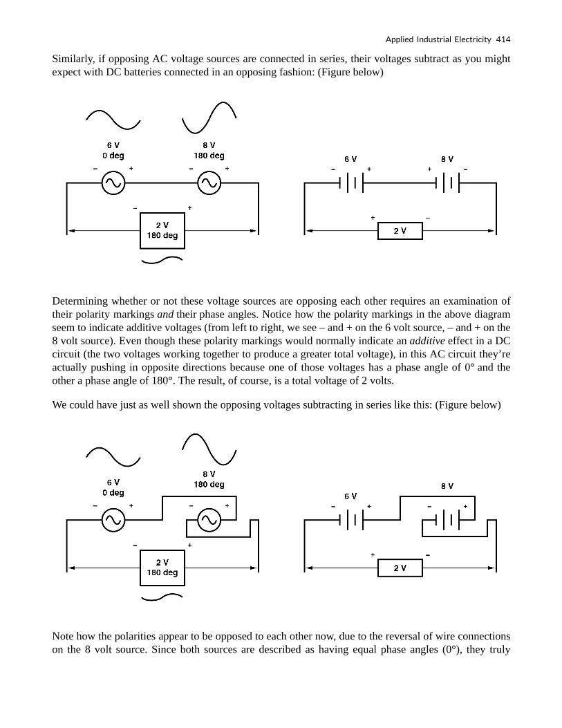
Similarly, if opposing AC voltage sources are connected in series, their voltages subtract as you might expect with DC batteries connected in an opposing fashion: (Figure below)
Determining whether or not these voltage sources are opposing each other requires an examination of their polarity markings and their phase angles. Notice how the polarity markings in the above diagram seem to indicate additive voltages (from left to right, we see – and + on the 6 volt source, – and + on the 8 volt source). Even though these polarity markings would normally indicate an additive effect in a DC circuit (the two voltages working together to produce a greater total voltage), in this AC circuit they’re actually pushing in opposite directions because one of those voltages has a phase angle of 0° and the other a phase angle of 180°. The result, of course, is a total voltage of 2 volts.
We could have just as well shown the opposing voltages subtracting in series like this: (Figure below)
Note how the polarities appear to be opposed to each other now, due to the reversal of wire connections on the 8 volt source. Since both sources are described as having equal phase angles (0°), they truly
Applied Industrial Electricity 414

are opposed to one another, and the overall effect is the same as the former scenario with “additive” polarities and differing phase angles: a total voltage of only 2 volts. (Figure below)
Just as there are two ways to express the phase of the sources, there are two ways to express the resultant their sum.
The resultant voltage can be expressed in two different ways: 2 volts at 180° with the (-) symbol on the left and the (+) symbol on the right, or 2 volts at 0° with the (+) symbol on the left and the (-) symbol
415 Tony R. Kuphaldt and John R. Haughery

on the right. A reversal of wires from an AC voltage source is the same as phase-shifting that source by 180°. (Figure below)
Example of equivalent voltage sources.
Complex Vector Addition
If vectors with uncommon angles are added, their magnitudes (lengths) add up quite differently than that of scalar magnitudes: (Figure below)
Vector magnitudes do not directly add for unequal angles.
If two AC voltages—90° out of phase—are added together by being connected in series, their voltage magnitudes do not directly add or subtract as with scalar voltages in DC. Instead, these voltage quantities are complex quantities, and just like the above vectors, which add up in a trigonometric fashion, a 6-volt source at 0° added to an 8-volt source at 90° results in 10 volts at a phase angle of 53.13°: (Figure below)
Applied Industrial Electricity 416

The 6V and 8V sources add to 10V with the help of trigonometry.
Compared to DC circuit analysis, this is very strange indeed. Note that it is possible to obtain voltmeter indications of 6 and 8 volts, respectively, across the two AC voltage sources, yet only read 10 volts for a total voltage!
There is no suitable DC analogy for what we’re seeing here with two AC voltages slightly out of phase. DC voltages can only directly aid or directly oppose, with nothing in between. With AC, two voltages can be aiding or opposing one another to any degree between fully-aiding and fully-opposing, inclusive. Without the use of vector (complex number) notation to describe AC quantities, it would be very difficult to perform mathematical calculations for AC circuit analysis.
417 Tony R. Kuphaldt and John R. Haughery

In the next section, we’ll learn how to represent vector quantities in symbolic rather than graphical form. Vector and triangle diagrams suffice to illustrate the general concept, but more precise methods of symbolism must be used if any serious calculations are to be performed on these quantities.
Review
• DC voltages can only either directly aid or directly oppose each other when
connected in series. AC voltages may aid or oppose to any degree depending on the
phase shift between them.
Polar Form and Rectangular Form Notation for Complex
Numbers
In order to work with complex numbers without drawing vectors, we first need some kind of standard mathematical notation. There are two basic forms of complex number notation: polar and rectangular.
Polar Form of a Complex Number
The polar form is where a complex number is denoted by the length (otherwise known as the magnitude, absolute value, or modulus) and the angle of its vector (usually denoted by an angle symbol that looks like this: ∠).
To use the map analogy, the polar notation for the vector from New York City to San Diego would be something like “2400 miles, southwest.” Here are two examples of vectors and their polar notations:
Applied Industrial Electricity 418
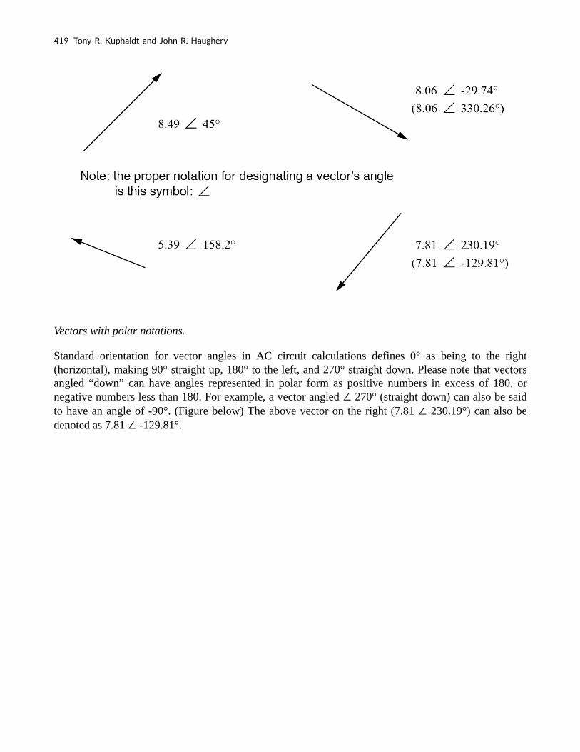
Vectors with polar notations.
Standard orientation for vector angles in AC circuit calculations defines 0° as being to the right (horizontal), making 90° straight up, 180° to the left, and 270° straight down. Please note that vectors angled “down” can have angles represented in polar form as positive numbers in excess of 180, or negative numbers less than 180. For example, a vector angled ∠ 270° (straight down) can also be said to have an angle of -90°. (Figure below) The above vector on the right (7.81 ∠ 230.19°) can also be denoted as 7.81 ∠ -129.81°.
419 Tony R. Kuphaldt and John R. Haughery

The vector compass.
Rectangular Form of a Complex Number
Rectangular form, on the other hand, is where a complex number is denoted by its respective horizontal and vertical components. In essence, the angled vector is taken to be the hypotenuse of a right triangle, described by the lengths of the adjacent and opposite sides. Rather than describing a vector’s length and direction by denoting magnitude and angle, it is described in terms of “how far left/right” and “how far up/down.”
These two-dimensional figures (horizontal and vertical) are symbolized by two numerical figures. In order to distinguish the horizontal and vertical dimensions from each other, the vertical is prefixed with
Applied Industrial Electricity 420

a lower-case “i” (in pure mathematics) or “j” (in electronics). These lower-case letters do not represent a physical variable (such as instantaneous current, also symbolized by a lower-case letter “i”), but rather are mathematical operators used to distinguish the vector’s vertical component from its horizontal component. As a complete complex number, the horizontal and vertical quantities are written as a sum: (Figure below)
In “rectangular” form the vector’s length and direction are denoted in terms of its horizontal and vertical span, the first number representing the horizontal (“real”) and the second number (with the “j” prefix) representing the vertical (“imaginary”) dimensions.
The horizontal component is referred to as the real component since that dimension is compatible with normal, scalar (“real”) numbers. The vertical component is referred to as the imaginary component since that dimension lies in a different direction, totally alien to the scale of the real numbers. (Figure below)
421 Tony R. Kuphaldt and John R. Haughery

Vector compass showing real and imaginary axes.
The “real” axis of the graph corresponds to the familiar number line we saw earlier: the one with both positive and negative values on it. The “imaginary” axis of the graph corresponds to another number line situated at 90° to the “real” one. Vectors being two-dimensional things, we must have a two-dimensional “map” upon which to express them, thus the two number lines perpendicular to each other: (Figure below)
Applied Industrial Electricity 422

Vector compass with real and imaginary (“j”) number lines.
Converting from Polar Form to Rectangular Form
Either method of notation is valid for complex numbers. The primary reason for having two methods of notation is for ease of longhand calculation, rectangular form lending itself to addition and subtraction, and polar form lending itself to multiplication and division. Conversion between the two notational forms involves simple trigonometry. To convert from polar to rectangular, find the real component by multiplying the polar magnitude by the cosine of the angle, and the imaginary component by multiplying the polar magnitude by the sine of the angle. This may be understood more readily by drawing the quantities as sides of a right triangle, the hypotenuse of the triangle representing the vector itself (its length and angle with respect to the horizontal constituting the polar form), the horizontal and vertical sides representing the “real” and “imaginary” rectangular components, respectively: (Figure below)
423 Tony R. Kuphaldt and John R. Haughery

Magnitude vector in terms of real (4) and imaginary (j3) components.
Applied Industrial Electricity 424

Converting from Rectangular Form to Polar Form
To convert from rectangular to polar, find the polar magnitude through the use of the Pythagorean Theorem (the polar magnitude is the hypotenuse of a right triangle, and the real and imaginary components are the adjacent and opposite sides, respectively), and the angle by taking the arctangent of the imaginary component divided by the real component:
Review
425 Tony R. Kuphaldt and John R. Haughery

• Polar notation denotes a complex number in terms of its vector’s length and angular
direction from the starting point. Example: fly 45 miles ∠ 203° (West by
Southwest).
• Rectangular notation denotes a complex number in terms of its horizontal and
vertical dimensions. Example: drive 41 miles West, then turn and drive 18 miles
South.
• In rectangular notation, the first quantity is the “real” component (horizontal
dimension of the vector) and the second quantity is the “imaginary” component
(vertical dimension of the vector). The imaginary component is preceded by a
lower-case “j,” sometimes called the j operator.
• Both polar and rectangular forms of notation for a complex number can be related
graphically in the form of a right triangle, with the hypotenuse representing the
vector itself (polar form: hypotenuse length = magnitude; angle with respect to
horizontal side = angle), the horizontal side representing the rectangular “real”
component, and the vertical side representing the rectangular “imaginary”
component.
Complex Number Arithmetic
Since complex numbers are legitimate mathematical entities, just like scalar numbers, they can be added, subtracted, multiplied, divided, squared, inverted, and such, just like any other kind of number. Some scientific calculators are programmed to directly perform these operations on two or more complex numbers, but these operations can also be done “by hand.” This section will show you how the basic operations are performed. It is highly recommended that you equip yourself with a scientific calculator capable of performing arithmetic functions easily on complex numbers. It will make your study of AC circuit much more pleasant than if you’re forced to do all calculations the longer way.
Addition and Subtraction of Complex Numbers in Rectangular Form
Addition and subtraction with complex numbers in rectangular form is easy. For addition, simply add up
Applied Industrial Electricity 426

the real components of the complex numbers to determine the real component of the sum, and add up the imaginary components of the complex numbers to determine the imaginary component of the sum:
When subtracting complex numbers in rectangular form, simply subtract the real component of the second complex number from the real component of the first to arrive at the real component of the difference, and subtract the imaginary component of the second complex number from the imaginary component of the first to arrive the imaginary component of the difference:
Multiplication and Division of Complex Numbers in Polar Form
For longhand multiplication and division, polar is the favored notation to work with. When multiplying complex numbers in polar form, simply multiply the polar magnitudes of the complex numbers to determine the polar magnitude of the product, and add the angles of the complex numbers to determine the angle of the product:
427 Tony R. Kuphaldt and John R. Haughery

Division of polar-form complex numbers is also easy: simply divide the polar magnitude of the first complex number by the polar magnitude of the second complex number to arrive at the polar magnitude of the quotient, and subtract the angle of the second complex number from the angle of the first complex number to arrive at the angle of the quotient:
To obtain the reciprocal, or “invert” (1/x), a complex number, simply divide the number (in polar form) into a scalar value of 1, which is nothing more than a complex number with no imaginary component (angle = 0):
Applied Industrial Electricity 428

These are the basic operations you will need to know in order to manipulate complex numbers in the analysis of AC circuits. Operations with complex numbers are by no means limited just to addition, subtraction, multiplication, division, and inversion, however. Virtually any arithmetic operation that can be done with scalar numbers can be done with complex numbers, including powers, roots, solving simultaneous equations with complex coefficients, and even trigonometric functions (although this involves a whole new perspective in trigonometry called hyperbolic functions which is well beyond the scope of this discussion). Be sure that you’re familiar with the basic arithmetic operations of addition, subtraction, multiplication, division, and inversion, and you’ll have little trouble with AC circuit analysis.
Review
• To add complex numbers in rectangular form, add the real components and add the
imaginary components. Subtraction is similar.
• To multiply complex numbers in polar form, multiply the magnitudes and add the
angles. To divide, divide the magnitudes and subtract one angle from the other.
429 Tony R. Kuphaldt and John R. Haughery
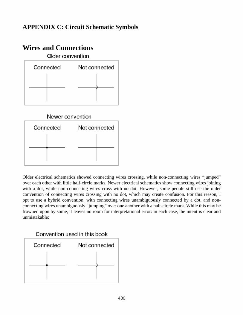
APPENDIX C: Circuit Schematic Symbols
Wires and Connections
Older electrical schematics showed connecting wires crossing, while non-connecting wires “jumped” over each other with little half-circle marks. Newer electrical schematics show connecting wires joining with a dot, while non-connecting wires cross with no dot. However, some people still use the older convention of connecting wires crossing with no dot, which may create confusion. For this reason, I opt to use a hybrid convention, with connecting wires unambiguously connected by a dot, and non-connecting wires unambiguously “jumping” over one another with a half-circle mark. While this may be frowned upon by some, it leaves no room for interpretational error: in each case, the intent is clear and unmistakable:
430

Power Sources
Resistors Types
431 Tony R. Kuphaldt and John R. Haughery

Capacitor Types
Inductors
Mutual Inductors
Applied Industrial Electricity 432

433 Tony R. Kuphaldt and John R. Haughery

Switches, Hand Actuated
Switches, Process Actuated
Applied Industrial Electricity 434

It is very important to keep in mind that the “normal” contact status of a process-actuated switch refers to its status when the process is absent and/or inactive, not “normal” in the sense of process conditions as expected during routine operation. For instance, a normally-closed low-flow detection switch installed on a coolant pipe will be maintained in the actuated state (open) when there is regular coolant flow through the pipe. If the coolant flow stops, the flow switch will go to its “normal” (un-actuated) status of closed. A limit switch is one actuated by contact with a moving machine part. An electronic limit switch senses mechanical motion but does so using light, magnetic fields, or other non-contact means.
Switches, Electrically Actuated (Relays)
435 Tony R. Kuphaldt and John R. Haughery

Connectors
Applied Industrial Electricity 436

437 Tony R. Kuphaldt and John R. Haughery

APPENDIX D: Troubleshooting - Theory And Practice
Questions to Ask Before Proceeding
• Has the system ever worked before? If yes, has anything happened to it since then that could cause the problem?
• Has this system proven itself to be prone to certain types of failure?
• How urgent is the need for repair?
• What are the safety concerns, before I start troubleshooting?
• What are the process quality concerns, before I start troubleshooting (what can I do without causing interruptions in production)?
These preliminary questions are not trivial. Indeed, they are essential to expedient and safe troubleshooting. They are especially important when the system to be trouble-shot is large, dangerous, and/or expensive. Sometimes the troubleshooter will be required to work on a system that is still in full operation (perhaps the ultimate example of this is a doctor diagnosing a live patient). Once the cause or causes are determined to a high degree of certainty, there is the step of corrective action. Correcting a system fault without significantly interrupting the operation of the system can be very challenging, and it deserves thorough planning. When there is high risk involved in taking corrective action, such as is the case with performing surgery on a patient or making repairs to an operating process in a chemical plant, it is essential for the worker(s) to plan ahead for possible trouble. One question to ask before proceeding with repairs is, “how and at what point(s) can I abort the repairs if something goes wrong?” In risky situations, it is vital to have planned “escape routes” in your corrective action, just in case things do not go as planned. A surgeon operating on a patient knows if there are any “points of no return” in such a procedure, and stops to re-check the patient before proceeding past those points. He or she also knows how to “back out” of a surgical procedure at those points if needed.
General Troubleshooting Tips
When first approaching a failed or otherwise misbehaving system, the new troubleshooter often doesn’t know where to begin. The following strategies are not exhaustive by any means, but provide the troubleshooter with a simple checklist of questions to ask in order to start isolating the problem. As for tips, these troubleshooting suggestions are not comprehensive procedures: they serve as starting points only for the troubleshooting process. An essential part of expedient troubleshooting is probability assessment, and these tips help the troubleshooter determine which possible points of failure are more or less likely than others. Final isolation of the system failure is usually determined through more specific techniques (outlined in the next section—Specific Troubleshooting Techniques).
438

Prior occurrence
If this device or process has been historically known to fail in a certain particular way, and the conditions leading to this common failure have not changed, check for this “way” first. A corollary to this troubleshooting tip is the directive to keep detailed records of failure. Ideally, a computer-based failure log is optimal, so that failures may be referenced by and correlated to a number of factors such as time, date, and environmental conditions.
Example: The car’s engine is overheating. The last two times this happened, the cause was low coolant level in the radiator.
What to do: Check the coolant level first. Of course, past history by no means guarantees the present symptoms are caused by the same problem, but since this is more likely, it makes sense to check this first. If, however, the cause of routine failure in a system has been corrected (i.e. the leak causing low coolant level in the past has been repaired), then this may not be a probable cause of trouble this time.
Recent alterations
If a system has been having problems immediately after some kind of maintenance or other change, the problems might be linked to those changes.
Example: The mechanic recently tuned my car’s engine, and now I hear a rattling noise that I didn’t hear before I took the car in for repair.
What to do: Check for something that may have been left loose by the mechanic after his or her tune-up work.
Function vs. non-function
If a system isn’t producing the desired end result, look for what it is doing correctly; in other words, identify where the problem is not, and focus your efforts elsewhere. Whatever components or subsystems necessary for the properly working parts to function are probably okay. The degree of fault can often tell you what part of it is to blame.
Example: The radio works fine on the AM band, but not on the FM band.
What to do: Eliminate from the list of possible causes, anything in the radio necessary for the AM band’s function. Whatever the source of the problem is, it is specific to the FM band and not to the AM band. This eliminates the audio amplifier, speakers, fuse, power supply, and almost all external wiring. Being able to eliminate sections of the system as possible failures reduces the scope of the problem and makes the rest of the troubleshooting procedure more efficient.
439 Tony R. Kuphaldt and John R. Haughery

Hypothesize
Based on your knowledge of how a system works, think of various kinds of failures that would cause this problem (or these phenomena) to occur, and check for those failures (starting with the most likely based on circumstances, history, or knowledge of component weaknesses).
Example: The car’s engine is overheating.
What to do: Consider possible causes for overheating, based on what you know of engine operation. Either the engine is generating too much heat, or not getting rid of the heat well enough (most likely the latter). Brainstorm some possible causes: a loose fan belt, clogged radiator, bad water pump, low coolant level, etc. Investigate each one of those possibilities before investigating alternatives.
Specific Troubleshooting Techniques
After applying some of the general troubleshooting tips to narrow the scope of a problem’s location, there are techniques useful in further isolating it. Here are a few:
Swap identical components
In a system with identical or parallel subsystems, swap components between those subsystems and see whether or not the problem moves with the swapped component. If it does, you’ve just swapped the faulty component; if it doesn’t, keep searching! This is a powerful troubleshooting method, because it gives you both a positive and a negative indication of the swapped component’s fault: when the bad part is exchanged between identical systems, the formerly broken subsystem will start working again and the formerly good subsystem will fail. I was once able to troubleshoot an elusive problem with an automotive engine ignition system using this method: I happened to have a friend with an automobile sharing the exact same model of ignition system. We swapped parts between the engines (distributor, spark plug wires, ignition coil—one at a time) until the problem moved to the other vehicle. The problem happened to be a “weak” ignition coil, and it only manifested itself under heavy load (a condition that could not be simulated in my garage). Normally, this type of problem could only be pinpointed using an ignition system analyzer (or oscilloscope) and a dynamometer to simulate loaded driving conditions. This technique, however, confirmed the source of the problem with 100% accuracy, using no diagnostic equipment whatsoever. Occasionally you may swap a component and find that the problem still exists, but has changed in some way. This tells you that the components you just swapped are somehow different (different calibration, different function), and nothing more. However, don’t dismiss this information just because it doesn’t lead you straight to the problem—look for other changes in the system as a whole as a result of the swap, and try to figure out what these changes tell you about the source of the problem. An important caveat to this technique is the possibility of causing further damage. Suppose a component has failed because of another, less conspicuous failure in the system. Swapping the failed component with a good component will cause the good component to fail as well. For example, suppose that a circuit develops a short, which “blows” the protective fuse for that circuit. The blown fuse is not evident by inspection, and you don’t have a meter to electrically test the fuse, so you decide to swap the suspect fuse with one of the same rating from a working circuit. As a result of this, the good fuse that you move
Applied Industrial Electricity 440

to the shorted circuit blows as well, leaving you with two blown fuses and two non-working circuits. At least you know for certain that the original fuse was blown, because the circuit it was moved to stopped working after the swap, but this knowledge was gained only through the loss of a good fuse and the additional “down time” of the second circuit. Another example to illustrate this caveat is the ignition system problem previously mentioned. Suppose that the “weak” ignition coil had caused the engine to backfire, damaging the muffler. If swapping ignition system components with another vehicle causes the problem to move to the other vehicle, damage may be done to the other vehicle’s muffler as well. As a general rule, the technique of swapping identical components should be used only when there is minimal chance of causing additional damage. It is an excellent technique for isolating non-destructive problems.
Example 1: You’re working on a CNC machine tool with X, Y, and Z-axis drives. The Y axis is not working, but the X and Z axes are working. All three axes share identical components (feedback encoders, servo motor drives, servo motors).
What to do: Exchange these identical components, one at a time, Y axis and either one of the working axes (X or Z), and see after each swap whether or not the problem has moved with the swap.
Example 2: A stereo system produces no sound on the left speaker, but the right speaker works just fine.
What to do: Try swapping respective components between the two channels and see if the problem changes sides, from left to right. When it does, you’ve found the defective component. For instance, you could swap the speakers between channels: if the problem moves to the other side (i.e. the same speaker that was dead before is still dead, now that its connected to the right channel cable) then you know that speaker is bad. If the problem stays on the same side (i.e. the speaker formerly silent is now producing sound after having been moved to the other side of the room and connected to the other cable), then you know the speakers are fine, and the problem must lie somewhere else (perhaps in the cable connecting the silent speaker to the amplifier, or in the amplifier itself). If the speakers have been verified as good, then you could check the cables using the same method. Swap the cables so that each one now connects to the other channel of the amplifier and to the other speaker. Again, if the problem changes sides (i.e. now the right speaker is now “dead” and the left speaker now produces sound), then the cable now connected to the right speaker must be defective. If neither swap (the speakers nor the cables) causes the problem to change sides from left to right, then the problem must lie within the amplifier (i.e. the left channel output must be “dead”).
Remove parallel components
If a system is composed of several parallel or redundant components which can be removed without crippling the whole system, start removing these components (one at a time) and see if things start to work again.
Example 1: A “star” topology communications network between several computers has failed. None of the computers are able to communicate with each other.
What to do: Try unplugging the computers, one at a time from the network, and see if the network starts working again after one of them is unplugged. If it does, then that last unplugged computer may be the one at fault (it may have been “jamming” the network by constantly outputting data or noise).
441 Tony R. Kuphaldt and John R. Haughery

Example 2: A household fuse keeps blowing (or the breaker keeps tripping open) after a short amount of time.
What to do: Unplug appliances from that circuit until the fuse or breaker quits interrupting the circuit. If you can eliminate the problem by unplugging a single appliance, then that appliance might be defective. If you find that unplugging almost any appliance solves the problem, then the circuit may simply be overloaded by too many appliances, neither of them defective.
Divide system into sections and test those sections
In a system with multiple sections or stages, carefully measure the variables going in and out of each stage until you find a stage where things don’t look right.
Example 1: A radio is not working (producing no sound at the speaker))
What to do: Divide the circuitry into stages: tuning stage, mixing stages, amplifier stage, all the way through to the speaker(s). Measure signals at test points between these stages and tell whether or not a stage is working properly.
Example 2: An analog summer circuit is not functioning properly.
What to do: I would test the passive averager network (the three resistors at the lower-left corner of the schematic) to see that the proper (averaged) voltage was seen at the noninverting input of the op-amp. I would then measure the voltage at the inverting input to see if it was the same as at the noninverting input (or, alternatively, measure the voltage difference between the two inputs of the op-amp, as it should be zero). Continue testing sections of the circuit (or just test points within the circuit) to see if you measure the expected voltages and currents.
Applied Industrial Electricity 442

Simplify and rebuild
Closely related to the strategy of dividing a system into sections, this is actually a design and fabrication technique useful for new circuits, machines, or systems. It’s always easier begin the design and construction process in little steps, leading to larger and larger steps, rather than to build the whole thing at once and try to troubleshoot it as a whole. Suppose that someone were building a custom automobile. He or she would be foolish to bolt all the parts together without checking and testing components and subsystems as they went along, expecting everything to work perfectly after its all assembled. Ideally, the builder would check the proper operation of components along the way through the construction process: start and tune the engine before its connected to the drivetrain, check for wiring problems before all the cover panels are put in place, check the brake system in the driveway before taking it out on the road, etc. Countless times I’ve witnessed students build a complex experimental circuit and have trouble getting it to work because they didn’t stop to check things along the way: test all resistors before plugging them into place, make sure the power supply is regulating voltage adequately before trying to power anything with it, etc. It is human nature to rush to completion of a project, thinking that such checks are a waste of valuable time. However, more time will be wasted in troubleshooting a malfunctioning circuit than would be spent checking the operation of subsystems throughout the process of construction. Take the example of the analog summer circuit in the previous section for example: what if it wasn’t working properly? How would you simplify it and test it in stages? Well, you could reconnect the op-amp as a basic comparator and see if its responsive to differential input voltages, and/or connect it as a voltage follower (buffer) and see if it outputs the same analog voltage as what is input. If it doesn’t perform these simple functions, it will never perform its function in the summer circuit! By stripping away the complexity of the summer circuit, paring it down to an (almost) bare op-amp, you can test that component’s functionality and then build from there (add resistor feedback and check for voltage amplification, then add input resistors and check for voltage summing), checking for expected results along the way.
Trap a signal
Set up instrumentation (such as a datalogger, chart recorder, or multimeter set on “record” mode) to monitor a signal over a period of time. This is especially helpful when tracking down intermittent problems, which have a way of showing up the moment you’ve turned your back and walked away. This may be essential for proving what happens first in a fast-acting system. Many fast systems (especially shutdown “trip” systems) have a “first out” monitoring capability to provide this kind of data.
Example #1: A turbine control system shuts automatically in response to an abnormal condition. By the time a technician arrives at the scene to survey the turbine’s condition, however, everything is in a “down” state and its impossible to tell what signal or condition was responsible for the initial shutdown, as all operating parameters are now “abnormal.”
What to do: One technician I knew used a videocamera to record the turbine control panel, so he could see what happened (by indications on the gauges) first in an automatic-shutdown event. Simply by looking at the panel after the fact, there was no way to tell which signal shut the turbine down, but the videotape playback would show what happened in sequence, down to a frame-by-frame time resolution.
443 Tony R. Kuphaldt and John R. Haughery

Example #2: An alarm system is falsely triggering, and you suspect it may be due to a specific wire connection going bad. Unfortunately, the problem never manifests itself while you’re watching it!
What to do: Many modern digital multimeters are equipped with “record” settings, whereby they can monitor a voltage, current, or resistance over time and note whether that measurement deviates substantially from a regular value. This is an invaluable tool for use in “intermittent” electronic system failures.
Likely Failures in Proven Systems
The following problems are arranged in order from most likely to least likely, top to bottom. This order has been determined largely from personal experience troubleshooting electrical and electronic problems in automotive, industrial, and home applications. This order also assumes a circuit or system that has been proven to function as designed and has failed after substantial operation time. Problems experienced in newly assembled circuits and systems do not necessarily exhibit the same probabilities of occurrence.
Operator error
A frequent cause of system failure is error on the part of those human beings operating it. This cause of trouble is placed at the top of the list, but of course, the actual likelihood depends largely on the particular individuals responsible for operation. When operator error is the cause of a failure, it is unlikely that it will be admitted prior to investigation. I do not mean to suggest that operators are incompetent and irresponsible—quite the contrary: these people are often your best teachers for learning system function and obtaining a history of failure—but the reality of human error cannot be overlooked. A positive attitude coupled with good interpersonal skills on the part of the troubleshooter goes a long way in troubleshooting when human error is the root cause of failure.
Bad wire connections
As incredible as this may sound to the new student of electronics, a high percentage of electrical and electronic system problems are caused by a very simple source of trouble: poor (i.e. open or shorted) wire connections. This is especially true when the environment is hostile, including such factors as high vibration and/or a corrosive atmosphere. Connection points found in any variety of plug-and-socket connector, terminal strip, or splice are at the greatest risk for failure. The category of “connections” also includes mechanical switch contacts, which can be thought of as a high-cycle connector. Improper wire termination lugs (such as a compression-style connector crimped on the end of a solid wire—a definite faux pas) can cause high-resistance connections after a period of trouble-free service. It should be noted that connections in low-voltage systems tend to be far more troublesome than connections in high-voltage systems. The main reason for this is the effect of arcing across a discontinuity (circuit break) in higher-voltage systems tends to blast away insulating layers of dirt and corrosion, and may even weld the two ends together if sustained long enough.
Applied Industrial Electricity 444

Low-voltage systems tend not to generate such vigorous arcing across the gap of a circuit break, and also tend to be more sensitive to additional resistance in the circuit. Mechanical switch contacts used in low-voltage systems benefit from having the recommended minimum wetting current conducted through them to promote a healthy amount of arcing upon opening, even if this level of current is not necessary for the operation of other circuit components. Although open failures tend to more common than shorted failures, “shorts” still constitute a substantial percentage of wiring failure modes. Many shorts are caused by degradation of wire insulation. This, again, is especially true when the environment is hostile, including such factors as high vibration, high heat, high humidity, or high voltage. It is rare to find a mechanical switch contact that is failed shorted, except in the case of high-current contacts where contact “welding” may occur in over current conditions. Shorts may also be caused by conductive build up across terminal strip sections or the backs of printed circuit boards. A common case of shorted wiring is the ground fault, where a conductor accidentally makes contact with either earth or chassis ground. This may change the voltage(s) present between other conductors in the circuit and ground, thereby causing bizarre system malfunctions and/or personnel hazard.
Power supply problems
These generally consist of tripped overcurrent protection devices or damage due to overheating. Although power supply circuitry is usually less complex than the circuitry being powered and therefore should figure to be less prone to failure on that basis alone, it generally handles more power than any other portion of the system and therefore must deal with greater voltages and/or currents. Also, because of its relative design simplicity, a system’s power supply may not receive the engineering attention it deserves, most of the engineering focus devoted to more glamorous parts of the system.
Active components
Active components (amplification devices) tend to fail with greater regularity than passive (non-amplifying) devices, due to their greater complexity and tendency to amplify overvoltage/overcurrent conditions. Semiconductor devices are notoriously prone to failure due to electrical transient (voltage/current surge) overloading and thermal (heat) overloading. Electron tube devices are far more resistant to both of these failure modes but are generally more prone to mechanical failures due to their fragile construction.
Passive components
Non-amplifying components are the most rugged of all, their relative simplicity granting them a statistical advantage over active devices. The following list gives an approximate relation of failure probabilities (again, top being the most likely and bottom being the least likely):
• Capacitors (shorted), especially electrolytic capacitors. The paste electrolyte tends to lose moisture with age, leading to failure. Thin dielectric layers may be punctured by overvoltage transients.
445 Tony R. Kuphaldt and John R. Haughery

• Diodes open (rectifying diodes) or shorted (Zener diodes).
• Inductor and transformer windings open or shorted to conductive core. Failures related to overheating (insulation breakdown) are easily detected by smell.
• Resistors open, almost never shorted. Usually, this is due to overcurrent heating, although it is less frequently caused by overvoltage transient (arc-over) or physical damage (vibration or impact). Resistors may also change resistance value if overheated!
Likely Failures in Unproven Systems
“All men are liable to error;” —John Locke
Whereas the last section deals with component failures in systems that have been successfully operating for some time, this section concentrates on the problems plaguing brand-new systems. In this case, failure modes are generally not of the aging kind but are related to mistakes in design and assembly caused by human beings.
Wiring problems
In this case, bad connections are usually due to assembly error, such as connection to the wrong point or poor connector fabrication. Shorted failures are also seen, but usually, involve misconnections (conductors inadvertently attached to grounding points) or wires pinched under box covers. Another wiring-related problem seen in new systems is that of electrostatic or electromagnetic interference between different circuits by way of close wiring proximity. This kind of problem is easily created by routing sets of wires too close to each other (especially routing signal cables close to power conductors) and tends to be very difficult to identify and locate with test equipment.
Power supply problems
Blown fuses and tripped circuit breakers are likely sources of trouble, especially if the project in question is an addition to an already-functioning system. Loads may be larger than expected, resulting in overloading and subsequent failure of power supplies.
Defective components
In the case of a newly-assembled system, component fault probabilities are not as predictable as in the case of an operating system that fails with age. Any type of component—active or passive—may be found defective or of imprecise value “out of the box” with roughly equal probability, barring any specific sensitivities in shipping (i.e fragile vacuum tubes or electrostatically sensitive semiconductor components). Moreover, these types of failures are not always as easy to identify by sight or smell as an age- or transient-induced failure.
Applied Industrial Electricity 446

Improper system configuration
Increasingly seen in large systems using microprocessor-based components, “programming” issues can still plague non-microprocessor systems in the form of incorrect time-delay relay settings, limit switch calibrations, and drum switch sequences. Complex components having configuration “jumpers” or switches to control behavior may not be “programmed” properly. Components may be used in a new system outside of their tolerable ranges. Resistors, for example, with too low of power ratings, of too great of tolerance, may have been installed. Sensors, instruments, and controlling mechanisms may be uncalibrated, or calibrated to the wrong ranges.
Design error
Perhaps the most difficult to pinpoint and the slowest to be recognized (especially by the chief designer) is the problem of design error, where the system fails to function simply because it cannot function as designed. This may be as trivial as the designer specifying the wrong components in a system, or as fundamental as a system not working due to the designer’s improper knowledge of physics. I once saw a turbine control system installed that used a low-pressure switch on the lubrication oil tubing to shut down the turbine if oil pressure dropped to an insufficient level. The oil pressure for lubrication was supplied by an oil pump turned by the turbine. When installed, the turbine refused to start. Why? Because when it was stopped, the oil pump was not turning, thus there was no oil pressure to lubricate the turbine. The low-oil-pressure switch detected this condition and the control system maintained the turbine in shutdown mode, preventing it from starting. This is a classic example of a design flaw, and it could only be corrected by a change in the system logic. While most design flaws manifest themselves early in the operational life of the system, some remain hidden until just the right conditions exist to trigger the fault. These types of flaws are the most difficult to uncover, as the troubleshooter usually overlooks the possibility of design error due to the fact that the system is assumed to be “proven.” The example of the turbine lubrication system was a design flaw impossible to ignore on start-up. An example of a “hidden” design flaw might be a faulty emergency coolant system for a machine, designed to remain inactive until certain abnormal conditions are reached—conditions which might never be experienced in the life of the system.
Potential Pitfalls
Fallacious reasoning and poor interpersonal relations account for more failed or belabored troubleshooting efforts than any other impediments. With this in mind, the aspiring troubleshooter needs to be familiar with a few common troubleshooting mistakes.
Trusting that a brand-new component will always be good. While it is generally true that a new component will be in good condition, it is not always true. It is also possible that a component has been mislabeled and may have the wrong value (usually this mislabeling is a mistake made at the point of distribution or warehousing and not at the manufacturer, but again, not always!).
Not periodically checking your test equipment. This is especially true with battery-powered meters, as weak batteries may give spurious readings. When using meters to safety-check for dangerous voltage,
447 Tony R. Kuphaldt and John R. Haughery

remember to test the meter on a known source of voltage both before and after checking the circuit to be serviced, to make sure the meter is in proper operating condition.
Assuming there is only one failure to account for the problem. Single-failure system problems are ideal for troubleshooting, but sometimes failures come in multiple numbers. In some instances, the failure of one component may lead to a system condition that damages other components. Sometimes a component in marginal condition goes undetected for a long time, then when another component fails the system suffers from problems with both components.
Mistaking coincidence for causality. Just because two events occurred at nearly the same time does not necessarily mean one event caused the other! They may be both consequences of a common cause, or they may be totally unrelated! If possible, try to duplicate the same condition suspected to be the cause and see if the event suspected to be the coincidence happens again. If not, then there is either no causal relationship as assumed. This may mean there is no causal relationship between the two events whatsoever, or that there is a causal relationship, but just not the one you expected.
Self-induced blindness. After a long effort at troubleshooting a difficult problem, you may become tired and begin to overlook crucial clues to the problem. Take a break and let someone else look at it for a while. You will be amazed at what a difference this can make. On the other hand, it is generally a bad idea to solicit help at the start of the troubleshooting process. Effective troubleshooting involves complex, multi-level thinking, which is not easily communicated with others. More often than not, “team troubleshooting” takes more time and causes more frustration than doing it yourself. An exception to this rule is when the knowledge of the troubleshooters is complementary: for example, a technician who knows electronics but not machine operation teamed with an operator who knows machine function but not electronics.
Failing to question the troubleshooting work of others on the same job. This may sound rather cynical and misanthropic, but it is sound scientific practice. Because it is easy to overlook important details, troubleshooting data received from another troubleshooter should be personally verified before proceeding. This is a common situation when troubleshooters “change shifts” and a technician takes over for another technician who is leaving before the job is done. It is important to exchange information, but do not assume the prior technician checked everything they said they did or checked it perfectly. I’ve been hindered in my troubleshooting efforts on many occasions by failing to verify what someone else told me they checked.
Being pressured to “hurry up.” When an important system fails, there will be pressure from other people to fix the problem as quickly as possible. As they say in business, “time is money.” Having been on the receiving end of this pressure many times, I can understand the need for expedience. However, in many cases, there is a higher priority: caution. If the system in question harbors great danger to life and limb, the pressure to “hurry up” may result in injury or death. At the very least, hasty repairs may result in further damage when the system is restarted. Most failures can be recovered or at least temporarily repaired in short time if approached intelligently. Improper “fixes” resulting in haste often lead to damage that cannot be recovered in short time, if ever. If the potential for greater harm is present, the troubleshooter needs to politely address the pressure received from others, and maintain their perspective in the midst of chaos. Interpersonal skills are just as important in this realm as technical ability!
Finger-pointing. It is all too easy to blame a problem on someone else, for reasons of ignorance,
Applied Industrial Electricity 448

pride, laziness, or some other unfortunate facet of human nature. When the responsibility for system maintenance is divided into departments or work crews, troubleshooting efforts are often hindered by blame cast between groups. “It’s a mechanical problem . . . it’s an electrical problem . . . it’s an instrument problem . . .” ad infinitum, ad nauseum, is all too common in the workplace. I have found that a positive attitude does more to quench the fires of the blame than anything else. On one particular job, I was summoned to fix a problem in a hydraulic system assumed to be related to the electronic metering and controls. My troubleshooting isolated the source of trouble to a faulty control valve, which was the domain of the millwright (mechanical) crew. I knew that the millwright on shift was a contentious person, so I expected trouble if I simply passed the problem on to his department. Instead, I politely explained to him and his supervisor the nature of the problem as well as a brief synopsis of my reasoning, then proceeded to help him replace the faulty valve, even though it wasn’t “my” responsibility to do so. As a result, the problem was fixed very quickly, and I gained the respect of the millwright.
449 Tony R. Kuphaldt and John R. Haughery