applied econometrics - lecture 4 - nathaniel higgins€¦ · · 2011-11-01applied econometrics...
TRANSCRIPT
HomeworkReview from last time
OverviewPractical concerns
Examples
Applied EconometricsLecture 4
Nathaniel Higgins
ERS and JHU
27 September 2010
Nathaniel Higgins AE Lecture 4

HomeworkReview from last time
OverviewPractical concerns
Examples
Outline
1 Homework (brief)2 Review from last time
Example of IV (reverse causality flavor)3 Necessary conditions for IV4 How to test for exogeneity (one method)5 Weak instruments6 IV discussion7 Homework start (if time)
Nathaniel Higgins AE Lecture 4

HomeworkReview from last time
OverviewPractical concerns
Examples
Homework answers
A few of you tried using MataNeed to use a specialized syntax if you want it to workSee http://www.stata.com/help.cgi?m1_ado if you want toknow how to do itMata works great with a do-file — a bit different withado-files
Some of you used vecaccum and/or matrix accumMake sure you know what this doesIt is a convenient shortcut, but sometimes shortcuts makethe code less transparent
Using mkmat is the most straightforward way to do thisRegardless of how you manipulated matrices, most of youappear to have some trouble with how to handle inputs
Nathaniel Higgins AE Lecture 4

HomeworkReview from last time
OverviewPractical concerns
Examples
Homework answers
Several ways to get the job doneEasiest (for me to understand) is positional inputsAlso, using gettokens works very wellSee olsNH.ado, foo.ado, olsNH2.ado, and ereturn
Nathaniel Higgins AE Lecture 4
HomeworkReview from last time
OverviewPractical concerns
Examples
Instrumental variablesTry it
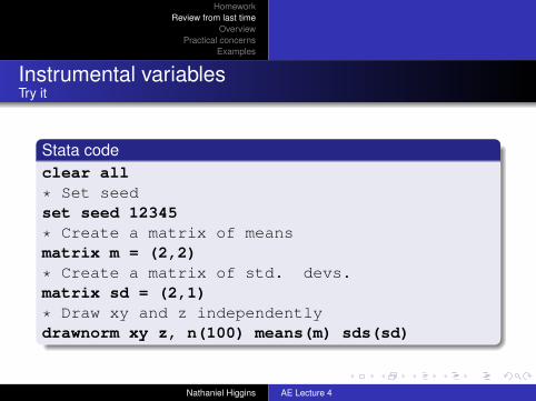
Stata codeclear all
* Set seedset seed 12345
* Create a matrix of meansmatrix m = (2,2)
* Create a matrix of std. devs.matrix sd = (2,1)
* Draw xy and z independentlydrawnorm xy z, n(100) means(m) sds(sd)
Nathaniel Higgins AE Lecture 4
HomeworkReview from last time
OverviewPractical concerns
Examples
Instrumental variablesTry it
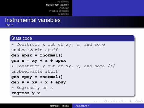
Stata code* Construct x out of xy, z, and someunobservable stuffgen epsx = rnormal()gen x = xy + z + epsx
* Construct y out of xy, x, and some ///unobservable stuffgen epsy = rnormal()gen y = xy + x + epsy
* Regress y on xregress y x
Nathaniel Higgins AE Lecture 4
HomeworkReview from last time
OverviewPractical concerns
Examples
Instrumental variablesTry it
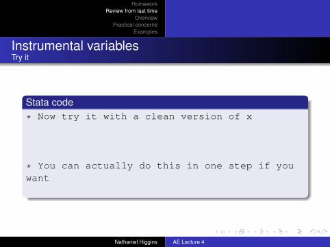
Stata code* Now try it with a clean version of x
regress x zpredict xcleanregress y xclean
* You can actually do this in one step if youwant
ivregress 2sls y (x = z)
Nathaniel Higgins AE Lecture 4

HomeworkReview from last time
OverviewPractical concerns
Examples
Instrumental variablesTry it
Stata code* Now try it with a clean version of xregress x zpredict xcleanregress y xclean
* You can actually do this in one step if youwant
ivregress 2sls y (x = z)
Nathaniel Higgins AE Lecture 4

HomeworkReview from last time
OverviewPractical concerns
Examples
Instrumental variablesTry it
Stata code* Now try it with a clean version of xregress x zpredict xcleanregress y xclean
* You can actually do this in one step if youwantivregress 2sls y (x = z)
Nathaniel Higgins AE Lecture 4

HomeworkReview from last time
OverviewPractical concerns
Examples
IVReview from last time
IV is a well-used technique to solve the general problem ofendogeneityEndogeneity is: correlation between a regressor and theerror term (the unobservables)Why is endogeneity a problem?
Think of all endogeneity problems like an omitted variablesproblemThe error (the unobservables) are always “omitted”It’s no problem if an omitted variable is uncorrelated with anincluded regressor. But if an omitted variable is correlatedwith an included regressor, we then ascribe someexplanatory variation to the regressor that we should nothave.
Nathaniel Higgins AE Lecture 4
HomeworkReview from last time
OverviewPractical concerns
Examples
IVOverview
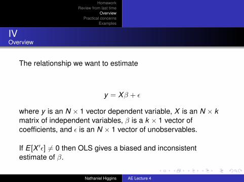
The relationship we want to estimate
y = Xβ + ε
where y is an N × 1 vector dependent variable, X is an N × kmatrix of independent variables, β is a k × 1 vector ofcoefficients, and ε is an N × 1 vector of unobservables.
If E [X ′ε] 6= 0 then OLS gives a biased and inconsistentestimate of β.
Nathaniel Higgins AE Lecture 4
HomeworkReview from last time
OverviewPractical concerns
Examples
IVOverview
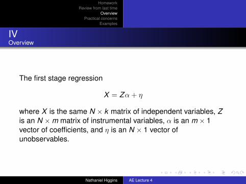
The first stage regression
X = Zα+ η
where X is the same N × k matrix of independent variables, Zis an N ×m matrix of instrumental variables, α is an m × 1vector of coefficients, and η is an N × 1 vector ofunobservables.
Nathaniel Higgins AE Lecture 4

HomeworkReview from last time
OverviewPractical concerns
Examples
IVThe procedure
There are a few (roughly) equivalent ways to calculate aninstrumental variables estimatorThe one that’s easiest and most intuitive to understand is2SLS
1 Run a regression of X on Z (this is called the first stageregression)
2 Obtain X̂ , the predicted X ’s (or the “clean” X ’s)3 Use these clean X ’s as the independent variables in the
second stage regression:
y = X̂β + ε
If the variables Z were good instruments, then the OLSestimate of y on X̂ produces consistent estimates of β
Nathaniel Higgins AE Lecture 4
HomeworkReview from last time
OverviewPractical concerns
Examples
IVAn alternative procedure
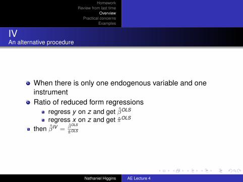
When there is only one endogenous variable and oneinstrumentRatio of reduced form regressions
regress y on z and get β̂OLS
regress x on z and get π̂OLS
then β̂IV = β̂OLS
π̂OLS
Nathaniel Higgins AE Lecture 4
HomeworkReview from last time
OverviewPractical concerns
Examples
IVThe necessary conditions
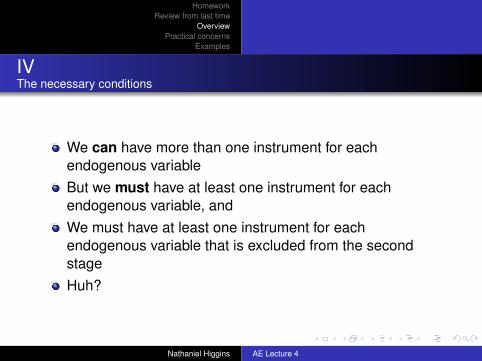
We can have more than one instrument for eachendogenous variableBut we must have at least one instrument for eachendogenous variable, andWe must have at least one instrument for eachendogenous variable that is excluded from the secondstageHuh?
Nathaniel Higgins AE Lecture 4

HomeworkReview from last time
OverviewPractical concerns
Examples
IVThe necessary conditions
Think of the first stage just like any other regression — youcan have as many Z variables as you think sensibly predictXAnd you can include some of these Z ’s in the second stageregression too, if you think that the Z ’s cause y as wellBut you must have at least one Z variable for everyendogenous X variable that you exclude from the secondstageThis is called an exclusion restrictionYou can have as many independent first-stage equationsas you want, or you can use the same instruments for eachendogenous variable, but you must have at least the samenumber of instruments as endogenous variables
Nathaniel Higgins AE Lecture 4
HomeworkReview from last time
OverviewPractical concerns
Examples
IVThe necessary condtions
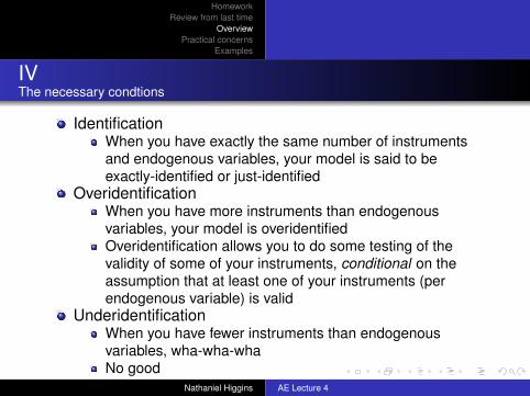
IdentificationWhen you have exactly the same number of instrumentsand endogenous variables, your model is said to beexactly-identified or just-identified
OveridentificationWhen you have more instruments than endogenousvariables, your model is overidentifiedOveridentification allows you to do some testing of thevalidity of some of your instruments, conditional on theassumption that at least one of your instruments (perendogenous variable) is valid
UnderidentificationWhen you have fewer instruments than endogenousvariables, wha-wha-whaNo good
Nathaniel Higgins AE Lecture 4
HomeworkReview from last time
OverviewPractical concerns
Examples
IVThe necessary conditions
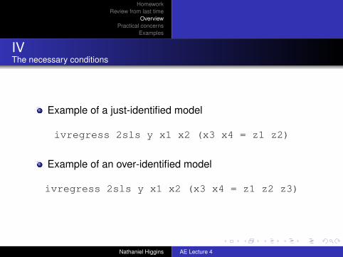
Example of a just-identified model
ivregress 2sls y x1 x2 (x3 x4 = z1 z2)
Example of an over-identified model
ivregress 2sls y x1 x2 (x3 x4 = z1 z2 z3)
Nathaniel Higgins AE Lecture 4

HomeworkReview from last time
OverviewPractical concerns
Examples
IVTesting for endogeneity
You can test for exogeneity of your regressorsBe careful interpreting the results of this test — results arealways based on the assumptions you make!The exogeneity test is one example of a general test calleda Hausman testHausman tests are based on the comparison of twoestimators:
1 One that is consistent2 One that is most efficient under the null hypothesis
Nathaniel Higgins AE Lecture 4
HomeworkReview from last time
OverviewPractical concerns
Examples
IVTesting for endogeneity
The basic idea is simple:Compare the more efficient estimator to the consistentestimatorBecause the consistent estimator is, well, consistent, weknow that it should provide a good point estimate, even ifthe standard errors are highIf the more efficient estimator is pretty close (statisticallyspeaking) to the consistent estimator, then we are confidentin the efficient estimator and we use that
Nathaniel Higgins AE Lecture 4

HomeworkReview from last time
OverviewPractical concerns
Examples
IVTesting for endogeneity
In the context of testing exogeneity, we compare the OLSestimate to the IV estimateNull hypothesis is that the regressor of interest isexogenousUnder the null, which is more efficient, IV or OLS?
OLSBut IV is consistent if the null failsYou can think of it this way:
If the null is false (the regressor is endogenous) then OLSshould be affected, but IV should still be consistentSo if the two regressors are much different, then we rejectthe null (we say that the regressor is endogenous)
Nathaniel Higgins AE Lecture 4

HomeworkReview from last time
OverviewPractical concerns
Examples
IVTesting for endogeneity
In the context of testing exogeneity, we compare the OLSestimate to the IV estimateNull hypothesis is that the regressor of interest isexogenousUnder the null, which is more efficient, IV or OLS?OLSBut IV is consistent if the null failsYou can think of it this way:
If the null is false (the regressor is endogenous) then OLSshould be affected, but IV should still be consistentSo if the two regressors are much different, then we rejectthe null (we say that the regressor is endogenous)
Nathaniel Higgins AE Lecture 4
HomeworkReview from last time
OverviewPractical concerns
Examples
IVTesting for endogeneity
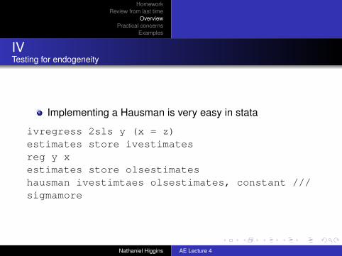
Implementing a Hausman is very easy in stata
ivregress 2sls y (x = z)estimates store ivestimatesreg y xestimates store olsestimateshausman ivestimtaes olsestimates, constant ///sigmamore
Nathaniel Higgins AE Lecture 4
HomeworkReview from last time
OverviewPractical concerns
Examples
IVTesting for endogeneity
The Hausman test is very commonly used and it isrelatively easy to interpretThere are other tests that are robustThe intuition for the Durbin-Wu-Hausman test is not quiteas straightforward, but it actually isn’t all that tough to run,and the interpretation is the same as the Hausman test
ivregress 2sls y (x = z)estat endogenous
If the p-value is small, then we reject the null of exogeneity
Nathaniel Higgins AE Lecture 4
HomeworkReview from last time
OverviewPractical concerns
Examples
IVTesting overidentification
When you have an overidentified model, you have moreinstruments than you needWhen this is the case, under the assumption that at leastone of your instruments is valid, you can test the validity ofthe others (the “overidentifying” restrictions)
ivregress gmm y (x = z1 z2)estat overid
The null hypothesis is that the restrictions are valid, so ahigh p-value does not reject the nullIf you reject the null, some of your instruments are said tobe invalid
Nathaniel Higgins AE Lecture 4
HomeworkReview from last time
OverviewPractical concerns
Examples
IVWhat makes a “good” instrument?
It is possible to have a valid instrument that isn’t all thatgoodAn instrument can be valid as long as it is at least a little bitcorrelated with x and arguably not correlated with ε
Just because an instrument is valid, does not mean it isgoodA good instrument . . .
is highly correlated with x and definitely not correlated with ε“highly” correlated doesn’t mean much in practice, so whatdo people do?
Nathaniel Higgins AE Lecture 4
HomeworkReview from last time
OverviewPractical concerns
Examples
IVWhat makes a “good” instrument?
Normal procedureRun the first stage regression
x = zα+ η
Check the F-stat on the first stage regressionF-stat should be at least 10Caution: This is a rough guideline — it has no real meaning
Nathaniel Higgins AE Lecture 4
HomeworkReview from last time
OverviewPractical concerns
Examples
IVWhat makes a “good” instrument?
So what happens with an F-stat less than 10?You might have a weak instrumentAn F-stat less than 10 doesn’t define a weak instrument,but it’s an indicationProblem with weak instruments:
IV estimator might be biasedIV estimator will certainly have a very high standard errorBottom line: you might have a crap estimate of β
Nathaniel Higgins AE Lecture 4
HomeworkReview from last time
OverviewPractical concerns
Examples
IVSample sizes
IV should only be used in large samplesIf you have to use IV and you have a relatively small dset,try LIML (Levitt (1997))Sometimes, with small samples and weak instruments, youmay notice a precipitous drop in precision from OLS to IV
Unfortunately, all you can do is get more data or betterinstruments
Nathaniel Higgins AE Lecture 4
HomeworkReview from last time
OverviewPractical concerns
Examples
IVSample sizes
More instruments are better in infinite (OK, really big)samplesMore instruments can make small sample bias worseYou might be forced to choose a “best” instrument, which isreally the instrument with the most explanatory power(most correlation with y that is not also explained by otheravailable instruments
Nathaniel Higgins AE Lecture 4
HomeworkReview from last time
OverviewPractical concerns
Examples
IVPractical advice
Run the first stage regression and report itRun the reduced-form regression and check that yourinstruments appear to influence your dependent variableTry LIML if you have small samplesReport all the models you try (OLS, 2SLS, LIML) andcompare what you know about them to tell a storyUse robust standard errors to make sure that you are beingconservative with your data (use option , vce(robust)after your regular command:ivregress 2sls y (x = z), vce(robust)
Nathaniel Higgins AE Lecture 4

HomeworkReview from last time
OverviewPractical concerns
Examples
IVPractical advice
Use the first option when running ivregress in stataThis option will give you info on the first stage regression
Doing this has two benefitsFirst, if you mistakenly ran a regression you didn’t mean to,info. in the first stage should reveal that to youSecond, the first stage automatically includes diagnostictests
Nathaniel Higgins AE Lecture 4
HomeworkReview from last time
OverviewPractical concerns
Examples
Levitt (1997)
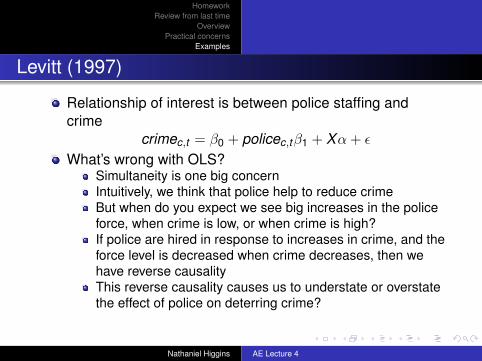
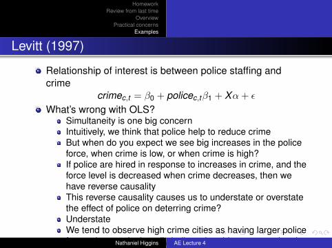
Relationship of interest is between police staffing andcrime
crimec,t = β0 + policec,tβ1 + Xα+ ε
What’s wrong with OLS?Simultaneity is one big concernIntuitively, we think that police help to reduce crimeBut when do you expect we see big increases in the policeforce, when crime is low, or when crime is high?If police are hired in response to increases in crime, and theforce level is decreased when crime decreases, then wehave reverse causalityThis reverse causality causes us to understate or overstatethe effect of police on deterring crime?
UnderstateWe tend to observe high crime cities as having larger policeforces, but we don’t really believe that this cross-sectionalcomparison is validWe don’t believe that if we reduced the number of police inDetroit that crime would fall, even though Detroit has bothmore police offers per capita and more crime per capitathan Omaha
Nathaniel Higgins AE Lecture 4
HomeworkReview from last time
OverviewPractical concerns
Examples
Levitt (1997)
Relationship of interest is between police staffing andcrime
crimec,t = β0 + policec,tβ1 + Xα+ ε
What’s wrong with OLS?Simultaneity is one big concernIntuitively, we think that police help to reduce crimeBut when do you expect we see big increases in the policeforce, when crime is low, or when crime is high?If police are hired in response to increases in crime, and theforce level is decreased when crime decreases, then wehave reverse causalityThis reverse causality causes us to understate or overstatethe effect of police on deterring crime?UnderstateWe tend to observe high crime cities as having larger policeforces, but we don’t really believe that this cross-sectionalcomparison is validWe don’t believe that if we reduced the number of police inDetroit that crime would fall, even though Detroit has bothmore police offers per capita and more crime per capitathan Omaha
Nathaniel Higgins AE Lecture 4

HomeworkReview from last time
OverviewPractical concerns
Examples
Levitt 1997
Use data from 59 cities from 1970 to 1992(Note: this is “panel data”)Observations are annualCrime and police force size are taken from Uniform CrimeReports (FBI)Uniform Crime Reports record:
Murder and nonnegligent manslaughterForcible rapeAssaultRobberyBurglaryLarcenyVehicle theft
Nathaniel Higgins AE Lecture 4
HomeworkReview from last time
OverviewPractical concerns
Examples
Levitt 1997
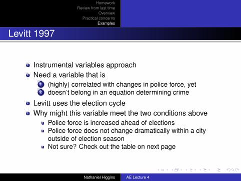
Instrumental variables approachNeed a variable that is
1 (highly) correlated with changes in police force, yet2 doesn’t belong in an equation determining crime
Levitt uses the election cycleWhy might this variable meet the two conditions above
Police force is increased ahead of electionsPolice force does not change dramatically within a cityoutside of election seasonNot sure? Check out the table on next page
Nathaniel Higgins AE Lecture 4

HomeworkReview from last time
OverviewPractical concerns
Examples
Levitt 1997
VOL. 87 NO. 3 LEVIIT: USING ELECTORAL CYCLES IN POLICE HIRING 275
While the motives of incumbent governors are likely to be similar to those of incumbent mayors, the mechanism by which governors might affect levels of city police staffing is less straightforward since the state government does not typically directly hire local police. State governments do, however, provide sub- stantial local aid to city governments (repre- senting more than 20 percent of general revenues for large cities), as well as a more limited amount of intergovernmental grants tied specifically to local law enforcement. Tim Besley and Anne Case (1995) document gu- bernatorial election cycles for a range of fiscal variables. Although intergovernmental grants is not among the categories Besley and Case examine, the existence of cycles in intergov- ernmental grants would not be implausible in light of their other results.
Empirically, changes in the size of police forces do, indeed, tend to mirror the political cycle in large cities. A simple comparison of the mean percentage change in the number of police officers per capita in the sample across election and nonelection years, presented be- low, shows that the number of sworn officers grows by approximately 2 percent on average in both gubernatorial and mayoral election years, but is completely flat in nonelection years (standard deviations in parentheses):10
Mayoral Gubernatorial election election year year No election
(N= 302) (N= 391) (N= 621)
zln Sworn 0.021 0.020 0.000 police (0.006) (0.007) (0.006) officers per capita
The propensity to increase police forces around elections also emerges when the data is analyzed on a year-by-year basis. Figure 2 pro- vides a comparison of increases in sworn officers for cities with and without elections in a given year (either mayoral or gubernatorial). While
there is substantial year-to-year variability in the average change in the number of sworn officers, cities with elections in the current year exhibit higher rates of increase (or smaller decreases) in 20 of the 23 years. If changes in sworn officers are independent across cities and are unrelated to the timing of elections, the likelihood that cit- ies holding elections would have higher rates of increase in 20 or more of 23 cases is less than one in 4,000."
Another way of examining the robustness of the relationship between sworn officers and elections is to analyze the data on a city-by- city basis. A full list of cities, along with in- formation on mean changes in sworn officers per capita in gubernatorial, mayoral, and non- election years, is provided in the Appendix. Excluding Washington, DC, which does not have gubernatorial elections, 43 of the 58 cit- ies in the sample have higher mean rates of increase in gubernatorial election years com- pared to years in which there are neither gu- bernatorial nor mayoral elections. If cities represent independent observations, the odds of a pattern this extreme are less than one in 5,000 if elections do not affect police hiring. In 37 of the 59 cities there are greater mean increases in sworn officers in mayoral election years versus nonelection years (with one tie). Again assuming independence across cities, the likelihood of an outcome this extreme is less than one in 30 if mayoral elections have no effect on police staffing.
Those simple averages, of course, do not take into account possible correlation between the timing of elections and other factors that might influence growth of the police force, such as the state of the economy. To allow for such consid- erations, the relationship between police and elections is modeled more formally as follows:
(1) A lnP it= O1Mit + 02Git + Xitb
+ Yt + Xi + Vi,
where Pit is the number of sworn officers per capita for city i in year t; M is an indicator
0 Approximately 3 percent of the observations in the sample have both mayoral elections and gubernatorial elections in the same year. Consequently, there is a small amount of double counting in these simple averages. The patterns are unaltered if such observations are discarded.
" Of course, changes in police forces across cities are not truly independent since grants from state to local gov- ernments will tend to be positively correlated for cities in the same state.
- page 275 of Levitt (1997)- standard errors are in parentheses
Nathaniel Higgins AE Lecture 4

HomeworkReview from last time
OverviewPractical concerns
Examples
Levitt 1997
So police forces increase by about 2% on average duringelection seasonAND the police force essentially doesn’t change otherwise!This is a good indication of a strong first stage
Nathaniel Higgins AE Lecture 4

HomeworkReview from last time
OverviewPractical concerns
Examples
Levitt 1997
276 THE AMERICAN ECONOMIC REVIEW JUNE 1997
8 -
0 4 - I_ _ _ _ _ __I_I_I_I-- - - - -
2Year Election year
FIGURE 2. YARL CHNGE INSWON PLIC (EECTON EAR VESUS Nonelection year ~~~~ 0 -- ~ ~ ~ ~ ~ - - - -- -
70 72 74 76 78 80 82 84 86 88 90 92 Year
FIGURE 2. YEARLY CHANGES IN SWORN POLICE (ELECTION YEARS VERSus NONELECTION YEARS)
variable equal to one in mayoral election years and zero otherwise; G is an indicator variable equal to one in gubernatorial elec- tion years and zero otherwise; and X is a ma- trix of covariates including demographic variables, state and local spending controls, city-size indicators, and region and year dummies. With the exception of the indi- cator variables, the covariates are log- differenced. 2
Table 2 presents regression estimates for three variations of equation (1). Column (1) includes only year and region dummies as co- variates. Column (2) adds city-size indicators and demographic and economic controls. Col- umn (3) replaces region dummies with city- fixed effects. The city-fixed effects in column (3) capture city-level trends in police staffing because the dependent variable is differenced.
12 First-differencing the election indicators would im- ply a model where all election-year increases in police are completely undone in the following year. The data, how- ever, strongly reject such a model. When indicator vari- ables for all years of the election cycle were included, the null hypothesis of equal coefficients across all nonelection years could not be rejected, suggesting that the simple specification employed in Table 2 adequately captures the electoral cycles in police hiring.
Empirically, estimates of equation ( 1 ) with the election indicators first-differenced yield both point estimates and standard errors on the election variables that are roughly one-half as large as those presented in Table 2. The point
estimates are smaller for the reasons discussed in the pre- ceding paragraph of this footnote. The standard errors shrink because of the negative serial correlation in the election-year data (i.e., an election last year guarantees that no election will be held this year because of the even spacing of elections). First-differencing a data series that is negatively serially correlated increases the variation in the election data, yielding smaller standard errors. If equa- tion (1) is run with neither police nor elections first- differenced, the point estimates are similar to the first-differenced case and the standard errors are similar to those in Table 2. Consequently, in that specification, un- like the first-differenced case and Table 2, the election coefficients are not statistically significant.
Nathaniel Higgins AE Lecture 4
HomeworkReview from last time
OverviewPractical concerns
Examples
Levitt 1997
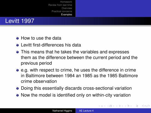
How to use the dataLevitt first-differences his dataThis means that he takes the variables and expressesthem as the difference between the current period and theprevious periode.g. with respect to crime, he uses the difference in crimein Baltimore between 1984 an 1985 as the 1985 Baltimorecrime observationDoing this essentially discards cross-sectional variationNow the model is identified only on within-city variation
Nathaniel Higgins AE Lecture 4

HomeworkReview from last time
OverviewPractical concerns
Examples
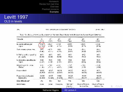
Levitt 1997Table 3
280 THE AMERICAN ECONOMIC REVIEW JUNE 1997
TABLE 3-ESTIMATES OF THE ELASTICITY OF VIOLENT CRIME RATES WITH RESPECT TO SWORN POLICE OFFICERS
Variable (1) (2) (3) (4) (5) (6) OLS OLS 2SLS 2SLS 2SLS LIML
In Sworn officers per 0.28 -0.27 -1.39 -0.90 -0.65 -1.16 capita (0.05) (0.06) (0.55) (0.40) (0.25) (0.38)
State unemployment rate -0.65 -0.25 -0.00 -0.19 -0.13 -0.02 (0.40) (0.31) (0.36) (0.33) (0.32) (0.33)
In Public welfare spending -0.03 -0.03 -0.03 -0.03 -0.02 -0.03 per capita (0.02) (0.02) (0.02) (0.02) (0.02) (0.02)
In Education spending per 0.04 0.06 0.02 0.03 0.05 0.03 capita (0.07) (0.06) (0.07) (0.07) (0.06) (0.06)
Percent ages 15-24 in 1.43 -2.61 -1.47 -2.55 -2.02 -1.50 SMSA (1.00) (3.71) (4.12) (3.88) (3.76) (3.86)
Percent black 0.010 -0.017 -0.034 -0.025 -0.022 -0.031 (0.003) (0.011) (0.015) (0.013) (0.012) (0.013)
Percent female-headed 0.003 0.007 0.040 0.023 0.018 0.033 households (0.006) (0.023) (0.030) (0.027) (0.025) (0.027)
Data differenced? No Yes Yes Yes Yes Yes
Instruments: None None Elections Election * Election * region Election * region city-size interactions interactions interactions
P-value of cross-crime <0.01 <0.01 0.09 0.13 0.33 0.28 restriction on police elasticity
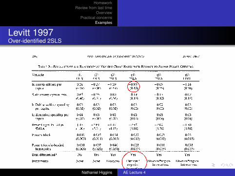
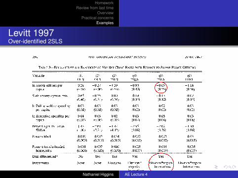
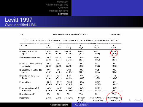
Notes: Dependent variable is Aln crime rate per capita for one of the four violent crimes (murder and nonnegligent manslaughter, rape, robbery, and aggravated assault), except in column (1) where log-levels, rather than log-differences, are used. Right-hand-side variables also are differenced in columns (2)-(6). Estimates are obtained estimating all crime categories jointly, allowing for a city-fixed effect across crime rates and heteroskedasticity across crime categories. The reported parameter estimates are constrained to be the same across all violent crime. Corresponding results for property crime are reported in Table 4. Number of observations is 1,136 per crime category. Crime-specific year dummies, region dummies, and city-size indicators also are included in all regressions. The reported coefficient for sworn officers is the sum of the contemporaneous and once-lagged coefficients. In columns (3)-(6), sworn officers are treated as endogenous. Column (3) instruments using mayoral and gubernatorial election-year indicators. Column (4) instruments using inter- actions between the city-size indicator variables and mayoral and gubernatorial elections. Columns (5) and (6) instruments using interactions between region dummies and mayoral and gubernatorial elections. The last row of the table reports the p-value of the restriction that the effect of sworn officers is identical across all four crime categories.
Table 3 shows the estimates for violent crime, imposing the cross-crime parameter restrictions described above. Column ( 1 ) presents OLS estimates of equation (3) in log-levels. The positive coefficient on sworn officers (0.28 with a standard error of 0.05) implies that more police are associated with higher crime rates. This result is consistent with previous estimates in the literature that rely on cross-city variation and do not take into account the endogeneity of the size of the police force (Cameron, 1988). Column (2) shows OLS results of equation (3) in log-differences. By first-differencing, all of
the parameters are identified using only within-city variation over time. The coef- ficient on sworn officers now becomes neg- ative (-0.27 with a standard error of 0.06), suggesting that unobserved heterogeneity across cities imparts an upward bias on the coefficient.
Columns (3) - (5) of Table 3 provide 2SLS estimates of the impact of police on crime us- ing a varying set of election-year interactions as instruments for sworn officers. The other variables continue to be assumed exogenous. In column (3), separate indicator variables for contemporaneous and once-lagged may-
Nathaniel Higgins AE Lecture 4
HomeworkReview from last time
OverviewPractical concerns
Examples
Levitt 1997OLS in levels
Nathaniel Higgins AE Lecture 4

HomeworkReview from last time
OverviewPractical concerns
Examples
Levitt 1997OLS in differences
Nathaniel Higgins AE Lecture 4

HomeworkReview from last time
OverviewPractical concerns
Examples
Levitt 1997Just-identified 2SLS
Nathaniel Higgins AE Lecture 4
HomeworkReview from last time
OverviewPractical concerns
Examples
Levitt 1997Over-identified 2SLS
Nathaniel Higgins AE Lecture 4
HomeworkReview from last time
OverviewPractical concerns
Examples
Levitt 1997Over-identified 2SLS
Nathaniel Higgins AE Lecture 4
HomeworkReview from last time
OverviewPractical concerns
Examples
Levitt 1997Over-identified LIML
Nathaniel Higgins AE Lecture 4
HomeworkReview from last time
OverviewPractical concerns
Examples
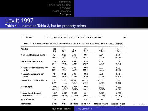
Levitt 1997Table 4 — same as Table 3, but for property crime
VOL 87 NO. 3 LEVITT: USING ELECTORAL CYCLES IN POLICE HIRING 281
TABLE 4-ESTIMATES OF THE ELASTICITY OF PROPERTY CRIME RATES WITH RESPECT TO SWORN POLICE OFFICERS
Variable (1) (2) (3) (4) (5) (6) OLS OLS 2SLS 2SLS 2SLS LIML
In Sworn officers per capita 0.21 -0.23 -0.38 -0.05 -0.24 -0.34 (0.05) (0.09) (0.83) (0.59) (0.36) (0.54)
State unemployment rate 1.40 0.99 1.04 0.94 1.01 1.04 (0.46) (0.46) (0.55) (0.50) (0.47) (0.49)
In Public welfare spending per 0.01 -0.02 -0.02 -0.02 -0.02 -0.02 capita (0.03) (0.03) (0.04) (0.04) (0.03) (0.03)
In Education spending per 0.51 0.01 0.01 0.02 0.01 0.01 capita (0.08) (0.09) (0.11) (0.10) (0.09) (0.10)
Percent ages 15-24 in SMSA 1.43 1.15 -1.47 -2.55 -2.02 2.69 (1.00) (4.92) (4.12) (3.88) (3.76) (5.16)
Percent black -0.002 -0.019 -0.029 -0.021 -0.022 -0.027 (0.003) (0.014) (0.018) (0.016) (0.015) (0.016)
Percent female-headed 0.007 0.013 0.025 0.012 0.016 0.022 households (0.006) (0.030) (0.039) (0.034) (0.031) (0.034)
Data differenced? No Yes Yes Yes Yes Yes
Instruments: None None Elections Election * Election * region Election * region city-size interactions interactions interactions
P-value of cross-crime <0.01 0.18 0.91 0.92 0.96 0.93 restriction on police elasticity
Notes: Dependent variable is Aln crime rate per capita for one of the three property crimes (burglary, larceny, or motor vehicle theft), except in column (1) where log-levels, rather than log-differences, are used. Right-hand-side variables also are differenced in columns (2)-(6). Estimates are obtained estimating all crime categories jointly, allowing for a city- fixed effect across crime rates and heteroskedasticity across crime categories. The reported parameter estimates are constrained to be the same across all property crime. Number of observations is 1,136 per crime category. Corresponding results for violent crime are reported in Table 3. Crime-specific year dummies, region dummies, and city-size indicators also are included in all regressions. The reported coefficient for sworn officers is the sum of the contemporaneous and once-lagged coefficients. In columns (3)-(6), sworn officers are treated as endogenous. Column (3) instruments using mayoral and gubernatorial election-year indicators. Column (4) instruments using interactions between the city-size indicator variables and mayoral and gubernatorial elections. Columns (5) and (6) instruments using interactions between region dummies and mayoral and gubernatorial elections. The last row of the table reports the p-value of the restriction that the effect of sworn officers is identical across all three crime categories.
oral and gubernatorial election years are used as instruments (since both contemporaineous and once-lagged police are included as re- gressors).18 The police coefficient, while imprecisely estimated, is nonetheless statisti- cally significant at the 0.05 level and is five times larger than the OLS estimates in column
(2).'9 Columns (4) and (5) expand the set of instruments by interacting the election-year dummies with four city-size indicators and nine census-region dummies, respectively. As the number of instruments increases in col- umns (4) and (5), both the coefficient esti- mates and the standard errors shrink. The estimates remain statistically significant,
8 Because the seven crime categories are stacked, each of the instruments is interacted with seven crime-category indicator variables in the actual estimation. A similar pro- cedure is used in columns (4) - (6).
'9 Estimates using only mayoral or only gubernatorial elections yield similar results, but are less precise.
Nathaniel Higgins AE Lecture 4
HomeworkReview from last time
OverviewPractical concerns
Examples
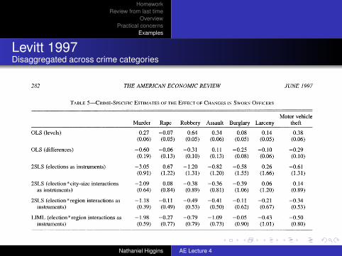
Levitt 1997Disaggregated across crime categories
282 THE AMERICAN ECONOMIC REVIEW JUNE 1997
TABLE 5-CRIME-SPECIFIC ESTIMATES OF THE EFFECT OF CHANGES IN SWORN OFFICERS
Motor vehicle Murder Rape Robbery Assault Burglary Larceny theft
OLS (levels) 0.27 -0.07 0.64 0.34 0.08 0.14 0.38 (0.06) (0.05) (0.05) (0.06) (0.05) (0.05) (0.06)
OLS (differences) -0.60 -0.06 -0.31 0.11 -0.25 -0.10 -0.29 (0.19) (0.13) (0.10) (0.13) (0.08) (0.06) (0.10)
2SLS (elections as instruments) -3.05 0.67 -1.20 -0.82 -0.58 0.26 -0.61 (0.91) (1.22) (1.31) (1.20) (1.55) (1.66) (1.31)
2SLS (election*city-size interactions -2.09 0.08 -0.38 -0.36 -0.39 0.06 0.14 as instruments) (0.64) (0.84) (0.89) (0.81) (1.06) (1.20) (0.89)
2SLS (election*region interactions as -1.18 -0.11 -0.49 -0.41 -0.11 -0.21 -0.34 instruments) (0.39) (0.49) (0.53) (0.50) (0.62) (0.67) (0.53)
LIML (election* region interactions as -1.98 -0.27 -0.79 -1.09 -0.05 -0.43 -0.50 instruments) (0.59) (0.77) (0.79) (0.73) (0.90) (1.01) (0.80)
Notes: Dependent variable is Aln crime rate per capita for the named crime category, except in row 1 where log-levels, rather than log-differences, are used. Right-hand-side variables also are differenced in columns 2-6. Each row of the table presents crime-specific coefficients on the sworn-officer variables from a separate regression. The reported coefficients, which are elas- ticities, represent the sum of the contemporaneous and once-lagged coefficients. In all cases, specifications are identical to that used in Tables 3 and 4, except that the cross-clime restrictions on police elasticities in Tables 3 and 4 have been removed in this table. All crime categories are estimated jointly, allowing for a city-fixed effect across crime rates and heteroskedasticity across crime categories. Controls for state unemployment rates, public welfare, and education spending per capita, percent of the population between the ages of 15 and 24, percent of blacks, and percent of female-headed households also are included in all regressions, as are crime-specific year dummies, region dummies, and city-size indicators. In row 3, sworn officers are treated as endogenous. Column 3 instruments using mayoral and gubernatorial election-year indicators. Row 4 instruments using interactions between the city-size indicator variables and mayoral and gubernatorial elections. Rows 5 and 6 instruments using interactions between region dummies and mayoral and gubernatorial elections.
however, and are two to three times larger than the OLS estimates.
Expanding the set of instruments may lead to more efficient estimation, but also in- creases the likelihood that 2SLS will per- form poorly. In the case of instruments that are only weakly correlated with the endog- enous regressor, it has been demonstrated that 2SLS is both likely to be biased towards OLS and to converge to asymptotic proper- ties at a slow rate (Paul A. Bekker, 1994; Douglas Staiger and James StQck, 1994; John Bound et al., 1995). The shrinking pattern of coefficients moving across col- umns (3) - (5) is consistent with poor finite- sample performance of 2SLS biasing the estimates towards the OLS estimates. As Joshua Angrist et al. (1995) demonstrate, however, limited information maximum- likelihood (LIML) estimation, while sensi- tive to other forms of misspecification, has favorable finite-sample properties in the presence of many weakly correlated instru-
ments. Column (6) of Table 3 presents the analog to column (5), estimated using LIML rather than 2SLS.2' The coefficient on sworn officers is now -1.16, almost as large as the 2SLS estimate with the smaller set of instru- ments, suggesting that the 2SLS estimates in columns (4) and (5) may be biased towards OLS. The standard error also increases vis- a-vis column (5), implying that the asymp- totic standard errors reported in column (5) are exaggeratedly low.
Table 4 presents estimates of equation (3) for property crime. As in Table 3, cross-crime parameter restrictions are imposed. The results for property crime display a somewhat differ- ent pattern of coefficients than was the case
20 Using LIML on the specification in column (3) yields almost identical police coefficients as 2SLS. The LIML estimates of column (4) appear exaggeratedly neg- ative, highlighting the sensitivity of LIML to the particular choice of specification.
Nathaniel Higgins AE Lecture 4
HomeworkReview from last time
OverviewPractical concerns
Examples
Levitt 1997Conclusions
Lots of the “offending” variation in the police/crimeinteraction seems to come from inter-city variation, whichis easily eliminated by first-differencingPattern of models (identified, overidentified, and LIML) isconsistent with the broad intuitionIV estimates are imprecise because of weak instrumentsIV estimates do suggest, however, that police reduce crime
Nathaniel Higgins AE Lecture 4