IOf

AD-A239 297

July 1991

Applications of Wavelets to RadarData Processing

• . ~~ ,,.3

Final Technical Report "'

1 CLIN 0002AA

1,,"

Principal Investigator Program Manager i fMr. Charles Stirman Dr. Arje Nachmann

U Sponsored byDefense Advanced Research Projects Agency

DARPA Order No. 7450Monitored by AFOSR Under Contract No. F49620-90-C-0050

I Martin Marietta Electronics,Information, and Missiles Group

P.O. Box 555837 .Orlando, Florida 32855-5837

I 91 2CF IP

S Form Approved

REPORT DOCUMENTATION PAGE OM ANpo70o0d8

Public reortifi burefl for thiS coIleCtioln of information is -st;-at t' I .o a erage i hour doer esporse. includin.g the time for revlewir g instructions. searching existng data sources.gatheerrq and 'ailtainmiglg the data needed. and comoleting and rev we-rq t.e ,:,31ecton of information Send comments reqardnqg this burden estimate or any mther asoect of thiscollection 0f M ormotOn. rcluding suggestions for reclucin, i-'s o'irden iashngton Headquarters Services. Directorate for information Ooerations and Reorts. 12 15 etersonDavisHi~ hnav. Suite 12C4. ilington. JA 22202-4302, and to to i )ff, )f Management and Budget. vaOerwori, Reouction Project (0704.0188). Washington. C 20503

1. AGENCY USE ONLY (Leave blank) 12. REPORT DATE |3. REPORT TYPE AND DATES COVEREDFINAL 27 Aug 90 to 26 Apr 91

4. TITLE AND SUBTITLE S. FUNDING NUMBERS

APPLICATIONS OF WAVELETS TO RADAR DATA PROCESSING F49620-90-C-0050

61101E 7450/006. AUTHOR(S)

MR. CHARLES STIRMAN7. PERFORMING ORGANIZATION NAME(S) AND ADDRESS(ES) 8. PERFORMING ORGANIZATION

REPORT NUMBERMARTIN MARIETTA CORPORATION MISSILE SYSTEMSP.O. BOX 555837 A-O"rn -ORLANDO, FL 32855-5837 1 ]. 1 *e s

9. SPONSORING / MONITORING AGENCY NAME(S) AND ADDRESS(ES) 10. SPONSORING/ MONITORINGAGENCY REPORT NUMBER

APOSR/=N F49620-90-C-0050eld 410

BollingA AJ DC U532-44d

11. SUPPLEMENTARY NOTES

Ila. DISTRIBUTION AVAILABILiTY STATEMENT 12b. DISTRIBUTION CODE

ApproVda fop Dbll releasedittrllbtloa Itlimltdo..

13. ABSTRACT (Maximum 200 words)

In this study, the recent mathematical theory of wavelets wasintroduced to the engineering problems of designing radar systems,radar processors, and radar algorithms. The goal was to make radarsmore efficient or more effective by the use of wavelets. Tounderstand why particular possible applications of wavelets to radarswere examined, it is necessary to understand some backgroundinformation on both radars and wavelets theory.

14. SUBJECT TERMS 15. NUMBER OF PAGES

16. PRICE CODE

17. SECURITY CLASSIFICATION 18. SECURITY CLASSIFICATION 19. SECURITY CLASSIFICATION 20. LIMITATION OF ABSTRACTOF REPORT OF THIS PAGE OF ABSTRACT

UNCLASSIFIED I UNCLASSIFIED I UNCLASSIFIED UlLSJSN 7940-01-280-5500 Sadr o,.r) e

!

U OA 11606IJuly 1991

Applications of Wavelets to Radar* Data Processing

I Final Technical Report

I CLIN 0002AA

I=

Principal Investigator Program ManagerMr. Charles Stirman Dr. Arje Nachman

ISponsored by

Defense Advanced Research Projects AgencyDARPA Order No. 7450

Monitored by AFOSR Under Contract No. F49620-90-C-0050

IMartin Marietta Electronics,

Information, and Missiles GroupP.O. Box 555837

Orlando, Florida 32855-5837

I

II

FINAL TECHNICAL REPORT

I CLIN 0002AA

APPLICATIONS OF WAVELETS TO RADAR DATA PROCESSING

5 ARPA Order 7450

Program Code 0D20

I Name of Contractor - Martin Marietta CorporationMissile Systems

Effective Date of Contract - August 27, 1990

Contract Expiration Date - July 26, 1991

I Amount of Contract Dollars - $192,806

Contract Number - F49620-90-C-0050

Principal Investigator - Mr. Charles Stirman407-356-2573

I Program Manager - Dr. Arje Nachman202-767-5025

Title of Work - Applications of Wavelets to Radar DataProcessing

ISponsored by

Defense Advanced Research Projects AgencyDARPA Order No. 7450

Monitored by AFOSR Under Contract No. F49620-90-C-0050

The views and conclusions contained in this documentare those of the authors and should not be interpretedas necessarily representing the official policies orendorsements, either expressed or implied, of theDefense Advanced Research Projects Agency or the U.S.government.

II

TABLE OF CONTENTSI1 SUMMARY 1

1.0 Final Report Summary 1

2 WAVELETS METHODS 62.0 Compactly Supported Wavelets 62.1 The Scaling Function, Wavelets, and the 9

Wavelet Transform2.2 The Scaling Function 102.3 Wavelets 132.4 The Wavelet Transform 152.5 The Computational Complexity of Wavelet 17

Transforms

3 RADAR METHODS AND MAIN RESULTS 203.0 Basic Radar System Operation 203.1 The Millimeter Radar Data Base 213.2 Wavelet Approximation to the FFT 293.3 Target Length Estimation 343.4 Wavelet Target Classification Results 393.5 Fine Range Resolution by Wavelets 41

4 ADDITIONAL RESULTS 434.0 Supplemental Results 43

APPENDICES 72A. List of Symbols 72B. Wavelet Transform Theory 73

B.1 Wavelets and Wavelet Transforms 73B.2 Wavelet Approximation to the Fourier 77

TransformB.3 Computational Complexity of the Wavelet 82

Approximation to the Fourier TransformC. Phase Unwrapping 88D. Martin Marietta Radar Data and Pulse 95

Compression ProcessingD.1 Time-Frequency Pulse Compression 96D.2 Characteristics of the Millimeter Wave 99

Radar Data used in this Study

E. Baseline Target Extent Calculation Method 106

BIBLIOGRAPHY 107

I ii

FIGURES

I2.1 Scaling Functions2.2 Wavelets2.3 Wavelet Transform2.4 Sub-band Tree Structure2.5-2.6 Wavelet Transform Computational Complexity3.1 Radar Block Diagram3.2 Wavelet Impact Areas3.3-3.6 Wavelet Reconstruction of Target Profiles3.7-3.11 Wavelet FFT Approximation Results3.12-3.15 Target Length Estimation Results3.16 Wavelet Classifier Results3.17 Wavelet Waveforms for Radars4.1-4.3 Wavelet Reconstruction of a Trihedral4.4-4.6 Wavelet Reconstruction of two Dihedrals4.7-4.18 Truck Even Polarization Length Estimation Results4.19-4.30 Truck Odd Polarization Length Estimation Results4.31-4.42 Tank Even Polarization Length Estimation Results4.43-4.54 Tank Odd Polarization Length Estimation ResultsB.1-B.3 Wavelet FFT Approximation ComputationsC.1-C.8 Phase Unwrapping ComparisonsD.1-D.9 Radar Data Plots

III

Ii

1.0 Final Report Summary

3 Technical Problem

The technical problem addressed by this contract was todetermine the feasibility of exploiting the emerging mathe-matical theory of wavelets in radar system applications.The work to be done was divided into three tasks.1. Perform a preliminary systems benefit study. Address

the complete radar processing problem including theapplicability of wavelets to the various processingelements: prescreener, fast Fourier transform (FFT),IR classifier, and automatic target recognizer (ATR).

2. Define and develop appropriate wavelet methods for radarapplications.

3. Determine the stability of the wavelet transform image.Make a comparison of wavelet transforms and FFT signaturesfor each of three targets: a set of calibrated cornerreflectors of known radar cross section and spacing, anI M60 tank, and an M35 truck.

Three specific potential applications of wavelets methods toradar systems were identified for investigation.1. Use wavelets to transform the data that forms the input to

the radar's ATR algorithms.2. Modify a typical radar system so that if a wavelet

transform (which is faster than an FFT) replaces the FFT(which is currently used), the output is still a highrange resolution target profile.

3. Develop a wavelet approximation to an FFT such that thewavelet approximation is sufficiently accurate and fasterthan an FFT.

Methodology

In this study, the recent mathematical theory ofwavelets was introduced to the engineering problems ofdesigning radar systems, radar processors, and radaralgorithms. The goal was to make radars more efficient ormore effective by the use of wavelets. To understand whyparticular possible applications of wavelets to radars wereexamined, it is necessary to understand some backgroundinformation on both radars and wavelets theory. These topicsare discussed briefly in the following paragraphs. Also,Ithe Martin Marietta radar data that was used in this studyis described, and some description is given of typicalprocessing methods for this data.

Modern radar systems transmit and receive frequency-stepped radio frequency (RF) waveforms. The radar signalprocessor transforms the received data by using an FFT.Since the FFT forms a matched filter with the frequency-stepped waveforms, the vector whose components are themagnitudes of the complex data output from the FFT forms ahigh range resolution profile (HRRP) of the objects in theradar beam. These HRRPs are the inputs to the radar's ATR

II

processor. Both FFT and ATR calculations are computationintensive and impose difficult and costly requirements on theradar signal processor. Wavelet methods were examined forpotential efficiency improvements in FFT or ATR processors aswell as for potential ATR performance improvements.

Investigations utilized Martin Marietta's short pulse,frequency-stepped, fully calibrated 35 Ghz radar data. Thisdata utilized two transmit (right hand circular and left handcircular) and two receive (right hand circular and left handcircular) radar polarizations (right and left circular) andresulted in a complete polarization set of four receive-transmit pairs. Transmitting right or left and receiving theopposite yields "odd" polarized returns. If the receiver hasthe same polarization sense as the transmitter, the return is

an "even" polarization. The data is coherent which allowscreation of HRRPs. Figures 3.3 through 3.6 show odd and evenHRRPs. There are radar looks at an M60 tank and an M35 truckat every hundredth of a degree of aspect in this data set. Aradar look consists of 64 coherent, frequency stepped timesamples for the four receive-transmit polarization pairs.Each polarization of each radar look can be processed throughan FFT to produce an HRRP of the vehicle in the radar's view.Compactly supported wavelets are a family of recentlydiscovered (1986) mathematical functions that have beensuccessfully applied to problems in image compression, audiocompression, vision analysis, and transient signal analysis.The wavelet methods used on this contract employed compactlysupported wavelets that generated orthonormal bases. Par-ticular wavelets used were denoted D2, D4, D6, and D8 inhonor of Ingrid Daubechies, who developed the theory oforthonormal bases of compactly supported wavelets. The D2wavelet is also known as the Haar wavelet. A wavelet basisconsists of a "scaling function" 0(x) that is the solution toa recursion equation derived from orthogonal subspaceprojection mathematics, a basic wavelet function woo(x) thatis derived from the scaling function, and a countablyinfinite collection of wavelet functions Wjk(X) that aredilations (frequency changes) and translations (time shifts)of the basic wavelet function. The recursion equation is

Igiven by 0(x) = 1CkO(2x-k)and the wavelet functions are defined by

Woo (X) = J(-1)kc -ko(2x-k)W jk(X) = 2J/ 2 woo(2ix-k).

Some specific linear operations involving the recursioncoefficients Ck can compute wavelet coefficients and waveletapproximations to functions very rapidly since only a few ofthe Ck are nonzero.

Not all wavelets have compact support nor do they allgenerate orthogonal bases. However, throughout this reportthe terms wavelets and compactly supported wavelets are usedinterchangeably, and wavelet bases are assumed to be orthog-

onal. Results presented were produced using specificcompactly supported wavelets.

!2

II

Technical Results

Results clearly demonstrate that, under certain circum-stances, wavelets methods can improve radar system perform-ance. These wavelet results and their radar system appli-cations are summarized below and described in detail inSections 3.2, 3.3, 3.4, and 3.5 of this report.

The radars considered in this study were millimeter wave(MMW) radars, but results obtained are also applicable toradars of other wave lengths. MMW radars are typicallyeither pulse radars with short radar pulse lengths orfrequency modulated continuous waveform (FMCW) with longradar pulse lengths. There is a major difference betweenthese two types of MMW radars as far as wavelets applicationsare concerned. This is due to the fact that if one wants agiven range resolution in the HRRP, one must compute an FFTof very large dimension for an FMCW radar but a relativelysmall FFT for a pulse radar.

The most significant application of wavelet methods toradars involves the radar's ATR algorithms' capability andcomplexity. The data base of full polarization, calibrated,coherent MMW radar returns from tanks and trucks was used forthis study. This data base also contained radar looks at thecalibration reflectors consisting of a single trihedral anda pair of dihedrals of known radar cross section. The majorgoal was to reduce the dimension of the HRRP radar datavector without losing information that is important to theATR. There are three distinct reasons why this dimensionreduction could improve the ATR.1. The reduced dimension that serves as the input to the ATR

may allow use of a more complex and effective (higherorder polynomial classifier, for example) classifier ortarget-clutter discriminator algorithm within thecomputational limitations of the ATR digital signalprocessor.

2. Reduced dimension may make the choice of the type of ATRclassifier and/or target-clutter discriminator obvious;consequently, ATR performance could be improved.

3. Even if reduced dimension does not suggest a change inthe type of classifier or discriminator algorithm, it maygreatly reduce the number of computations requiredby the ATR thereby increasing the speed and decreasing thehardware requirements of the ATR.

As a test case for the ability of wavelets to reduceHRRP dimension, one feature - "target length" - was examined.For this effort, Martin Marietta defined the problem andmonitored the results while our subcontractor, Aware, Inc.,provided the wavelets expertise and produced the results.Wavelet algorithms and typical target length estimationtechniques were applied to the radar HRRP data base. Results

showed that when appropriate wavelet methods were applied

I3

II

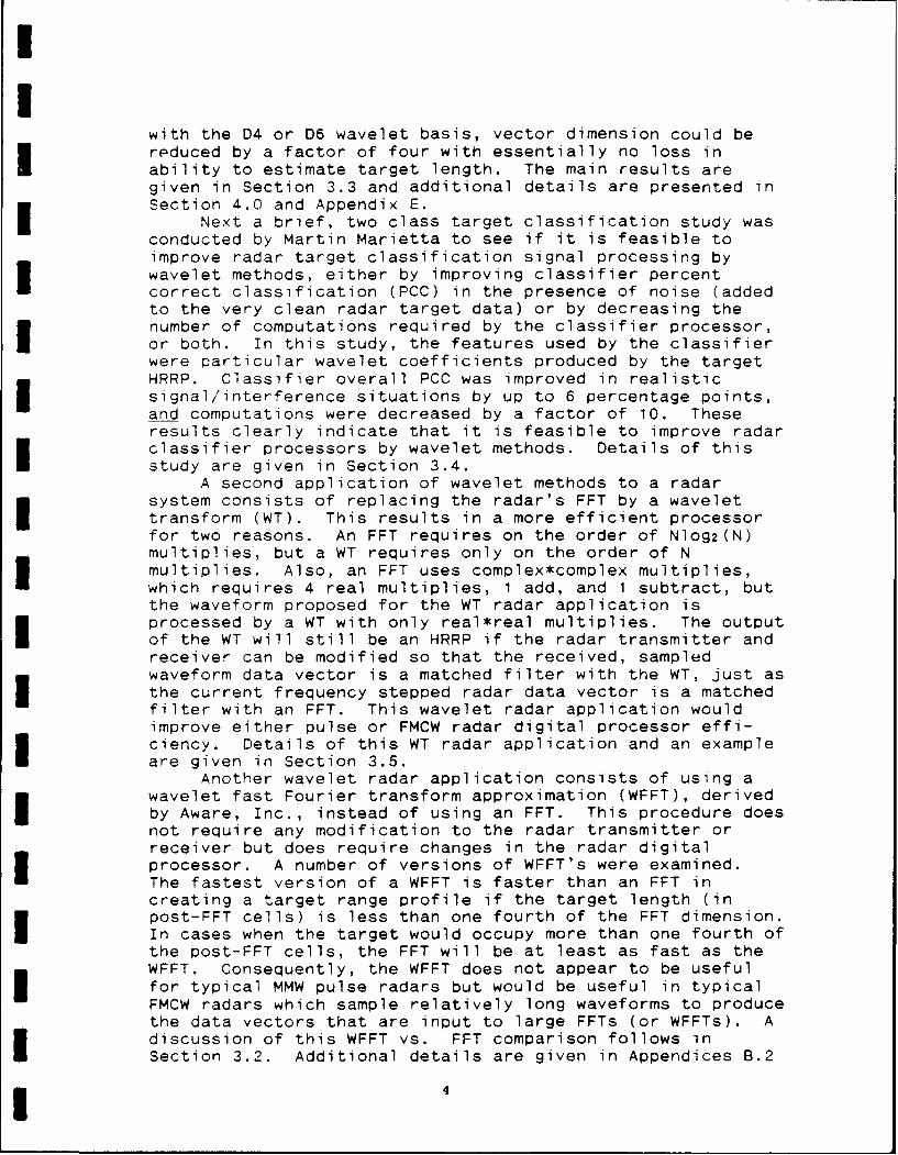
with the D4 or D6 wavelet basis, vector dimension could bereduced by a factor of four with essentially no loss inability to estimate target length. The main results aregiven in Section 3.3 and additional details are presented inSection 4.0 and Appendix E.

Next a brief, two class target classification study wasconducted by Martin Marietta to see if it is feasible toimprove radar target classification signal processing bywavelet methods, either by improving classifier percentcorrect classification (PCC) in the presence of noise (addedto the very clean radar target data) or by decreasing thenumber of computations required by the classifier processor,or both. In this study, the features used by the classifierwere particular wavelet coefficients produced by the targetHRRP. Classifier overall PCC was improved in realisticsignal/interference situations by up to 6 percentage points,and computations were decreased by a factor of 10. Theseresults clearly indicate that it is feasible to improve radarclassifier processors by wavelet methods. Details of thisstudy are given in Section 3.4.

A second application of wavelet methods to a radarsystem consists of replacing the radar's FFT by a wavelettransform (WT). This results in a more efficient processorfor two reasons. An FFT requires on the order of Nlog2(N)multiplies, but a WT requires only on the order of Nmultiplies. Also, an FFT uses complex*complex multiplies,which requires 4 real multiplies, 1 add, and 1 subtract, butthe waveform proposed for the WT radar application isprocessed by a WT with only real*real multiplies. The outputof the WT will still be an HRRP if the radar transmitter andreceiver can be modified so that the received, sampledwaveform data vector is a matched filter with the WT, just asthe current frequency stepped radar data vector is a matchedfilter with an FFT. This wavelet radar application wouldimprove either pulse or FMCW radar digital processor effi-ciency. Details of this WT radar application and an exampleare given in Section 3.5.

Another wavelet radar application consists of using awavelet fast Fourier transform approximation (WFFT), derivedby Aware, Inc., instead of using an FFT. This procedure doesnot require any modification to the radar transmitter orreceiver but does require changes in the radar digitalprocessor. A number of versions of WFFT's were examined.The fastest version of a WFFT is faster than an FFT increating a target range profile if the target length (inpost-FFT cells) is less than one fourth of the FFT dimension.In cases when the target would occupy more than one fourth ofthe post-FFT cells, the FFT will be at least as fast as theWFFT. Consequently, the WFFT does not appear to be usefulfor typical MMW pulse radars but would be useful in typicalFMCW radars which sample relatively long waveforms to producethe data vectors that are input to large FFTs (or WFFTs). Adiscussion of this WFFT vs. FFT comparison follows inSection 3.2. Additional details are given in Appendices B.2

I4

I1

and B.3.

* Further Research

This wavelets radar applications feasibility study haspointed out several areas for further useful research.

Wavelet dimension reduction capabilities may improveother radar ATR algorithms, either by improving stabilityversus signal-to-interference and/or by decreasing compu-tational complexity. Also, wavelets methods may prove evenmore useful in two-dimensional ATR applications such assynthetic array radar, infrared imaging, or electro-opticalimaging.

If there is an FMCW system whose targets are small inlength relative to the radar pulse length, this stuayindicates that it would be appropriate for that system tofurther investigate implementing WFFTs rather than FFTs.

Several questions remain concerning the possible use ofWTs to replace FFTs in a radar. What wavelet basis producesthe radar waveform that is most appropriate for transmissionand reception by a radar system such that the WT would outputHRRPs? Can such a system be built? Is the increased effi-ciency of the WT (over the FFT) sufficient to offset the costof the changes required in the transmitter and receiver?

UAcknowledgementWe are indebted to Howard Resnikoff and Charles Smith

along with their staff at Aware, Inc. for their time andeffort expended in support of this contract. It was theirexpertise in wavelet technology and their willingness toentertain a myriad of fundamental questions which permittedMartin Marietta to formulate and successfully complete ameaningful feasibility study in applicability of waveletmethods to radar systems.

Several sections (2.0 through 2.5, 3.2, 3.3, 4.0, andthe Appendices) are based on input received from Aware, Inc.However, conclusions and results as they relate to the ATR

*classifier are solely those of Martin Marietta.

I5

I

2.0 Compactly Supported Wavelets

A major reason for conducting this study is the remarkableresults being obtained through the application of compactlysupported (zero outside a finite interval) wavelets to signalprocessing. Compactly supported wavelets are a class ofmathematical functions that were discovered in 1986. Some of theparticular advantages of wavelet signal processing methods are:

o Wavelet transforms are computationally efficient. Thenumber of arithmetic operations required to perform awavelet transform is linearly proportional to the number ofinput data points. The computational complexity of theI more traditional Fast Fourier Transform (FFT) isproportional to the number of input data points times thelogarithm (base 2) of the number of input data points. Forlarge problems, the wavelet methods require only a fraction

-- of the number of operations required by the traditionalmethods. This advantage increases as the problem sizeincreases. In addition, wavelet transform algorithms canIbe directly implemented in very large scale integration(VLSI) logic devices, and they are fully parallelizable.

o Wavelet transform methods can analyze signals in both thetime and frequency domains. The relative resolution of thetime and frequency components can be flexibly adapted tothe problem at hand. The selection of the appropriateI] time-frequency resolution can be done upfront at systemdesign time or it can be accomplished with real-timeadaptive algorithms. The traditional Fourier transformsuffers from very poor (or nonexistent) time resolution.This particularly limits its usefulness in the analysis oftime-limited (i.e., transient) signals. There have beenattempts to modify the Fourier technique in various ways toovercome this limitation, but all of the methods introducesome additional complexities and compromises. Waveletmethods offer a very natural means to performtime-frequency signal analysis.

o Wavelets provide the flexibility to choose a particularwavelet function that is "customized" to the specificapplication. This is possible since compactly supportedwavelets are an infinite family of complete orthogonalbasis functions. This flexibility to choose basis

I functions can not be matched with the Fourier transform forit uses only a single set of basis functions - the complexexponentials (i.e., the sine and cosine functions.)

Compactly supported wavelets are a complete and orthogonalset of basis functions for the set of all finite energy discretesignals. The wavelet transform is invertible, energy-preservingand linear. The wavelet transform is a processing method whichanalyzes both continuous streams of input data and blocks of data.A multiplier 2 wavelet basis consists of a scaling function, a

6

I

basic wavelet and a collection of smaller wavelets. The smallerwavelets are created by "shrinking" the basic wavelet by a factorsof 2 and shifting (or translating) them by scaled integerdistances. Thus the collection of smaller wavelets are 1/2 and1/4 and 1/8 (and so on) the size of the basic wavelet. Whenever

the "wavelet length" shrinks by a factor of two, the "waveletfrequency" can be thought of as doubling. This shrinkage factoris sometimes called scale or scale level. Wavelet basis functionsare all related by multiples of the constant ratio (2 : 1). Thebasic wavelet is computed from the scaling function. Theselection of the scaling function determines all of the remainingbasis functions. A remarkable fact is that there are an infinitenumber of scaling functions, each of which defines a completewavelet basis. This provides tremendous flexibility in selectingbasis functions which are appropriate for different systems.

In general, the computational complexity of wavelet methodsis O(n), which means that the computational complexity is of ordern. The efficiency is the direct result of the simplicity of thewavelet transform process. The process starts by separating thesignal information in the smallest wavelets from information inall the larger wavelets scales. Details are given in Section 2.4.The output of the first stage is processed again by the samemethod and is repeated for each successive scale. This recursivestructure reduces the amount of data to be processed at eachsuccessive level by a factor of two which reduces thecomputational cost for each successive transform level.Information which varies rapidly over just a few data points isseparated from information which varies over many points. Theprocedure is stopped at the largest wavelet of interest.

The outputs of the wavelet transform are coefficients whichrepresent the similarity of the signal (as a function of time) tothe wavelets of different shrinkage factors and times. The outputof a wavelet transform can be plotted on a grid that has time onthe x-axis (or t-axis) and shrinkage factor on the y-axis. Thisgrid is called phase space and is used to graphically display therelationships between signal information at different shrinkagefactors and times.

It is helpful to compare and contrast the wavelet transformwith the well known Fourier transform. The Fourier transform isalso invertible, energy-preserving and linear. The Fourier basisfunctions are orthogonal and complete for the entire set of finiteenergy discrete signals.

The Fourier transform separates signal information byfrequency. The Fourier transform requires an a priori choice ofinput data block size. The Fourier basis functions are constantfrequency complex exponential functions each of which persists aslong as the block size. The basis functions are uniformly spacedin frequency. The frequencies are separated by a constantinterval rather than a constant ratio. Since all of the basisfunctions are as long as the input data block, they all have thesame (lack of) time resolution. The output of a Fourier transformcontains information about how the energy in the signal isdistributed among the frequencies in the signal. Howeverinformation about how the energy is distributed in time, about

I

Iwhen it occurred, is not available in the Fourier transformrepresentation. All that can be inferred is that the frequencywas present somewhere in the block and what fraction of the signalenergy it accounted. The computational complexity of the fastFourier transform (for the commonly used Cooley-Tukey algorithm)is O(nlog 2 (n)).

The Fourier transform separates signal information intouniformly spaced frequency components. The Fourier transform hasfine frequency resolution and a complete lack of time resolution.Increasing the input data block size increases the range offrequencies which the Fourier method can resolve, but decreasesthe time information available from a signal.

In summary, the primary difference between the Fouriertransform and the wavelet transform is in how each separatessignal information between time and frequency or a frequencyrelated parameter, shrinkage factor. Wavelet transforms separatesignal information by shrinkage factor and time. The number ofshrinkage factors used and the number of times resolved arejointly limited by the input data block size. There are aninfinite number of wavelet basis from which an appropriate basiscan be selected. The computational complexity of the wavelettransform is O(n), less than the Fourier transform 0(nlog 2 (n)).

IIIIIIII

I 2.1 The Scaling Function, Wavelets, and the WaveletTransform

Wavelet methods separate the components of a signal by timeand a shrinkage factor that is related to frequency. With awavelet transform, both the time resolution, or "correlationlength", and the shrinkage factor resolution vary logarithmically.

The wavelet technique takes into account the reciprocalrelationship between time and frequency (or any type of structurewhich is expressed across multiple data points). To identify orlocate the position of a particular shape, such as an oscillation,in a set of data, one must look for relationships among the datavalues; a structure or an oscillation exists only across a set ofdata, and not in a single point value. A number has no frequency,no structure. Conversely, properties which exist throughout a setof data cannot be said to have a particular location within thatset. Wavelet signal representation techniques take this trade-offinto account by allowing small sets of data to be combined andcorrelated to derive structural or shape information about thatsubset, without requiring a complete transformation of the signalinto a particular type of structural information, the way aFourier transform does. Thus, unlike the Fourier transform one isallowed to exchange a small amount of temporal resolution for asmall amount of information.

It is no accident that these properties are reflected in thecharacteristics of many natural signals. Signals with timevarying characteristics, like speech, music, seismic signals andunderwater acoustic signals are all best analyzed by a systemcapable of resolving both frequency and time. Furthermore, manysignal-producing phenomena have octave band structure due to thepresence of harmonics within the signal and respond well towavelet analysis. Transient events also respond well to waveletanalysis in that the identification of precisely locatedphenomena, such as the sharp onset of a signal, requires theability to resolve its location in time with a very shortwavelength, while the characteristics of later, more persistent,parts of the signal may require the ability to identify longerwave shapes.

Scaling functions, wavelets, and the wavelet transform arediscussed in more detail in the next three sections and also inAppendix B.

I 9

I

1 2.2 The Scaling Function

The scaling function is at the core of any wavelet basedrepresentation of a signal. We will discuss only compactlysupported wavelets in this report. The scaling function has threeessential properties. The first is that it is compactlysupported. This means that the scaling function is exactly zerooutside a bounded region of the real line. The scaling functionis only locally non zero.

The second essential property is that the scaling function isorthogonal to integer translates of itself. The importance ofthis will become clear a little later. The third property is thatthe scaling function is intimately related to smaller, or scaledversions of itself. This relationship is expressed concisely bythe scaling equation:

4 W(x) = ak q( 2 x - k) (2.1)

where 9(x) is the scaling function. The function v(2x) is acmaller, scaled down (by a factor of two), version of p(x). Thescaling equation states that 9(x) is equal to a weighted sum ofthese small versions of itself. The numbers ak, of which onlyfinitely many (N, which is an even number here) are non zero, arecalled the scaling coefficients. N is the size of the waveletsystem. The support of 9, the region on which it is non zero, isthe interval [0, N-1]. The coefficients Qk must satisfy certainconditions in order for the scaling function to exist and satisfythe scaling equation. There turns out to be an infinite number ofsets of scaling coefficients for every even N > 2. It is thechoice of the ak, from among this set, which determines thedetailed shape of 9(x).

Scaling functions are commonly selected from the class ofDaubechies functions, which have several importantcharacteristics. They are relatively smooth and have certainapproximation properties (i.e., vanishing moments). These systemswill be referred to as D2 (which is also the "Haar") D4, D6,D8... Dn, where n is the size of the system. The first fourDaubechies scaling functions are shown in Figure 2.1.

The scaling function is the basic unit from which a level ofIadetail is constructed. This is done by considering the set offunctions which can be represented as a linear combination ofshifted versions of the scaling function. That is, we define acollection of functions at "scale level" j, which we write Vj to bethe set of functions which are linear combinations of thefunctions 9(2Jx - k), where k is an integer. The factor 2Jmultiplying x has the effect of shrinking the support of 9 to theinterval from 0 to (N - 1)/2J, and the shift by k moves these smallfunctions around. Thus a function's components at scale level j

* are expressed by the equation:

10

I

fj(x) = cj,kP(2Jx - k) (2.2)kEz

where fj is the part of f resolvable at the scale level j.This idea can also be expressed by stating that Vj is the

space spanned by the set

{P(2Jx - k) IkEZ} . (2.3)

This set of functions forms an orthonormal basis for Vj. Functionsin Vj are uniquely expressible as linear combinations of the basisfunctions, and the basis functions all have unit "energy". Thusthe set of functions {1(2Jx - k) } form an orthogonal set of"templates" for Vj.

The effect of performing a transform with such a set of basisfunctions is to identify, within the signal, those parts orcomponents which are similar to the basis functions at the givenscale level. Similarly, a Fourier transform has oscillatoryfunctions as a basis, and identifies the relative contribution ofeach frequency to the overall signal.

With shifted versions of the scaling function as a basis, thewavelet transform will identify components which are similar to aparticular shifted copy of the scaling function; that is,representations of a function in the scaling function basisidentifies features locally in time, since the scaling function iscompactly supported, and locally in scale level, because thescaling function has structure.

There is another, equally good, set of orthogonal "templates"for this scale level Vj. This set of "templates" gives a differenttype of information than the one presented above. In our previousbasis, all of the resolution within the scale level j was in thetemporal domain: each coordinate corresponded to a position intime. The new basis will trade some of this temporal resolutionfor some additional structural information; for each scale levelit will give us two sets of coefficients, one set which represents

large structure, while the other set represents small ("fine")structure. The process extracts or filters out the components ofthe scale level j which cannot be regarded as part of the coarserscale level, j - 1.

IIII

0* 0.5-

1. 1

0 0.5

1 0*05 -0.5

0 0.5 0 1 2 3

111 11

I0- 0

0 0.5 0 2 2 3.8

2 1

0 0

-0.

-21 -2I0 0.5 0 12 43

Fiur 2.. ForEape1.Wvees(lcws5rm pe et Ha"

* 1

I

I 2.3 Wavelets

This idea of dividing the scale level Vj into a coarser version ofitself, Vj-,, and a difference space, which we will call Wj-i. canbe compactly expressed as an orthogonal splitting of the space Vjinto two perpendicular spaces Vj-i and WJ-1:

Vj = Vj_1 G Wj_ 1 . (2.4)

The reason this can be done efficiently comes from the scalingequation. Since 9(x) can be expressed as a linear combination oftranslated versions of V(2x) the coarser scale level Vj_. iscontained within the finer scale level Vj:

Vj-1 C Vj (2.5)

* Repetition of the argument shows that

Vj_1 C Vj C Vj+ 1 C Vj+2 . . . (2.6)

3 The difference space, WJ-l, contains all that remains when thecoarser scale information is removed. However, since Wj-j iscontained in Vj, it is also expressible as a linear combination oftranslates of T(2Jx).

The actual set of functions that are used to span the spaceWe-1 are the orthonormal basis formed by the functions3 N-i

W(2Jx) = N- (-1)kaN-kiP(2j+i x - k) (2.7)

or in the case of j =0,

N-1

I (1)kaNk-1l( 2 x - k) (2.8)k=O

3 Notice that the signs now alternate in the sum, and the order ofthe coefficients ak has been reversed (k - N - k - 1) . Thesechanges make W(x) orthogonal to p (x). The full basis for Wj isformed by taking shifted versions of a, i.e., Basis (Wj) =

{2J/2W(2Jx-k) Ik an integer}. The support of w(x) is easily seen tobe the same as the support of 9(x), and this is true for theshrunken versions as well, that is, the support of w(2Jx-k) is thesame as the support of WV(2x-k). The normalization term 2J/2maintains unit energy in the functions. Figure 2.2 shows thewavelets which correspond to the scaling functions presented inFigure 2.1.

Thus the transformation from the first representation of Vj,where fj was expressed as a linear combination of shifted versionsof iP(2Jx), to the new representation, where fj is expressed as aI sum of translates of 4p(2J-lx) and translates of W(2j-lx), gives usnew information about the shapes and structures, perhapsfrequencies, present in fj. This is at the expense of some temporal

13

U

I resolution, because the new basis functions are twice as long. Thenew basis incorporates the inter-relationships among largersubsets of the data, providing correlative information. As aresult of the spectral refinement, there has been a loss oftemporal resolution.

The scaling function, being the origin for all of the spacesVj, forms the connection between these spaces via the scalingequation, equation 2.1. The basic wavelet,W, represents thedifferences between the scale levels.

iIIiiIIIIIiiii

I 14

12.4 The Wavelet Transform

The exchange of temporal resolution in Vj for scale resolution inthe division of Vj into Vj- 1 and Wj-j forms the basic unit of theWavelet transform. Since the definition is independent of scalelevel, it can be repeatedly applied in the same way. Furthermore,Ithe operations involved in the transformation require only theexpansion coefficients of the function f(x) in the basis at thecurrent scale, and not the actual values of the function. Thecomputation is very simple and efficient because of the close linkbetween the functions 9 and W.

The basic operation involved in a wavelet transform is theconversion of temporal resolution into structural or spectralinformation. This basic single step, essentially a filter,exchanges half the temporal resolution of a signal for twice the"frequency" resolution; the product of the two remains the same.More importantly, this operation can be repeated to gain anydesired level of detail in the structural or spectral realm, whileonly imposing a reciprocal loss of resolution in the temporaldomain. This is in sharp contrast to Fourier transformtechniques, where one either gets all the available frequencyinformation, or none of it, with no intermediate stages ofknowledge available.

The wavelet transform allows one to move gradually betweenthe two extremes present in the Fourier transform, successivelygaining shape or structure information. In a sense, the wavelettransform interpolates between the frequency, or structure, domainand the temporal domain. This step by step transformation can beunderstood in terms of trade-offs between relative time resolutionand relative frequency resolution.

Since the transform is defined in terms of operations on thecoefficients of the representation, and not the actual values ofthe scaling or wavelet functions, the output from a single stageof the transform is exactly what the next stage requires forinput. This easily pipelined, recursive structure is what makesthe wavelet transform rapidly computable. While many suchstructures are made possible by the wavelet transform, one in

-- particular, the one-sided or Mallat transform, has proven to beexceptionally useful in analyzing signals. Figure 2.3 shows oneoperation of the wavelet transform. The second operation uses theI"low pass" (see Figure 2.4) output coefficients from the firststage as the input for the second stage, etc. The number of datapoints at each level is reduced by a factor of two by the3m conversion of temporal information into spectral information.

* 15

I "Low Pass"or

U (P Terms

3 Input

3 "Hifgh Pass"or

3 ~I Terms

Figure 2.3: One OPerati0fl of the Wavelet Transform

Fiue24IreSrcuefrte ata u-adTe nlss

I1

I

U 2.5 The Computational Complexity of Wavelet Transforms

This section is concerned with the computational efficiency ofwavelet-based analysis techniques. The computational complexityof several types of wavelet transforms is developed andcomparisons are made to the computational complexity of the FFT.Both pre- and post-processing requirements are ignorci. It isassumed that the output from the wavelet transform or FFT is thedesired result. The input block size is the factor whichdetermines the computational cost. The first case is a wavelettransform which resolves only a portion R=1/2 J of the totalbandwidth, and resolves it as finely as possible using recursivewavelet techniques. The simplest example of such a transform isthe familar Mallat Transform, which calculates the decompositionof a signal on the basis of scale, i.e., it "homes in" on lowfrequencies. This fundamental structure requires

OPS(Mallat) = a(K)N(I-l/2J) # of operations (2.9)

where a(K)=(K+I) multiplies and (K) additions per output point. Thenumber of input data is N, and J is the finest level calculated;that is, the basic wavelet decomposition operation is applied Jtimes. The number of nonzero coefficients is K, which we havealso called the length of the wavelet coefficient matrix. Notethat whatever the depth of the decomposition, the operation countnever exceeds a(K)N. This operation count also applies to anywavelet transform which "zooms in" on a single location in phasespace, allowing other side-bands to remain unchanged. These arenot partial wavelet transforms: each is a complete representationin a wavelet basis. Each is, however, a partial frequencydecomposition. That is a powerful advantage because only what isrequired need be calculated.

In applications where one wishes to resolve frequencies (orsome other structure) to some pre-specified resolution (say 1/2j),and one is interested in a small number of sub-bands, wavelets arevery computationally. efficient. This case includes the MallatTransform, and any other wavelet processing scheme which generatesIonly a small subset of the finest resolution cells.

If the application requires that the temporal resolutionexisting in a subband be converted to frequency or structureI information, the wavelet transform can be further applied in auniform fashion to derive this information, as in Figure 2.4.Since the formula for this case, equation 2.10, is rathercomplicated, comparisons were made with the complexity of an FFTcalculation for the full bandwidth of the signal, and forconsistency the wavelet transform was also carried to its fullresolution within the resolved subband. Since there areessentially no savings possible with an FFT for resolving only aportion of all subbands, the full complexity of 3n+nlog 2n was usedfor comparison.

17

I

I If we define

1. N = the number of data points;

2. K = the size of the wavelet filter (assumed to beconstant throughout the procedure) and a(K) is thecomputational cost for the fixed filter length;

3. R = the portion of the bandwidth of the signal which isresolved (assumed to be 1/2L for some L);

4. J = the finest level of resolution (the width of theI frequency bands resolved is 1/2J),

then the number of operations required to generate the desiredresults, along with all of the remai.,ing results that are requiredto have a complete representation, is:

a(K)N(1+R(J-2+Iog 2 (R))/2) (2.10)

I The comparison is summarized by Figures 2.5 and 2.6, (a(K) countsthe number of real multiplies) which show the filter length forwhich the two techniques are equally complex for a variety ofvalues of R. See Figure 2.4 for an example of such adecomposition.

Figures 2.5 and 2.6 relate increased wavelet computationalsdue to increased number of coefficients, K, to wavelet superiorityversus FFT (in terms of computations required), which increases asthe data block size increases.

iIIIIIII

I _ _ _ _ _ _ _ _ _ _ _ _ _ _ _ _ _ _ __14_ _

* 0.05

12 -0

1

0.153 R

0.35

4I --- --------------- --- 0.50

f 10' 102 103 10' JOSNumber of Data Points

Figu re 2. 5: Computational complexity of the Wavelet Transform vs. theFFT: Filter Length vs. N for equivalent complexity for various values of R.

* 12-

10

* 4

2-

I03 -21

100 10' 102 103 104 J0s

Number of Data PointsF i g u re 2 . 6: Computational complexity of the Wavelet Transform vs. theI FFT: Filter Length vs. N for equivalent complexity for fixed target size of32 bins. R =32/N.

I 19

II

3.0 Basic Radar System Operation

IRadar is an active sensor system that transmits electro-magnetic energy and interprets the echoes reflected fromobjects. Objects in the propagation path scatter this energyin directions determined by the physical and electromagneticcharacteristics of the object. The reflected energy is thenreceived, processed, and perhaps interpreted by the radarsystem. Since electromagnetic energy propagates with a(nearly) constant velocity in the atmosphere, the round triptravel time t from the radar to an object and back again can

I be converted to distance by the formula

r = ct/2 (3.1)

where r is the range to the object and c is the speed oflight.

Radars are built for many purposes. Some are used todetect objects such as aircraft, ships, or tanks. Others areused to provide weapon guidance information. Still othersare used to map the surface of the earth or for weatherforecasting. In the first two cases, users are interested inthe energy reflected from the "target" and they desire thatit be separated from energy received from the earth orsources of clutter. Similarly, a "target" radar signal maybe corru.pted by "noise" which is undesired or extraneousenergy received with the signal of interest. The total noiselevel present in a radar depends on many factors includingthe weather, operation of nearby electrical equipment (eitherfriendly or hostile) and many other factors. The radar dataprocessing requirements will vary from system to systemdepending on the intended use.

Radar processors may have to perform any or all of thefollowing tasks. "Detection" means that the radar has foundsome object that may possibly be a target based upon somevery fast data processing procedure designed to eliminatemost noise and homogeneous clutter. One such process iscalled CFAR (for "constant false alarm rate") where thresh-olds are set to eliminate desired percentages of noise.I"Discrimination" is the process of separating detectedtargets from detected clutter. "Classification" is theprocess of identifying particular types of targets (some ofw,hich may be more important as a missile target than others -

for example, tanks versus trucks). Also, the radar mayperform "tracking" which includes computing and frequentlyupdating target position and motion information.

20

II

3.1 The Millimeter Wave Radar Data Base

Millimeter wave (MMW) radar systems are particularlywell suited for use in tactical missile systems because theyare physically small and their short wavelengths provideexcellent target range resolution in nearly all weatherconditions. Missile sensors are usually used only once; so,they must be inexpensive. Also, MMW radars have some resist-ance to electronic countermeasures (i.e., jamming). AItypical MMW radar block diagram is given in Figure 3.1,and areas that wavelets methods might apply to are high-lighted in Figure 3.2.I The radar data used in studies on this contract wastaken by a 35 Ghz MMW radar. This data base containedcoherent radar looks at a trihedral (which is visible whenthe transmitter - receiver polarization is "odd"), looks attwo dihedrals (which are visible when the transmitter -receiver polarization is "even") separated in range, looks atmany 360 degrees of azimuth aspect angles of an M60 tank, andan M35 truck. The trihedral (representing odd bouncescattering) is visible when the transmitter-receiver are"odd" or of opposite sense (transmitting right hand circularpolarized energy and receiving lef' hand circular polarizedenergy or vice-versa). The dihledrals (representing evenbounce scattering) are visible when the transmitter-receiverpolarizations are "even" or of the same sense (transmittingright and receiving right or transmitting left and receivingleft).

Each polarization of a radar look consists of 63frequency stepped pulses transmitted at and received from thesame target or area of ground. A 64 point (one zero added)FFT then forms a matched filter with the received radarfrequency stepped pulse train. That is, phase change (due toa point scatterer) in the pulse train will "match" one of thecolumns of a discrete Fourier transform (DFT) matrix. Inthat way, the original pulse length that was twice 63 feet(for round trip travel) is subdivided to about one foot rangeresolution by FFT processing. The result is called a highrange resolution profile (HRRP). This method of achievinghigh range resolution allows the use of fairly long pulses.That in turn allows long range target detection with low peakpower radar transmitters. There are two "odd" polarizationHRRPs and two "even" polarization HRRPs available from eachradar look. Additional details of this data base are givenin Appendix D.

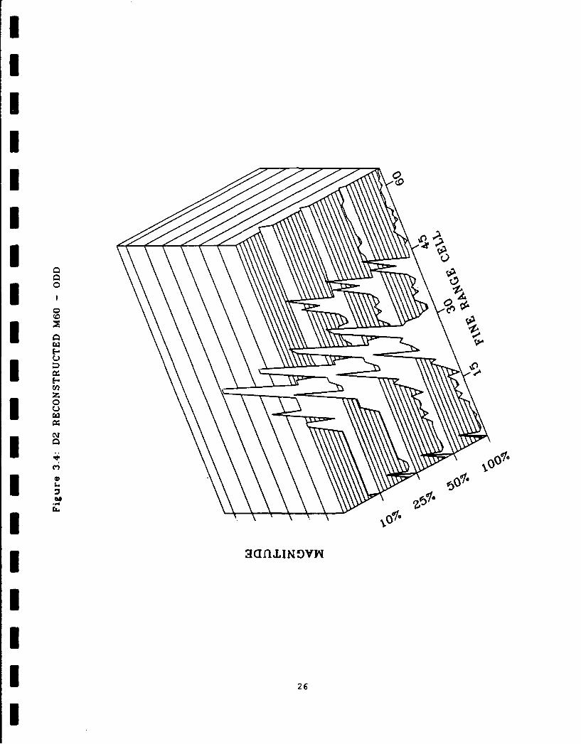
Typical (head-on aspect) HRRPs and partial waveletreconstructions using the D2 (Haar) wavelet basis and 50%,25%, and 10% of the coefficients to reconstruct the original(100%) HRRP are shown in Figures 3.3 through 3.6. Figure 3.3is a plot of the results for an even polarization M60 tank.Figure 3.4 is a plot for the odd polarization M60. Figure3.5 is a plot of the results for an even polarization M35truck. Figure 3.6 is a plot of the results for an oddpolarization M35. It can be seen from these figures that

21

I

reasonably fine structure is preserved along with the targetextent, even when only 25% of the wavelet coefficients areused to reconstruct the original target image. This reducestarget image dimension by a factor of four. It isconjectured that features from the reconstructed image may bemore robust than features from the original image. The nextphase of this contracc will investigate this conjecture indetail.

22

I0U0

EcJ

m :

I 000I C)I LLO

I 0.-

0)0

ID 23 15 I

* 0Cl)

Co CD)

.~

C/0

a-

4: 0

I~ 6: 0

I-

sC)

ICC0)0I I-wL

-J<* w L24

II

I-

0

&0

*2

IIIIIII

00

0CD

*0

*C,)z

C"

12C.,

I a.

I~Uf1JANDYN

III 26

I

III

IP

Cj

I2

......

IlPIcIzI0

cII(

I28

I

U 3.2 Wavelet Approximation to the FFT

Several studies were conducted using the radar data todevelop and demonstrate wavelet processing methods forapproximating the Fourier transform and extracting targetfeatures. The experiments ranged from simple demonstrations ofthe methods, which proved that they could be performed, to aseries of trials to evaluate the sensitivity of the methods to the

choice of wavelet basis functions and target signature variations.The sensitivity of these methods to the selection of basisfunctions is important, in part because the choice of basisfunction directly influences the computational complexity of themethod. The sensitivity to signature variation is important

mI because the military targets (i.e., tank and truck) exhibitsignificant signature fluctuations as a function of viewing angle.

This section reports the results of these studies which wereperformed to assess the basic feasibility of performing waveletapproximations to the discrete Fourier transform (DFT). Themathematical details of wavelet transform theory are discussed inAppendix B.1, and details of wave transform approximations toIFourier transforms are in Appendix B.2.

The method we chose to quantify the error of approximation isthe ratio of the mean squared error, to the total energy in thesignal. This method is sensitive to any loss of target energy bythe approximation method and the normalization allows the directcomparison of different signals.

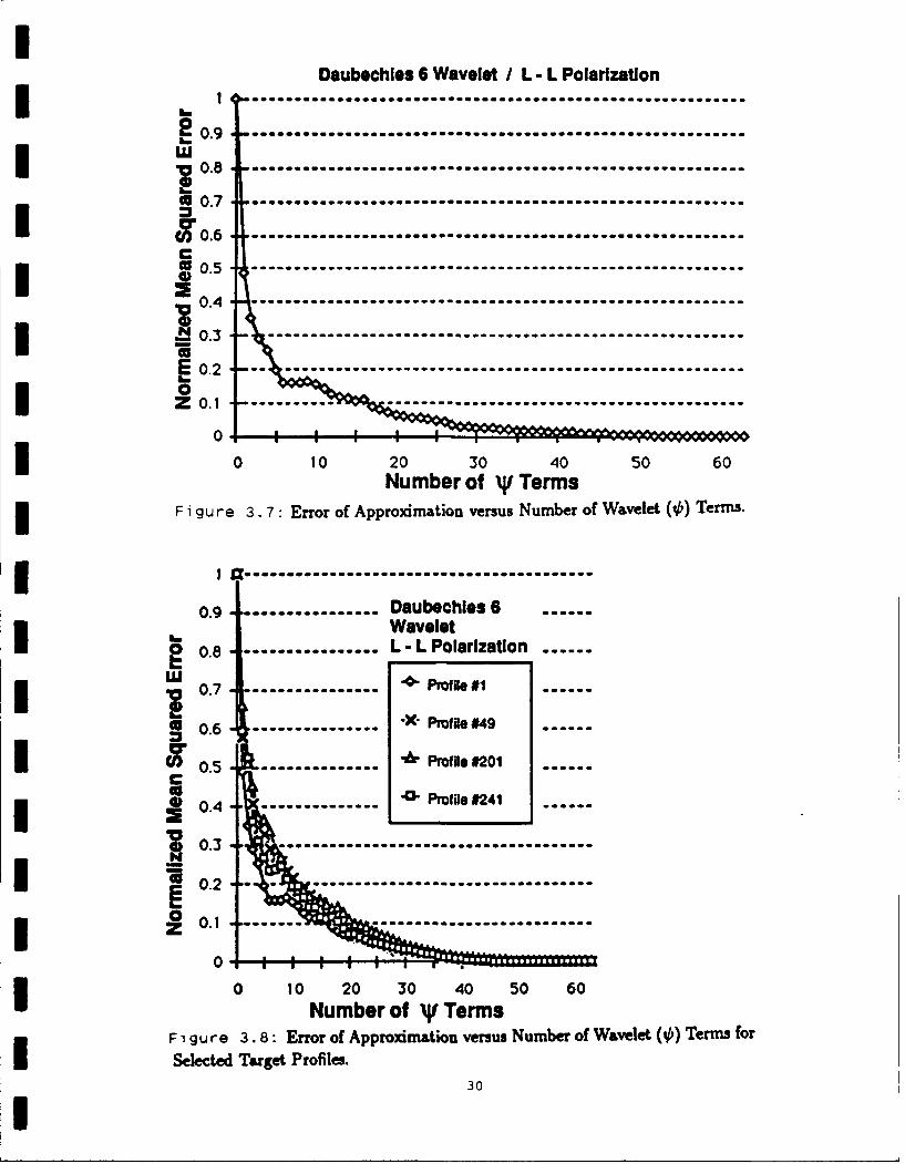
Figure 3.7 illustrates the normalized error of approximationas a function of the number of wavelet terms retained in thewavelet FFT approximation formula (B.30). Note that, for this M60tank scattering profile, the error of approximation decreases veryrapidly in the first 5 or 6 terms followed by a more gradual andsteady convergence to zero. This behavior is typical of themethod applied to other target profiles, as illustrated i±i Figure3.8. The convergence of this method for each of the targetprofiles (which vary in aspect or viewing angle) is rapid andconsistent. The method shows little sensitivity to changes inaspect angle and therefore to target signature variations.

Figure 3.9 is a plot of the error for a number of waveletbases. The functions considered ranged from a 2 coefficientwavelet basis (the Haar basis) to an eight coefficient waveletbasis (Daubechies - 8.) There is very little difference in theirperformance. This surprising result indicates that theapproximating wavelet basis does not have to be chosen verycarefully and that the computational advantages of short waveletscan be fully exploited in this application.

In the previous cases, the wavelet terms which were retainedin the approximation were the wavelet coefficients with thelargest absolute value. They were determined by sorting thewavelet coefficients. Sorting is an expensive computationalprocess which would quickly eliminate any computational advantagewavelets would have relative to Fourier methods. There is analternative formulation of the wavelet approximation to theFourier transform which uses all of the wavelet coefficients at agiven scale (Eq. B.33) rather than coefficients selected by

29

Daubechies 6 Wavelet / L - L Polarization11 ............................................

e 0.9 ---- --- --- --- --- --- --- ---- --- --- --- --- --- ---I w

40 0.7 -------------- -- -- -- --- -- -- -- -- --- -- -- -- --

C

E 0.2 -- - - - - - - - - - - - - - - - - - - - - - - - - - - - -0

00 10 20 30 40 50 60

Number of V~ TermsF i g u r e 3. 7: Error of Approximation versus Number of Wavelet ()Terms.

11 ----- ----- ----- ---- . . . -------- ---- .

0.9.............---Daubechles 6 ...WaveletI0 08 ---------. ---LLPoarization ......

07.............. Profile#21 ...XProfl #41

U 0.5 ------------------ Prfo#0 ...

0.4.... .........................

0~

0 10 20 30 40 50 60I Number of 41 TermsFi gure 3.8: Error of Approimation versus Number of Wavelet ()Term forI Selected Target Profiles.

30

0.9

2,0.8 ------- Target Profile #1-, L - L PolarizationV 0.7 ....... ...----

.. -X* Daubechies 20.6 .. . ... ...

-"- Daubechies 4U) 0.5 - - - - - - -

------ "<O D a u b e c h ie s 64) 0.4 ----------

4 Daubechis 8* 0

So.1 --- ...........................

0 10 20 30 40 50 60

i Number of AV TermsF i 9 u re 3. 9: L-jr-or of Approximation versus Number of Wavelet ()Terms for

Selected Wavel-t Bases&

1 m4 ----..s -- -- ....................------- ------------------- -----

* 0'

11 0.8 10.20.30 .4 . ......• SNDumber of em

a. 0.7 --- --- -- --- -- --- --- -- --- -- -. - --

I Z 39 ro of- DApproxmhtio vessNme8fWvlt( em o

U 0.9 .....................................

WO -le Polarization

!C

50.5*X* Daubechlos 2

*~0.4 ----------- .

N1& Daubeches 4= 0.3 ........ ...

102 Daubeciies:6

0 1 2 3 4 5 6Number of 4f Levels (J's)IF F g u re 3. 10: Error of Approximation versus Scale (tp) Levels for Selected

Wavelet Bases. 31

I

I magnitude. An experiment was performed to evaluate thefeasibility of eliminating entire scales from the approximation.Figure 3.10 shows the results for several wavelet basis functions.The approximation is very poor until the smallest scale waveletcoefficients are included. This means that the energy wasdistributed in wavelet coefficients across all scales.

The results of the previous experiment motivated a search fora method to preprocess the radar data so that the target energycould be placed into predictable scale levels and therebyeliminate the need to select (or sort) the most significantwavelet coefficients. This led us to adapt a method called "phaseunwrapping" to this problem. Appendix C describes themathematical details of the procedure. When it is applied to theradar data, the target energy is concentrated into the lowestscale levels and the approximation method can discard the highestscale level terms with little loss of information. Thissignificantly reduces the computational complexity of the method.Figure 3.11 illustrates the reduction in error it produced.

In conclusion, it is feasible to apply the waveletapproximation to the Fourier transform to the millimeter wavesensor problem of producing HRRPs. The error of approximation canbe controlled to any level desired by adjusting the number ofwavelet terms retained in the approximation. The computationalcomplexity of the wavelet methods for wavelet support lengths of 6or less are comparable to the Fast Fourier Transform for the radardata used in this study, which is processed in blocks of 63complex data points. The target data is contained in a relativelylarge fraction (1/2 to 1/3) of the output data points whichrequires that a large fraction of the wavelet coefficients beretained in the approximation. This increases the computationrequired for the wavelet methods. The target extent varies fromabout 10 fine range resolution cells to 30 range resolution cells.The error of approximation was about 0.10 (Norm. MSE) when 16terms were retained and was less than 0.05 (Norm. MSE) when 32terms were retained. It should be noted that the 8 termapproximations contain over 80% of the original target energy, buthave relatively severe "shape" distortion.

Since the wavelet methods offer no computational advantageand produce some error, they are probably not an appropriate

choice for this particular radar data processing problem due tothe small number of data points to process. However, if the datacame from, for example, an FMCW (with a long pulse length) thatperformed 1024 point FFT's, yielding one foot range resolution,tank and truck detections, which are 10 to 30 feet long, dependingon aspect, could be very efficiently processed by wavelet FFTapproximation. Additional comparison results are given inAppendix B.3.

32

U Without Phase Unwrapping

I 0.9 - -- -- -- --------- -- --- -V 0.8 -- - - - - - - - - - - - - - - - - -- - -

CC0. tmIp-----------------------------UI 0.6--------------------- ----------

I 2022 0.4 ------------- 6W a---e- ------

= 0. ---2-3--4-- 6

wrappedO Target Poie#

EI. abcle aeeIhI . o a ia io -- .....IZI0

I 33

I

i 3.3 Target Length Estimation

This section presents the results of experiments conducted onthe radar data to develop and investigate the capabilities ofwavelet based feature extraction methods. Of particular interestwas the feasibility of performing feature extraction with awavelet based approach and the stability of the method withrespect to target signature variations due to change of aspectangle.

The feature which was selected for analysis was target extentwhich is the length of the target image in the high resolutionradar range data. This feature is important because it requiresthat both the "front" and "back" of the target be determined.Target classification algorithms need this information to delimitthe region in the high resolution radar data which contains thetarget detail. The performance of the wavelet methods is comparedI to a baseline method described in appendix E.

The following procedure was used to measure the stability ofthe target extent methods.

I 1. Calculate the target extent for a large number of aspectangles. The entire target data sets available to thesubcontractor were used for the results presented in thisreport.

2. Divide the results into contiguous blocks of 50 items andcompute the average extent for each of the blocks. Thisis interpreted as the true target extent in thisneighborhood.

3. Calculate the differences between the extents calculatedin step 1 and the local averages calculated in step 2.From the differences, calculate the standard deviationfor each block of 50 estimates. This estimate of thestandard deviation (locally) is a measure of thestability of the method.

4. Calculate the mean and standard deviation of the localstandard deviations calculated in step 3 for the entire

i available target data set.

The wavelet algorithm used for extracting the target extentwas based on thresholding the squared modulus of the large scalecomponent of the one-sided wavelet transform of the complex radarimage. This is a method for removing noise from the target data.It has two variations depending on the order in which mathematicaloperations are performed:

* IWT(zk) 12

* WTI (ik) J2

where WT() indicates a wavelet transform and I 12 the squared* modulus.

34

I

N The first case requires the wavelet transform of complexFourier transform data while the second case only requires that areal wavelet transform be performed. The performance of thesecond method was found to be better, as well as less costly. Itis described below.

The thresholding procedure is similar to the method used inthe baseline method (described in appendix E) except that only onehalf of the number of high resolution range cells are used tocompute the noise floor because the one-sided transform componentsare sampled at half the original rate, i.e. they are half thelength of the original sequence. Two additional variations of thewavelet transform method were studied to investigate thesensitivity to scale. The one-sided wavelet transform method wasrecursively applied to the large scale components resulting indata which were sampled at 1/4 and 1/8 the original rate. Thesecases used only four and two high resolution range cells,respectively, to estimate the noise floor. The general waveletmethod used to estimate target extent is the following.

1. Compute the discrete Fourier transform (DFT) zk of thephase history data sequence Zk.

2. Compute the squared modulus of the transformed data i~k1 2 .3. Compute the large scale component of the one-sided

wavelet transform of i~k1 2 .

4. Establish a threshold T>O. (T became 25.)

5. Compute the average power A of the 8 (or 4 or 2) highresolution range cells furthest away from the target.Since the target is known to be located in the center ofthe range gate, these are the first and the last 4 (or 2

* or 1) high resolution range cells.

6. Compute the indices I, and 12 of the first and lastentries of I k1 2 that exceed T x A

7. Compute target extent as 2 x (12 -I1 + 1) [or 4 x (12 - 1l+ 1) or 8 x (12 -I1 +1)].

The computational cost in real multiplies of these threefiltering methods are (where K is the size of the wavelet system):

I 1. For the one half scale method:Cost(N) = (K+1)(N/2)O(N);

2. For the one quarter scale method:Cost(N)=(K+l)(3N/4)0(N);

3. For the one eighth scale method:Cost(N)=(K+l)(7N/8)I =(N).

I

I

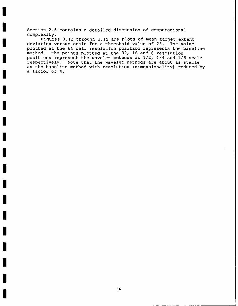
I Section 2.5 contains a detailed discussion of computationalcomplexity.

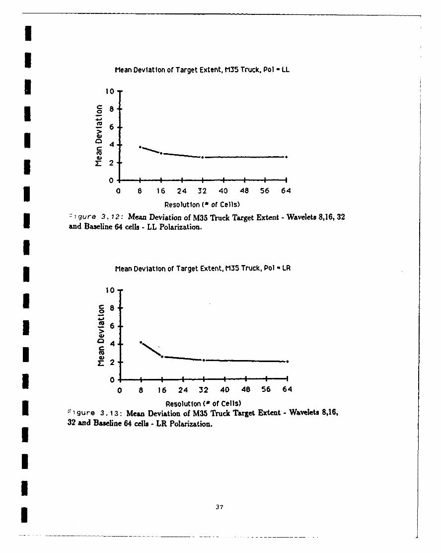
Figures 3.12 through 3.15 are plots of mean target extentdeviation versus scale for a threshold value of 25. The valueplotted at the 64 cell resolution position represents the baselinemethod. The points plotted at the 32, 16 and 8 resolutionpositions represent the wavelet methods at 1/2, 1/4 and 1/8 scalerespectively. Note that the wavelet methods are about as stableas the baseline method with resolution (dimensionality) reduced by

* a factor of 4.

IIiI

I3

I

NMean Deviation of Target Extent, M35 Truck, Pol -LL

* 10I ,I .I

-6

04

0 2

0 8 16 24 32 40 48 56 64

Resolution ( of Cells)1 gure 3. 12: Mean Deviation of M35 Truck Target Extent - Wavelets 8,16, 32

and Baseline 64 cells - LL Polarization.

IMean Deviation of Target Extent, M35 Truck, Pol LR

0I go8I

I 0 _ _

6 2

1 0o

0 8 16 24 32 40 48 56 64

I Resolution (# of Cells)U :1 gure 3. 13: Mesa Deviation of M35 Truck Target Extent - Wavelets 8,16,32 and Baseline 64 cells - LR Polarization.I

III

II

Mean Deviation of Target Extent, M60 Tank, Pol - LL

I 0

I-- o ......

0I I I,-I I

0 8 16 24 32 40 48 56 64

Resolution (I of Cells)Sigu re 3.14: Mean Deviation of M60 Tank Target Extent - Wavelets 8,16, 32

and Baseline 64 cells - LL Polarization.

I

UMean Deviation of Target Extent, M60 Tank, Pol - LR

S10

I6-4--I N-" " __

2 2

3 0 8 16 24 32 40 48 56 64

Resolution (* of Cells)i1 gure 3.15: Mean Deviation of M60 Tank Target Extent - Wavelets 8,16, 32and Baseline 64 cells - LR Polarization.

I

* 38

II

3.4 Wavelet Target Classification Results

I A two class target classification experiment wasconducted to see if it is feasible to improve radar targetclassification signal processing by wavelet methods, eitherby improving classifier percent correct classification (PCC)in the presence of noise (added to the very clean radartarget data) or by decreasing the number of computationsrequired by the classifier processor, or both. Theclassification problem examined was for two vehicles, an M60tank and an M35 truck. The tank might be a target for amissile, but the truck might be a target-like object that onewould not want to waste a missile on. Classifier overall PCCwas improved in realistic signal/interference situations byup to 6 percentage points, and computations were decreased bya factor of 10.

Quadratic classifiers were used with either odd degree(1,3,5,...) aspects as the "training" set and even degree(0,2,4,...) aspects as the "test" set or the reverse. Noisewas never added to the "training" set. Because this isactual radar data taken on an outdoor range with very lightclutter background, the "clean" data has a signal to clutterratio of greater than 20dB. The wavelet basis selected wasthe Haar or Daubechies 2 wavelet basis. The features used bythe classifier were particular wavelet coefficients producedby the target HRRPs. Wavelet coefficients were selectedlogically but by no means optimally.

Specific results are given in Figure 3.16. Theseresults clearly indicate that it is feasible to improve radarclassifier processors by wavelet methods.

This study used one odd polarization and one even

polarization. This would be the case if one transmitted onlyone of the two circular polarizations, but received bothcircular polarizations or the reverse. The starting pointfor this study was the target HRRPs, which contained one footrange resolution target magnitude data. It is assumed thattarget length (as seen by the radar) is no more than 32 feetIn reality, target length varies considerably depending ontarget aspect angle. For example, targets are longest whenviewed from a head-on (0 degree aspect) or from a 180 degreeaspect.

In Figure 3.16S = total signal powerN = total power of noise addedS/N given is for the tank (higher for the truck)HR54 = 32 odd & 32 even HRRP components

W64-11 = 11 coefficients from HR64 wavelet transform.As part of the next phase, it will be important to

perform a three class classifier experiment. This was notaccomplished during this phase due to cost and scheduleconstraints.

139

I Figure 3.16: Target Classification - Original vs. Wavelet

COMPLEXITY (number of multiplies)

HR64 2144

W64-11 = 205 (90% reduction)IPERCENT CORRECT CLASSIFICATION

S/N S/N(dB) HR64 W64-11zero noise 92 85

6.6 8.2 77 832.7 4.3 69 720.67 -1.7 59 60

I

I4

I

i 3.5 Fine Range Resolution by Wavelets

It is theoretically possible to obtain fine range

resolution HRRPs by using wavelet transforms instead of FFTsif the waveform transmitted is modified to be appropriate forwavelet transforms. This possibility is important becausea radar's digital signal processor (DSP) is typically one ofthe more costly parts of the radar due to heavy processing

load requirements - primarily due to the need to perform manyFFTs. Since a wavelet transform is considerably faster thanan FFT, significant DSP cost, weight, and size savings willresult from wavelet, rather than FFT, HRRPs.

A wavelet transform matrix W can be constructed from theproduct of a number of wavelet "butterfly" matrices. This issimilar to computing a discrete Fourier transform (DFT)matrix as the product of FFT "butterfly" matrices. Unlikethe DFT matrix, the wavelet matrix W consists of real (ratherthan complex) numbers, for the four wavelets of initialinterest, D2 (Haar), D4, D6, and D8. The column vectors, wi,W2, ... , wn of the n-by-n matrix W are orthonormal. If y

-- denotes the column vector of wavelet coefficients for aninput column vector x, then y could be computed by (moreefficiently by "butterflies")

y' = x' W (3.2)

and the absolute value of the components of y will be afine range resolution HRRP if the n transmitted waveformscorrespond to the wavelets in the following ways.

1. The n sequential transmitted waveforms look like the nrows of the matrix W. (The orthonormal waveletvectors are the columns of W.)

-- 2. The transmitted waveforms are "stretched" to twicethe W-row-length, n, to allow for 2-way travel.

An eight dimensional example with the Haar wavelet follows inFigure 3.17. The example easily can be extended to a 32 or

64 dimensional version. The Haar wavelet is easy toIdescribe, but due to it's non-smooth nature it is probablynot a good wavelet waveform for radar transmission. InFigure 17, instead of stepping frequencies from one waveformto the next, the shape of the waveform changes in a waveletrelated fashion. There are 8 wa.eforms used to break an 8foot long range bin into 8 one foot segments by wavelettransform (instead of FFT). The time duration of the

-- waveforms is 16 feet divided by the speed of light.There are two speed advantages to transmitting wavelet-

related signals and processing by wavelets to get fine range

I- profiles.

1. Wavelet transforms are O(n); FFTs are O(nlog2(n)).

2. D2, D4, and D6 wavelet transforms use 1-cycle

real*real multiplies; FFTs of I,Q data use 6-cycle

* 41

complex*complex multiplies (4 multiplies, 1 add,and 1 subtract)

Figure 3.17: Haar Waveforms for HRRPs

Wave # Waveform

1 _-

2 ---------

3 f

4

3 6

I 77

18 minK 7

8

* 42

I

4.0 Supplemental Results

Figures 4.1 through 4.3 contain plots of partial

reconstruction by D6 wavelets, of a normalized odd bouncepolarization HRRP from a radar look at the calibratedtrihedral corner reflector. Figures 4.4 through 4.6 containsimilar plots for an even bounce polarization HRRP from aradar look at two dihedrals that are separated by about 10feet in range. Each plot lists the number of terms used inthe reconstruction and the normalized mean square error.

Figures 4.7 through 4.10 show estimated target lengthversus aspect angle for the M35 truck. The polarization waseven (transmit left circular and receive left circular). Thefour plots are for FFT (Martin Marietta method) processing,wavelet reconstruction dimension reduction by a factor of 2,then 4, then 8 respectively. Similar results are given foran odd polarization (transmit right circular and receive leftcircular) in Figures 4.19 through 4.22. Since target lengthwill vary with target aspect, it was decided that a good

measure of length estimation stability would be the standarddeviation (over blocks of 50 radar looks) of the lengthestimate. That is, a small standard deviation would indicatestable length estimation. These results are presented inFigures 4.11 through 4.18 for an even polarization M35 truckand in Figures 4.23 through 4.30 for an odd polarization M35

truck. Figures 4.11, 4.13, 4.15, and 4.17 contain plots ofthe mean of the length estimates from blocks of 50 M35 looks.Figures 4.12, 4.14, 4.16, and 4.18 contain plots of thestandard deviation of the length estimates from blocks of 50

i M35 looks, along with a numerical mean and standard deviationof these standard deviations. This standard deviationcomparison was the figure of merit used to determine thestability of the wavelet methods.

Figures 4.31 through 4.34 show estimated target lengthversus aspect angle for the M60 tank. The polarization waseven (transmit left circular and receive left circular). Thefour plots are for FFT (Martin Marietta method) processing,wavelet reconstruction dimension reduction by a factor of 2,then 4, then 8 respectively. Similar results are given foran odd polarization (transmit right circular and receive leftcircular) in Figures 4.43 through 4.46. Target lengthstandard deviation versus aspect angle results for an M60tank are presented in Figures 4.35 through 4.42 for an evenI polarization M60 tank and in Figures 4.47 through 4.54 for anodd polarization M60 tank. During the analysis it wasdiscovered that a portion of the data for the M60 tank wasfound to be unusable. Although it was too late in theanalysis to determine the problem and supply the correct datato our subcontractor, it had no significant outcome on the

results.

For both trucks and tanks these results show waveletdimension reduction by a factor of 2 or 4 looks acceptablebased on a desire for small standard deviations, but when thedimension is reduced by a factor of 8 the standard deviation

43

I

becomes large and erratic. Consequently, the results showthat dimension can be reduced by up to a factor of 4 but not8, with no appreciable loss of stability in length esti-mati on.

III

I4

Number of terms =8 Normalized MSE = .4539350

* 300-

250

200

150

100

50

0 00 10 20 30 40 50 60 70

Figure 4. 1: Partial Wavelet Reconstruction-lihedral, N=[81.

Number of terms =1 6 Normalized MSE = .227700

600

500

400

300

200-

100

00 10 20 30 40 50 60 70

Figure 4.2: Partial Wavelet Reconstruction-Tihedral, N=[16].

45

Number of terms =32 Normalized MSE =0.007747I1200 1

1 1000-

800-

600-

400-

* 200-

010 10 20 30 40 50 60 70

F igu re 4. 3: Partial Wavelet Reconstruction-MNhedral, N=[32].

Number of terms =8 Normalized MSE =.3482450

I 400-

* 300-

250-

200-

1 150-

* 100

I 50

0-0 10 20 30 40 50 60 70

I ~F igu re 4 .4: Partial Wavelet Reconstruction-Dihedral, N=[8].

INumber of terms =16 Normalized MSE = .1441

800

* 700.

600

500

I 400

I 300

- 200-

* 100

m0

0 10 20 30 40 50 60 70

F i gu re 4.5: Partial Wavelet Reconstruction-Dihedral, N=[16].

I Number of terms =32 Normalized MSE = 0.0098671200

1000

800

* 600-

400

* 200-

I 00 10 20 30 40 50 60 70

F i gure 4.6: Partial Wavelet Recontruction-Dihedral, N=[32].

47

Fi gu re 4.7: Target Extent versus Aspect AngleTarget: M35. Threshold: 25, Polarizaton: LL

Analysis of Real data (Martin Method)

6 0 V

I 550-

40

2

1O I .l

20* 10

0-1-20 0 20 40 60 80 100 120 140

aspect angle

Fi gure 4.8: Target Extent versus Aspect Angle

Target: M35. Threshold: 25, Polarization: LLAnalysis of Real data (D6 Level 1)

60

Im 50

I 40

20

10

0-20 0 20 40 60 80 100 120 140

aspect angle

48

Figure 4. 9: Target Extent versus Aspect AngleTarget: M35, Threshold: 25, Polarization: LLI Analysis of Real data (D)6 Level 2)

60-

50

I t~40-

I J~30 I

~20 U

10

g ur0. 01a p c n leII H-20 0 20 40 60 80 100 120 140

Fiue4I0 Target Extent versus Aspect AngleTarget: M35. Threshold: 25. Polarization:~ LL

60 Analysis of Real data (1)6 Level 3)

50-

I 40.

S 301

> 20-

I 10-

0 I-20 0 20 40 60 80 100 120 140

aspect angle

I 49

Figure 4.11: Average Target Extent versus Aspect AngleBlock Size: 50. Target: M35, Threshol" 25, Polarization: LL

70 Analysis of Real data (Martin Method)

60

50

) 40

30-E

20-

10-

01Block #t 50 100 150 20250

gu re 4.1 2: Standard Deviation Target Extent versus Aspect Angle

Block Size: 50, Target: M35, Threshold. 25, Polarization: LL

Analysis of Real data (Martin Method)

18-

16-

14-

S 8-

6-

Block #t 50 100 150 200 250

mean = 2.563 s.d. = .7725

50

IIFi gure 4. 1 3: Average Target Extent versus Aspect Angle

Block Size: 50. Target: M35, Threshold. 25, Polarization: LL70 Analysis of Real data (136 Level 1)

I 60

I 50

S30-

20

0

Block # 50 100 150 200 250

SF igu re 4. 14: Standard Deviation Target Extent versus Aspect AngleBlock Size: 50. Target: M35, Threshold' 25, Polarization: LL

Analysis of Real data (136 Level 1)

18

16

14

" 12

c 10

*2

Block * 50 100 150 200 250

mnean=2.615 s.d. =.9637I 51

I F i gu re 4. 15: Average Target Extent versus Aspect Angle

Block Size: 50,Target: M35, Thrshold- 25.Polarizaton: LLI7Analysis of Real data (D6 Level 2)70

60

50

.~40-IC

I I o

Block 50 100 .150 200 250

Figure 4.16: Standard Deviation Target Extent versus Aspect AngleBlock Size: 50, Target: M35, Threshold. 25, Polarization: LL

20 Analysis of Real data (D6 Level 2)

H -

18

16

14

-Z 12

B 10U

. 8 8

6

* 4-

2-

01Block # 50 100 150 200 250

mean= 3.018 s.d.= 1.174

52

U Figure 4. 17: Average Target Extent versus Aspect AngleBlock Size: 50. Target M35, ThresholdL 25. Polarization: LL

70 Analysis of Real data (D6 Level 3)

60

50

.I 40

30O

20

Block # 50 100 150 200 250

I Fi gure 4.1 8: Standard Deviation Target Extent versus Aspect AngleBlock Size: 50, Target: M35, Threshod. 25, Polarization: LL

Analysis of Real data (D6 Level 3)

18

I 16

14-

12

.• 8

* 4

Block 0 50 100 150 200 250

mean = 3.794 s.d. = 1.698

53

I Figure 4. 19: Target Extent versus Aspect AngleTarget M35. Threshold: 25, Polanzaon: LRu 60Analysis of Real data (Martin Mediod)

I 50-

* 4 0

20

10-

01-20 0 20 40 60 80 100 120

aspect angle

Fi gu re 4. 20: Target Extent versus Aspect AngleTarget M35. Threshold: 25, Polarization: L.R

Analysis of Real data (D)6 Level 1)

* 60-

* 50-

I ~ 40-

I ~30

> 20

-20 0 20 40 60 80 100 120

I aspect angle

54

I Figure 4.21: Target Extent versus Aspect AngleTarget M35. Threshold: 25. Polarization: LR3 Analysis of Real data (D6 Level 2)

60

I50

I 40

530

0

-20 0 20 40 60 80 100 120

aspect angle

Figure 4.22: Target Extent versus Aspect AngleTaget M35. Threshold: 25, Polarization: LR

Analysis of Real data (D6 Level 3)

60

-* 30

U 2

10

01-20 0 20 40 60 80 100 120

aspect angle

55

F i gure 4. 23: Average Target Extent versus Aspect AngleBlock Size: 50, Target: M35, Thresokl 25, Polarizaton: Li

Aralysis of Real data (Martin Method)70

60-

50

S 40-

3 30

10

Block * 50 100 150 200

F i gure 4.24: Standard Deviation Target Extent versus Aspect AngleBlock Size: 50. Target" M35, Thmshokl: 25. Polarization: LR

Analysis of Real dat (Martin Method)

18

16

14

12

I ~10-

8

6

4

3 20

Block # 50 100 150 200

mean = 1.946 s.d. = .5128

56

H pFigu re 4. 25: Average Target Extent versus Aspect AngleBlock Size: 50, Target: M35, Threshold. 25. Polarization: LR1 70Analysis of Reaidata(D6 Level I)

* 60-

* 20

I ±40

Block * 50 100 150 200

Figure 4.26: Standard Deviation Target Extent versus Aspect AngleBlock Size: 50, Target M35, Threshold: 25. Polarizaton: LR

AnaysofReal daa (D6 Level 1)

18-

I 16

- 14-

S 12

I .~ 8

6-

I 4-

Block * 50 100 150 200

mean = 2.149 s.d. = .6251

I 5-7

Figure 4.27: Average Target Extent versus Aspect AngleBlock Size: 50, Trge M35. Threshold: 25, Polarizaton: LR

Analysis of Real data (D6 Level 2)70

60-

50

0E

20

Block 0 50 10 150 200

F igure 4.28: Standard Deviation Target Extent versus Aspect AngleBlock Size: 50, Target M35, Threshold: 25, Polarization: LR

20 Analysis of Real daa (D6 Level 2)

18

I1614-

S 12-

8IK6-

* 4-

2

0Block t 50 100 150 200

mean = 2.578 s.d. = 1.023

58

Fi gure 4.29: Average Target Extent versus Aspect AngleBlock Size: 50, Target M35, Threshold: 25, Polarizaton: LR

70 Analysis of Real data (16 Level 3)

60

50

.2 40

3-

10-20

Block # 50 100 150 200

Figure 4.30: Standard Deviation Target Extent versus Aspect AngleBlock Size: 50, Target: M35, Threshold: 25, Polarization: LR

Analysis of Real data (D6 Level 3)20

18

S16

14

" 12

I ~10-

* 8

6

4

* 2

Block $ 50 100 150 200

mean = 4.185 s.d. = 2.286

59

Figure 4.31: Target Extent versus AspectAngleTuget: M60. Tbshold: 25, Polxiziors L±

Analysis or Reall data (Manin Metiod)

60-

40-

U missing

110-.2D 0 20 40 60 s0 100 120 140

aspect angle

3Figure 4.32: Target Extent versus Aspect AngleTwet: MW, Thrushold. 25, Polwiza:m LL

60Anaysis ofRealdata(D6 Levell 1)

I j40-

MissigI 30

06

Figure 4.33: Target Extent versus Aspecd AngleTmect M60, Tlushol& 25. Polwinio ILL

Andyvs of Real dam (DL6 L 2)

6O-

I 50

* MissingS 30-

I20 Data

I i"

10

0 -A-

-20 0 20 40 60 80 100 120 140

aspect angle

Figure 4. 34: Target Extent versus Aspect AngleTwjei M60. bemshokl 25. Polwiuzia LL

Analysis of Real dat (M Level 3)

60

.2D 0 20 40 60 so 100 120 140

spect angle

61

F i gure 4. 35: Average Target Extent versus Aspect AngleBkck Size: S0. Tarp M60. Thmhol 25 P miation: LL

Anaysis of Rel dim (Muin Muhod)70

60

SO-

I 50-

Missing Data

0Block s 5o 100 .150 20 250

I F i gure 4.36-. Standard Deviation Target Extent versus Aspect AngleBlock Size: 50, Target M0, Th-eshold: 25, Polwinion LL

Anaiym (Real daa(Martin Medlwd)

I 16

14

. 12

I 10 Missing Data

6

I 4-

2

0-Block *50 100 150 200 250

mean - 2.869 s.d. - 1.247

1 62

NFigure 4.37: Average Target Extent versus Aspect AngleBlock Size: 50. Tapt~ M60. Thuld. 25. Pobrizio: LL

'70Anaysis ofReal data(D6 Leve 1)

* 50-

I ~40-

Missing Dama

0Block 50 100 150 200 250

3 F igur e 4. 38: Standard Deviation Target Extent versus Aspect AngleBlock Size: 50, Tvger M60. Thmhol& 25. Polariuaon: LL

Analysis of Real data (D6 Lzvel 1)

20

I 16-

14-

* 12-

10-i Missing Data

6-

U4* 2

Block 50 100 150 200 250

-en 2-955 &.d. 1.14

* 63

I Figure 4.39: Average Target Extent versus Aspect AngleBock Size: 50, Targe M6, Threhold: 25. Pciianios LL

i 70 Analysis of Rea data (D6 Level 2)I "50

_- 40

0 IUII

Block 50 100 150 200 250

F i gu re 4.40: Standard Deviation Target Extent versus Aspect AngleBlock Size: 50, Target M60. T rshold 25, Pabizam LL

Analysis of Real daa (D6 Level 2)i ~20 ..

18

14-

12

I j10-

0II II8

6

I 4-* 2

Block 3 0 100 150 200 250

Imean *3.417 sLd. =1. 114

64

I F igure 4.41: Average Target Extent versus Aspect AngleBlock Sime: 50, TargeL M60.71mahold, 2S.Poimizaion: LL

70 Analysis of Rea data (D6 Lzvei 3)

j 60-

50-

~40-

Block #so 100 150 200 250

Figure 4.42: Standard Deviation Target Extent versus Aspect AngleBlock Size: 50. Target: M60, Tbzshol&L 25, Polatizasiow LL

20Analysis of Real dams (D6L UMe 3)

I 16-

I 14-

10-i Missing Data

Is6 -

I 0Block 0 50 100 IS0 200 250

Imean =3.794 s.d.- 1.741

I 65

Figure 4.43: Target Extent versus Aspect AngleTwget MW. MmrshoZ 25, Nfariznsiou U

Analysis of Real dons (Mm* Meahod

30

Ii50

.O40

6) Missangl

30

I 501

1-20 0 20 40 60 s0 100 120 140

upa ange

* 66

IFigure 4.45: Target Extent versAspedtAnlgleTwpet MW. Thrshod. 25, Pokarzuos: LAI Anialysis of Real da (D6 Level 2)

I ~ 40-

IMissngS 30

0.I-2D 0 20 40 60 so 100 12D 140

aspect SP

Figure 4.46: Target Extent versus Aspect AngleTvao MW, Thnshodd. 25, Polmizuuioa LAAnalysis of Real data (D6 Level 3)

I 60

I so0

I4~ Missing

* 20 Dmz

I 101

I 20 0 20 40 60 s0 100 120 140

asec angleI 67

I Figure 4.47: Average Target Extent versus Aspect AngleBlock Size: S0, Tet M60, Thnahold 25. Polwinaro.: Lit

70 Analyui ofRed1 ( Ni. Medho)

I601I 50-

I j40-

I Missing Data

IBlock #50 100 IS0 200 250

I Figu re 4.48: Standard Deviation Target Extent versus Aspect AngleBlock Size: 50, Twget: MW, Threshokk 25. Polwirazom LAI Anais of(Real da (Mn Medbod)

j 14-

I 12-

12 - M issing D a mn

6

I 4-I 2

IBlock #50 100 1SO 200 250

meAn -2.173 s.d. =.7198I 68

IFigure 4.49: Average Target Extent versus Aspect AngleBlock Size 50. Twget M60.7Wwmhobk 25. Polwizam- LAIAaalyssofRml dama (D6 Levd 1)

I 50-

I Mising Dam

Block # 50 100 150 200 250

F iga~re 4.50: Standard Deviation Target Extent versus Aspect AngleBlock Size: 50. Target M60, Thrubokd 25. Potiarmo LA

20Analysis or ReWdata (D6 LeeJ 1)

I 16-

- 14-

'0 12-

I 1 0 Miig Dama

* 4

* 2

0Block 0 50 100 150 200 250

mean -341 s.d. - .7422

* 69

Figure 4.51: AverageTargetExtentversusAspectAngleiliwk Size: 50, Tvet: M60, Thuaold: 25. Powindow LRAs si oed dam (D6 Levd 2)

0 1m

!S-

3 -10-

* 1o0

I I

0Block s 100 150 200 250

F i gure 4.52" Standard Deviation Target Extent versus Aspect AngleBlock Size: 50. Tge: M460.7kwhokL 25.Polbrim LA

Arl yzs ft(R dmrn (* LWe 2)

18

16

14

.~12-

d

6

4 - -

3 2-0 Block 5 50 100 150 200 250

mam 2.722 Ld. - .9377

70

1Fi gure 4.53: Average Target Extent versus Aspect Angle

Block Size: 50, TwSget M60, tushod 25. Pindm, LR

0Analyis of Real dam (D6 Lvel 3)

I 60-

70

I ,o

, U

Block so 100 150 200 250

F i gure 4.54: Standard Deviation Target Extent versus Aspect AngleBlock Size: 50, Tagez M60, td.K 25.Polwizadoa: LRI Analysis of Real data (D6-Lvd 3)

16

I 14V 12-

10- MisLng Data

6

4 -

1 2-01

Block 50 100 150 200 250

In 1 4.404 x.(L 1.658"71

Appendix A

List of Symbols

D Ring of dyadic rational numbers:= {z:Z=m/20, m,nEZ,n >0)

R Field of real numbers.

Z Ring of rational integers.

Ip :- Multiplier for wavelet system. p E Z and p > 2.

[a] Wavelet Coefficient Matrix ("WCM").

= a ... aN.-1

Iwhere N is an integer multiple of the multiplier p.

If p = 2 then we write:

I [a] :- Wavelet Coefficient Matrix ("WCM").

ADGbl ... bN-)

N Number of columns in a WCM. N is an integer multiple of p.If p = 2 then N is even.

72

Appendix B

Wavelet Transform Theory

B.1 Wavelets and Wavelet Transforms

Most signals in science and engineering are modeled as mathematical func-tions for purposes of analysis. In order to separate or examine certain impor-tant features or characteristics of the signal, the function is often expandedin terms of basis functions that span the space or a subspace that the sig-nals of interest reside in. The most common example of this is the Fouriertransform where a signal that originates in the time domain is reformulatedin the frequency domain by expanding the function in terms of trigonometricor complex exponential basis functions. This basis is most appropriate whenthe signals have periodic components or are produced by systems that aremodeled by constant coefficient differential or difference equations.

Consider a periodic, possibly complex-valued, signal g(t) that is squareintegrable over the range f 0< t _< 1 ) and with period one so that

g(t) = g(t + I). (B.1)

IThis function can be expanded in a Fourier series of the form

(t) =._ b, e'" (B.2)IM0with the coefficients given by

b, = j 9(t)e -'Un dt (B.3)

II

I 73

t

which is an inner product of g(t) with the basis functions. Similarly, oneIdefines the wavelet transform with respect to a basis of wavelet functions.The wavelet basis is generated by a p x N matrix [a] , where p and N

are positive integers and N is a multiple of p. The matrixI i S, .... aN,_I

I [a] aj.i(B.4)

Ior ... /

is a wavelet coefficient matr ("WCM") if it satisfies the scaling conditions

N-iI aka+ d =---- j.,(.k=O

I a= ,o, (B-6),

where bij equals I if i = j and 0 otherwise. The overbar denotes complexconjugation and I is an integer. The sums over k are finite sums since onlyfinitely many of the numbers a are different from zero.

The positive integer p is called the multiplier of the wavelet system andN is called its length;

This matrix of numbers provides coefficients for the vector of recursions

N-i

'[a](z) = > a'0[a](2z - k) (B.7)

which implicitly define the wavelet scaling function r0 [a] and explicitly definethe basic wavelet functions W'[a](z), 1 < i < p. Observe that only 0 [a]appears on the right hand side. The functions 0'[a](z) are defined for all realnumbers z E R.

The fundamental fact about systems of compactly supported wavelets isthat the collection of functions

Bauis[a:] {p:I2=p[aJ(pjz k)

o<i<, j,7,4z}

"74

form a basis for L' spaces, in particular for L2(R).We now focus on the case of p = 2 and will use the following simplified

notation for the scaling function jp(t) = 0 (a](t) and the wavelet function0t) E Jo'[a](t) where t E I. It can be shown that if the coefficients of thisequation satisfy the wavelet conditions, stated above, the solution W(Q) willbe orthogonal to integer translates of itself and can be normalized such that

< p( t ),,( t - k) > - I j(t) jp(t - k) dt = bok (B.8)

This means the set of basis functionsI ,(t) = i(t - 1) (B.9)

spans a subspace Vo in L2 and the coefficients of an expansion within thissubspace can be calculated as simple inner products. The feature of scalingfunctions that makes them attractive for signal processing is their ability tomodel signal properties that are related to the independent variable t. Onecan increase the size of the subspace spanned by the scaling functions byusing Wpjk(t) := 2 i/2w( 2jt - k) which spans a subspace V. One can show

I that VoCV 1 CV2 C---.The features of a signal can often be better described by defining a slightly

different set of orthogonal basis functions that span the differences betweenthe spaces spanned by the various scales of the scaling function. These newfunctions are the wavelets. The basic wavelet is defined in terms of the scalingfunction by

t = E"(_1)kaN-_k W(2t - k). (B.10)Is

It is the prototype of a class of orthonormal basis functions of the form

,jk(t) = 2"/2 ,(2it - k) (B.11)

where 2' is the scaling of t. 2-k is the translation in t, and 21/2 maintainsthe unity norm of the wavelet. We shall say that j is the base-2 logarithmof the scale. If W, is the subspace of L - L(R) spanned by the integertranslates of the wavelet 2/ 20,(2t), additional disjoint subspaces are spannedby integer translates of the wavelets for each different scale index j, that is,by the functions Ojk(t). The relationship of the various subspaces can beseen from the following expressions:

o C V C V2 C... CL 2 = L2(R), (B.12)

I

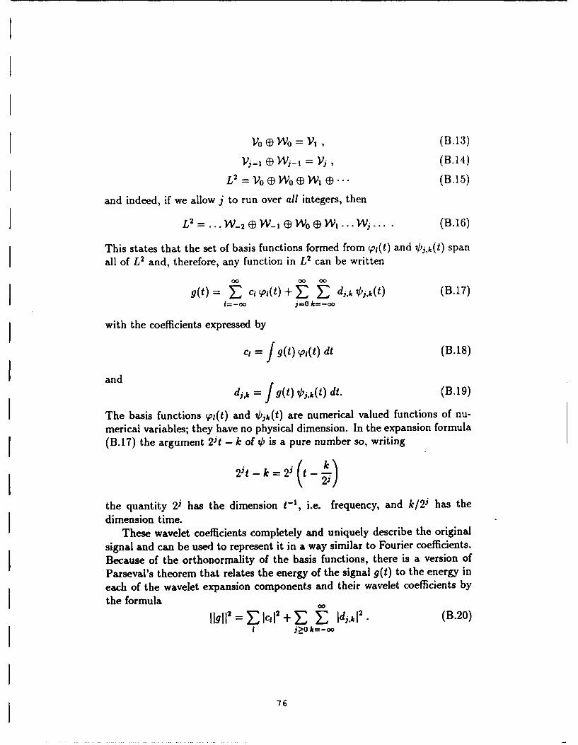
Vo (D Wo = Vi , (B.13)

Vj, E Wj,- = Vj, (B.14)

L 2 = V0 Wo( W 1 " (B.15)

and indeed, if we allow j to run over all integers, then

L 2 =...W-2 ED W-1 ( WO (D W....Wj... (B.16)

This states that the set of basis functions formed from p(t) and ,j,k(t) spanall of L2 and, therefore, any function in L2 can be written

g(t) = c pt(I(t) + E dj,k~ j,k(t) (B.17)1=-o j=O k=-oo

with the coefficients expressed by

= f g(t) pj(t) dt (B.18)

and

dj,k = I g(t) oLj,k(t) dt. (B.19)

The basis functions WI(t) and bjk(t) are numerical valued functions of nu-

merical variables; they have no physical dimension. In the expansion formula(B.17) the argument 2Jt - k of 0 is a pure number so, writing

2'i-k=2j t- _)

the quantity 2i has the dimension t-1, i.e. frequency, and k/2j has thedimension time.

These wavelet coefficients completely and uniquely describe the originalsignal and can be used to represent it in a way similar to Fourier coefficients.Because of the orthonormality of the basis functions, there is a version ofParseval's theorem that relates the energy of the signal g(t) to the energy ineach of the wavelet expansion components and their wavelet coefficients bythe formula 0011gll = E Icil + E Z IdF ,. (B.20)

I j>O k=-00

76

This is one reason why the orthonormality is so important. Daubechies [2]showed that the translates of the scaling function and the translated dilationsof the wavelets are orthonormal, and all of the these functions have compactsupport (i.e. are non-zero only over a finite region) if there are only a finitenumber of non-zero coefficients ak in the recursive scaling equation (B.7).This provides the time localization that is particularly desirable for analyzingboth the time and the frequency behavior of transient signals.

Note that there is an infinite set of scaling functions and wavelets thatcan be obtained by choosing different coefficients ak in (B.7).

B.2 Wavelet Approximation to the FourierTransform

In this chapter we state the relationships between the wavelet transform andthe Fourier transform as derived by Resnikoff and Burrus [5].

In this section we restrict attention to periodic functions g(t). Let mboxg(t+1) = g(t). Then the scaling function and wavelet coefficients in (B.18) and(B.19) are also periodic. The scaling function coefficients c(l) calculated from(B.18) and using (B.1) are

= 0 j V~(t - 1) g(t) dt 00 L p(r) g(Tr + 1) dr _= 0 p)g ( B.21)=Cov

W v

W w(].21)

Using the "partition of unity" property of scaling functions which states

00F, t- 1 (B.22)I 1=-ao

we can write (B.21) as

-- = f o(r-)g(r)dr= g(r) 1)o(r-L)df g(= dr =c.

"1-1(8.23)

Therefore, c is a constant and not a function of 1. Note the interestingproperty of W(t) which causes the scaling function coefficient of a periodic

I_ 77

function to be equal to'the DC Fourier series coefficient for any scaling func-

tion satisfying (B.7);

Lo V(t) g(t) dt = j g(t) di. (B.24)

Using the partition of unity property (B.22) again shows the scaling functionterm of the expansion in (B.17) is a constant.

~C1 ipt(t) = C ip(t - 1) = C. (B.25)I I

In a like manner, using (B.19) we calculate the wavelet coefficients in theexpansion (B.17) by

d,,k+K = 21 2 1 0(2it - k - K) g(t) dt = 2j/2 1 0(2'(t - 2-K) - k) g(t) dt(B.26)

which, after the change of variables r = t - 2jK and I = 2-jK or K = 2il,becomes s dj+ = 22 1 i,(2T - k) g(r + 2-jK)dT f dik. (B.27)

This statesdjk = dj.k+2,, (B.28)

or, the wavelet coefficients dj,, are periodic in k with period 2j. We nowuse these properties with the basic definition of the Fourier series coefficientsfrom (B.3).

b. = j g(t) e- '2 "" dt (B.29)

Substituting the wavelet expansion from (B.17) for g(t) into (B.29) gives

b. C if n = 0;b..= "00 "-'i , (,) in, 0(B.30)

Ejco Ej-dk~j~n)inn96O

where t(f) is the Fourier transform of O(t) defined by(f) -/0~~,p(t) e-i21 dt (B.31)

78

with an inverse given by

0(t) = I' ( f) "e'df. (B.32)

An alternative form, which uses the Fourier transform of the basic waveletk(t) rather than 0tj,,(t), is [5]:

C if n =0;

,j/2 i n 0 (B.33)Ejo0 2-/ djn) (2)in

where j(f) is the discrete Fourier transform (DFT) of dj,k for various scalesj and is defined by [1]

N-I

d,(rn) - ~ ~E, 2P "4kIN (B.34)k--O

with an inverse given by

1,, N-I irkN= -i dj(m) e2ik/N (B.35)

The formula for expressing the wavelet coefficients in terms of the Fouriercoefficients is easily obtained. From (B.19) we have

dj.k = g(t) Oj,k(i) dt.

which, after using (B.2) and reordering, gives

=i~ b,. 10 e' O"jk,(t) dt (B.36)

Godjk=- (B.37)

and, from (B.24), the scaling function coefficient is given by

ck = bo = c. (B.38)

79

An alternative derivation of (B.37) is

di,k = DTFT {b(6 ) n (B.39)

where the discrete-time Fourier transform is defined by

DTFT{z.) = i(f) = z - " (B.40)

and the inverse is=, L = ()•e 2"flI df. (B.41)

These are the basic relationships between the Fourier transform and wave-let transform. Equation (B.33) relates the Fourier series expansion coeffi-cients of g(t) to the Fourier transform of the fundamental wavelet and theDFT of the wavelet expansion coefficients of g(t). Equation (B.39) expressesthe wavelet expansion coefficients of g(t) in terms of samples of the DTFTof the product of samples of the Fourier transform of the basic wavelet andthe Fourier series coefficients.

In practice, a band limited signal sampled at the appropriate rate impliesa finite sum in (B.33) that corresponds to the finest scale of j = J and theFourier series is likewise finite. The independent variable f is frequency inHertz or cycles per second, d(m) is periodic with period N = 2j, and 1(f) isperiodic with period one. Clearly, the DFT or its inverse can be calculatedwith the FFT [1].

Energy and Parseval's Theorem

Orthonormal basis systems allow direct calculation and interpretationof the energy in a signal partitioned in both the time and the expansiondomains. Parseval's theorem for the Fourier series (B.2) states

a g(t)l2 d, = E Ib12. (B.42)

The "power" in a signal is proportional to the square of the signal (e.g.voltage, current, force, or velocity) and, therefore, the energy is given bythe integral of the square of the signal magnitude. Parseval's theorem states

80

how the total energy is partitioned in the frequency domain in terms of thepartition provided by the the orthonormal basis functions. For the generalwavelet expansion of (B.17), Parseval's theorem is

Lq(t)12 di- Ic1l2 + Go 0 12 (B.43)i--co j-O kw-oo

with the energy in the expansion domain partitioned in time by I and k andin scale by j. For the case of periodic functions, the relationship reduces to

J0 Lq(t)12 dt = IciI2 + OO 2j (B.44)

j=0 k-1

One can show that 1 (f)I --+ 0 as f -- 0 and also as f --+ o. Therefore,there will be a band of frequencies where most of the energy in (f) isconcentrated. Likewise, for many signals, the energy will be concentrated ina region of the (j, k) plane. Because of this concentration and using (B.33),the energy of the signal g(t) at frequency n and at scale j and time k isapproximately measured by

I2-j 1& (_I) 12jd, 12 (B.45)

If most of the energy in (f) occurs around frequency fo, then fo = n/2 j

relates the dominant Fourier frequency fo to the dominant wavelet scale j.Scale and frequency are independent primitive concepts, but the selectionof a wavelet basis establishes a connection between them, and the results ofthis chapter allow one to move between the two descriptions, using the onemost appropriate for a particular problem. The simple partitioning of theenergy content of a signal among frequencies has been generalized to includethe parameters of time and scale. In addition, we have at our disposal thechoice of wavelet systems, which is controlled by the choice of ak in (B.7),and determines the detailed nature of the relationship between frequency andscale.

I

B.3 Computational Complexity of the Wave-

let Approximation to the Fourier Trans-form

This section is concerned with the computational efficiency of wavelet-basedapproximations to the Fourier Transform. The computational cost for severalwavelet approximations of the Fourier transform are presented and compar-isons are made with the computational complexity of the FFT.

In the most applications, the size of the data set is the determining factor.We will refer to a technique's asymptotic complexity as representative ofhow quickly the number of computations grows as the problem size, N, in-creases. Comparisons with the FFT are natural here, since the FFT is acommonly used and well understood algorithm. We consider wavelet trans-forms which resolve to sub-band frequency components in part or perhapsall of the signal bandwidth. No attempt will be made to assign a value to aparticular scheme, since the level of approximation appropriate for a givenapplication can only be determined by extensive experiments. The quality ofthe approximation varies from approach to approach, and many simple andconsistent optimizations can be made, but usually require specialization toa particular set of circumstances.

The simplest, and also least accurate technique for estimating the DFTof a signal is a direct, balanced tree approach with filters optimized for sharpout-of-band rejection. Typically the Daubechies wavelets are used for thisapproach, although slight improvements in the quality of the results are pos-sible with other choices.' The computational complexity of pure waveletmethods are analyzed in section 2.5.

Additional improvements in the quality of the results and the speed ofcomputation is possible when full frequency resolution within a limited sub-

'Real wavelet filters have spectral characteristics which are conjugate-symmetric, andthese would combine large and small frequencies in the same band. To avoid this aliasing,a modification was made to the analysis and synthesis filters. Simply put, the filtercharacteristics were "rotated" so that, for a full bandwidth complex signal, whose Fouriertransform has the full 2N degrees of freedom, the low-pass side of a single analysis stagecaptures the lower half of the spectrum and the high pam the upper. In the real can,the Fourier transform is conjugate-symmetric, the "full bandwidth amounts to only f./2,half the sample rate, and "low-frequency' is then interpreted as being f./4.

82

band is the desired result. This is accomplished by using the wavelet trans-form to separate sub-bands, and then using an FFT on the data within theband to reconstruct a "local" approximation to the "full" Fourier transform.This can be done either (1) solely within that band, or (2) throughout theentire bandwidth. If the sub-bands used in such a reconstruction capturea significant fraction of the total energy contained in the signal, excellentapproximations can be constructed quite cheaply. Notably, the locations ofj peaks within bands are properly located and reconstruction away from edgesof sub-bands is quite accurate. The complexity of such a technique is:

I OPS = a(K)N(1 - R) + NR(3 + log(NR)) + RN (B.46)

where

I* N = the number of data points;

9 K = the size of the wavelet filter (assumed to be constant throughoutthe procedure;

* R = the portion of the bandwidth of the signal which is resolved (as-sumed to be 1/2L for some L).

For this estimate we assume that the reconstruction is done purely in-band,and only a single band is used (i.e., we don't expand further than necessaryto locate the energy, since that is wasted work if we truly want the DFT).

Figure B.2 shows the results of this calculation superimposed on the re-sults for a straight wavelet approach. The tightly clustered lines representthe hybrid case, and clearly show a usable advantage (i.e., reasonable lengthfilters are justified) over both the FFT and the straight wavelet methods for

problem sizes starting around 64 data points.In addition to the results stated there we note that significant improve-

ments may be made by combining these methods with phase-unwrapping inorder to move the "mass" of the return to the region of best filter perfor-mance, namely zero frequency for real filters and f = f./4 for the "rotated"filters.

The approach of relocating the center of the "target" frequency band isthe essence of the phase unwrapping technique, where the centroid is movedto the center of the DC or zero frequency band. Real Daubechies wavelets

83

Figure B.1: Tree Structure for the Hybrid Wavelet-Fourier Transform

Method.

84

16 HYBRID

14- 0.05

12.- 0.10

10....... 0. 15...... .... *..~... .. o

.. ....... ............... 0 .2 0

0.256 ""-:' ' ..................

6 ..... -- -- -- -- -- -- -- -- -- -- -- -- - 0.40

4 - . .0.50

100 101 102 103 104 lOs

Number of Data PointsFigure B.2: Computational Complexity of the Wavelet Transform vs. theFFT: Filter Length vs. N for equivalent complexity for various fractions ofthe total bandwidth (R) with the addition of the case when the FFT is usedto perform the final frequency analysis in a subband

have optimal performance at D.C and minimum aliasing. Phase unwrap-ping carries an overhead of N complex multiplies per N input points. Inaddition, calculation of the FFT for in-band components takes R additionaloperations while calculation of the entire FFT from inband components takesapproximately N additional computations. Neither of these has a significantcontribution to the total computation for large problem sizes, since both areoverwhelmed by the O(n log2(n)) behavior of the DFT's. The number ofoperations is then:

OPS = N + RN + aN(I - R) + NR(3 + log(NR)) (B.47)

85

16

14 R=.5

12 -- "

Me10 -

6--4-

2-V

0s

1 0 0 1210 041-

Number of Data Points

Figure B.3: Computational Complexity of the Wavelet Transform with PhaseUnwrapping vs. the FFT: Filter Length vs. N for equivalent complexity forvarious values of R for the case of using phase unwrapping and the FFT toperform the final frequency analysis in asubband

86

Figure B.3 shows the trade-off between this method and an FFT on thefull problem, reflected in the allowable filter size for equivalent quantities ofcomputations.

87

Appendix C

Phase Unwrapping

In this section we describe a method for preprocessing MMW radar data toconcentrate the target energy into the largest scale wavelet coefficients. Itis called phase unwrapping. It can be used to process radar fine range datafrom phase history data sequences whose bandwidth is less than one half thesampling rate.

This section has the following objectives:

" to describe the phase unwrapping algorithm

" to describe a method of radar imaging based on combining phase un-wrapping with the one-sided "Mallat" algorithm

" to present numerical examples using actual radar phase history data

The phase unwrapping algorithm is based on the topological concept ofwinding number. Let z : [a, b --o C be a differentiable complex valuedfunction. Define the winding number of z over the interval [a, b] by

W(z, a, b) = J Real(w(t)/z(t))dt, w = dzlidt. (C.1)

Hence W(z, a, b) represents the amount of angular winding about 0 (inthe counterclockwise direction) of the point z(t) as t moves from a to b. If z(t)represents (interpolated) phase history data formed from a rough reflector(several scatterers per resolution cell) then it is generally understood thatz(t) may be approximately modelled by a complex Gaussian random process

88

Radar Centrold60M60 Tank, L- L Polarizaon

. 50

~40

30

20

10

0 200 400 600 800 1000 1200 1400 1600 1800Record Number

Figure C.1: Radar Centroids for M60 Tank Target

having power spectral density function I(y). Furthermore, I represents theexpected value of li(y) 2 where i denotes the Fourier transform of z.

The expected value E(W) of W(z, a, b) equals 2r(b-a) times the centroidof I, thus E(W) = 2w(b - a) J I(z)z dz/ J I(z) dz. (C.2)

The factor 2r arises because of its appearance in the definition of the Fouriertransform.a The radar centroids and phase centers were calculated for 2000 differentaspect angles of the M60 tank target to evaluate the stability of the phase un-wrapping algorithm. Figure C.1 plots the results of the centroid calculationsand figure C.2 plots the results of the phase unwrapping method. Statisticalanalysis of these two sets of data reveals that the mean difference is 0.33range cells and the standard deviation of the difference is 1.32 indicating aslight bias but otherwise very consistent results. The correlation coefficient rbetween the two sets of data is 0.9986 indicating that the phase unwrappingmethod is a near perfect predictor of the true radar centroid.

I The phase unwrapping algorithm consists of two parts:

1. estimate the total phase winding of a phase history function z(t) fromits sample values zk,

2. remove this phase winding by multiplying z& by an appropriate complexsinusoidal sequence.

89

6o Phase CenterM60 Tank L- L Polaitation

50

t 30

10

0 200 400 600 800 1000 1200 1400 1600 1800ReCord Number

Figure C.2: Phase Centers Calculated by Unwrapping Method for M60 TankTarget

30. 1200

20 1000

10So

-10 400-2 2t~t 00

-30 - 4 aI OL11 I 9N10 10 20 30 40 50 60 0 to 20 30 40 50 60

Had Compowtit Modulus of Fouier Transfrm

Figure C.3: Raw Range Data and DFT for Trihedral Target

30. 1200

20-0

10. 600

-0 400

-20- 200

-30-t l 01 11 ~ 01I-IS4m4S0 10 20 30 40 so 60 -30 -?O.,_, .o, , , 30

R (Routed by 30 oile)

Figure C.4: Phase Unwrapped Data and DFT for Trihedral Target

90

*20 _ __ 200,1010 0

0 10 iL c4o 50 6o 0 30 40 50

Figure C.5: Raw Range Data and DFT for M60 Tank Target

30, 200

20

-10

-20-30 1 . . . . . . . . I . 0

0 10 0 so 60 -30 -20 -,0 0 ,0 20 30Modulus of FouulMe Tmosorm

(Rotsad by 30 calls)

Figure C.6: Phase Unwrapped Data and DFT for M60 Tank Target

I The first step requires estimating W(s, a, b) 'k=&-7 W(z, k, k + 1) fromsample values zk under the assumption that the bandwidth of z(z) is lessthan half than the sampling rate. In this case either zk or (-1)kzk is a lowfrequency content signal dk. Let ak denote the angle change between dk+l anddk. Then the average magnitude of ak is less than 90 degrees. This criteria3 can be used to select d = z, or d = (-1)"zk. Furthermore, ak (nearlyalways) represents either W(z, k, k + 1) or -7r/2 +W(z, k, k + 1). Therefore,W(z, a, b) " I.ak if dk = zk else W(z, a, b) z (b -a)r/2 - ak. Let

W denote the total phase winding.The second step consists of multiplying zk by the sequence e- w/(b - ) to

obtain Sk = zke - w / (' - ° ). By the assumptions on zk and by (C.2), Sk has alow frequency content.

To form a radar image from Zk apply the following steps:

I

*!9

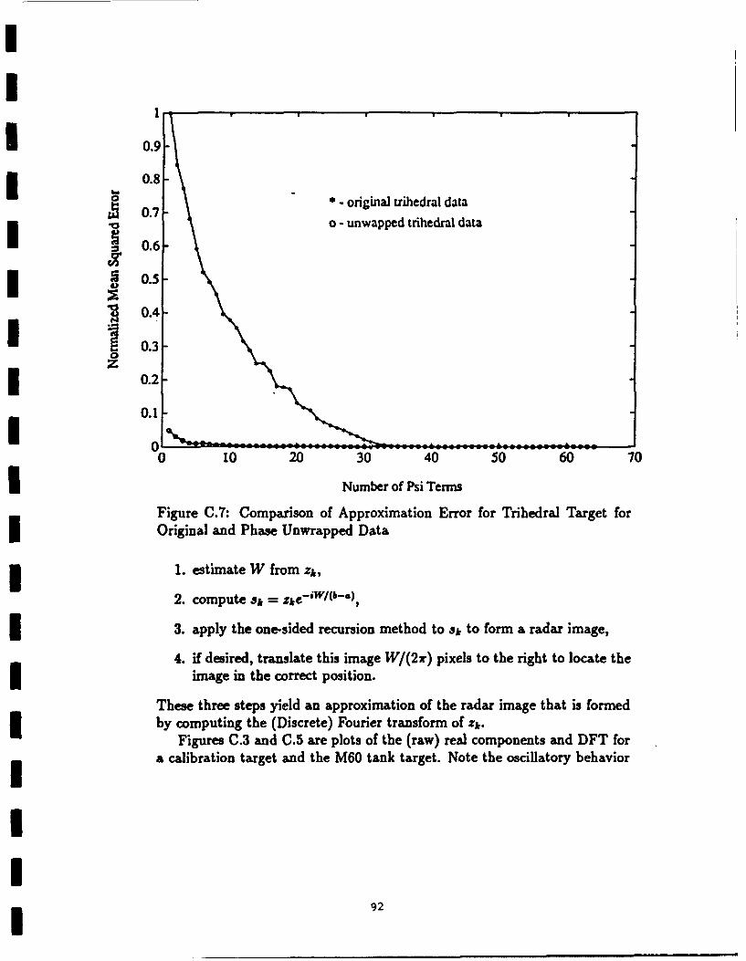
II

*_ 0.9

0.8-0.8- original trihedral data

0.7 o - unwapped trihedral data

I 0.6-

I ~ 0.5-

0.4-

I0.3I 0.2

0.1

0 10 20 30 40 50 60 70

Number of Psi Terms

Figure C.7: Comparison of Approximation Error for Trihedral Target forOriginal and Phase Unwrapped Data

I. estimate W from zk,

2. compute Sk = zke - iw l(&- ),

3. apply the one-sided recursion method to Sk to form a radar image,

4. if desired, translate this image W/(2r) pixels to the right to locate theimage in the correct position.

These three steps yield an approximation of the radar image that is formedby computing the (Discrete) Fourier transform of zk.

Figures C.3 and C.5 are plots of the (raw) real components and DFT fora calibration target and the M60 tank target. Note the oscillatory behavior

92

I

I

* 0.9

I 0.8-3.- original dihedral data

w 0.7 o - unwapped dihedral data

S0.6-

I 0.50.4

* 10.03

1 0.1

0-0 10 20 30 40 50 60 70

Number of Psi Terms

Figure C.8: comparison of Approximation Error for Dihedral Target for Orig-inal and Phase Unwrapped Data

93

of the raw radar data. The results of "phase unwrapping" the radar data forthese targets are presented in figures C.4 and C.6. In these figures note thedramatic reduction of oscillatory behavior which allows these function to bewell represented by only large scale wavelet terms. There is essentially noloss of shape information caused by the phase unwrapping process indicatingthat it can be used to reduce the computational complexity without addingany significant artifacts.

9

III

II

Appendix DI

Martin Marietta Radar DataI and Pulse Compression

I ProcessingI

This section examines the problem of radar range profile processing thatmay be amenable to solution by employing wavelet analysis in addition to orin place of conventional Fourier-based analytical methods. The unclassifiedradar detection processing problem is discussed in detail by Einstein [3] and

SSkolnik [6].The problem of obtaining sufficient target signal-to-noise ratio for MMW

radar systems with low transmitter power is solved by increasing the durationof the transmitted waveforms, thereby increasing the transmitted energy.Conventional "pulsed" radar systems have their range resolution determinedby the pulsewidth of the transmitted waveform and increasing the pulsewidthreduces the range resolution. This limitation is overcome by coding thetransmitted waveform such that processing (i.e., matched filtering) in thereceiver can recover compressed pulse information with an equivalent pulseduration approximately equal to the reciprocal of the spectral bandwidthof the modulated long pulse duration waveform. There are several pulsecompression methods available (see [6], §10) however, here we will focus onthe problem of processing time-frequencrcoded waveforms.

9

I 95

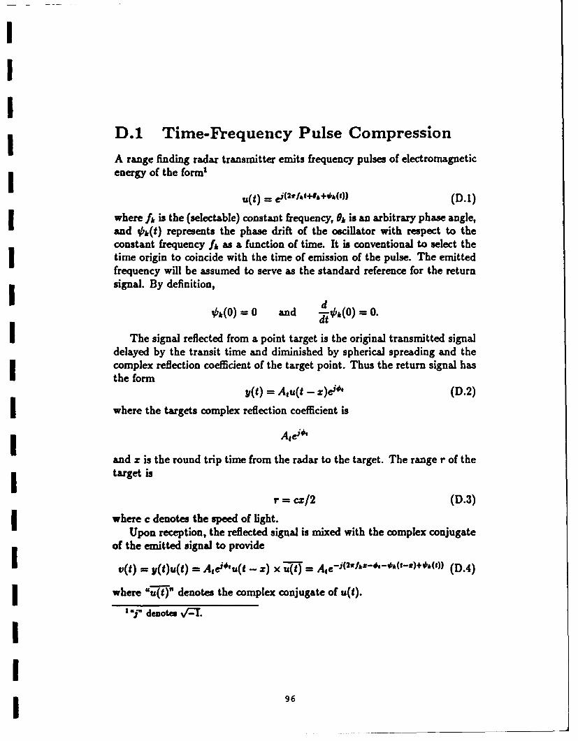
D.1 Time-Frequency Pulse CompressionI A range finding radar transmitter emits frequency pulses of electromagnetic

energy of the form'

u(t) =-(..+..() (D.1)

where fk is the (selectable) constant frequency, ek is an arbitrary phase angle,and Ok(t) represents the phase drift of the oscillator with respect to theconstant frequency fk as a function of time. It is conventional to select the

time origin to coincide with the time of emission of the pulse. The emittedfrequency will be assumed to serve as the standard reference for the returnsignal. By definition,

! k() = 0 and kk(O) = 0.dt0

IThe signal reflected from a point target is the original transmitted signaldelayed by the transit time and diminished by spherical spreading and thecomplex reflection coefficient of the target point. Thus the return signal hasthe form

y(t) = Atu(t - z)e O' (D.2)

where the targets complex reflection coefficient is

Aid*"

and z is the round trip time from the radar to the target. The range r of the

target is

r = cz/2 (D.3)

I where c denotes the speed of light.Upon reception, the reflected signal is mixed with the complex conjugate

of the emitted signal to provideIv(t) = ylt)u(t) = Aei''u(t - z) x U(t) - Ate - (2 h(t -)+&(f) (D.4)

where %M-'" denotes the complex conjugate of u(t).

"'j denotes v-T.

II!9

A pulse of finite duration will attenuate the return: if the pulse shapefunction is t " S(t), then the return will be multiplied by S(t - z).

In accordance with Huyghens' principle, a distributed target will producea return that is the superposition of the point returns. If p(z) represents thecomplex scattering profile (i.e. coefficient) of the target and 9(z) representsthe transmitted pulse shape, then the received signal due to a differential

scattering element p(z)dz located at range delay time z will be

dE(fk, t) = p(z)3(t - (D.5)

and the received voltage (prior to mixing with the reference signal) is

I E(fk, t) =e( 2 t8h) f p(z)S(t _ X)ej(2 1 1 hh(t ))d. (D.6)

Einstein [3] shows that (t - z) = 0. With this assumption, and aftermixing with the reference signal, the complex voltage at the output of thedetector beco m esf

X St _ ), 2rfI| V(f,, t) = e - jf(' / h , p(z)s(t - z)e- 2 1'1 dz. (D.7)

Define 0D Q(fk, t) = p(z)s(t - X)e-J2rf'Idz. (D.8)

Then the Fourier transform

q(z, t) := Q(fk, t) = p(z)s(t - z) (D.9)

Irepresents the scattering profile p(z) of the target, weighted by the pulse

shape s(t - z).Radar returns from stepped frequency pulse trains may be processed ei-

ther coherently or noncoherently. Coherent processing consists of calculatingthe Fourier transform of the N coherently detected complex pulse returnsfrom each range cell, where N denotes the number of pulses in the train.The output is a "high resolution" range profile of the scatterers within therange cell.

Noncoherent processing consists of calculating the Fourier transform ofthe square of the magnitude of the of the pulse returns from a given range

9I9

cell, and produces the autocorrelation of the range profile. In both casesthe range resolution is determined by the total frequency spread of the pulsetrain.

Coherent Processing

For coherent processing q(zt) is realized as the Fourier transform of

QU, 0), i.e.

q(x,t) = J Q(f, t)eS'Mfrdz. (D.1O)

This is approximated by ( from D.6)

V(ft)ej 2-fzdx. (D.11)

assuming that the phase drift Ot4(t) of the oscillator is small.When using a frequency-diverse pulse train the measurements of V(f, t)

are not made over a continuum of frequencies but only for a discrete set ofI frequencies {f&1. Thus the continuous transform must be approximated bya discrete (and finite) transform.

For this case Einstein [31 shows that

"The Discrete Fourier Transform (DFT) is a matched filterfor the returns from a frequency-diverse pulse train, under thefollowing conditions:

1. Each of the pulse returns is coherently detected by using thetransmitted carrier for a given pulse as the coherent referencefor that pulse. Thus, a different coherent reference is usedfor each pulse in the train.

i 2. The spacing between the different frequencies at which thepulses in the train are transmitted is uniform.

i 3. There is no relative radial motion between the target and

the radar during the transmission of the pulse train.

4. There are no nonlinear differential phase shifts through theradar system between the different carrier frequencies."

II

Item #2 is required for application of the DFT to recover a time domainsignal from the frequency return signal data. This applies to both coherentand noncoherent processing.

Noncoherent Processing

Noncoherent processing consists of calculating the Fourier transform ofthe square of the magnitude of the of the pulse returns from a given rangecell, and produces the autocorrelation of the range profile. Noncoherentprocessing offers the following advantages and disadvantages compared withcoherent methods:

" The transmitter frequency stability requirements for noncoherent pro-cessing are two or three orders of magnitude less than for coherentprocessing.

" Noncoherent processing is much more robust than coherent processingwith respect to relative motion of the target and the radar.

" Coherent processing provides target-to-clutter contrast that is superiorto noncoherent processing.

This study does not consider the role of wavelet based signal analysismethods for noncoherent radar data processing.

D.2 Characteristics of the Millimeter WaveRadar Data used in this Study

Millimeter wave radar data was gathered on a test rangeby Martin Marietta. The radar return signals were co-herently detected and the complex data recorded into 3data sets.

1. Calibration radar reflectors which consisted of an array of two dihedralreflectors and one trihedral reflector. These data were taken with everytarget measurement, but only 50 records were provided for analysis

2. M60A3 Tank

99

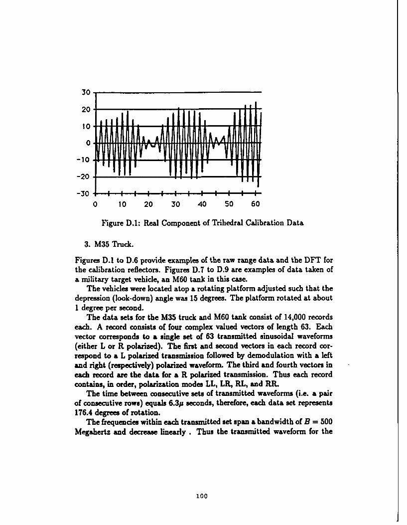
30-

210' --- -20

-30

0 10 20 30 40 50 60

Figure D.I: Real Component of Trihedral Calibration Data

3. M35 Truck.

Figures D.1 to D.6 provide examples of the raw range data and the DFT forthe calibration reflectors. Figures D.7 to D.9 are examples of data taken ofa military target vehicle, an M60 tank in this case.

The vehicles were located atop a rotating platform adjusted such that thedepression (look-down) angle was 15 degrees. The platform rotated at about1 degree per second.

The data sets for the M35 truck and M60 tank consist of 14,000 recordseach. A record consists of four complex valued vectors of length 63. Eachvector corresponds to a single set of 63 transmitted sinusoidal waveforms(either L or R polarized). The first and second vectors in each record cor-respond to a L polarized transmission followed by demodulation with a leftand right (respectively) polarized waveform. The third and fourth vectors ineach record are the data for a R polarized transmission. Thus each recordcontains, in order, polarization modes LL, LR, RL, and RR.

The time between consecutive sets of transmitted waveforms (i.e. a pairof consecutive rows) equals 6.3p seconds, therefore, each data set represents176.4 degrees of rotation.

The frequencies within each transmitted set span a bandwidth of B = 500Megahertz and decrease linearly. Thus the transmitted waveform for the

100

30

20

-10 1 VV

-20

-30 I I I I I I0 10 20 30 40 50 60

Figure D.2: Imaginary Component of Trihedral Calibration Data

1200

1000-

800

600.

400

200 t*~rt* c JFTrfrn nt i

0 10 20 30 40 50 60

Figure D.3: Modulus of DFT of Trihedral Calibration Data

101

30

20

0

-10

-20 -- -- -=- - _ -

-30 --

0 10 20 30 40 50 60

Figure D.4: Real Component of Dihedral Calibration Data

30-

20 - __-----

10'

0 ,

-10 I - -

-20' - -

-30' - 4--I I----+ 4I-+

0 10 20 30 40 50 60

Figure D.5: Imaginary Component of Dihedral Calibration Data

102

U 1200

1000-

800.

600.

400-

1 200.

I0 10 20 30 40 50 60

3 Figure D.6: Modulus of DFT of Dihedral Calibration Data

II*10

A A ,

I 0-

I -10

-20' M i i i i I Ii I I I10 10 20 30 40 50 60

Figure D.7: Real Component of M60 Tank Data (near -20*)

3 103

II

1 20

j 1011 0o

1 - 10V

-20 : : I , I I i0 10 20 30 40 50 60

Figure D.8: Imaginary Component of M60 Tank Data (near -20 ° )

i 200-.

iI 100

0

i 0 10 20 30 40 50 60

Figure D.9: Modulus of DFT of M60 Tank Data (near -20 °)

104

k-th column within a given pair of rows equals sin(2rfV - (k - 62)B/63]t)where f, equals the reference frequency.

For both vehicles, the angle 0, measured from head-on (0 degrees) coun-terclockwise, as a function of record index k is given by

I (k) = ak + b. (D.12)

For the tank a = .0128 and b = -23.9, thus the angle ranges 2 from -24degrees to 156 degrees.

For the truck a = .0128 and b = -34.6, thus the angle ranges from -35I degrees to 145 degrees.

2The data was divided into -blocks" of 2000 records for cam of shipment on floppydisks. It was discovered late in the study that one %blowk of tank datat was corrupted.Theme data were simply skipped leaving 12,000 records of M60 dats.

105

I Appendix E

Baseline Target ExtentI Calculation MethodI

This section details the baseline method for extracting target extent from aI phase history data sequence zk.

1 1. compute the Discrete Fourier Transform (DFT) 4 of the complex radardata,

I 2. compute the squared modulus of the transform results [uk1 ',

3. establish a threshold T > 0,

4. compute an estimate of the noise floor. Since the data provided does nothave any "empty" range cells, the average power A calculated from the16 range cells furthest away from the target, was used as the estimateof the noise floor. This was the best estimate available since the truetarget position was know to be in the center of the array k. The first8 and the last 8 range resolution cells were used to estimate A,

5. compute the indices I, and '2 of the first and last entries of ik 12 thatj exceed T x A,

6. compute target extent as 2 - 1 + 1.

I

I 106

Bibliography

I [1] C. S. Burrus and T. W. Parks, (DFT/FFT) and Convolution Algo-rithms, John Wiley and Sons, New York, 1985.

I [2] I. Daubechies, "Orthonormal bases of compactly supported wavelets",Communications on Pure and Applied Mathematics 1988, Vol. 41, 909-996.

[3] T. H. Einstein, "Generation of high resolution radar range profiles andrange profile auto-correlation functions using stepped-frequency pulsetrains," Project Report TT-54, Massachusetts Institute of TechnologyLincoln Laboratory, 18 October 1984.

[4] S. G. Mallat, "A Theory for multiresolution signal decomposition: thewavelet representation", (IEEE) Transactions on Pattern Recognitionand Machine Intelligence, July 1989, Vol. 11, no. 7, 674-693.

[5] H. L. Resnikoff and C. S. Burrus, "Relationships between the fouriertransform and the wavelet transform", Aware, Inc., AD900609, 1990.

[6] M. I. Skolnik, Radar Handbook, Second Ed., McGraw-Hill, New York,1990.

II

II

I 107