applications of geometric tolerancing to machine design

1

Applications of Geometric Tolerancing

to Machine Design

Second Edition

Faryar Etesami

Portland State University

Design for Fit

Applications of Geometric Tolerancing to Machine Design

Second Edition

Faryar Etesami Mechanical and Materials Engineering Department

Portland State University

ISBN 978-0-9914638-0-0

Copyright © 2016 by Faryar Etesami

All rights reserved. No part of this book may be reproduced or transmitted electronically

or otherwise without permission in writing from the publisher.

The information presented in this book and any associated software is included for

educational purposes only. The author and publisher make no warrantees of any kind

with regard to applicability or validity of the materials presented in this book.

Send Correspondence to: [email protected]

Preface

This book is written for students enrolled in an undergraduate program in mechanical

engineering (BSME) or similar programs. The material presented is based on my notes

for teaching mechanical tolerancing for nearly thirty years. The book’s emphasis is on fit

and alignment requirements for machine components. Fit assurance makes up the

majority of challenging applications in tolerancing. Design for specific functions is easy

by comparison. For design engineers, knowing how to apply geometric tolerances has

been a challenge even for engineers who have practiced geometric tolerancing for a long

time. The syntax and meaning of geometric tolerancing statements can be learned easily

and quickly but knowing how to use them correctly is much more difficult. For years I

taught the geometric tolerancing standards in great detail as one may teach a foreign

language using a dictionary. That method of training was fine for those on inspection or

manufacturing career paths but was not very useful to design engineers. Finally, I

decided to teach the subject not as a geometric tolerancing class but as a design-for-fit

class. I found this new method to be far more effective and useful to design engineers

than covering every detail of the GDT standard.

The objective of this book is to present the subject of design-for-fit in a format that is

suitable as a college-level course. I believe students learn in the context of simple

examples free of distractions. They are then able to apply what they learned in more

complex applications. For that reason, I have done my best to convey the concepts of

design for fit in the context of simple examples. Graduating mechanical engineers who

design and document parts and assemblies should have a basic understanding of the

design-for-fit principles presented in Chapters 1-9. The book can be used to support

a junior-level or senior-level class in a BSME program or it can make a companion

textbook for capstone design classes. Interested students or practitioners can follow up

with the more advanced topics in Chapter-10 and Chapter-11 on multipart fits and fit

analysis. Since this book does not cover every detail of the geometric tolerancing

standard I recommend having a copy of the standard document as an official and legal

reference. Low-cost pdf versions of the GDT standard can be found online.

Faryar Etesami

January 2016

1

CONTENTS

Chapter-1 Dimensions and Tolerances ....................................................... 5

1.1. Overview ...................................................................................................................................... 5

1.2. Evolution of tolerancing .............................................................................................................. 6

1.3. Geometric versus dimensional tolerances ................................................................................. 10

1.4. Importance of clear geometry communication practices .......................................................... 15

1.5. Functional feature vocabulary ................................................................................................... 16

1.6. Preferred practices in dimensioning .......................................................................................... 20

1.7. Figures of accuracy for dimensions and tolerances ................................................................... 38

Chapter-2 A Design Engineer’s Overview of Tolerance Statements - Part-I .................................................. 44

2.1. Overview ................................................................................................................................... 44

2.2. Interpretation of geometric tolerances ................................................................................... 44

2.3. Dimensional tolerances ............................................................................................................ 46

2.4. Geometric tolerances ................................................................................................................ 47

2.5. Tolerances of form .................................................................................................................... 50

2.6. Flatness ..................................................................................................................................... 50

2.7. Meaning of m symbol next to the tolerance value ................................................................. 53

2.8. Straightness .............................................................................................................................. 55

2.9. Circularity ................................................................................................................................. 56

2.10. Cylindricity ................................................................................................................................ 58

2.11. Tolerances of orientation ......................................................................................................... 59

2.12. Parallelism ................................................................................................................................ 61

2.13. Identifying the axis of an imperfect cylinder ........................................................................... 62

2.14. Perpendicularity ....................................................................................................................... 67

2.15. Angularity ................................................................................................................................. 70

2

Chapter-3 A Design Engineer’s Overview of

Tolerance Statements - Part-II ................................................. 77

3.1. Overview ................................................................................................................................... 77

3.2. Tolerances of location .............................................................................................................. 77

3.3. Position tolerance ..................................................................................................................... 77

3.4. Meaning of mmodifier applied to datum features ................................................................. 91

3.5. Composite position tolerance – multiple segments ................................................................. 93

3.6. Composite position tolerance – single segment ....................................................................... 96

3.7. Runout tolerances ..................................................................................................................... 98

3.8. Profile tolerances .................................................................................................................... 107

3.9. Profile tolerances in place of ± tolerances ............................................................................. 112

Chapter-4 Default Tolerances ................................................................. 128

4.1. Overview .................................................................................................................................. 128

4.2. Default tolerancing methods .................................................................................................. 128

4.3. Datum targets ......................................................................................................................... 133

4.4. Default tolerancing and small features ................................................................................. 137

4.5. Default tolerances for fillets and rounds................................................................................ 138

4.6. A different way of dealing with small features ...................................................................... 139

Chapter-5 Tolerance Design for Unconstrained Fits Between Two Parts

Part-I ..................................................................................... 150

5.1. Overview .................................................................................................................................. 150

5.2. Unconstrained fits versus constrained fits ............................................................................... 150

5.3. Fit assurance between two parts ............................................................................................ 154

5.4. Theoretical gages for tolerance statements that use the m symbol ...................................... 160

5.5. Fit formula ............................................................................................................................... 161

5.6. Default form control implied by limits of size .......................................................................... 164

5.7. Use of zero geometric tolerance at MMC ................................................................................ 165

5.8. Fit formula when using zero geometric tolerancing at MMC .................................................. 167

5.9. Defining a fit boundary without the m modifier ..................................................................... 167

5.10. A note on the use of modifiers ................................................................................................. 168

3

5.11. Unconstrained fits and Rule#1 ................................................................................................ 169

5.12. Unconstrained interference fits ............................................................................................... 171

Chapter-6 Tolerance Design for Unconstrained Fits Between Two Parts

Part-II .................................................................................... 176

6.1. Overview ................................................................................................................................. 176

6.2. An overview of the limits and fits standard (ANSI B4.2) ....................................................... 178

6.3. Preferred sizes ........................................................................................................................ 180

6.4. Offsets letters (fundamental deviations indicator letters) .................................................... 181

6.5. International tolerance grades .............................................................................................. 183

6.6. Preferred fits ........................................................................................................................... 183

6.7. Dependency of offsets and tolerance grades on basic size .................................................... 194

6.8. Tolerance design examples in precision fit applications ....................................................... 194

Chapter-7 Tolerance Design for Orientation-constrained Fits

Between Two Parts ................................................................ 208

7.1. Overview ................................................................................................................................. 208

7.2. The fit boundary and the theoretical gage ............................................................................ 210

7.3. A word on inspection .............................................................................................................. 216

7.4. MMC boundary as fit boundary .............................................................................................. 217

7.5. Situations where MMC modified tolerances cannot be used ................................................. 219

7.6. Datum feature flatness ........................................................................................................... 220

7.7. Is it necessary to specify axis straightness? ........................................................................... 225

7.8. Defining a fit boundary without the m modifier ................................................................... 227

Chapter-8 Tolerance Design for Location-constrained Fits

Between Two Parts ................................................................ 230

8.1. Overview .................................................................................................................................. 230

8.2. The fit boundary and the theoretical gage .............................................................................. 231

8.3. Datum priority ......................................................................................................................... 236

8.4. Datum frame precision ............................................................................................................ 241

8.5. Imperfect geometry relationships are not intuitive ................................................................. 243

4

8.6. Fit of feature patterns ............................................................................................................. 245

8.7. Simultaneous fit of different features ...................................................................................... 248

8.8. Additional alignment fit features ............................................................................................ 252

8.9. Situations where the use of m is not possible or recommended ............................................ 255

8.10. Defining a fit boundary without the mmodifier ..................................................................... 256

Chapter-9 Assemblies with Threaded Fasteners ...................................... 267

9.1. Overview ................................................................................................................................. 267

9.2. Fits using threaded studs or screws ....................................................................................... 267

9.3. Fits using threaded press-fit studs ......................................................................................... 269

9.4. Assembly with cap screws and threaded holes ...................................................................... 271

9.5. Assembly of two plates with loose bolts and nuts .................................................................. 272

9.6. Fastener applications - Example-1......................................................................................... 274




9.10. Tolerance design of press-fit inserts ...................................................................................... 287

Chapter-10 Tolerance Design of Multipart Fits .......................................... 295

10.1. Overview ................................................................................................................................. 295

10.2. Application of profile tolerances ............................................................................................ 296

10.3. Fits involving features-of-size ................................................................................................ 301

Chapter-11 Tolerance Analysis of Multipart Fits ....................................... 338

11.1. Overview ................................................................................................................................. 338

11.2. Tolerance analysis overview .................................................................................................. 338

11.3. Examples ................................................................................................................................. 339

5

Chapter-1 Dimensions and Tolerances

1.1. Overview

This chapter presents an introduction to tolerancing practice and suggests guidelines for

clear graphics communication. After a part’s exact geometry is defined in a CAD system

a design engineer must also specify the part’s geometric tolerances. Tolerances define

allowable deviations of part features from their theoretical definitions. Since

manufacturing variations are inevitable, tolerancing information allows production

personnel to select suitable processes and methods to meet part precision requirements at

minimum cost.

Tolerancing specifications include tolerance types and tolerance values. For example, if a

surface is to be flat with high precision, then the designer applies a standard flatness

tolerance symbol and specifies a tolerance value. The smaller the tolerance value, the

more flat the surface would be manufactured, but usually at a higher cost. The geometric

tolerancing standard to which the material in this book refers to is the ASME Y14.5-2009

standard, which from now on, will be referred to as the GDT standard. The GDT standard

provides a variety of symbols a designer can use to control various geometric aspects of a

part.

The design engineer’s challenge is to create a set of precision specifications that is just

enough to assure proper fit and function of a part in an assembly. The ability to create

well-toleranced parts is an important skill for a mechanical design engineer. Improper

use of tolerance types or tolerance values can affect the cost of production as well as the

fit and function of assemblies. To be safe, many designers resort to over-specification of

tolerances. Tolerance types that are not needed or tolerance values that call for

unnecessary precision would lead to higher production costs and delays in a variety of

ways such as:

The need for more expensive processes or machines

The need for additional or more time-consuming processing steps

Lack of in-house capability

The need for more expensive tooling

A reduction in throughput

The need for more expensive inspection tools

An increase in rework and reject rates

Excessive lead-times

On the other hand, lack of necessary tolerance types or tolerance values that do not call

for enough precision reduce the cost of production at the risk of non-assembly or

functional compromises. Some of the more common failures associated with lack of

sufficient geometric precision are:

Risk of parts not fitting properly into an assembly

6

Improper performance

Improper sealing

Loss of operation accuracy

Loss of power

Loss of functionally critical alignments

Improper thermal or electrical conduction

Structural Failures

Improper load distribution

Unexpected dynamic loads

Unexpected loading modes

Unacceptable changes of stiffness

Reduced service life

Excessive friction or wear

Excessive noise

Excessive heat

Excessive vibration

The great majority of tolerancing needs for typical parts relate to their fit requirements or

their alignment requirements necessary for fit. For that reason, this book primarily

discusses tolerancing needs for proper fit.

Like other engineering specifications, good tolerancing is not merely about what works

but what works at minimum cost. Geometric tolerances have a significant impact on the

final production costs.

1.2. Evolution of tolerancing

Before the industrial revolution, craftsmen often made the necessary parts of an assembly

and fit them together in their shops. Each part was custom made to fit where it needed to

fit. It was neither necessary nor wise to make all of the parts first and hope they would fit

together properly at the end. The practice of build-and-fit was possible because the entire

assembly was made by the same skilled worker in the same shop. Customers simply

expected the entire assembly to work as described with some desired overall dimensions.

Even today prototypes are often made this way because this method requires less

precision work than building all of the parts first and fitting them together later. It is also

easier and quicker for the design engineers to leave all the details to the manufacturing

personnel as long as the assembly works at the end.

Mass production made the build-and-fit scheme impractical. Parts needed to be made on

different machines and task specialization allowed high throughputs. Other skilled

workers or machines put the parts together forming the final assemblies. The necessity of

faster product introduction also resulted in specialization of skills. Shape design became

the responsibility of the designers, draftsmen assisted designers by creating detailed

drawings, production specialists designed the tooling and produced parts most efficiently,

and quality control specialists checked the accuracy of the parts. Drafting guidelines

7

were introduced to standardize the graphical communication of geometric information

between designers, manufacturing, and quality control people.

To make sure that the parts were made with sufficient accuracy to fit together during

assembly, design engineers had functional gages built and sent with their drawings that

described the part dimensions. Each functional feature of a part was to be checked with

two types of physical gages, a GO gage and a NOT GO gage. A part that would fit the

GO gage was assured to fit a mating part in the assembly. The GO gage, sometimes

made of wood, simply represented the worst-case geometry of a mating part for fit

purposes. Figure 1-1 shows a portion of a chainsaw assembly.

Figure 1-1. A portion of a chainsaw assembly

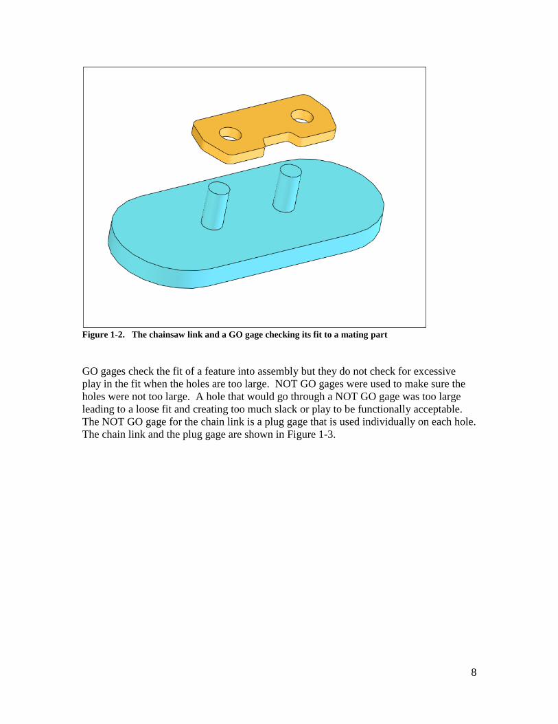
Figure 1-2 shows a chainsaw link with its two critical holes along with a GO gage which

is a flat plate with two pins. GO gages simulate the contacting surfaces and fitting

features of a mating part.

8

Figure 1-2. The chainsaw link and a GO gage checking its fit to a mating part

GO gages check the fit of a feature into assembly but they do not check for excessive

play in the fit when the holes are too large. NOT GO gages were used to make sure the

holes were not too large. A hole that would go through a NOT GO gage was too large

leading to a loose fit and creating too much slack or play to be functionally acceptable.

The NOT GO gage for the chain link is a plug gage that is used individually on each hole.

The chain link and the plug gage are shown in Figure 1-3.

9

Figure 1-3. A NOT GO plug gage for checking the size of each hole in the chainsaw link

An acceptable part feature would clear the GO gage, assuring fit, but not the NOT GO

gage, assuring acceptable play and proper function. Other non-critical features of parts

were assumed to be acceptable as made when the tools and workmanship conformed to

established standards of good manufacturing. No gages were made for non-critical

features.

Building and sending physical gages with part drawings were difficult to do in a design

environment. In later years, design engineers simply created separate drawings necessary

to build the gages at the manufacturing site with some added precision instructions. The

precision instructions, or tolerancing instructions, were in the form of ± variation limits

on the dimensions of the gages to be made. With this additional description of accuracy,

the gages could be built at the manufacturing site where the parts were being made.

Eventually, these ± limits were directly applied to the part dimensions from which

appropriate gages could be made to verify the fit and function of precision features. This

eliminated the need for the designers to create multiple sets of drawings, one for the part

and others for the gages. It also became easy to simply check the dimensions of the part

for conformance. Unfortunately, this practice led to serious unintended consequences.

Applying dimension limits by designers and checking dimensions by inspectors became

the norm in tolerancing until it was replaced by geometric tolerancing practices that once

again introduced the concepts of functional gaging back into the tolerancing standards

and tolerancing practice.

10

1.3. Geometric versus dimensional tolerances

At the time of its introduction, the geometric variation control based on ± limits on part

dimensions and angles were logical extensions of dimensioning, easy to apply, easy to

understand, and easy to verify. However, the ease of dealing with dimension limits is

true only when the geometry of the part remains free of deformations and distortions.

Deformations and distortions make it difficult to interpret the meaning of dimension

limits without subjectivity. As more knowledge was gained regarding the geometric

requirements of fit and function, it became clear that dimensional tolerances alone did not

provide the best specification toolbox for assuring fit and function.

The concept of gaging and gage description is at the heart of what constitutes geometric

tolerancing. A simple example can highlight the advantage of geometric tolerancing

over just using dimension limits. Consider rolling a heavy, tall refrigerator on casters

past a doorway. The width of the refrigerator is just below 835 mm and the width of the

doorway is just over 835 mm. There is a good chance, however, that the refrigerator

would not fit through. Figure 1-4 highlights the point.

Figure 1-4. The width of the refrigerator alone may not be sufficient to assure fit

On the left figure, the refrigerator and the doorway are shown to be free from all

distortions. In reality, however, this never happens. On the right figure the refrigerator is

tilted slightly to the left with respect to the plane of casters, while the doorway is

assumed to be free of distortions. The resulting arrangement leads to interference.

11

You can imagine how specifying the “width” dimension limits alone can put fit ability in

jeopardy. The homeowner who wants to assure fit using dimension limits must also

specify or explain to measure the width correctly as shown in Figure 1-5.

840

830

834

Figure 1-5. The width of the refrigerator must be measured in a way that is meaningful for fit

Of the three methods of measurement shown, only the 840 mm value is functionally

correct for fit. The other two measurements, albeit both reasonable measurements of the

“width” of the refrigerator, lead to incorrect values for fit. A tolerancing scheme based

on dimension limits simply ignores the reality that parts can have deformations and

distortions. You may describe the required method of measurement by notes but the

GDT standard provides an elegant way of describing exactly such a fit requirement using

a compact symbolic notation.

By making gages, the dimensional measurement confusion would never happen. The

gage for the refrigerator would be a perfect 835 mm doorway as high as the refrigerator

and made nearly perfectly with gage-making tolerances. If the refrigerator passes

through this gage properly, it would also pass though the real doorway. Note that the

gage geometry description by itself is not sufficient to assure a correct fit. The gaging

instructions are necessary to ensure the refrigerator passes through the gage while casters

are in contact with the floor. The GDT standard provides a set of symbols to easily

describe the gages and the gaging methods for common fit applications in assemblies.

The strength of the GDT standard specifications is that it allows a designer to specify the

12

precision needs of a part by following and mimicking the way the part is intended to fit

into an assembly.

Unlike dimensional tolerances, geometric tolerancing statements do not ask for any

numerical measurements at all. They simply describe the geometry of the necessary

gages to assure fit and function. Of course an inspector who does not want to build a

gage, for cost or practical reasons, is forced to make the necessary measurements to be

able to judge with confidence whether the feature would pass such a gage if it had been

made. In the case of the refrigerator, the inspector may easily measure the width of 830

mm and also measure the angle of tilt. Combing the two measurements would come

close to the functional dimension of the refrigerator.

In design, the basic elements of function are features. Features are collections of

surfaces that, as a whole, can be associated with a particular function. This is similar to

the use of language in which the basic elements of communication are words not

individual letters. A feature-based geometric specification language directly deals with

features and their functions. The geometric tolerancing standard provides this feature-

based language and a gage-based methodology for geometry control. Geometric

tolerancing allows the design engineers to separately control various geometry aspects of

features when needed. Such aspects include feature size, form, orientation, and location.

Today, the preferred method of specifying acceptable manufacturing tolerances is a

combination of geometric and dimensional tolerances. Dimensional tolerances are

mainly used to describe size limits of cylindrical features or width features (slots and

rails). Figure 1-6, for example, shows both the dimensional and the geometric

tolerancing methods of controlling the size and the distance between two holes. The

geometric method will be explained later in detail.

13

Figure 1-6. Specifying the tolerance on the distance between two holes using dimensional

tolerancing (top) and geometric tolerancing methods (bottom)

The two schemes both control the size and distance between the two holes but they do not

have the same meaning. The specification shown in the bottom figure is functionally

more meaningful and preferred to the method shown on the top figure. The details will

be presented in later chapters.

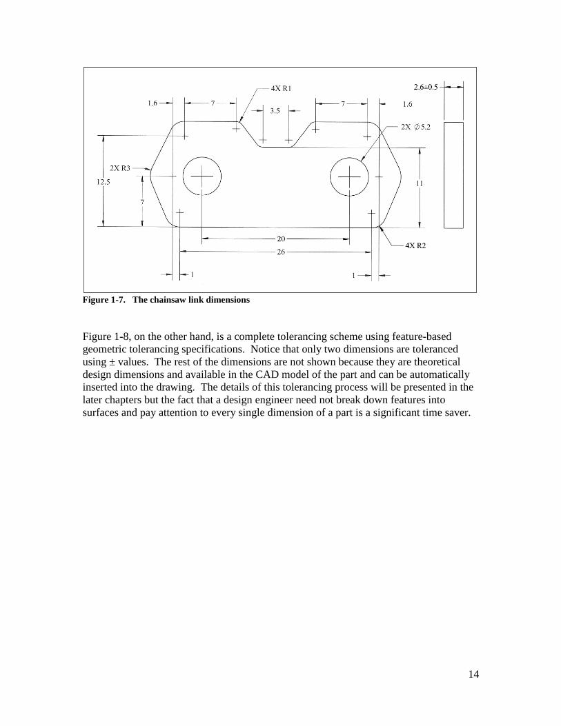
Figure 1-7 shows the dimensions necessary to define the geometry of the chainsaw link

previously discussed. In a tolerancing scheme based on ± limits on dimensions, each

dimension needs to have an associated tolerance either explicitly or implicitly through

default tolerances in order to create a production drawing. The chainsaw link requires a

lot of ± tolerances to be fully toleranced. Except for the plate thickness tolerance, these

tolerances are not shown on this figure because the drawing becomes difficult to read.

14

Figure 1-7. The chainsaw link dimensions

Figure 1-8, on the other hand, is a complete tolerancing scheme using feature-based

geometric tolerancing specifications. Notice that only two dimensions are toleranced

using ± values. The rest of the dimensions are not shown because they are theoretical

design dimensions and available in the CAD model of the part and can be automatically

inserted into the drawing. The details of this tolerancing process will be presented in the

later chapters but the fact that a design engineer need not break down features into

surfaces and pay attention to every single dimension of a part is a significant time saver.

15

Figure 1-8. The chainsaw link fully toleranced with geometric tolerances

Geometric tolerancing promotes a feature-based and functional approach to tolerancing

and allows a design engineer to control feature size, form, orientation, and location with

varying degrees of precision as needed for fit and function. For example, in a feature-

based way of thinking about tolerances, the chainsaw link has only three functional

features. The first feature is the entire outer profile and is controlled with a single

tolerance statement with low precision. The second feature is the pattern of two holes

controlled by another geometric tolerance statement at high precision. The third feature

is the plate thickness controlled by a dimensional tolerance at medium precision.

1.4. Importance of clear geometry communication practices

Design engineers communicate the theoretical shape of parts to manufacturing through

dimensioning. While the complete geometry of a part can be accessed through its 3D

CAD model without effort, the use of 2D drawings is still quite common for geometry

communication. It is perfectly fine for production to only create the tolerance

requirements of a part along with the CAD model describing the theoretical geometry of

a part. Note that a paper drawing is a legal document that can be used to settle quality

disputes. The rest of this chapter is mainly for readers who need to be able to create

high-quality 2D drawings. CAD systems can also create 2D drawings automatically from

the parameters and dimensions entered during modeling. If care is exercised to model the

16

part using the dimensions that are intended to be on the final drawing, then little work

remains after the CAD system generates the 2D drawings automatically.

Poorly dimensioned parts can lead to incorrect geometry interpretations or delays due to

the need to clarify vague or missing information. Part drawings are not just to

communicate information to manufacturing as design engineers often discuss the merits

of different design alternatives using 2D dimensioned drawings as well. Poorly

dimensioned parts reduce the effectiveness of design work as well. Today, the old

engineering graphics courses are quickly disappearing as a part of the mechanical

engineering curricula, replaced by 3D solid modeling classes. The lack of basic graphics

training has led to new design engineer’s inability to create well-dimensioned parts.

Improper dimensioning often leads to frequent conflicts with manufacturing personnel.

A well-dimensioned part drawing is like a well-written report. Good writing is about

conforming to good writing principles that give a reader easy access to the information

presented in a report. Likewise, a well-dimensioned part drawing presents the geometry

of every part feature in a format that is easy to understand completely and quickly. As a

badly written report is often an indication of poorly-understood ideas, a badly

dimensioned part drawing is often a sign of poorly-understood fit and function needs.

To avoid unnecessary communication problems with manufacturing and others, design

engineers should learn the simple rules of good dimensioning practice and develop the

habit of delivering high-quality drawings to manufacturing and other design engineers.

At first, conforming to good dimensioning rules may appear burdensome but with

practice the methods become natural, intuitive, and easy to follow. The ability to

conform to good dimensioning practices is also helpful in adhering to good tolerancing

practices.

A lazy approach to dimensioning is to take a part drawing and randomly add dimensions

to it until it is fully defined. This approach often leads to under-defined or over-defined

parts with information scattered without any logic or organization. This method conveys

little understanding of fit and function needs. A better approach to dimensioning is to

recognize that each part is made up of a collection of features. Each feature (or feature

pattern) can be described by a set of dimensions that define the shape of the feature itself

and a set of dimensions that locate the feature with respect to other part features. In this

respect, the word “feature” refers to a collection of part surfaces with a particular

function. The function need not be precision as long as the feature has a particular

purpose.

1.5. Functional feature vocabulary

It is helpful to use the proper feature vocabulary when dimensioning or communicating

geometry information to other engineers. Figure 1-9 shows the typical features of a shaft

in power transmission applications. Using a functional feature vocabulary helps thinking

in terms of features and not just individual surfaces.

17

Figure 1-9. A transmission shaft with its associated functional features

Grooves and holes are often used with other identifiers such as snap-ring grooves or

spring pin holes. Common features associated with fasteners are shown in Figure 1-10.

Figure 1-10. Various kinds of fastener-related features

18

Figure 1-11 shows some other common features on plate-like parts. A boss is a short

raised surface of any shape. A profile is any combination of surfaces grouped together

for functional and tolerancing purposes. Profiles can be internal (pockets) or external.

Figure 1-11. Other common features of plate-like parts

Figure 1-12 shows some of the common features of parts that usually fit onto rotating

shafts.

19

Figure 1-12. Common features of parts used with rotating shafts

The hub is the bulky part in the center of a wheel or a gear. The flange is the relatively

thin disk attached to a hub. A D-hole is a hole with a flat face that fits into a D-shaped

shaft for torque transmission. A lip is a small recess that fits a mating hole to create a fit

with minimal play.

Figure 1-13 shows a shaft with several geometric features in addition to the main

cylindrical shapes. A good approach to dimensioning this part is to recognize its

functional features and completely dimension each feature’s internal geometry and

location until no features remain. Thinking like manufacturing, a feature that is fully

dimensioned is like a feature that is fully made. It is a good practice to check every

feature of a part to make sure they are properly defined before sending the drawing to

manufacturing. It is also a good practice to change your role and see the part as a virtual

machinist who is going to make the part you designed. When dimensioning the part

features, complete a feature’s dimensioning before going to the next one.

20

Figure 1-13. A transmission shaft with its associated functional features

A neck is a groove between two different shaft diameters. The drawing and

dimensioning for this part will be presented later in this chapter. The next section

presents the necessary guidelines to create well-dimensioned parts.

1.6. Preferred practices in dimensioning

Most of the rules of dimensioning are developed to communicate complete geometry

information clearly with minimal clutter. It is emphasized again that a drawing should

not be viewed as a collection of lines and curves but as a collection of features. Once

every feature is properly dimensioned, the dimensioning task is complete. The drawing

reader should not only find all the necessary information to construct each feature of the

part but find them easily and quickly where he/she expects them to be placed. If you

have had no drafting training I suggest that you visit some web sites where more drafting

rules and examples are presented.

In order to reduce the number of needed dimensions, the following geometric

relationships are true in a part drawing. When no information is provided to indicate

otherwise, the following relationships are implied:

Lines that appear to be perpendicular are perpendicular.

Lines that appear to be parallel are parallel.

Lines that appear to be collinear are collinear.

Lines and curves that appear to be tangent are tangent.

Cylindrical features that appear to be coaxial are coaxial.

21

Lines mentioned in the above rules also include the centerlines connecting the features of

a pattern, such as a pattern of holes, whether such connecting lines are shown or not. The

following geometric relationships are not implied when left unspecified.

Lines that appear to have equal lengths are not implied to have equal lengths.

Diameters and radii that appear to be equal are not implied to be equal.

Features that appear to be symmetrically located with respect to a center plane or

axis are not implied to be symmetrically located unless other information is

provided.

Figure 1-14 illustrates some of the above rules. The dimensioning of this and other

example parts shown in this section may not be complete to better illustrate certain key

points.

Figure 1-14. Avoid double dimensioning. Lines that appear collinear are collinear

The crossed out dimensions represent repeated dimensioning and should be removed.

The 30 mm dimensions are both necessary as the appearance of equal length lines does

not imply equal length lines. Similarly, the hole feature appearing in the middle of the

part does not imply that it is in the middle and must be located both horizontally and

vertically. If the 80 mm dimension is not shown, as in Figure 1-15, then the center plane

of another feature should be shown to imply that the hole axis is aligned with the center

plane of another feature. A geometric tolerance statement would also be necessary to

22

identify which feature the hole is aligned with as multiple features may qualify. The

procedure for applying such tolerances will be presented in later chapters. It is worth

noting that centering or alignment implies a dimension of zero which is not shown on a

drawing. Therefore, in strictly dimensional +/- tolerancing, there is no ability to indicate

how precisely the features are to be centered or aligned. Fortunately, that is not a

problem in geometric tolerancing. The side view also shows that the 40-mm slot is to be

centered to the 60-mm outer rail feature. A tolerance statement is necessary to show the

level of centering precision. If in the side view a dimension of 10 mm is shown then the

center plane lines should be removed.

Figure 1-15. Extended centerlines should be drawn to indicate that a feature is centered with

respect to another feature

A smaller scale 3D view is often added to a drawing but the drawing interpretation must

not rely on such 3D images. Three dimensional models can be dimensioned but the

practice is not uniform or widespread. In this book dimensions are not shown on 3D

models or assembly drawings. This book uses the 3rd angle projection format which is

commonly used in the United States.

Views that are not needed should be removed. You may insert additional views that you

feel would be needed to correctly interpret the drawing or to provide additional

dimensions. However, adding unnecessary views and dimensions may reduce the

readability of a drawing.

When creating drawings you are expected to adhere to other rules and preferences listed

below. Not following these rules usually reduces the efficiency of graphical

communication. However, there are always cases where deviation from stated

preferences may be justified. The most important rule is to provide a complete and clear

description of part geometry.

23

General Rules and Preferences

1. In the Unites States the American National Standards Institute (ANSI) drafting

display format is preferred. This standard formatting controls all the display details

such as the display of dimension text sizes, notes, line thicknesses, line formats, and

symbol sizes. All dimension text and notes are to be horizontal. The CAD system

will do this automatically when ANSI format is selected.

2. Draw and dimension the entire part. The use of the symmetry symbol to reduce the

number of required dimensions is not a preferred practice.

3. Select a front view that best shows most of the important features of the part. When

necessary, other views (top, bottom, right, left, and rear) are to be placed around the

front view. The views must align and have the same scale.

4. Decimal millimeter values are used for dimensions in this book. When a value is less

than one millimeter, a zero is to be shown before the decimal point. Trailing zeroes,

however, are to be avoided.

5. Avoid odd dimensions or unusual precision unless well-justified. Most part

dimensions can be adjusted slightly to make them more rounded. Using extra figures

of accuracy where they are not needed would make the part more costly to make. A

simple number rounding rule will be presented later in this chapter.

Figure 1-16 shows a part with three dimension specifications. Unusual and unnecessary

precision should be avoided and the trailing zeroes should not be shown.

Figure 1-16. Avoid unusual precision or trailing zeroes

24

Dimension and Extension Lines

6. Do not use an existing line as a dimension line. This includes part profile visible

lines, continuation of visible lines, hidden lines, centerlines, or extension lines. All

dimension lines must be separately drawn.

7. Place dimension values centered between the arrows when there is sufficient space

between the arrows.

8. Place dimension lines so they do not intersect.

9. Each dimension line must have its own end arrows. Arrows are not to be shared

between dimensions.

10. Avoid using part profiles as extension lines.

11. When extending centerlines to be used as extension lines, use the centerline line

format.

12. Minimize intersection between dimension lines and extension lines. Also minimize

intersecting extension lines.

13. Point leaders to lines at an angle other than 0 or 90 degrees (preferably closer to 45

degrees).

14. Leaders pointing to circular features are to be radial in direction.

Figure 1-17 shows examples of inappropriate placement of dimension values and use of

part profile lines as extension lines.

Figure 1-17. Place dimensions outside the part and do not use part boundary as extension lines. Do

not share arrows between two dimension lines

15. Occasionally the part profile can be used as extension lines when separate extension

lines become long and intersect many other lines creating confusion. A common

example is in shafts with many features as shown in Figure 1-18.

25

Figure 1-18. Using part profile as extension lines is preferred for shafts with several features

The dimensions, however, are best to be placed outside the part profile.

Dimension Placement

16. Place dimension text outside the part view boundary or at least outside the part outer

profile box. When space allows, place dimensions between views.

17. When dimension lines are too close, stagger dimension values so the text is easy to

read.

18. Align the dimension lines when possible. Note that each dimension must have its

own dimension line and its own arrows.

19. Maintain a uniform distance of about one character height between parallel dimension

lines. The closest line to the part profile is placed at a distance of about 1.5 character

height.

20. Keep the dimensions that define a feature close together and close to the feature and

preferably on the same view. The reader should easily locate all of the dimensions

related to a feature.

21. When it is necessary to put words on the drawings they should be all capital letters.

However, standard symbols have been developed to minimize the use of words – use

words only when there are no symbols to convey the message. For example, the

word THRU is commonly used to indicate clearance holes or cuts when section views

or hidden lines are not used to show the feature depth.

22. Favor feature-based dimensioning in which dimensions define size and location of

features. Identify the features, dimension their internal geometry, and then use

functional dimensions to locate the entire feature with respect to other features.

26

Repetition Symbol

23. Use the repetition symbol nX (such as 4X) for repeated features, preferably features

that form a clear pattern and are countable on the same view. Do not use other text

such as 4 PLCS or 4 HOLES, etc.

24. When features (referred to by nX) are not all visible on the same view, they should be

clearly identifiable on other views. Common features for which nX is used are

patterns of holes, bosses, slots, rails, fillets, and similar patterns.

25. Use nX when the referenced feature is clearly and uniquely identifiable, otherwise

use separate dimensions.

26. Every feature count of nX must refer to a separate feature. The fillet that appears on

the top and bottom of a shaft are the same feature and count as one.

Figure 1-19 shows a plate part with a pattern of four holes and a cross hole. Note that the

use of THRU for the 6.6 mm cross holes is not appropriate because it is not clear whether

the hole is through the first section of the plate or both. One may use THRU BOTH but

the hidden lines are preferred here to indicate the extent of the cross hole. Also, the

extended centerline on the side view indicates that the hole is centered relative to the

thickness of the plate. The pattern of four holes is internally defined by 60 mm and 14

mm dimensions and then the pattern is located with respect to the left edges using 30 mm

and 8 mm dimensions. The locating dimensions must be chosen to be functionally

important. In this case the pattern location with respect the left face and bottom face are

important.

Figure 1-19. Dimensioning of feature patterns

27

27. Place all the related dimensions of a feature close to the feature, close together, and

preferably on a single view. A person reading a drawing should mentally construct a

feature quickly with one look.

28. Specify the important functional dimensions first. Never alter the functional

dimensioning scheme of a part thinking that manufacturing prefers it in a different

way. Manufacturing people are well-trained to find the best way to create the needed

precision. Manufacturing method decisions depend on tolerances and not on

theoretical dimensions. On the other hand, designers that discuss possible

modifications of the design would like to see the most important and functional

dimensions on the drawing.

Figure 1-20 shows some of the other dimensions for the example part shown earlier.

When a dimension can be shown on two different views, select the view in which the

dimension is easier to interpret. For example, the lower step height of 20 mm is easier to

interpret on the front view than the side view.

Figure 1-20. Complete dimensioning of the part

As mentioned before, the appearance of centerlines in the side view indicates that the slot

feature is centered to the 60-mm thickness feature. Without the centerlines the part is not

clearly defined. To avoid the appearance of missing dimensions a reference dimension

can be applied when necessary. A reference dimension is a dimension in parenthesis.

For example, a reference dimension of (80) can be added to the hole to emphasize that

the hole location is defined by alignment.

29. You should avoid over-dimensioning or repeated dimensions for the same feature.

Over-dimensioning means specifying a dimension or angle that can be calculated

from the already specified dimensions and angles. In cases where it is not clear that

two features have the same dimension, repeated dimensions can be used for clarity.

Over-dimensioning, however, is not an error when used with geometric tolerances - it

just makes the drawing busier.

28

30. Minimize the use of TYP which stands for “typical” unless the referenced features are

obvious. A common application is for a part with a large number of fillets or rounds

on its edges such as in molded parts.

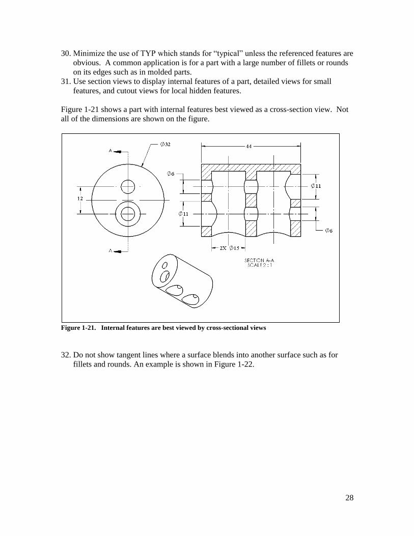
31. Use section views to display internal features of a part, detailed views for small

features, and cutout views for local hidden features.

Figure 1-21 shows a part with internal features best viewed as a cross-section view. Not

all of the dimensions are shown on the figure.

Figure 1-21. Internal features are best viewed by cross-sectional views

32. Do not show tangent lines where a surface blends into another surface such as for

fillets and rounds. An example is shown in Figure 1-22.

29

Figure 1-22. Do not show tangent lines

33. Use compact specification formats to efficiently dimension common features such as

counterbored holes, countersunk holes, blind holes, chamfers, keyways, etc. In a

compact format all of the feature dimensions are place in the same spot.

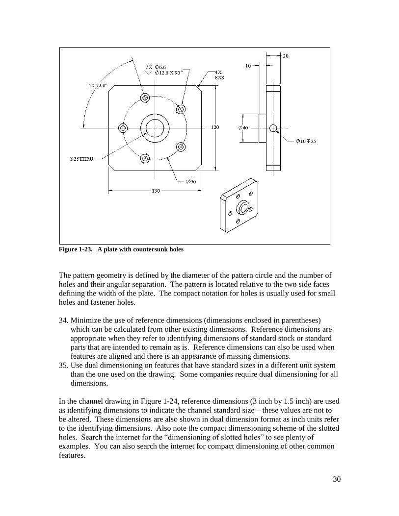
The part shown in Figure 1-23 is a plate with a pattern of five countersunk holes, four

chamfered edges, and a blind cross hole.

30

Figure 1-23. A plate with countersunk holes

The pattern geometry is defined by the diameter of the pattern circle and the number of

holes and their angular separation. The pattern is located relative to the two side faces

defining the width of the plate. The compact notation for holes is usually used for small

holes and fastener holes.

34. Minimize the use of reference dimensions (dimensions enclosed in parentheses)

which can be calculated from other existing dimensions. Reference dimensions are

appropriate when they refer to identifying dimensions of standard stock or standard

parts that are intended to remain as is. Reference dimensions can also be used when

features are aligned and there is an appearance of missing dimensions.

35. Use dual dimensioning on features that have standard sizes in a different unit system

than the one used on the drawing. Some companies require dual dimensioning for all

dimensions.

In the channel drawing in Figure 1-24, reference dimensions (3 inch by 1.5 inch) are used

as identifying dimensions to indicate the channel standard size – these values are not to

be altered. These dimensions are also shown in dual dimension format as inch units refer

to the identifying dimensions. Also note the compact dimensioning scheme of the slotted

holes. Search the internet for the “dimensioning of slotted holes” to see plenty of

examples. You can also search the internet for compact dimensioning of other common

features.

31

Figure 1-24. Use of reference dimension and dual dimensioning on a standard C-channel

36. When specifying threads, use the standard thread designations such as M6 x 1. Do

not separately dimension the diameter of such threaded features.

37. Do not use process information to convey geometry information. For example, do

not specify “USE 10-mm DRILL” in lieu of actual hole dimension limits. Also, do

not use specifications that refer to standard parts like “CUT FOR #205 WOODRUFF

KEY” as a substitute for specifying Woodruff keyway’s dimensions.

38. Show preference to dimensioning distances rather than angles. Angles are usually not

shown unless the angle is functionally important.

39. Place feature dimensions on the views where the feature shape information is best

seen. For example, when dimensioning the width of a slot feature, dimension the

view in which it is clear whether the feature is a slot or a rail. When dimensioning the

size of a cylindrical feature, place the dimensions on the view in which it is clear

whether the feature is a hole or a boss.

40. Do not use center marks for fillets or arcs when no dimensions are necessary to locate

their centers. Always show the center marks for cylindrical holes or bosses that fit

other features and show the axis of cylindrical features.

41. When a partial cylindrical feature is used as a fit feature (i.e. something fits into that

feature), use diameter dimension – otherwise use radius dimension.

Some of the points mentioned above are illustrated in Figure 1-25.

32

Figure 1-25. Dimension slot and rail features in views where their depth can be seen

Note that the slots and the rail are dimensioned in views where their depth can be seen.

The slot and rail depths, widths, and locations are shown close together. The holes are

dimensioned in the section view where the feature type, size, and depth can be seen

together. The geometry of the D-shaped boss is shown in the profile view where the D-

shape is best seen. The center feature is located to the bottom edge (75 mm) and to the

edge of the rail (40 mm).

Pattern Dimensioning

42. Use dimensions to fully describe the internal geometry of a pattern and then use

dimensions to locate the pattern with respect to other functionally relevant features.

43. Connecting the centerlines of holes in a pattern is preferred but they can be implied

and left out when the pattern lines reduce the readability of the drawing.

The part shown in Figure 1-26 has a pattern of four counterbored holes. The pattern is

170 mm by 55 mm and it is located with respect to the lower left corner edges. The

pattern connecting lines are not shown in this case. The shape of the slotted hole is

defined by its length (120 mm) and its width (15 mm) while its location is specified by its

distance to the left face (40 mm) and the lower face (40 mm).

33

Figure 1-26. A plate with a pattern of counterbored holes

You can think of a feature pattern as a solid piece like a piece of furniture such as a

dining table. When locating a piece of furniture we pick two edges and specify the

distance of these edges to the walls with two numbers. The rest of the dimensions are

defined by internal dimensions. Always use a minimum number of dimensions to locate

a pattern.

Hidden Lines

44. Do not show hidden lines unless they help show the extent of features not visible in

other views. When required, only show the hidden lines for the necessary features.

45. Do not dimension to hidden lines unless it is clear and simplifies the dimensioning or

when it reduces the number of views.

Additional Examples

Figure 1-27 shows the first dimensioning step for the shaft shown previously. The shaft

has a number of features associated with power transmission application. The first step

is to describe the shaft diameters, lengths, and functionally important shoulder-to-

shoulder distances.

34

Figure 1-27. Dimensioning of shaft diameters and shoulder-to-shoulder distances

After the dimensioning of the shaft diameters, including the left threaded diameter, the

other features need to be dimensioned. Each feature should be identified and completely

described before going to another feature. The first two selected features are:

The rectangular keyway on the right end of the shaft

The shaft neck close to the rectangular keyway

Figure 1-28 shows the necessary views to dimension the rectangular keyway and the

shaft neck. The width and depth of the keyway are described in the V-V section view

while the length is shown in the top view. The neck detail is shown in a detailed view for

clarity. To save space the detailed view and section view are not labeled.

35

Figure 1-28. Dimensioning of the rectangular keyway and the 2 mm wide neck

Note that the center plane of the keyway slot coincides with the axis of the shaft. This

means the two features are aligned. We can also show the 3 mm distance between the

edge of the slot and the center lines.

Two additional features of the shaft are:

The cross hole for a spring pin

The Woodruff keyway

Figure 1-29 shows two additional section views to dimension the cross hole and

Woodruff keyway. The Woodruff key is a standard key with a 28 mm diameter, 6 mm

thickness, and 11 mm height. The manufacturer calls for the width of the keyway to be 6

mm, the radius of the keyway to be 14 mm, and the depth of the keyway to be 7.5 mm

below the surface. The 7.5 mm depth leads to a distance of 32.5 mm between the keyway

bottom and the opposite face of the shaft. Search the internet for “dimensioning of

Woodruff keyways” for some examples.

The size of the spring pin hole is indicated to be 5.1 mm to match the manufacturer’s

recommendation for a 5 mm spring pin. The 20 mm functional location is specified on

the section view. Finally, the compact chamfer notation should be added to describe the

chamfer detail at the end of the shaft. The internal geometry of all the features is now

defined and each feature is adequately located.

36

Figure 1-29. Dimensioning of the spring pin hole and the Woodruff keyway

The part shown in Figure 1-30 is the drawing for a flange shape representing parts that

attach to a shaft and usually have hubs, keyways, bearing holes, centering bosses, and

fastener hole patterns. Flange-type parts are best shown using front and section views.

Note that the inner D-shaped cylindrical hole is dimensioned as a diameter because this

hole is intended to fit a shaft. Other cylindrical dimensions are shown in the section view

where it is clear whether they are bosses or holes.

37

Figure 1-30. A typical flange-type component that often fits shafts and bearings

Missing dimensions and vague geometry information are serious errors and must be

avoided. Always check for missing dimensions at the end by pretending to be a virtual

machinist attempting to build all of the part’s features using a virtual milling machine and

a virtual lathe. Going through this virtual building procedure catches missing or vague

information and also alerts you about features that may be difficult to make

economically. Subsequently the design may be altered for easier manufacturing.

Figure 1-31 shows the dimensioning method used to describe the geometry of the crank

part. While dimensioning to the points of tangency between lines and curves is not

preferred, in this case the 70 mm flat side distances are dimensioned to define the

theoretical shape of the part.

38

Figure 1-31. Dimensioning of a part with bent features

1.7. Figures of accuracy for dimensions and tolerances

When a theoretical dimension need not be controlled with precision, it is a good practice

and often most economical to round the dimension value up or down as much as possible

without being objectionable for other reasons. For example, if the theoretical model for a

holding bracket happens to have a precise dimension without a particular reason, consider

dropping the unnecessary figures of precision. For example, if a bracket dimension,

based on some strength calculations, comes out to be 247.652 mm, consider using 247,

250, or 240 mm instead. If the dimension is the result of some analysis other than those

associated with precision fits, apply the 1% dimension rule. Simply calculate 1% of the

dimension (in this case about 2.47 mm) and round the number up or down to within the

1% value. In this case, a rounded value can be any number between 245 and 250 mm.

If the theoretical dimension is a result of precision fit calculations, apply the 1% rule to

the tolerance value to get a more rounded value for the theoretical dimension. For

example, suppose the tolerance applied to a 247.652 mm size dimension is to be ± 0.8

mm. One percent of the tolerance is ± 0.008 mm. Add and subtract this 1% of the

tolerance value to the theoretical dimension to obtain a high and a low acceptable value.

39

In this case the high value is 247.660 and the low value is 247.644 mm. Use the

roundest number between these limits. In this case 247.65 mm is a good choice. The

resulting specification becomes 247.65 ± 0.8 mm.

Exercise Problems

1. Use a CAD system to model and fully dimension the housing endcap shown in Figure

1-32. The outer diameter of the part is 52 mm. The other dimensions are up to you.

Figure 1-32. The front and back views of the housing endcap

2. Use a CAD system to model and fully dimension the turning support shown in Figure

1-33. The overall width of the part is 80 mm. The other dimensions are up to you.

Figure 1-33. The turning support

40

3. Use a CAD system to model and fully dimension the part shown in Figure 1-34. The

shaft is 325 mm long. The 30 mm diameter cylinders fit to ball bearings. The

keyway in the middle supports a gear and the keyway at the end of the shaft supports

a belt pulley. There is a M8x1 threaded hole on one end of the shaft as shown in the

figure. The drill hole for the threaded hole is 19 mm deep and the thread is 16 mm

deep. The rest of the dimensions are up to you.

Figure 1-34. A power transmission shaft

4. Use a CAD system to model and fully dimension the part shown in Figure 1-35. The

plate length is 200 mm and the counterbored holes are for 6 mm screws.

41

Figure 1-35. A flange with counterbored holes

5. Use a CAD system to model and fully dimension the plate part shown in Figure 1-36.

The plate is purchased as 4 inch by 4 inch with a thickness of 0.125 inch. Display

these dimensions as reference and as dual dimensions. The corner holes are 5 mm.

The pattern of four holes in the middle are 4 mm threaded holes. The pattern of two

holes are 3 mm threaded holes. The center feature is a through hole.

42

Figure 1-36. A plate with threaded and through holes

6. Use a CAD system to model and fully dimension the plate part shown in Figure 1-37.

The plate is 1 inch wide and 0.25 inch thick. Display these dimensions as reference

and as dual dimensions. The pattern of two countersunk holes are for 3 mm screws.

The set screw hole is also for a 3 mm screw.

Figure 1-37. A plate with threaded holes and countersunk holes

43

7. Use a CAD system to model and fully dimension the square tubing shown in Figure

1-38. The square tubing is 2.5 inch by 2.5 inch in outer dimensions. The thickness is

0.25 inches. Show these dimensions as reference in dual dimension format. The

center holes are aligned but have different sizes. There is pattern of two threaded

holes and two clearance holes on each side face of the tubing. There is a pattern of

four clearance holes on the bottom surface. Create appropriate drawings for this part

and complete its dimensioning.

Figure 1-38. A square tubing with patterns of holes and a slot

8. Find a real machine part and measure its features. Then, use your CAD system to

model and fully dimension the part. Include an actual picture of the part.

9. Search the internet for recommended dimensioning methods of other common

features. Use your CAD system to model a simple part with a variety of common

features and fully dimension the part.

44


Tolerance Statements - Part-I

2.1. Overview

The next two chapters present a designer-oriented overview of the GDT standard

tolerance specification statements. The objective here is to provide a basic

understanding of how a designer can call for geometric accuracy and how geometric

tolerancing statements are interpreted. Geometric tolerances along with dimensional

tolerances (± or dimension limits) comprise the designer’s toolbox for controlling the

geometric aspects of part features needed to ensure fit and function. This chapter

presents the tolerances of form and orientation. The following chapter continues with

tolerances of location and profile.

2.2. Interpretation of geometric tolerances

The interpretation of most geometric tolerancing statements is straightforward and

intuitive. Each tolerance statement can be interpreted by creating a theoretical gage

which serves as an acceptance template. The gage dictates how close the features should

be to their perfect geometry in order to be acceptable. The gage be conceptually held

against the actual part to check the part’s acceptability. Not only is the gage geometry

important but the manner of holding the gage against the actual part can be important as

well. Tolerance control statements disclose the information necessary to build the

theoretical gages and define the method of gaging. Theoretical gages reflect the true

meaning of tolerance statements but they may not be practical to build or use. Inspection

personnel are trained to use alternative procedures and come up with decisions that

conform to those obtained by theoretical gaging.

As an example, Figure 2-1 shows a theoretical gage and the theoretical gaging procedure.

45

Figure 2-1. Theoretical gage (left) and theoretical gaging (right)

The left side of the figure shows a theoretical gage made up of two planes and a small

diameter cylinder that appears like a line. The right side of the figure shows the gaging

process in which the gage is aligned against the actual part. This chapter and the next

chapter present the details of how to define theoretical gages for each tolerance statement

and how to align them against actual parts.

Most theoretical gages are three-dimensional. They are created from planes and

cylinders and other 3D features. There are also tolerance statements that control feature

cross-sections. These tolerance statements lead to two-dimensional gages or planar

templates that are constructed on a plane.

When tolerance statements are applied to part surfaces or cross-sectional curves, the

tolerance verification is straightforward and simply requires checking the subject feature

surfaces or cross-sectional curves against a tolerance zone. When tolerance

specifications are applied to axes or center planes, the tolerance interpretation must

prescribe how the subject feature is to be derived from the surface features. The method

of identifying the derived features is a part of the gaging process.

Theoretical gages along with the gaging instructions capture the true meaning of the

tolerancing specifications. In describing a tolerance statement, designers only need to

explain the gage geometry and the gaging procedure. Theoretical gages are easy to

define as their geometry closely mimics the tolerance specification. Geometric tolerances

allow design engineers to control a feature’s size, form, orientation, and location with

respect to other features.

46

2.3. Dimensional tolerances

Dimensional tolerances refer to the direct dimension limits or ± tolerance values and can

be applied to any dimension that defines a part. When dimension limits are applied to

features known as features-of-size (FOS), the meaning of the dimension limits is

explained in the GDT standard in terms of acceptance gages. Regular FOS are

cylindrical, spherical, or width features (slots and rails) that are toleranced with

dimension limits. When dimension limits are used to control size or location of other

features, their meaning is not defined in terms of gages - they are defined in terms of

measured dimensions. This means the inspector has to make a measurement that

corresponds to the toleranced dimension and compare that against the limits. Since

manufactured features have deformations and distortions, it is impossible to assign a

unique measured value to such dimensions without subjectivity. For that reason, the use

of dimension limits on features other than FOS is discouraged. A simple design

guideline is that if the feature does not fit into anything then it should not be dimensioned

using +/- dimension limits even if the feature is a complete cylinder or slot.

In this section, the meaning of dimension limits is explained when they apply to regular

features-of-size. Precision fits usually involve regular FOS as these features are easier to

manufacture with high accuracy. Dimension limits applied to regular FOS apply to all

feature cross-sections. The theoretical gage for a cylindrical feature is made up of two

circles on a plane – one at each limit of size as shown in Figure 2-2.

Ø 10-12

Ø 10

Ø 12

The cross-section

must fit inside

12 mm gage

The cross-section

must fit outside

10 mm gage

2D Planar gage

Figure 2-2. Theoretical gages for checking the size limits of a pin

The gaging procedure requires maneuvering the 2D gages to determine if the actual

feature cross-sections can fit inside the larger circle and outside the smaller one. An

inspector may use a caliper as an approximation of this theoretical gaging procedure.

The caliper can be set to 10 mm to define the smaller gage and to 12 mm to define the

larger gage. The 12-mm caliper must clear all the cross-sections (GO gage) while the 10-

47

mm gage should not clear any cross-section (NOGO gage). For width features, the gages

are composed of pairs of parallel planes as shown in Figure 2-3.

10 12

cross-section

must fit outside

10 mm gage

cross-section

must fit inside

12 mm gage

10-12

Figure 2-3. Size of a rail feature checked by two gages

In this case, the cross-sections are to be smaller than 12 mm and larger than 10 mm. A

partial cylindrical surface, such as a shaft with a keyway, is also a regular FOS as long as

the cross-section is defined enough such that a mating cylinder can fit in it without falling

out. A cylindrical fillet, for example, is not a regular feature-of-size.

2.4. Geometric tolerances

Geometric tolerances are applied to features using a tolerance control box as shown in

Figure 2-4. The feature that receives the specification is the subject feature. Note that in

geometric tolerancing practice, the CAD model defines the exact, theoretical, or basic

shape of a part and tolerance statements define the degree of deviation allowed from such

a theoretical geometry. The deviations can be with regard to size, form, orientation,

location, or any combination of these geometric aspects.

48

Ø 0.2 A B M

Tolerance

Type

Tolerance

Value

Tolerance

Zone

Modifier

Datum

Lables

M

Datum

Modifier

Figure 2-4. Tolerance control box

Table 2-1 shows the GDT standard tolerance types along with one example of their

syntax.

49

Straightness

Flatness

Ø 0.25

0.25

Circularity

Cylindricity

Angularity

Perpendicularity

Position

Parallelism

Concentricity

Symmetry

Circular Runout

Total Runout

Profile of a Line

Profile of a Surface

ExampleSpecificationSym

0.25

0.25

0.25 A

0.25 A

0.25 A

0.25 A

0.25 A

0.25 A

0.25 A

Ø 0.2 A B C

M

Ø 0.2 A B

Ø 0.2 A B

Fo

rmO

rie

nta

tio

nL

oca

tio

nP

rofile

Table 2-1. Tolerance types and examples of their usage format

The following sections will present the meaning of the tolerances of form and orientation.

50

2.5. Tolerances of form

Tolerances of form limit the geometric deviations of feature form relative to their perfect

or theoretical geometric form. Form is a geometric characteristic independent of size.

The best distinction between form and size can be observed in the shape of sport balls

such as a basketball. A basketball can be functional over a considerable range of sizes,

but if it is not round or circular enough, it would not bounce predictably and becomes

useless. To be useful, a basketball requires much higher circularity precision than size

precision. Table 2-2 shows the tolerances of form and the frequency of their use in fit-

related applications by machine designers. A 5-star frequency rating means the usage is

very high, and a 1-star rating means rare usage.

Symbol Specification Typical Features Frequency of

Use

Flatness Flat surfaces

Center planes of slots or rails *****

Straightness Axis of cylinders

Straight edges

Straight cross-section lines

***

Circularity Circular cross-sections **

Cylindricity Cylindrical surfaces *

Table 2-2. Tolerances of form

Flatness and straightness are important fit-related specifications while circularity and

cylindricity are needed for specific functional reasons such as sealing or lubrication-

related applications.

2.6. Flatness

Flatness requires a planar surface, or the center plane of a width feature (a slot or rail), to

be flat to within the specified tolerance value. An example of flatness specification is

shown in Figure 2-5. In many manufacturing sites it is a more common terminology to

use the phrase “call out” instead of “specification”. For example, the flatness tolerance is

called out to be 0.02 mm.

51

Figure 2-5. Specification of flatness control

The theoretical gage for flatness is a pair of parallel planes defining an acceptance zone

or a tolerance zone. The flatness tolerance value defines the separation between the

tolerance zone planes. The theoretical gaging procedure for flatness requires

maneuvering the gage to determine if the entire surface of the feature can fit inside the

tolerance zone of the gage. Figure 2-6 shows a flatness specification and its theoretical

gage.

Figure 2-6. Theoretical gage for flatness tolerance specification

52

Note that flatness does not check parallelness and therefore a feature like the one shown

in Figure 2-7 has acceptable flatness as it entirely fits within the gage.

Figure 2-7. A feature with acceptable flatness as the entire surface fits inside the gage

A common method for inspection of geometric tolerances is by using a coordinate

measuring machine (CMM). A CMM can sample a surface at many points and use

mathematical procedures (soft gaging) to simulate a theoretical gaging process. Using

CMMs with soft gaging programs come closest to inspecting features according to the

theoretical gages. Figure 2-8 shows the inspection probe of a coordinate measuring

machine.

Figure 2-8. A coordinate measuring machine probe

53

The stylus of the machine touches the feature surface at many points and sends the

coordinates to the computer. For example, for inspecting the flatness of the surface in

Figure 2-6, the machine can collect ten or fifteen coordinate points on the feature surface.

Soft gaging is a mathematical procedure that can determine whether the collection of the

points can fit inside a pair of parallel planes with a separation of 0.5 mm.

2.7. Meaning of m symbol next to the tolerance value

Flatness control can also be applied to the center plane of width features. Figure 2-9

shows the meaning of the flatness control specification applied to a slot feature. The

tolerance zone is as before, a pair of parallel planes with a separation defined by the

tolerance value. The center plane points are identified by mid points of all intersecting

lines extending between the two side faces of the slot. These intersecting lines are

perpendicular to the sides of the widest parallel planes that fits inside the slot. The widest

parallel planes are shown in red.

x

Figure 2-9. The meaning of flatness control applied to a slot feature center plane

For width features, the designer can also specify a m or l symbol following the

tolerance value. The m symbol is the maximum material condition modifier and the l

symbol is the least material condition modifier. An example is shown in Figure 2-10.

54

Figure 2-10. Controlling the flatness of the center plane of a slot

The m symbol changes the subject feature from the center plane to the feature surfaces.

The tolerance zone changes from the tiny zone of width 0.5 mm to an acceptance zone

with a size of 119.5 mm. The size of the acceptance zone is obtained by subtracting the

tolerance value of 0.5 mm from the smallest size of the feature which is 120 mm. Figure

2-11 shows the theoretical gage and an acceptable slot feature for the flatness

specification of Figure 2-10.

119.5

Figure 2-11. The gage for the flatness of the center plane of a slot when m modifier is used

If the slot center plane is a little less flat, or the slot is made a little smaller in size, the

feature would not be acceptable. It is clear that the m-modified specification applied to a

slot controls the combined size and form such that the slot’s opening for fit would never

be less than 119.5 mm. The l modifier has a similarly defined meaning but since its

application to fit is limited, we will just focus on the m modifier in this chapter. The

55

meaning of the l modifier will be presented in Chapter-3 after the position tolerance is

explained. We will not see the use of an l modifier until Chapter-10 on multipart fits.

Figure 2-12 shows an example of applying the m modifier to a rail feature. When the m

modifier is applied to a rail feature, the gage has a slot shape. The size of the gage is

calculated as the largest size of the rail (120.2 mm) plus the tolerance value (0.5 mm).

The feature is accepted if it fits inside the slot.

0.5 M

120.0 – 120.2

120.7

The Gage

Figure 2-12. The specification and gage for the flatness of the center plane of a rail when an m

modifier is used

The m or l symbols can be applied to other features-of-size especially cylindrical holes

and bosses. The modifiers can also be applied to axis straightness tolerance, orientation

control tolerances, and position tolerances as long as the features are features-of-size.

2.8. Straightness

Straightness requires the axis of a cylinder (or a surface of revolution) to be straight.

Figure 2-13 shows an example of the axis straightness control on the top figure. The

theoretical gage for this straightness statement, shown in the middle figure, is a cylinder

56

with a diameter equal to the tolerance value. The theoretical gaging procedure requires

maneuvering the gage (or the part) to determine if the entire feature spine curve can fit

inside the tolerance zone. The bottom figure shows a feature with a bent spine.

Figure 2-13. The theoretical gage for straightness and the spine of the actual feature

The spine curve of a surface of revolution is defined by the center points of all the cross-

sectional curves of the feature. Straightness can also be applied to surface elements that

are theoretically straight.

When an m modifier is used following the 0.25 mm tolerance value, the gage becomes a

tube of size 40.5 mm. The tube size is equal to the MMC size of the bar (40.25 mm) plus

the stated tolerance of 0.25 mm at MMC. If the actual bar fits inside the gage tube, it is

accepted. This means the combination of the bar size and bending leads to a bar that fits

the gage and is acceptable.

2.9. Circularity

Circularity control applies to cylindrical features or features that have circular cross-

sections. This statement requires that specified cross-sections or all cross-sections of

57

selected features to be circular in shape to within the stated tolerance value. Figure 2-14

shows an example.

Figure 2-14. An example of circularity control statement

The theoretical gage for circularity is a 2D (planar) annular zone between two concentric

circles. The radial thickness of the annular zone is equal to the specified tolerance value.

The size (diameter) of the gage is flexible. The circles can expand or shrink together as

long as the radial thickness of the tolerance zone is unchanged. The gaging procedure

requires cutting the feature with cutting planes to determine the cross-section curves and

then maneuvering the gage to determine if every cross-section curve can fit inside a

tolerance zone of a suitable size. The center mark for the gage circles is intentionally not

shown to emphasize that the center of the gage need not align with any particular point

during gaging. This means the gage only checks the circular form and not its location

with respect to any other feature.

Note that the size tolerance of ±0.2 mm automatically enforces a circularity of 0.2 mm.

The separate circularity specification is just for finer form control. Reducing the size

tolerance to ±0.1 mm to achieve form control is wasteful as obtaining size precision is

more difficult and costly than obtaining form precision.

58

2.10. Cylindricity

Cylindricity statement only applies to cylindrical features. This statement requires

cylindrical surfaces to be cylinder-like in shape to within the specified tolerance value.

The meaning of cylindricity is similar to circularity except that cylindricity is a three-

dimensional tolerance that controls the form of the entire cylinder while circularity is a

two-dimensional tolerance that controls the form of circular cross-sections.

The theoretical gage for cylindricity is the zone between two coaxial cylinders. The

radial thickness of the tolerance zone is equal to the specified tolerance value and is

fixed. The diameter of the coaxial cylinders is flexible. The cylinders can expand or

shrink together as long as the radial thickness of the tolerance zone is unchanged. The

gaging procedure requires maneuvering the gage to determine if the entire cylindrical

feature can fit inside a gage with a suitable size.

Figure 2-15 shows a cylindricity specification and a theoretical gage with a tolerance

zone.

Figure 2-15. An example of cylindricity control statement and its gage

The axis of the tolerance zone is intentionally not shown to emphasize that the gage only

checks the form of the feature. Note that if the feature is made having a conical, barrel

shape, or hour-glass shape, it would have circular cross-sections and would pass a

59

circularity specification but not the cylindricity specification. Form tolerances only check

the form of single features not their relationship to other features. For example, neither

cylindricity nor circularity can assure that a subject feature is coaxial with respect to the

axis of another feature.

2.11. Tolerances of orientation

Tolerances of orientation are used to control the orientation of individual features such as

planar surfaces or axes of cylinders relative to other reference features. The reference

features, often planar surfaces or axes of cylindrical features, are called datum features.

The following is the list of orientation-control tolerances.


Use

Parallelism Planar, Axis ***

Perpendicularity Planar, Axis *****

Angularity Planar, Axis **

To explain the meaning of orientation tolerances, it is necessary to add constraint

geometry or datum feature simulators to the theoretical gages discussed so far. The

datum feature simulators (abbreviated to datum simulators) are identified by the labeling

of datum features in the tolerance statement. While labels can be any alphanumeric

symbol the preferred practice is to use the alphabet symbols in sequence starting with the

letter A. Good choice of labels that meets the expectation of engineers and production

personnel improves the readability of the tolerancing scheme and reduces interpretation

errors.

A datum can be any geometry that can limit a part’s translation or rotation. They mimic

the way the part is placed into an assembly. For example, the datum simulator for a

planar datum is a plane that constrains the translation and rotation of a part as shown in

Figure 2-16. You can think of datum simulators as perfect physical surfaces that support

a part just like mating part surfaces do when the part is placed into the assembly. Every

datum label identified in a part drawing or model and referenced in a tolerance statement

defines a datum simulator. Each datum simulator immobilizes some of the part’s

mobility with respect to the gage.

60

A Datum Simulator

Figure 2-16. An example of a datum label and a datum simulator

The datum simulator of a hole datum is an expanding cylinder that fits inside the datum

feature as shown in Figure 2-17.

ADatum Simulator

Figure 2-17. An example of datum simulator for a hole datum feature – the simulator is a pin

For most machine parts datum simulators consist of planes, expanding (contracting)

cylinders, or expanding (contracting) width features that grip the part. If necessary, a

planar datum simulator can be specified to translate to fully engage and constrain a part.

Other datum simulators can be specified to be points, lines, or small areas that can

support or hold a part. These datum simulators, called datum targets, are often used

when part surfaces are uneven such as with cast parts. The primary application of the

datum targets will be presented in Chapter-4 on default tolerances.

61

2.12. Parallelism

Parallelism requires a surface or axis to be parallel to a datum surface or axis to within a

specified tolerance value. Figure 2-18 shows a table for which the top surface is

specified to be parallel to the bottom surface with a tolerance value of 5 mm. The

reference surface used for orientation control is identified as a datum feature, in this case

datum-A.

A

5 A

700 - 720

Figure 2-18. An example of parallelism control statement

The theoretical gage for this parallelism specification is composed of a tolerance zone

geometry for the subject feature and a datum simulator for the constraint geometry. The

tolerance zone geometry is parallel to the datum simulator plane but otherwise floating

parallel to the datum simulator. Figure 2-19 shows the gage for the specification shown

in Figure 2-18.

Datum simulator-A

Tolerance

Zone

5

Variable

Distance

Figure 2-19. Theoretical gage for parallelism control

62

The theoretical gaging procedure for this parallelism specification requires two steps.

The first step is for the part’s datum-A feature to be firmly pressed against the datum

simulator (Plane-A in the figure). Aligning the part to gage’s datum simulators is called

staging. Staging is the procedure that constrains the part with respect to the gage before

the subject feature is checked against the tolerance zone geometry. The second step is to

slide the tolerance zone parallel to the datum simulator to determine if the entire subject

feature can be made to fit inside the tolerance zone. The gaging procedure is shown in

Figure 2-20. In this case, the table-top is not sufficiently parallel to the bottom support

because regardless of how the tolerance zone is moved, the entire feature cannot fit inside

the zone.

Datum simulator-A

Figure 2-20. Theoretical gaging procedure for parallelism statement

Note that the size tolerance of 20 mm by itself controls the parallelism only to within 20

mm. If the size specification is changed to 700 – 705 mm, the desired level of

parallelism is achieved. However, controlling parallelism or other orientation precision

needs through size control is wasteful as the needed size control is more difficult and

costly to achieve than orientation control.

Tolerances of orientation or location frequently involve cylindrical datum features or

cylindrical subject features. The following section explains how the axes of cylindrical

features are established.

2.13. Identifying the axis of an imperfect cylinder

Consider a parallelism statement that requires the axis of a cylindrical subject feature to

be parallel to the axis of another cylinder chosen as a datum feature. An example is

shown in Figure 2-21.

63

A

Ø 0.3 A

40.0 – 40.5

Figure 2-21. A cylindrical feature to be parallel to another cylindrical feature

When the datum feature is a cylindrical hole, the simulated datum is an expanding pin.

During gaging, this pin fits inside the datum hole and expands until it fits fully inside the

hole as shown in Figure 2-22.

Expanding Cylinder

Datum Simulator

Axis of the

Datum Simulator

Datum Feature

Figure 2-22. Identifying the axis of a cylindrical feature

There is a special name for the largest cylinder that tightly fits inside a hole – it is called

an unconstrained actual mating envelope (unconstrained AME). The term unconstrained

refers to the fact that the expanding pin is allowed to freely center itself to assume the

largest size. The actual mating envelope and the real feature behave the same in a fit

64

situation but the AME is perfect and its axis is meaningful. When showing the

theoretical gages, an expanding cylinder datum simulator will be shown as an axis with

pair of arrows showing the direction of expanding.

The tolerance zone geometry of the gage is a long cylindrical zone parallel to the axis of

the datum simulator with a size equal to the tolerance value. For example, Figure 2-23

shows the theoretical gage for the specification shown in Figure 2-21. Axis-A, shown in

the figure, is the axis of an expanding cylinder that fits into the datum cylinder during

gaging. The arrows around the axis is an indicator that the axis is established by an

expanding cylinder that grips the part.

Axis-A

Ø 0.3

Cylindrical

Tolerance Zone

Figure 2-23. Theoretical gage for parallelism of a hole with respect to another hole

For the part staging, the part is constrained by an expanding pin (datum simulator) that

fits inside the datum feature hole. Then, the axis of the subject feature’s unconstrained

AME is identified. This subject feature axis is checked for containment into the tolerance

zone cylinder. The tolerance zone cylinder is free to translate parallel to Axis-A to the

best location for axis containment check.

Figure 2-24 shows the unconstrained AME for a hole feature and also for a shaft feature.

The unconstrained AME for a shaft is the smallest hole that fits over the shaft.

65

Unconstrained

AME

Hole Feature Shaft Feature

Unconstrained

AME

Figure 2-24. Identifying the axis of a cylindrical feature using unconstrained AMEs

The concept of the actual mating envelope also applies to slot and rail features. In the

case of slots and rails, the expanding or contracting cylinders are replaced by expanding

or contracting parallel planes or jaws. Figure 2-25 shows the unconstrained AME for a

slot feature.

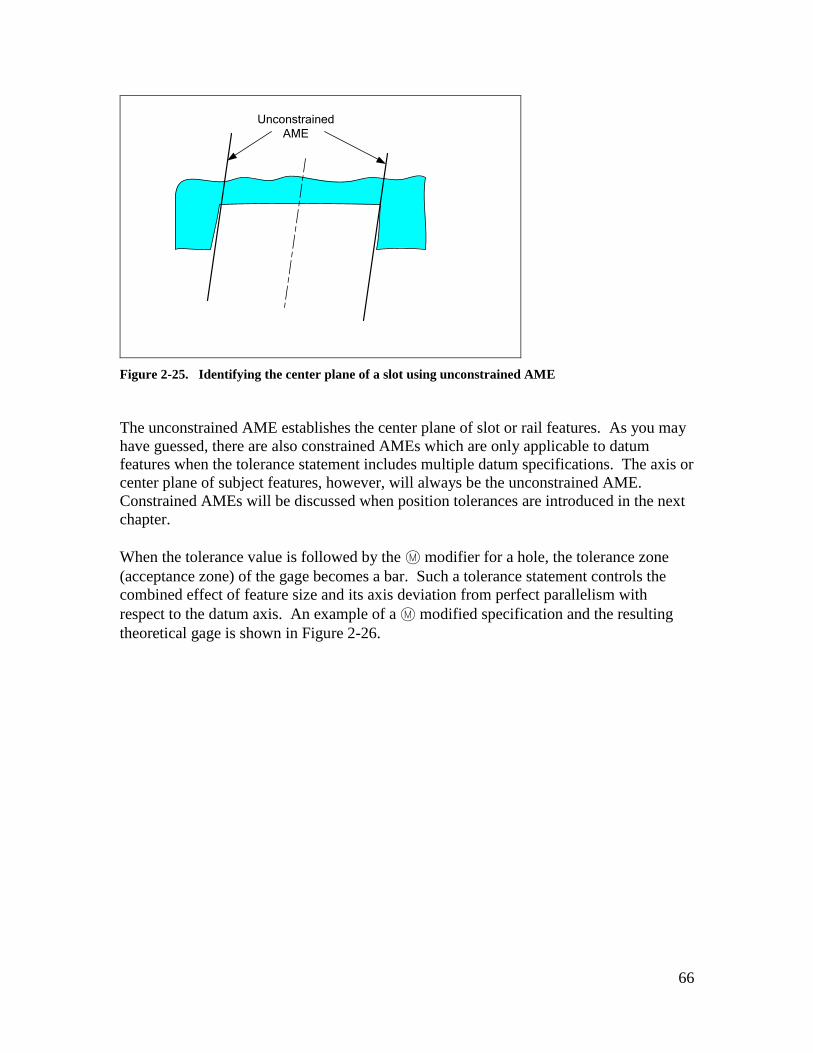
66

Unconstrained

AME

Figure 2-25. Identifying the center plane of a slot using unconstrained AME

The unconstrained AME establishes the center plane of slot or rail features. As you may

have guessed, there are also constrained AMEs which are only applicable to datum

features when the tolerance statement includes multiple datum specifications. The axis or

center plane of subject features, however, will always be the unconstrained AME.

Constrained AMEs will be discussed when position tolerances are introduced in the next

chapter.

When the tolerance value is followed by the m modifier for a hole, the tolerance zone

(acceptance zone) of the gage becomes a bar. Such a tolerance statement controls the

combined effect of feature size and its axis deviation from perfect parallelism with

respect to the datum axis. An example of a m modified specification and the resulting

theoretical gage is shown in Figure 2-26.

67

Ø 0.3 A

40.0 – 40.5

Ø 39.7

Axis-A

M

Figure 2-26. A specification and the resulting gage when the m modifier is used on a hole subject

feature

After aligning the datum simulator axis of the gage with the actual datum feature axis

through an expanding pin, the hole feature must fit over the gage acceptance zone

(yellow pin). The acceptance zone is free to translate parallel to the datum axis. The size

of the pin for a hole feature is 39.7mm which is equal to the smallest hole size (40 mm)

minus the tolerance value (0.3 mm). When the actual hole is made to be larger (closer to

40.5 mm), the gage automatically allows it to be less parallel relative to the datum axis.

When the pin is closer to 40 mm its axis has to be more parallel relative to the datum

axis.

2.14. Perpendicularity

Perpendicularity requires a surface or axis to be perpendicular to another reference

surface or axis to within a specified tolerance value. The reference surface or axis is

labeled as a datum. Figure 2-27 shows an example in which an axis is specified to be

perpendicular to a planar feature.

68

Figure 2-27. An example of perpendicularity tolerance specification

The interpretation of perpendicularity tolerance statement is similar to that of parallelism.

The only difference is that the tolerance zone of the gage is perpendicular to the datum

simulator plane or axis. The theoretical gage for the perpendicularity statement of Figure

2-27 is shown in Figure 2-28.

69

Datum Simulator

Cylindrical

Tolerance

Zone

0.3

Figure 2-28. The theoretical gage for axis perpendicularity statement

The gaging process requires placing the datum feature of the part against the datum

simulator and checking the axis of the boss feature for containment within the 0.3 mm

diameter tolerance zone. The axis of the boss subject feature is established by its

unconstrained AME.

If an m modifier follows the tolerance value of Figure 2-27, the acceptance zone of the

gage becomes a hole of size 30.35 mm. The gage controls the combined feature size and

perpendicularity. Figure 2-29 shows the resulting gage and an example of gaging. The

outline of an actual part is shown in red. This feature fits the acceptance zone of the gage

while fully resting on the datum simulator.

70

Datum Simulator

The Gage

Gaging

30.35

Figure 2-29. The theoretical gage for axis perpendicularity statement when tolerance value is

followed by an m symbol

Note that the gage allows a pin made closer to its LMC size of 30 mm to have a larger

orientation deviation than a pin closer to its MMC size of 30.05 mm.

2.15. Angularity

Angularity requires a surface or axis to be at a certain orientation relative to another

reference surface or axis to within a specified tolerance value. The reference is identified

as a datum. Figure 2-30 shows a typical use of angularity for a planar feature.

71

Figure 2-30. An example of angularity tolerance statement

The gage for this angularity tolerance specification is shown in Figure 2-31.

Datum Simulator

28

0.1

The zone can

translate

Figure 2-31. Theoretical gage for the angularity tolerance

The interpretation of angularity follows the same procedure as parallelism and

perpendicularity. For the angularity statement shown in the figure, the tolerance zone is a

72

pair of parallel planes with a 0.1 mm separation. This tolerance zone is oriented at an

angle of 28 degrees relative to the datum simulator plane of the gage.

Exercise Problems

1. Model the turning support part in a CAD system and create a drawing sheet as shown

in Figure 2-32, excluding the labels.

Figure 2-32. Turning support part

Using GDT standard annotation capacities of the CAD system, specify the following

tolerances:

a. Define plane P1 as Datum-A.

b. Define slot S1 as Datum-B.

c. Define plane P2 as Datum-C.

d. Make Datum-A feature flat to within 0.02 mm.

e. Make Datum-B perpendicular to Datum-A to within 0.05 mm.

f. Make Datum-C perpendicular to Datum-A and Datum-B to within 0.1 mm.

g. Specify the size limits of hole H1 to be 20 ±0.02 mm.

h. Specify the size of slot S1 to be 76.00 – 76.15 mm.

i. Specify the size of holes H2 to be 12.00 – 12.25 mm.

j. Specify hole H1 to be parallel to plane P1. Use a tolerance value of 0.1 mm.

73

2. Consider the turning support part shown in Figure 2-33. Draw the theoretical gages

for the following:

a. The flatness specification.

b. The circularity specification.

c. The parallelism specification.

d. The perpendicularity specification.


3. Consider the turning support part shown in Figure 2-34. Draw the theoretical gages

for the following:

a. The straightness specification.

b. The parallelism specification.

c. The perpendicularity specification.

d. The cylindricity specification.

74


4. Consider the part shown in Figure 2-35.

A

B

12.5

3 B

2 A

Figure 2-35. A 2D part drawing

The real part is shown in Figure 2-36.

a. Create theoretical gages for the two tolerance statements.

75

b. Draw the perpendicularity gage for the slot feature on a transparency and

check the real part for conformance. Is the orientation of the slot acceptable?

c. Draw the perpendicularity gage for the planar feature on a transparency and

check the real part for conformance. Is the orientation of the planar feature in

the perpendicularity statement acceptable?

Figure 2-36. A 2D manufactured part

5. Consider the specifications shown in Figure 2-37.

a. Draw the gage for perpendicularity on a transparency and check for

conformance.

b. Is the perpendicularity of the plane acceptable?

c. Check the circularity of the hole feature by drawing the circularity gage on a

transparency and comparing it against the real part.

A

B

12.53 B

1

Figure 2-37. A 2D part drawing

76

Figure 2-38. A 2D manufactured part

77


Tolerance Statements - Part-II

3.1. Overview

This chapter presents the meaning of the remaining important tolerance statements

including tolerances of location and profile tolerances. A gage that defines a tolerance of

location must use at least one location dimension for its construction. Sometimes the

location dimension is zero when the features are aligned such as with coaxial features.

The location dimensions can also be the distances within a pattern of features.

3.2. Tolerances of location

Tolerances of location control the distance between a subject feature and one or more

datum features. Tolerances of location fall into one of the types shown in Table 3-1.


Use

Position tolerance Single or pattern of cylinders

Single or pattern of width features *****

Circular runout Circular cross-sections (2D) *****

Total runout Cylindrical features ***

Concentricity Circular cross-sections (2D) *

Symmetry Cross-sections (2D) *

Table 3-1. Tolerances of location

3.3. Position tolerance

Position tolerance may be applied to features-of-size or their patterns. A pattern of

features must have features with identical sizes and usually with identical functions. For

single features, position tolerance requires the axis (or center plane) of a subject feature

to be within a specified tolerance zone with respect to a datum frame. For patterns of

features, the position statement additionally requires the relative locations within the

pattern to be maintained with the same accuracy. The presentation here uses cylindrical

subject features but the position tolerance also applies to width features. For width

features, center planes substitute for the axes of cylindrical features.

Figure 3-1 shows a simple part with a position control statement. Assume the parts

shown are plates with a constant thickness.

78

A

B

Ø 1 A B

15-16

50

20

Figure 3-1. Position tolerance applied to a single cylindrical feature

The theoretical gage for this position tolerance specification is shown in Figure 3-2.

Datum-A and datum-B are datum feature simulators.

1-mm diameter

tolerance zone Basic

Position

Datum-A

Datum-B

50

20

Figure 3-2. The gage for the position tolerance applied to a single cylindrical feature

Since the position tolerance applies only to features-of-size the tolerance value can

always be followed by an m or l modifier. The position tolerance statement with

79

modifiers are used to control the combined effect of size and position deviation. Figure

3-3 shows an example of an m-modified tolerance value.

A

B

Ø 1 A BM

50

20

15-16

Figure 3-3. An example of an m modified position tolerance specification

For an m-modified tolerance statement, the acceptance zone of the gage becomes a boss

as shown in Figure 3-4. The size of the boss is equal to the minimum size of the hole (15

mm) minus the tolerance value (1 mm) resulting in a 14 mm boss. The gage allows a

hole closer to its LMC size of 16 mm to deviate more from the theoretical position than a

hole made closer to its MMC size 15 mm.

80

14

Basic

Position

50

20

Datum Simulator

Datum Simulator

Figure 3-4. The tolerance zone is located at the basic position with respect to the datum frame

When multiple datum features are used in a tolerance statement, datum references are

placed in the tolerance control box and their order or priority is assigned from left to

right. The datum priority makes a difference in the manner of gaging but the gage itself

is unaffected by the datum ordering. Up to three datums can be referenced in a position

tolerance statement. The first datum is called the primary datum, the next one, if

specified, is the secondary datum, and the third one, if specified is the tertiary datum.

The datum features and datum priority mimic the way the part is intended to be fixed to

an assembly. Figure 3-5 shows a final desired arrangement of a part into an assembly.

Figure 3-5. The intended arrangement of part contact to the mating part

81

Each datum reference in a tolerance statement leads to a corresponding datum simulator

on the theoretical gage. These datum simulators represent the perfect-form and perfect-

orientation mating surfaces. The procedure for constraining the part to the gage is stated

through the order of datum specification and illustrated in Figure 3-6.

Primary Datum

Simulator Plane

Secondary Datum

Simulator Plane

Secondary

Datum

Feature

Primary Datum

Feature

Figure 3-6. The procedure for constraining the part against datum simulators

The primary datum simulator makes full unconstrained contact with its datum feature on

the part. The secondary datum contact would not have an unconstrained contact because

the part is required to remain in contact with the primary datum simulator. If the

manufactured part had perfectly perpendicular datum features, then the datum priority

would have made no difference when placing the part into assembly.

Figure 3-7 shows the actual arrangement of the part relative to the datum simulators

when the datum priority is reversed. This change of datum priority leads to a completely

different part staging. In this case, datum-B surface orients the part.

82

Primary Datum

Simulator Plane

Secondary Datum

Simulator Plane

Figure 3-7. The actual arrangement of part against the datum simulators when the side plane is the

primary datum

Once the part is constrained to the datum simulators, the subject feature axis can be

checked against the tolerance zone of the theoretical gage as shown in Figure 3-8. The

basic position is the theoretical position of the hole axis with respect to the datum frame.

The basic position is where the axis should be for a perfect placement.

50

20

Figure 3-8. The tolerance zone is located at the basic position with respect to the datum frame

83

In the case of Figure 3-8, the hole position is out of tolerance. Since simulators represent

the mating surfaces on which the part contacts, the selection of the datum priority is such

that it mimics the final assembly. When a part is being installed into an assembly it can

only make full unconstrained contact on one surface. The next contact is going to be

partially constrained by the first primary contact. For example, if datum-A plane is fixed

to its mating plane by screws, then datum-A plane would be the primary datum. If

datum-B plane is screwed to its mating part when it is installed in the assembly, then

datum-B plane should be specified as the primary datum. If the design requires both

surfaces to be screwed to mating surfaces, then the datum surfaces must be specified to

be perpendicular with high precision. In that case it makes no difference which datum is

selected to be the primary datum.

Figure 3-9 shows another example of a position tolerance involving a bearing hole

controlled with respect to two datum references. The 25H7 designation is a coded way

of stating the size limits of the hole. The 25H7 numerical limits are 25.000 – 25.021 mm.

Coded size limits will be presented later in Chapter-6.

Figure 3-9. An example of position tolerance statement

In this example, datum-A is the primary datum. Datum-B, the secondary datum, is the

center plane of the slot. To specify the center plane as the datum, the datum symbol

must be aligned and attached to the dimension line. The axis of the bearing hole is

84

required to be parallel to and at a precise distance from datum-A. The bearing hole is

also required to be centered relative to the slot center plane identified as datum-B. The

datum simulator for datum-A is a plane and the datum simulator for datum-B is a pair of

expanding jaws that grip the part. The expanding pair of jaws, however, must remain

perpendicular to the primary datum-A simulator as the jaws open. Rather than showing

the expanding pair of jaw datum simulators, the center plane of the expanding jaws will

be shown in the theoretical gages. The theoretical gage for this statement is shown in

Figure 3-10.

Figure 3-10. The theoretical gage

In the theoretical gaging procedure, which is shown in Figure 3-11, first the bottom

surface of the part is pressed against the datum-A simulator of the gage just like a part is

placed into a mating part surface of an assembly. Next, the parallel jaws of datum-B

simulator grip the part as they open to fit inside the slot datum feature. The datum-B

simulator mimics the slot fitting tightly into a mating rail.

85

Figure 3-11. Theoretical gaging procedure requires constraining the part to the datum planes and

checking the subject feature axis for containment within the tolerance zone

Figure 3-12 shows a pair of expanding jaws (parallel planes) gripping the slot. The

resulting boundary (when the jaws can no longer expand) is the orientation-constrained

actual mating envelope (orientation-constrained AME) of the slot.

Datum A

Orientation

Constrained AME

Figure 3-12. The orientation-constrained actual mating envelope for a slot

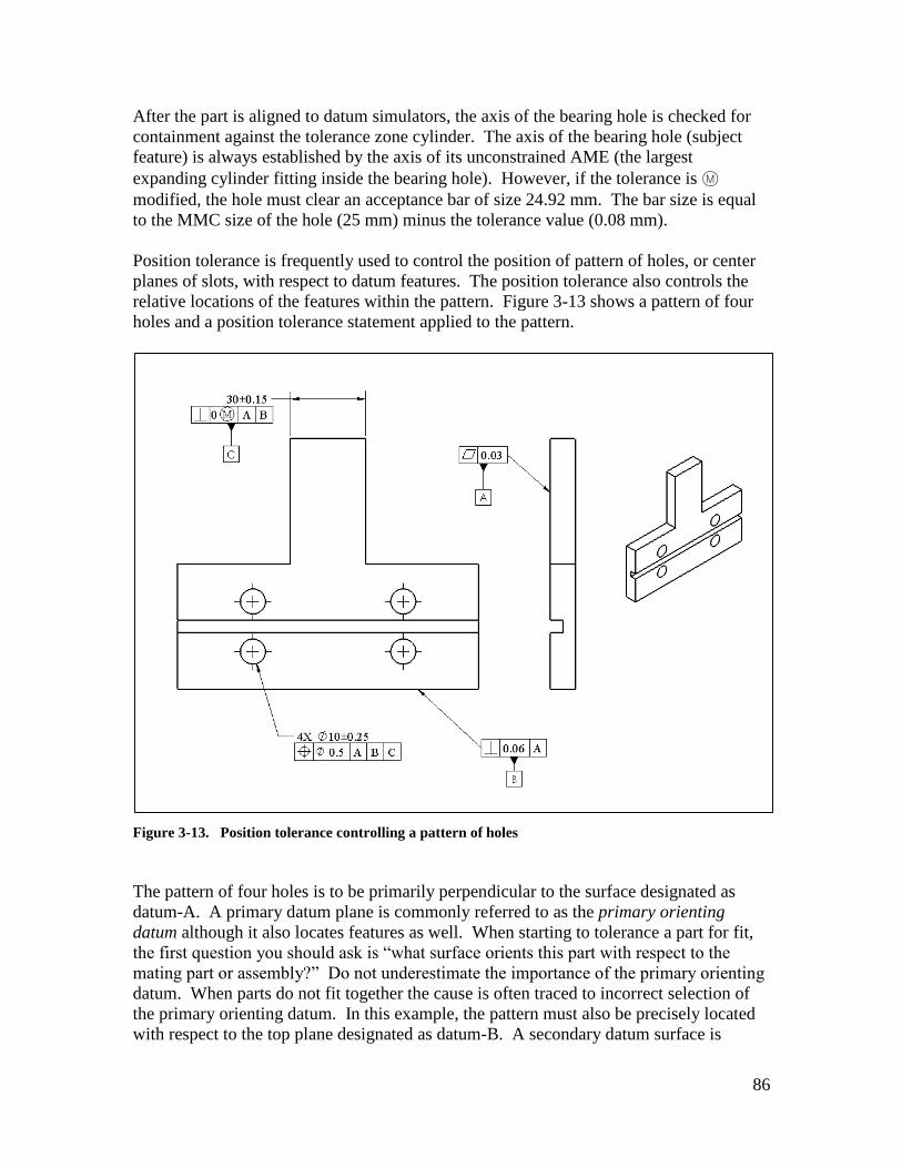
86

After the part is aligned to datum simulators, the axis of the bearing hole is checked for

containment against the tolerance zone cylinder. The axis of the bearing hole (subject

feature) is always established by the axis of its unconstrained AME (the largest

expanding cylinder fitting inside the bearing hole). However, if the tolerance is m

modified, the hole must clear an acceptance bar of size 24.92 mm. The bar size is equal

to the MMC size of the hole (25 mm) minus the tolerance value (0.08 mm).

Position tolerance is frequently used to control the position of pattern of holes, or center

planes of slots, with respect to datum features. The position tolerance also controls the

relative locations of the features within the pattern. Figure 3-13 shows a pattern of four

holes and a position tolerance statement applied to the pattern.

Figure 3-13. Position tolerance controlling a pattern of holes

The pattern of four holes is to be primarily perpendicular to the surface designated as

datum-A. A primary datum plane is commonly referred to as the primary orienting

datum although it also locates features as well. When starting to tolerance a part for fit,

the first question you should ask is “what surface orients this part with respect to the

mating part or assembly?” Do not underestimate the importance of the primary orienting

datum. When parts do not fit together the cause is often traced to incorrect selection of

the primary orienting datum. In this example, the pattern must also be precisely located

with respect to the top plane designated as datum-B. A secondary datum surface is

87

commonly referred to as the secondary locating datum. Finally, the pattern must be

precisely centered with respect to the center plane of the rail feature designated as datum-

C sometimes called the tertiary locating datum. Figure 3-14 shows the resulting

theoretical gage. Do not be alarmed by the zero tolerance value in the perpendicularity

tolerance. A zero geometric tolerance value is not an error when used with an m or l

modifier.

Figure 3-14. The theoretical gage for inspecting the pattern position tolerance statement

The gage is composed of three mutually perpendicular planes. Datums-A and datum-B

are contacting datum simulators while datum-C represents the center plane of collapsing

jaws that grip the datum-C rail. The pattern of four tolerance cylinders has a theoretical

distance relationship with datum-B and datum-C planes. Tolerance cylinders have 0.5

mm diameters. Figure 3-15 shows how the gage is aligned to the part to check the

position accuracy of the hole pattern. The datum simulator for the rail feature, datum-C,

is a pair of collapsing jaws that must remain perpendicular to datum simulator plane A

and datum simulator plane B. The theoretical gage shows the center plane of the jaws

after they fully grip the part.

88

Figure 3-15. The theoretical gaging for inspecting the pattern position tolerance statement

In this example the datum frame completely fixes the part to the gage. Judging from

Figure 3-15, two of the holes in the pattern are clearly off position. Figure 3-16 shows

the datum simulators of a physical gage.

Figure 3-16. A physical gage showing only the three datum simulators

89

If an m modifier follows the tolerance value as indicated in Figure 3-17, the tolerance

zones change to a pattern of acceptance bars. The m modified specification controls the

combined effect of size and position deviations. The gage automatically allows larger

holes to be off position more than the smaller holes.

Figure 3-17. Position tolerance controlling a pattern of holes using m modifier

The resulting theoretical gage is shown in Figure 3-18. The gage appears more realistic

now as a mating part compared to the gage with tiny laser beam tolerance zones. The

size of each bar is 9.25 mm.

90

Figure 3-18. The theoretical gage for the m modified pattern position tolerance

Figure 3-19 shows the theoretical gage and the gaging process. The hole features are

acceptable if they all clear the gage bars.

Figure 3-19. The theoretical gaging for inspecting the pattern position tolerance statement

A physical gage simulating the theoretical gage and the gaging procedure can be

constructed as shown in Figure 3-20. The loose pins are used to make the physical

gaging practical.

91

Figure 3-20. A physical gage for inspecting m modified position tolerance

After the part is placed on the datum-A simulator plane and pushed against datum-B, the

jaws move to grip the part to complete datum alignment or staging. As the jaws grip the

part the part must remain in full primary contact with datum-A surface and secondary

contact with datum-B surface. The inspector then attempts to insert the pins into their

sockets that have the same sizes as the pins. If all the pins fit into their sockets, the

pattern geometry is acceptable regarding the position tolerance. The jaws must be

designed such that they move together the same amount. This ensures the hole pattern

will always remain centered to the jaw’s center plane.

3.4. Meaning of m modifier applied to datum features It was mentioned that datums simply mimic the constraining surfaces of an assembly as

the part is placed into the assembly. When a datum feature referenced in a tolerance

statement is a feature-of-size and intended to fit a mating feature, it is most likely a rigid

feature. The designer can apply a material condition modifier to such a datum. When an

m modifier follows the datum label in the tolerance statement, the datum is said to apply

at its maximum material boundary (MMB). An example is shown in Figure 3-21.

92

Figure 3-21. A position tolerance statement with an MMB datum specification

A referenced datum feature with an m material condition modifier establishes a fixed

size datum simulator. The size of the datum simulator is determined using the same

formula as the size of m modified subject feature acceptance zones were determined. In

this case, the size of the datum simulator slot for datum-C is 30.15 mm. The size of

datum-C is obtained by adding the rail’s MMC size of 30.15 mm to its tolerance of zero

at MMC. Figure 3-22 shows the physical gage for the inspection of the part with MMB

specification for datum-C. As you can see this is a more realistic representation of a

mating part compared to one with the expanding jaws.

93

Figure 3-22. A physical gage for inspecting position tolerance with m modified datum

The purpose of applying an m modifier to a datum feature is to allow any slack in the

datum fit to compensate for inaccuracies of the subject feature pattern during assembly

by adjusting the datum fit. In this case, any slack in the fit between the actual datum-C

feature and the gage can be used to compensate for the feature pattern shift provided that

such an adjustment can be made during assembly.

3.5. Composite position tolerance – multiple segments

In the example previously shown in Figure 3-13, a single position statement controlled

the location and orientation of holes within the pattern and with respect to datums A, B,

and C. After the part is fixed to a mating part using the stated datum frame, the designer

may want to apply additional precision requirements to the same pattern of features. To

control the position and orientation of a pattern more precisely another position control

statement can be added to the original specification. This additional position tolerance,

which has a smaller tolerance value, also controls the relative position of the holes with

respect to each other with more precision. This type of position tolerance is called

multiple segment composite position tolerance and only applies to feature patterns.

Figure 3-23 shows a multi-segment composite position tolerance. Note that there is a

separate position tolerance symbol for each statement. The upper segment controls the

pattern position with respect to the three datum planes as before. The lower segment

94

controls the position of the pattern more precisely with respect to two datums, datum-A

and datum-B. It also controls the relative location of the features within the pattern with

more accuracy.

Figure 3-23. The multiple segment composite position tolerance statement

Figure 3-24 shows the gage for the composite tolerance. The gage now includes the 0.25

mm tolerance zone pattern (shown in green) that is not centered with respect to the rail

(datum-C) and therefore is free to slide while maintaining its basic distance to datum-B.

95

Figure 3-24. The theoretical gage for multiple segment composite position tolerance statement

Figure 3-25 shows the gage for the lower statement. The designer controls the pattern

location more closely with respect to datum-A and datum-B without needing the

additional level of precision with respect to datum-C. The circles represent the tolerance

zones. The arrows show that the tolerance zones can translate as a whole to the right or

left (parallel to datum-B) but not up and down (toward datum-B).

Datum-B

Theoretical

Distance

A Ø 0.25

Figure 3-25. The theoretical gage for inspecting the pattern position with respect to datum-A and

datum-B

96

If the tolerance values are m modified, the tolerance zones will become acceptance bars

of size 9.5 mm for the upper position statement. The specification then controls the

combined effect of size and position deviation. For an m modified lower specification,

the 0.25 mm tolerance zones become 9.75 mm acceptance bars.

If the two statements with the composite format are applied independently as two

unconnected statements, then each one would have resulted in a separate gage. The

difference is that in the composite format all statements use the same datum alignment

with the simulators. This becomes important when one or more of datum features is

called out at MMB which allows multiple possible alignments to the datum features

during inspection. In practice, the idea is that once a part is placed into an assembly

using a particular alignment with the datum features, that alignment cannot be changed

when checking the lower statement.

A theoretical inspector first aligns the datum frame with the part datum features and then

checks the red tolerance zones associated with the upper tolerance segment. If the pattern

passes this stage, the inspector discards the red tolerance zones and slides in the green

lower segment tolerance zones to check the lower segment.

Note that in order for the two attached position tolerance statements to be considered a

composite tolerance, the datum frame must be repeated exactly in the lower segment,

including its order, but usually with fewer datum references. If the datum frame does not

repeat exactly in the lower segment, the two statements are interpreted as two

independent position tolerance statements.

If the designer intends to make the pattern position even more precise in terms of being

square to datum-A and also for the relative positions within the pattern, a third statement

can be added to the composite position statement using only datum-A reference. This

leads to a gage with a third pattern of tolerance zones with even smaller tolerance zone

cylinders. Three-segment composite tolerance statements, however, are not common.

3.6. Composite position tolerance – single segment

A composite position tolerance can be specified in which a single position tolerance

symbol is shared by multiple statements. This is called a single-segment composite

position tolerance format. An example is shown in Figure 3-26.

97

Figure 3-26. A single-segment composite position tolerance statement

In a single-segment position tolerance format, the upper statement is interpreted as in the

multi-segment format. The upper statement locates the pattern with respect to the datum

features as before. The lower segment, on the other hand, only controls the orientation of

the pattern with respect to the specified datum frame as well as the relative location of the

feature pattern members. Figure 3-27 shows the tolerance zones resulting from the lower

statement of the single-segment tolerance specification. The hole pattern need not be

located to datum-B anymore as long as it remains parallel to datum-B. The upper

segment still controls how far the pattern can translate toward or away from datum-B.

98

Datum B

A Ø 0.25

Figure 3-27. The theoretical gage for inspecting the pattern position with respect to datum-A and

datum-B in a single-segment specification

For example, the lower segment in Figure 3-26 controls the orientation of the pattern

more precisely with respect to datum-A and datum-B. The lower statement also controls

the relative location of the pattern features with more accuracy relative to one another.

The result of the composite statement is that the pattern is allowed to translate toward or

away from datum-B more but it is not allowed to rotate as much. The theoretical gage for

this statement is identical to the one for multiple-segment position tolerance format

except that the tolerance zone associated with the lower segment is not located and is free

to translate away or toward datum-B.

In order for the two position tolerance statements to be considered a composite tolerance,

the datum frame must be repeated exactly in the lower segment, including its order and

modifiers. If a designer intends to make the relative locations within the pattern even

more precise and more perpendicular to datum-A, a third statement can be added to the

composite position statement using only datum-A reference. This leads to a gage with a

third pattern of tolerance zones having smaller size tolerance cylinders.

3.7. Runout tolerances

Circular Runout

Circular runout requires feature cross-sections to be circular in form and concentric to the

axis of a feature selected as datum, to within the specified tolerance value. Circular

runout is primarily used to control the coaxiality of shaft cross-sections relative to an axis

of rotation. Figure 3-28 shows the shaft assembly of a gearbox. In this application, it is

important for the gear’s fitting surface to be coaxial to the axis of rotation defined by the

99

two bearings. Otherwise, the gear teeth will wobble radially in and out shortening the life

of the gear.

Figure 3-28. A rotating part that requires coaxiality of its features with respect to the axis of

rotation defined by the bearings

Figure 3-29 shows how this type of tolerance control can be specified using circular

runout specification. The 10k6 and 10h9 codes define the feature size limits. The

application of these size codes will be covered in Chapter-6.

Figure 3-29. An example of coaxiality control through circular runout statement

100

Datum-A defines the axis of the smaller bearing fit cylinder. The larger bearing fit

cylinder is controlled to be coaxial to datum-A with high precision using circular runout

specification. The axis of the larger bearing cylinder is identified as datum-B. The

gear’s fit surface is specified to be coaxial to an axis defined by the two bearing axes

simultaneously. Other than lack of coaxiality, lack of circularity also influences circular

runout.

The primary datum in circular runout specification is always an axis obtained by a

collapsing (or expanding) datum simulator. The tolerance zone is the 2D zone defined by

a pair of concentric circles with a radial thickness equal to the specified tolerance as

shown in Figure 3-30. The tolerance zone is similar to circularity zone but there is an

added datum axis in the center of the circles.

datum axis

simulator

tolerance zone

The plane of cross-section

(cutting plane)

0.05

Figure 3-30. Theoretical gage for circular runout consists of two concentric circles and an axis on a

planar surface

In the theoretical inspection, the two collapsing holes for the datum features

simultaneously grip the part. Then the plane of the cross-section cuts the part

determining the intersection profile of the gear surface with the cutting plane. This is


101

plane of cross-section

(cutting plane)

intersection profile

Figure 3-31. Theoretical gage for circular runout and the cross-section of the subject feature

In this case, the cross-section is circular enough but it is off center with respect to the

datum axis. Circular runout specification is easy to verify using a simple inspection set

up such the one shown in Figure 3-32.

Datum

Figure 3-32. The most common method of verification of circular runout statement

To do the physical inspection, the part ends are fixed in rotating chucks (collapsing

cylinders). These chucks locate the center of rotation and establish the datum axis. The

chucks are simultaneously tightened so neither of the datum cylinders is favored. The

plane of the dial indicator simulates the cutting plane. The dial stem is perpendicular to

the axis of the chuck and radially aligned with it. The part is then rotated with the dial

indicator set up to measure radial deviations. As the part rotates, the full movement of

the indicator (FIM), or the range of the dial travel, measures the runout of the cross-

section relative to the axis of rotation. If this measured runout is smaller than the

102

tolerance value, the measured cross-section is within tolerance. For checking another

cross-section, the dial is moved to that cross-section and the process is repeated. Unless

otherwise indicated on the drawing as a note adjacent to the runout specification, the

runout applies to all cross-sections of the feature.

Circular runout can also be used to control the perpendicularity of shaft shoulders with

respect to the axis of rotation. This is the specification of choice when controlling shaft

shoulders that support bearings, gears, or other shaft components. Figure 3-33 shows an

example.

10 10

A B

0.1 A-B

Figure 3-33. An example of shoulder perpendicularity control through circular runout statement

Circular runout specification applied to planar surfaces is also easy to verify using a

simple inspection set up such as the one shown in the top of Figure 3-34.

103

Datum

axis

A little

circular

runout

A lot of

circular

runout

Figure 3-34. The most common method of simulating the theoretical gage for the verification of

circular runout statement

Unless otherwise specified, the specification applies independently to all circles on the

subject plane. That means the dial indictor test must be applied at various circle sizes.

When the surface bulges out or in, as shown in the part in the middle of the figure, no

runout would register on the dial. The function of a bearing or a similar component that

is fitted to a rotating shaft is not adversely affected by this kind of surface. The part in

the bottom of the figure is unacceptable and, when tested, shows a lot of runout. This

kind of surface forces the bearing or the component to rotate relative to the axis of

rotation.

If you are curious to know, the theoretical gage for the specification in Figure 3-33 is a

strip of cylindrical surface and a datum axis as shown in Figure 3-35. The axial length of

the strip is the tolerance value. The strip is free to translate along the datum-A axis. The

diameter of the cylinder corresponds to the location along the shoulder where the runout

is checked.

104

Datum-A

0.1

Theoretical Gage

Figure 3-35. The theoretical gage for circular runout applied to a planar surface is a cylindrical

surface

To check the part against this gage, the axis labled datum-A is aligned with the actual A-

B datum of the part. Then, the cylindrical tolerance zone surface cuts the subject plane

and creates a curve of intersection. That curve of intersection must then fit inside the

tolerance zone of the theoretical gage.

Total runout

Total runout requires features to be cylindrical in form and coaxial with respect to the

axis of a feature selected as datum to within a specified tolerance value. Figure 3-36

shows the roller assembly of a machine. For functional reasons it is important to have a

precisely uniform distance between this roller and an opposing roller or plate as the roller

turns. This type of precision requires total runout specification which controls the

combined tolerances of cylindricity and coaxiality.

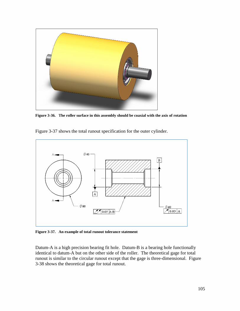
105

Figure 3-36. The roller surface in this assembly should be coaxial with the axis of rotation

Figure 3-37 shows the total runout specification for the outer cylinder.

Figure 3-37. An example of total runout tolerance statement

Datum-A is a high precision bearing fit hole. Datum-B is a bearing hole functionally

identical to datum-A but on the other side of the roller. The theoretical gage for total

runout is similar to the circular runout except that the gage is three-dimensional. Figure

3-38 shows the theoretical gage for total runout.

106

Datum Axis

Tolerance

Zone

Figure 3-38. Theoretical gage for total runout consists of two concentric cylinders and an axis

During gaging, the datum axis of the gage is aligned with the axis of the datum feature

using collapsing cylinders. The cylindrical subject feature is then checked against the

tolerance zone. Total runout specification is also easy to verify using the simple

inspection set up used for circular runout as shown in Figure 3-39.

Datum

Figure 3-39. The most common method of simulating the theoretical gage for the verification of a

total runout statement

Compared to circular runout, the only difference is that once the dial is set in the

beginning, the full indicator movement (FIM) includes the range of movement as the

indicator is moved to other cross-sections. The total runout is measured as the FIM of the

dial. Total runout applied to a shaft shoulder is identical to perpendicularity tolerance

with respect to the datum axis.

107

3.8. Profile tolerances

A surface profile is the general term used to refer to any type of surface or any selected

group of surfaces. A profile feature’s size, form, orientation, and location can be

controlled using one or more profile statements. The surface profile statement is a good

replacement for the traditional ± tolerances for features not involved with fit. The ±

tolerances should still be used for size tolerances with features-of-size in fit applications.

Profile of a surface tolerance d

Profile of a surface tolerance is the general-purpose surface feature control specification

of the GDT standard. Profile tolerance can be applied to surface features of any shape

including any grouping of features. In fact, the entire outer skin of a part is an important

profile feature that is commonly controlled in default tolerancing.

The profile of a surface tolerance controls one or more surface features to remain within a

thin envelope around their basic or theoretical shape. This thin envelope is the tolerance

zone geometry. The profile tolerance is often used with a datum frame to control both

the size and the location of a profile. Figure 3-40 shows two examples. The circle

attached to the arrow is the “All Around” symbol indicating that the tolerance statement

applies to all the surfaces making up the inner profile, or the outer profile of the turning

support part. The dimensions are theoretical dimensions and are shown here to explain

the gage geometry.

Figure 3-40. Examples of profile of surface tolerance specifications

108

The tolerance statement controls the size of the entire shape. The feature is also located

and oriented relative to the bottom surface (datum-A) and it is centered relative to the slot

center plane (datum-B). The theoretical gage for this specification is shown in Figure 3-

41. The 0.3 mm tolerance zone has a depth larger than the thickness of the part.

Figure 3-41. Theoretical gage for profile statement

The profile tolerance can also be specified to be unequally divided about the theoretical

profile geometry using a simple notation. Figure 3-42 shows an example. If the profile

tolerance is to be divided such that 0.1 mm is allocated in the direction of adding material

to the theoretical shape, the tolerance value of 0.3 U 0.1 should be specified. The first

number is the total thickness of the tolerance zone and the second number is the thickness

of the portion that adds material to the part. The dashed line in the figure represents the

theoretical profile shape.

109

Datum A

0.3 U 0.1 A B

0.3

50

300.1

Figure 3-42. An example of unequally divided profile tolerance specification and the resulting

tolerance zone

The specification 0.3 U 0.3 defines the entire tolerance zone in the direction that adds

material to the part. The specification 0.3 U 0 defines the entire tolerance zone in the

direction that removes material from the part.

Composite profile statements can be used to control various geometric aspects of a

profile with finer levels of precision. Composite profile tolerances use the single segment

format in which one profile tolerance symbol is shared by multiple statements. Each

statement must use a progressively smaller tolerance value. For example, consider the

specification in Figure 3-43.

110

Figure 3-43. An example of a composite profile tolerance with two statements

The upper profile statement controls the size, form, orientation, and location of the

feature with an accuracy of 0.3 mm relative to datum-A and datum-B. The lower

statement controls the size and orientation relative to datum-A with the finer accuracy of

0.2 mm.

The theoretical gage for this statement uses the same datum simulators for both the upper

and the lower statements. Once the upper statement is verified, the 0.3 mm tolerance

zone is removed and a new 0.2 mm tolerance zone is brought in without changing the

part alignment to datum-A simulator. The new tolerance zone is parallel to the datum-A

surface. If it is important to additionally control the size of the profile with finer

accuracy a third row of specification can be added with a smaller tolerance value and

without any datum reference.

All profile tolerances control the profile size by creating tolerance zones that are equally

or unequally disposed about the theoretical profile. The only exception, according to the

GDT Standard, is with the control of conical surfaces in which dimension limits can be

used to control the cone size and a profile tolerance can be used to control the cone form.

It is important, however, to be able to control profile form, orientation, or location

separately from profile size for all features. To do this, a word or a symbol can be placed

111

next to the profile tolerance statement and explained as a note. In this book the word

FORM is used for this purpose. The following note should then be added in the drawing

notes section to explain the meaning of the tolerance statement:

FORM: The actual profile must lie within a tolerance zone defined by a pair of

profile surface offsets with a separation equal to the tolerance value

If the profile tolerance is used with an orienting datum reference the FORM designation

would control the form and the orientation of the profile. If the profile tolerance is used

with an orienting and a locating datum reference the FORM designation would control

the form, the orientation, and the location of the profile. Figure 3-44 shows a

specification example. The form control statement can also be added as a third statment

in the composite statement format.

Figure 3-44. Adding a statement for profile form control

For profile form control shown in the figure, the tolerance zone has a thickness of 0.1 mm

but the zone size can expand or contract within the limits of size similar to other form

control specifications such as cylindricity. If the form control (i.e. the text FORM) is

applied to the lower statement with 0.2 mm tolerance value then the profile size would be

dictated by the 0.3 mm zone while the profile combined orientation and form remain

within the smaller 0.2 mm zone.

112

3.9. Profile tolerances in place of ± tolerances

When the distance between two parallel planes is to be controlled the use of profile of

surface tolerance is preferred to the use of ± limits on dimensions unless the feature is a

fit feature (it has opposing planes and fits a mating feature). Consider the shaft in Figure

3-45. The 20 mm distance between two of the shaft shoulders needs to be controlled. In

this specification, the indicated feature dimension is to be between 19 and 21 mm.

20 +/- 1

Figure 3-45. The distance between the two shoulders is controlled using dimension limits

The meaning of the dimension limits, however, is not clear when the two faces do not

have perfect forms, or are not perfectly parallel. What is “obvious” to one person is not

so obvious to another. Figure 3-46 shows the alternative profile tolerance statement that

is not vague. The figure also shows the theoretical gage resulting from this statement that

allows the two planes be as far as 21 mm or as close as 19 mm similar to the dimension

limits. The profile tolerance alternative is preferred because its interpretation in terms of

an acceptance gage is well defined.

113

1

21

19Theoretical

Gage

20

Figure 3-46. Control of distance between two planes using profile of surface tolerance statement

When controlling the distance between two planes using a profile statement, it is

preferred to specify an origin of measurement. This is shown on the upper part of Figure

3-47. The theoretical gage for this specification is shown in the lower part of the figure.

2 A

21

19

A

20

Theoretical

Gage

Datum-A

Figure 3-47. Preferred way to control of distance between two planes using profile of surface

tolerance statement with specification of origin of measurement

Figure 3-48 shows a shorthand notation for profile specification that does not explicitly

label the datum. The end of the dimension line without an arrow implicitly defines a

datum plane. This format of controlling distances is convenient as it does not require

explicit labeling of the datum.

114

2

20

Figure 3-48. Shorthand specification of profile tolerance with implied datum reference

Profile tolerance can also be applied to control a pattern of features similar to feature

patterns controlled by position tolerance statements.

Profile of a line tolerance k

Profile of a line tolerance is the general-purpose 2D tolerance control specification of the

GDT standard. The profile of a line tolerance can be applied to curve features of any

shape that result from the intersection of a surface profile and a cutting plane. Profile of a

line tolerance can control the size and location of 2D cross-sections of a feature. This

statement is often used to control the size of a feature’s cross-sections with finer accuracy

after a surface profile tolerance is applied. The theoretical gage for profile of a line

statement is a thin envelope around the basic geometric shape of the feature in the plane

of cross-sections. Figure 3-49 shows an example of the use of profile of a line tolerance.

115

Figure 3-49. An example of the profile of a line statement

In this example, the designer has used the profile of a surface statement to control the size

and location of the entire surface feature with a relatively wide 1.2 mm tolerance value.

To control the size of each cross-section with more accuracy, the designer adds a profile

of a line tolerance with a tolerance value of 0.5 mm. The datum-A reference requires the

cutting planes to be parallel to datum-A. If the datum-A is not mentioned, the cutting

planes would be normal to the feature spine. The combined effect of the two profile

statements is that the bar cross-sections are more precise in size but the bar can have a

larger degree of bend or twist as long as it remains within the wider profile of a surface

specification.

Exercise Problems

1. Consider the turning support part shown in Figure 3-50.

116


Specify the following labels and tolerances.

a. Define P1 as datum-A.

b. Define S1 as datum-B.

c. Define P2 as datum-C.

d. Make datum-A feature flat to within 0.02 mm.

e. Make datum-B feature perpendicular to datum-A feature to within 0.05

mm.

f. Make datum-C feature perpendicular to datum-A and datum-B to within

0.1 mm.

g. Specify the size limits of H1 to be 20 ±0.02 mm.

h. Specify the size limits of S1 to be 76.00 – 76.15 mm.

i. Specify the size limits of H2 to be 12.00 – 12.25 mm.

j. Specify H1 to be parallel and located to P1 and aligned with S1. Use a

tolerance value of 0.1 mm.

k. Control H2 to be perpendicular to P1 and aligned to S1. Use a tolerance

value of 0.75 mm and make the specification m modified.

l. Control the orientation of H1 to be more precisely parallel to P1. Use a


117

m. Control the size and location of Prof1 to be parallel to and located to P1

and aligned with S1. Use a tolerance value of 1 mm.

n. Refine the size and orientation precision of Prof1 relative to P1 using a


o. Refine the form and orientation precision of Prof1 relative to P1 using a


p. Refine the form precision of Prof1 using a tolerance value of 0.1 mm.

q. Specify a plate thickness tolerance of 0.5 mm using short-hand profile

tolerance specification using any of the two parallel faces as implicit

datum.

2. Consider the part shown in Figure 3-51. For each tolerance statement in the

following list, draw the theoretical gage and indicate the gage dimensions.

a. The position tolerance specification. Create a theoretical gage with two

different tolerance zones, one for the upper and one for the lower

segments.

b. Theoretical gages for part (a) when the m modifier is used in the tolerance

statements.

c. The profile statement for the inner shape.

d. The profile statement that controls the plate thickness.

118



a) Draw the theoretical gage for the composite position tolerance.

b) Draw the theoretical gage when the m modifier is used with the tolerance

value.

c) Draw the theoretical gage when the m modifier is used both with the

tolerance value and with datum-B.

d) Create the CAD model of a physical gage for part c).

119

Figure 3-52. A part with a pattern of radial holes




value.

c) Draw the theoretical gage when the m modifier is used with the tolerance

value, datum-B, and datum-C.

d) Create the CAD model of a physical gage for part c).

120

Figure 3-53. A part with a pattern of radial holes and a slot




value.

c) Draw the theoretical gage when the m modifier is used with the tolerance

value, datum-B.

d) Read the standard and find out whether the m modifier can be used with

datum-C plane. If the m modifier can be used on datum-C, draw the resulting

gage.

e) Create the CAD model of the physical gage for part d).

121

Figure 3-54. Part with coaxial radial holes

6. Consider the part shown in Figure 3-55. Draw the theoretical gages for all tolerance

statements. Also, draw the theoretical gages when the m modifier is used with

tolerance values.

122

Figure 3-55. Part with U-shaped plate

The symbol CF stands for “continuous feature”. The continuous feature symbol is used

for interrupted surface features and designates the entire surface as the subject feature. In

the case of this problem the datum feature A is the entire planar surface not just the half

the datum label refers to.

7. Consider the 2D part shown in Figure 3-56 and the position tolerance statement

applied to the hole on the top of the figure. The dimensions that define the theoretical

location of the hole are not shown.

a) Create a theoretical gage for this tolerance statement.

b) Create a theoretical gage when the m modifier is used with the tolerance

value.

123

A

B

Ø 3 A BØ20 +/- 1

Figure 3-56. Position tolerance with A as primary datum and B as secondary datum

Consider the manufactured part is shown in Figure 3-57.

c) Is the location of the hole acceptable?

Figure 3-57. The actual part

8. Do the previous problem but this time with the datum priority reversed as shown in

Figure 3-58.

124

A

B

Ø 3 B AØ20 +/- 1

Figure 3-58. Position tolerance with B as primary datum and A as secondary datum

Consider the same manufactured part shown again in Figure 3-59.


9. Consider the position tolerance specification shown in Figure 3-60.

125

A

Ø 3 A BØ20 +/- 1

12 +/- 1

B

Figure 3-60. Position tolerance with datum-B as the slot center plane

a) Create a theoretical gage for this tolerance statement.

b) Create a theoretical gage when the m modifier is used with both the tolerance

value and with datum-B.

c) Is the location of the hole acceptable for each specification?

Figure 3-61 shows the manufactured part.


10. For the specification shown in Figure 3-62

a) Create a theoretical gage for the tolerance statement.

126

b) Is the feature acceptable?

c) Create a theoretical gage when both datum-A and datum-B are specified at

MMB. Both datum features have zero geometric tolerances associated with

them (not shown).

B

4 A BØ20 +/- 1

12 +/- 1

A

Figure 3-62. Profile tolerance

Figure 3-63 shows the manufactured part.


11. Convert the dimension limits in Figure 3-64 to profile of surface tolerances. Convert

all the vertical dimensions such that they are measured from the lower surfaces. Do

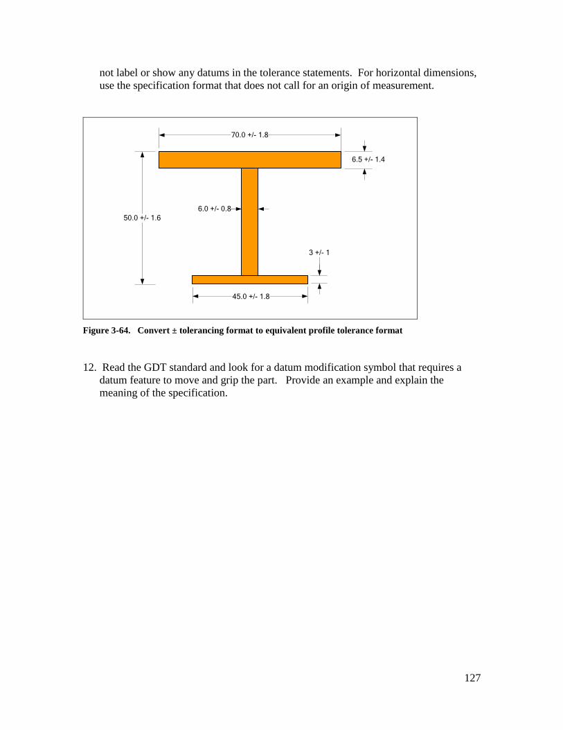
127

not label or show any datums in the tolerance statements. For horizontal dimensions,

use the specification format that does not call for an origin of measurement.

70.0 +/- 1.8

50.0 +/- 1.6

6.5 +/- 1.4

3 +/- 1

45.0 +/- 1.8

6.0 +/- 0.8

Figure 3-64. Convert ± tolerancing format to equivalent profile tolerance format

12. Read the GDT standard and look for a datum modification symbol that requires a

datum feature to move and grip the part. Provide an example and explain the

meaning of the specification.

128

Chapter-4 Default Tolerances

4.1. Overview

Default tolerances are tolerance statements that apply to a specific group or all geometric

aspects of a part that have not been explicitly toleranced. For example, if a hole size is

toleranced but its location is not toleranced, a default tolerance should apply to control

the location of the hole. Otherwise, the manufacturing personnel are not responsible for

the location of the hole even when the deviations well exceed manufacturing norms.

Default tolerances play an important role in assuring that every part is completely

toleranced before being sent to manufacturing.

When design engineers set up their drawings or CAD models for making prototypes, they

often specify the tolerances for just a few precision features. In such cases, designers

accept the outcome of the manufacturing process for non-precision features assuming that

reasonable care is exercised during manufacturing. While adherence to adequate

workmanship is expected from manufacturing personnel, having no verifiable

requirements on the geometry of features is risky and unacceptable for production

documentation used to produce thousands of parts. When tolerances are missing, the

designer has no legal grounds to dispute the manufacturing quality even when there are

gross mistakes in the part production. The use of default tolerances eliminates such risks.

Default tolerance statements are verifiable just like other tolerance statements. Default

tolerances, however, are only checked when there is an obvious mistake or lack of

expected workmanship in the part production.

In general, default tolerances help design engineers by reducing the time it takes to

explicitly tolerance every feature and by preventing inadvertent omissions. Every part

should have its own custom-made set of default tolerances. It is an unwise practice to

rely on company-wide policies, established default tolerances, historical records of

tolerancing similar parts, or any other guideline that absolves the designer from carefully

selecting the best default tolerances.

4.2. Default tolerancing methods

The common practice in default tolerancing is to place such tolerances in the title block

of drawings as ± limits on drawing dimensions and angles. The text “UNLESS

OTHERWISE SPECIFIED” or UOS appears along with the specification. A title block

tolerancing format similar to what is shown in Figure 4-1 is common.

129

Figure 4-1. An example of a typical title block default tolerances

Based on this default tolerance block, a dimension shown as 25 on a drawing would be

interpreted as 25 ± 1 mm while the same dimension shown as 25.00 is interpreted as 25 ±

0.25 mm. This scheme of default tolerancing has many drawbacks. For example, a

change of formatting from one CAD installation to another can completely change the

default tolerances. In addition, the dimensional tolerancing scheme is not feature-based

requiring the designer to pay attention to every dimension of the part. The main

objection to the use of default dimension limits is that it is incompatible with the

geometric tolerancing methodology in which the CAD model and part dimensions define

the theoretical or basic geometry of the part. For this reason, the use of default geometric

tolerances is preferred over default dimensional tolerances.

Any geometric tolerance statement can be used as a default tolerance. The most common

one is the profile of a surface tolerance that applies to all surface features of a part as

individual features or as any grouping of features. A default profile tolerance defines a

three-dimensional envelope around the entire part surfaces and thus controls every aspect

of the part geometry to the degree specified by the tolerance value. For example, a

default profile tolerance of 1.5 mm defines a theoretical gage as an envelope of thickness

1.5 mm around the basic geometry of the entire part as shown in Figure 4-2 for the

turning support part. The primary manufacturing process for this part is machining from

a plate and a 1.5 mm overall accuracy for the entire part is consistent with minimal level

of manufacturing workmanship.

130

Figure 4-2. Tolerance zone for profile of surface tolerance

The 1.5 mm zone is divided evenly about the basic geometry definition of all features. A

more suitable default profile tolerance would orient and locate the part features with

respect to a datum frame. Adding a datum frame calls for the part features to be more

accurately oriented and located with respect to the selected datum features. In the case of

the turning support, the bottom surface and the slot center plane define a suitable datum

frame. A default tolerancing scheme using this datum frame is shown in Figure 4-3.

131

Figure 4-3. Default profile of surface tolerance statement with datum references

In this example, untoleranced features are oriented and located with respect to datum-A

surface. The other locations (width-wise geometry) is controlled with respect to the plane

of symmetry of the slot or datum-B. The theoretical gage for this default tolerance

statement is shown in Figure 4-4. The theoretical profile, which is in the middle of the

tolerance zone, is not shown.

132

Figure 4-4. Theoretical gage for default profile of surface tolerance statement with datum

references

Default profile tolerances are preferred to have datum frames that fully fix the part to the

gage. The profile datum shown in Figure 4-4 leaves the part with one unfixed degree of

freedom relative to the datum frame. In order to completely fix this part we can select

one of the faces of the turning support as a tertiary datum-C and reference that datum in

the default profile tolerance as well. This is shown in Figure 4-5.

133

Figure 4-5. Default profile of surface tolerance statement with fully constraining datum references

In selecting the primary default datum feature, the design engineer must decide on the

best orienting feature of the part. Usually, the part’s mounting surface on the assembly is

a good primary orienting datum. The secondary and tertiary datums for default

tolerancing are usually the features that further locate and orient the part with respect to

the assembly.

4.3. Datum targets

The primary application of datum targets is to set up default tolerance datum frames for

parts that do not have precision surfaces. If we place a cast or forged part on any of its

surfaces, the part is likely to be unstable. Datum targets allow such surfaces to be used as

datums. Since the emphasis of this book is on machine design and machined parts, the

discussion of datum targets that follows is brief. Engineers who design cast parts should

become more familiar with various types of datum targets and their methods of

specification.

Consider the bottom surface of a cast part shown in Figure 4-6. Because of the bowed

shape, there is no repeatable way of aligning the planar datum simulator of a theoretical

gage with this datum feature. If we place this part on a flat table, it would rock with a

nudge.

134

Figure 4-6. A distorted surface would rock when placed on a flat surface

In Figure 4-6, we would like to define a datum simulator that can create a good physical

repeatable support for the part. A good way of supporting the part is to place the part on

three points which are as far apart as possible from each other, without being too close to

the corners and edges. The points must also be kept away from other surface anomalies

like parting lines or weld beads. This procedure is shown in Figure 4-7. The figure

shows two of the points in the front and a third point (with dashed lines) in the back.

Figure 4-7. Datum targets allow unique datum assignments on uneven surfaces

The design engineer can define the basic location of these target points using a datum

target symbol. Figure 4-8 shows an example.

135

A1 A2

A3

A3

A1

A2

Figure 4-8. The syntax for using datum targets to define the constraint geometry

The three points labeled A1, A2, and A3 define the datum-A plane. The basic distance

between the datum targets and their distances to the part edges is defined by theoretical

dimensions. Most CAD systems allow the designers to quickly insert datum targets. The

designers can also specify a variety of other target tip forms such as spherical tips,

cylindrical area tips, square area tips, edges, and even sliding datum targets. Any

arrangement of points, lines, or surfaces that constrain a part can be used as datum

targets. Sliding targets behave like expanding or contracting points or jaws with pointed

tips or edges that grab the part and constrain the part’s movements. By default, sliding

targets move in the direction normal to the surface on which they are defined but other

movement directions can be specified by notes.

For an example of using datum targets to define a datum frame for default tolerances

consider the familiar example of a plastic toy house shown in Figure 4-9.

136

Figure 4-9. A toy house

The primary orienting datum for this shape would be the bottom surface of the house.

We want all the surface features of this house to be more precisely oriented relative to the

bottom surface datum. Datum targets will be used to define the surface as the plastic

molded surfaces are uneven. To establish the primary datum, three datum target points

would be used. The datum simulator would consist of three pins on which the house rests

(datum plane-A). The targets defining the primary datum are shown in Figure 4-10 as

three arrows on the bottom surface. The arrow with the dashed outline is located near the

back wall. The datum targets and the resulting plane define the general level of the house

floor.

Figure 4-10. Defining datum targets and datum simulators

The secondary datum would locate all the features in widthwise direction. The secondary

datum simulator can be a pair of collapsing points gripping the house from the sides.

137

These targets define a center plane datum and are shown by two-sided arrows. The

tertiary datum can be a point in the center of the front or back wall. Once the house is set

up on the datum targets and immobilized, profile tolerance zones can be used to define

the extent of surface variation from the theoretical shape of the house. This profile

statement must have a value consistent with the tolerances that plastic molding practices

can easily hold when there are no errors in the process.

Default tolerances should be selected to best define the shape of a part and be insensitive

to local shape variations. This usually means placing the targets far apart on the most

prominent features of a part. Datum targets can also be used on machine parts for default

tolerance specification when the part's precision surfaces do not best represent the overall

shape of the part or are too small.

4.4. Default tolerancing and small features

One of the weaknesses of the default profile tolerancing is that a profile tolerance value

that is adequate for the entire part would usually not provide sufficient control for non-

precision small features such as small holes or bosses, grooves, fillets, webbings,

chamfers, ribs, etc. For example, if the 3-mm oil hole in the turning support part is left

without explicit tolerances, the profile default tolerance applies to it. For this small

feature, the default tolerance creates a relatively large acceptance zone as shown in

Figure 4-11. The 3-mm hole size can be as small as 1.5 mm or as large as 4.5 mm. It can

also be off center or tilted by several degrees. Even though this lubrication hole is not a

precision feature and may still function adequately, this amount of variation is usually

indicative of poor workmanship or other manufacturing problems.

Theoretical

LocationTolerance

Zone

4.5

1.5

Figure 4-11. Default profile tolerance zone for a small hole may not provide adequate control

To address the accuracy of small features the designer should consider tolerancing small

features directly rather than relying on the default tolerance. Explicit profile tolerances

should be added to control the sizes and, if necessary, the locations of small features.

138

Figure 4-12 shows the final specifications for the turning support part where the size of

the lubrication hole is controlled by a separate profile statement that calls for more size

precision while still consistent with minimal expected precision of manufacturing

practices. The location of the hole is left unspecified to be controlled by default

tolerances.

Figure 4-12. Small features may require explicit tolerance statements

This part would be fully defined when the design dimensions are imported into the

drawing. It is usually a good practice to place the dimensions and tolerances on two

separate layers such that each can be generated separately or together as in customary

production drawings.

4.5. Default tolerances for fillets and rounds

A part may have many fillets and rounds on many of its edges. Since these features are

usually small, default tolerance values for overall dimensions may even exceed the radii

of some fillets. These small features need to be controlled by narrower tolerances to

ensure their shapes are produced with reasonable accuracy expected from the intended

manufacturing process. One way of controlling such features is by one or more profile

statements applicable to identifiable features such as fillets and rounds. For example, a

default tolerance statement such as the one in Figure 4-13 may be appropriate.

139

Figure 4-13. Default tolerances including a statement for the size of small fillets and rounds

Small features such as small holes, webbings, chamfers, grooves, notches, or counter-

bored features may require similar tolerance statements either explicitly applied to the

features or as a default tolerance applied to named feature types.

Care must be exercised not to create a long list of default specifications. As a preferred

practice, default tolerance statements should be kept to a minimum. For example, a

default tolerance that applies to just one or two features is best applied directly to those

features. A manufacturing establishment would normally scan the default tolerances

ensuring that their processes are well capable of meeting them and afterwards the default

tolerances are ignored. Default tolerances that require levels of precision beyond just

basic workmanship should be avoided.

4.6. A different way of dealing with small features

Typical cast parts have a lot of small features and details and it is not always possible to

clearly name and identify their types on a model. Unless the default tolerancing scheme

can accommodate these small features, they would need to be directly toleranced. As a

result, the list of small features that need their own explicit tolerance statements on a

complex cast part can become extensive. An example of a cast part is shown in Figure 4-

14.

140

Figure 4-14. A cast part with many small non-precision features

We only needed one statement to require adequate workmanship for the larger-scale

features of the part. Ideally, we should need just one more statement to require adequate

workmanship to control the smaller-scale geometry of a part. This can be accomplished

with a special kind of profile statement. The needed profile tolerance statement must use

an adjustable tolerance value. The tolerance value becomes smaller as the feature

become smaller. For illustration, consider the geometry shown in Figure 4-15.

Ø5

2X Ø3

2.5

1.5

Ø4

Figure 4-15. A part with many small but non-precision features

141

This shape has a shallow slot, three small holes, a deep groove, and two small side

bosses. Assume that none of these features are precision but they are required to be made

with a minimum level of size accuracy expected from good workmanship using adequate

manufacturing processes. To meet the requirements, we can define a profile tolerance

with an adjustable tolerance value. The tolerance value would depend on the size of the

zone of inspection. The smaller the zone of inspection, the smaller the tolerance value

would become.

At first, the variable tolerance zone method appears to make things complicated both for

design engineers who specify them and for manufacturing personnel, who like to know

immediately if they can meet the minimal precision requirements. Fortunately, size-

adjustable tolerance values have been standardized and are known as the International

Tolerance grades or IT grades. We will cover the IT grades in more detail in Chapter-6.

A portion of the IT grades table is shown in Table 4-1 for illustration.

IT Grades

Feature Sizes IT 12 IT 13 IT 14 IT 15 IT 16 IT 17

0-3 0.10 0.14 0.25 0.40 0.60 1.0

3-6 0.12 0.18 0.30 0.48 0.75 1.2

6-10 0.15 0.22 0.36 0.58 0.90 1.5

10-18 0.18 0.27 0.43 0.70 1.10 1.8

18-30 0.21 0.33 0.52 0.84 1.30 2.1

30-50 0.25 0.39 0.62 1.00 1.60 2.5

50-80 0.30 0.46 0.74 1.20 1.90 3.0

90-120 0.35 0.54 0.87 1.40 2.20 3.5

120-180 0.40 0.63 1.00 1.60 2.5 4.0

Table 4-1. A portion of the table of International Tolerance Grades

Based on this table, a tolerance value of 0.4 mm applies to a 2 mm hole when the

tolerance grade of IT-15 is selected. The default tolerances for every process can be

associated with an IT grade. For example, a reasonable default tolerance grade for

general machining may range from IT-12 to IT-15 while a tolerance grade range for

various casting processes can be between IT-14 and IT-17. We can even use Table 4-1 to

come up with adequate values for the overall default tolerance as well. For example, the

largest dimension of the turning support part in Figure 4-12 is 130 mm. Selecting an IT-

15 grade for this part, for which the primary manufacturing process is machining, we can

select a tolerance value around 1.6 mm. In the case of the turning support a value of 1.5

mm was applied as the overall default tolerance.

In Figure 4-15, the sizes of small holes, the width of the deep groove, and the depth of the

slot are controlled by a 3 mm size zone of inspection. A profile tolerancing scheme for

controlling the size of small features of the part is shown in Figure 4-16.

142

UOS

25

Ø 5

B

C

IT 15 A B C

A

Figure 4-16. An example of a profile tolerance statement with an adjustable tolerance value

Based on this specification, the sizes of the 3-mm holes are controlled by a profile

tolerance with a tolerance value of 0.4 mm. The size of the deep groove and the depth of

the shallow slot are also controlled by a 0.4 mm tolerance zone. The size of the 5-mm

hole is controlled by a tolerance value of 0.48 mm. The distance between the two smaller

holes is controlled by an inspection zone that includes both features resulting in a profile

tolerance with a tolerance value of 0.84 mm.

A default tolerancing example for a die-cast gearbox housing

Figure 4-17 is a simplified model of a gearbox. The gearbox housing is made of die-cast

aluminum. It has many ribs and reinforcing features but except for a few surfaces that

require machining, the rest of its features are non-precision. Figure 4-18 shows the actual

assembly.

143

Figure 4-17. The simplified assembly model of a gearbox

Figure 4-18. Components of a gearbox

Figure 4-19 shows the surfaces of the gearbox housing that require precision

specification. These surfaces are highlighted in color.

144

Figure 4-19. Precision features of the gearbox housing

The highlighted flat surfaces, shown in red, are contact surfaces and must be machined

flat. The highlighted cylindrical surfaces, shown in blue, must be machined for fit of the

bearing outer diameters and for the fit of the endcap. The location of the tapped screw

holes must also be controlled with precision. Other surfaces are non-precision and are

left as-cast. The cast features can be controlled with default profile statements.

To define the profile statement necessary to control the large-scale geometry of the

gearbox housing we must define a suitable datum frame. Figure 4-20 shows the selection

of the default primary datum using three datum target points. The target points are

selected far apart to promote stability and insensitivity to local deformations. Notice that

the machined surfaces are not selected to define the primary datum; instead points on the

cast features are used. It is usually preferred to define the datum targets based on the

surfaces that represent the primary manufacturing process. The secondary and tertiary

datum targets are placed on the two edges of the part as shown.

145

Figure 4-20. Datum targets defining the primary datum

The default tolerance datum frame, along with the two profile statements shown on the

figure, complete the default tolerancing requirements of this part. The 2.5 mm profile

tolerance value is consistent with IT-16 grade for a part that has a largest overall

dimension in the range of between 120 and 140 mm.

Sometimes it is best to set up the default tolerances based on the precision of the

secondary process. Figure 4-21 shows the picture of the crankshaft of a small single-

cylinder engine. The primary manufacturing process is sand casting. The counterweights

are not precision features and remain as cast. The rest of the crank shaft surfaces are

turned to achieve the desired precisions.

146

Figure 4-21. The crank shaft of a single-cylinder engine

In this case, it is better to set up the default tolerances based on the secondary machining

process and explicitly tolerance the remaining cast features to have tolerances consistent

with the precision expected of sand casting process. Figure 4-22 shows a simplified

model of the crank shaft along with the default tolerance statements and explicit profile

tolerances for the cast portions of the crankshaft. The cast portions are shown in red.

There is no significance to labeling the datums by double letters such as AA, BB, or CC.

You may use such labeling schemes as visual aids to distinguish between datums

exclusively used for default tolerancing purposes versus other functional purposes.

147

Figure 4-22. The model of the crankshaft of a single-cylinder engine

The default profile tolerances control the machined features of the crankshaft while the

explicit profile tolerance statement applied to the cast part allows tolerance values larger

than that in the default statement.

Exercise Problems

1. Consider the gearbox housing cover shown in Figure 4-23. This aluminum die cast

part has many small features such as ribs, fillets, bosses, and holes.

148

Figure 4-23. The gearbox housing cover

Figure 4-24 shows a simplified model of the part in which a sample of non-precision

small ribs, holes, and bosses are shown.

Figure 4-24. Simplified model of the gearbox housing cover

149

Apply two default profile tolerance statements to control all non-precision aspects of this

part. The first statement is to control the large scale geometry of the part. The second

profile statement is to control the small feature sizes.

2. Add default tolerances to the drawing of the endcap part shown in Figure 1-32.

3. Add default tolerances to the drawing of the turning support part shown in Figure 1-

33.

4. Add default tolerances to the drawing of the transmission shaft part shown in Figure

1-34.

5. Add default tolerances to the drawing of the flange part shown in Figure 1-35.

150

Chapter-5 Tolerance Design for

Unconstrained Fits Between Two Parts Part-I

5.1. Overview

Unconstrained fits are the most critical and also the most precision fits in a machine

assembly. In an unconstrained fit, one part is sufficiently free to align or center itself

relative to a mating part. The most common unconstrained fits involve bearings. For

example, a ball bearing bore must typically have a tight fit with a rotating shaft. Size

precision, in the case of ball bearing fits, is so critical that often ground shafting must be

used. Another example of an unconstrained fit is the fit of a plain bearing to a bearing

housing. Such a fit must provide a light interference fit, which also requires precise size

control.

The size control of unconstrained fits is so critical and the tolerances are so small that a

standard has been developed just for the specification of precision sizes. This standard,

known as ANSI B4.2 Limits and Fits Standard, will be presented in the next chapter.

This chapter presents some of the concepts regarding fits that also apply to more general

cases of orientation-constrained fits and location-constrained fits to be presented in later

chapters. The application of the maximum material condition symbol m is also

presented in this chapter. In this and the next four chapters we will only discuss fits

between two parts. Fits involving multiple parts will be presented in Chapter-10.

5.2. Unconstrained fits versus constrained fits

Unconstrained fits between two parts occur when there are no constraining surfaces

limiting the orientation or the location of fitting features. In other words, one feature or

part is free to assume any position or orientation in space needed to align or center itself

with a mating feature. An example is the fit between the handle of a hammer and the

hammer head. A common engineering application of this kind of fit is between a bearing

bore and a shaft. This situation is shown in Figure 5-1.

151

Figure 5-1. An example of an unconstrained fit

The following applications usually require a precision unconstrained fit between the main

fitting features:

Rolling-element bearing bores and shafts

Rolling-element bearing outer races and housing holes

Plain bearings and shafts

Plain or flanged bearing outer diameters and housing holes

Gears and other shaft components (couplings, collars, pulleys) and shafts

Dowel pins and pin holes

Keys and keyways

Press fit or shrink fit features

In unconstrained fits, the fit tightness or looseness is usually of critical functional

importance and must be controlled with high precision.

Before exploring unconstrained fits, it is important to be able to recognize various

appearances of constrained fits. Constrained fits between two features also require the

features to fit together but in the case of constrained fits, the two features are required to

maintain a certain orientation, or position, with respect to each other. Figure 5-2 shows

an example of an orientation-constrained fit between two parts.

152

part1

part2

Constraint Surface

Figure 5-2. An example of an orientation-constrained fit between two features

In this example, the design intent is for the two features in part1 and part2 to fit together

while they are constrained to maintain a specific relative orientation. The relative

orientation is forced by the contact surfaces. If one or both fit features are not

perpendicular to their contact surfaces with sufficient accuracy, the features may not fit

together properly even though their sizes may allow free fit. Figure 5-3 shows another

constrained fit in which the features are not only orientation-constrained by the mounting

surfaces but also location-constrained by the locating edges.

part1

part2

Orienting Surface

Locating Surface

Figure 5-3. An example of an orientation and location constrained fit between two features

153

Another common location-constrained fit is the fit between two feature patterns or when

multiple features fit each other simultaneously. In a feature pattern, shown in Figure 5-4,

the fit features are constrained by each other and no single feature is completely free to

align itself independent of the other features. On part1, for example, the location of one

fit feature is constrained by another feature that fits simultaneously.

part1

part2

Figure 5-4. A feature pattern fit or simultaneous fit is always a constrained fit

In some situations, the constraint between two fit features is caused by a third part as


part1

part2

part3

Figure 5-5. A constrained fit between two features caused by a third part

The orientation and location relationship between part1 and part2 is constrained by part3.

Multipart fits will be discussed in Chpater-10.

154

The determination of whether a fit is unconstrained or constrained depends on how the

final assembly is going to force geometric relationships. Sometime the appearances may

be deceiving. An example of an unconstrained fit that looks like a constrained fit is the

light press fit of a flanged plain bearing into a housing bore as shown in Figure 5-6.

Flanged Plain

Bearing

Housing

Orienting

Feature

Figure 5-6. An unconstrained fit that appears like a constrained fit

This light press fit is an unconstrained fit as the bearing and bearing hole center

themselves freely for press-fit. When the bearing is pressed in, it stops when the flange

makes contact with the housing. Functionally there is no need for the planar surfaces to

align perfectly. Moreover, there are no design features, such as screws, that would force

the two surfaces to align. The fit features themselves orient the two parts with respect to

each other, not the contacting shoulders.

5.3. Fit assurance between two parts

To study the requirements of obtaining the minimum and the maximum looseness or play

in unconstrained fits, we can consider the simplest possible fit – the fit between a ring

and a bar. This fit is similar to the fit between a ring and a finger. The finger does not

need to be straight for the ring to fit properly provided the ring size is correct and it is not

too wide. This simplest fit situation is shown in Figure 5-7.

155

BarRing

Figure 5-7. Fit between a ring and a bar

To assure fit, the ring must be larger than the bar at each cross-section of the bar. The

design engineer can control the cross-sectional size of a feature through size limits or size

tolerance. For example, the size limits shown in Figure 5-8 assure a clearance fit.

24 - 25 23 – 24

Figure 5-8. Size limits assuring clearance fit

The minimum possible play in this fit corresponds to the largest (bulkiest) bar of cross-

section 24 mm, mating with the smallest ring of size 24 mm (also bulkiest). If a bar

happens to be manufactured at its bulkiest limit of size which corresponds to its

maximum size, it is said to be made at its maximum material condition or at MMC. The

special symbol m is used to indicate a feature at its maximum material condition. If the

bar is made at its skinniest limit of size which corresponds to its minimum size, it is said

to be made at its least material condition or at LMC. The special symbol l is used to

indicate a feature at its least material condition. In the example above, the size of the bar

156

at its MMC is 24 mm and the size of the bar at its LMC is 23 mm. For the hole feature

the situation is reversed; the smallest hole has the most material and its MMC size

corresponds to 24 mm. The LMC size of the hole corresponds to the largest hole size,

which is 25 mm.

In the case of the features in Figure 5-8, the minimum possible play is zero and occurs

when a 24 mm bar fits a 24 mm hole – both at their maximum material conditions. The

maximum possible play occurs when the two features are made at their LMC limits. In

this case the maximum play occurs when a 23 mm rod fits a 25 mm hole. The maximum

possible play is 2 mm.

In most practical unconstrained fits, the length of fit is longer than a thin ring and the

control of cross-sectional size alone is not sufficient to assure fit. Consider the example

in Figure 5-9.

Length-of-Fit

Figure 5-9. Cross-sectional size limits do not assure fit when the length-of-fit is long

The cross-sectional sizes of the two features are the same as the cross-sectional sizes of

the bar and the ring shown in Figure 5-7 but the two features no longer fit because the

ring is no longer thin. The length-of-fit is the length of the hole feature. The designer’s

problem is as before – how to assure fit with a desired minimum play while controlling

the maximum possible play from becoming excessive.

To assure a minimum play of Pmin between two mating features, the design engineer can

define two conceptual cylindrical surfaces, one for the shaft feature and one for the hole

feature. The size difference between the shaft and hole conceptual cylinders would be

Pmin as shown in Figure 5-10. In this case Pmin is 1 mm. These conceptual cylinders will

be called fit boundaries in this book. The fit boundary lengths of both features are equal

to the length-of-fit in this example.

157

Pmin =1

Hole Fit Boundary Shaft Fit Boundary25 24

50 50

Figure 5-10. Theoretical hole and shaft boundaries for mating features to ensure a 1 mm gap

To ensure a minimum play of at least Pmin = 1 mm between the two features after they fit

together, any length-of-fit portion of the shaft must fit inside the shaft fit boundary while

the hole must fit outside the hole fit boundary. Therefore, the designer should send the

following tolerancing instructions to manufacturing:

Make the shaft feature such that every 50-mm length of it would fit inside a

cylindrical zone of size 24 mm, and make the hole feature such that it would fit

outside a cylindrical zone of size 25 mm.

If manufacturing carries out the production according to instructions, the design objective

is achieved. Figure 5-11 shows one example of two actual features that fit together and

have a minimum play of a little more than 1 mm after assembly.

Pmin

Hole Fit Boundary2524Shaft Fit Boundary

Figure 5-11. An example of two features conforming to their fit boundary requirements

158

Fit boundaries are known as virtual boundaries in the GDT standard. Fit boundaries are

theoretically perfect cylinders for cylindrical features, or a pair of parallel-planes for

width features. It should be clear that the fit boundary controls the combined effect of

cross-sectional size and feature axis straightness. For the shaft, the combination of the

cross-sectional size and axis bending must be less than 24 mm. Similarly for the hole, the

combination of cross-section size and axis bending must leave an opening larger than 25

mm. For the fit of width features, the center plane flatness must be used instead of the

axis straightness.

The question is how the design engineer should efficiently communicate the fit boundary

requirement to the manufacturing and inspection personnel. For someone who does not

know the GDT symbols, the following tolerance statement note captures the fit boundary

requirement for the shaft and communicates the functional needs of the design:

Make the shaft such that it would fit inside a 24-mm hole.

This instruction is fine for inspection personnel as the final product is available and can

be checked against a gage the size of the fit boundary. During manufacturing, however,

the given instruction is difficult to use. An alternative form in terms of feature cross-

sectional sizes and bending of axis is more helpful in manufacturing because these

deviations can be quantitatively measured separately. We can use the following

equivalent description of the fit boundary:

Make the shaft such that its maximum cross-sectional size would not exceed 24

mm. If the cross-sectional size is 24-mm, the feature must be perfectly straight.

When the cross-sectional size is smaller than 24-mm, the shaft can bend by the

difference between the actual size and the MMC size of 24 mm.

For example, the axis of a 23 mm shaft can bend 1 mm and still fit the 24 mm boundary.

Even a 20 mm shaft can bend 4 mm and still pass the tolerance statement. Obviously, the

above tolerance statement sets no limit on how small the shaft diameter can be. Another

statement would be required to limit the maximum fit play by excluding shafts that are

too small.

Specifying the LMC size is the proper method of controlling the minimum shaft size and

the resulting maximum fit play. For example, we can use 23-mm for the smallest

acceptable size of the shaft (or its LMC size). Adding this minimum size limit and also

abbreviating the text of the previous instruction, the new tolerance requirement should

have the following two parts:

Make the shaft such that its cross-sectional size is between 23 and 24 mm

If the cross-sectional size is 24-mm (at MMC), the shaft must be perfectly straight.

The two statements imply that what is required is a fit boundary size of 24 mm and the

minimum cross-sectional size is to be 23 mm. Two extreme shapes of the shaft that

159

would be acceptable based on the tolerance description above are shown in Figure 5-12.

The fit boundary for the shaft simply acts like a tube – any shape that fits inside the tube

passes the fit boundary requirement.

24 24

23

1

Figure 5-12. Acceptable feature at MMC (left) and at LMC (right) with maximum bending

The design engineer must now translate the tolerance requirements stated above in text

form into GDT standard symbols and place those symbols on the drawing. Figure 5-13

shows the way it must be indicated on the drawing.

Ø 0 M

Ø 23-24

Figure 5-13. Defining a 24 mm fit boundary using the GDT standard format

The geometric tolerance statement indicates that if the feature is made at its maximum

material condition of 24 mm, then it has to be perfectly straight. The fit boundary of the

shaft in this case is equal to its MMC size. If appropriate, we can make the fit boundary

larger than the MMC size of the shaft by using a non-zero straightness for tolerance

160

value. For example, to define a 25 mm fit boundary for a shaft with 23-24 mm size

limits, we must specify a 1 mm straightness tolerance at MMC as shown in Figure 5-14.

Ø 1 M

Ø 23-24Fit Boundary 25 mm


In this case, a 24-mm shaft is allowed to bend 1 mm while a 23-mm shaft can bend 2

mm.

5.4. Theoretical gages for tolerance statements that use the m symbol

For tolerance statements that use m next to the tolerance value, the theoretical gage has

the size and shape of the fit boundary defined by the tolerance statement. For a shaft, the

acceptance zone is defined as a tube, and for a hole, the acceptance zone is defined as a

bar. Figure 5-15 shows the theoretical gage for the tolerance specification in Figure 5-13

where the MMC size is 24 mm and straightness tolerance is zero at MMC. The tube

gage must be at least the length of the bar.

161

Ø 24

Figure 5-15. Theoretical gage for straightness specification of Figure 5-13

This theoretical gage can be physically made as a tube and physical gaging amounts to

checking to determine if the manufactured bar fits inside the tube. This kind of physical

gaging is feasible with all tolerance statements that use m because all m related

specifications are about feature fit and fits are easy to test physically.

5.5. Fit formula

We can summarize the requirements for a clearance fit as a formula and also develop a

formula for the maximum possible play in a fit. The following nomenclature will be used

throughout the rest of this book. Size in the following statements refers to a diameter or a

width dimension.

FBH: The size of the fit boundary of an internal feature (a hole or a slot)

FBF: The size of the fit boundary of an external feature (a shaft or a rail)

Hmin: The MMC size of a hole or slot feature (minimum size)

Fmax: The MMC size of a shaft or a rail feature (maximum size).

Hmax: The LMC size of a hole or slot feature (maximum size)

Fmin: The LMC size of a shaft or a rail feature (minimum size)

TH, TF: The specified geometric tolerance values at MMC for hole and shaft

features

tH, tF : The size tolerance values for hole and shaft features. The size tolerance is

the total tolerance range on a size dimension (difference between MMC and LMC

dimensions)

Pmax: The maximum possible play in clearance fits

Pmin: The minimum assured play in clearance fits

162

To develop the Pmin and Pmax formulas for a fit, consider the hole and shaft fit boundaries

in Figure 5-16.

Pmin=1

Hole BoundaryShaft Boundary

FBH FBF

Figure 5-16. The difference in fit boundaries defines the minimum assured play

The minimum assured play in a clearance fit is the difference between the two feature’s

fit boundaries

Pmin = FBH – FBF [1]

Defining the fit boundaries in terms of MMC size and geometric tolerances

Pmin = (Hmin – TH) – (Fmax+TF) [2]

Or

Pmin = (Hmin – Fmax) – (TH + TF) [3]

Eq.[3] is the minimum play formula for a clearance fit. Once the tolerance values are

specified, we can set up (Hmin – Fmax) to be equal to the sum of tolerances (TH + TF) for a

zero clearance fit. Setting the minimum play to zero would set the sizes of the fit

boundaries equal to each other. Setting Pmin ≥ 0 and solving for the geometric

tolerances, we get

(Hmin – TH) – (Fmax+TF) ≥ 0 [4]

Or

TH + TF ≤ Hmin – Fmax [5]

Eq. [5] indicates the condition for a clearance fit and is called the fit formula.

The maximum play in a clearance fit occurs when the two fit features are made at their

least material condition and are perfectly straight. The maximum play formula based on

LMC sizes is

Pmax = Hmax – Fmin [6]

where Hmax and Fmin are the LMC hole and shaft feature sizes. Eq.[6] is the maximum

play formula. By substituting Hmax = Hmin + tH and Fmin =Fmax – tF into Eq.[6] and

163

considering Eq.[3], we can write Eq.[6] in terms of tolerances of size and geometric

tolerances as

Pmax = tH + tF + TH + TF + Pmin [7]

The maximum possible play is the sum of all tolerances (geometric and size) plus any

assured minimum play in the fit. If the tolerances are set up for a fit with a minimum

play of zero, then the maximum play is just the sum of all tolerance values.

Example-1

The MMC sizes of a hole and shaft are Hmin=12 mm and Fmax=10 mm respectively.

Straightness tolerance values are specified at MMC.

a) Determine the geometric tolerances that assure a fit with a minimum play of zero.

What are the sizes of the fit boundaries?

b) Determine the geometric tolerances to have a fit with a minimum assured play of

1 mm. What are the sizes of the fit boundaries?

c) Determine the maximum possible play in the fit for case (b) when size tolerances

are 0.5 mm (Hmax=12.5 mm and Fmin=9.5 mm).

Part-a) Using the fit formula,

TH + TF ≤ Hmin – Fmax

or

TH + TF ≤ 12– 10 = 2 mm

If the geometric tolerances (straightness specifications) are selected to be equal (TH = TF)

then we must have

TF = TH ≤ 1 mm

The straightness tolerance values define the size of the fit boundary for the shaft to be

equal to 10+1=11 mm. The fit boundary of the hole is also 12– 1=11 mm, guaranteeing a

clearance fit with a minimum play of zero.

Part b) In order to have at least a minimum play of Pmin in the clearance fit, we must add

a Pmin to the hole fit boundary, or subtract a Pmin from the shaft fit boundary. The

resulting tolerance relationship to assure a minimum play of Pmin is

TH + TF ≤ Hmin – Fmax – PminFor Hmin=12, Fmax=10, and a Pmin of 1 mm, we must have

TH + TF ≤ 1

If the geometric tolerances are selected to be equal (TH = TF) then we must have

TH ≤ 0.5 mm

TF ≤ 0.5 mm

These straightness tolerance values define the size of the fit boundary for the shaft to be

equal to 10+0.5=10.5 mm. The fit boundary of the hole is 12– 0.5=11.5 mm

guaranteeing at least a 1 mm clearance fit.

Part-c) The maximum possible play for the case (b) solution can be as large as

Pmax = Hmax – Fmin = 3 mm

Using the tolerance values formulation, we get the same result

164

Pmax = tH + tF + TH + TF + Pmin

Pmax = 0.5 + 0.5 + 0.5 + 0.5 + 1 = 3 mm

In most unconstrained fits such as fit of bearings or gear hubs etc., the minimum and

maximum plays and interferences are both critical to the proper function of the fit. For

constrained fits it is usually best to set Pmin=0. This choice assures free assembly and

results in the smallest play in the fit.

5.6. Default form control implied by limits of size

In the GDT standard, there is more geometry control behind the limits of size than just

the control of cross-sectional size limits. In the absence of other specifications the limits

of size for regular features-of-size also control the form of such features. The default

form control that automatically applies to a cylindrical feature is a zero straightness

tolerance at MMC. For example, when a shaft with size limits of 23-24 mm is indicated

on a drawing without any explicit straightness specification, the feature is also required to

have a 24-mm fit boundary. Figure 5-17 shows the implied meaning of this default

requirement.

Ø 0 M

Ø 23-24Ø 23-24

This Means This

Figure 5-17. The default form control of GDT standard

The default form control of the GDT standard is known as Rule#1. To override Rule#1, a

straightness tolerance can be explicitly applied to the feature with a desired tolerance

value. When form control is not needed at all, the independency symbol can be used with

the size limits as shown in Figure 5-18.

165

Ø 23-24 I

Figure 5-18. The use of independency symbol

The application of the independency symbol will be presented later in an example.

5.7. Use of zero geometric tolerance at MMC

Fit boundaries are defined by adding or subtracting a geometric tolerance to the MMC

size of a feature. In unconstrained fits, the geometric tolerance is axis straightness for

cylindrical features and center plane flatness for width features. There is an unlimited

combination of MMC sizes and geometric tolerances that can define the same fit

boundary, including the use of zero geometric tolerance at MMC. What factors should be

considered in determining the best choice of tolerance statements? Consider an example

that compares the use of zero geometric tolerance at MMC with an alternate that allows 1

mm geometric form tolerance at MMC. Figure 5-19 shows two examples that define the

same fit boundary. The combined tolerances of size and straightness in both cases is 2

mm.

Ø 1 M

Ø 22-23Ø 22-24

Ø 0 M

(a) (b)

Figure 5-19. The tolerance statements define the same fit boundary for the feature

166

Both of these options define a fit boundary of 24mm. In addition, both specifications

have a LMC size of 22 mm and therefore the maximum possible play resulting from their

use in an unconstrained fit is also the same. In other words, the features that are made

based on the two specifications allow the same performance in terms of fit and play in a

two-part assembly.

There is, however, an important difference between the two options even for fit purposes.

While size tolerance can convert into additional geometric tolerance, the GDT standard

does not allow geometric tolerances to convert into additional size tolerances. Consider

an actual feature with a cross-sectional size of 23.5 mm and an actual bend of 0.4 mm.

The feature would fit into the 24 mm fit boundary and should be acceptable for fit. The

specification (a) in Figure 5-19 accepts such a part but the specification (b) rejects the

part because it exceeds the 23 mm size limit. In the above example, when the part is

made to be very straight, the 1 mm allowance for straightness is not permitted to be used

to widen the size limit on the MMC side. For fit purposes, the zero tolerance straightness

option makes the variations in size and straightness interchangeable both ways. An

actual feature made close to its LMC limit of size leaves maximum allowance for

bending. Conversely, a feature made with very little bending leaves maximum allowance

for size.

Applying zero tolerance at MMC is also the easiest way of indicating the fit boundary

requirement as the size of the fit boundary would correspond to the specified MMC size

of the feature. Zero geometric tolerances allow the design engineers to combine the size

and geometric tolerance into one tolerance – a combined size tolerance. The difference

between the LMC and MMC size limits becomes the sum of size and geometric

tolerances applied to the feature. This provides the maximum flexibility to the

manufacturing to meet the tolerance needs at minimum cost. When the manufacturing

sees the wide 22-24 mm tolerance of size, they can select the best process to obtain an

acceptable feature. For example, if they have a process that can hold size tolerances

very well but not the bending tolerances, they can target a size just above the LMC of 22

mm. This gives them almost 2 mm of bending allowance. On the other hand, they may

have a process that does not hold size tolerances very well but is accurate in keeping the

feature straight. In such a case, manufacturing can target the middle of the tolerance

range, such as a 23 mm size, to have maximum size allowance. The result of the above

reasoning is that, whenever possible, it is best to specify zero geometric tolerance at

MMC for unconstrained fit purposes. A zero straightness tolerance at MMC is often

implied with standard parts. For example, a standard dowel pin with a declared

maximum size of 10 mm is implied to have a 10 mm fit boundary and fit entirely inside a

10 mm hole.

The only potential drawback of zero geometric tolerances is that the features appear to be

specified to have zero geometric tolerance, or perfect form. A zero-tolerance value is

perceived as impossible by some manufacturing personnel. This can become a source of

potential confusion. Well-trained manufacturing personnel, however, know that zero-

tolerance specifications give them the most flexibility and control. Trained

manufacturing personnel understand that the size limits are in fact a combined tolerance

167

of size and geometric tolerance. The manufacturing personnel know that they are free to

divide up the combined tolerance between size and straightness any way they deem

advantageous as long as the fit boundary requirement is met. If the use of zero geometric

tolerance proves to be awkward in a production environment, the design engineer should

specify a non-zero tolerance. Zero geometric tolerance can only be used when m or l

symbols are used in the tolerance statement.

5.8. Fit formula when using zero geometric tolerancing at MMC

Using zero geometric tolerance method simplifies the fit formula by including the

geometric tolerance into the size limits. We can write the fit formula


in the following form:

(Hmin – TH) – (Fmax+TF) ≤ 0

Interpreting each term as a new limit of size and using new symbols for the two terms in

parentheses, the fit formula becomes

H0min – F0max ≥ 0

where H0min is the MMC size of the hole feature when zero geometric tolerance is used.

Similarly, F0max is the MMC size of the shaft feature when zero geometric tolerance is

used.

To convert a specification with non-zero geometric tolerance at m to one with zero

geometric tolerances at m, we must expand the size limits by the value of the geometric

tolerance on the MMC side. For example, if the hole size limits are 20-21 mm and the

selected geometric tolerance is 0.5 mm, the equivalent size limits for zero geometric

tolerance becomes 19.5-21.0 mm. We simply expand the hole size limits of 20-21mm on

the MMC side of Hmin=20 mm by TH=0.5 mm to get H0min = 19.5 mm. For a shaft feature

of limits 19-20 mm with a specified geometric tolerance of 0.5 mm at MMC, the size

limits for zero geometric tolerance becomes 19.0-20.5 mm. Again, we expand the size

limits of 19-20 mm on the MMC side of Fmax=20 mm by TH=0.5 mm to get F0max = 20.5

mm. F0max and H0min also define the sizes of fit boundaries and gages for the pin and hole

features.

5.9. Defining a fit boundary without the m modifier

Fit boundaries can be defined indirectly with straightness tolerances that do not specify a

modifier. This practice is necessary in cases where the feature size is to be precisely

controlled for a different functional reason. Straightness tolerance statements without a

modifier are said to be regardless of feature size (RFS). Figure 5-20 shows an example

of two specifications with equal fit boundaries. The left side statement uses the usual m

modifier and the right side statement uses the specification without a modifier. The fit

boundaries of the shaft for MMC or RFS specifications are both 24 mm. The fit

boundaries of the hole for MMC or RFS specifications are also both 24 mm. Note that

unlike the m-modified statement we cannot inspect the RFS tolerance statement by a fit

test inside the fit boundary. The RFS statement is a direct axis control statement. The fit

168

boundary is just an indirect consequence of not allowing a 23 mm feature bend more than

1 mm.

Ø 1

Ø 22-23Ø 22-23

Ø 1 M

Ø 25-26

Ø 1 M

FB = 23 +1 = 24 FB = 23 +1 = 24

FB = 25 - 1 = 24

Ø 25-26

Ø 1

FB = 25 - 1 = 24

Figure 5-20. Comparing m modified and RFS specifications

Since the fit boundary sizes and LMC sizes are the same for MMC or RFS specifications,

the two set of specifications perform the same in a fit. The two schemes both assure fit

and can lead to the same maximum play. The m-modified statement is better because it

adds manufacturing flexibility. The m-modified statement allows the straightness to be

up to 2 mm for a pin made close to its LMC size while the RFS statement allows only 1

mm regardless of the pin size.

5.10. A note on the use of modifiers

When applicable, the proper use of tolerance modifiers provide additional manufacturing

advantages by allowing a combined tolerance to be allocated as needed. This can lead to

a wider tolerance range where it is most needed. The manufacturing and inspection

departments refer to this additional possible tolerance as bonus tolerance. Not using a

169

modifier, however, does not make the tolerance specification wrong – it simply would

not allow this possible bonus tolerance. Even using the opposite modifier to what is

appropriate does not make the tolerancing scheme wrong. What makes the tolerancing

scheme wrong is missing specifications or tolerance values that are not correctly

specified to assure fit. The use of a modifier, when appropriate, simply makes the

tolerance specification better. The m modifier is the preferred choice for two-part fits.

Whatever specification is used, care must be exercised to make sure that fit is possible in

all situations allowed by the specified tolerances.

5.11. Unconstrained fits and Rule#1

In most applications of unconstrained fits such as fit of bearings, gears, press-fits, dowel

pins, or various shaft-hub fits, the use of default straightness control (Rule#1) is

appropriate. In these applications the length of fit is short (compared to the fit diameter)

and the use of size limits alone, which imply zero straightness tolerance at MMC, is

usually a good choice.

There is a common unconstrained fit application, however, in which the default

straightness control should be removed for one of the mating features. When a bearing

slides on a long rod as shown in Figure 5-21, the length of fit is short but moves along the

length of the rod defining a moving fit window. A similar situation occurs when a dowel

pin fits a shallow hole.

10

200

Figure 5-21. A sliding fit with a short length of overlap

The rod’s straightness for fit purposes is only needed over 10 mm lengths of the rod to

achieve proper fit in sliding. If only size limits are applied to this long rod, the size limits

imply perfect straightness at MMC for the entire length of the rod. In this example, if we

use more realistic numbers for a rod sliding on a bearing, the recommended sliding fit

dimensions would be 5.000 – 5.012 mm for the bearing hole and 4.998 – 4.986 mm for

170

the bar. These dimensions are indicated in Figure 5-22 along with the default

straightness control they imply.

Ø M0

4.998 – 4.986

10

5.000 – 5.012

Ø M0

Figure 5-22. Sliding fit dimensions along with their default form control

The default control limits are adequate for the bearing hole but the bar default control

requires the entire length of the bar to be straight with much higher precision than

needed. In this example, the rod can be out of straight by only 0.012 mm over its entire

length even when its cross-section is at LMC size of 4.986 mm. It is very costly to make

a rod this straight over a long length and, more importantly, this level of straightness

precision is not needed for proper fit and sliding action of the mechanism. The correct

specification should only require zero tolerance at MMC over all 10 mm lengths of the

bar. Figure 5-23 indicates how to apply this specification.

Ø M0/10

4.998 – 4.986

10

5.000 – 5.012

Figure 5-23. Proper specification type when a bearing slides on a rod

171

Note that this specification allows a smooth sliding fit but does not place a direct limit on

the total bending of the bar. An additional straightness control specification should be

added to limit the total bending of the entire bar. To place an additional constraint to

limit the total amount of rod bending, the specification format shown in Figure 5-24 can

be used.

Ø M0/10

4.998 – 4.986

Ø 0.1

Figure 5-24. The upper specification assures sliding fit while the lower specification directly controls

the overall bending of the bar

Even if the original per length statement may control the total bending of the rod to be

less than the overall total bending specification, it is important to apply an additional

straightness limit. The reason is that the direct specification of the total straightness

control leaves no doubt as to what is required. This is the better strategy to communicate

design intent to other designers. In this case the design intent is well communicated to

whoever is going to read the print. The intent is that there is a precise sliding fit on this

bar over a bearing length of 10 mm, and the overall bar is to be straight for other

functional reasons.

5.12. Unconstrained interference fits

The fit formula presented earlier applies to clearance fits where the features are intended

to be assembled without force. In all situations where random assembly is required, the

fit boundary of the shaft (external) feature must be specified to be smaller than or equal to

the fit boundary of the hole (internal feature). If there is an overlap between the fit

boundaries, there is a risk of features not assembling freely. In all intentional interference

fits, however, the interference is functionally important and the designer wants to have a

guaranteed minimum interference. Interference fits are always unconstrained fits. The

maximum interference is dictated by the MMC sizes of the fitting features. The

minimum interferences occur when features are at their LMC states.

In Figure 5-25, the minimum assured interference is 0.1 mm when both features are at

LMC, and the maximum interference is 0.3 mm when both features are at MMC. For

172

metallic parts these interferences are very large and unattainable; the larger numbers are

used here to convey the concepts. More realistic interference values will be presented in

the next chapter where the standards of limits and fits are introduced.

Hole Shaft

24.124.324.2

24

Figure 5-25. An example of interference fit

For interference fits, the same fit formulas apply except that play values become

negative. In the following formula, Pmin represents the maximum interference.

Pmin = Hmin – Fmax

And Pmax represents the minimum interference of

Pmax = Hmax – Fmin

Note that these formulas ignore the possible contribution of straightness tolerance to the

resulting interferences. The reason is that in interference fits the shaft is guided through

the hole by force. Only the cross-section sizes are important. Even if the shaft is not

straight, it would deform elastically (or plastically) to take the shape of the hole.

Exercise Problems

1. Consider the pin shown in Figure 5-26.

173

Ø 0.5 M

Ø 14 - 15

Figure 5-26. A pin with size and straightness tolerance specifications

Determine:

a) The MMC and LMC sizes of the shaft

b) The size of the shaft’s fit boundary

c) The amount of bending allowed when the feature is 14.6 mm

d) The equivalent size limits for fit when the straightness tolerance is zero

2. Consider the hole feature shown in Figure 5-27.

Ø0.5 M

Ø 16-17

Figure 5-27. A hole feature with size and straightness tolerance

Determine:

a) The MMC and LMC sizes of the hole

b) The size of the hole’s fit boundary

c) The amount of bending allowed when the feature is made at 16.3 mm

d) The equivalent size limits for fit when the straightness tolerance is zero

e) When this part is fit to the shaft in Problem-1, what is the minimum and

maximum possible play in the fit

3. A rectangular key is to fit a keyway as shown in Figure 5-28. The key is desired to

have an unconstrained fit to the keyway.

174

Ø 0.05 M

Ø 0.05 M

5.05 – 5.12

4.90 – 4.95

Figure 5-28. Fit of a key and a keyway

The fit tolerances are specified as shown in the figure. Determine:

a) The MMC and LMC sizes of the key and keyway

b) The size of the key and keyway fit boundaries

c) The amount of center plane bending allowed when the key is made at 4.95 mm

d) The amount of center plane bending allowed when the keyway is made at 5.05

mm

e) The equivalent size limits for key and keyway when the flatness tolerances are

converted to zero value at MMC

f) When the key and the keyway fit, what is the minimum and maximum possible

play in the fit

4. An off-the-shelf ground steel shafting has a nominal diameter of 8 mm and a size

tolerance of (-0.005,+0). The manufacturer indicates that the shaft straightness is

held to within 0.0003 mm/mm.

Determine:

a. The MMC and LMC sizes of the shaft

b. The fit boundary associated with a 10 mm length of the shaft

c. The maximum out of straightness that may result for a 100 mm length of the

shaft

175

Figure 5-29 shows how out-of-straightness increases with the length of the shaft for a

constant per unit length straightness.

Out of Straightness

Figure 5-29. The out-of-straightness accumulates rapidly with feature length

Hint for part (c): An approximate formula for obtaining the maximum out-of-straightness

of any length of a shaft given per unit length bending of a shaft is

lL tl

Lt

2

2

In this formula, tl is the straightness over a given length of a shaft l. The resulting

straightness over a length L of the shaft is tL. In this problem l=1 mm, tl = 0.0003 mm,

and L=100 mm for the last question.

176

Chapter 6 Tolerance Design for

Unconstrained Fits Between Two Parts Part-II

6.1. Overview

The previous chapter introduced the general concepts regarding unconstrained fits.

Arbitrary size limits and large straightness or flatness tolerance values were used to better

convey the concepts. In practice, the designer should exercise great care in the selection

of size tolerance values in unconstrained fits because the fit plays (or interferences) are

critical for proper function of precision joints. For precision bearing fits and other

unconstrained fits size tolerances are very small. Slight deviations from what works can

easily lead to non-functioning fits or excessive and unnecessary manufacturing costs.

This chapter presents the necessary guidelines that can help design engineers to quickly

select the correct size limits for precision fit applications in machine design and assure

proper function while using the most economical tolerances.

Figure 6-1 shows an extension shaft that fits over a drive shaft and extends it. A gear is

mounted at the free end of the extension shaft and is used to drive a gearbox, which is not

shown. The extension shaft is shown in transparent display state to show the drive shaft.

Figure 6-1. Extension shaft assembly

177

Figure 6-2 shows the features and precision fits associated with the extension shaft. The

designer must carefully specify the size limits of the features shown in the figure.

Figure 6-2. Critical fits associated with the extension shaft

Determining the correct size limits that work properly for the gear fit, the bearing fit, the

Woodruff key fit, the spring pin fit, and the drive shaft fit is not easy without helpful

design guidelines. Relying on guesswork for the size limits of such fits almost always

leads to inferior selections. Using the information in this chapter allows a designer to

quickly specify the correct and most economical size limits for a variety of unconstrained

fits. The end result would be size specifications in either a coded format or as numerical

limits (or both) as shown in Figure 6-3 for the extension shaft.

178

Figure 6-3. Precision size limits specified for an extension shaft

The tolerancing of this extension shaft will be discussed again at the end of this chapter to

illustrate the solution details.

The standard of limits and fits, ANSI B4.2, defines a list of size limits in coded format.

The coded format includes both letters and numbers. For example, the code 25f7 is

equivalent to size limits of 24.980 – 24.959 mm. The advantage of having coded size

limits is that manufacturers of standard parts, such as bearings and gears, can express the

tolerances associated with their products in coded form. This eliminates the possibility of

error and allows quick communication of part precisions. Manufacturers can also

recommend mating part tolerances that fit their parts in coded format. Another advantage

of coded limits is that it allows design engineers to quickly determine adequate size limits

for a variety of common applications.

6.2. An overview of the limits and fits standard (ANSI B4.2)

A general understanding of how coded size limits convert into numerical limits is helpful

in selecting the best size limits for fitting components. Coded size limits are made up of

three designators. The first designator is the basic or theoretical size. For example, in the

code 25f7 for a shaft feature, the number 25 is the basic size. In a fit, the basic size

should be the same for both the hole and the shaft. The second designator is a letter that

indicates an offset or basic size modifier. In 25f7, the letter f is an offset designator. The

offset values can be looked up in the tables in the standard and in the case of f offset, the

value is -0.02 mm. The offset modifies the basic size of the shaft from 25 mm to an

offset size of 24.98 mm.

The offset size indicates one of the size limits. The offset size is usually the desired size

if manufacturing could produce the part with exact precision. The other size limit is

179

determined by adding or subtracting a size tolerance value. The third designator is an

index number representing a tolerance value. In the case of 25f7 the tolerance index is 7

leading to a tolerance value of 0.021 mm when looked up in the International Tolerance

Grade table. The two limits 25f7 and 25f16 both indicate a desired 24.98 mm size but the

25f7 allows little deviation from that desired size while 25f16 allows a lot. The main cost

of creating a feature within size limits is associated with the tolerance index. Figure 6-4

shows the conversion of the limit codes to actual size limits for the 25f7 specification. In

this case, the offset size is the largest limit of size and the tolerance value subtracts from

the offset size to define the other limit.

Shaft 25

25f 25f7

Basic Size Offset Size Size limits

24.98024.959

24.980

Figure 6-4. Conversion of size limit codes to actual size limits

Most CAD systems allow a design engineer to select size limits based on limits and fits

coded format. The selections are then automatically converted to size limits and placed

on the model drawings if desired. The narrow size limits in this example are typical of

size limits necessary to achieve bearing fits or other precision fits in machine design. In

the case of 25f7, the total size tolerance is 0.021 mm. For comparison, the thickness of

regular household aluminum foil is 0.024 mm.

Fit is a relationship between two mating features and is characterized by extreme limits of

looseness or tightness. The loosest fit occurs when the largest holes (within its limits of

size) fit the smallest shafts, i.e. both features are at their least material state. The tightest

fit occurs when the smallest holes fit the largest shafts, i.e. both features are at their

maximum material state. The following sections present the information necessary to

guide the design process in selecting proper size limits for common precision fits. Before

reading the rest of this chapter you can try the LAF Excel program that converts any

coded size limits to numerical limits. The program can be downloaded from the book

web site. The program also finds the extreme fit values for any combination of holes and

shafts. After running the LAF program and invoking the associated macro, you should

see the following dialog window.

180

The yellow boxes on the left side are to input coded size information about holes. In this

case, the user has selected 25 mm basic size, an offset code of H, and a tolerance grade of

8. The corresponding numerical hole limits are calculated to be between 25.000 and

25.033 mm leading to a size tolerance of 0.033 mm. The green boxes on the right side

are to input information about shafts. In this case the basic size is also 25 mm, the offset

code is f and the tolerance grade is 7. The corresponding size limits for the shaft are

calculated to be between 24.959 and 24.980 mm with a size tolerance of 0.021 mm. The

blue box on the bottom of the screen indicates the extreme fit values, which in this case,

is a clearance of 0.020 mm for the tightest fit and a clearance of 0.074 mm for the loosest

fit.

6.3. Preferred sizes

When selecting basic sizes for unconstrained fits, the designer should give preference to

sizes that are likely to have available off-the-shelf tooling or components. For example,

there is a good chance of finding 10 mm drills, 10 mm ground shafting, or 10 mm bore

size bearings. It is unlikely to find any tooling or components at odd sizes. For economic

reasons, the best choices for precision fit applications are the sizes that the ANSI B4.2

standard has defined as preferred basic sizes. When having a choice, selection from these

181

preferred sizes often leads to lower production costs. Off-the-shelf parts and tooling are

often made at other standard sizes as well. For example, drills and reamers are made at

finer size steps than the standard preferred sizes. When selecting basic sizes for holes

intended to be drilled or reamed, selection from the list of widely available tool sizes is as

good as selection from the list of standard preferred sizes. The list of the preferred first

choice and second choice sizes can be seen in the choices for basic size specification in

the LAF program.

6.4. Offsets letters (fundamental deviations indicator letters)

Offset values designated by letters modify a feature’s basic size for the application.

Offsets directly relate to the function of the fit as they dictate the desired tightness or

looseness of the fit. We can think of offset sizes as the exact sizes needed for application.

By changing the offset letters the designer influences the characteristics of the fit. Offset

designators use lowercase letters for shafts and uppercase letters for holes. Offset

designator letters from a to h are negative and reduce the basic size of a shaft and are

usually intended for clearance fits. The offset value for h is zero. For example, the offset

size of a 25h9 shaft is 25 mm. Figure 6-5 shows the relative change in offset sizes for a

to h offsets for a 25-mm basic size shaft. The offsets in the figure are exaggerated for

illustration.

25h25 25g 25f 25e 25d 25c 25b 25a

Figure 6-5. Relative offset sizes for various shaft codes

Offsets letters after h increase the basic size of the shaft and are usually intended for

interference fits. Figure 6-6 shows the offset sizes for a shaft with a basic size of 25 mm

and offset designators of f, k, and h.

182

Shaft

Basic

Size

25 25f 25k 25h

Figure 6-6. The offset size of 25f is smaller than the basic size while the offset size of 25k is larger

and the offset size of 25h is the same as the basic size

Similarly for holes, offset designator letters before letter H increase the basic size of a

hole and are intended for clearance fits. Offsets after letter H reduce the basic size of the

hole and are intended for interference fits. The offset for letter H is zero. When

designers are free to select both fitting features in a joint, they often select an H offset for

the hole and then select the shaft offset to create the fit suited to the application. For that

reason, other offsets associated with holes are not further elaborated here. When a shaft

is to fit to an H-class hole, the mating shaft offsets before letter h are used for clearance

fits and offsets after letter h are usually result in interference fits. There is also a class of

fits between clearance and interference fits that would allow a fit to be slightly clearance

or interference. These fits are called transition fits and are primarily used in rolling

element bearing fit applications.

Offset values adjust with the feature size. The following table shows a sample of offset

values for letters a-g for 10 and 25 mm features. The negative values mean that the offset

value makes the offset size smaller than the basic size for shafts.

Offset a b c d e f g

10 mm -0.290 -0.150 -0.095 -0.05 -0.032 -0.016 -0.006

25 mm -0.300 -0.160 -0.110 -0.065 -0.040 -0.020 -0.007

The larger the feature size, the larger the offset values for the same offset code. As

mentioned before, the offset size defines one limit of size. The other limit of size is

determined by adding or subtracting a size tolerance. For example, the offset size of a

25d9 shaft is 24.935 and this limit defines the upper limit of size. The lower limit is

calculated by subtracting the tolerance value of 0.052 from the upper limit.

183

6.5. International tolerance grades

Standard tolerance values, known as the International tolerance grades (IT grades) are

developed by the International Organization for Standardization (ISO). IT grades start

with the narrowest range of IT01 and extend to IT16 and higher. IT grade values also

adjust with the basic feature size. The larger the feature size, the larger the tolerance

values for the same tolerance grade. For a 25 mm feature, the IT01 tolerance value is only

0.0006 mm while the IT16 tolerance is 1.3 mm. Note that the tolerance values represent

the difference between the largest and smallest diameters or widths of a feature. The

following table shows the most commonly used IT grades in machine design ranging

from IT5 through IT11 for two example sizes of 10 mm and 25 mm.

IT Grade IT5 IT6 IT7 IT8 IT9 IT10 IT11

10 mm 0.006 0.009 0.015 0.022 0.036 0.058 0.090

25 mm 0.009 0.013 0.021 0.033 0.052 0.084 0.130

Tolerance grades IT01 to IT4 are only used for extreme needs of fit or alignment and are

usually reserved for measurement and gaging equipment. Common applications in the

design of machinery utilize tolerance grades IT5 through IT11 with IT6-IT9 being the

most common range for precision fits. Fits that involve plain bearings and rotating shafts

usually need IT6, IT7, or IT8 tolerance grades. Rolling element bearings mostly use

grade IT6 or IT7 tolerances while the highest precision rolling-element bearings may

require grade IT5. Smaller tolerance grades for fitting features lead to less variation of fit

clearances or interferences but they also lead to a more expensive production. The table

of IT grade values for IT01 to IT16 classes can be found in the LAF program by clicking

on the IT grades worksheet. The following shows a portion of the table.

The two left columns indicate the feature size range in mm. The top row shows the IT

grades. For a 25 mm feature size with IT grade of 7, the size tolerance is 0.021 mm.

6.6. Preferred fits

The ANSI B2.4 standard provides 10 classes of fits as design templates to help designers

select size limits for various applications. These fits are called preferred fits and are

composed of 5 classes of clearance fits, 2 classes of transition fits, and 3 classes of

interference fits. In the transition fits, the specifications allow for the fit to be slightly

clearance or slightly interference. One of these 10 preferred fits usually provides a good

184

starting point for the selection of the appropriate size limits of fitting features for

common machine design applications. The list of preferred fits in B4.2 is intentionally

kept short to make it easier to initially map them to applications. This means for some

applications, the designer may have to make adjustments when analysis or experiments

warrant modifications. When modifying size limits, the designer can modify the offsets

to influence the fit tightness or looseness. Reducing tolerance values or IT grades

prevent excessive deviations from the desired fit play or interference. Preferred fits have

three common characteristics. These characteristics provide a general guideline to follow

when designing size limits for any precision fit.

a) The hole feature uses H-class limits. This means the hole size is allowed to be at

or slightly larger than the nominal size. The IT grade determines how large the

hole is allowed to be.

b) The IT grades associated with the hole and shaft are either the same number or

off by only one IT grade. This is a good practice as dividing the required

tolerances evenly between fitting features usually leads to the lowest production

cost. Shafts can often be made slightly more precisely than holes, using the same

amount of effort or cost. Favoring a slightly more precision shaft is usually better

than slightly more precision hole.

c) The IT grades are in the range between IT6 and IT11. This is the most common

range of precisions necessary for machine fits. Occasionally an IT5, or rarely an

IT4, may be needed for high precision rolling element bearings.

Once a suitable range of fit plays or interferences is selected based on the preferred fit

recommendations, the designer should consider altering them slightly for better function

and for more cost-effective production. Alteration of fit plays and interferences may be

necessary when economics, experiments, simulation, or theoretical studies justify their

change. The following table shows a general description of the 10 classes of preferred

fits and their typical application. The list is ordered starting with the fit that allows the

most clearance to the heaviest interference fit that creates the tightest connection. You

can use the LAF program to check the fit clearances or interferences for specific sizes.

Fit Code Typical Application

Loose Running Fit H11/c11 Shaft collar fits

Free Running Fit H9/d9 Motor shaft fits to plain bearings in

hydrodynamic lubrication situations

Close Running Fit H8/f7 Precision motor shaft fits to plain

bearings

Sliding Fit H7/g6 Precision sliding motion between a plain

bearing and a guide rod

Locational Clearance Fit H7/h6 Gear fits

Locational Transition Fit-I H7/k6 Rolling element bearing fits

Locational Transition Fit-II H7/n6 Rolling element bearing fits

Locational interference Fit H7/p6 Bearing fits

Medium Drive Fit H7/s6 Load carrying fits

Force Fit H7/u6 Permanent load carrying fits

185

The preferred fits shown in this table are called hole-basis preferred fits because they all

use H-limits on the holes. Occasionally, it is more economical to select an h-class shaft

and determine the hole limits to achieve a desired fit. For every hole-basis preferred fit

there is a corresponding shaft-basis preferred fit with identical fit performance. For

example, the performance of close running fit, H8/f7 in hole-basis fits can be achieved

with an h7/F8 fit in shaft-basis fits. The rules for selection of fitting feature sizes is the

same as those stated for H-class fits except that the shaft feature will have an h-class size

limits.

Five classes of clearance fits

A clearance fit is a fit that leads to a play of zero or more. For the five classes of

preferred clearance fits the combination of the letter codes (offset codes) always

determines the minimum play amount for any particular basic size. For example, an H/f

fit has a minimum play of 0.02 mm for a 25 mm size feature regardless of the tolerance

grades used. That means both 25H8/f7 and 25H12/f11 have a minimum play of 0.02 mm.

The tolerance grades determine the maximum possible play. The maximum possible play

for 25H8/f7 is 0.074 mm while the maximum possible play for 25H12/f11 is 0.38 mm.

Usually, in the design of clearance fits the designer likes to have a minimum amount of

play and selecting the offset codes alone determines that desired minimum play. The

designer then selects the combination of tolerance grades that would not lead to

objectionable looseness in the fit. For example, a 25H8/f8 has a maximum possible play

of 0.086 mm compared to 0.074 mm for 25H8/f7.

H11/c11 Loose Running Fit

The word “running” refers to a continuous motion of a motor shaft in a bearing but

despite being named a running fit, the fit in H11/c11 can become too loose for most

bearing applications in machines. The fit can be used where excessive play in the joint is

not objectionable and some looseness in the fit is desirable for ease of assembly.

Examples include shaft collars, belt pulleys, or other non-critical fits. For a 25 mm basic

size, the fit play can range from 0.11 mm to 0.37 mm. The designation of “loose” is a

little misleading because the fit does not allow a lot of wiggle room (0.11 mm is about the

thickness of one sheet of copy paper). The IT11 class tolerances are wide and can be held

by machining, shearing, cold forming, or precision casting processes.

H9/d9 Free Running Fit

This fit is adequate for journal bearings running at high loads and speeds. The relatively

large clearance in the fit allows the formation of full-film lubrication that carries the load.

The fit play however may be objectionable leading to excessive radial runout of the shaft,

especially when the load direction changes. This fit should not be used when accuracy of

motion is critical, such as in manufacturing equipment or motor shafts driving gears. An

application example is the fit of a connecting rod to the crank shaft in an automobile

engine as shown in Figure 6-7. Also, static shaft components such as collars can use this

fit.

186

Figure 6-7. Free running fit is adequate for the connecting rod to crank shaft fit

For a 25 mm basic size, the fit play can range from 0.065 mm to 0.169 mm. Theoretical

calculations for minimum film thickness must be made to determine how the fit should be

altered to better match the application. The IT9 class tolerances can be held by medium-

precision processes such as average turning and boring processes.

H8/f7 Close Running Fit

This is the proper fit for most plain bearings that support gearbox shafts where the loads

and speeds are moderate and the accuracy of motion is important. The small play allows

thin lubrication films to carry moderate radial loads at moderate speeds. Most electric

motors that use plain bearings use this kind of fit. The fit of the wrist pin to the

connecting rod, shown in Figure 6-8, is another example of an application of close

running fit.

187

Figure 6-8. Close running fit is adequate for the wrist pin fit to the connecting rod

For a 25 mm basic size, the fit play can range from 0.020 mm to 0.074 mm. The IT8 and

IT7 class tolerances can be held by precision processes such as reaming, finish turning, or

finish boring on short lengths of fit.

H7/g6 Sliding Fit

Sliding fit clearances are too small to be adequate for lubricating continuous or high

speed motion plain bearings. Small clearance hinders the flow of lubrication into the

joint causing problems. In such fits, there is always a risk of slight temperature variations

causing the joint to seize. This fit is adequate for slow-speed precision rotating or sliding

motions when the joint is properly greased, or uses self-lubricating bearings. An example

is the fit of a printer head bearing and its guiding rod as shown in Figure 6-9.

188

Figure 6-9. Sliding fit is adequate for guide bar fit to the sliding carriage of a printer

Note that there is a short bearing press-fitted at each end of the slider as shown in Figure

6-10. The length of fit between the guide rod and the plain bearing is equal to the width

of a single bearing. It may appear that once the guide rod is fit through the first bearing

its fit to the next bearing would not be an unconstrained fit. However, the small

clearance in the bearing fit provides enough free play for the end of the rod to center

itself with respect to the second bearing when there is sufficient distance between the

bearings.

Figure 6-10. Sliding fits often includes two narrow plain bearings at a distance

189

Sliding fit can also be used where accuracy of locating is critical on joints that need to be

frequently and freely positioned. For a 25 mm basic size, the fit play can range from

0.007 mm to 0.041 mm. The IT6 class tolerances can be held with high precision

processes such as precision reaming, grinding, or diamond turning or boring.

H7/h6 Locational Clearance Fit

As the name implies, locational fits are used to locate parts with respect to each other

with high precision allowing very little play. The H7/h6 is a snug fit but still a clearance

fit that allows the fitting features to be freely assembled and disassembled such as with

removable dowel pins or gears. The use of H/h offset letter combination means the holes

are at or slightly over the basic size and the shafts are at or slightly smaller than the basic

size. Typical fit examples include precision shaft components such as gears, hubs, or

couplers that are removable but require precise centering and snug fit. Figure 6-11 is an

example of a gear fit designed to have a snug fit but easily slide out.

Figure 6-11. Locational clearance fits are adequate for gear fits which often require free assembly

with precision centering and little play

For a 25 mm basic size, the fit play for H7/h6 can range from 0 mm to 0.034 mm. With a

maximum possible play of 0.034 mm, this fit provides moderate tightness and locating

capability. Fits that that do not require as much snugness can use H8/h8 or even H9/h8

but only H7/h6 is called the locational clearance fit.

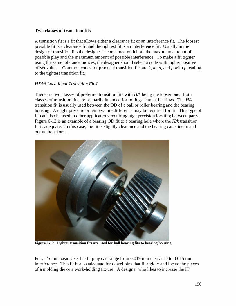
190

Two classes of transition fits

A transition fit is a fit that allows either a clearance fit or an interference fit. The loosest

possible fit is a clearance fit and the tightest fit is an interference fit. Usually in the

design of transition fits the designer is concerned with both the maximum amount of

possible play and the maximum amount of possible interference. To make a fit tighter

using the same tolerance indices, the designer should select a code with higher positive

offset value. Common codes for practical transition fits are k, m, n, and p with p leading

to the tightest transition fit.

H7/k6 Locational Transition Fit-I

There are two classes of preferred transition fits with H/k being the looser one. Both

classes of transition fits are primarily intended for rolling-element bearings. The H/k

transition fit is usually used between the OD of a ball or roller bearing and the bearing

housing. A slight pressure or temperature difference may be required for fit. This type of

fit can also be used in other applications requiring high precision locating between parts.

Figure 6-12 is an example of a bearing OD fit to a bearing hole where the H/k transition

fit is adequate. In this case, the fit is slightly clearance and the bearing can slide in and

out without force.

Figure 6-12. Lighter transition fits are used for ball bearing fits to bearing housing

For a 25 mm basic size, the fit play can range from 0.019 mm clearance to 0.015 mm

interference. This fit is also adequate for dowel pins that fit rigidly and locate the pieces

of a molding die or a work-holding fixture. A designer who likes to increase the IT

191

grades tolerance slightly to H7/k7 would see the maximum possible interference

increasing to 0.023 mm while the maximum clearance remains the same.

H7/n6 Locational Transition Fit-II

H/n is a slightly tighter transition fit than the H/k fit. The fit is frequently used with the

rolling-element bearing fits between the shaft and the bearing bore where a tighter fit is

required to prevent slippage. In Figure 6-12, the fit between the bearings and the shaft is

similar to H7/n6 locational transition fit. A small pressure or temperature difference is

usually required for the locational transition fit. For a 25 mm basic size, the fit play can

range from 0.006 mm clearance to 0.028 mm interference.

Three classes of interference fits

In the design of interference fits the designer likes to assure a minimum amount of

interference to achieve adequate functional rigidity for load transmission capacity. The

shaft offset code usually ranges between p and u with higher order letters leading to

tighter fits.

H7/p6 Locational Interference Fit

This light interference fit is primarily used with high-speed rolling-element bearing fits

between the bearing bore and the shaft when the shaft is subjected to sudden speed

changes. It is also adequate for the fit of plain bearings into their housing. The fit

provides accurate and rigid connection between the mating features such as press-fit

posts. The interference is light and the joint is not expected to carry appreciable forces or

torques. Figure 6-13 shows a gearbox housing with a plain flanged bearing fit to the

housing and a number of gear fit posts. Both the flanged bearing fit and the fit of the

posts into the housing are similar to locational interference fits.

192

Figure 6-13. A light interference fit is adequate for plain bearing fit to its housing

For a 25 mm basic size, the fit interference can range from 0.001 mm to 0.035 mm. The

temperature difference required to achieve a shrink fit for the maximum interference of

0.035 mm is about 130 degrees centigrade for 1-inch diameter fit of steel parts.

H7/s6 Medium Drive Fit

H7/s6 is an interference fit intended to carry moderate loads and torques. In low cost

machines heavy interference fits are often accomplished by creating serrated surface

forms. Figure 6-14 shows an interference gear fit in which the shaft surface is serrated.

With this design a heavy fit can be accomplished with less size precision and lower

forces. The torque carrying performance of this fit, however, is less predictable than a

medium drive fit.

193

Figure 6-14. Extreme precisions and high forces required for a medium drive fit can be avoided by a

serrated shaft surface

For a 25 mm basic size, the fit interference can range from 0.014 mm to 0.048 mm. The

temperature difference required to achieve a shrink fit for the maximum interference of

0.048 mm is about 178 degrees centigrade for 1-inch diameter steel parts. This is usually

the heaviest fit for grey cast iron parts.

H7/u6 Force Fit

Force fits are permanent heavy interference fits intended for steel parts with sufficient

tensile strength and ductility to withstand the required forces and deformations. For a 25

mm basic size, the fit interference can range from 0.027 mm to 0.061 mm. Heavy press

forces or large temperature differences are required to achieve these fits. The temperature

difference required to achieve a shrink fit for the maximum interference of 0.061 mm is

about 226 degrees centigrade for 1-inch diameter steel parts.

Preferred fits provide a good starting point for the selection of best size limits for a

variety of applications. In some cases, analysis, experimentation, or economic reasons

necessitate a deviation from these preferred fits. Adjustments to offsets change the

characteristic of the fit by making it tighter or looser while adjustment of tolerance grades

controls the extent of deviations from the intended tightness or looseness and influence

the cost and quality of the fit.

194

6.7. Dependency of offsets and tolerance grades on basic size

One of the advantages of coded tolerance zones is that they adjust with the basic size.

International tolerance values for the same IT grade increase with feature size. Offset

values also increase with the basic size for any offset designator, except for H and h

designators which always have zero values. This organization of tolerance and offset

values is helpful to the design engineers selecting size limits for proper function. For

example, an f7 size limit designator for a shaft along with an H8 designator for the

mating hole create fits that are generally adequate for journal bearings regardless of the

basic size. As the feature size increases, the joint play also increases to provide adequate

lubrication film thickness for the bearings to operate properly. The combination of

H8/f7, which is the close running fit, provides a functionally similar performance for all

basic sizes.

The size adjusted organization of coded size limits also helps the manufacturing. A shop

personnel seeing an f7 or H8 size limits can quickly assess the required degree of

precision necessary to create them. Manufacturers of components such as bearings can

recommend fit requirements with a single code for all sizes of a class of bearings. For

example, a bearing can be recommended to have an m6 fit for all the sizes in a class. The

use of IT grades was also suggested in Chapter-4 for default profile tolerances to create

adequate tolerance values for both large and small features.

6.8. Tolerance design examples in precision fit applications

With a general understanding of preferred fits a designer can quickly specify the size

limits of features in precision fits. The specified limits would often provide adequate

function using the widest tolerance zones. While coded size limits can be used to

indicate any dimension limits, their use should be limited to features-of-size in direct fit

applications. Coded limits should only be used with preferred or industry-standard basic

sizes for which off-the-shelf tooling or components are available. Finally, despite their

advantages, coded limits present a discrete and limited set of size limits to a design

engineer. When exact size limits needed for the application do not match any coded

limits, the best option is to use the exact numerical size limits. A number of examples

will illustrate the fit design procedures.

Example-1: A ball bearing with a nominal bore diameter of 25 mm is to fit a shaft. The

manufacturer has recommended an m5 tolerance zone for the shaft. Figure 6-15 shows

the fit situation.

195

Figure 6-15. Shaft limits for a ball bearing fit based on manufacturer’s recommendation

The ball bearing bore limits are given as 24.99-25.00 mm. For this situation,

a. Place the required tolerance specification on the shaft drawing.

b. Find the numerical size limits of the shaft using the LAF program.

c. Determine the closest coded limits to the bearing bore size limits.

d. Calculate the fit play range in mm.

Solution

Part a) Since the manufacturer has recommended the limits of the mating feature, the

size limits are directly specified in coded format. Figure 6-16 shows the result.

Ø25m5

Figure 6-16. A ball bearing fit

Part b) Using the LAF Program, the size limits of the shaft corresponding to 25m5 are

25.008 – 25.017 mm.

196

Part c) The bearing bore size tolerance is 0.01 mm. Using the table of IT grades, the

closest size tolerance for a 25 mm feature is 0.009 mm for grade 5. After a few trials

with the LAF program, the 25K5 limits (24.992 – 25.001 mm) is found to be the closest

coded limits to the actual bearing bore limits.

Part d) The loosest fit occurs when the largest bore is matched with the smallest shaft

P1 = 25 – 25.008 = -0.008 mm

The negative sign means this is an interference fit. The tightest fit occurs when the

smallest hole is matched with the largest shaft

P2 = 24.990 – 25.017 = -0.027 mm

Therefore, the fit range is between 0.008 mm interference and 0.027 mm interference.

Example-2: A plain bearing (bushing) is selected to be used with a 10 mm shaft. 10 mm

is the general identifying size also known as the nominal size. The bearing ID is

specified by the manufacturer to have 10H8 limits.

a) Specify the size limits of the 10 mm shaft to obtain a fit similar to a close running

fit.

b) Determine the minimum and maximum play in the fit.

Solution: The size limits for the close running fit for a 10-mm basic size are 10H8 for the

hole and 10f7 for the shaft. Since the hole limits match the close running fit requirement

exactly, the shaft limits must be 10f7. The specifications are shown in Figure 6-17.

10f7 10H8

Figure 6-17. Designation of size limits for the fit between a shaft and a bearing bore

Using the LAF program, the minimum clearance is 0.05 mm and the maximum clearance

is 0.013 mm.

Example-3: The plain bearing used in the previous problem is to fit a hole in a bearing

housing. The size limits on the bearing OD are specified by the manufacturer to be 16h6.

197

a) Specify the size limits of the bearing hole to obtain a fit similar to a locational

interference fit.

b) Determine the closest IT grade to the hole size tolerance.

Solution: Using the LAF program, the minimum and maximum interferences allowed in

locational interference fit for a 16 mm feature are

Pmin = -0.029

Pmax = 0

Also the numerical OD limits for the bearing (16h6) are

Fmax=16.000

Fmin = 15.989

The limits for the bearing hole in the housing can be calculated as

Pmin = Hmin – Fmax -0.029 = Hmin - 16 Hmin = 15.971

And

Pmax = Hmax – Fmin 0 = Hmax – 15.989 Hmax = 15.989

The specifications are shown in Figure 6-18.

15.971

15.989 16h6

Figure 6-18. Designation of size limits for a fit between the bearing OD and the housing recess

The hole size tolerance is 0.018 mm which is exactly an IT7 tolerance grade for a 16 mm

feature size.

Example-4: An off-the-shelf sintered bronze bearing with an ID of 10 (0, +0.02) mm is

to be used to support a 10 mm shaft.

a) Specify the size limits for the mating shaft to obtain a performance similar to a

close running fit.

b) Determine the closest IT grades for both the shaft and the ID of the bearing.

Solution: For a 10-mm basic size, the LAF program indicates a fit play range from

+0.013 mm to +0.050 mm for the close running fit. The minimum play is

198

Pmin = Hmin – Fmax 0.013 = 10 – Fmax Fmax = 9.987 mm

The maximum play is

Pmax = Hmax – Fmin 0.050 = 10.02 – Fmin Fmin = 9.970 mm

The shaft size limits become 10 (-0.013, -0.030).

The tolerance value of 0.017 is slightly more than IT7 = 0.015 mm for a 10 mm size

shaft. The 0.02 mm size tolerance of the bearing hole ID is slightly less than IT8 = 0.022

mm.

Example-5: An off-the-shelf spur gear has bore size limits of 16H7. What shaft size

limits would create a fit similar to a free running fit with this gear? What is the closest IT

grade to the shaft size tolerance? Create a table to show the results when the gear bore

size limits are 16H8, 16H9, 16H10, and 16H11.

Solution: Using the LAF program, the clearance range for a performance similar to free

running fit (16H9/d9) is between 0.05 mm and 0.136 mm. Also for 16H7, Hmin=16.000

mm and Hmax=16.018 mm. The minimum play formula leads to

Pmin = Hmin – Fmax 0.05 = 16 – Fmax Fmax = 15.950 mm

The maximum play formula leads to

Pmax = Hmax – Fmin 0.136 = 16.018 – Fmin Fmin = 15.882 mm

The shaft size tolerance beomes 0.068 mm. This tolerance value is slightly less than

IT10 = 0.070 mm. Therefore the resulting fit has an IT7 on the hole and nearly an IT10

on the shaft. Carrying out the same calculations with other gear hole limits results in the

information indicated in the table below. The first row is the solution above with 16H7

hole limits.

Hole Size

Coded Limits

Hole Numerical

Size Limits

Shaft Numerical

Size Limits

Shaft Size

Coded Limits

16H7 16.000 – 16.018 15.882 – 15.950 ~IT10

16H8 16.000 – 16.027 15.891 – 15.950 IT9-IT10

16H9 16.000 – 16.043 15.907 – 15.950 IT9

16H10 16.000 – 16.070 15.934 – 15.950 ~IT7

16H11 16.000 – 16.110 Not possible Not possible

Note that for the last case, no shaft limits would satisfy the clearance range requirement

because the hole size tolerance is too wide to work even with a shaft with a zero size

tolerance. The hole limits for 16H11 are Hmin=16.000 mm and Hmax=16.11 mm. This

amount of variation already exceed the needed range of play allowed by the free running

fit which is (0.136 - 0.05=0.086 mm). This problem shows the importance of matching

the precision of the two fitting components such that they use comparable tolerances.

Example-6 An 8-mm precision dowel pin with size limits of 8 (+.006, +0.015) mm is to

fit in a mating hole with 8H7 limits. Compare the resulting fits to similar preferred fits.

Solution: The maximum play occurs when both features are at their LMC limit of size

P1 = Hmax – Fmin

199

P1= 8.015 – 8.006 => P1 = +0.009 mm

The maximum interference is

P2 = Hmin – Fmax

P2 = 8 – 8.015 => P2 = -0.015 mm

Comparison of this fit with the preferred fits is shown in the following table.

Fit Loosest fit Tightest fit

This fit +0.009 -0.015

8H7/h6 Locational Clearance Fit +0.024 0

8H7/k6 Locational Transition Fit-I +0.014 -0.010

8H7/n6 Locational Transition Fit-II +0.005 -0.019

8H7/p6 Locational Interference Fit 0 -0.024

Based on the interference values for the loosest fits, this fit with a minimum interference

of 0.009 mm is slightly looser than the H7/k6 which has a minimum interference of 0.014

mm. It is, however, a little tighter than H7/n6 with a minimum interference of 0.005 mm.

Example-7 A 12H7 gear bore is to have an interference load carrying fit with a drive

shaft. It is determined that the minimum adequate radial interference must be 0.004 mm

and the maximum radial interference should be equal to or less than 0.018 mm.

Determine the shaft limits for the interference fit. Compare the results to the preferred

fits.

Solution: The required diametrical interferences are to be between 0.008 mm and 0.036

mm. The minimum interference formula can be used to find the smallest shaft diameter

P1 = Hmax – Fmin = (12+0.018) – Fmin

-0.008 = 12.018 – Fmin => Fmin = 12.026 mm

The maximum interference relation is used to find the maximum shaft diameter

P2 = Hmin – Fmax

-0.036 = 12 – Fmax => Fmax = 12.036 mm

The required size limits of the shaft are 12 (+0.026,+0.036). The total size tolerance on

the shaft diameter is 0.010 mm. This tolerance value is between IT5 grade (0.008 mm)

and IT6 grade (0.011 mm). The following table shows comparison of this fit to preferred

fits.

Fit Loosest fit Tightest fit

This fit -0.008 -0.036

12H7/p6 Locational Interference Fit 0 -0.029

12H7/s6 Medium Drive Fit -0.010 -0.039

12H7/u6 Force Fit -0.015 -0.044

Based on the interference values for the loosest fits, this fit with 0.008 mm minimum

interference is less tight than the H7/s6, the medium drive fit, which has a minimum

interference of 0.010 mm.

200

Example-8 In a hydrodynamic journal bearing application, a designer is expected to

determine the size limits for both the shaft and the bearing hole. The bearing nominal

size is to be 25 mm. Calculations using hydrodynamic lubrication theory show that a

clearance range between 0.025 mm and 0.06 mm would be needed. Determine suitable

size limits for both the shaft and the bearing hole to meet the clearance requirements.

Solution: Following the general guidelines for precision fit design, we decide to have H-

class size limits for the hole. This election leads to the most cost-effective limits for the

fabrication of the bearing hole. Therefore

Hmin = 25.000

Hmax = 25 + tH

The size limits for the shaft are to be determined to meet the fit requirements. We also

select the hole and shaft size tolerances to be the same. Therefore tH = tF = t leading to

Fmax = Fmin + t

Using the minimum clearance formula

Pmin = Hmin – Fmax = (25 – Fmax)

0.025 = 25 – Fmax Fmax = 24.975 mm

Using the maximum clearance formula


0.06 = (25 + t) – (24.975 - t) t = 0.0175 mm

The required size limits of the hole become

Hmin = 25.000

Hmax = 25.017

The required size limits of the shaft become

Fmax = 24.975

Fmin = 24.957

Note that the fourth digit of precision is dropped as an unnecessary level of precision.

The following table shows that the closest preferred fit to the fit in this problem is the

close running fit 25H8/f7. The largest clearance of 25H8/f7, however, exceeds the

needed limit. The next rows in the table show how the fit clearance changes if we

progressively change the tolerance IT values. As indicated in the table, the IT value

change does not affect the tightest fit, only the loosest fit.

Fit Minimum clearance Maximum clearance

This fit (required limits) +0.020 +0.060

25H8/f7 0.020 0.074

25H7/f7 0.020 0.062

25H7/f6 0.020 0.046

In this case, the performance of 25H7/f7 is closest to the required limits. Note that any

possible manufacturing advantage in this specification is in the 25H7 limits and not in the

25f7 limits.

Example-9 A gear is to be fixed to a 15-mm shaft using a Woodruff key. The nominal

width of the Woodruff key is 5 mm and the width is manufactured to limits of 5h9. The

keyway on the shaft is recommended to have an N9 tolerance zone. The keyway width

201

on the hub is recommended to have a JS9 tolerance zone. Figure 6-19 shows the fit

between these members. Determine:

a) Which fit is the tighter fit (key and shaft or key and hub)?

b) The fit limits (clearance or interference) values for key/shaft and key/hub fits.

Figure 6-19. Fit of a key to shaft and hub keyways

Solution

Part-a) The h9/N9 is a tighter transition fit than the h9/JS9 fit. This means the key has a

tighter fit in the shaft keyway than the hub keyway. A better assessment of these fits can

be made by determining the fit limits.

Part-b) Using the LAF program we can determine the following

5N9: (4.97 – 5.00) mm.

5JS9: (4.985 – 5.015) mm.

5h9/N9 fit play or interference: -0.03 to +0.03 mm.

5h9/JS9 fit play or interference: -0.015 to +0.045 mm.

The 5h9/JS9 fit with a maximum play of 0.045 mm in the gear hub is looser than 5h9/N9

fit with a maximum play of 0.030 mm in the shaft.

Example-10: This is the extension shaft tolerancing problem that was presented earlier in

this chapter. Figure 6-20 shows the extension shaft that is driven by a drive shaft that fits

into one end of it and is fixed by a pin.

202

Figure 6-20. Extension shaft assembly

The drive shaft is intended to run at slow speeds and the bearing bore pressure (radial

load) is small. The shaft’s outer diameter fits a bushing. There is a gear fit on the open

end of the shaft that is held in place by a standard Woodruff key. Figure 6-21 shows the

precision fit features of the shaft. Select all the size tolerances of the identified features

necessary to achieve the desired fits.

203

Figure 6-21. The precision fit features of the extension shaft

We will use the following basic size information:

The OD of the extension shaft where the bearing fits is 20 mm

The ID of the shaft where the drive shaft fits is 16 mm

The shaft diameter where the gear fits is 16 mm

The spring pin is 5 mm

The Woodruff key width dimension limits is 5h9

Solution: There are five size limits to be determined:

a) Bearing to shaft fit

b) Drive shaft fit into the extension shaft hole

c) Woodruff key fit

d) Spring pin fit

e) Gear fit

All of these fits are unconstrained fits except the fit of the drive shaft into the extension

shaft hole. The reason for the constrained fit of the drive shaft is that the bearing fit

prevents the extension shaft to freely align itself with the drive shaft. The final solution

reflecting critical size tolerances is shown in Figure 6-22. The selected sizes for each fit

are explained following the figure.

204

Figure 6-22. The critical size tolerances of the extension shaft

The bearing fit: The plain bearing fit to the shaft is chosen to be a close running fit. This

is an adequate fit when speeds are low and the bearing is not intended to carry large

radial loads. In addition, this close fit minimizes the radial runout at the gear end.

Therefore the limits for this fit are selected as 20H8 for the bearing bore and 20f7 for the

shaft.

The drive shaft fit: The drive shaft hole can be initially selected to have 16C9 size limits

to provide enough clearance for the extension shaft to fit the drive shaft and the bearing

simultaneously. Additional location control must be applied to assure the hole would fit

the drive shaft. The details of this fit and location control statement will be explained in

the chapter on location-constrained fits.

Keyway fit: Based on fit recommendations by the manufacturer, the shaft keyway

requires N9 size limits to have a tight fit to the key.

Spring pin fit: A 5-mm nominal size spring pin has been selected. The pin manufacturer

recommends the fitting hole limits to be 5.0 - 5.2 mm in size. These limits are close to

5H13 which correspond to 5.00 - 5.18 mm. The box with CF letters, shown in the figure,

indicates that the two pin holes are to be treated as if they were one continuous feature.

CF stands for continuous feature.

The gear fit: The gear should slide in and out easily. The gear is fixed to the shaft using a

key. The gear bore is assumed to have H size limits. A locational clearance fit

(16H7/h6) has a minimum clearance of zero allowing free assembly. The tolerances are

small enough that the fit is precision and snug. However, the gear fit does not need to be

so precise and so snug. We can relax the IT grades to reduce cost and yet have a

205

functional fit. The precision obtained using average turning process (IT9) would be

adequate for this fit. Therefore, the shaft limits where the gear fits are selected to have

16h9 size limits.

Example-11: Determine the minimum temperature difference in degrees Celsius that is

required to shrink fit two features on steel parts with a 25H7/s6 medium drive fit?

Solution: Thermal expansion can be used to change the size of features to achieve a

shrink fit. The expansion per mm of diameter, or the thermal strain relationship is

TT

The change in feature diameter due to such a temperature change is

TDD

where is the coefficient of thermal expansion. The maximum diametrical interference

in this fit is 0.048 mm. The coefficient of thermal expansion for steel is 10.8*10-6

mm/mm per degrees Celsius. Therefore the temperature change needed is

178)25)(10(8.10048.0 6 TTD degrees C

A temperature differential of about 180 degrees Celsius would be sufficient.

Exercise Problems

1. Use the LAF program and determine the size limits of a 15f6 shaft and a 15H7 hole.

If these features fit together what is the resulting range of clearances or

interferences?

2. What kind of preferred fits are adequate as an initial selection for the following

applications?

i. A disk drive bearing sliding on a ground shaft.

ii. The ID of a ball bearing fitting a rotating shaft subject to heavy shock loading.

iii. The OD of a plain bearing fitting a stationary housing.

iv. The ID of a plain bearing and a shaft in a precision rotation application.

v. A dowel pin fitting tightly into a jig hole – the fit is rigid but removable.

vi. A gear that can be freely assembled on a shaft.

vii. A shaft collar used to fix the axial location of a pulley.

3. What is the size of the fit boundary associated with a hole having size limits of

15H11 and a straightness tolerance of 0.05 mm at MMC? What would be the

theoretical size of a GO gage that would inspect the feature’s straightness tolerance?

4. A disk drive guide rod has a 3g6 specification and is intended to have a sliding fit

with a 3H7 bearing ID. The length of fit is 5 mm. What tolerance specification is

appropriate for the rod such that the sliding fit can be achieved without requiring the

rod to have unneeded precision?

5. The ID of a collar designed for a 12 mm shaft is between 12 mm and 12.013 mm.

Determine the fitting shaft size limits for a performance similar to a free running fit.

206

6. Pick three of the 10 classes of preferred fits and find an actual example for them.

You can find such examples in your gym, machine shop, automobile, labs, your

kitchen or garage, or other ordinary places. Take pictures and explain why the

selected fit matches the preferred fit you picked.

7. Search the internet for “Standard metric drill sizes” for drills up to 25 mm per

ANSI/ASME B94.11M standard. Indicate the millimeter sizes and fractions that are

available starting from the smallest (0.35 mm) size. Also search for tolerances that

regular twist drills can hold in terms of IT grades.

8. Search the internet for typical reamer sizes (Metric sizes per DIN1420 H7) standard.

Do the reamer sizes match the drill sizes? Also look for tolerances that reamers can

hold in terms of IT grades.

9. Search the internet for the applications and standard metric sizes of dowel pins.

What are the main application of dowel pins? The following chart shows a set of

standard metric sizes for dowel pins.

Do these size limits correspond to particular standard coded limits? If yes, specify the

coded limits for each case.

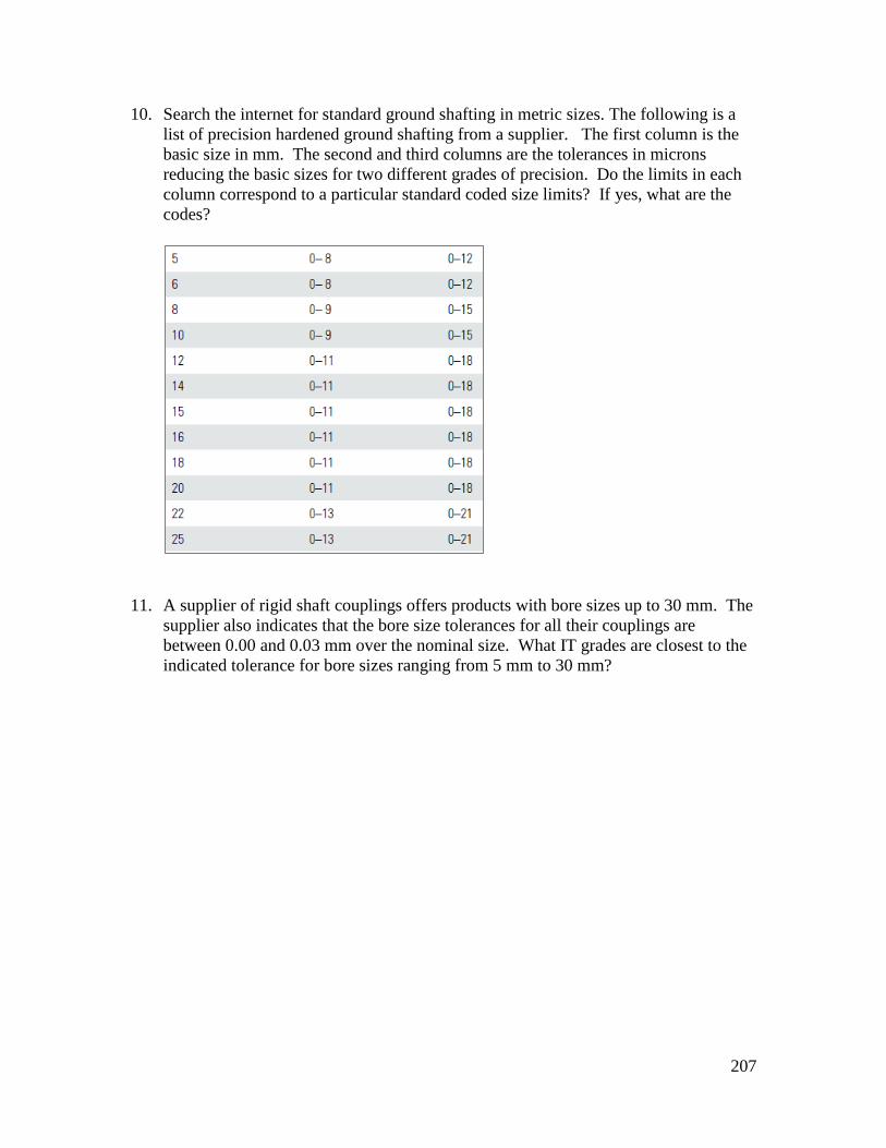
207

10. Search the internet for standard ground shafting in metric sizes. The following is a

list of precision hardened ground shafting from a supplier. The first column is the

basic size in mm. The second and third columns are the tolerances in microns

reducing the basic sizes for two different grades of precision. Do the limits in each

column correspond to a particular standard coded size limits? If yes, what are the

codes?

11. A supplier of rigid shaft couplings offers products with bore sizes up to 30 mm. The

supplier also indicates that the bore size tolerances for all their couplings are

between 0.00 and 0.03 mm over the nominal size. What IT grades are closest to the

indicated tolerance for bore sizes ranging from 5 mm to 30 mm?

208

Chapter 7 Tolerance Design for Orientation-constrained Fits

Between Two Parts

7.1. Overview

Orientation-constrained fits occur when the fitting features are subject to a constraint in

orientation. Fit features are no longer free to center themselves for fit. For example,

consider the simple fit between part1 and part2 in Figure 7-1. In this assembly, the two

plates are intended to firmly contact on the seating surfaces while the stud fits inside the

hole. The design requires that, after assembly, the two seating surfaces be in firm

contact.

part1

part2

Constraint Surface

Figure 7-1. An example of an orientation-constrained fit

The constraint surface creates only one admissible orientation between the two fitting

features. In this case, the constraint surface is the primary orienting surface between the

two parts.

When the design intent is to orient two parts with respect to each other using a firm

contact on two surfaces, the designer must set up the tolerances such that parts that pass

the inspection would fit together while they rest on their contacting surfaces. A typical

and practical example of an orientation constrained fit involves a precision fit between a

stubby boss on one part and a hole in a mating part. The parts are often attached by

threaded fasteners after the precision fit is achieved as shown in Figure-7-2.

209

Figure 7-2. A common application of an orientation-constrained fit

In this example the shallow boss is to fit the hole while the two seating surfaces make full

contact. Figure 7-3 shows an example of a motor shaft and housing fit where two

orientation-constrained fits are used at the two ends of a motor housing to keep the shaft

properly aligned and centered. The shaft is supported by ball bearings.

Cylinder

End Cap

Figure 7-3. A common application of an orientation-constrained fit

210

7.2. The fit boundary and the theoretical gage

The designer’s problem in orientation-constrained fits is similar to the unconstrained fits.

The objective is to tolerance the fitting features such that they always fit together with an

acceptable play. Unlike unconstrained fits in which the amount of play or interference

was critical to the proper function of the fit, constrained fits usually work best when there

is no or little play in the fit.

Consider the simplest case of a pin and a hole such as the one shown in Figure 7-4. The

design intent is to precisely orient the two parts relative to one another using the seating

surfaces. The fit features then center the two parts. Usually this kind of fit allows little

fit play and is designed for precision orienting and locating of one part with respect to a

mating part. In this figure, the fit play is exaggerated for illustration.

Figure 7-4. A simple orientation-constrained fit

To assure a clearance fit, imagine a fit boundary such as the one shown as dashed lines in

Figure 7-5.

211

Fit

Boundary

Perfect Flat Surface

Figure 7-5. Fit is assured when the pin fits inside the fit boundary while the seating surface aligns

with the flat surface. Also, the hole fits outside the fit boundary when its seating surface aligns with

the flat surface

The pin must fit inside the fit boundary and the hole must fit outside of the same fit

boundary while the seating surfaces are in full contact. To assure fit, a plane representing

the seating surface should be added to the fit boundary to define the theoretical gage.

The logic of fit is simple and only involves checking each part separately against their

theoretical gages. Figure 7-6 shows two acceptable parts passing the theoretical

inspection successfully.

24

Figure 7-6. The theoretical gage drawn in dashed lines accepts both parts for fit

A physical hard gage can often be made to test the actual features for fit-related tolerance

specifications as shown in Figure 7-7.

212

24

2424

Physical gage for

checking the Hole

Physical gage for

checking the Pin

Figure 7-7. Physical gages for checking the Pin and the Hole for fit

The GDT statements that define the theoretical gage for orientation-constrained fits must

describe the fit boundary sizes and identify the constraint surfaces to be used as datum

simulators. The following text version of the tolerance statement captures the theoretical

gage information for the pin:

Make the pin such that it would fit inside a 24-mm cylinder while the shoulder is

resting on the datum plane

This statement results in a 24-mm fit boundary and a datum plane perpendicular to it just

like the dashed line geometry shown in Figure 7-6. For manufacturing purposes the

above tolerance instruction is difficult to use. An alternative specification in terms of

feature local sizes and a limit on deviation from perpendicularity is more helpful in

manufacturing as these geometric precisions directly relate to process capabilities and can

be measured during manufacturing with common inspection tools. We can use the

following alternative description of the fit boundary:

Make the pin such that its maximum cross-section size would not exceed 24 mm. If

the cross-section size is 24-mm, the feature must be perfectly perpendicular to the

datum surface. When the cross-sectional size is smaller than 24-mm, the shaft axis

can tilt by the difference between the actual size and the MMC size of 24 mm.

Note that the deviation from perpendicularity is measured as a distance, not an angle, as

shown in Figure 7-8. In this case the deviation from perfect perpendicularity is 0.3 mm.

213

0.3

Figure 7-8. Deviation from perpendicularity is measured as a distance not an angle

As an example, the axis of a 23 mm pin can be slanted by as much as 1 mm and still fit

inside the 24 mm boundary. The axis of a 20 mm pin can be slanted by as much as 4 mm

and pass the tolerance statement as well. Obviously the above tolerance statement is only

concerned with assuring fit without caring about maximum possible play in the fit.

Another statement would be required to limit the maximum play by excluding pins that

are too small. Adding a minimum size limit of 23 mm and abbreviating the text, the new

tolerance statement requires the following two parts:

Make the pin such that its cross-section size would be between 23 and 24 mm.

If the cross-section size is 24-mm (at MMC), then the feature axis must be

perfectly perpendicular to the datum plane.

In the second statement, it is understood by the manufacturing and inspection that what is

required is a fit boundary of size 24 mm and the minimum local size is to be 23 mm. The

extreme orientation of the pin that would be acceptable based on the tolerance description

above is shown in Figure 7-9. Note that while the fit is always possible in manual

assembly, it is not necessarily achievable if the fit is to be made by a pick and place

robot. This is because humans can find the most favorable alignment for fit such that the

pin would snap in place. A robot may not be able to find the best alignment for fit.

1

23

Figure 7-9. Maximum perpendicularity deviation for a 23-mm feature when fit boundary is 24-mm

214

The design engineer must now translate the tolerance requirements presented as text into

standard geometric tolerancing symbols and place those symbols on the drawing. Figure

7-10 shows the way it must be indicated on the drawing:

Ø 23-24

Ø 0 AM

A


The manufacturing engineers read this statement as: “the feature cross-sectional size is to

be between 23 and 24 mm. This feature is to be perpendicular to datum A to within 0

mm at MMC.”

The designer can make the fit boundary larger than the MMC size of the pin by using a

non-zero perpendicularity for tolerance value. For example, to define a 25 mm fit

boundary for a pin with 23-24 mm cross-sectional size limits, we must specify a 1 mm

perpendicularity tolerance at MMC as shown in Figure 7-11.

215

Ø 23-24Ø 1 AM

A


In this case, a 24-mm pin is allowed to tilt 1 mm while a 23-mm pin can tilt 2 mm. For a

pin, the size of the fit boundary is the sum of the geometric tolerance value and the MMC

size of the pin. For a hole, the size of the fit boundary is the MMC size of the hole minus

the geometric tolerance value.

The fit formulas developed for the unconstrained fits remain unchanged. The only

difference is that the geometric tolerance changes from the straightness or flatness

tolerance to perpendicularity tolerance. The minimum play formula is

Pmin = (Hmin – Fmax) – (TH + TF)

To assure a zero-clearance fit in an orientation-constrained fit the sum of geometric

tolerances applied to both features must be equal or smaller than the difference between

the fit features MMC sizes


In this formula TH and TF are the perpendicularity tolerance values at MMC indicated in

the tolerance statement. Also, Hmin and Fmax are the MMC sizes of the hole feature and

the pin feature respectively.

In order to have at least a minimum play of Pmin in the clearance fit, we can increase the

difference between the fit boundaries of the mating features by adding a Pmin to the hole

fit boundary, or by subtracting a Pmin from the pin fit boundary. The resulting tolerance

relationship to assure a minimum play of Pmin becomes

TH + TF ≤ Hmin – Fmax - PminIn the case of unconstrained precision fits the requirement for a minimum play was

critical to the function of the joint in many applications. In the case of orientation-

constrained fits or location-constrained fits, the need to have an assured minimum

clearance is rare. In most applications involving constrained fits, the objective is for the

features to simply fit together with as little play as possible.

216

The maximum play in a fit occurs when the two fitting features are made at their least

material condition and are at perfect orientation relative to their datum surfaces. The

maximum play formula based on LMC sizes is


Where Hmax and Fmin are the LMC hole and pin feature sizes respectively. Figure 7-12

shows the condition leading to maximum play for a 24-25 mm hole fitting a 23-24 pin.

2325

Figure 7-12. Perfect-perpendicularity at LMC leads to maximum play in a fit

We can also write the maximum play formula in terms of tolerances of size and

orientation as

Pmax = tH + tF + TH + TF + Pmin

Where tH and tF are the size tolerances of the hole and pin respectively. Note that in order

to minimize the play we should use the smallest tolerances of size and orientation and

also set up the fit with a zero minimum play.

7.3. A word on inspection

Hard gaging is the direct method of checking all fit-related tolerance statements but if

physical gaging is not feasible, the features can be inspected using other measurement

tools. The inspection procedure attempts to determine whether the combination of cross-

section size and out-of-perpendicularity would allow a feature to remain within its fit

boundary. Figure 7-13 shows the situation for a 24-mm fit boundary where the size

limits are 23-24 mm and the perpendicularity tolerance is zero at MMC.

217

23.4

0.8

24 Fit Boundary

Datum

AME

dial moves normal

to datum

Figure 7-13. A dial indicator readout and the local size determine whether a feature violates the fit

boundary

The verification is a simple geometry problem. Here, the combined effect of feature size

and its axis out-of-perpendicularity exceeds the fit boundary by 0.2 mm. The

combination of measured size and measured axis tilt defines a boundary similar to the fit

boundary but with a size that just fits the feature. This measured boundary is an

equivalent perfect-form representation of the actual feature for fit purposes. The formal

name of this perfect-form boundary is orientation-constrained actual mating envelope or

orientation-constrained AME of the feature. In the example shown in Figure 7-13, the

size of the orientation-constrained AME for the shaft feature is 24.2 mm. The size of the

unconstrained AME is slightly less than 23.4 mm.

7.4. MMC boundary as fit boundary

In the chapter on unconstrained fits it was argued that, when possible, the use of the

MMC boundary as the fit boundary would be the best choice. That argument is also valid

for the case of orientation-constrained fits and tolerance of perpendicularity. For

example, consider the two options for defining a fit boundary of size 24 mm as shown in

Figure 7-14.

218

Ø 1 AMA A

Ø 0 AM

Ø 22-24Ø22-23

Figure 7-14. An example of an orientation-constrained fit

The two features perform similarly in their ability to fit a mating feature because both

have the same size fit boundary. The two features also have the same LMC sizes so they

perform similarly in their potential maximum play performance. The specification on the

right side of the figure that allows 1-mm perpendicularity at MMC is inferior to the

specification with zero perpendicularity tolerance. This is because the statement with 1-

mm perpendicularity tolerance does not accept a feature that is 23.5 mm even when the

feature is perfectly perpendicular to datum-A and easily fits inside the 24 mm fit

boundary. This means that in a fit situation, a non-zero geometric tolerance can exclude

functionally acceptable parts. The use of zero geometric tolerance provides the widest

manufacturing tolerances for the same fit performance. For fit purposes, zero orientation

option makes the variations in size and orientation interchangeable both ways. A size

close to LMC leaves maximum tolerance for orientation and a nearly perfect orientation

leaves maximum tolerance for size.

To define the MMC boundary as the fit boundary requires the geometric tolerance value

at MMC to be zero. This form of specification combines the tolerance of size and the

tolerances of orientation into a wider tolerance of size. The fit formula when zero

orientation tolerance is used for both fitting features becomes

H0min – F0max ≥ 0

Setting up orientation-constrained fits with a zero geometric tolerance option is also

simple and leads to economic advantages. For example, consider an orientation-

constrained fit for a pair of features with the following requirements:

Nominal size: 15 mm

Minimum play 0 mm

Maximum play 0.1 mm

The size limits for the features can be easily found by dividing the maximum play

between the hole and the pin features. For example, dividing the 0.1 mm equally

between the two features leads to size tolerance of 0.05 mm for both features. The pin

219

feature size limits would then become (14.95 – 15.00) and the hole limits would become

(15.00 – 15.05). Both features border the basic size of 15 mm with holes slightly larger

than the basic size (similar to H-class offset) and pins slightly smaller than the basic size

(similar to h-class offsets). We have already seen in Chapter-6 that these types of size

limits are economically preferred, especially when nominal sizes are selected from the

list of preferred sizes or available standard sizes.

A zero orientation tolerance at MMC is often implied with standard parts. For example, a

standard bolt with a maximum size of 10 mm is implied to have zero perpendicularity

tolerance at the maximum size of 10 mm with respect to the seating shoulder of the bolt.

This means the bolt with fit a 10 mm hole while the bolt head is firmly seated.

7.5. Situations where MMC modified tolerances cannot be used

When the size of a feature needs to be controlled with precision for any reason, the size

tolerance must be specified as needed. In such cases the size tolerance should not be

expanded to include the orientation tolerance. A common example is when a hole feature

accepts a press-fit insert as shown in Figure 7-15.

Insert

Figure 7-15. The hole feature in the plate must have size limits for interference fit to the insert

In this situation, the hole in the plate must have a precise size tolerance in order to have

the required light interference fit. When the hole is toleranced for fit, its size and

orientation tolerances must be specified separately without MMC qualification. This is


220

8H7Ø 0.5 A

A

Figure 7-16. Tolerancing of the hole feature for fit cannot use the zero perpendicularity format

Note that this assembly involves three parts and we can no longer check the fit using fit

boundary method. The methods for checking the fit of multipart assemblies will be

presented in Chapter-11.

7.6. Datum feature flatness

The objective of an orientation-constrained fit is to accurately fix the relative orientation

of two parts and the datum features serve this purpose. If either of the datum features is

not flat enough to prevent rocking, the final orientation relationship between the two parts

becomes unpredictable and subject to the manner of final assembly. For example, in

Figure 7-17 the seating datum surface of the part on the left is not flat enough and as a

result the contact is subject to rocking. The final relative orientation between the two

parts becomes dependent on which screw is tightened first. While the fit can be

accomplished, the important relationship, which is the relative orientation between the

two parts, becomes unpredictable. This can create misalignments that would compromise

the function of the assembly or the fit of other parts in multipart fits.

221

Figure 7-17. Uneven contact surfaces can create unpredictable results

Applying sufficient flatness control is the method of preventing or reducing the

possibility of rocking. In all orientation-constrained fits, the flatness of the datum surface

must be controlled to the extent required to prevent rocking. An example of specification

is shown in Figure 7-18.

AØ 0 AM

0.25

23 - 24

Figure 7-18. Adequate flatness control is necessary on all contact surfaces

In some cases a small amount of rocking may not lead to adverse consequences.

However, when the datum surfaces are used in precision applications, any rocking would

be unacceptable. Such datum surfaces on typical machine parts must be finish milled or

made with a process that can create a surface comparable to a finish milled surface.

222

When large areas are to be used as orienting datums, it is best to create raised pads that

would reduce the possibility of rocking while at the same time reduce the cost of

machining. Figure 7-19 shows an example for the helical gearbox presented before.

Raised Milled

Surface

Figure 7-19. Raised and machined surfaces are common in the design of cast parts

Note that the four mounting surfaces of the gearbox housing have raised surfaces which

are milled to create a non-rocking support. The top surface of the housing, on the other

hand, does not employ raised surfaces because it is used for sealing purposes.

Example-1: Figure 7-20 shows the turning support assembly along with a representation

of a lathe machine and a part. The turning support assembly is an attachment to a lathe

machine that provides additional support to a long part in the turning process. The

function of turning support is similar to the lathe tail stock but the turning support can be

positioned to support the part in the middle rather than the end of the part. Custom insert

sizes can be made to adapt the turning support to various part sizes.

223

Figure 7-20. Turning support assembly

The fit to be specified is between the base plate rail and the turning support slot. We need

to dimension and tolerance the slot and rail features in turning support and base plate for

a fit with as little play as possible. The basic size of the slot is 76 mm and we know that

a finish milling process would create adequate precision for these parts. After specifying

the tolerances we like to calculate the maximum play in the slot/rail fit.

Solution: The milling process can hold a total combined size and perpendicularity

tolerance of 0.12 mm for this 76 mm feature. Using zero geometric tolerances and equal

tolerances for the slot and rail, the size limits of the slot becomes 76 (-0, +0.12) mm and

the size limits of the rail becomes 76 (-0.12, +0) mm. The maximum play when zero

geometric tolerances are used becomes the sum of size tolerances

Pmax = (76 + 0.12) – (76 - 0.12) = 0.24

To complete the tolerance requirements for this fit, we need to apply a flatness control to

the sliding datum surface. The surface must be sufficiently flat to assure firm seating and

to prevent rocking. For a milling process, a flatness of 0.025 mm can be expected for the

sliding surface of the slot feature and a flatness of 0.05 mm can be expected for the rail

feature. Figure 7-21 shows the final tolerance statements for the turning support

necessary for the fit to the base plate.

224

Figure 7-21. Tolerance of slot feature for an orientation-constrained fit

Figure 7-22 shows the final tolerance statements for the base plate necessary for the fit of

the slot and rail. Since the length of fit is smaller than the length of the base plate, the

perpendicularity tolerance can be specified to be per fit length.

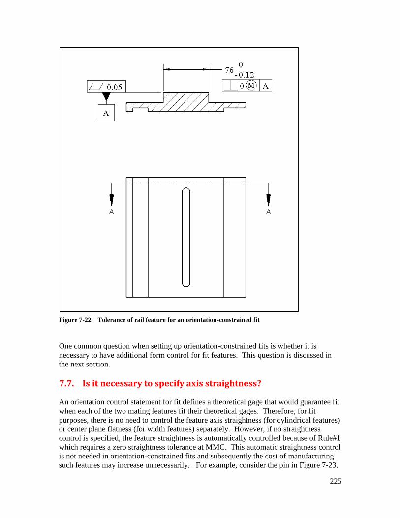
225

Figure 7-22. Tolerance of rail feature for an orientation-constrained fit

One common question when setting up orientation-constrained fits is whether it is

necessary to have additional form control for fit features. This question is discussed in

the next section.

7.7. Is it necessary to specify axis straightness?

An orientation control statement for fit defines a theoretical gage that would guarantee fit

when each of the two mating features fit their theoretical gages. Therefore, for fit

purposes, there is no need to control the feature axis straightness (for cylindrical features)

or center plane flatness (for width features) separately. However, if no straightness

control is specified, the feature straightness is automatically controlled because of Rule#1

which requires a zero straightness tolerance at MMC. This automatic straightness control

is not needed in orientation-constrained fits and subsequently the cost of manufacturing

such features may increase unnecessarily. For example, consider the pin in Figure 7-23.

226

Ø 23-24Ø 1 AM

A

Figure 7-23. A feature set up for an orientation-constrained fit

In this example, if the pin feature is made at 24 mm (its MMC size), it can tilt as much as

1 mm and still fit inside the fit boundary of 25 mm. The pin may instead bend as much

as 1 mm and still fit inside the gage. However, Rule#1 prevents any bending when the

feature is 24 mm in size or at MMC. The result is the rejection of a perfectly functional

feature due to the default straightness tolerance requirement of Rule#1. The automatic

application of Rule#1 in this case is unnecessary.

To prevent the automatic application of zero straightness at MMC, the design engineer

can use the independency symbol following the size tolerance as shown in Figure 7-24.

With the independency symbol, the 24mm features can tilt or bend 1 mm as the

requirement of perfect straightness at MMC no longer applies.

Ø 23-24Ø 1 AM

A

I

Figure 7-24. With the independency symbol the feature need not have perfect straightness at MMC

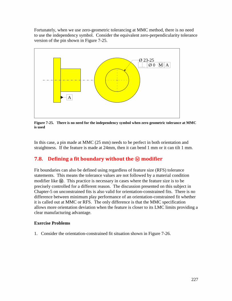
227

Fortunately, when we use zero-geometric tolerancing at MMC method, there is no need

to use the independency symbol. Consider the equivalent zero-perpendicularity tolerance

version of the pin shown in Figure 7-25.

Ø 23-25Ø 0 AM

A

Figure 7-25. There is no need for the independency symbol when zero geometric tolerance at MMC

is used

In this case, a pin made at MMC (25 mm) needs to be perfect in both orientation and

straightness. If the feature is made at 24mm, then it can bend 1 mm or it can tilt 1 mm.


Fit boundaries can also be defined using regardless of feature size (RFS) tolerance

statements. This means the tolerance values are not followed by a material condition

modifier like m. This practice is necessary in cases where the feature size is to be

precisely controlled for a different reason. The discussion presented on this subject in

Chapter-5 on unconstrained fits is also valid for orientation-constrained fits. There is no

difference between minimum play performance of an orientation-constrained fit whether

it is called out at MMC or RFS. The only difference is that the MMC specification

allows more orientation deviation when the feature is closer to its LMC limits providing a

clear manufacturing advantage.

Exercise Problems

1. Consider the orientation-constrained fit situation shown in Figure 7-26.

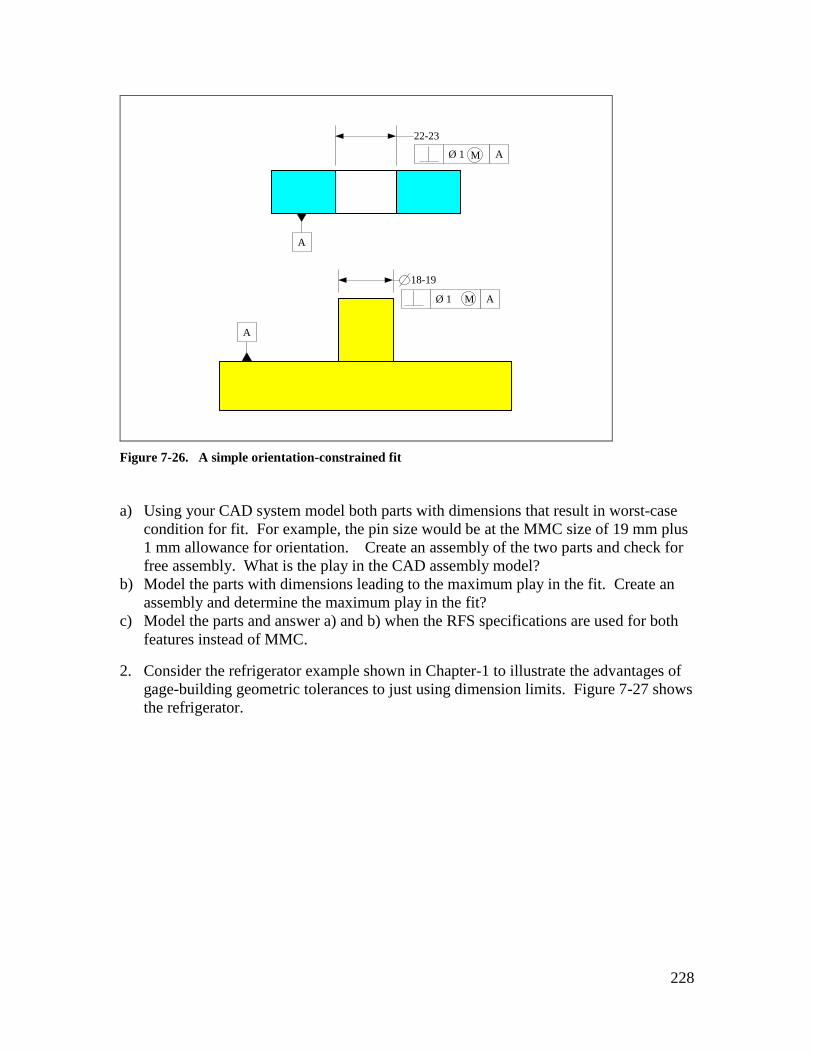
228

Ø 1 A

Ø 1 A

A

A

18-19

22-23

M

M

Figure 7-26. A simple orientation-constrained fit

a) Using your CAD system model both parts with dimensions that result in worst-case

condition for fit. For example, the pin size would be at the MMC size of 19 mm plus

1 mm allowance for orientation. Create an assembly of the two parts and check for

free assembly. What is the play in the CAD assembly model?

b) Model the parts with dimensions leading to the maximum play in the fit. Create an

assembly and determine the maximum play in the fit?

c) Model the parts and answer a) and b) when the RFS specifications are used for both

features instead of MMC.

2. Consider the refrigerator example shown in Chapter-1 to illustrate the advantages of

gage-building geometric tolerances to just using dimension limits. Figure 7-27 shows

the refrigerator.

229

Figure 7-27. The refrigerator and the doorway

Suppose the doorway width is exactly 835 mm and its form and orientation with respect

to the floor are perfect.

a) Write a set of instructions using length and angle measurements to decide whether

the refrigerator would pass through the door opening. Show the results for an

example by making up some measurement data.

3. Find an actual example of an orientation-constrained fit. You can find such examples

in your gym, machine shop, automobile, labs, your kitchen or garage, or other

ordinary places. Take pictures and explain why the fit represents an orientation-

constrained fit.

230

Chapter 8 Tolerance Design for Location-constrained Fits

Between Two Parts

8.1. Overview

Location-constrained fits are the most common type of fit between two parts. In

location-constrained fits a feature’s location as well as orientation is constrained with

respect to a datum frame. Figure 8-1 shows an example of a simple location-constrained

fit involving a single fit feature, a primary orienting datum surface, and a secondary

orienting and locating datum surface.

Figure 8-1. An example of a location-constrained fit

The relative orientation of the two parts is constrained by a planar seating surface. This

seating surface is the primary orienting/locating datum surface (or primary datum). The

other contacting surface is the secondary orienting/locating surface (or secondary

datum). The secondary datum creates additional constraint between the two parts. With

these two datum features in contact, the two parts can still slide with respect to each other

and are not completely fixed together. In many applications, a third datum surface is

used to completely fix the two parts with respect to each other. Figure 8-2 shows the 2D

view of the assembly.

231

Primary Orienting

Surface

Secondary Orienting and

Locating Surface

Figure 8-2. An example of a location-constrained fit in 2D view

The fitting features can be cylindrical or width features. Fasteners are usually employed

to enforce the full contact of the primary datum features.

8.2. The fit boundary and the theoretical gage

To assure fit, the design engineer must set up a fit boundary for the fit features and then

identify the primary, secondary, and possibly tertiary datum surfaces to define a

theoretical gage. The gage geometry must then be communicated to the manufacturing to

define the necessary precision requirements. Figure 8-3 shows such a theoretical gage for

the fit situation in Figure 8-2. In this example, the designer has chosen a 24 mm fit

boundary. The theoretical or basic location of the feature relative to the locating datum is

60 mm.

Primary Datum

Simulator

Secondary Datum

Simulator

60

24

Fit Boundary

Figure 8-3. For location constrained fits the fit boundary is located relative to the datum planes

232

In order for the two fit features to fit together both parts must make full contact with the

primary datum and also make a firm contact with the secondary datum. After the datum

contacts are established, the hole feature must fit outside the fit boundary and the pin

feature must fit inside the fit boundary. An example of such a fit is shown in Figure 8-4

60

24

Fit Boundary

Figure 8-4. Fit is assured when the mating features clear the gage

Although the pin feature clearly deviates from the theoretical location of 60 mm, it still

fits inside the fit boundary because it is made close to its more slender LMC size. Just

like orientation-constrained fits, the datum features must be flat enough to prevent the

parts from rocking on the datum surfaces. In addition, the secondary datum must be

specified to be sufficiently perpendicular to the primary datum surface to prevent fit

problems. Designers must specify the datum features to be sufficiently flat and

perpendicular to each other before using them in precision fit applications.

The GDT statement that conveys the theoretical gage geometry and method of gaging

must disclose the following four sets of information:

1. A statement to describe the fit boundary size.

2. The identification of datum surfaces to be added to the fit boundary as datum

simulators.

3. The theoretical location of the fit boundary with respect to the datum frame.

4. The order in which the datum features are to be aligned against the gage datum

simulators during inspection (datum priority).

The first three items in the above list describe the geometry of the theoretical gage while

the fourth item prescribes the order in which the part is to be constrained by the simulated

datums of the gage. In addition to assuring fit the designer must control the fit play by

controlling the LMC sizes of the fit features. In the case of the previous example in

233

Figure 8-2, the design engineer communicates the theoretical gage geometry using GDT

statements shown in Figure 8-5 for the part with the pin feature.

23-24

A

B

Ø 0 A BM

60

Figure 8-5. Description of 24 mm fit boundary using GDT position tolerance

In this position tolerance statement, the MMC size of the feature along with the tolerance

value of zero at MMC define the size of the fit boundary to be 24 mm. The datums are

identified and labeled as A and B and the tolerance statement specifies A as the primary

datum and B as the secondary datum. Note that letter designations A and B do not imply

anything regarding whether they are primary datum or secondary datum – it is the order

in which they appear in the tolerance statement that makes that assignment. The

theoretical location of the fit boundary with respect to the locating datum is given by a

dimension of 60 mm.

The manufacturing interprets the fit boundary requirement as they appear explicitly in the

tolerance statement as follows:

Make the pin such that its cross-sectional size will be between 23 and 24 mm.

If the cross-section size is 24 mm (or at MMC), then the pin must be perfect in its

form, orientation, and location. When the pin is made at its LMC size of 23 mm,

then its combined form, orientation, and location deviation can be as much as 1

mm.

One extreme shape of the pin that would be acceptable based on the tolerance description

above is shown in Figure 8-6.

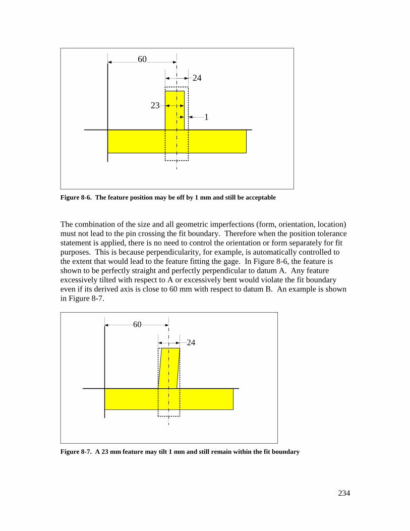
234

60

24

23

1

Figure 8-6. The feature position may be off by 1 mm and still be acceptable

The combination of the size and all geometric imperfections (form, orientation, location)

must not lead to the pin crossing the fit boundary. Therefore when the position tolerance

statement is applied, there is no need to control the orientation or form separately for fit

purposes. This is because perpendicularity, for example, is automatically controlled to

the extent that would lead to the feature fitting the gage. In Figure 8-6, the feature is

shown to be perfectly straight and perfectly perpendicular to datum A. Any feature

excessively tilted with respect to A or excessively bent would violate the fit boundary

even if its derived axis is close to 60 mm with respect to datum B. An example is shown

in Figure 8-7.

60

24

Figure 8-7. A 23 mm feature may tilt 1 mm and still remain within the fit boundary

235

The size of the fit boundary for external or pin features is the sum of the MMC size of the

feature and the geometric tolerance at MMC, in this case, the position tolerance

FBF = Fmax + TF

And for a hole feature

FBH = Hmin – TH

In this formulas TH and TF are the position tolerance values at MMC as indicated in the

tolerance statement. Also, Hmin and Fmax are the MMC sizes of the hole feature and the

pin feature.

In the direction where the two parts can have free play, the fit formulas developed for the

orientation-constrained fits remain unchanged. The minimum play formula is

Pmin = (Hmin – Fmax) – (TH –TF)

In the direction where the features are fixed and there is no free play, there can be a

minimum gap between the mating features. The minimum gap occurs between the two

adjacent surfaces of the fit features as seen in Figure 8-8. In this figure, the fit boundaries

are shown in dashed lines and are not equal in size.

60

Gap

Figure 8-8. When fit boundary of pin is smaller than the fit boundary of the hole, there will be a

guaranteed minimum gap in the fit.

The minimum gap formula is

Gmin = ½(Hmin – TH – Fmax – TF)

For an acceptable zero-clearance fit (Gmin = 0) the fit formula remains as before


When zero position tolerance is used, the fit formula becomes

H0min – F0max ≤ 0

Unlike unconstrained fits, there is rarely a need to have an assured minimum gap in a

location-constrained fit. For all such fits, Gmin=0 is often most desirable.

236

In the direction where the parts can slide, the maximum play formula based on LMC

sizes is determined as


In the direction where the two parts are fixed with respect to each other, the maximum

gap occurs when both features are made at their LMC limit of size. When Gmin is set to

zero, the formula for maximum gap is

Gmax = Hmax – Fmin

For a numerical example, suppose the hole feature has size limits of 24-25 mm and a

position tolerance of zero at MMC and the pin feature size is 23-24 mm with a position

tolerance of zero at MMC. The minimum gap is zero when both features are 24 mm in

size, and the maximum gap can be 2 mm when both features are at LMC as shown in

Figure 8-9. The shaft at LMC size of 23 mm has shifted to the left relative to its

theoretical location by 0.5 mm while the hole at LMC size of 25 mm has shifted to the

right by 0.5 mm.

60

25

23

Figure 8-9. When the fit boundaries of pin and hole have the same size and the minimum gap is zero,

the maximum gap is determined by the LMC sizes of the hole and the pin.

In the chapters on unconstrained fits and orientation-constrained fits it was argued that

the use of the MMC boundary as the fit boundary was the best choice. That argument is

also valid for the case of location-constrained fits and position tolerances when there is

no objection to the feature being made at a wider range of sizes. Zero position tolerance

at MMC combines the size and location tolerances into a larger size tolerance. The zero-

position tolerance at MMC not only provides maximum flexibility in manufacturing but it

also makes the tolerancing calculations easier.

8.3. Datum priority

A position tolerance statement prescribes a theoretical gage by defining a fit boundary

that is oriented and located with respect to datums. While the theoretical gage has datum

plane simulators that are perfectly flat and perfectly perpendicular to each other, the

237

actual part that is to be checked against this gage would not have perfect datum surfaces.

When there are multiple contact datum features, the order of constraining the part to the

gage is important. The designer must carefully set up the order of datum contacts to

mimic the way the part is to fit into the assembly. Consider the assembly shown in

Figure 8-10.


In this fit, the design intent is to orient the two parts with respect to each other using the

larger horizontal seating surfaces. There are fasteners that enforce this complete and firm

contact in assembly. The designer must set up the problem such that the seating surfaces

are selected as the primary orienting surfaces.

By specifying the datum priority, the design engineer can ensure that the part is made and

gaged in a way that mimics its proper place in the actual assembly. If gaging and the

actual application do not match, the parts may not fit properly. In this case by explicitly

identifying the seating surfaces as the primary orienting datums, the designer instructs the

inspection personnel how to gage the part and when to accept it. This can be done by

calling the seating surface (labeled A) to be the primary orienting surface as indicated in

Figure 8-11.

238

Ø 0 A BM

23 - 24

A

B

Figure 8-11. Datum-A is designated as the primary datum and datum-B as the secondary datum

When the part with the pin feature is manufactured, the datum surfaces do not come out

perfectly perpendicular. Therefore a pin that is made to be precisely perpendicular to the

seating surface (surface A) would not be precisely parallel to the locating edge surface

(surface B).

In the part shown in Figure 8-12 the pin is correctly made to be primarily perpendicular

to the seating surface (surface A). The incorrect alternative, in this case, is to make the

pin parallel to the side surface (Surface B).

Figure 8-12. The pin feature is well-made as its orientation (perpendicularity) is precise with respect

to the primary datum feature

239

This part passes the gage properly as shown in Figure 8-13. Note that the gaging

correctly makes full contact with the seating or primary datum-A. If the gage incorrectly

makes full contact with the B surface instead of A surface, the pin will not clear the gage.

Figure 8-13. The part clears the gage and is acceptable.

This part is acceptable and fits its mating part as intended when used in assembly as


Figure 8-14. The part fits the assembly just as it fits the gage it passed.

Fit problems occur when the design engineer overlooks the importance of the primary

orienting datum and specifies surface B to be the primary datum that orients the two parts

with respect to each other. It happens quite often because engineers intuitively do not see

the importance of the orienting surface and only consider the pin’s distance to the side

240

surface as the only relevant geometric criterion. This incorrect specification scheme is

shown Figure 8-15.

Ø 0 BM

23 - 24

A

B

Figure 8-15. Incorrect specification of the primary orienting datum given the manner of assembly

This specification tells the manufacturing that the orientation relationship between the pin

and surface A is less important than B. When the manufacturing sees that only the edge

datum (surface B) is called out in the position statement they try to make the pin feature

more parallel to the edge datum surface and at a distance of 60 mm from that edge datum.

Figure 8-16 shows an exaggerated shape for the purpose of illustration.

A

B

Figure 8-16. The pin feature is well-made as its orientation (parallelness) is precise with respect to

the primary datum feature (B in this case)

241

The inspector also attempts to gage this according to the specification which calls for full

contact of gage with surface B. In this manner the gage fits the part as shown in Figure

8-17 and subsequently the part is accepted. The gage simply verifies that the pin is

precisely parallel and at a precise distance from surface B exactly as the design engineer

specified it.

Gage

Part

Figure 8-17. When checking the part, the side surface (datum-B) is aligned with the datum feature

for full contact

This figure also shows what is going to happen during the actual assembly because the

gage simply acts as a mating part. This manner of assembly is clearly not what the

designer intended. It only occurred because the designer overlooked the fact that datum-

A should be the primary orienting surface during assembly, not datum-B. Adding datum-

A as the secondary datum does not change anything. In fact, adding datum-A as a

secondary datum can be confusing to manufacturing because it neither orients nor locates

the subject feature.

8.4. Datum frame precision

As in the case of orientation-constrained fits, the primary orienting datum feature should

be flat enough not to rock. The secondary datum feature must also be sufficiently flat to

prevent rocking. The secondary datum, however, has restricted freedom and its flatness

need not be controlled with as much precision as the primary datum. In addition, the

secondary datum feature’s perpendicularity with respect to the primary datum must be

controlled with high accuracy. The tertiary datum’s orientation with respect to the

primary and the secondary datum features must also be controlled with sufficient

accuracy. When the perpendicularity tolerance is specified to be small enough to prevent

rocking, there is usually no need for additional flatness tolerance.

Consider a typical case where a secondary datum locates two mating parts with respect to

each other. There would be adverse locating consequences when the secondary datum is

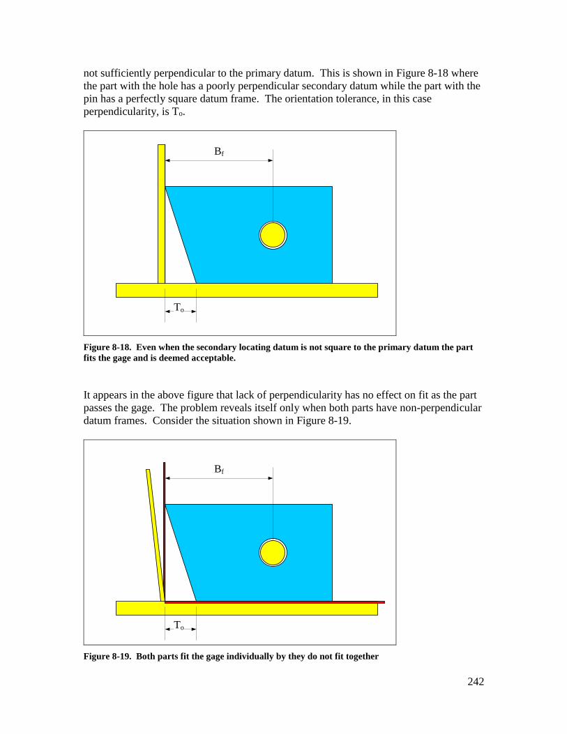
242

not sufficiently perpendicular to the primary datum. This is shown in Figure 8-18 where

the part with the hole has a poorly perpendicular secondary datum while the part with the

pin has a perfectly square datum frame. The orientation tolerance, in this case

perpendicularity, is To.

Bf

To

Figure 8-18. Even when the secondary locating datum is not square to the primary datum the part

fits the gage and is deemed acceptable.

It appears in the above figure that lack of perpendicularity has no effect on fit as the part

passes the gage. The problem reveals itself only when both parts have non-perpendicular

datum frames. Consider the situation shown in Figure 8-19.

Bf

To

Figure 8-19. Both parts fit the gage individually by they do not fit together

243

The red lines represent the theoretical gage datum simulator for both parts. Both the hole

and pin features align properly and pass the inspection when tried separately against the

gage. Figure 8-20 shows what would happen when the two parts are put together. In this

case, the blue part slides past the theoretical datum plane and the locations of the fit

features do not match. In this case failure to fit is solely caused by inadequate control of

the datum frame geometry. Adequate control of datum frame geometry is also important

in multi-part fits (Chapter-10).

Figure 8-20. Passing the gage test may not assure fit when the precision of the datum frame is poorly

controlled

The design engineer can set up the fit boundary sizes to account for the effect of the

secondary datum’s perpendicularity imperfection. The effect of secondary datum can be

incorporated into the fit formula by including a datum allowance term. The new fit

formula would be

TH + TF + ,2 ≤ Hmin – Fmax

T2 is the secondary datum’s perpendicularity imperfection allowance. T2 is the

smaller of the perpendicularity tolerance values of the two datum frames of the two

mating parts. The effect of the tertiary datum perpendicularity can be similarly added to

the fit formula. While the effect of datum feature imperfections can be explicitly

accounted for in fit calculations, the general practice is to ignore their contributions in the

fit formula and fit analysis, provided the datum frame accuracy is adequately controlled.

8.5. Imperfect geometry relationships are not intuitive

In other engineering analysis or simulation applications we do not need to worry about

slight geometric imperfections because they are often unimportant and make little

difference in the analysis results. This is not the case for fit and function applications. In

that respect, some geometric relationships that appear to be equivalent may not be so for

imperfect parts. The lack of intuitive feel when dealing with imperfect geometry has

244

created a lot of confusion for many students and engineers. For example, when surface

A is parallel to surface B, then obviously surface B is also parallel to surface A. We may

ask what difference would it make to say A must be parallel to B to within 5 mm versus

B is to be parallel to A to within 5 mm. These two specifications, however, can result in

very different acceptable geometries. For example, the designer of a table wants to have

the tabletop to be parallel to the table base to within 5 mm. Figure 8-21 shows the table.

Figure 8-21. A simple table

Believing that it makes no difference, the designer specifies the base to be parallel to the

tabletop to within 5 mm instead. Perhaps the tabletop had already a datum label and it

was easier to make the base parallel to it. This designer may be quite surprised to see the

possible results of such a specification.

The reason is that a 5 mm tolerance zone containing the long tabletop results in a smaller

angle between the tabletop and the base as compared to the same tolerance zone

containing the shorter base. For example if the tabletop is 1500 mm long, a 5 mm

tolerance zone applied to it results in a maximum angle relative to the base of

deg2.0033.01500

5tan

Rad

If the base is 500 mm long, the same 5 mm tolerance zone applied to it results in a

maximum angle relative to the tabletop of

deg5.001.0500

5tan

Rad

While the two specifications appeared to be equivalent, the results are quite different. In

this case the tilt resulting from a 5 mm parallelness tolerance zone can be different by a

factor of 2.5 when the subject and datum features reverse roles.

245

8.6. Fit of feature patterns

A feature pattern is a collection of identical features usually having identical functions.

The most common feature pattern is a pattern of fastener holes fitting a pattern of pins.

Figure 8-22 shows a pattern of 4 holes fitting a pattern of four pins.

Figure 8-22. The fit of a pattern of holes and pins

To assure this fit, the designer needs to increase the number of fit boundaries to match the

number of the fit features and provide the basic locating dimensions between them. This

can be easily done by adding 4X to the tolerance statement as shown in Figure 8-23 for

the part with holes. The precision of the datum system must also be specified but is not

shown in this figure.

246

Figure 8-23. The 4X designates a pattern and the position tolerance defines a gage made of a pattern

of four fit boundaries with theoretical distances within the pattern and with respect to datum planes

When the mating pins have a size of 9.8-10.0 mm with a zero position tolerance at MMC,

the maximum play in the fit can be 0.4 mm. Note that the pattern location with respect to

the top or bottom side edges is not critical for this assembly and for that reason the

pattern is not located with respect to those edges. Unspecified non-precision geometric

requirements, however, are controlled by default tolerances.

In many fit problems involving patterns, there is only one primary orienting datum and

no contacting side datums such as the assembly in Figure 8-24.

247

Figure 8-24. A pair of fitting parts with only one orienting datum

In this example only one orienting datum is needed. Figure 8-25 shows how the part

with holes can be toleranced for fit.

Figure 8-25. Position tolerance necessary for fit

248

The position tolerance defines a gage made up of four 15 mm fit boundaries with 50 mm

distances within the pattern. The pins are perpendicular to datum surface A.

8.7. Simultaneous fit of different features

The majority of fit problems involve more than a single feature or a single feature pattern.

Different features with different fit requirements are designed to achieve the required

precision alignment between two parts. An example is shown in Figure 8-26.

Figure 8-26. An example of a simultaneous fit involving a pattern and another fit

In this example, the two parts are centered with respect to each other with precision using

a relatively tight fit between a locating hole and a locating boss. The studs and bolts are

then used to immobilize the assembly in place. To assure fit, fit boundaries are first

chosen for all fitting features. For example a fit boundary of 40 mm is chosen for the

center feature fit and 10 mm fit boundaries are chosen for the stud fit. The 10 mm fit

boundaries of stud features are on a 50 mm radius circle and they are equally spaced.

A relatively snug fit can be obtained if the center hole is a 40H10 and the center boss is

40h9 both with a zero geometric tolerance (perpendicularity) at MMC. Note that using

zero geometric tolerances makes the size tolerances to be the combined size and

perpendicularity tolerances. These tolerances can be easily held by processes having the

accuracy of finish milling operations. The maximum possible play in the hole and boss

fit is

249

Pmax = tH + tF = 0.10 + 0.062 = 0.162 mm

Since the fastener holes and studs are not precision, we can choose a 10H16/h16

specifications for their fits.

The design engineer must communicate the size limits and geometric tolerances

necessary to define the fit boundary sizes and the datum simulators to manufacturing.

From the designer’s perspective, the requirements are very simple. For the part with

studs the designer wants to communicate the tolerance information as follows:

Make the part such that it would fit a gage made of one hole of size 40 mm

and six holes of size 10mm uniformly spaced around it at a distance of 50mm

from the axis of the center hole. The part must make primary orienting

contact on the seating surface of the gage. Furthermore, the LMC size of the

boss is to be 39.938 mm and the LMC sizes of the studs are to be 9.1 mm.

The most convenient way of communicating the theoretical gage information is by

declaring the sizes of the two fit boundaries and the datum simulator associated with the

theoretical gage.

In the GDT standard, this gage is specified in two statements, one defines the fit

boundary of the center boss feature, and the other defines the fit boundary of the studs

relative to the boss. The tolerancing of the part for the first statement (defining the 40

mm fit boundary) is shown in Figure 8-27 for the part with the boss and studs. This

feature will be labeled as datum-B when defining the rest of the gage.

250

Figure 8-27. The perpendicularity statement defines the fit boundary of the center feature

This statement only applies to the center boss and defines its fit boundary and LMC size

as if the pin features did not exist. Next, we have to define the fit boundary for the pins

placed around the 40 mm boundary using a second tolerance statement. This is

accomplished by a position tolerance statement. Figure 8-28 shows the tolerance

statement for defining the complete gage.

251

Figure 8-28. The two statements together define a gage with proper fit boundaries for both fitting

features arranged theoretically with respect to each other

The position statement defines 10 mm fit boundaries and locates them in a circular

pattern as indicated by the basic location dimensions. The fit boundary pattern for the

studs is also specified to be oriented normal to datum-A. Finally, the pattern must be

specified to combine with the fit boundary of the center boss. This is done by identifying

the boss as datum-B. In the position tolerance statement this datum-B is referenced with

a m symbol following the datum letter. When m symbol is used with a datum label, the

datum is said to be at maximum material boundary (MMB).

Figure 8-29 shows the final specifications for the part with center holes and fastener

holes shown on a 3D part model. The position tolerance statement applied to the pattern

of holes can be interpreted as having a fit boundary geometry (pattern of pins of size 10

mm), a datum plane (datum A), and a MMB datum as a constraint geometry (a boss of

size 40 mm).

252

Figure 8-29. The center hole specification defines the fit boundary of center hole. The pattern of

hole specification defines a pattern of fit boundaries around the center hole fit boundary.

Just like in an actual fit practice, the gage allows any slack in the center feature fit to

compensate for the shift of the hole pattern.

8.8. Additional alignment fit features In the previous example the two parts were centered using the precision fit of the center

boss and the center hole. If a precise rotational alignment is also required, two new fit

features can be introduced, an alignment slot on one part and an alignment rail on the

mating part. Alternatively, an additional precision pin/hole feature can be added to the

design. Figure 8-30 shows a rail/slot design.

253

Figure 8-30. The slot and rail fit precisely aligns the two parts in the rotational direction

We can plan to have a 20H10/h9 fit in the rail and slot feature similar to the precision of

boss fit. If the rotational alignment is more critical, we can select a more precision H/h

fit. The theoretical gage necessary for this fit is made up of a pattern of 10 mm holes, a

datum plane, a cylindrical fit boundary of size 40 mm, and a width fit boundary of size 20

mm that serves as another datum. This theoretical gage (top view) is shown in Figure 8-

31. The gage geometry is the same for both parts as the fit boundaries of mating features

are the same.

254

Figure 8-31. The theoretical gage includes a datum plane and three fit boundaries of which one is a

pattern

The translation of this new conceptual gage geometry into the part tolerancing follows

the same procedure as the previous example. The specifications describing the

conceptual gage are shown in Figure 8-32 for the part with studs.

255

Figure 8-32. Tolerance statements necessary to define the conceptual gage for the simultaneous fit of

all fit features

The GDT translation procedure starts with the labeling of the primary orienting datum.

The definition of the fit boundary associated with the 40 mm cylindrical boss feature

requires a perpendicularity statement. The boss feature would be labeled as datum-B and

it would be used as a MMB datum. The fit boundary associated with the 20 mm rail

feature is defined through a position tolerance statement. Position tolerance is the

appropriate statement because the center plane of the rail feature must pass through the

axis of the boss. In this case, the basic dimension that locates the center plane of the rail

with respect to the axis of the boss is zero. This rail feature is labeled as datum-C and

will be specified as an MMB datum.

In the above example the choice of which MMB-datum to specify first does not make a

difference in the description of the final theoretical gage or in the gaging practice. We

could have selected the width feature as the secondary datum and the center cylindrical

feature as the tertiary datum. The preference is to select the datum priority based on

either the precision of fit or the order in which the features are likely to be assembled.

8.9. Situations where the use of m is not possible or recommended

As mentioned previously in orientation-constrained fits, when the size of a feature needs

to be controlled with precision for any reason, its size tolerance must be specified as

256

needed. The size tolerance must not be expanded to include the position tolerance. A

common case is when a hole feature accepts a press-fit insert. The use of MMC modified

position tolerance may also be inappropriate in some multipart assemblies. This subject

will be covered in detail in Chapter-10.


Fit boundaries based on position tolerances can also be defined RFS. For two part fits the

use of m modified position tolerance is preferred. When precision size control is

necessary for other reasons, the RFS statement must be used.

We can compare the fit performance of using an m modifier versus the RFS specification

in two-part fits in an example. Figure 8-33 shows the simple two-part fit presented in the

beginning of this chapter.


Using m modifier: The tolerancing of the two mating parts shown in Figure 8-34 is a

good method of tolerancing and assures a fit with a minimum gap of zero.

257

Ø 1 A BM

23 - 24

A

B

A

B

26 - 27

Ø 1 A BM

Figure 8-34. Parts set up for location-constrained fit using m modifier

The fit boundary size for both features is 25 mm. The fit is assured with a minimum gap

of zero while the maximum gap of 4 mm occurs in the direction where both features are

location constrained. To check the maximum possible gap we can model the two parts at

their LMC limit of size with position deviations allowed at LMC. In this case a 2D

sketch model using a CAD system is easy and sufficient to see the geometric

relationships. Figure 8-35 shows the sketch model of the two parts. The theoretical

positions are 80 mm. The feature sizes are set to 27 mm for the hole and 23 mm for the

pin. The pin has its maximum radial deviation of 1 mm to the right while the hole has a

maximum deviation of 1 mm to the left. The calculated maximum gap between the

features is 4 mm.

258

Figure 8-35. Sketch assembly of the parts leading to maximum gap in the fit

We can always create the 3D solid model of the two parts with the dimensions that lead

to minimum or maximum gap in order to check the extreme assembly gaps. Figure 8-36

shows such a model with the related model values.

259

Figure 8-36. 3D assembly of the parts leading to maximum gap in the fit

Figure 8-37 can help seeing the maximum gap from the top view. The vectors represent

the dimensions and can be used to calculate the maximum gap.

260

theoretical

axis

hole axis at 1

mm to left

boss axis at

1 mm to right

of theoretical

axis

Gmax

Ø 27

Ø 23

Figure 8-37. Feature sizes and axis deviations at LMC when m modifier is used

The features are both at their LMC limits of size. The hole and pin are allowed a

maximum deviation of 1 mm at LMC leading to a maximum possible axial misalignment

of 2 mm. It is easy to form the following tolerance vector loop relationship:

Gmax + (23/2) - (1) – (1) – (27/2) = 0

From which:

Gmax = 4 mm

Using no modifiers (RFS): If we use the same size limits and position tolerance values

but specify the position tolerances RFS, as shown in Figure 8-38, the fit boundary sizes

remain as 25 mm - the same as with the MMC specification. Therefore, the fit has a

minimum gap of zero. Note that the subject feature in an RFS specification is the feature

axis. The fit boundary is an indirect result of size and axis location deviation.

261

Ø 1 A B

23 - 24

A

B

A

B

26 - 27

Ø 1 A B

Figure 8-38. Parts set up for location-constrained fit with position tolerance RFS

The maximum gap occurs when the hole is at LMC value of 27 mm and the boss is also

at LMC value of 23 mm. Figure 8-39 shows the maximum gap situation.

262

theoretical

axis

hole axis

½ mm to the left of

theoretical axis

boss axis

½ mm to right of

theoretical axis

Gmax

Ø 27

Ø 23

Figure 8-39. Feature sizes and axis deviations at LMC when no modifier is used

The only difference between this and the previous MMC specified example is that the

allowed maximum deviation for either feature is 0.5 mm rather than 1 mm. Therefore,

the maximum possible axial misalignment between actual axes is 1 mm. The maximum

gap is easily calculated from the tolerance loop equation

Gmax + (23/2) - (1/2) – (1/2) – (27/2) = 0

This expression leads to

Gmax = 3 mm

From this analysis it is clear that the position tolerance specifications at RFS leads to a

smaller maximum gap and axial misalignment compared to a m-modified specification.

This happens because the RFS specification keeps the features more centered when

features are at LMC. In two-part fits we often do not care if the features are more

centered - we simply care about fit. For that reason, the m-modified specification is the

better choice in two-part fits as it leads to increased manufacturing tolerances. The RFS

must be used, however, when the feature sizes need to be controlled for other functional

reasons.

Exercise Problems

1. Consider a plate with a center hole and two pins as shown in Figure 8-40.

263

Figure 8-40. A plate with a center hole and two pins

Model this part on a CAD system and create a drawing. Specify the center hole to have

size limits of 25H9. Specify the two pins to have size limits of 15h12. The pattern of

two pins is the subject feature. This plate is fitting a plate with a center pin and two holes

as shown in Figure 8-41.

Figure 8-41. A plate with a center pin and two holes

264

For this plate use size limits of 25h10 for the center pin and 15H12 for the two holes.

Complete the tolerancing information for the fitting features including identification and

control of datum features.

2. After designing the tolerances for the Exercise Problem#1, model the two parts on a

CAD system with dimensions leading to worst conditions for fit. Put the two parts

together into an assembly and constrain them as intended by design and verify that a

zero gap fit is assured.

3. Complete the tolerancing of the two parts in Exercise Problem#1 but this time treat

the pattern of two holes and pins as the datum feature while the center features

become the subject features. Are the acceptable geometries allowed by the two

scheme of tolerancing different?

4. Consider the simultaneous fit of two coaxial features as shown in Figure 8-42.

Figure 8-42. Fit of two coaxial features

The nominal dimensions of the larger cylinders are 40 mm and the smaller cylinders

are 20 mm. We would like to tolerance the parts to assure assembly. In this

265

application, the two parts need not perfectly rest on their flat shoulders. Create

models of the two parts and their drawings and tolerance the part features to assure a

worst-case zero fit gap.

5. Compare the fit of coaxial features in Problem#4 to the fit of the extension shaft to

the drive shaft shown in Figure 8-43. Complete the tolerancing of the hole in the

extension shaft for a simultaneous fit to the drive shaft.

Figure 8-43. The extension shaft

6. Tolerance the parts in Exercise Problem#4 such that the fit is assured while the flat

shoulders are in full primary contact.

7. Consider the assembly shown in Figure 8-44. One of the parts is flipped to better

show the features.

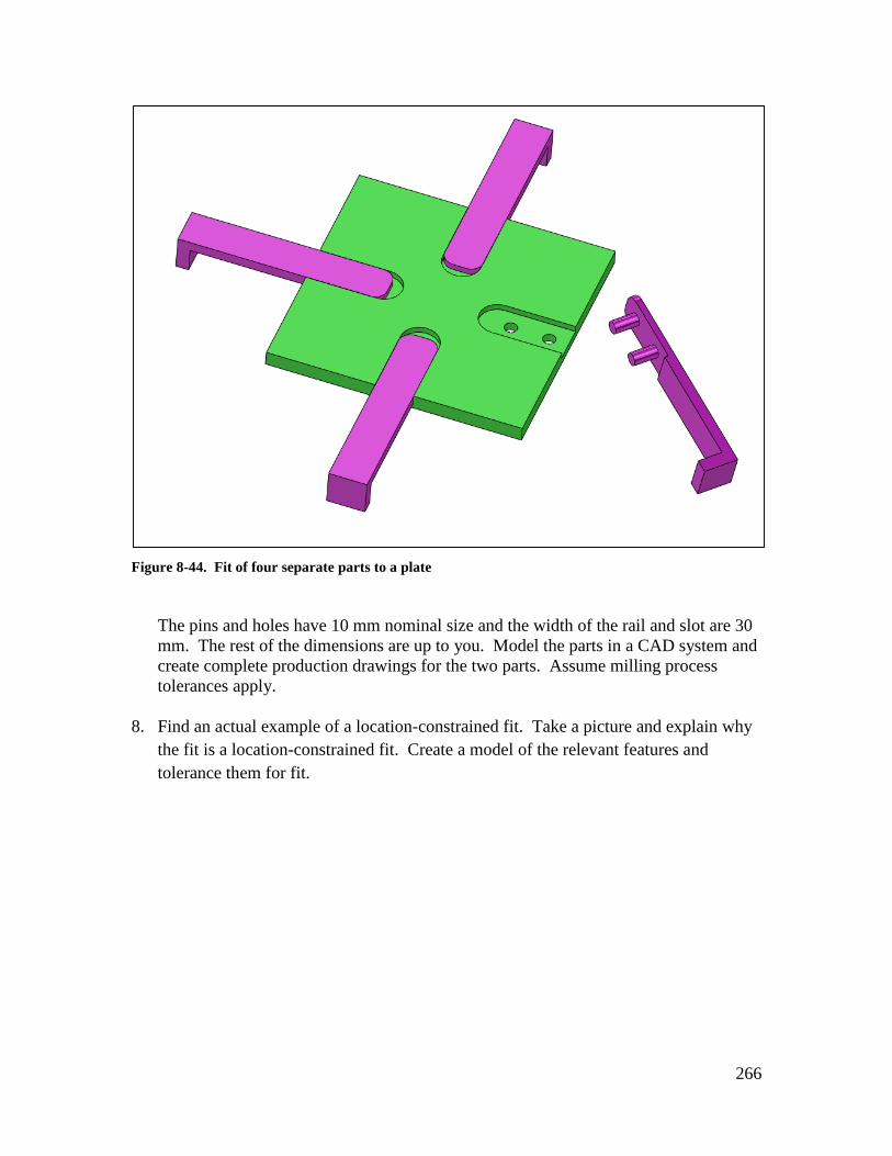
266

Figure 8-44. Fit of four separate parts to a plate

The pins and holes have 10 mm nominal size and the width of the rail and slot are 30

mm. The rest of the dimensions are up to you. Model the parts in a CAD system and

create complete production drawings for the two parts. Assume milling process

tolerances apply.

8. Find an actual example of a location-constrained fit. Take a picture and explain why

the fit is a location-constrained fit. Create a model of the relevant features and

tolerance them for fit.

267

Chapter 9 Assemblies with Threaded Fasteners

9.1. Overview

The fit analysis of general multipart assemblies will be presented in Chapter-11. The fit

of some common three-part assemblies, however, can be analyzed by extending the

methods presented so far for two-part assemblies. This chapter presents the formulas

needed to assure fit of some common three-part assemblies particularly fastener-related

assemblies including assembly with threaded studs and nuts, assembly with threaded

holes and screws, and assembly with loose bolts and nuts.

9.2. Fits using threaded studs or screws

Figure 9-1 shows a simple assembly of two plates with a threaded stud and a nut fitting a

clearance hole. In this example the pin is an integral part of the plate and is threaded.

This situation represents an assembly of two directly fitting parts. The figure shows a

single feature but in most cases it is a part of a pattern of features.

Figure 9-1. A two-part plate assembly with a threaded stud and a nut

To assure fit, the usual fit formula applies and the position tolerances can be obtained

from


The tolerancing scheme for this example is shown in Figure 9-2. In this chapter we will

use more realistic tolerance values.

268

10.50 – 11.09 9.5 – 10.1

A

B

A

B

Ø 0 A BMØ 0 A BM

10

30

Figure 9-2. Size and position tolerances necessary to assure fit

To find the size limits for the clearance hole, we select size limits that are consistent with

drilling tolerances. Drilling is often the process of choice for making fastener holes. In

this example, the designer can set up hole tolerances based on an 11 mm drill size. The

total size tolerance for this drilling operation is 0.09 mm. Drills are designed to create

holes that are at or slightly larger than their nominal sizes. Therefore instead of

specifying 11 ± 0.04 mm for the clearance hole size tolerance, we should specify a range

of 11.00 – 11.09 mm. When holes are intended to be created by other processes, it is

usually best to use symmetric size tolerance values around the nominal size. The fit

relationship is determined by the fit formula


Assuming equal position tolerances for hole and stud features and setting the MMC size

of the stud to be F=10 mm leads to

T = ½ (11 – 10) = 0.5

We can specify a position tolerance of TH = TF = 0.5 mm for both the clearance hole and

the stud. This position tolerance is well within the accuracy of the drilling process. It is

best, however, to specify a zero position tolerance specification for the clearance holes by

combining the position tolerance with the MMC size of the hole

H0 = 11 – 0.5 = 10.5 mm

The hole size limits become 10.5 - 11.09 mm. The combined size and position tolerance

for the hole is 0.59 mm.

When the size and position tolerance of the hole are specified separately, the equivalent

specification requires size limits of 11.00 – 11.09 mm and position tolerance of 0.5 mm.

For the stud, the size tolerance is assumed to be 0.1 mm. Using zero position tolerance

for the stud results in F0 = 9.5 mm. The LMC size of the stud becomes 10.1 mm. The

combined size and position tolerance for the stud is 0.6 mm.

269

9.3. Fits using threaded press-fit studs

Making metallic pins as integral parts of plates is difficult and costly. Machine designers

rarely design such features on metallic parts. Instead, plates are designed with holes to

which separate pins are press fitted. The more common design for the assembly of the

previous example looks as shown in Figure 9-3. This situation is similar to the assembly

of plates with threaded holes and cap screws. In fact, the stud and the nut together appear

like a screw.

8

10

Figure 9-3. A three-part assembly of two plates with a press-fitted threaded stud

The fit in this problem is no longer an assembly of two directly fitting parts. However,

there is a special tolerance specification that allows a designer to tolerance this assembly

as if the pin was an integral part of the plate it is pressed into. This special specification,

known as the projected tolerance zone, requires that the position tolerance statement be

applied not to the hole but to a pin of certain height inserted into the hole. The symbol

for the projected tolerance zone designation is a circled letter P. The letter P stands for

“Projected” but you may think of the symbol P to refer to “Pin”. This means the position

tolerance applies to a pin inserted into the hole and not the hole itself. During inspection,

real pins must be inserted into the holes and it is these pins that are the subject of the

position tolerance statement. The tolerance statements that assure fit in this case are

shown in Figure 9-4 for 12 mm fasteners with two unknown values to be determined.

270

??

12H7

A

B

A

B

Ø 0 A BM

Ø ?? 8 A BM P

8

10

Figure 9-4. Format of position tolerances and size tolerances necessary to assure fit

To assure a zero-clearance fit, the fit boundary of the clearance hole must be equal to the

fit boundary of the pin that is inserted into the stud hole

Hc,min + THc = Fmax + TF

Where Hc,min represents the MMC size of the clearance hole and Fmax is the maximum

size of the pin. THc is the position tolerance of the clearance hole. The fit formula is then

THc + THs ≤ Hmin – Fmax

TF is the position tolerance of the pin which is the same as the position tolerance of the

stud hole THs. When position tolerances for the clearance hole (THc) and stud hole (THs)

are selected to be equal, the formula becomes

TH ≤ ½(Hmin – Fmax)

This formula is called the fixed fastener formula and it also applies to plates fastened

together using cap screws and tapped holes. We can select a 12.5 mm drill for the

clearance hole and complete the specifications based on this drill size. The size tolerance

for drilling process for a 12.5 mm size clearance hole is 0.1 mm which results in size

limits of 12.5 – 12.6 mm. Using the fixed fastener formula, the position tolerance needed

to assure fit is

TH = THc = THs = ½ (12.5 – 12) = 0.25 mm

The position tolerance is well within the drilling position accuracy. We can specify

position tolerances of 0.25 mm for the clearance and stud hole. It is better to convert the

clearance hole specifications to zero position tolerance format by combining the hole

MMC size with the required position tolerance

H0 = 12.5 – 0.25 = 12.25 mm

The stud hole specification, however, cannot use the zero position tolerance format.

Figure 9-5 shows the complete specifications.

271

12. 25 – 12.60

12H7

A

BA

B

Ø 0 A BM

Ø 0.25 8 A BM P

8

Figure 9-5. Complete specifications for the assured fit of plates with a press-fit threaded stud

The treatment is exactly the same whether there is one fastener or a pattern of fasteners.

9.4. Assembly with cap screws and threaded holes

An alternative to press-fit studs and also a more common way of attaching two plates is

the use of cap screws and tapped holes. This situation is shown in Figure 9-6

8

Figure 9-6. Assembly of plates using threaded holes and cap screws

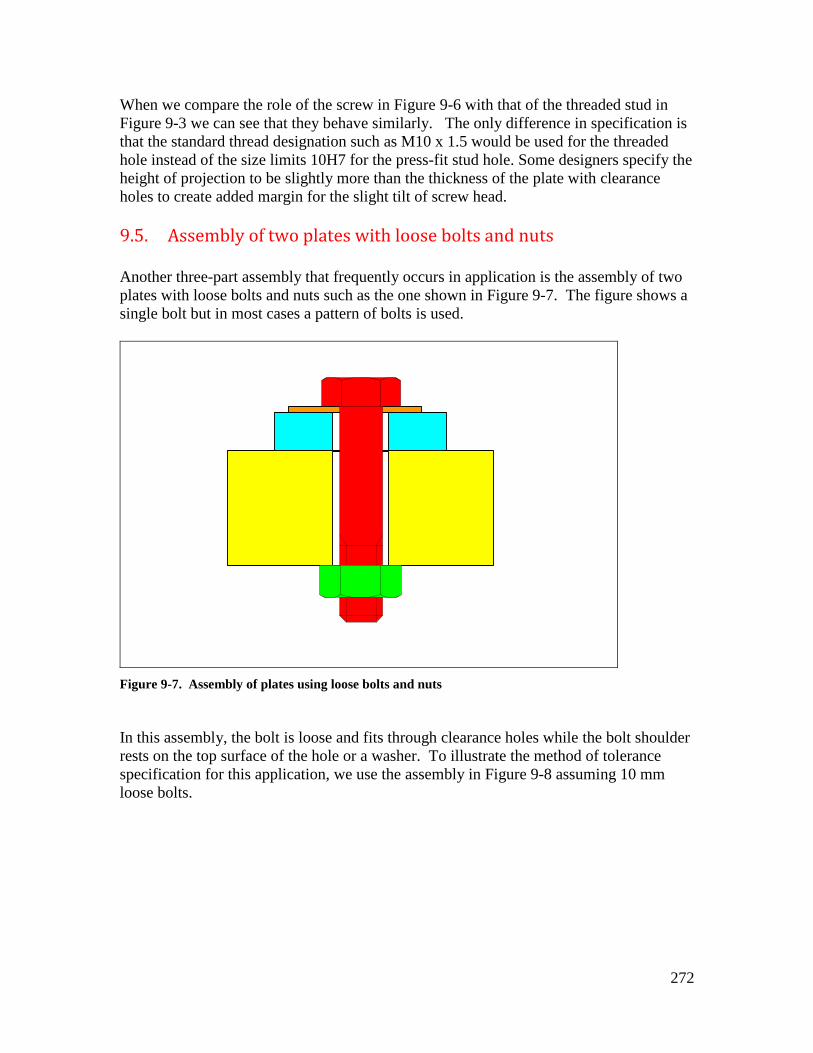
272

When we compare the role of the screw in Figure 9-6 with that of the threaded stud in

Figure 9-3 we can see that they behave similarly. The only difference in specification is

that the standard thread designation such as M10 x 1.5 would be used for the threaded

hole instead of the size limits 10H7 for the press-fit stud hole. Some designers specify the

height of projection to be slightly more than the thickness of the plate with clearance

holes to create added margin for the slight tilt of screw head.

9.5. Assembly of two plates with loose bolts and nuts Another three-part assembly that frequently occurs in application is the assembly of two

plates with loose bolts and nuts such as the one shown in Figure 9-7. The figure shows a

single bolt but in most cases a pattern of bolts is used.

Figure 9-7. Assembly of plates using loose bolts and nuts

In this assembly, the bolt is loose and fits through clearance holes while the bolt shoulder

rests on the top surface of the hole or a washer. To illustrate the method of tolerance

specification for this application, we use the assembly in Figure 9-8 assuming 10 mm

loose bolts.

273

Figure 9-8. Plates fastened together using a pattern of loose bolts and nuts

The assembly of the bolts with clearance holes in the two plates creates a three-part

assembly for which we need to use a more general tolerance analysis method in order to

derive the fit formula. This more general analysis method would be presented later in

Chapter-11 on tolerance analysis. The result of the analysis is shown in the following fit

formula:

TH1 + TH2 ≤ (H1min – Fmax) + (H2min – Fmax)

In this formula, TH1 and TH2 are the position tolerances of the clearance holes, H1min and

H2min are the MMC sizes of the clearance holes, and Fmax represents the fit boundary of

the bolt which is usually its maximum shank diameter. Clearance holes often have

identical specifications leading to the more common formula

TH ≤ Hmin – Fmax

This formula is called the floating fastener formula. A direct comparison with the fixed

fastener formula, TH ≤ ½(Hmin – Fmax), indicates that the clearance hole position

tolerance values for floating fasteners can be twice as large as those for the fixed fastener

case. This is because a loose bolt can relocate itself (or float) in the existing opening

between the two plate holes while a fixed fastener is rigidly attached to the threaded hole

or press-fitted into a plate.

Although the calculations are simple, the fastener applications are so common that

automating the process is worth the effort. The FAP (Fastener Application Program) is a

simple version of such a program. Figure 9-9 shows the dialog window that accepts the

input paramenters and suggests a solution for a fastener problem. The fastener size is 12

mm.

274

Figure 9-9. The dialog window of FAP showing the input parameters and the results

On the left-hand side is the fastener size and the minimum and maximum size of the hole

associated with the hole-making process. In this case the process size limits are

associated with a 12.5 mm drill. The manufacturing accuracy program (MAP) can be

used to determine realistic size limits for drilled holes and an estimate of the position

tolerance of the process. The process position tolerance, in this case 0.3 mm, would be

used to check whether the chosen parameters assure free fit. The results show that the

tolerance specifications do not assure fit for the fixed fastener case. This is because the

required tapped hole position (0.25 mm) is smaller than the indicated 0.3 mm process

tolerance. In this case we can increase the size of the drill to achieve a fit. For the

floating fastener application the assembly is assured. When the fit is assured, it is also a

good practice to try a smaller size drill to check if a better fit can be achieved. For

example if initially a 13 mm drill is selected, the maximum fit gap would be 1.1 mm.

Checking a 12.5 mm drill results in a better fit without additional costs. FAP uses equal

position tolerances for all clearance holes.

9.6. Fastener applications - Example-1

Consider the offset arm assembly in Figure 9-10 in which two identical parts called arms

fit a base plate with four cap screws. We are asked to specify the size and position

tolerance of the clearance holes separately and not use zero position tolerance format.

275

Figure 9-10. The offset arm assembly

The arm and the base plate must fit together with standard M10 screws while the seating

surfaces are in full primary contact and the locating edges are in secondary contact. The

depth of the clearance holes as well as the tapped holes is 10 mm.

We first check the specifications for 10.5 mm drills. The size tolerance to be used with a

10.5 mm drill hole is 0.1 mm which will be divided as 10.49 – 10.59 mm to provide a

little extra margin for worn out drills. We can check the fit using the fixed fastener

formula

THc + THt ≤ Hmin – Fmax

In this case

Hmin – Fmax = 10.49 – 10 = 0.49 mm

Therefore

THc + THt = 0.49 mm

We can divide the total position tolerance between the clearance and threaded hole and

use 0.24 mm for each. The arm tolerances related to this fit are shown in Figure 9-11.

276

Figure 9-11. Arm tolerances

The pattern of two holes can shift up or down with more allowance because that

relationship is not precision and its control is left to the default tolerances. The tolerances

for the plate is shown in Figure 9-12.

277

Figure 9-12. The SEP REQT designation means there are two patterns of two holes with separate fit

requirements.

The patterns of two holes are treated separately because they fit to two separate parts.

This is indicated by the note SEP REQT written beneath the tolerance control statement.

This means that the two patterns of holes are gaged separately with two-hole gages rather

than as one pattern of four holes. The result is that the distance between the two patterns

is not controlled with precision. The GDT standard states that if two or more position

tolerance statements use exactly the same datum frame for multiple feature patterns, the

patterns are considered to be a single pattern unless SEP REQT is indicated.


Consider the blade and the blade holder assembly shown in Figure 9-13. This fit problem

involves one primary orienting surface (seating surface), one secondary orienting and

locating surface (back surface), one width feature fit (blade width) and a pattern of screw

fits. The threaded holes in the blade holder accept 8-mm cap screws.

278

Figure 9-13. Blade and blade holder

The blade and the blade holder must fit together and get fixed with standard screws while

the seating surfaces are in full primary contact and the back surfaces are in secondary

contact. The fastener holes are intended to be drilled. We like to set up the tolerances for

a fit with a maximum gap of 0.5 mm in the blade to blade holder width fit.

The blade width feature and the blade holder have an orientation-constrained fit. Using

zero-perpendicularity tolerance for both features and a fit boundary of 140 mm, we get

H0 = F0 = 140 mm

Using the maximum gap size of 0.5 mm and equal size tolerances on both width features

leads to

Hmax = 140.25 mm

Fmin = 139.75 mm

The size tolerances are well within machining process capabilities. For the fit of cap

screws we select a 8.5 mm drill size for clearance holes. For a 8.5 mm drill size the total

size tolerance of 0.08 mm is attainable. The clearance hole size limits will be specified as

8.5 mm to 8.58 mm. For the fit of cap screws we use the fixed fastener formula


With Hmin = 8.5 mm and Fmax= 8.0 mm, the total position tolerances must be

THc + THt ≤ 0.5 mm

Using equal position tolerances for both tapped and clearance holes, we can select

THc=0.25 and THt = 0.25 mm. These position tolerances are within the positioning

accuracy of the drilling process. We can also convert the clearance hole specifications to

zero-position tolerance by expanding the hole size limits on the MMC side. For the

clearance holes, the zero position MMC size limit becomes (H0 = 8.5 – 0.25 = 8.25 mm)

while the LMC limit remain as 8.58 mm.

279


The use of alignment pins is a common method of locating and orienting two parts with

respect to each other. In this method the alignment features can be placed at the edges of

parts leaving the middle for bearing holes or other functional features. Figure 9-14

shows a simple two-part gear housing assembly in which the center bearing holes are

aligned with precision by locating them relative to two alignment pins and holes. Other

functional features of the two parts such as gear pin holes are not shown to focus on the

fastener application. The primary manufacturing process is die casting for these

aluminum parts. The alignment pins are cast as integral parts of the housing piece.

Figure 9-14. Gearbox housing

The physical assembly used for this example is shown in Figure 9-15.

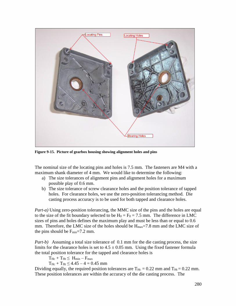
280

Figure 9-15. Picture of gearbox housing showing alignment holes and pins

The nominal size of the locating pins and holes is 7.5 mm. The fasteners are M4 with a

maximum shank diameter of 4 mm. We would like to determine the following:

a) The size tolerances of alignment pins and alignment holes for a maximum

possible play of 0.6 mm.

b) The size tolerance of screw clearance holes and the position tolerance of tapped

holes. For clearance holes, we use the zero-position tolerancing method. Die

casting process accuracy is to be used for both tapped and clearance holes.

Part-a) Using zero-position tolerancing, the MMC size of the pins and the holes are equal

to the size of the fit boundary selected to be H0 = F0 = 7.5 mm. The difference in LMC

sizes of pins and holes defines the maximum play and must be less than or equal to 0.6

mm. Therefore, the LMC size of the holes should be Hmax=7.8 mm and the LMC size of

the pins should be Fmin=7.2 mm.

Part-b) Assuming a total size tolerance of 0.1 mm for the die casting process, the size

limits for the clearance holes is set to 4.5 ± 0.05 mm. Using the fixed fastener formula

the total position tolerance for the tapped and clearance holes is


THc + THt ≤ 4.45 – 4 = 0.45 mm

Dividing equally, the required position tolerances are THc = 0.22 mm and THt = 0.22 mm.

These position tolerances are within the accuracy of the die casting process. The

281

combined size and position tolerance for the clearance holes to be used with zero-position

tolerance format becomes 4.23 – 4.55 mm. This is obtained by expanding the clearance

hole size limits of 4.45 – 4.55 mm on the MMC side by 0.22 mm.

The tolerancing of the part with alignment pins is shown in Figure 9-16. The flatness

value of 0.3 mm for the primary datum is chosen to be consistent with the die casting

process and is considered acceptable for this slow-speed low cost gearbox.

Figure 9-16. Tolerances for the part with locating pins

The tolerancing of the part with the alignment holes looks very similar to the part with

pins. Figure 9-17 shows the tolerancing of the part with alignment holes and threaded

holes.

282

Figure 9-17. Tolerances for the part with locating holes and threaded holes


The assembly of the two parts shown in Figure 9-18 is to be toleranced for fit. The part

with the center pin is the base and the part with the center hole is the socket. There is a

center feature fit for radial alignment and a dowel pin fit for rotational alignment of the

two parts. Screws are used to rigidly fix the parts together.

283

Figure 9-18. The base and socket are aligned using a center cylindrical fit and a dowel pin

The primary orientation between the two parts is fixed through the seating surface

contact. The parts are located precisely with respect to each other through the alignment

boss and hole in the center of each part. The in-plane orientation between the two parts is

set by a dowel pin that is pressed into the base hole and fits the socket hole. Fixed

fasteners are then used to fix the two parts together.

The nominal size of the center fit feature is 20 mm, the dowel pin is 5 mm, and the

fasteners are M5. The thickness of the socket plate is 10 mm. The final processes are

machining. We need to tolerance the two parts for the following requirements:

a) The center fit between the boss and the hole must not allow a play of more than

0.1 mm.

b) The dowel pin must fit tightly into the base with a slight interference.

c) The play in the dowel pin fit must not exceed 0.25 mm

d) The two parts must align sufficiently to allow M5 fasteners to fix the parts.

Part-a) Using the zero-geometric tolerance method, the size limits of the boss should be

set to 19.95 – 20.00 mm and the size limits of the center hole should be set to 20.00 –

20.05 mm. Both features will have a zero perpendicularity tolerance at MMC

specification. The primary datum is the seating surface (datum-A) and its flatness is

controlled to 0.05 mm consistent with the milling process and sufficient to prevent

rocking. Figure 9-19 shows the result for the base after this step.

284

Figure 9-19. The base tolerances to achieve precision center boss and hole fit

Part-b) The size limits of the press-fit hole receiving the dowel pin is specified to be 5H7

to fit a dowel pin of size 5p6 for a tight locational interference fit.

Part-c) The fit of the dowel pin to the clearance hole in the socket is a fixed fastener fit

case. Using the fixed fastener formula

THc + THp ≤ Hmin – Fmax

Hmin is the MMC size of the clearance hole, Fmax is the MMC size of the dowel pin, and

THc and THp are the position tolerances of the clearance and press-fit holes respectively.

We will use the tolerances associated with precision drilling operations and then check to

make sure the fit play will not exceed the stated 0.25 mm. The total size tolerance for a

5.2 mm drill is 0.05 mm. We will set the size limits of 5.20 – 5.25 mm for the hole

created by this drill. Using the fixed fastener formula

THc + THp ≤ Hmin – Fmax = 5.2 – 5 = 0.2 mm

Dividing this position tolerance equally between the clearance hole and press-fit hole

THc = 0.1

THp = 0.1

These position tolerances are within the capability of precision drilling process. We can

now check the maximum play in the dowel pin fit.

285

The maximum play in the dowel pin fit is


Pmax = 5.25 – 5.0 = 0.25 mm

The maximum play is equal to the required limit of 0.25 mm. We can covert the

clearance hole limits to zero position format by expanding the size limits to 5.10 – 5.25

mm. Figure 9-20 shows the result for the base part with press-fit holes after setting up

the dowel pin fit.

Figure 9-20. The base tolerances to achieve precision dowel pin fit

Part-d) The fastener holes for M5 screws can be created by 5.5 mm drills holding size

limits of 5.50 – 5.58 mm. Using the fixed fastener formula

THc + THt = Hmin – Fmax

THc + THt = 5.5 – 5.0 = 0.5 mm

Dividing this total position equally between the threaded and the clearance holes leads to

THc = THt = 0.25 mm. The position tolerance is directly applied to the threaded holes.

With the clearance holes, we use the zero position size limits by expanding the clearance

hole size tolerance by 0.25 mm on the MMC side to obtain 5.25 – 5.58 mm. The

complete tolerance specifications related to the required fits are placed on the base part

drawing as shown in Figure 9-21.

286

Figure 9-21. Complete size and position tolerances for the fit of all features

Note that both the dowel pin holes and threaded holes require the projected tolerance

zone specification. Figure 9-22 shows the complete tolerancing of the socket part.

287

Figure 9-22. Complete tolerancing of the socket part

9.10. Tolerance design of press-fit inserts

The simple assembly shown in Figure 9-23 is similar to a two-part orientation-

constrained fit except that one of the parts has a press-fit insert.

Figure 9-23. Assembly of a hole feature with a press-fit insert

288

The part that accepts the insert is toleranced as shown in Figure 9-24. Note that the

MMC modifier cannot be used on the perpendicularity of the hole because the hole

requires precise size control for press-fit application.

Ø 0.1 A

25H7

0.05

A

Figure 9-24. The hole precision size tolerance is necessary for the press-fit insert

The insert and the plate with the boss are toleranced in Figure 9-25. The outer diameter

of the insert fits the plate hole with a light interference fit. The inner diameter must be

controlled to be parallel to the outer diameter. In this simple three-part assembly, the

location of the inner diameter with respect to the outer diameter is not important because

the top part is loose and can center itself to line up with the boss.

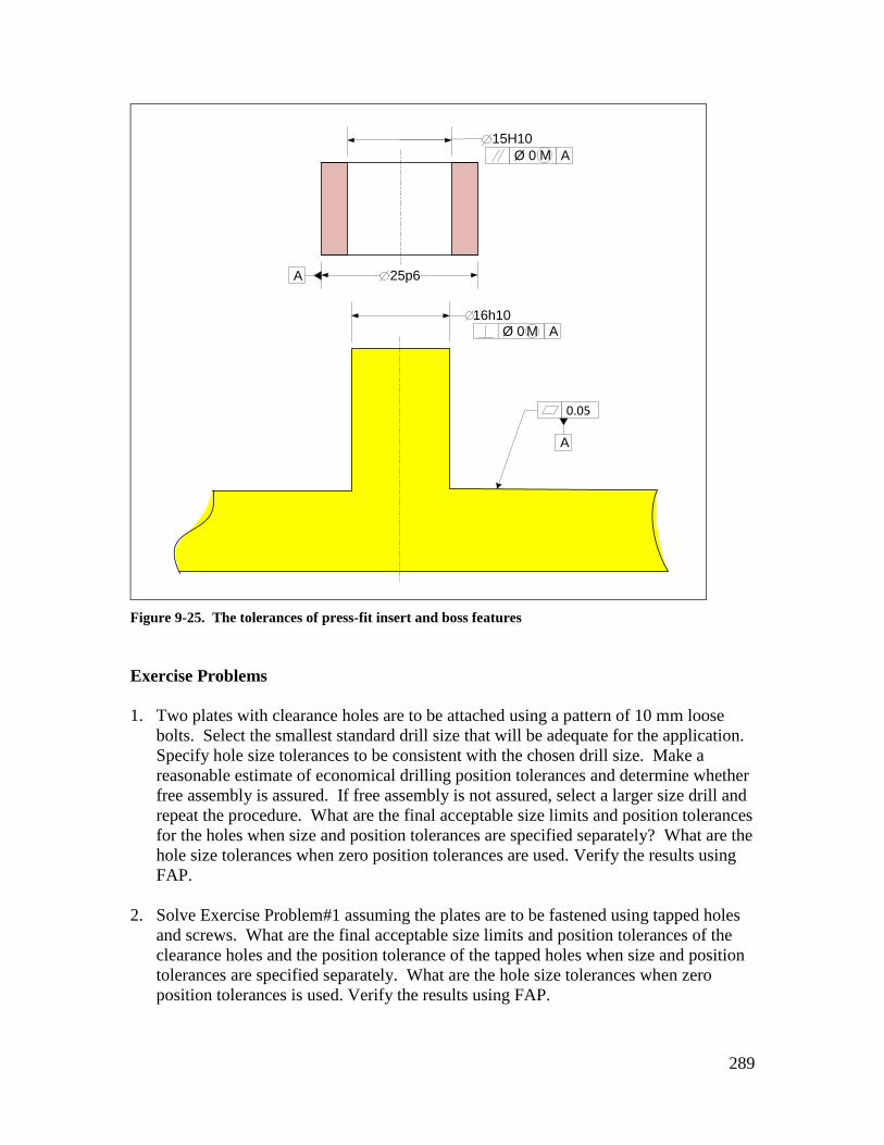
289

15H10

A 25p6

Ø 0 AM

A

16h10

Ø 0 AM

0.05

Figure 9-25. The tolerances of press-fit insert and boss features

Exercise Problems

1. Two plates with clearance holes are to be attached using a pattern of 10 mm loose

bolts. Select the smallest standard drill size that will be adequate for the application.

Specify hole size tolerances to be consistent with the chosen drill size. Make a

reasonable estimate of economical drilling position tolerances and determine whether

free assembly is assured. If free assembly is not assured, select a larger size drill and

repeat the procedure. What are the final acceptable size limits and position tolerances

for the holes when size and position tolerances are specified separately? What are the

hole size tolerances when zero position tolerances are used. Verify the results using

FAP.

2. Solve Exercise Problem#1 assuming the plates are to be fastened using tapped holes

and screws. What are the final acceptable size limits and position tolerances of the

clearance holes and the position tolerance of the tapped holes when size and position

tolerances are specified separately. What are the hole size tolerances when zero

position tolerances is used. Verify the results using FAP.

290

3. The slot feature of the turning support is to fit to the rail of the base and be fixed to

the base using a 12 mm loose bolt. Figure 9-26 shows the turning support.

Figure 9-26. Turning support

We like to create the necessary tolerance statements for the fit of the slot and rail as well

as a 12 mm loose bolt. The play in the slot and rail fit should not exceed 0.1 mm. The

bolt holes are to be drilled.

4. Consider a plate with six clearance holes fitting a plate with six threaded holes using

10 mm cap screws as shown in Figure 9-27. The center boss has a nominal size of 40

mm and fits a center hole on the mating part. The maximum play in the center fit is

to be 0.1 mm. The clearance holes for the screws are to be created by drilling. The

thickness of both plates is 8 mm. Model the assembly on a CAD system and fully

tolerance the two parts for proper fit.

291

Figure 9-27. Assembly of two plates using a pattern of cap screws

5. Find an actual example of the assembly of two parts with floating fasteners. Take a

picture and using a simple drawing indicate the specification types necessary to

achieve a fit.

6. Find an actual example of the assembly of two parts with fixed fasteners. Take a

picture and using a simple drawing indicate the specification types necessary to

achieve a fit.

7. Consider the post-holder and base plate shown in Figure 9-28. A partially

dimensioned drawing of the post holder is shown in Figure 9-29. A lip on the

mounting surface of the post-holder fits tightly into the base part. The four clearance

holes are to align with tapped holes in the base for M8 cap screws. Use the size limits

of 50 H9 and 50d9 for the lip fit features. Both parts are to be made by machining.

Create a model of this assembly along with fully dimensioned and toleranced

drawings of the parts.

292

Figure 9-28. Assembly of post holder and base plate using a pattern of cap screws

Figure 9-29. A partially dimensioned drawing of the post holder

293

Accuracy of Manufacturing Processes (MAP) Program

Estimates of drill tolerances can be obtained from the Manufacturing Accuracy Program

(MAP). The dialog window shown in Figure 9-30 represents a sample input for a drill.

The user selects the drill size, the depth of the drilled hole, and whether the drilling

process is performed with high or regular degree of accuracy.

Figure 9-30. The size accuracy of the drilling process

In this case, the user has selected to estimate the size tolerance for a 11 mm drill and the

answer is in the ± format. The total size tolerance is about 0.09 mm. The position

tolerance for this drilled hole is shown in Figure 9-31.

294

Figure 9-31. The position accuracy of the drilling process

295

Chapter 10 Tolerance Design of Multipart Fits

10.1. Overview

In the previous chapters we discussed the tolerance design and tolerance analysis for fits

involving two parts. Simple formulas were developed to assure fit between two directly

fitting parts using the concept of fit boundaries. We also looked at the case of two parts

fixed together by fasteners.

In multipart fits, a fit is influenced by the dimensions and tolerances of more than two

parts. The collection of part dimensions often forms a loop with each part connecting to

two other parts in the loop. Fit ability becomes the result of how the tolerances

accumulate or stack up in the worst case situations. For that reason, tolerance analysis is

sometimes called stack analysis. If the tolerances accumulate to a value greater than the

clearance allocated by the design, the parts may not fit together. Design engineers often

try to avoid precision fits that depend on more than two parts. When that is unavoidable,

designers try to minimize the number of parts and features that influence a precision fit.

Obviously, the more the number of tolerance values that influence a fit, the smaller each

tolerance value needs to be to achieve that precision fit.

The rules and preferences for tolerance design (synthesis) are intuitive but do require

practice. Tolerance analysis procedure for multipart fits is more mathematical. For that

reason, tolerance design and tolerance analysis are presented in separate chapters.

Tolerance design is the more important step and requires the selection of best tolerance

types. This chapter presents the preferred practices for tolerance design of multipart fits.

Tolerance design for fit requires a designer to first recognize the parts, features, and

geometric deviations that influence a fit. Subsequently proper types of tolerances should

be applied in a manner similar to what was done for two-part fits. Initial tolerance values

should be selected based on processes that the designer believes would produce the

required precisions. An estimate of these tolerance values can be obtained using the

Manufacturing Accuracy Program (MAP). The initial dimension and tolerance values

applied to parts may not assure fit or may not be the best choices. Tolerance analysis,

which follows tolerance design, will allow a designer to adjust the initial dimensions and

tolerance values to achieve the desired fit performance. The fit performance refers to the

minimum and maximum possible values of a critical gap or dimension.

This chapter presents the tolerance design methodology and preferred practices using a

variety of example problems. It is important to study all of these examples because they

cover many kinds of assemblies. Most of the examples are set up as simple geometric

constructions rather than real machine assemblies. This is done intentionally to focus on

specific concepts and to reduce distractions.

296

10.2. Application of profile tolerances

Example-1: A simple tolerance design problem: A simple assembly is shown in Figure

10-1. Assume the parts are three dimensional and have depth. The gap between the end

surfaces of part2 and part3 is a critical assembly dimension and must not become

negative. None of the dimensions of part1 influence the gap. The flatness of the top

surface of part1 is the only important geometric aspect of part1 influencing the gap. The

figure shows the dimensions influencing the gap as vectors. Each vector belongs to a

single part except for the gap vector that jumps across the gap between two parts. We

will see the use of vectors for mathematically representing dimensions and tolerances in

Chapter-11 on tolerance analysis.

The vectors establish a theoretically common orientation along which the distances

influence the gap. Some tolerance statements control the size of the vectors along the

common orienting direction while other tolerances control the direction of some vectors

to closely align with the common orienting direction. The common orienting direction is

determined by the surfaces that orient the parts with respect to the assembly. In the case

of this simple problem the common direction is perpendicular to the top surface of part1.

gap

part1

part2

part3

Figure 10-1. An example of a fit involving two dimension values

For this problem, the gap is influenced by one dimension on each part. Figure 10-2

shows how the relevant features are initially toleranced to control the critical gap. In this

case, profile tolerances are used for dimension control. Datum control statements are

shown in red while the dimensions that directly influence the gap are shown in black.

Tolerance values are to be selected based on the processes believed to have sufficient

precision to meet the requirements. Theoretical dimensions and sizes are initially

selected to allow a small gap. The tolerance analysis procedure, which will be presented

in Chapter-11, will adjust the initial theoretical dimensions and, if necessary, the

tolerance values such that the gap requirements are met.

297

A A

0.1 A

50

0.1 A

51

0.05 0.05

Figure 10-2. Profile tolerances control the fit gap in the example

In tolerancing multipart fits it is helpful to define a presumed order of assembly. The

presumed order of assembly is just an organizational tool to make tolerancing practice

easier and more uniform among designers. The presumed order of assembly need not

match the actual order of assembly for the tolerancing to be correct. The part numbers in

these examples identify the presumed order of assembly.

In this chapter we will use convenient tolerance values but in real assemblies realistic

tolerance values must be used. Datum precision tolerances, i.e. the flatness statements,

are shown in red while direct fit-related tolerances are shown in black.

Many fit applications involve the geometric accuracy of more than two parts. These fits

are referred to as multipart fits. The following example is a multipart fit that needs

mainly profile tolerance specifications.

Example-2: A simple four-part tolerance design problem: Figure 10-3 shows a simple

four-part assembly in which all four parts influence the gap value. The gaps as well as

the vectors representing various dimensions are also shown.

298

G

Aa

Fa

Ca

Da

1 2

3 4

Figure 10-3. An example of a fit involving four parts

The tolerancing of part1 is shown in Figure 10-4. Only the tolerance statements relevant

to the gap control are shown. Datum-A orients the part with respect to the rest of the

assembly. We can also select the top surface as the part orienting datum. Given two

equally valid options we use the presumed order of assembly to make the selection. In

this case, the lower surface contacts part1 first according to the presumed order of

assembly.

A

50.1 A 0.05

0.06 A

Figure 10-4. Tolerancing of part1 in the example assembly

The top surface controls the orientation of part3 or vector Da. The parallelness

specification is necessary to minimize the angular deviation of this vector from the

common orientation direction. The parallelness statement minimizes the distortion angle

between part2 and part3. Distortion control specifications are shown in green. The profile

299

specification controls a dimension that directly influences the main fit. The reference to

datum-A in the profile statement indicates that measurements must be made along the

common orienting direction. The tolerancing of part2 is shown in Figure 10-5.

5.0 – 5.1

0 M

0.05A

0.06 A


Datum-A establishes the orientation of this part with respect to the assembly. The top

surface can also be chosen as the orienting datum but the selected datum-A occurs first

according to the presumed order of assembly. The height of the plate influences the main

gap directly and is controlled by size limits. This dimension can also be controlled by a

profile tolerance but size limits are preferred. The parallelness specification is necessary

to minimize the angular deviation of vector Aa from the common direction. The

parallelness specification minimizes the angular distortion between part1 and part4. The

tolerance specification of part3 is shown in Figure 10-6. Datum-A is the primary

orienting surface for this part.

300

A

0.1 A

51

0.05


The tolerancing of part4 is shown in Figure 10-7.

A

0.1 A

50

0.05


301

10.3. Fits involving features-of-size

Example-3: A simple four-part fit: Consider the assembly shown in Figure 10-8. To

simplify the parts, assume that part2 and part3 are glued to part1.

part1

part2 part3

part4

Figure 10-8. A four-part assembly with two fit features

The glued surfaces are indicated in the figure in thick red lines and define the primary

orienting direction. Part4 is expected to slide in and fit through the opening and rest on

the two surfaces that form a ledge. The tolerance design for the four parts is shown in

Figure 10-9.

302

A

100 – 100.1

Ø 0 AM

A

A

B

5

0.1 A B

100.1 – 100.2

Ø 0 AM

0.05

0.05

0.05

0.08 A

part1

part4part2

A

0.05 A

Figure 10-9. The initial assignment of dimensions and tolerances

Part1 contacts part2 and part3 on the same surface. This surface is selected as datum-A on

part1 and its flatness is controlled. The datum-A surface is the primary orienting feature

for this part. The width dimension is the dimension that directly influences the gap.

The primary orienting surface for part2 is datum-A. The profile tolerance with tolerance

value of 0.1 mm controls the dimension that directly influences the gap. Note the use of

the primary orienting datum in the profile statement. The profile tolerance with 0.05

tolerance value is specified to align the two seating surfaces and create a horizontal

support surface for part4. This precision is necessary to create a stable contact and is a

function-related specification. Function-related specifications are shown in blue.

The primary orienting surface for part4 is datum-A. The width dimension of this part

directly influences the gap.

Example-4: Retaining ring fit on a gearbox shaft: One of the main applications of

tolerancing is in the axial placement of power transmission components on shafts. One

of the simplest examples of fit involving three parts is a gear that is axially constrained by

a shaft shoulder on one side and a retaining ring on the other as shown in Figure 10-10.

303

Figure 10-10. A gearbox shaft with a retaining ring fixing the axial location of the gear

The gear and the retaining ring are purchased parts. We need to determine the

specifications for the shaft groove size and its location for the retaining ring to fit the

space between the groove and the gear. In addition, the ring must limit the gear play to a

specified maximum value. Figure 10-11 shows a larger view of the relevant features.

part1

part2

part3

gap

Figure 10-11. The retaining ring limits the axial play of the gear

The gap of interest is the distance between the gear face and the retaining ring face.

The initial dimensions and tolerances that control the gap are shown in Figure 10-12.

The dimensions and tolerances for the gear and the retaining ring are provided by the

manufacturer. The retaining ring groove size is selected to be slightly larger than the ring

with a size range of 1.04 - 1.14 mm. The groove center plane location is not directly

304

controlled by a position tolerance. Instead, a profile tolerance is used to directly control

the functional right edge of the groove.

B

30 +/- 0.05

1 +/- 0.02

31.5

1.04-1.14

0.05

Purchased Parts

A

0.05 A B


Usually slots and grooves are controlled by size and position but this is a special situation

in which only the right edge of the slot plays a precision role. For that reason, only the

right edge is controlled with precision using a profile tolerance.

What feature primarily orients the shaft with respect to the assembly? For a shaft with

bearing fits at the two ends, the orienting features are always the bearing fit surfaces. In

Figure 10-12 only one bearing fit is shown and that bearing fit surface is selected as the

primary orienting datum. The profile statement requires that the measurements be made

from the shoulder (datum-B) in the direction defined by the bearing fit (datum-A).

Example-5: Thermal expansion gap of a gearbox shaft: Figure 10-13 shows the

gearbox shaft assembly that was shown before. The figure also shows the dimensions

that influence the gap identified in the figure. The gap between the housing and the

bearing outer face on the left side bearing is a critical dimension that determines the axial

free play of the shaft. This axial free play accommodates the thermal expansion of the

305

shaft and reduces the precision requirements of the shoulder-to-shoulder distance. If the

gap is too small, the bearings may get axially loaded when the shaft heats up, or when the

shaft is not made with high precision. If the gap is too big the gears may not align

precisely enough due to excessive axial misalignment.

F1 F2

C

gap

part1

part2

part3

part4

part5

B

F3

Figure 10-13. The gap dimension in this gearbox depend on six part dimensions

Figure 10-14 shows the initial assignment of tolerances that control the gap dimension.

The theoretical dimensions, which are not shown, can be set up to create a small initial

gap. Tolerance analysis can then adjust the selected initial values to obtain the required

gap range. The primary orienting datum for the shaft is defined by the two bearing fit

surfaces.

306

100.0 – 100.2

A

A

A

0.05 A

0 AM

0.05

Ø 0.05

10 f7 10 f7

B

A-B

0.05 A

B

B

0.08 A B

0.08 A

1

3

5

Figure 10-14. The initial assignment of tolerances

The pair of functional shoulders of the shaft is considered to be a feature-of-size and its

size is controlled by direct dimension limits. Note that the perpendicularity tolerance

allows a maximum of 0.2 mm tilt with respect to the axis of rotation when the distance

between the shoulders is at the LMC limit of 100 mm. This amount of tilt may be

objectionable as the shoulders control the alignment of the bearing races. We can keep

the specifications for fit and function separate and add a new circular runout statement to

keep the bearing support shoulders perpendicular to the axis of rotation (datum-A) with

higher precision than 0.2 mm.

The orienting feature of part5 is the shoulder designated as datum-A. If the fit of the

cylindrical surface is tight, the cylindrical surface (datum-B) can be selected as the

primary orienting feature. In some situations it is not clear which surface will be the

primary orienting feature. In such cases the designer would select one of the features as

307

the primary orienting feature but adds tolerance statements that create a precision

relationship between the two surfaces. Figure 10-15 shows how the tolerancing would

change if we pick the cylindrical fit surface (axis) as the primary orienting datum.

B

A

0.05 A

0.08 A B

5

Figure 10-15. Tolerancing of part5 if the cylindrical surface is selected as the primary orienting

datum

The profile statement requires the measurements to be from datum-B in the direction of

the datum-A axis.

The primary orienting feature of part1 is the bearing fit surfaces designated as datum-A.

The datum-B must also be controlled to be perpendicular to datum-A with high precision.

This is achieved by a perpendicularity tolerance.

Example-6: A multipart tolerance design with loose fit features

Figure 10-16 shows a three-part assembly. The main gap is influenced by the play in the

loose slot and rail fit. The slot and rail fit may also be a hole and boss fit. We would like

to set up the dimensions and tolerances to assure a minimum main gap of zero.

308

part1

part3

part3

part2

Main gap

Figure 10-16. A multipart assembly with loose fit features

We start with the tolerance requirements of part1. There are two objectives in tolerancing

the slot in part1. First, the slot has an orientation-constrained fit to the rail of part3.

Figure 10-17 shows the tolerance statements necessary to meet this first objective. Based

on this specification, the largest slot can be 20.1 mm wide. The figure also shows a 30

mm theoretical distance of the slot center plane with respect to the left edge.

A

0 AM

20.0 – 20.1

300.05

Figure 10-17. Tolerancing of part1 for direct fit to rail

The second objective in tolerancing the slot is to limit the slot influence on the main gap.

As a general rule, whenever a loose fit feature, such a slot and rail fit, is in the path of the

main gap and the loose fit can be adjusted to a favorable arrangement during assembly,

the position tolerance is best to be qualified with an m modifier. We have seen many

examples for two-part fits that use the m modifier because in two-part fits we can always

find the most favorable arrangement for one part snapping into another. To further

explain this rule, when the slot is at its MMC limit of size (smallest slot) we have

309

minimum amount of slack to take advantage of during assembly and therefore we would

like to limit the feature center plane deviation at MMC. If the slot is made to be larger

than its MMC limit of size, we can allow more position deviation because the larger slack

allows us to compensate for its additional deviation during assembly. Sometimes

designers intentionally design large slacks in some fits when it is possible to exploit the

slack at assembly time.

When the final arrangement of the loose fit is unpredictable during assembly, the position

tolerance of the slot is better to be modified with an l modifier. In such a case, a slot

that is at or near its LMC limit of size presents the worst size for the slot as it allows the

most misalignment of center planes. A slot closer to its MMC size allows less slack and

it becomes the better size for fit.

For this example, Figure 10-18 shows an arrangement of the loose features that is

favorable to fit in the main gap. This is because the part has been pushed in a direction

that maximizes the main gap and allows the fit to happen. If we can assure this

arrangement during assembly we should use the m modifier.

Figure 10-18. The arrangement of the loose parts that is most favorable to fit related to main gap

When the final arrangement is unpredictable, the worst situation for fit may occur as

shown in Figure 10-19. For example, this arrangement may be bolted down in this

manner before the next part is inserted. In such cases it is best to use the l modifier. To

avoid confusion, remember the following rules:

1. If a fit feature is in the path of the main fit and its final arrangement is

unpredictable during assembly, use the l modifier for its positioning. Also use

the l modifier when such a feature is referenced as a datum.

2. If a fit feature is in the path of the main fit and its final arrangement is subject to

favorable manipulation during assembly, use the m modifier for its positioning.

Also use the m modifier when such a feature is referenced as a datum.

3. Always use the m modifier for the main fit features themselves.

310

Figure 10-19. The arrangement of the loose parts that is least favorable to fit related to main gap

In this example, we assume that the final arrangement of the slot and rail fit is

unpredictable. Figure 10-20 shows the final tolerance specifications for the slot. The

primary orienting surface with respect to the assembly is datum-A.

A

20.0 – 20.1

40

B

0 AM

0.3 A BL

0.05

0.08 A

1

Figure 10-20. Tolerances of part1 and the slot assuming the final arrangement of the slot fit is

unpredictable during assembly

Note that the 0.1 mm represents the combination of size and perpendicularity tolerance.

Since orientation control can be done with higher precision than location control with the

same process, it is appropriate to use a non-zero position tolerance. In this case, each

statement is related to a different fit.

Figure 10-21 shows the tolerance specifications for part2 and part3. The tolerancing of

part2 is simple and requires just a profile tolerance. The primary orienting surface for

part2 is assumed to be datum-A. For part3, we first specify the precision requirements

necessary to fit to part1. The primary orienting surface is datum-A.

311

The perpendicularity tolerance at MMC applied to the rail feature is to meet the fit

requirement to the slot. Next, we control the left face of the part with respect to the

center plane of the rail using a profile tolerance statement.

A

19.8-20.0

20

B0 AMA

B

0.1 A BL0.1 A B

0.05

0.050.08 A

2

3


The l modifier is used on this datum feature because it was assumed that any slack in

this fit cannot be favorably positioned during assembly. Therefore, the least material

boundary (LMB) is the preferred specification. During inspection, if the rail happens to

be larger than its LMB value of 19.8 mm, a bonus value would be added to the profile

tolerance. For example, if the rail’s actual mating envelope (size plus orientation

deviation) is 19.9 mm, the profile tolerance value can be increased by 0.1 mm resulting in

a total of 0.2 mm profile tolerance.

Example-7: A multipart tolerance design with tapered slot features

One method of eliminating the influence of loose fits that can take an unpredictable

arrangement during assembly is to use tapered slot fits. Tapered fits eliminate play and

misalignment in the fit. Figure 10-22 shows the same three-part assembly as in the

previous problem with one change. The slot and rail features have been replaced with

tapered slot and rail features. Another benefit of the tapered slot fits is that the sizes of

the fitting features are no longer critical as the design eliminates the possibility of play in

loose fits. Size tolerances become important, however, if precision alignments is to be

maintained in the vertical direction as well as horizontal. Tapered shapes, however, are

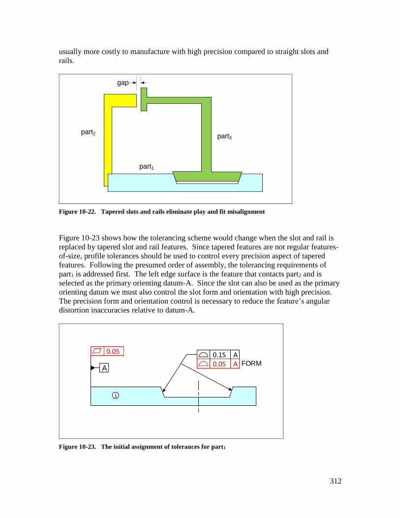
312

usually more costly to manufacture with high precision compared to straight slots and

rails.

part1

part3

part3

part2

gap

Figure 10-22. Tapered slots and rails eliminate play and fit misalignment

Figure 10-23 shows how the tolerancing scheme would change when the slot and rail is

replaced by tapered slot and rail features. Since tapered features are not regular features-

of-size, profile tolerances should be used to control every precision aspect of tapered

features. Following the presumed order of assembly, the tolerancing requirements of

part1 is addressed first. The left edge surface is the feature that contacts part2 and is

selected as the primary orienting datum-A. Since the slot can also be used as the primary

orienting datum we must also control the slot form and orientation with high precision.

The precision form and orientation control is necessary to reduce the feature’s angular

distortion inaccuracies relative to datum-A.

A

0.15 A0.05

0.05 A FORM

1

Figure 10-23. The initial assignment of tolerances for part1

313

The specifications for part2 remain the same as in the previous example while the

specifications for part3 is shown in Figure 10-24.

0.150.05

A

0.15 A

FORM

3


The pair of tapered sliding surfaces is controlled for size using the upper profile statement

to within 0.15 mm. The lower profile statement is for finer control of feature form. This

pair of surfaces is selected as the primary orienting feature. Datum-A defines the center

plane of the tapered slot for controlling horizontal distances.

Example-8: A multipart tolerance design with cylindrical fit features

Consider the simple three-part assembly with cylindrical features as shown in Figure 10-

25. Part numbers indicate the presumed order of assembly.

314

part1

part2

part3

Figure 10-25. A three-part assembly with cylindrical fit features

Figure 10-26 shows the initial theoretical dimensions and tolerances of part1.

Figure 10-26. Initial tolerances for part1

A

B

0.25 A B

0.5 A B

58

50

0.05

0.08 A

0.05 A

1

315

The horizontal surface feature on the right side that contacts part2 is used as the primary

orienting datum. The vertical edge is selected as the secondary locating datum. Since

the left-side vertical surface is an equally valid choice for the primary orienting datum,

the orientation of the vertical surface with respect to datum-A is controlled with high

precision. For part1, the upper features are controlled by profile tolerances.

The theoretical dimensions are selected such that the theoretical axis of the hole and the

theoretical axis of the boss align. This is always the best practice in order to allow the

widest tolerances for fit. Figure 10-27 shows the specifications for part2 and part3.

Ø 0 A BM

Ø 0 A BM

Ø 45.0 – 45.4

75

30

Ø 44.0 – 44.4

88

25

A

B

B A

0.05

0.05

0.08 A

0.08 A

2

3

Figure 10-27. Initial tolerances for part2 and part3

The explanation of these tolerances is left as an exercise.

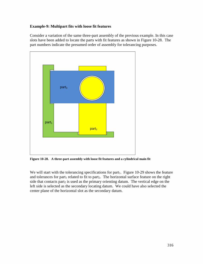
316

Example-9: Multipart fits with loose fit features

Consider a variation of the same three-part assembly of the previous example. In this case

slots have been added to locate the parts with fit features as shown in Figure 10-28. The

part numbers indicate the presumed order of assembly for tolerancing purposes.

part1

part2

part3

Figure 10-28. A three-part assembly with loose fit features and a cylindrical main fit

We will start with the tolerancing specifications for part1. Figure 10-29 shows the feature

and tolerances for part1 related to fit to part2. The horizontal surface feature on the right

side that contacts part2 is used as the primary orienting datum. The vertical edge on the

left side is selected as the secondary locating datum. We could have also selected the

center plane of the horizontal slot as the secondary datum.

317

50.0 – 50.2

0 AM

A

B

0.1 A BL

0.05

0.08 A

1

Figure 10-29. Initial tolerances for the lower slot of part1

The perpendicularity statement for the lower slot is necessary to assure its fit to the rail of

part2 while the lower position tolerance is to control the influence of the size and the

position of the slot on the main fit gap.

We now add the necessary tolerances to the upper slot for the fit of part3. To focus on the

upper slot, the tolerances associated with the lower features are not shown. Figure 10-30

shows the result.

A

60.0 – 60.2

75

88

0 BM

B

0.1 A BL

0.08 A

1

Figure 10-30. Initial tolerances for the upper slot of part1

318

The perpendicularity tolerance is needed because the upper slot has an orientation-

constrained fit to part3. The position tolerance limits the influence of the upper slot on

the fit gap. Figure 10-31 shows the tolerancing of part2 and part3.

M

Ø 45.0 – 45.4

75

59.6 – 59.8

Ø 44.0 – 44.4

88

49.6 - 49.8

25

A

A

0 AM

B

0 AM

B

0 A B L

M0 LA B

0.05

0.05

2

3


Datum-B for both parts is specified at LMB as the fit arrangement of these datum

features is assumed to be unpredictable during assembly. The theoretical positions are

specified such that the center of the hole and boss align.

Example-10: A multipart fit with multiple loose fits

Consider the four-part assembly shown in Figure 10-32. The part numbers indicate the

presumed order of assembly for tolerancing purposes. There are three fit features in the

path of the final fit between the boss and the hole. If the parts are to be put together

randomly, the worst situation for fit is when all slots and rails are at their LMC limit of

size creating the widest slacks in the fits.

319

part2

part1

part3

part4

Figure 10-32. A five-part assembly with three fit features in the path of the main cylindrical fit

Figure 10-33 shows the tolerances for part1.

50.0 – 50.20 AM

A

B

15.0 – 15.10 CM

CL L0.1 A B

0.05

0.05

0.1 A0.05 A

1


The first fit is the slot feature fit to the rail of part2. The perpendicularity tolerance at

MMC is necessary for this orientation-constrained fit. Datum-A is chosen as the primary

320

orienting datum. Datum-C can also be chosen as the primary orienting datum. Datum-A

is selected based on the presumed order of assembly. Since datum-C controls the

orientation of part3, the orientation of datum-C with respect to datum-A is controlled with

high precision to reduce the distortion effects. The slot center plane is chosen as the

secondary locating datum. The rail has a perpendicularity tolerance at MMC for its direct

orientation-constrained fit to the slot of part3.

The position of the rail with respect to the slot is controlled at LMC, assuming this fit

cannot be favorably positioned during assembly. The datum-B is specified at LMB also

because the slot datum feature is a loose fit feature with an unpredictable arrangement

during assembly. Figure 10-34 shows the tolerancing for part3.

45.0 - 45.2

0 AMA

B

15.1 – 15.2

0 CM

C 0.1 AL

A B L0.3

0.05

0.05

0.05 A

3


Datum-A and datum-B are selected as the primary orientating and secondary locating

features. Datum-B slot has an orientation-constrained fit to part1. Datum-C surface

controls the orientation of part4 and for that reason the perpendicularity of datum-C with

respect to datum-A is controlled with high precision. The upper slot has an orientation-

321

constrained fit to part4 resulting in a perpendicularity tolerance specification with zero

value at MMC. The position of the upper slot controls the vertical location of part4. The

slot is controlled with a position tolerance value of 0.1 mm at LMC. Datum-C controls

the horizontal location of part4. A profile tolerance with a value on 0.3 mm is applied to

datum-C surface. This profile tolerance is located with respect to datum-B and since the

datum fit arrangement is unpredictable, the datum-B specification is specified at LMB.

Tolerancing of part2 and part4 are identical to the ones in the previous example.

Example-11: Another multipart fit with multiple loose fits

In the assembly shown in Figure 10-35, part4 is known to be assembled last. The fit

arrangement involving the slot features is unlikely to be adjustable for favorable

positioning during assembly.

part1

part3

part2

part4

Figure 10-35. A four-part assembly

Figure 10-36 shows the features and tolerances of part1. The top surface is the primary

orienting datum. The perpendicularity tolerances are necessary for direct fits and the

position statement is needed to limit the influence of the size and distance between the

slots on the fit of part4 bar. Therefore, the positions of the slot and rail features are

modified by l modifiers.

322

2X 12.1 – 12.2

A

0 AM

A0.3 L 0.05

INDIVIDUALLY

80

1

Figure 10-36. Initial tolerances of part1

Figure 10-37 shows the features and tolerances of part2 and part3. The perpendicularity

tolerance is needed for the direct fit. The position tolerance is necessary to assure the fit

of the final piece, which is the part4 bar. The position tolerance of the cylindrical fit

feature is specified at MMC as this feature fits to the last part and is also the main fit

feature. Since the final arrangement of the slot datum cannot be altered during assembly

the slot datum is specified with an LMB specification.

A

0 AM

M L0.3 A B

12.0 – 12.1B

9.0 – 9.1

0.05

2

3


323

Figure 10-38 shows the features and tolerances of part4 that is placed last into the

assembly.

2X Ø 9.5 – 9.6

Ø 0 M

4


Example-12: Influence of orientation accuracy on fit

When analyzing an assembly for fit we must be aware of orientation deviations that

influence the fit. An example is shown in Figure 10-39.

part1

part2

part3

part4

Figure 10-39. The parallelness of top and bottom surfaces of part1 is critical to fit

The top and bottom plates have forced firm contacts with the two faces of part1 due to the

presence of the fasteners. Sufficient parallelness control should be applied between these

324

surfaces to reduce the distortion effects. Figure 10-40 shows an exaggerated graphic of

this situation.

1

2

3

4

Figure 10-40. The adverse effect of excessive angular distortion on fit

Consider the specifications shown in Figure 10-41 for part1. The top and bottom surfaces

must be sufficiently parallel to reduce the projection distortion effect. The parallelness

tolerance statement is shown in green. The explanation of tolerances for part2 and part4 is

straightforward and left as an exercise. The perpendicularity tolerance is necessary to set

up a reference surface (datum) for locating the fastener holes. Neither the datum label

not the fastener holes are shown. The profile tolerance controls the height of the block for

proper fit to the end part (part4). The explanation of tolerances for other parts is left as an

exercise.

325

29 +/- 0.5

A

A

0 A

A

0.1 A

0.02

0.05

0.05

M

1

4

3

0.03 A

0.25 A

0.05 A

Figure 10-41. Initial assignment of tolerances

Figure 10-42 shows the maximum possible deviation caused by the angular projection

effect when only the size tolerance (t = 1 mm) is specified without parallelness control.

t

L

d

H

Figure 10-42. The magnified effect of distortion error when projected out a long distance

326

The size tolerance of the block is t = 1 mm, the length of the overhang, or projection, is

L=50 mm, the width of the block is H=10 mm, and is the vector that represents the

effect of angular distortion. can be found as

mmtH

L5d

This vector is similar to the parallelness tolerance except that its value is magnified by

the projection length. The vector is shown pointing downward but it can point in either

direction.

Example-13: A multipart assembly with a press fit insert

In the assembly shown in Figure 10-43, part1 is attached to the frame of a machine. The

location of part1 on the machine is not important. Part1 has a boss which fits the inner

diameter of a plain bearing or bushing (part4). The bushing is press-fit into the bearing

hole in part3. Part3 with the part4 insert is placed last into the assembly.

Machine Frame

part3,4

part2

part1

Figure 10-43. A multipart assembly with a press-fit bearing

The assembly requires the parts to be put together according to the order indicated. The

final arrangement of the slot and rail fit between part1 and part2 is unpredictable during

assembly. Figure 10-44 shows the tolerance specifications for part1. The basic

dimensions are selected such that the theoretical axis of the hole and the theoretical axis

of the boss align.

327

18.0 – 18.1

Ø 25.1 – 25.3

88

100

A

B

Ø 0 AM

2 SURFACES

0.05

LM0 A B

1

Figure 10-44. Initial tolerance assignment for part1

Datum-A is the primary orienting surface. The flatness tolerance controls the flatness

and co-planarity of the datum-A pair of surfaces. The rail perpendicularity tolerance is

for the orientation-constrained fit to the rail of part2. Since the fit of the rail is

unpredictable during assembly the l modifier will be used when referenced as a datum

such as in the position tolerance statement. Figure 10-45 shows the initial basic

dimensions and tolerances for part2.

328

18.4 – 18.6

86.0 – 86.2

100

40

A

Ø 0.08

2 SURFACES

Ø 0 AM

B

0.12 ALM0.2 A B

Ø 0 CM

C

0.05 A

2


The primary orienting surfaces are chosen as datum-A. The slot is selected as the

secondary locating datum-B. The surface designated as datum-C orients part3,4 and is

specified to be parallel to datum-A with high precision. The slot and rail features are set

up for orientation-constrained fits. Since the slot fit is in the path of main fit and its fit

arrangement is unpredictable, the slot datum is referenced LMB with an l modifier.

The fit of the rail itself, however, is predictable as it fits last. For that reason, the rail

feature is used with an m modifier. Figure 10-46 shows the initial basic dimensions and

tolerances for part3 and the insert part4. The tolerances involving press-fit inserts were

presented before in Chapter-9.

329

86.4 – 86.6

Ø 30H7

Ø 30k7

Ø 25H7

48 A

Ø 0 AMB

A

Ø 0.05 A

0.05

M0.1 A B

3

4


The 30H7/k7 creates a tight fit between the insert and the hole. For this last part to be

inserted into the assembly the slack in the slot and rail fit can be adjusted during

assembly to achieve a fit, hence, the slot datum reference is modified at MMB.

Example-14: Design for function - cutting blades

Figure 10-47 is a simple representation of a pair of cutter blades firmly attached to a

spindle. The attachment screws are not shown. It is important to control the distance

between the ends of the blades. It is also important for the blades to be prependicular to

the axis of the spindle to prevent axial wobble and vibration of the cutting blades. The

most important aspect of the function of the assembly is for the distance between the two

blades to remain constant with high precision. A constant distance between the blades

creates cleaner cuts and reduces vibration and cutting forces.

330

Figure 10-47. A schematic representation of a pair of cutting blades

Figure 10-48 shows the required tolerances for the spindle. The function related

specifications are shown in blue.

20h620h6

15h8

AB

0.05 A-B

C

0.01

0.02 C

0.05 A

BOTH SIDES

Figure 10-48. Initial tolerances for the spindle

The high precision parallelness assures a constant distance between the two blades. The

runout tolerances keep the surfaces square to the axis of rotation.

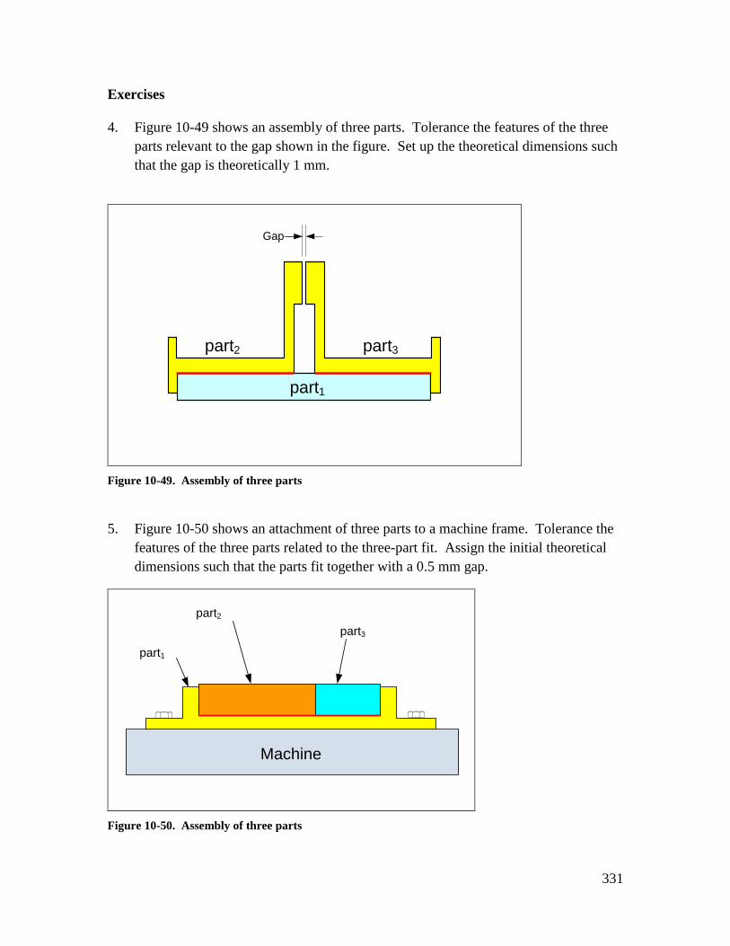
331

Exercises

4. Figure 10-49 shows an assembly of three parts. Tolerance the features of the three

parts relevant to the gap shown in the figure. Set up the theoretical dimensions such

that the gap is theoretically 1 mm.

part1

part2 part3

Gap

Figure 10-49. Assembly of three parts

5. Figure 10-50 shows an attachment of three parts to a machine frame. Tolerance the

features of the three parts related to the three-part fit. Assign the initial theoretical

dimensions such that the parts fit together with a 0.5 mm gap.

part2

part1

part3

Machine

Figure 10-50. Assembly of three parts

332

6. Figure 10-51 shows an attachment of three parts to a machine frame with loose bolts

and nuts. Tolerance the features of the three parts related to the three-part fit. The

bolts and nuts are M8. The dimensioning of one the T-shaped part is shown in

Figure 10-52.

Figure 10-51. Assembly of three parts with loose bolts and nuts

Figure 10-52. Dimensions of the T-shaped part

333

7. Figure 10-53 shows an attachment of four parts to a machine frame. Tolerance the

features of the parts relevant to this four-part fit. Assume part2 and part3 are

identical and are glued to part1. Part4 is always the last part to be assembled. Set up

the theoretical dimensions such that the fit gap between part4 and part2 is 1 mm.

part-2

part-1

part-3

Machine

part-4

Figure 10-53. Assembly of four parts

8. Figure 10-54 shows a three-part assembly. Specify the tolerances necessary to allow

a fit between the three parts. Part2 and part3 are identical and must have identical

specifications. It is not necessary to show the tolerances related to two-part fastener

fits.

334

part1

part3part2

Figure 10-54. Three-part assembly

9. Figure 10-55 shows a bearing assembly. Model the assembly and the two parts of

the housing using your CAD system and add all the dimensions and tolerances

necessary for the proper fit of the parts. Use tolerance values consistent with the

machining processes. There is no need to model the bearings or the shaft. Figure 10-

56 shows the drawing of the base part with its dimensions.

Figure 10-55. Bearing assembly

335

Figure 10-56. Drawing of the lower part of the housing

10. Figure 10-57 shows a hand crank assembly. Model the bottom plate and one of the

two side plates using your CAD system and add the dimensions and tolerances

necessary for the proper fit of the parts. Use tolerance values consistent with the

machining processes. There is no need to model the bearings or the shaft.

336

Figure 10-57. The hand crank assembly

Figure 10-58 shows the drawing of the bottom plate with its overall dimensions. The rest

of the dimensions are up to you.

337

Figure 10-58. The bottom plate of the hand crank assembly

338

Chapter 11 Tolerance Analysis of Multipart Fits

11.1. Overview

This chapter introduces tolerance analysis methods for calculating fit clearances in

multipart fits. Multipart tolerance analysis can be done graphically with the aid of a CAD

system or analytically. In the graphical method, the designer models the parts in a CAD

system, puts them together into an assembly, and checks the fit gap. The graphical

tolerance analysis method is intuitive and helpful in developing a feel for how changes in

dimensions and tolerances influence the fit gap. After becoming more experienced with

the graphical analysis method, you can use the quicker analytical method in which the

gap value is written as a function of the given dimensions and tolerances. The analytical

tolerance method allows a designer to quickly evaluate the consequences of changing the

theoretical dimensions or tolerance values on the fit or function of an assembly. The

analytical method can also be automated through computer programming. With an

effective user interface an analysis program allows a designer to obtain quick and error-

free solutions. Such computer programs can also create random simulations of part

geometries and allow statistical evaluation of design dimensions and tolerances. The

program TAP (Tolerance Analysis Program), which can be downloaded from the book

web site, is an example of such a program. To illustrate tolerance analysis methods we

will analyze some of the same example assemblies for which the tolerance design task

was completed in Chapter-10.

11.2. Tolerance analysis overview

Tolerance analysis starts with the selection of a critical assembly dimension whose value

depends on the theoretical dimensions and tolerances of other features and other parts.

The designer sets acceptable limits for the selected assembly dimension and finds a

combination of theoretical dimensions and tolerance values that would meet the selected

assembly dimension targets. Most of the problems in tolerancing deal with fit application

for which the critical dimension is a gap. The minimum value of the gap is usually set to

zero for fit purposes and the resulting maximum value is accepted and left unspecified.

The reason a check on maximum gap is usually unnecessary is that when care is

exercised to ensure a minimum gap of zero, the maximum gap value becomes just an

accumulation of the tolerance values. Usually, an accumulation of a few tolerances does

not add up to objectionable values in constrained fits. Sometimes, however, the

maximum gap must be controlled with precision for other functional reasons. When the

initial tolerance values do not meet the maximum gap requirements, one or more of the

following four options can be explored:

1. The design can be changed such that the critical gap is influenced by fewer

tolerance values.

2. The design can be changed such that adjustments and alignments can be made

during assembly for some fits. For example a design may allow shims to be used

339

to adjust distances. Assembly time adjustments reduce the need for high

precision features.

3. A degree of risk can be accepted regarding the gap exceeding the acceptable

limits in rare cases.

4. Tolerance values can be reduced.

The first step in tolerance analysis is to determine the dimensions and tolerances that

influence the fit gap. In the analytical method, each dimension and each tolerance will be

represented by a vector. The size of each vector will correspond to a basic dimension

value or a combined dimension and tolerance value. These vectors, along with the gap

vector, form a loop called the tolerance loop. The proper identification of the tolerance

loop vectors is the most important step in the fit analysis as the rest of the work is

mathematical and can be left to a computer program. Tolerance analysis will be

illustrated in the context of a variety of problems using both graphical and analytical

methods.

11.3. Examples

Example-1: A simple tolerance design problem: The assembly for Example-1 in

Chapter-10 is shown in Figure 11-1. We like to select the theoretical dimensions and

tolerance values for a minimum gap of zero.

part1

part2

part3

Figure 11-1. An example of a fit involving two dimension values

Figure 11-2 shows the initial selection of theoretical dimensions and tolerance values.

While any initial theoretical dimension or tolerance value can be selected, reasonably

close values to the final solution are preferred as they provide a degree of error checking.

340

A A

0.1 A

50

0.1 A

51

0.05 0.05

23

Figure 11-2. Profile tolerances control the fit gap

Graphical Method

In a CAD system, we can quickly create simple sketches that incorporate the important

dimensions and tolerances necessary to find a minimum or maximum gap. The better

graphical method approach is to create the 3D solid models of parts and bring them into

an assembly. For simple analysis problems, however, we can use the quicker sketch

assemblies. Figure 11-3 shows a simple sketch assembly model for this problem. Note

that we only need to draw the lines necessary to capture the needed dimensions. The

final sketch need not look like the actual design.

Figure 11-3. CAD sketch model of the assembly

341

Within the scope of allowed tolerances, the two important dimensions are set to values

that lead to the minimum gap. Including the profile tolerances, the smallest dimension on

part2 is 50.95 mm while the largest dimension on part3 is 50.05 mm. Since the resulting

minimum gap is 0.9 mm, we need to change the theoretical value of one of the

dimensions by 0.9 mm. For example, we can reduce the 51 mm dimension in part2 to

50.1 mm. We should then check the gap to make sure it is set to zero as it is not always

easy to know the direction in which a dimension influences the gap.

Figure 11-4 shows the 3D solid model of the assembly using the given design

dimensions. The 0.90 mm distance is the gap value between the two surfaces.

Figure 11-4. 3D model of the assembly

When sketch assemblies become too crowded or confusing the 3D modeling is the best

way to avoid errors.

342

Analytical Method

Figure 11-5 shows the vectors that influence the gap and form a tolerance loop. Vectors

Aa and Ba are associated with profile tolerances on single parts and represent the actual

distances of the controlled surfaces with respect to their datum planes.

G

Ba

Aa

Figure 11-5. Vectors represent variable dimensions controlled by tolerances

We can write an expression for the tolerance loop and the gap vector as

G + Aa – Ba = 0 G = Ba – Aa

The minimum gap expression is

Gmin = (Ba)min – (Aa)max

The value of an actual vector in the tolerance loop can be represented as the sum of a

theoretical dimension vector and a deviation vector. In this case, the deviation vector is

associated with a profile tolerance

Aa = A + dA

And

Ba = B + dB

Where A and B are the theoretical dimensions and dA and dB are the deviation vectors.

The deviation vectors can be positive or negative. The gap vector can be written as

G = (B + dB) - (A + dA)

The minimum value of the gap occurs when the deviation vectors assume their largest

values. The largest value of the deviation vector is given by half of the profile tolerance

value. The minimum gap expression becomes

Gmin = (B - ½ TB ) – (A + ½ TA)

Separating the dimensions and tolerances

Gmin = (B - A) – (½ TA + ½ TB)

The solution procedure in tolerance analysis calls for the initial selection of all tolerance

values based on processes believed to have sufficient accuracy for the application. This

selection is done during the tolerance design step. In this case, the following tolerance

values are selected as shown on the design drawing:

343

TA = TB = 0.1 mm

The tolerance terms add up to

T = (½ TA + ½ TB) = ½ (0.1 + 0.1) = 0.1 mm

The initial value of theoretical dimensions term in the loop equation is

D = (B - A) = 51 – 50 = 1 mm

Therefore

Gmin = D - T = 1 – 0.1 = 0.9 mm

As expected the minimum gap for the initial design is 0.9 mm. We like to adjust one of

the initial basic dimensions to set the minimum gap to zero. Unless other factors favor a

particular selection, the choice of which dimension to adjust is arbitrary. In this case A is

accepted with its initial design value of A = 50 and B can be determined from the Gmin

equation

D = Gmin + T

Resulting in

B – 50 = 0 + 0.1 B = 50.1 mm

The selected theoretical dimensions and tolerances now assure a minimum gap of zero.

The result agrees with the graphical solution method. Although usually unnecessary, we

can check to see how well these choices do on the maximum gap. In this case:

Gmax = (B - A) + ½ (TA + TB)

Note that when Gmin is zero:

(B - A) = ½ (TA + TB)

The maximum gap expression becomes

Gmax = (TA + TB)

Substituting the numbers results in

Gmax = (0.1 + 0.1)

Or,

Gmax = 0.2 mm

Table 11-1 shows the minimum and maximum dimension values associated with profile

vectors when the profile tolerance is equally distributed about the theoretical profile.

When using the graphical method for minimum or maximum gap check, these values

should be used in the modeling of the dimensions.

Vector in gap

function

Tolerance

Type

Tolerance

Value

Minimum

value

Maximum

value

Aa Profile T A – ½ T A + ½ T

Table-11-1. Dimension limits for vectors associated with a profile tolerance

Comparing the graphical and the analytical methods we see that in the graphical method

the tolerance loop is created implicitly through a geometric construction. In addition, the

CAD system performs the additions and subtractions necessary to set the minimum gap

to zero to calculate the unknown dimension.

The computer automated version of the analytical method provides a quick and error-free

way of tolerance analysis. The procedure involves developing the gap expression and

344

entering the data for the vector components in the gap expression. For this program the

gap expression is

G = Ba – Aa

Figure 11-6 shows the input and output dialog window of the program. The left-side

array of rows is where the user inputs the vector information. This program allows

analysis of tolerance loops with up to 10 vectors.

Figure 11-6. The tolerance analysis program dialog screen for Example-1

In this problem, there are two vectors both associated with profile tolerances. The first

vector shown in the first row, Ba, has a +1 coefficient in the gap formula and its initial

design specification has a minimum value of 50.95 mm and a maximum value of 51.05

mm. The second vector, Aa, has a -1 coefficient in the gap formula and has a minimum

value of 49.95 mm and a maximum value of 50.05 mm. The data that defines this gap

model can be saved in a worksheet, in this case it is saved in Example-1 worksheet.

Once saved, a model can be loaded for further analysis at a later time. The right-hand

side of the dialog window shows the analysis results. The top part indicates the worst-

case minimum and maximum gaps. In this case the minimum gap is 0.9 mm. To reset

the minimum gap to zero we can reduce Ba limits by 0.9 mm to a new range of 50.05 mm

to 50.15 mm.

The statistical analysis frame shows the results of twenty thousand random simulations

every time the calculate command button is pushed. In each simulation a random value

between 50.95 and 51.05 is selected for Ba variable and a random value between 49.95

and 50.05 is selected for the Aa variable. All random selections are based on uniform

distributions in which any number between the limits is equally likely to be generated.

In this case the results show that 99.9% of all the assembly gaps are larger than 0.905 mm

and 99.9% of all assembly gaps are smaller than 1.096 mm.

345

Example-2: A simple four-part tolerance analysis problem: The assembly and

tolerancing scheme for Example-2 in Chapter-10 is shown in Figures 11-7, 11-8, 11-9,

11-10, and 11-11. We like to select the theoretical dimensions and tolerance values for a

minimum gap of zero. In this problem, all fit related dimensions are controlled by profile

tolerances except one dimension in part2 which is controlled by a size tolerance.

Gap

part1

part2

part3part4

Figure 11-7. An example of a fit involving four parts

A

50.1 A 0.05

0.06 A


346

5.0 – 5.1

0 M

0.05A

0.06 A


A

0.1 A

51

0.05

3


347

A

0.1 A

50

0.05

4

Figure 11-11. Tolerancing of part4 in the example assembly.

Graphical Method

The tolerance loop for this problem is shown in Figures 11-12. Vector G represents the

gap of interest and other vectors represent the actual dimensions a feature can take given

their tolerances. The tolerance loop shows the dimensions that need to be modeled for

the fit analysis.

G

Aa

Fa

Ca

Da

1 2

3 4

Figure 11-12. Tolerance loop showing the dimensions influencing the gap.

348

Creating a table of dimension values that leads to the minimum gap helps with the

organization of the process. By visualizing how the gap changes when one vector size is

changed, we can determine which dimension limit leads to the minimum gap. The

following table shows the necessary modeling dimensions and their values for the

minimum gap.

Dimension Part Initial Values State

(Ca)min Part1 4.95 -

(Da)min Part3 50.95 -

(Aa)max Part4 50.05 -

(Fa)max Part2 5.1 MMC

Figure 11-13 shows that the minimum gap based on the initial design dimensions and

tolerances is 0.75 mm.


If we choose to adjust the 50.95 mm dimension on part3 to achieve the zero minimum

gap, we need to reduce that value to 50.2 mm. The theoretical 51 mm is subsequently

reduced by 0.75 mm to 50.25 mm. To check, we can enter the new 50.2 mm value in the

model and evaluate the minimum gap, which should become zero. We can enter the new

value in the dimension table to have a record of the new design dimensions as shown in

the following table. The shading indicates the value that is altered in order to achieve the

zero gap value.

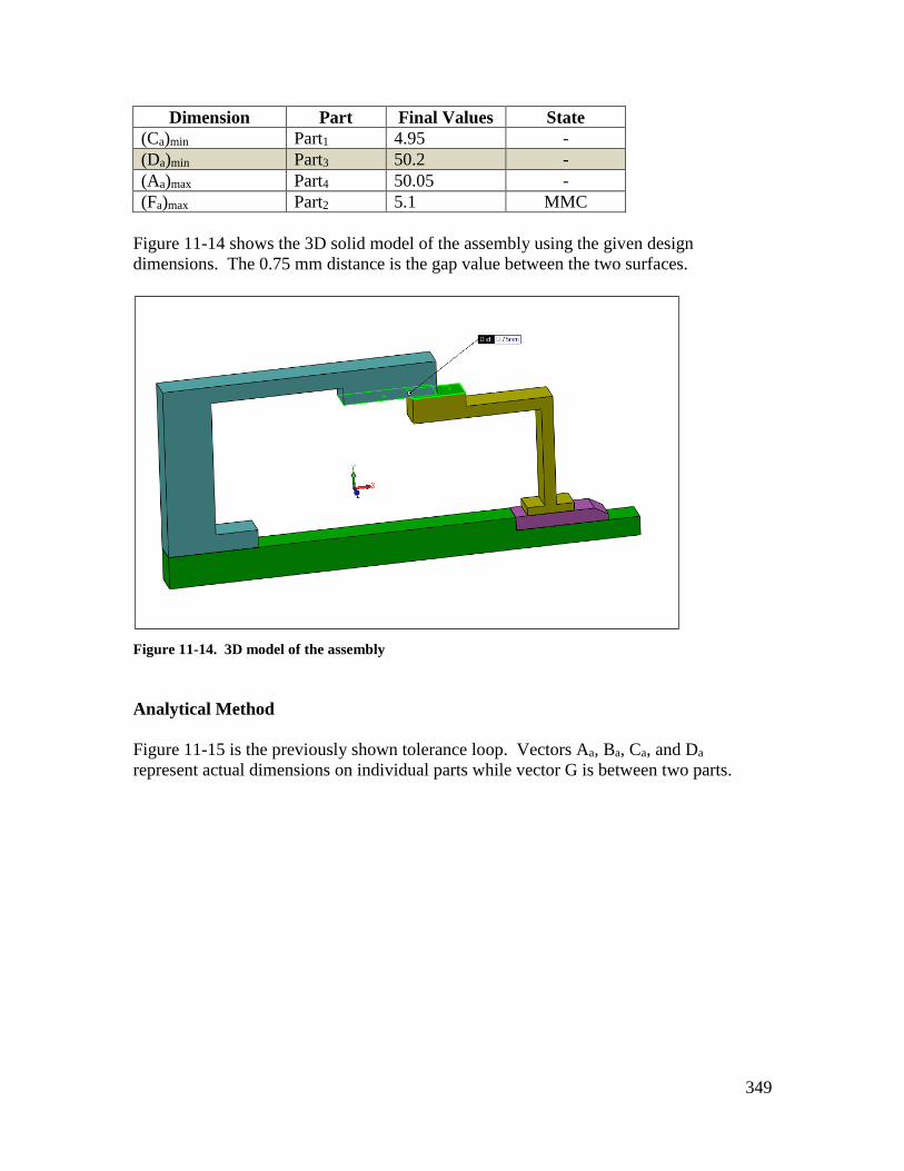
349

Dimension Part Final Values State


(Da)min Part3 50.2 -


(Fa)max Part2 5.1 MMC


dimensions. The 0.75 mm distance is the gap value between the two surfaces.


Analytical Method

Figure 11-15 is the previously shown tolerance loop. Vectors Aa, Ba, Ca, and Da

represent actual dimensions on individual parts while vector G is between two parts.

350

G

Aa

Fa

Ca

Da

1 2

3 4

Figure 11-15. Tolerance loop for tolerance analysis

Vectors Aa, Ca, and Da are associated with profile tolerances while Fa is a size dimension.


Gmin = (Ca)min + (Da)min - (Aa)max - (Fa)max

We can express Fa vector as an actual cross-sectional size vector plus a form deviation

vector

Fa = Fac + dT

Where Fac is the actual cross-section size and dT is a deviation vector due to the geometric

tolerance, in this case flatness. The cross-sectional size limits are the specified LMC and

MMC limits, or Fmin and Fmax. The minimum and maximum values for the Fa vector,

when the tolerance is m modified are

(Fa)min = Fmin

(Fa)max = Fmax + TF

The minimum value of the gap including the geometric tolerances is

Gmin = (C + D - A) - Fmax - ½ (TC + TD + TA)

We can now set the following values based on the initial design

A=50

B = C = 5

TA = TC = TD = 0.1 mm

Setting Gmin = 0 and solving for D results in

D = Gmin + (A - C) + (Fmax + TF) + ½ (TA + TC + TD)

Substituting the values

D = 0 + (50 -5) + (5.1 + 0) + ½ (0.1 + 0.1 + 0.1) D = 50.25 mm

The solution agrees with the graphical solution. We can also check the resulting

maximum gap as

Gmax = (Ca)max + (Da)max – (Aa)min – (Fa)min

In calculating the maximum gap, the feature-of-size is assumed to be in its LMC state.

Including the tolerances, the maximum gap is

Gmax = (C + D - A) – Fmin + ½ (TA + TC + TD)

Substituting the numbers

351

Gmax = (5 + 50.25 – 50) – 5 + ½ (0.1 + 0.1 +0.1)

Gmax = 0.4 mm

If this value of Gmax is unacceptable, one or more of the remedies mentioned earlier in

this chapter’s introduction should be explored.

Figure 11-16 shows the input and output information of the TAP program for this

example using the initial design values. The first row is for vector Ca, the second row is

for Da, the third row is for Aa, and the fourth row is for Fa.

Figure 11-16. The tolerance analysis program dialog screen for Example-2 with initial values

To reset the gap to zero we can reduce the second vector limits by 0.75 mm to a range of

50.2 mm to 50.3 mm. The result is shown in Figure 11-17.

352

Figure 11-17. The tolerance analysis program dialog screen for Example-2 with final values

Example-3: A simple four-part fit with features-of-size

The assembly and tolerancing scheme for Example-3 in Chapter-10 is shown in Figure

11-18 and 11-19. We like to specify the theoretical dimensions and tolerance values for a

minimum gap of zero.

part1

part2 part3

part4

Figure 11-18. A four-part assembly with two fit features

353

A

100 – 100.1

Ø 0 AM

A

A

B

5

0.1 A B

100.1 – 100.2

Ø 0 AM

0.05

0.05

0.05

0.08 A

A

0.05 A

2

4

1


Graphical Method

To prepare for the graphical analysis or the analytical analysis, we identify the tolerance

loop vectors as shown in Figure 11-20.

G

AaBa

F2a

F1a

1

2

3

4


354

The following table indicates the initial dimension limits used in the graphical modeling

of the parts that lead to the minimum gap. For example, if we visualize increasing the F2a

dimension in the figure, the gap will increase. Therefore, we set the F2a dimension to its

minimum value. The table also indicates the final value that leads to a zero minimum

gap in parenthesis.

Dimension Part Initial Value (Final Value) State

(F2a)min Part1 110.1 (100.2) LMC

(F1a)max Part4 100.1 MMC


(Ba)max Part2 5.05 -

Figure 11-21 shows the sketch assembly with dimensions as specified in the initial design

along with tolerances that lead to the minimum gap. The initial design leads to an

interference of 0.1 mm.

Figure 11-21. CAD sketch model of the assembly for minimum gap

To set the minimum gap to zero, we need to adjust one of the theoretical dimensions. In

this case, we can increase the width limits of part1 by 0.1 mm to a range of 110.2 – 110.3

mm.

355

To find the resulting maximum gap we have to set the dimensions and tolerances to

values that lead to the maximum gap. The following table indicates the dimension limits

to be used in the graphical modeling of the parts that lead to the maximum gap.

Dimension Part Modeling Values State


(F1a)min Part4 100.0 LMC

(Aa)min Part3 4.95 -

(Ba)min Part2 4.95 -

Figure 11-22 shows the sketch assembly with the dimension values that lead to the

maximum gap.

Figure 11-22. CAD sketch model of the assembly for maximum gap

In this case the maximum gap that can result from the specifications is 0.4 mm. Figure

11-23 shows the 3D solid model of the assembly using the initial design dimensions that

leads to an interference of 0.1 mm.

356


Analytical Method

To perform the tolerance analysis, we identify the tolerance loop vectors as shown in

Figure 11-24.

G

AaBa

F2a

F1a

1

23

4


357

The loop equation is

G + F1a + Aa - F2a + Ba = 0 G = F2a - F1a – Aa – Ba


Gmin = (F2a)min – (F1a)max – (Aa)max – (Ba)max

Aa and Ba vectors are associated with profile tolerances. F1a and F2a are size vectors

associated with orientation tolerances. Including the tolerance vectors, the minimum

assembly gap can be expressed as

Gmin = F2min – (F1max + TF1) – (A + ½ TA) – (B + ½ TB)

Separating tolerance terms

Gmin = (F2min – F1max – A – B) - (½ TB + TF1 + ½ TA)

Initial size tolerances and orientation tolerances are assigned based on the intended

processes. In this case we select the following size tolerances

tF1 = tF2 = 0.1

Since zero perpendicularity tolerances are used

TF1 = TF2 = 0

The profile tolerances are selected to be

TA = TB = 0.1

The following three dimensions are set based on initial design specifications

A = B = 5 F1max = 100.1

Substituting into Gmin = 0 we find F2min = 110.2 mm. Since the size tolerances are 0.1

mm, we can find F2max = 110.3 mm. The new size limits for the rail features are

F1min =100.0 F1max=100.1

F2min =110.2 F2max =110.3

This result agrees with the graphical method. We can now check the maximum gap. The

Gmax expression is

Gmax = F2max – F1min – (A - ½ TA) – (B - ½ TB)

Substituting values for dimensions and tolerances, we get:

Gmax = 110.3 – 100 – (5 - ½ (0.1)) – (5 - ½ (0.1))

Gmax = 0.4 mm

When a size vector is associated with a form or orientation tolerance, the form or

orientation deviation vector can be combined with the size vector into a fit-equivalent

size. Table 11-2 shows the minimum and maximum values of the combined size and

geometric deviation vector. These relationships are also used in the graphical modeling

for fit-equivalent sizes.

Vector

in Gap

Function

Tolerance

Type

Specified

Tolerance

Minimum Value Maximum Value

Fa (Pin) Form or

Orientation TF @ m Fmin Fmax + TF

TF Fmin Fmax + TF

TF @ l Fmin Fmax + TF + tsF

Ha

(Hole) TH @ m Hmin – TH Hmax

TH Hmin – TH Hmax

TH @ l Hmin - TH - tsH Hmax

Table-11-2. Dimension limits for vectors associated with a form or orientation tolerances

358

For example, if a 20-21 mm pin feature has a perpendicularity tolerance of 0.5m, the

specification corresponds to the first row of the table. The minimum value of the

combined size and geometric deviation vector for this feature would be its LMC size of

20 mm. The pin’s largest combination of size and perpendicularity deviation vector

would be the sum of the pin’s MMC size and its perpendicularity at MMC, which

becomes 21.5 mm.

Figure 11-25 shows the TAP results for the final dimensions that lead to a zero minimum

gap.


Example-4: Retaining ring fit on a gearbox shaft

The assembly and tolerancing scheme for Example-4 in Chapter-10 is shown in Figure

11-26. We like to specify the theoretical dimensions and tolerance values for a minimum

gap of zero. The maximum gap must not exceed 0.25 mm in order to limit the axial play

of the gear.

359

Figure 11-26. A gearbox shaft with a retaining ring fixing the axial location of the gear

The initial dimensions and tolerances that control the gap are shown in Figure 11-27.

B

30 +/- 0.05

1 +/- 0.02

31.5

1.04-1.14

0.05

Purchased Parts

A

0.05 A B


360

Graphical Method

The gap of interest is the distance between the gear face and the retaining ring face. A

tolerance loop can be developed incorporating all the relevant features influencing this

gap. Figure 11-28 shows the tolerance loop. The G vector represents the play in the fit.

Aa

F2aF1a

G

1

2

3

Figure 11-28. The tolerance loop

The following table indicates the initial dimension limits used in the graphical modeling

of the parts that lead to the minimum gap. The table also shows the final value of one

dimension that leads to a zero minimum gap. The width of the gear is set to its maximum

30.05 mm value and the thickness of the ring is also set to its maximum value of 1.02

mm. The other relevant dimension is the distance associated with the right edge of the

groove which is controlled by a profile tolerance. A dimension value of 31.475 mm is

used as the minimum distance of the right groove edge relative to the shaft shoulder.


(Aa)min Part1 31.475 (31.075) -



Figure 11-29 shows the relevant parts of the sketch assembly with dimensions resulting

in the minimum gap.

361


The initial design results in a minimum gap of 0.405 mm. We need to reduce the

theoretical distance of the right edge of the groove by 0.405 mm in order to set the

minimum gap to zero. This results in (Aa)min = 31.07 mm and theoretical dimension of A

becomes 31.095 mm. We can round up this value to 31.1 mm, allowing a theoretical

minimum gap of 0.005 mm. With this new value of A = 31.1 mm, the maximum gap can

be shown to become 0.195 mm.

Figure 11-30 shows the cutaway of the 3D solid model of the assembly using the initial

design dimensions. The 0.405 mm distance is the gap value between the gear and ring

surfaces.

362


One of the advantages of the graphical solution is that the designer can check for other

problems. In this case the gear width does not go beyond the edge of the groove. This

can be corrected by widening the groove by 0.1 mm from 1.43 mm to 1.53 mm. Figure

11-31 shows that the groove size adjustment solves the problem. The minimum and

maximum gaps are defined by the faces of the ring and the gear.

363

Figure 11-31. 3D model of the assembly after widening the groove size

This problem is an example of a tolerance analysis problem with multiple assembly

variables. In this case both the fit gap and the amount of gear overhang are important. A

solution was easy to find for the problem because increasing the width of the groove does

not affect the gap value. The right edge of the groove controls the gap and that is

controlled directly by the profile tolerance. In other multi-criteria cases, finding a

solution based on graphical approach becomes difficult. In the analytical approach we set

up a second loop equation for the overhang and solve for the dimension limits and

tolerances that satisfies the requirements of both criteria. Multiple criteria problems are

formulated just like single criterion problems. They do, however, lead to multiple

equations that need to be solved simultaneously.

Analytical Method

Using the tolerance loop a minimum gap expression is developed as

Gmin = (Aa)min – (F2a)max – (F1a)max

Setting Gmin = 0 and solving for A results in

0 = (A - 0.025) – 1.02 – 30.05

A = 31.095 mm

This value can be kept as a theoretical dimension or, accepting a minimum gap of 0.005

mm, it can be rounded up to

A = 31.1 mm

The maximum gap expression is

Gmax = (Aa)max – (F2a)min – (F1a)min

364

Substituting the values we get

Gmax = 31.225 – 0.98 – 29.95

Gmax = 0.295 mm

As an exercise, you can set up the loop equation for the overhang and determine the

overhang limits based on A = 31.1 mm solution and groove size limits of 1.43 to 1.53

mm. Is the overhang value positive?

Figure 11-32 shows the TAP results for the final dimensions that lead to a zero minimum

gap.


The statistical results show that 99% of assemblies will have a gap greater than 0.02 mm

and 99% of assemblies will have a gap less than 0.224 mm.

Example-5: Thermal expansion gap of a gearbox shaft

The assembly for Example-5 in Chapter-10 is shown in Figure 11-33. The figure also

shows the tolerance loop. We like to set up the theoretical dimensions and tolerance

values for a minimum gap of 0.25 mm. The maximum gap must not exceed 0.7 mm.

This problem will only be solved using the analytical method.

365

F1a F2a

Ca

G

part1

part2

part3

part4

part5

Ba

F3a

Figure 11-33. The gap dimension in this gearbox depend on six part dimensions


G + F1a + F3a + F2a + Ba – Ca = 0

Gmin expression becomes

Gmin = (Ca)min – (F1a)max – (F2a)max – (F3a)max – (Ba)max

Adding the tolerance vectors

Gmin = (C – ½ TC) – F1max – F2max – F3max – (B + ½ TB) We can solve for B dimension

B = (C – ½ TC) – F1max – F2max – F3max – ½ TB – Gmin

The initial tolerance specifications for custom parts are shown in Figure 11-34. The

standard bearing width size limits are 9.95 – 10.00 mm.

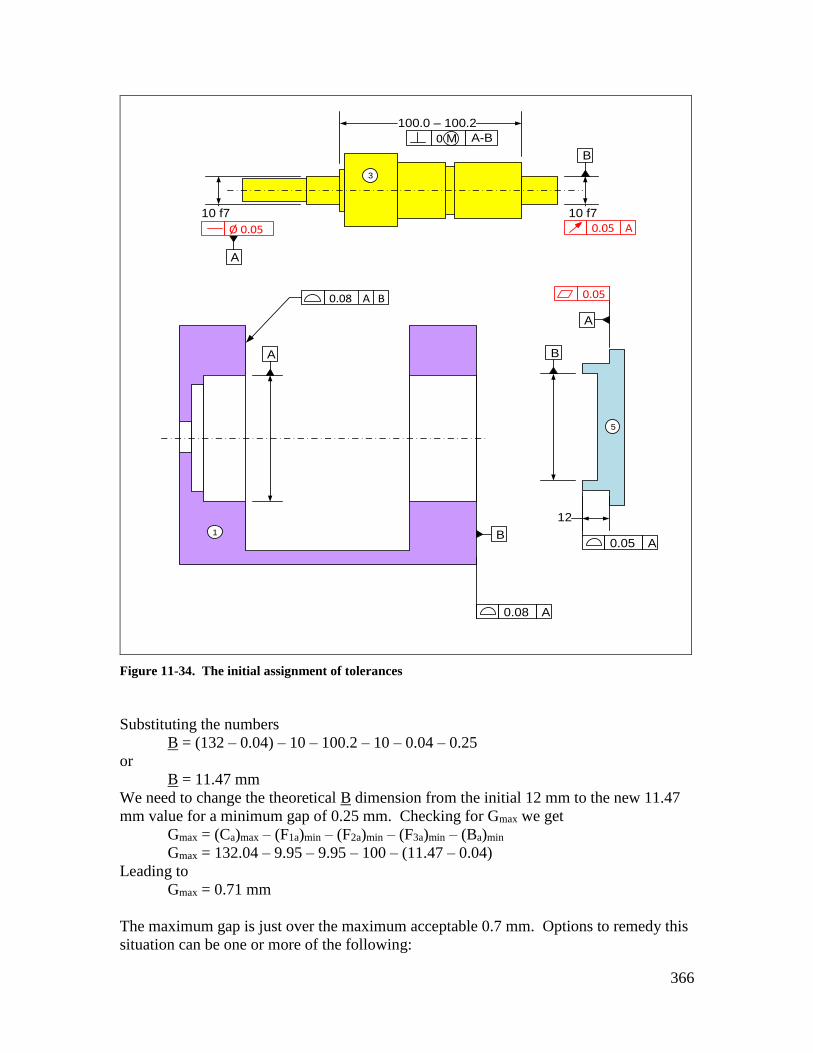
366

100.0 – 100.2

A

A

A

0.05 A

0 AM

0.05

Ø 0.05

10 f7

12

10 f7

B

A-B

0.05 A

B

B

0.08 A B

0.08 A

1

5

3



B = (132 – 0.04) – 10 – 100.2 – 10 – 0.04 – 0.25

or

B = 11.47 mm

We need to change the theoretical B dimension from the initial 12 mm to the new 11.47

mm value for a minimum gap of 0.25 mm. Checking for Gmax we get

Gmax = (Ca)max – (F1a)min – (F2a)min – (F3a)min – (Ba)min

Gmax = 132.04 – 9.95 – 9.95 – 100 – (11.47 – 0.04)

Leading to

Gmax = 0.71 mm

The maximum gap is just over the maximum acceptable 0.7 mm. Options to remedy this

situation can be one or more of the following:

367

Accept the slight risk of the gap exceeding 0.7 mm and accept the solution.

Slightly reduce some size or profile tolerances and solve for new B.

Set up the minimum gap to a value slightly smaller than 0.25 mm.

Figure 11-35 shows the TAP results for the final dimensions that lead to 0.25 mm

minimum gap. Note that if each deviation follows a uniform random distribution pattern

within a range defined by tolerances, 99.9% of all the assemblies would have a maximum

gap of less than 0.6 mm.


Example-6: A multipart tolerance design with loose fit features

The assembly of Example-6 in Chapter-10 and the initial tolerance assignments are

shown in Figure 11-36 and 11-37 and 11-38. In this problem we have a vector that is

associated with a position tolerance. We like to adjust one of the theoretical dimensions

to obtain a zero minimum gap with the given tolerances.

368

part1

part3part2

main gap

Figure 11-36. A multipart assembly with loose fit features

A

20.0 – 20.1

40

B

0 AM

0.3 A BL

0.05

0.08 A

1

Figure 11-37. Tolerances of part1 and the slot feature assuming the final arrangement of the slot fit is

unpredictable during assembly

369

A

19.8-20.0

20

B0 AMA

B

0.1 A BL0.1 A B

0.05

0.050.08 A


Graphical Method

Figure 11-39 shows the tolerance loop for this example. When modeling, position

deviations are treated separately and are not combined with cross-sectional sizes into fit-

equivalent sizes.

G

Aa

Ca

½ Fa

½ Ha

Ba 1

2

3

Figure 11-39. The tolerance loop for finding the minimum gap

370

When analyzing assemblies with loose parts we should place the loose parts in a fixed

arrangement before proceeding with the analysis. An arrangement simply refers to a

particular positioning of a loose part in a fit. For the worst-case analysis, we must use the

worst arrangement for fit. In this problem, the rail must be pushed to the left to create the

minimum gap. Recall that when the tolerances were designed in Chapter-10, the

assumption was that this loose fit arrangement is unpredictable during assembly and

might be positioned in the worst arrangement in regard to the main assembly fit.

The following table indicates the dimension limits to be used in the graphical modeling of

the parts that lead to the minimum gap.


(Ba)min Part1 39.85 (40.25) -

(Ca)max Part2 20.05 -


(Ha)max Part1 20.10 LMC

(Fa)min Part3 19.80 LMC

Figure 11-40 shows the necessary features of the three parts along with the dimensions

that lead to the minimum gap. The word “Align” in the figure indicates that the rail is

pushed all the way to the left, touching the slot edge.

371

Figure 11-40. CAD sketch model of the assembly leading to a minimum gap

The minimum gap allowed by the initial dimension and tolerance values is an

interference of 0.4 mm. We can adjust the 40 mm basic dimension in part1 from 40 mm

to 40.4 mm to set up the specification for a minimum gap of zero. The new minimum

value of Ba becomes (40.4 – 0.15 = 40.25) mm and its maximum value becomes (40.4 +

0.15 = 40.55 mm).

For the maximum gap evaluation the arrangement changes with the loose fit pushed to

the right making contact on the right edge of the slot. The table below shows the

modeling values leading to the maximum gap.

Dimension Part Model Values State

(Ba)max Part1 40.55 -


(Aa)min Part3 19.95 -

(Ha)max Part1 20.10 LMC

(Fa)min Part3 19.80 LMC

372

Figure 11-41 shows the sketch model leading to the maximum gap after making the

adjustment to Ba to achieve a zero minimum gap.

Figure 11-41. CAD sketch model of the assembly leading to a maximum gap

Figure 11-42 shows the 3D solid model of the assembly using the initial design

dimensions. The 0.4 mm distance is the initial interference between the two shown

surfaces.

373


Analytical Method

The tolerance loop equation is

G + Ca - Ba + ½ Ha - ½ Fa + Aa = 0 G = Ba - Ca - Aa - ½ Ha + ½ Fa

The minimum gap expression becomes

Gmin = (Ba - ½ Ha)min - (Ca)max - (Aa)max + ½ (Fa)min

The slot position and size deviations are not treated independently because the position

deviation depends on the size of the feature. When the slot is at its LMC limit of size

(Ba - ½ Ha)min = B – ½ TH - ½ Hmax

The minimum gap becomes

Gmin = (B – ½ TH - ½ Hmax) - (C + ½ TC) - (A + ½ TA) + ½ Fmin

In this problem we will adjust the value of B to achieve a zero minimum gap value.

Adding the profile tolerance and position tolerance leads to

Gmin = (B – ½ TH - ½ Hmax) - (C + ½ TC) - (A + ½ TA) + ½ Fmin

Substituting the numbers (except for the unknown B) leads to

Gmin = (B – ½ (0.3) - ½ (20.1)) - (20 + ½ (0.1)) - (20 + ½ (0.1)) + ½ (19.8)

Setting Gmin=0 and solving for B, we get

B = 40.4 mm

374

Changing the 40 mm dimension in part1 to 40.4 mm leads to a minimum gap of zero in

the main assembly fit with the specified tolerances. The maximum gap occurs when the

arrangement of the loose fit part changes and contact occurs on the right side as shown in

Figure 11-43.

G

Aa

Ca

½ Fa

½ Ha

B1

2

3

Figure 11-43. The tolerance loop for finding the maximum gap

As a result, the expression appropriate for maximum gap becomes

G = Ba – Ca – Aa + ½ Ha - ½ Fa

The maximum gap is

Gmax = (Ba + ½ Ha)max – (Ca)min - (Aa)min - (½ Fa)min

Adding the tolerances, the maximum gap becomes

Gmax = (B + ½ TH + ½ Hmax) - (C – ½ TC) - (A – ½ TA) – ½ (Fmin)

Substituting the values we get

Gmax = (40.4 + ½ (0.3) + ½ (20.1)) - (20 – ½ (0.1)) - (20 – ½ (0.1)) – ½ (19.8)

The maximum gap becomes

Gmax = 0.8 mm

Figure 11-44 shows the TAP results for the final dimensions that lead to zero minimum

gap. Note that the tolerance loop for calculating the minimum gap is different than that

for the maximum gap. The TAP dialog box shows the data for the vectors involved in the

loop for the minimum gap. When entering the position tolerance data, the theoretical

position is entered as a basic dimension and the size feature is associated with a position

tolerance. In the dialog box the 40.4 mm is the basic location of the slot feature. The

size and position tolerance specifications of the slot are entered in the fourth line.

375

Figure 11-44. The tolerance analysis program dialog screen for minimum gap in Example-6

Figure 11-45 shows the TAP results for the maximum gap.

Figure 11-45. The tolerance analysis program dialog screen for maximum gap in Example-6

Example-7: A multipart tolerance design with tapered slot features

The assembly for Example-7 in Chapter-10 and the initial tolerancing assignment is

shown in Figure 11-46, 11-47 and 11-48. We would like to adjust one of the theoretical

376

dimensions to obtain a zero minimum gap with the given tolerances. The theoretical

angle of the tapered slot is 60 degrees.

part1

part3part2

gap

Figure 11-46. Tapered slots and rails eliminate play and fit misalignment

A

0.15 A0.05

0.05 A FORM

1


377

0.150.05

A

0.15 A

FORM

3


Graphical Method

Figure 11-49 shows the tolerance loop for this example.

GCa

Ba

Aa

1

2

3


378

Vector Aa is associated with a profile tolerance. Vector Ba locates the tapered slot’s

center plane and is associated with a profile tolerance. Vector Ca is also associated with a

profile tolerance. The following table indicates the dimension limits to be used in the

graphical modeling of the parts that lead to the minimum gap.

Dimension Part Initial Value

(Ba)min Part1 39.9134 (see next page)

(Aa)max Part3 20.075

(Ca)max Part2 20.075

Figure 11-50 shows the sketch of the assembly and the three relevant dimensions for

calculating the minimum gap. In comparison, the previous assembly with straight slot

and rail features had five participating dimensions.


The 0.15 mm profile tolerance controls the size and location of the slot. Figure 11-51

shows the extreme position for the slot edge allowed by the tolerance.

379

40

Theoretical

Profile

0.075

0.0866

A

Figure 11-51. The influence of profile tolerance on a 60 degree taper in the direction of gap vector

The depth of the profile tolerance zone is defined in the direction normal to the surface.

Because of the 60 degree taper of the slot, the actual center plane of the slot can deviate

from its 40 mm theoretical location by as much as

mmSin

0866.0)60(

075.0d

This deviation can happen in either direction relative to the theoretical center plane. For

the minimum gap calculation, the slot’s actual center plane location is set to be closest to

datum-A at a distance of

D = 40 – 0.0866 = 39.9134 mm

This is the value used in the sketch assembly. We can also use the sketching tools of the

modeler and calculate the resulting axis location of 39.9134 mm. Since the resulting fit

gap becomes an interference of 0.2366 mm, we must adjust one of the dimensions. In

this case, we will increase the 40 mm theoretical location value by 0.24 to 40.24 mm.

The rounding up of this dimension leads to a small minimum gap value rather than zero.

For the maximum gap, the dimension values for part2 and part3 are 19.925 mm while the

slot center plane must be dimensioned to its farthest distance of (40.24+0.0866) =

40.3266 mm. The resulting maximum gap becomes 0.4766 mm. Note that the influence

of the profile tolerance values applied to the straight slot surfaces is one-to-one while the

influence of the profile tolerance value applied to the tapered slot is 1.15 to one. When

the cost of reducing tolerances by a certain amount is the same, it is better to reduce the

tolerances with the most influence on the gap.

380

Figure 11-52 shows the 3D solid model of the assembly as originally specified. The

0.2366 mm distance is the interference between the two shown surfaces.


Analytical Method

The loop equation for the minimum gap is

G + Ca – Ba + Aa = 0 G = Ba – Aa – Ca


Gmin = (Ba)min – (Aa)max – (Ca)max

Substituting for minimum and maximum values for profile tolerances

Gmin = (B – ½ TB ) – (A + ½ TA) – (C + ½ TC)

is the conversion factor for the effect of profile taper and is calculated as

1547.1)60(

1

Sin

Substituting for all values except B results in

Gmin = (B – ½ (0.15)(1.1547)) – (20 + ½ (0.15)) – (20 + ½ (0.15))

Setting Gmin=0 and solving for B yields

381

B = 40.2366 mm

Rounding B up to 40.24 mm leads to a slight minimum gap of 0.0034 mm. The

maximum gap expression is

Gmax = (B + ½ TB ) – (A - ½ TA) – (C - ½ TC)


Gmax = (40.24 + ½ (0.15)(1.1547) – (20 - ½ (0.15)) – (20 - ½ (0.15))

The maximum gap becomes

Gmax = 0.4766 mm

Figure 11-53 shows the TAP results for the final dimensions that lead to the minimum

gap of zero. For the slot, the final dimensions are a basic dimension of 40.2366 mm and

a profile tolerance of 0.15 mm. Because the profile tolerance has an influence of 1.15-to-

one on the gap it is best to break vector B into a basic dimension vector and a profile

vector as shown in the TAP model. In this format changes to the slot profile tolerance

will correctly reflect on the gap dimension.

Figure 11-53. The tolerance analysis program dialog screen for the gap in Example-7

Example-8: An assembly with multi fit features

Figure 11-54 shows an attachment of four parts to a machine frame. This assembly was

presented as an exercise problem in Chapter-10. We like to specify the tolerances for a

minimum gap of zero. The order of assembly is identified by part numbers and we know

that part4 is going to be assembled last. Assume that part2 and part3 have identical

specifications and they are glued to part1.

382

part1

Machine

part2

part3

part4

Figure 11-54. A multipart assembly with fit features assembled last

Figure 11-55 shows the result of initial tolerance allocations as presented in Chapter-10.

383

100 +/- 0.06

35

10 +/- 0.02

2X 10.3 +/- 0.08

30

0 A

A

B

0 A B

0 AM

M

M

0.05

A

0.05

0.08 A

A

0.05

2 Surfaces

1

32

4

Figure 11-55. The initial assignment of theoretical dimensions and tolerances

Graphical Method

Figure 11-56 shows how this problem can be set up for a CAD sketch model solution.

After the first three parts are fixed in place we lower part4 and make contact with the

right edge of the right rail. After this contact, part4 can no longer slide to the left. If

interference occurs on the left edge of the left rail, part4 will not fit.

384

Check Gap

Here

1

2 3

4

Figure 11-56. An arrangement of parts suitable to check the minimum gap

By inspection, the worst condition for assembly occurs when the slot in part1 has its

largest size at LMC and the other fit features are at their MMC limits of size. Since

position tolerances are zero at MMC, the actual center distances remain as the theoretical

values for the rails and slots. Figure 11-57 shows the sketch of the assembly and the

relevant dimensions for calculating the minimum gap.

385


The results show a minimum gap of 0.14 mm. To set this gap to zero we can decrease

the theoretical distance of 30 mm between the slots in part4 to 29.86 mm. The maximum

gap in the fit of part4 is determined by individual slot and rail fits. In this case, the

maximum play can be as much as

Gmax = Hmax – Fmin = 10.38 – 9.98 = 0.4 mm


dimensions. The 0.14 mm is the distance between the surfaces that define the gap.

386


Analytical Method

Figure 11-59 shows the tolerance loop for this assembly. The assembly parameter is the

gap in the slot and rail fit between part2 and part4. Part4 is pushed to the left to touch

part3 and to create maximum space for the gap. If in this arrangement the gap can

become negative, there would be a chance for part4 not to fit.

387

G

½ F1aAa Ba

H2a

½ F3a

½ H3a

½ H1a

Ca


The tolerance loop components are explained in the following list starting with the gap

vector:

G: Connects the surface of the slot to the surface of the rail.

½ F1a: Connects the surface of the rail to the actual center plane of the rail.

Aa: Connects the actual center plane of the rail to the datum plane.

H2a : Connects the left side of the slot to the right side of the slot.

Ba: Connects the right side of the slot to the actual center plane of the rail.

½ F3a: Connects the actual center plane of the rail to the surface of the rail.

½ H3a: Connects the surface of the slot to the actual center plane of the slot.

Ca: Connects the actual center plane of the right slot to the actual center plane of

the left slot.

½ H1a: Connects the actual center plane of the left slot to the surface of the left

slot closing the loop.


G + ½ F1a - Aa + H2a - Ba + ½ F3a - ½ H3a - Ca - ½ H1a = 0

Setting up the terms for the minimum gap for all zero position tolerances leads to

Gmin = (A + B + C) + (½ H1a + ½ H3a)min - (½ F1a + ½ F3a)max - (H2a )max

Choosing to adjust C, the minimum gap becomes

Gmin = (35 + 35 + C) + ½ (10.22) + ½ (10.22) - ½ (10.02) - ½ (10.02) - 100.06

Setting the minimum gap to zero and solving for C results in

C = 29.86 mm

The result agrees with the graphical solution. The maximum gap is

Gmax = Hmax – Fmin = 10.38 – 9.98 = 0.4 mm

388


gap of zero. The gap expression is

G = - ½ F1a + A - H2a + B - ½ F3a + ½ H3a + C + ½ H1a

Figure 11-60. The tolerance analysis program dialog screen for the gap in Example-8

We can combine the three basic dimension vectors into one to reduce the number of input

vectors. The dimension value of the combined vector would be

M = 35+35+29.86 = 99.86 mm

Example-9: Fit formula for a floating fastener assembly

The floating fastener assembly was introduced in Chapter-9 along with the floating

fastener formula that assured fit of this common three-piece assembly as shown in Figure

11-61. The derivation of the floating fastener formula, however, was not presented in

Chapter-9. This formula is now derived using the tolerance loop method as another

example of tolerance analysis procedure.

Figure 11-61. The floating fastener assembly

389

To set up this problem, we select to analyze the gap between the top plate and the bolt.

As shown in Figure 11-62, the bolt, which is placed last and is the only loose part, is

pushed to the right to make contact with the lower plate. If in this configuration the gap G

becomes negative, the bolt will not fit through.

G

Figure 11-62. The necessary arrangement for studying the gap vector

Graphical Method

Figure 11-63 shows the sketch assembly for a 14 mm bolt when the MMC sizes of the

holes are 15 mm and the position tolerances at MMC are 0.5 mm. The basic hole

location is 50 mm in this case. The resulting minimum gap is shown to be 0.5 mm.

Figure 11-63. The sketch assembly for a floating fastener application

390

To reduce the minimum gap to zero, we can reduce the hole sizes, or we can relax the

position tolerances from 0.5 mm to 1 mm. In this case we will relax the position

tolerances. The result is shown in Figure 11-64.

Figure 11-64. New dimensions in floating fastener assembly leading to a gap of zero

Figure 11-65 shows the cutaway 3D model assembly of the floating fastener situation and

the resulting minimum gap of 0.5 mm for the initial design dimensions and tolerances.

To create the minimum gap arrangement the two plates are first constrained together.

The bolt is then inserted and constrained to have its shank tangent to the hole in the lower

plate. The resulting gap between the top plate hole and the bolt becomes 0.5 mm.

391

Figure 11-65. 3D cutaway model of the floating fastener situation

Analytical Method

The loop vectors can be set up as shown in Figure 11-66. The dashed line indicates the

theoretical location of the two holes. The theoretical locations of the two holes must be

the same in order to obtain the best tolerance values.

Fa

½ H1aAa

Ba

G

½ H2a

Figure 11-66. The tolerance loop for predicting the gap minimum size

392

The gap expression is

G = ½ H2a – Fa + ½ H1a + Aa – Ba

Since the theoretical positions are equal, the expression for Gmin becomes

Gmin = ½ (H2min) – Fmax + ½ (H1min) – ½ TH1 – ½ TH2

TH1 and TH2 are hole position tolerances. Bolt shank has a zero perpendicularity

tolerance at MMC. Rearranging the terms

Gmin = ½ (H1min+H2min) – Fmax – ½(TH1+TH2)

The zero minimum gap fit formula becomes

TH1+TH2 ≤ (H1min+H2min) – 2Fmax

This is the formula presented in Chapter-9 as the floating fastener formula.

If we substitute the numbers used in the graphical analysis we get

TH1+TH2 ≤ (15+15) – 2(14) = 2 mm

When position tolerances are divided equally, a position tolerance of 1 mm is required for

each hole as in the graphical solution.

Figure 11-67 shows the result of TAP analysis and simulation for a 14 mm bolt fitting 15

mm MMC size holes. The analysis is for the final result of 50 mm basic position for

holes with 1 mm position tolerance values for each hole.

Since A and B are both 50 mm, we do not need to add these vectors in the TAP dialog

window. We do not need the maximum sizes of the holes or the minimum size of the

bolt to analyze the minimum gap value but for the program input we will use 0.5 mm size

tolerances for holes and 0.1 mm size tolerance for the bolt. The exact value of the size

tolerance for standard bolts can be looked up in machine design books.

Figure 11-67. The result of TAP worst-case analysis and statistical simulation for floating fasteners

The maximum gap is dictated by the difference between the hole and bolts LMC sizes.

In this case the worst-case maximum gap is:

Gmax = 15.5 – 13.9 = 1.6 mm

When the gap is influenced by vectors that do not all line up in the same direction the

problem becomes a two-dimensional tolerance analysis. Analytical procedures can

become cumbersome with two-dimensional problems. Two-dimensional problems are

best analyzed graphically, or, with simulation software capable of handling two-

dimensional problems.

393

Example-10: Multipart tolerance analysis involving cylindrical fit features

Figure 11-68 shows a simple three-part assembly in which the fit is influenced by

dimensional variations in two directions.

part1

part2

part3

Figure 11-68. A three-part assembly with cylindrical fit features

Figure 11-69 and Figure 11-70 show the tolerancing design solution presented previously

in Chapter-10. This two-dimensional tolerance analysis problem will only be solved

graphically.

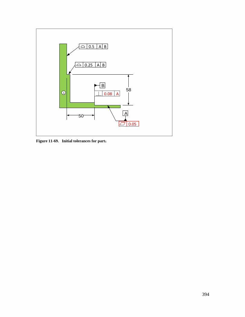
394

A

B

0.25 A B

0.5 A B

58

50

0.05

0.08 A1


395

Ø 0 A BM

Ø 0 A BM

Ø 45.0 – 45.4

75

30

Ø 44.0 – 44.4

88

25

A

B

B A

0.05

0.05

0.08 A

0.08 A

2

3


Graphical Method

Figure 11-71 shows the sketch assembly of the problem. The two fit features are

modeled at their MMC limit of size. Since the position tolerances are zero at MMC, the

actual positions of the fit features match their theoretical positions of 75 mm and 30 mm

for the hole and 88 mm and 25 mm for the pin. The surfaces that support the fitting parts

are controlled by profile tolerances. The profile-controlled surfaces are set to their

maximum values of 50.25 mm for the lower step and 58.125 mm for the upper step.

Based on these dimensions, the distance between the centers of the two fit features

becomes 0.28 mm. The minimum gap between the two fit feature surfaces becomes 0.02

mm as indicated in the sketch.

396

Figure 11-71. The sketch assembly of the problem

Figure 11-72 shows the detailed view of the fit features and the minimum gap. The

minimum gap is located along the line connecting the centers of the fit features.

397

Figure 11-72. The resulting minimum gap between the fit features is 0.02 mm

In order to set the minimum gap to zero we can increase the size of the pin feature by

0.04 mm from 44.4 to 44.44 mm. Note that the gap is a radial dimension while the

feature size is a diametrical value.

Figure 11-73 shows the 3D model of the assembly, the minimum gap in the fit and the

center distance between the fitting features.

398

Figure 11-73. The 3D model of the assembly showing the distance between the fitting feature centers

and the minimum gap value.

The CAD system finds the minimum distance between two circular feature profiles. In

this case the gap value of 0.02 mm and the center distance value of 0.28 mm are in

agreement with the sketch assembly solution.

Example-11: Analysis of fits with simultaneous fit features

Figure 11-74 shows a four-part fit assembly that was discussed in Chapter-10. Part4 has a

pattern of two holes fitting two boss features of the side parts. Assume the side parts are

glued to the bottom plate.

399

part1

part3

part2

part4

Figure 11-74. A four-part assembly

Figure 11-75 shows the feature and tolerances for part1.

2X 12.1 – 12.2

A

0 AM

A0.3 L 0.05

INDIVIDUALLY

80

1

Figure 11-75. Initial tolerances of part1

Figure 11-76 shows the feature and tolerances for part2 and part3.

400

A

0 AM

M L0.3 A B

12.0 – 12.1B

9.0 – 9.1

0.05

2 3


Figure 11-77 shows the feature and tolerances for part4 bar that is placed last into the

assembly.

2X Ø 9.5 – 9.6

Ø 0 M

96

4


401

Graphical Solution

Since the bar has two simultaneous fits, we have to set up the problem such that two gaps

are to be checked together. Multiple gap formulations become more complex to solve

manually but fortunately such multi-gap problems can often be avoided. In this case we

select the hole sizes to be slightly bigger than boss sizes such that each can individually

fit to its mating boss. The hole on the right fits first and becomes a constraint for the fit

of the hole on the left. We must now analyze the fit of the left hole and the left boss.

Figure 11-78 shows the arrangement of parts for fit.

Gap

Figure 11-78. Worst-case arrangement of parts for fit

To set up this fit problem graphically for minimum gap check, we can develop the

tolerance loop and use that as a guide for setting the dimension limits that minimize the

gap. However, in many cases we can intuitively deduce the dimension limits that lead to

a minimum gap. In this case we model the features such that the pins are farthest apart

and the holes are closest to each other. The slot and rail sizes are modeled at the LMC

limit of limit of size. The hole and pin sizes are modeled a their MMC limit of size. The

following list summarizes the modeling selections:

The slots will be modeled at their LMC size limit of 12.2 mm

The slots will be located at a distance of 0.3 mm larger than the basic distance

between the slot center planes.

The rails will be modeled at their LMC limits of size of 12.0 mm.

The bosses will be at their MMC limits of size of 9.1 mm.

The bosses will be located 0.15 mm off their theoretical positions because of the

0.3 mm position tolerance at MMC specification. The right boss is 0.15 mm to

the right and the left boss is located 0.15 mm to the left.

402

The holes will be at their MMC limits of size of 9.5 mm

The holes will be located at their theoretical distance because of the zero position

at MMC specification.

Figure 11-79 shows the 3D model of the assembly created with the design dimensions

and tolerances.

Figure 11-79. The 3D model of the assembly

The assembly is built in the worst-case arrangement where the two side parts are pushed

away from each other. The bar’s right hole is made tangent to the right boss. The

minimum gap is then checked in the left hole/boss fit. Figure 11-80 shows the result of

the checking the gap. In this case the minimum gap is actually 0.4 mm of interference.

403

Figure 11-80. The minimum gap is 0.4 mm of interference

In order to set the minimum gap to zero we can increase the size limits of the two holes

by 0.4 mm to 9.9 – 10.0 mm.

Analytical Solution

Figure 11-81 shows the tolerance loop for the fit analysis of the gap. There are four pairs

of fits numbered one through four. Each fit includes a ½ H vector and a ½ F vector.

There are also four position dimensions. The F vectors are shown in blue while the H

vectors are shown in red.

404

G

Aa Ba

Da

1

2 3

4

Ca

1

4

23

Figure 11-81. The tolerance loop for predicting the minimum gap size

The axes and center planes referenced are the actual axes and center planes.

Aa : Connects the boss axis to the rail center plane on part2

Ca : Connects the boss axis to the rail center plane on part3

Ba : Connects the center planes of the rails on part1

Aa : Connects the axes of the two holes on part4

The gap expression can be developed by simply following the arrows as they start from

the head of the gap vector going around the loop ending at the tail of the gap vector

G + (½ F1a + Aa) - ½ F2a + (½ H2a + Ba + ½ H3a) - ½ F3a + (Ca + ½ F4a)

- (½ H4a + Da + ½ H1a) = 0


Gmin = (½ H4a + Da + ½ H1a)min - (Ca + ½ F4a)max - (½ H2a + Ba + ½ H3a)max

- (½ F1a + Aa)max + (½ F2a)min + (½ F3a)min

The holes have zero position at MMC specification, therefore

(½ H4a + Da + ½ H1a)min = ½ (9.5) + 96 + ½ (9.5) = 105.5

The pins have 0.3 mm position tolerance at MMC

(Ca + ½ F4a)max = 8 + ½ (0.3) + ½ (9.1) = 12.7

(½ F1a + Aa)max = 8 + ½ (0.3) + ½ (9.1) = 12.7

The slots have 0.3 mm position tolerance at LMC

(½ H2a + Ba + ½ H3a)max = ½ (12.2) + (80 + 0.3) + ½ (12.2) = 92.5

The minimum gap becomes

Gmin = 105.5 – 12.7 – 92.5 – 12.7 + ½ (12) + ½ (12) = - 0.4 mm

The result agrees with the graphical solution.

405


gap of zero. The gap expression is

G = (½ H4a + Da + ½ H1a) - (Ca + ½ F4a) - (½ H2a + Ba + ½ H3a)

- (½ F1a + Aa) + (½ F2a) + (½ F3a)

The basic position dimensions sum up to zero and are not entered as an input vector

M = D – C – B – A = 96 – 8 – 80 – 8 = 0

The simplified gap expression has the following terms

G = ½ H4a + ½ H1a - ½ F4a - ½ H2a - ½ H3a - ½ F1a + ½ F2a + ½ F3a

The data for these terms are then entered in the program in the order they appear above.

Figure 11-82. The result of TAP worst-case analysis and statistical simulation

Exercise Problems

Problem-1

Consider the three part assembly shown in Figure 11-83. Model these parts in a CAD

system and dimension and tolerance the parts to be suitable to acheive a precision gap

performance. For reference, use 100 mm for the width of slot in part3. The rest of the

dimensions are up to you. The gap is to be between 1 mm and 1.25 mm. Assume

precisions to be consistent with milling processes. Only specify tolerance statements

relevant to the three-part fit. Use both graphical and analytical methods to set Gmin=1

mm. If necessary, only modify the width dimension of part3. Check the resulting

maximum gap against 1.25 mm limit. If the gap exceeds 1.25 mm, reduce the tolerances

and solve the problem again with reduced tolerance values. Verify the final results with

TAP.

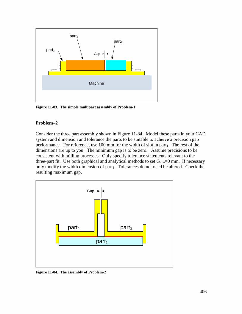
406

part3

Machine

part1

part2

Gap

Figure 11-83. The simple multipart assembly of Problem-1

Problem–2

Consider the three part assembly shown in Figure 11-84. Model these parts in your CAD


performance. For reference, use 100 mm for the width of slot in part1. The rest of the

dimensions are up to you. The minimum gap is to be zero. Assume precisions to be

consistent with milling processes. Only specify tolerance statements relevant to the

three-part fit. Use both graphical and analytical methods to set Gmin=0 mm. If necessary

only modify the width dimension of part1. Tolerances do not need be altered. Check the

resulting maximum gap.

part1

part2 part3

Gap

Figure 11-84. The assembly of Problem-2

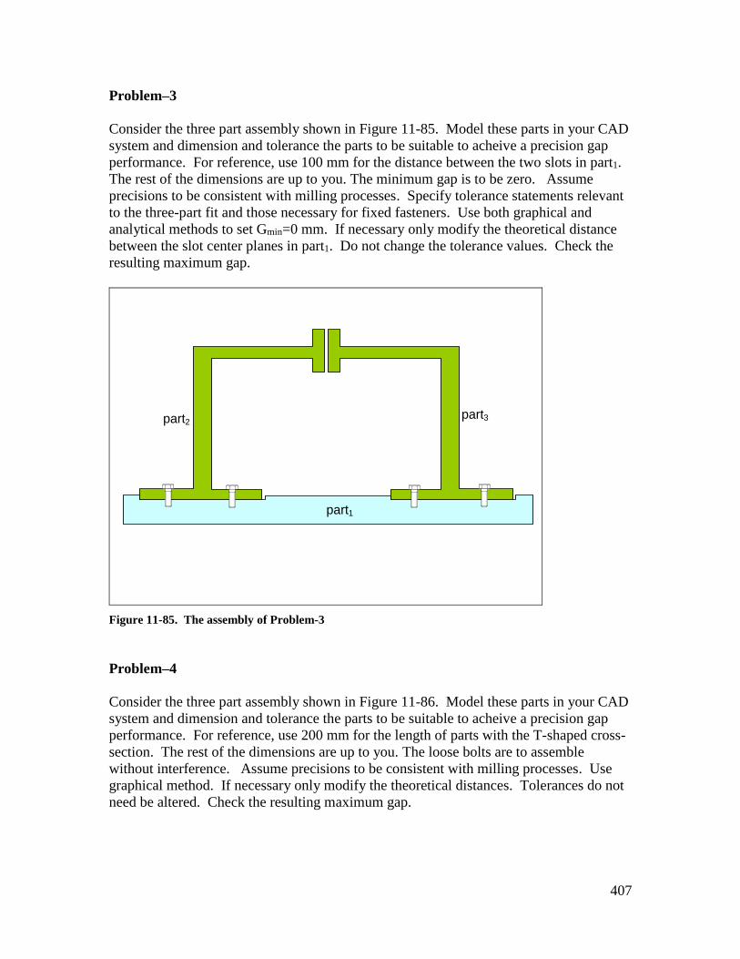
407

Problem–3



performance. For reference, use 100 mm for the distance between the two slots in part1.

The rest of the dimensions are up to you. The minimum gap is to be zero. Assume

precisions to be consistent with milling processes. Specify tolerance statements relevant

to the three-part fit and those necessary for fixed fasteners. Use both graphical and

analytical methods to set Gmin=0 mm. If necessary only modify the theoretical distance

between the slot center planes in part1. Do not change the tolerance values. Check the

resulting maximum gap.

part1

part3part2


Problem–4



performance. For reference, use 200 mm for the length of parts with the T-shaped cross-

section. The rest of the dimensions are up to you. The loose bolts are to assemble

without interference. Assume precisions to be consistent with milling processes. Use

graphical method. If necessary only modify the theoretical distances. Tolerances do not

need be altered. Check the resulting maximum gap.

408


409

INDEX

A

actual mating envelope ................................................................................................................................ 63 Angularity ..................................................................................................................................................... 70 arrangement ............................................................................................................................................... 370

B

bonus tolerance .......................................................................................................................................... 168

C

Circularity ..................................................................................................................................................... 56 Cylindricity .................................................................................................................................................... 58

D

datum feature simulators ............................................................................................................................. 59 datum features ............................................................................................................................................. 59 Dimensional tolerances ................................................................................................................................ 46

F

feature .......................................................................................................................................................... 16 features-of-size ............................................................................................................................................. 46 fit boundaries.............................................................................................................................................. 156 fit formula ................................................................................................................................................... 162 fixed fastener formula ................................................................................................................................ 270 Flatness ......................................................................................................................................................... 50 floating fastener formula ........................................................................................................................... 273

G

Geometric tolerances ................................................................................................................................... 47

I

independency symbol ................................................................................................................................. 226

M

maximum play formula .............................................................................................................................. 162

O

orientation-constrained actual mating envelope ....................................................................................... 217

P

Parallelism .................................................................................................................................................... 61 Perpendicularity ........................................................................................................................................... 67 presumed order of assembly ...................................................................................................................... 297 primary orienting datum surface ................................................................................................................ 230 projected tolerance zone ............................................................................................................................ 269

R

regardless of feature size (RFS) .................................................................................................................. 167

S

secondary orienting/locating surface ......................................................................................................... 230

410

staging .......................................................................................................................................................... 62 Straightness .................................................................................................................................................. 55

T

Tolerances of form ....................................................................................................................................... 50 Tolerances of orientation ............................................................................................................................. 59

U

unconstrained actual mating envelope ........................................................................................................ 63

V

virtual boundaries ....................................................................................................................................... 158

411

ISBN 978-0-9914638-0-0

applications of geometric tolerancing to machine design

Documents