Lattice Boltzmann schemes for convection-diffusion phenomena;

application to packages of agricultural products

R.G.M. van der Sman

Promotoren:

dr.ir. G.P.A. Bot hoogleraar in de Technische natuurkunde, Landbouwuniversiteit Wageningen

dr. M.H.J.J. Ernst

hoogleraar in de Theoretische natuurkunde, Universiteit Utrecht.

Co-promotor:

dr. J.H.J, van Opheusden

universitair docent, departement Agro-, Milieu- en Systeemtechniek, Landbouwuniversiteit Wageningen

Stellingen bij het proefschrift:

Lattice Boltzmann schemes for convection diffusion phenomena; application to packages of agricultural products

R.G.M. van der Sman, Wageningen, 7 mei 1999.

1. Door de integrate beschouwing van fysica, kwaliteitsverloop en logistiek ontstijgt het ontwerpen van transportverpakkingen van agrarische producten het basale niveau van de huidige heuristiek: "Stans er maar gaten met 5% openingspercentage in", waardoor een significante verbetering van het kwaliteitsbehoud te bereiken valt.

M.T. Talbot and CD. Baird, Evaluating commerical forced-air pre-coolers. ASAEpaper 91-6021. 1991.

2.Vanuit het beginsel dat de hydrodynamische momenten van de evenwichtsverdeling gelijk moeten zijn aan die van de Maxwell-Boltzmann verdeling, zijn Lattice Boltzmann schema's volledig afleidbaar.

(In dit proefschrift)

3. De Lattice Boltzmann methode wordt een gelijkwaardige concurrent van de standaard discretisatie-methoden van fysische transportvergelijkingen door de introductie van schema's voor onregelmatige roosters.

(In dit proefschrift)

4. Door discretisatie van transportverschijnselen op het niveau van de fysische beschrijving, vermijdt men de complicaties die gepaard gaat met de formele discretisatie van partiele differentiaal vergelijkingen voor continue modellen.

5. De Darcy-Forchheimer vergelijking geeft ook in het turbulente regiem bij Re>300, waar Anthone afwijkingen verwacht, een correcte beschrijving van luchtstroming door gestorte of gepakte groenten en fruit.

B.V. Anthone and JL Lage. A general two-equation macroscopic turbulence model for incompressible flow in porous media. Int. J. Heat Mass Transfer 40 (13): 3013-3024 (1997).

6. De gangbare denkwijze in de verpakkingswereld dat ventilatiegaten in de wanden van verpakkingen voor agrarische producten afbreuk doet aan de mechanische sterkte, gaat in veel praktijksituaties niet op.

7. De ASTM-testen voor de mechanische sterkte hebben een beperkte voorspellende waarde voor de praktijksituaties van verpakkingen voor agrarische produkten, die gekenmerkt worden door lage temperaturen en hoge luchtvochtigheid.

8. Voor plezier en succes in de wetenschap dient men te beschikken over een goede portie juveniliteit.

9. Ontologische aberraties induceren cognitieve congestie.

^ M Q S ^ , ^ l S

R.G.M. van der Sman

Lattice Boltzmann schemes for convection-diffusion phenomena; application to packages of agricultural products

Proefschrift ter verkrijging van de graad van doctor op gezag van de rector magnificus van de Landbouwuniversiteit Wageningen, dr. CM. Karssen, in het openbaar te verdedigen op vrijdag 7 mei 1999 des namiddags te 13.30 uur in de Aula.

\TW^ °y &Z\C5

CIP-DATA KONINKLIJKE BIBLIOTHEEK, DEN HAAG

Sman, van der, R.G.M. Lattice Boltzmann schemes for convection-diffusion phenomena; applica­tion to packages of agricultural products / R.G.M. van der Sman Thesis Wageningen. - With Ref. - With summary in Dutch. ISBN 90-5808-048-X Subject headings: Lattice Boltzmann / convection diffusion / packaging.

Copyright (c)1999 by R.G.M. van der Sman

Cover: Simplifying the physics in packages by a ball game, (c) R.G.M. van der Sman

BIBLIOTHEEK LANDBOUWUNIVERSITF.IT

WAGENINGEN

Voorwoord

Dit proefschrift is geschreven op basis van mijn onderzoek bij het agrotech-nologisch onderzoeksinstituut ATO-DLO. Dit onderzoek is financieel mo-gelijk gemaakt door: het ministerie van Economische zaken; SCA Pack­aging Tilburg; poot-aardappelexporteurs Agrico, ZPC, en Hettema; Pro-ductschap voor Siergewassen; en ATO-DLO.

Dit proefschrift is mede tot stand gekomen dankzij vele mensen, die ik dank verontschuldigd ben voor hun begeleiding, motivatieen ondersteuning.

Allereerst wil ik mijn (co)-promotoren, prof. G.P.A Bot, prof. M.H. Ernst, dr. J.H.J, van Opheusden bedanken voor hun begeleiding, inhoudelijke bijdrages en het vervolmaken van de publicaties.

Evenzo hebben mijn begeleiders bij ATO-DLO, dr. R.G. Evelo, dr.ir. J.M. Soethoudt, dr. A.C. Berkenbosch, een wezenlijke bedrage geleverd aan het feit, dat dit werk in een strak tijdschema gerealiseerd is. Zij, en tevens ook mijn collega dr.ir. J.J.M. Sillekens, hebben veelvuldig als klankbord gefungeerd, waar ik hen ook hartelijk voor dank.

Als laatste wil ik mijn dank en liefde betuigen aan mijn vrouw Gerlies en onze zoon Hugo, voor hun ondersteuning, motivatie en genegenheid. Zonder wanklank heb ik thuis immer de gelegenheid en ondersteuning gekregen om mijn proefschrift te schrijven. Evenzo belangrijk is de tijd geweest, die we gezamelijk doorgebracht hebben de afgelopen zeven jaar, waardoor ik dit werk toch ook opzij heb kunnen zetten.

Een speciale plek in mijn hart heeft mijn zoon Hugo, wiens blakende levensvreugde mij altijd goed doet. Daarom, draag ik dit boekwerk op aan Hugo.

Contents

Nomenclature 1

1. Introduction 5

1.1 Modelling physics of packed agricultural products 5

1.1.1 Packaging systems for fresh agricultural products 5 1.1.2 Physical processes in transport packages 7 1.1.3 Numerical methods 8 1.2 Lattice Boltzmann schemes 10 1.3 Scope of this thesis 15 1.4 Outline of this thesis 16

2. Cooling of packed cut flowers 19

2.1 Introduction 15 2.2 Convection-diffusion scheme with heat transfer 21 2.2.1 1-D convection-diffusion scheme 21 2.2.2 1-D convection-diffusion with source terms 21 2.3 Modelling the cooling of flowers 25 2.3.1 Initial and boundary conditions 28 2.3.2 Experiments 29 2.3.3 Simulation 32 2.4 Conclusions 33 Appendix A Chapman-Enskog procedure 34

3. Natural convection in a potato container 37

3.1 Introduction 37 3.2 Lattice Boltzmann scheme 39 3.3 Orthorhombic lattice 41 3.4 Boundary conditions 42 3.5 Analytical solutions 43 3.6 Experiments 44 3.7 Conclusions 46

4. Vent hole design of potato containers 49

4.1 Introduction 49 4.2 Problem description 50 4.3 Lattice Boltzmann schemes 53 4.3.1 Convection-diffusion 54 4.3.2 Porous media flow 55 4.3.3 Convective heat and mass transfer 55 4.4 LB scheme for heat and mass transfer

in seed potato containers 54 4.4.1 Boundary conditions 57 4.5 Condensation of moisture during cooling conditions 60 4.6 Numerical analysis of alternatie vent hole designs 62 4.7 Conclusions 65

5. Diffusion on an orthorhombic lattice 69

5.1 Introduction 70 5.2 Lattice Boltzmann scheme 70 5.2.1 Lattice Boltzmann Equation 70 5.2.2 Symmetries 71 5.2.3 Collision opearator 72 5.3 Eigenmodes analysis 75 5.3.1 Eigenmodes 75 5.3.2 General properties 75 5.3.3 Perturbation analysis 76 5.4 Optimisation of the DLB scheme 78 5.4.1 Free parameter K 78 5.4.2 Lattice spacing 81 5.5 Discussion 81

6. Convection-diffusion on irregular lattices 85

6.1 Introduction 85 6.2 LB scheme for orthorhomic lattices 87 6.3 LB scheme for irregular grids 89 6.4 Numerical analysis 92 6.4.1 Gradient resolution 93 6.4.2 Transient problems: method of moments 94 6.4.3 Transient problems:

comparison with traditional schemes 97 6.4.4 Transient problems: 2-D lattices 101 6.5 Discussion 102 6.6 Conclusions 104 Appendix A Relation with Finite Difference schemes 104

7. Concluding Remarks 107

Summary 111

Samenvatting 113

Curriculum Vitae 116

Nomenclature

Nomenclature of PDE models

a Agpec

C

Cp

D d

9 k K L

P Q r s S t T u X

y z

a

P e K

X V

P <T

thermal diffusivity specific transfer area vapour density specific heat diffusion coefficient thickness gravitational constant wave number Darcy's law coefficient length pressure volumetric heat production rate specific heat of evaporation relaxation rate volumetric mass production rate time temperature velocity spatial co-ordinate spatial co-ordinate spatial co-ordinate

heat transfer coefficient mass transfer coefficient porosity permeability heat conductivity kinematic viscosity mass density variance of Gaussian distribution

[m2.s-1} [m2.m-3] [kg.m~3] [J.kg-'.K'1] [m2.s-1] [m] [m.s-2] [m-1]

[s] [m] [N.m-2] [W.m-3] [J-kg-1]

is'1} [kg.m 3.3 1]

w [K] [m.s-1] [m] [m] [m]

[W.m~2.K] [m.s-1]

H [m2] [W.m-KK-1] [m'.s-1] [kg/m-3] [m]

2 Nomenclature

Nomencla ture of LB schemes

A Ci

cs

D e

f, 9> hi H

J k Ni Pe'

9. s S

u Vi

Va,i

V Wi

4> $

r A

A< A*a

P

c u> CI

collision operator propagation speeds speed of sound diffusion coefficient unit vector number density of fluid particles number density of lattice gas particles number density of heat particles in air Hermite tensor polynomial particle flux wave number number of lattice gas particles grid Peclet number = uAx/D number density of heat particles relaxation rate surface area of Wigner-Seitz cell Courant number = uAt//\x distribution of vapour lattice gas particles eigenvector volume of Wigner-Seitz cell weight factor transfer rate transfer operator mass flow eigenvalue Knudsen number eigenvalue density of lattice gas particles angle relaxation rate collision operator

Nomenclature

Super- and subscripts

a A c eq ext

f 9 h i int m

w p 1 sat tot V

w 0 1

air general physical quantity, e.g. cardboard equilibrium external fluid particles generic lattice gas heat particles in air state index internal condensed moisture n-th order perturbation product heat particles saturated total vapour particles water content of product ambient condition initial condition

heat or mass

Chapter 1

Introduction

1. Modelling physics of packed agricultural products

1.1. Packaging systems for fresh agricultural products.

For marketing fresh agricultural and horticultural products, quality con­servation is of great importance. Packaging is crucial for maintaining the product quality in the distribution chain. The primairy function of the package is the prevention of mechanical damage. Furthermore, the package should act as a barrier between the inside and outside climate conditions. As a barrier, the package protects its contents from hazardous outside con­ditions and enables the development of a favourable microclimate inside. The microclimate, favourable for most products, has a low temperature, a high, non-condensing humidity (90-95% R.H.), and a low ethylene level. Furthermore, an atmosphere with modified oxygen and carbon dioxide lev­els is beneficial for the quality of a wide range of fruits, vegetables and flowers1.

Hence, the exchange of heat, water vapour and gasses of the packaging system with the environment must be carefully controlled. Due to the large differences in physiological behaviour of agricultural products and physical conditions in the distribution chains, the package design must be tuned to each specific combination of packaged product and distribution chain. How to tune the packaging design optimally to the specific needs, is still not thoroughly understood. Many empirical studies have shown that existing packaging design can be further improved1-6 .

It has been recognised that the process of designing packaging systems can be greatly improved by the use of a computer model based approach1.

6 Chapter 1

By means of computer models certain physical and physiological phenom­ena in the packed bed of products can be calculated, whereby packaging properties and the environmental conditions can be changed quite easily. Having acquired the knowledge of the products behaviour in various pack­age systems and conditions, the packaging design can be optimised for the quality of the packaged product. By using a computer model, the im­provements of packaging design can be obtained much faster and with less expenses than by using pure empirical studies.

Wi th success, computer models have been used for the design of retail packages of fresh agricultural p roducts 1 . Retail packages They are mostly wrapped in plastic foils, which control the exchange of gas and water vapour with the environment and thereby create a modified atmosphere. Conse­quently, they are called Modified Atmosphere packages. The dominant physical process is gas diffusion through the foil. I ts interaction with the respiration of the packaged product creates the modified a tmosphere.

In retail packages, containing a small amount of product (less than one kilogram), one can expect little spatial variation in the physical and physiological conditions. Hence, the physical processes in retail packages can be described by ordinary differential equations, which normally pose little mathemat ical difficulties1.

Contrary to retail packages, the spatial variation of physical quantities t ransport packages, containing 1 to 1000 kg of product , can be signifi­cant and result in spatial variation in product quality. Therefore, in the computer models one has to account for the spatial distribution of physi­cal quantities, which is mathematically described with partial differential equations.

In most t ransport packages the heat and water vapour exchange are con­trolled by vent holes, which allow air flow through the package. Hence, the dominant physical processes are the flow of air and convection-diffusion of heat and water vapour. The numerical modelling of the spatial distribution of t emperature and humidity driven by convection-diffusion is ra ther com­plex, and as a consequence only a very few numerical studies have been done on physical t ransport phenomena in packaging systems with vent holes7 .

However, considering the presently available computer power and the variety of numerical methods, we believe tha t modelling of physical pro­cesses in t ransport packages is feasible. Therefore, in this thesis we will focus on the modelling of physical phenomena as a design tool for t rans­port packages of fresh agricultural products.

Introduction 7

1.2. Physical processes in transport packages.

In transport packages with vent holes, the exchange of temperature and humidity with the environment is mainly driven by airflow. This airflow is caused by forced ventilation driven by a fan system or by natural ventilation induced by air density gradients. The rate of ventilation depends on a range of factors: the outside pressure conditions; temperature differences between the inside and outside of the package; the size and location of the vent holes; and the often intricate geometry of the packaged product. In most cases, the dependence of the ventilation rate on these factors can only be found by numerical studies.

The ventilation problem can be simplified by assuming that packed beds of agricultural products can be described as porous media. In this approach the full details of the flow are not conidered, but the volume-averaged flow is described. The volume averaged flow follows Darcy's law:

pu = -KVp. (1.1)

This law states that the mass flow pu is only due to a pressure gradient Vp. For small flow velocities, as occur during natural ventilation, the coefficient K is only dependent on the geometry of the packed bed and the hydrody-namic properties of the fluid phase. In situations of forced ventilation with Reynolds number Re > 1, inertial effects of the air flow become important, leading to a velocity dependence of the coefficient8, i.e., K = K{u) . In that case, the airflow is described by the so-called Darcy-Forchheimer equation.

The exchange of heat and water vapour of the packaging system with the environment can mathematically be described by the so called convection-diffusion equation:

dtCA + U-VcA = DAV2CA + SA. (1.2)

Here cA represents the density of the conveyed physical quantity A, e.g., heat or water vapour, DA is the diffusivity of the physical quantity A in the porous medium, 5,4 is a source term representing the production or consumption of the quantity A, which can be due to evaporation, conden­sation, respiration, or heat and mass transfer between the packaged product and the air flow.

Solving the convection-diffusion equation numerically is a complicated matter, in which many of the conventional numerical methods have proven to be unsatisfactory9. Results adequate for engineering problems can be obtained with numerical schemes10,11'12, which require highly specialised knowledge of numerical mathematics.

The practice of packaging for agricultural products demands that the model based approach can handle the design question for a variety of pack-

8 Chapter 1

aged products and outside conditions. Moreover, the design question should be solved in a comparatively short period. This situation calls for a numer­ical method which can handle the various physical phenomena occurring in packaging systems within a single framework and poses few mathematical difficulties. We have found a very promising framework in one of the newly developed methods in computational physics.

1.3. Numerical methods.

Conventional numerical methods for solving physical transport phenom­ena are based on the continuum concept, which assumes that all matter is continuously distributed over space. Physical quantities are mathematically described by fields. The evolution of fields in time is described mathemat­ically by partial differential equations, such as Eqs.(l.l)-(1.2). In order to obtain a numerical solution, the partial differential equations have to be discretised on a computational grid. The most frequently applied dis­cretisation methods are the Finite Difference, Finite Volume and the Finite Element methods.

Difficulties arise with the straightforward application of these methods to problems as convection-diffusion and free fluid flow, when the convective flux exceeds the diffusive flux. These regimes are identified by a high Peclet number, which is defined as Pe = uL/D with L a macroscopic length scale. At high Peclet numbers, steep spatial gradients in the physical quantities can occur near system boundaries. In order to get a proper approxima­tion of the spatial derivative in regions with steep gradients, the grid must be sufficiently refined. If the grid is not refined enough or the time step is too large, the steep gradients will induce spurious oscillations (wiggles) or even numerical instabilities. For convection-diffusion phenomena with high Peclet numbers the remedy of refining the mesh and reducing the timestep ceases to be practical. To overcome the problem special discreti­sation schemes must be applied10,11,12, which in most cases introduce some form of artificial diffusion to damp these spurious oscillations. A specialised branch of numerical mathematics has developed trying to find these special discretisation schemes.

In response to the difficulties inherent to the conventional numerical schemes for convection-diffusion, alternative methods are developed which leave the continuum concept. Motivated by the fact that in reality all physical transport phenomena, as fluid flow and convection-diffusion, are a pure consequence of the movements and collisions of molecules, the so-called particle methods have been developed13-17.

In these methods one lumps matter in giant quasi-particles, carrying portions of the macroscopic physical quantity such as heat, mass, vorticity

Introduction 9

or an amount of a chemical species. The kinetics of these quasi-particles resembles largely that of real molecules: they propagate according to their speed, interact with each other through collisions and can be accelerated by external force fields. This resemblance of particle methods with the molecular micro-world makes them quite appealing to physical intuition.

In various particle methods the kinetics is further simplified by discretis-ing space and/or particle velocity. Examples of particle methods are the gradient particle methods13,14, Dissipative Particle Dynamics (DPD)15 '16, Smooth Particle Dynamics (SPD)17, Lattice Gas Automata and Lattice Boltzmann (LB) schemes21-26 . The latter methods are the most simplified of all, as time, space and particle velocity are discretised. Because of this simplicity they have attracted a lot of attention during this last decade.

In figure 1.1, we have depicted the views of the continuum and par­ticle concepts towards the modelling of macroscopic phenomena and the mapping of the concepts to the computational domain.

The ease of handling convection-diffusion problem with particle methods originates from their Lagrangian nature. Steep gradients and interfaces be­tween immiscible fluids move automatically with the propagating particles. This is in contrast with the Finite Difference or Finite Element method, in which steep gradients and interfaces have to be tracked explicitly.

A very successful particle method is the Lattice Boltzmann method. This method has shown to be able to model a variety of complex macro­scopic phenomena such as Navier-Stokes flow26, multi-phase flow27,28, porous media flow29 and natural convection30. Motivated by the successes of the Lattice Boltzmann scheme in describing complex physical phenomena we have chosen it as the framework for modelling of physical transport phe­nomena occurring in packaging systems.

The Lattice Boltzmann method seems to meet all our demands as a modelling tool for physical processes in packaging systems. It uses a single and simple paradigm of colliding particles on a grid, for the description of various physical phenomena. Furthermore, new applications are expected to be implemented in a short time without much difficulty. In this thesis, we will investigate whether these promises indeed hold for the Lattice Boltz­mann method. This investigation is mainly focussed on the convection-diffusion phenomena occurring in packages of fresh agricultural products. In addition, we study the effectiveness of the Lattice Boltzmann method by comparing it with conventional numerical methods using benchmark problems.

10 Chapter 1

Figure 1.1: Modelling of real macroscopic phenomena according to particle and continuum concepts.

2. Lattice Boltzmann schemes

Taking the ideas of particles methods and cellular automata20, Lattice Gas Automata (LGA) and Lattice Boltzmann (LB) schemes model phys­ical phenomena with quasi-particles. These so-called lattice gas particles move and collide on a regular lattice. The collisions are according to rules, which obey appropriate conservation laws such as for mass, momentum and energy. Despite the simple dynamics of the lattice gas particles, these methods have shown to be able to describe many complex hydrodynamic phenomena. Examples of these phenomena are vortex shedding and in-terfacial instabilities. In LGA and LB schemes these complex phenomena simply emerge from the collective behaviour of a large collection of lattice gas particles21. It is shown that the only prerequisites for applying LGA

Introduction 11

and LB schemes to fluid dynamics are 1) conservation of mass and mo­mentum by the collisions, and 2) a sufficient lattice symmetry to ensure isotropy of the fluid dynamics.

The locations of the lattice gas particles are restricted to lattice sites only, such that in effect the lattice gas particles only have a discrete set of velocities {c,}. The physical state of the Lattice Gas Automaton is deter­mined by the particle distribution function of lattice gas particles <7,(x,<), which denotes the number of particles moving with velocity c,- at the lattice site x and time t. Lattice Gas Automata allowfifj(x, t) to take only Boolean values, whereas the Lattice Boltzmann method puts no restriction on the values of gi(x,t).

Pre-collision t=t*-1

Figure 1.2: Lattice gas particles on a hexagonal lattice, colliding at time t = t*. the collisions obey the conservation laws of mass and momentum.

Macroscopic physical quantities, such as mass and momentum densi­ties, are derived by taking moments of the particle distribution function.

12 Chapter 1

For example for a fluid, the mass density is p(x,t) = £I»5«(X>0 and the momentum density is p(x,t)u(x,t) = J2i Cj#i(x,<). The lattice gas par­ticles evolve in two steps: a collision step and a propagation step. Due to collisions the particles are scattered over all directions, leading to the post-collision distribution function:

5,'(x>') = £ ^ ( x , < ) . (1.3)

The elements of collision matrix A{j denote the probability of a particle for the transition of propagation direction j to direction i. These transition rates must account for the conservation laws, such as conservation of mass. Thus, this law imposes that Yli9i(K>t) = Yli9i(x>t)-

After collision, the particles propagate to adjacent lattice sites according to their velocity:

(/.•(x + CiAt,t + At) = gfct). (1.4)

This process of collision and propagation is illustrated in figure 1.2 for a Lattice Gas Automaton modelling fluid flow.

Due to the restriction of gi(x,t) to Boolean values, Lattice Gas Au­tomata have some drawbacks. The macroscopic physical quantities show a very noisy behaviour in time and true fluid dynamic behaviour is obtained only for low Reynolds and Mach numbers. These limitations have been remedied by the introduction of the Lattice Boltzmann method 23, which allows <7;(x,£) to have real numbered values. Soon after the introduction, a rapid development of the research field has followed. LB-schemes have been applied to a variety of complex phenomena, as mentioned above and in the recent review by Chen31.

Their success can be accounted to two factors: 1) the ability to han­dle complex boundary conditions with simple collision rules, and 2) the suitability of the local collision rules to calculation by massively parallel computers.

Altogether, the Lattice Boltzmann method has very attractive proper­ties, which make it suitable as a modelling framework for transport phe­nomena in packaging systems. These properties are summarised below:

• Within the single framework of the LB method, a variety of physical processes can be modelled.

• Complex phenomena as convection-diffusion and fluid flow can be modelled by straightforward application of the standard Lattice Boltz­mann algorithms.

Introduction 13

• New phenomena are easily incorporated within the framework of the LB scheme. The required particle kinetics can be derived using physi­cal intuition. Highly specialised knowledge of numerical mathematics is not required.

• Due to their simplicity, LB schemes are easy to implement.

However, there are still some limitations to the LB method, which reduce its competitiveness with respect to convential numerical methods in solv­ing engineering problems. These limitations are 1) the Lattice Boltzmann method is restricted to regular lattices, and 2) there is no sound mathemat­ical foundation for deriving LB schemes for new physical phenomena. The Finite Element and Finite Difference method do not have these limitations; they can refine their grids in regions with steep gradients and in princi­ple they can model any physical process which can be described by partial differential equations, using a clear mathematical discretisation procedure.

The limitations of the Lattice Boltzmann method may restrict the num­ber of applications in the field of transport packaging systems. For ex­ample, in packaging systems with air flow through small holes driven by forced ventilation, high gradients in the flow velocity can occur, which can only be solved efficiently with grid refinements32. By the lack of a mathematical foundation it is unclear how to describe phenomena like Stefan-Maxwell (multi-component) diffusion, as occur in bulk Modified-Atmosphere packages33.

These limitations of the Lattice Boltzmann method are recognised34. Consequently, several studies on LB schemes for irregular grids have been performed35-37. However, do not obey conservation laws, increase numer­ical diffusion and above all, they have lost the simplicity, which makes the LB method so attractive. Other studies have been performed, investi­gating the theoretical basis of the LB method25,28 '38. These studies have achieved some important progress, but a complete theoretical framework is still missing.

All the above mentioned studies, directed to irregular grids or to the theoretical framework of the LB method, are concerned with complex phe­nomena like Navier-Stokes flow or multi-phase flow. However, the phenom­ena in transport packaging systems, such as convection-diffusion and Darcy flow, are more simple, physically speaking. Hence, they represent better test problems to investigate whether the limitations of the LB method can be lifted.

14 Chapter 1

Application

Physics

Physical Transport Phenomena

/ \

^

Conceptual Models

/

)

/ t Continuum / . 1 d^scnptiort 1

i

M Particle

description

\

\

Finite Djflejence / • »ethod / I

Lattice Boltzmann schemes

Figure 1.3: This thesis positioned in related fields of research. Unhatched blocks represent the topics of this thesis. Hatched blocks represent directly related top-

Introduction 15

3. Scope of this thesis

In this thesis, a model based approach is developed for the description of convection-diffusion processes, as occur in transport packaging systems for fresh agricultural products. The computer models considered will be based on the Lattice Boltzmann (LB) scheme. This is a recently developed numerical method, which uses a particle description of physical transport phenomena, as described in the previous section. How the topics of this thesis can be positioned in related fields of research, is displayed in figure 1.3.

The focus of this thesis is the investigation of the feeasibility and effec­tiveness of the LB scheme in modelling convection-diffusion phenomena in applications of packaging systems. This is done in three ways:

• New LB schemes are developed and tested for several convection dif­fusion problems, taken from the practice of packaging systems for agricultural products.

• The solution of physical problems, which are new to the existing framework of LB schemes, is investigated analytically and numeri­cally.

• The developed LB schemes are compared with conventional numerical methods using benchmark problems.

The applicability of the LB scheme to modelling physical processes in packaging systems is tested by using it for package design problems in research projects. These project are performed at the Agrotechnological Research Institute ATO-DLO. The testing of the LB schemes is performed by comparing simulation results with experimental data, which are obtained within research projects at ATO-DLO.

In order to be able to model various other phenomena such as heat transfer, ventilation through holes, evaporation and condensation, porous flow with buoyancy, various new collision rules and boundary conditions have to be devised. As the kinetics of the lattice gas particles mimics the underlying physical process, the necessary extensions of the LB scheme can be developed using physical intuition. This is a valuable asset of the LB scheme if design problems have to be solved in a short period of time. However, because of the rather intuitive procedure for constructing new collision rules and boundary conditions, the applicability of these new rules still has to be validated by solving benchmark problems.

As discussed in the previous section, it is stated that in order to be a competitive modelling tool, the limitations on the Lattice Boltzmann scheme must be relaxed, i.e., the restriction to regular grids and the lack

16 Chapter 1

of a mathematical framework. Therefore, we investigate in this thesis, whether these limitations can be lifted for convection-diffusion, which is the dominant physical process in transport packaging systems with vent holes. This will be the topic of the latter part of this thesis.

Finally, the performance and the competitiveness of the Lattice Boltz-mann schemes is compared with that of conventional numerical schemes. This is investigated by solving several benchmark problems.

4. Outline of this thesis

In Chapter 2, we present the first test case problem for which we test the applicability of the LB-scheme in modelling convection-diffusion phe­nomena. The case considered is that of pre-cooling of packaged cut flow­ers. This problem involves convection-diffusion with simultaneous heat and mass transfer. It is a very suitable first test case, since it can be treated as a one-dimensional problem with a uniform and constant flow field.

A more complex test case is the heat flow in a package, that is driven by natural convection. This test case is studied in Chapter 3. The test case concerns a bulk potato package, whose contents can be treated as a porous medium. A three-dimensional LB scheme is developed with new collision rules for porous flow driven by buoyancy. The LB scheme is tested with data obtained from experiments performed with closed potato containers. New boundary conditions are formulated for modelling the heat conducting walls of the containers.

An actual package design problem is addressed in Chapter 4, in which we seek a vent hole design for a bulk potato package. The vent hole design must ensure an optimal water vapour exchange with the environment, and thereby it must prevent condensation of moisture on the potatoes. The LB scheme from the previous chapter has been extended for modelling the mass transfer, the condensation and the ventilation through the holes in the walls of the potato container.

In search of a theoretical framework for the Lattice Boltzmann method, we present a procedure for constructing a diffusion scheme from first princi­ples in Chapter 5. By applying this procedure, we study ways to generalize and optimize the (diffusion) LB scheme. The performance of the generalized and optimised LB schemes concerning consistency, stability and accuracy are investigated with eigenmodes analysis.

The procedure, which we have developed in Chapter 5, is extended and applied to convection-diffusion schemes and is described in Chapter 6. Gallilean invariant schemes are constructed for Bravais lattices. Further­more, we show that by using a similar procedure, LB schemes for irregular grids can be derived. The efficiency of these new LB schemes are compared

Introduction 17

to t ha t of Finite Element and Finite Difference schemes. This thesis concludes with a discussion about the use of computer mod­

els, and in particular the Lattice Boltzmann schemes, for solving convection-diffusion problems in packaging systems of fresh agricultural products. As we have extended the LB methodology with new boundary conditions and irregular grids, their potential use for solving physical problems in general will be discussed too. In addition directions for further research in the field of modelling physical processes in packaging systems will be given.

1. A.A. Kader, D. Zagory, and E.L. Kerbel, Modified atmosphere packaging of fruits and vegetables. Crit. Rev. Food Nutr., 28, 1, (1989).

2. M.T. Talbot et.al., Design and evaluation of a standardized pepper container. ASAE paper, no. 936009 (1993).

3. J.P. Emond, et.al, Study of Parameters affecting cooling rate and temperature distribution in forced-air precooling of strawberry. Trans. ASEA, 39 (6), 2185, (1996).

4. B.B. Arifin and K.V. Chau, Cooling of strawberries in cartons with new vent hole designs. ASHREA Trans, 94 (1), 1415, (1988).

5. S.P. Singh, New Package system for Fresh Berries. Pack. Techn. & Set., 5 3, (1992).

6. R.G.M. van der Sman et.al., Quality loss in packed rose flowers due to Botry-tis cinerea infection as related to temperature regimes and packaging design. Postharvest Techn. Biol., 7, 341-350, (1996).

7. M.T. Talbot, An approach to better design of pressure-cooled produce con­tainers. Proc. Fla. State Hort. Soc. 101, 165-175 (1988).

8. S. Whitaker, The Forchheimer Equation: A Theoretical Development. Trans­port in Porous Media 25, 27-61 (1996).

9. A.M. Baptista, E.E. Adams, and P.Gresho, Web-site http://www.ccalmr.ogi.edu/CDF, (1995).

10. T.J.R. Hughes, in Finite Elements in Fluid Flow, eds. Gallagher et.al, vol. 7, John Wiley k Sons, (1988).

11. Donea J., A Taylor-Galerkin Method for convective transport problems, Int. J. for Num. Meth. in Eng., 20: 101-119, (1984).

12. Westerink J.J., and Shea D., Consistent higher degree Petrov-Galerkin meth­ods for the solution of the transient convection-diffusion equation. Int. J. for Num. Meth. in Eng., 28: 1077-1101, (1989).

13. A.F. Ghoniem and F.S. Sherman, Grid-free Simulation of Diffusion using Random Walk Methods, J. of Comp. Phys. 61 1, (1985).

14. A. Leonard, Vortex methods for Flow Simulation, J. of Comp. Phys. 37 289, (1980).

15. P.J. Hoogerbrugge and J.M.V.A. Koelman, Simulating Microscopic Hydro-dynamic Phenomena with Dissipative Particle Dynamics. Europhys. Lett. 19:155, (1992).

16. P. Espanol, and P. Warren, Statistical Mechanics of Dissipative Particle Dy­namics. Europhys.Lett. 30, 191-196, (1995).

18 Chapter 1

17. J.J. Monaghan, Smoothed Particle Hydrodynamics. Annu. Rev. Astron. As-trophys., 30, 543 (1992).

18. J. von Neumann, Theory of Self-Repoducting Automata, (Univ. of Illinois press, 1966).

19. M. Gardner, Sci. Amer., 223, 120 (1970). 20. S. Wolfram, Theory and Applications of Cellular Automata, (World Scientific,

1986) 21. U. Frisch, B. Hasslacher, and Y. Pomeau, Phys. Rev. Lett., 56, 1505 (1986). 22. G. Doolen, Lattice Gas Methods for PDE: Theory, Application and Hardware,

(MIT press, 1991). 23. R. Benzi, S. Succi, and M. Vergassola, The lattice Boltzmann equation: theory

and applications. Phys. Rep., 222(3): 145-197, 1992 24. P. Bhatnagar, E.P. Groos, and M.K. Krook, Phys. Rev., 94, 511, (1954). 25. G. McNamara and B. Alder, Analysis of the Lattice Boltzmann treatment of

hydrodynamics, Physica A, 194, 218-228, (1993). 26. Y.H. Qian, D. d'Humieres and P. Lallemand, Lattice BGK Models for Navier-

Stokes Equation, Europhys.Lett., 17 (6), 479-484 (1992). 27. KG. Flekkoy, Lattice BGK Model for Miscible Fluids, Phys. Rev. E, 47,

4247-, (1993). 28. M.R. Swift et.al., Lattice Boltzmann Simulations of Liquid Gas and Binairy

Fluid Systems, Phys. Rev. E, 54 (5), 5041-5052, (1996). 29. D. Gunstensen, LB studies of multi-phase flow through porous media, (Ph.D.

thesis MIT, 1992) 30. J.G.M. Eggels, and J. A. Somers, Numerical simulation of free convective flow

using the Lattice Boltzmann scheme, Int. J. Heat and Fluid Flow, 15, 357-364 (1996).

31. S. Chen, and G.D. Doolen, Lattice Boltzmann method for fluid flow. Ann. Rev. Fluid Mech., 30: 329-364, (1998).

32. R.G.M. van der Sman, and J.J.M. Sillekens, Air flow in vented packaging systems for agricultural products. Proc. AgEng Conference, Oslo, EurAgEng, (in press) (1998).

33. M. Ngadi et.al., Gas concentrations in Modified Atmosphere Bulk Vegetable Packages as Affected by Package Orientation and Perforation Location. J. Food Sci., 62(6):1150-1153. (1998).

34. S. Succi, G. Amati, and R. Benzi, Challenges in Lattice Boltzmann comput­ing, J. Stat. Phys. 81(l/2):5-15, (1995).

35. F. Nannelli and S. Succi, The lattice Boltzmann equation on irregular lattices. J. Stat. Phys. 68, 401- (1992)

36. X. He, et.al., Some Progress in Lattice Boltzmann Method. Part I. Non­uniform Mesh Grids, J. of Comp. Phys. 129, 357-363, (1996).

37. H. Chen, Volumetric formulation of the lattice Boltzmann method for fluid dynamics: Basic concept. Phys. Rev. E 58 (3): 3955-3963, (1998).

38. X. Shan, and X. He, Discretization of the Velocity Space in the Solution of the Boltzmann equation. Phys. Rev. Lett., 80(l):65-68.

Chapter 2

Cooling of packed cut flowers

1. Introduction

Many interrelated physical processes play an important role in the heat and mass transfer from packages with agricultural products to the environ­ment, such as conduction, convection, diffusion, respiration, evaporation, condensation, and convective transfer1,2. Controlling the heat and mass transfer is crucial for maintaining the quality of the packed products3. The barrier properties of packages make them important instruments for con­trolling the heat and mass transfer. Given the complexity of these processes, a model-based approach for the evaluation of the packaging would greatly enhance the design process.

In large packaging systems, used for road transport and air freight, the spatial variation in physical quantities, such as temperature and density of various gasses (water vapour, O2, CO2), can manifest itself in the qual­ity of the packed product. Consequently, the model should describe the spatial distribution of the relevant physical quantities. The mathematical description of these distributions is done with partial differential equations.

Various models have been developed for the description of heat and mass transfer in packed or stored agricultural products2 - 7 . To our knowledge all these models have only been solved numerically by either a Finite Difference method or a Finite Element method.

In most transport packaging systems the heat and mass transfer are

to appear as: R.G.M. van der Sman, M.H. Ernst, A.C. Berkenbosch, Lattice Boltz-mann scheme for cooling of packed cut flowers, Int. J. Heat Mass Transfer, (1999).

19

20 Chapter 2

dominated by a convection-diffusion process. The numerical solution of this phenomenon is a complex problem. Thus, in order to obtain a reli­able solution with Finite Element or Finite Difference schemes, advanced mathematical techniques are required2,6.

An alternative numerical solution method of the convection-diffusion problem, which requires little advanced mathematics, is the recently devel­oped technique of the Lattice Boltzmann (LB) scheme8. LB schemes simu­late physical transport phenomena with quasi particles, populating a regu­lar lattice. The dynamics of these so-called lattice gas particles are stripped to the barest essentials: the particles move across the lattice along links connecting neighbouring lattice sites, and upon arrival at a lattice site the particles undergo collisions. In order to simulate physical phenomena the collisions must satisfy appropriate conservation laws and the lattice must exhibit certain symmetries. Using simple collision rules, various complex phenomena have been modelled successfully, such as Navier-Stokes flow8'9, convection-diffusion10, reaction diffusion11, and natural convection12.

The straightforward principles of the LB scheme give it some attractive properties, relevant for our applications. These properties are: 1) it is applicable to a large class of physical and biological phenomena; 2) it can easily handle complex geometries and boundary conditions, with simple and strictly local rules; and 3) it is implemented on a computer with little effort. Given these properties, the LB scheme appears to be a suitable general framework for the model-based approach to heat and mass transfer in packaging systems.

In this paper, a LB scheme, modelling the heat and water vapour trans­fer during the cooling of packed cut flowers, is presented. These processes can be described with one-dimensional convection-diffusion equations with source terms representing the convective heat and mass transfer between product and airflow 13. This problem is used as a case study for investi­gating the capabilities and practical usefulness of the LB scheme for our objectives.

Before treating the full problem of cooling packed cut flowers, a reduced problem is considered, which involves only heat transfer. The performance of the LB scheme is analysed both mathematically and numerically. A one-dimensional convection-diffusion LB-scheme will be derived from an exist­ing 2-D LB-scheme10, which considers convection-diffusion in conjunction with Navier-Stokes flow. For the 1-D convection-diffusion scheme similar performance is expected as the scheme of Flekkoy10, i.e., the scheme has good (second order) accuracy and little numerical diffusion even at moder­ately high grid Peclet numbers and high Courant numbers.

For the modelling of heat transfer between flowers and airflow, the 1-D convection-diffusion scheme is extended with a source term. The

Cooling of packed cut flowers 21

consistency of the extended scheme is analysed mathematically with the Chapman-Enskog procedure, a standard tool in kinetic theory16. Sub­sequently, the accuracy of the extended scheme is analysed by solving a problem, involving heat transfer between flower and airflow, which has an exact solution.

After substantiating the consistency of the scheme with a convection-diffusion equation containing a heat transfer source term, the scheme is extended to water vapour transfer processes in packed beds of flowers. With this final scheme, simulations of the cooling of packaged cut flow­ers are performed, and compared with data of cooling experiments. From the comparison between numerical simulation and experiment and from the previous numerical and mathematical analysis, conclusions are drawn regarding the usefulness of the LB scheme as a modelling tool for physical transport phenomena in packaging systems.

2. Convection-diffusion scheme with heat transfer

The reduced problem, considering only the heat transfer in flower pack­ages, is mathematically described by the following set of partial differential equations13:

dtTa + udxTa = sa{Tp-Ta)+ad2xTa, (2.1)

dtTp = sp(Ta-Tp). (2.2)

Here Ta is the temperature of the air flowing with velocity u and Tp is the temperature of the cut flowers. The time and spatial derivatives are denoted by dt and dx respectively. The relaxation constants sa and sp are determined by the heat resistance of the boundary layer between the flowers and the surrounding air. The thermal diffusivity of air is a.

Before presenting the LB scheme for the solution of the reduced problem Eqs.(2.1)-(2.2), the general principles and the numerical properties of the convection-diffusion Lattice Boltzmann scheme are briefly described.

2 .1 . 1-D convection-diffusion scheme

LB schemes essentially describe the evolution of the particle distribu­tion of a lattice gas, whose density represents the physical quantities to be modelled, such as temperature. The particle distribution functions <7,(x,<) denote the number of particles propagating with velocity c, along the lattice link Ax,- = CjA£ connecting nearest neighbours. The particle number den­sity is obtained after summing jf,- over all states, i.e., pg(x,t) = J2i9i(x>t)-The particle number density can be related to macroscopic observable quan­tities, such as temperature, concentrations etc. The particle distribution

22 Chapter 2

evolves as particles propagate to neighbouring lattice sites, where they col­lide with other particles. Thus, the evolution of #, can be described by a collision step, followed by a propagation step:

g'i{x,t) = gi(x,t)+u}g[gei'

1(x,t)-gi(x,t)], (2.3)

gi(x + Axi,t + At) = g'i(x,t). (2.4)

The collisions are modelled as a relaxation towards an equilibrium distri­bution g\q, as is common practice in classical kinetic theory16. Combining Eqs.(2.3)-(2.4) one obtains the Lattice Boltzmann Equation, which can be regarded as a discretisation of the classical Boltzmann equation. u>g con­trols the relaxation towards equilibrium and is related to physical transport coefficients like diffusivity and viscosity.

For convection-diffusion the equilibrium distribution has the following form10:

g?(x,t) = wiPg{x,t)[l+SL^], (2-5) cs

with the weight factor wt normalised to unity, J ^ u), = 1, such that

W = | j - (2-6)

The 'speed of sound' cs is defined by

For convection-diffusion the parameter cs has no physical meaning. In LB schemes modelling Navier-Stokes flow, it does have the meaning of the speed of sound. The value of the speed of sound of the lattice gas depends on the type of lattice used (i.e., the set of allowed particle velocities {c,}).

The expression for the equilibrium distribution for the convection-diffusion scheme follows naturally from the constraints:

X>?«(x,t) = Pg(x,t), (2.8) i

£)ct f?«(x , t ) = Pg(x,t)u(x,t). (2.9) i

Having the appropriate equilibrium distribution, Eq.(2.5), the number den­sity pg(x,t) will evolve according to a convection-diffusion equation, as is mathematically derived by Flekkoy10. The diffusion coefficient is re­lated to the relaxation parameter uig. In the limit of low Courant numbers

Cooling of packed cut flowers 23

[U = uAt/Ax) the diffusion coefficient is equal to

D = c](±-\)M. (2.10)

At higher Courant numbers the diffusion coefficient is also velocity depen­dent. In the Appendix the equation for the velocity dependent diffusion coefficient is derived.

For the problem, covered in this paper, one-dimensional convection- dif­fusion is considered. The configuration of the lattice is readily derived from Eqs.(2.8)-(2.9). The 1-D lattice is populated with particles propagating either to the left or to the right, i.e., c,- = ±Ax/At, with i = 1,2. The weight factors are to, = | and the speed of sound is cs = Ax/At.

2.2. 1-D convection-diffusion scheme with source terms

The consistency and accuracy of the 1-D convection-diffusion LB scheme extended with a source term, describing the heat transfer between packed flowers and the airflow through the bed, is investigated below.

In this extended LB-scheme the amount of heat in the air phase of the packed bed of flowers, is modelled by the lattice gas distribution function hi. The density of this gas is proportional to the air temperature: ph = £ \ h{ — Ta. The heat of the flowers is modelled by stagnant particles with density pq, which is proportional to the product temperature: pq = Tp.

The extended LB scheme reads as follows:

hi(x + CiAt,t + At)-hi(x,t) =

Uh[h?{x,t)-hi(x,t)] + * ? ( M ) , (2-11)

Pq(x,t + At)-pq(x,t) = *«(*,*), (2-12)

with the equilibrium distribution defined by Eq.(2.5) and the source terms defined by:

*?(*.*) = y[M*,*)-/>/.0M)]. (2-13)

&(x,t) = <f>q\Ph(x,t)-pq{x,t)]. (2.14)

Since previous LB schemes have not addressed heat transfer processes, the collision operator $f has to be constructed using physical arguments. It is postulated, that $f is a weighted function of the transferred heat, with weights equal to w,- = | . The heat of the flowers is modelled with stagnant particles (CJ = 0), whose density, pq, evolves according to the first order discretisation of Eq.(2.2).

24 Chapter 2

By applying the Chapman-Enskog procedure8, the consistency of the LB scheme with the physical phenomena is checked, and the relationships between the physical parameters and the model parameters are established. This procedure is a standard technique in kinetic theory, where it is used to derive the macroscopic transport equations from the classical Boltzmann equation 16. This technique can equally well be applied to the Lattice Boltzmann equation10'11. In the Appendix the Chapman-Enskog proce­dure shows, that the LB scheme models Eqs.(2.1)- (2.2) with second order accuracy. Furthermore, the following relations between the model parame­ters of the LB scheme and the physical parameters are obtained:

U 2>^ ' Sa ~ At ' Sp ~ Af e?(-f-i)A* ; , . = £ ; , , = £. (2.15)

The accuracy of the LB scheme is studied numerically by comparing the computational results with an exact solution, which holds for the problem of a semi-infinite packed bed with a periodically varying heat source at the origin. The temperature of the incoming airflow is giving by

Ta{x = 0,t) = T0 + facos(st). (2.16)

The exact periodic stationary solution is obtained by substituting

Ta(z,t) = T0+faexp(-kx + ist), (2.17)

Tp{x,t) = T0 + fpexp(-kx + ist), (2.18)

into Eqs.(2.1)-(2.2). The value of the wave number k is obtained by solving the following equation:

-ak2 + uk + sa - is + SaSp = 0. (2.19)

sp — is

Injecting an appropriate amount of particles at the origin varies the temperature of the heat source, such that the following condition is satisfied:

^2hi(x = 0,t) = Ta{x = 0,t). (2.20) i

Calculations are performed with the grid Peclet number Pe* = uAx/a = 1 and Pe* = 100, for values of the Courant number U = uAt/Ax in the range of 0.01 <U< 0.1, and for sa = 0.3 s _ 1 and sp = 0.003 s - 1 , which are typical values for packed beds of agricultural products. In the simulations the relaxation parameter is set to s = sp, such that large values for the wave number k can be obtained. From the simulation results the dimensionless

Cooling of packed cut flowers 25

1.00-

£

0.10-

1.00-

~r ~r ~i 0.10 ~r 0.00 0.02 0.04 0.06

U 0.08 0.10 0.00 0.02

— I ' 1 — 0.04 0.06

U 0.08 0.10

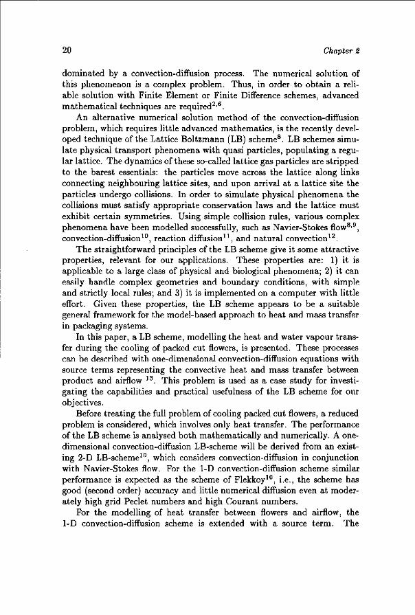
Figure 2.1: Comparison of the solution of LB scheme (symbols) with the exact solution (lines) of the problem of a semi-infinite packed bed with periodically varying heat source at the origin. Shown is the value of the wave vector K of the exact solution as a function of the Courant number U for the grid Peclet number Pe* = 1 and 100.

complex wave number K = kAx is computed using non-linear regression. These values have been compared with the root of Eq.(2.19), as is shown in figure 2.1.

For the range of Re(K) > —0.4 accurate results are obtained. The differences between the estimated and the exact values of K are within 2% for both Pe* = 1 and Pe* = 100. If the ratio of the macroscopic length scale k~l and the lattice spacing Ax approaches unity (fi «s K —¥ 1), the LB scheme looses accuracy, especially in the case of high Peclet numbers. This is not unexpected considering that the Chapman-Enskog expansion is valid only in the range of the Knudsen number fi < 1. As such, steep gradients can not be resolved accurately by the LB scheme. However, this is a property shared with many other numerical schemes.

3. Modelling the cooling of flowers

After checking the consistency of the LB scheme, an extended scheme for the problem of cooling cut flowers has been developed. Packed cut flow­ers are cooled by forcing cold air through the vent holes in the package and subsequently through the bed of flowers, as is shown in figure 2.2. In this case study, the packaging considered is in the middle of a large stack, with adjacent packages at all sides. All packages in the stack are ventilated with an equal amount of airflow. Consequently, the cooling process of flowers

26 Chapter 2

in the box in the middle of the stack can be treated as a one-dimensional problem. Further assumptions are: 1) The flower bed is a porous medium with homogeneous porosity, resulting in a uniform flow field through the bed. 2) The heat conduction of the solid phase of the flowerbed is negligible, due to limited contact between the individual flowers. 3) The heat production by respiration is negligible. 4) The flower plants maintain a saturated vapour pressure in their tissue. 5) The saturated vapour pressure is a function of the flower temperature. 6) There is vapour transfer between product and surrounding air, which is proportional to the vapour deficit between the plant tissue and the air.

':0 Oil

!:G o o o

Figure 2.2: Schematic diagram of packaging for cut flowers. The flowers face either side of the box and are wrapped in foil, indicated with dashed lines.

Applying the above assumptions the heat and vapour transfer can be described by the following equations2,5:

dtTa + udxTa = adlTa+sa(Tp-Ta),

dtTp = sp(Ta -Tp) + sw(ca -

dtca + udxca Dd2xca + sv(c°a

at-ca).

(2.21)

(2.22)

(2.23)

These equations are obtained by extending Eqs.(2.1)- (2.2) with a convection-diffusion equation governing the water vapour transport in air. The source term in Eq.(2.23) accounts for the evaporation of water from the cell tissue of the flowers. The heat of evaporation is extracted from the heat of the flowers and is accounted for by the extra source term in Eq.(2.21).

The relaxation constants:

aA spec aA spec

PaCPae ppCpA1-*) SfM

r0A PPcPp(l-e)

spec /U spec

(2.24)

Cooling of packed cut flowers 27

are determined by the heat and mass transfer coefficient of the flower plant tissue and the boundary layer between the flower and the surrounding air flow.

The description of the physical system, Eqs.(2.21)-(2.23), is completed with the initial and boundary conditions at the in-flow (x = 0) and out-flow (x = L) boundaries of the bed of product:

Ta=Tp=Tl,ca = csaat(Tl), for all x > 0, at t = 0; (2.25)

Ta = T0, ca = ca0, for all t, at x = 0, (2.26)

dxTa = dxca = 0, for all t, at x = L. (2.27)

The modelling of the vapour transfer during cooling requires that an­other lattice gas with distribution function v,- is introduced in the LB scheme. The density of this lattice gas represents the vapour density 52. Vj = pv. The particle distribution D,- evolves according to a LB equa­tion similar to Eq.(2.11). The density of the vapour particles in the flowers is maintained at the saturation vapour pressure ps

vat and therefore it is

not modelled explicitly. The complete extended LB scheme describing the cooling of flowers is given below:

hi(x + Axi,t +At)-hi(x,t) = n^{x,t) + ^{x,t), (2.28)

Vi{x + Axi,t + At)-Vi{x,t) = Slvi(x,t) + <l>vi{x,t), (2.29)

pq(x,t + At)-Pg{x,t) = &{x,t) + $w(x,t). (2.30)

The collision operator,

Slvi(x,t)=u>v[v?{x,t)-vi{x,t)], (2.31)

describes the transport of vapour in the air flow and the transfer operators

*v{(x,t) = w^v[p

svat{x,t)-pv{x,t)], (2.32)

^(x,t) = 4>w[Pv(x,t)-plat{x,t)l (2.33)

describe the vapour transport by evaporation from flowers to air. For the definition of the other operators, we refer to the previous section.

The relations between the parameters in the LB scheme and the physical parameters are given by:

D = *i-5^i- = S = - = S- (2'34)

28 Chapter 2

3.1. Initial and boundary conditions

The initial particle distributions are set equal to the equilibrium distri­butions corresponding with the initial temperature phi = 7\ and vapour concentration pv\ = cs

aat(Ti), i.e.,

hi{x,t = 0) = h?{ph0),

Vi{x,t = 0) = vlq{pv0),

pq(x,t = 0) = ph0.

(2.35)

(2.36)

(2.37)

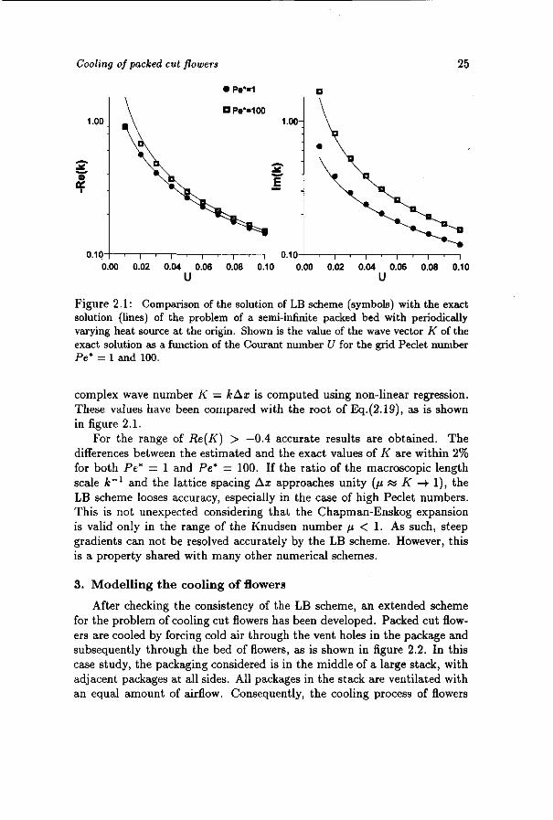
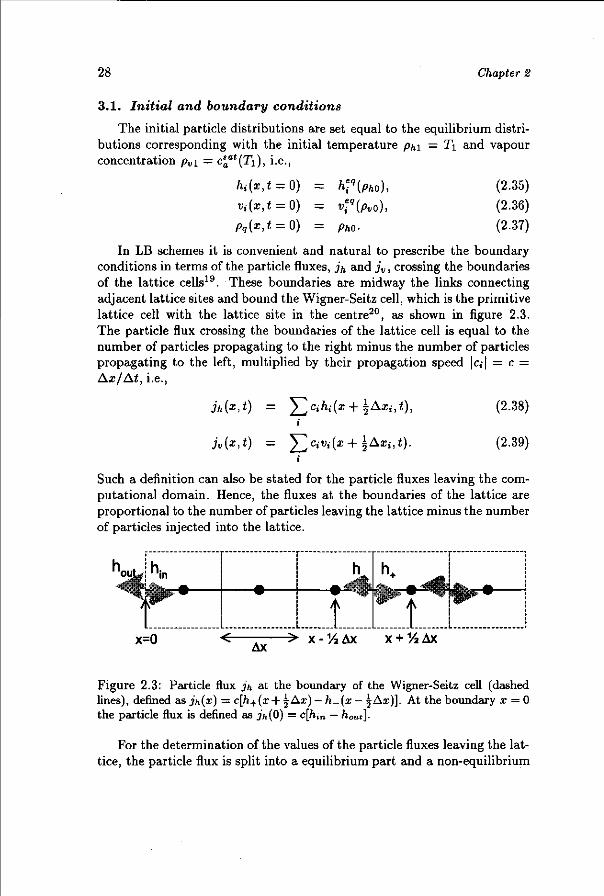
In LB schemes it is convenient and natural to prescribe the boundary conditions in terms of the particle fluxes, jh and j v , crossing the boundaries of the lattice cells19. These boundaries are midway the links connecting adjacent lattice sites and bound the Wigner-Seitz cell, which is the primitive lattice cell with the lattice site in the centre20, as shown in figure 2.3. The particle flux crossing the boundaries of the lattice cell is equal to the number of particles propagating to the right minus the number of particles propagating to the left, multiplied by their propagation speed |c,| = c = Ax/At, i.e.,

jh{x,t) = YlCih'(x + hAx''t)' i

jv(x,t) - ^2ciVi(x + ^Axi,t).

(2.38)

(2.39)

Such a definition can also be stated for the particle fluxes leaving the com­putational domain. Hence, the fluxes at the boundaries of the lattice are proportional to the number of particles leaving the lattice minus the number of particles injected into the lattice.

9 *«lf-!lk

1 x=0

Ax -> x-14Ax x + 1/2Ax

Figure 2.3: Particle flux jh at the boundary of the Wigner-Seitz cell (dashed lines), defined as jh{x) = c[h+(x + |Ax) — h-(x — ^Ax)]. At the boundary x = 0 the particle flux is defined as jh(0) = c[h,n — hout]-

For the determination of the values of the particle fluxes leaving the lat­tice, the particle flux is split into a equilibrium part and a non-equilibrium

Cooling of packed cut flowers 29

part: jh = jlq + j ^ e q . The equilibrium particle flux is due to the exter­nally applied velocity field: j ^ q = phu. The non-equilibrium particle flux is due to gradients in the number density and follows Fouriers law or Ficks law. For the computation of the non-equilibrium particle flux at the inlet a first order approximation of Fouriers law and Ficks law is used. At the outlet (x = L) the gradients are zero according to the boundary conditions Eq.(2.27). Hence, the boundary conditions, stated as prescription of the particle fluxes leaving the lattice, are given by:

jh{x = Q,t) = T^—[ph{x=^Ax,t)-phl] + phlu, (2.40) ±Ax

jv{x = Q,t) = Y—\Pv(x=\^-x>t)-Pvi\+Pviu> (2-41) 2 A.X

jh(x = L,t) = Ph(x = L--Ax,t)u, (2.42)

jv{x-L,t) = pv{x-L--Ax,t)u. (2.43)

Here, phi and pv\ are the densities of heat and water vapour particles at the inlet respectively.

As the boundaries of the computation domain coincide with the bound­aries of the lattice cells, they are displaced half a lattice spacing from the nearest lattice site. Therefore, the location of the lattice sites are labelled as x = ( | + n)Ax, with 0 < n < N — 1 and N = L/Ax the number of lattice sites.

3.2. Experiments

Simulation results, obtained by the LB scheme, are compared with data from cooling experiments performed with irises, cultivar Blue Magic. Irises are chosen since the flowerbed has a high degree of homogeneity in porosity and mass density. Due to the homogeneity of the porosity the airflow inside the flowerbed will be quite uniform.

The irises are packed in a commercially used box, made from corrugated board and measuring 1.20 m by 0.45 m by 0.30 m. The thickness of the corrugated board is 4 mm at the top and bottom, and 8 mm at the sides. At both ends of the box there are two vent holes (diameter = 6 cm). The flower buds face either ends of the box, as shown in figure 2.2. The box contains 18 bunches consisting of 50 irises each, having a total mass 35.5 kg. Each bunch is wrapped in polypropylene foil, which is impermeable to airflow and vapour transport. The foil wrapping is open at both ends of the bunch. As the bunch stacking in the box is very tight, it is assumed that the total flow is going through the bunches. The length of the flowerbed is

30 Chapter 2

1.00 m, leaving two headspaces of 0.10 m at both ends of the box.

ww/ww Figure 2.4: Experimental setup for monitoring the cooling of packaged flowers. On the left the container with four packagings is drawn. On the right the locations of the thermocouples are indicated.

The temperature of the flowers is monitored with copper-constantane thermocouples, which are inserted either in the back of the flower bud or the end of the stems. In total 20 thermocouples, more or less uniformly distributed over the front, middle and the back cross section, are used. The positions of these cross sections and the positions of the thermocouples within the cross section are indicated in figure 2.4.

The experiment is performed with cooling conditions as occur during road transport. Prior to the cooling, the packed flowers are stored for 24 hours in a climate room controlled at 19°C, giving the flowers a uniform initial temperature. After this pre-treatment the box with flowers is put in an insulated container. Also, 3 other identical boxes, which are filled with synthetic material (artificial lemons, partially filled with water), are placed in the container. The weight, and consequently, the heat capacity of the artificial lemons are about equal to that of the flowers. The airflow resistance of the artificial lemons is also comparable to that of the packed bed of irises. Due to the similarity in thermal and aerodynamic properties, and the low thermal conductivity of the corrugated board, it is assumed, that there is no heat flow from one box to another. Hence, the cooling of the packed irises is assumed to be a 1-D problem.

Cooling of packed cut flowers 31

Subsequently, the container with the boxes is stored in another climate room, which is controlled at a temperature of 3°C and a relative humidity of 90%. The temperature and the relative humidity of the air at the inlet are measured with a Vaisailla temperature and R.H.-sensor. With a fan system, the cold air from the room is forced into the container, flows through the boxes and exits again in the climate room. The container and the flow of air are indicated in figure 2.4. At the outlet the air flow velocity is measured with a hot wire anemometer. Due to the high turbulence and the division of the airflow over four boxes, the velocity field inside the box with flowers can not be obtained accurately. The fan system is regulated such that airflow velocity inside the flower box is in the range of 5-10 cm/s, which is the range of airflow inside packages during road transport.

The readings of the thermocouples and the Vaisalla sensor are recorded with a data logger, sampling at a 2 minutes interval. An average reading of the thermocouples over the last hour of the pre-treatment shows that the initial flower temperature is 18.8 ± 0.3°C. The inaccuracy in the initial flower temperature is mainly due to the non-uniformity of the temperature distribution. The average reading during cooling shows that the inlet air temperature is 2.8 ± 0.1°C and a relative humidity of 90 ± 5%.

The accuracy of the readings of the flower temperature during cooling is determined by averaging the values measured at the end of the cooling during which a steady state is obtained. Averaging 20 values of a single thermocouple shows a standard deviation of 0.014°C, and after averaging 20 readings from all thermocouples in the back cross section one obtains the average value of the final flower temperature of 2A°C with a standard deviation of 0.14°C. The low value of the standard deviation indicates a rather uniform temperature distribution in the back cross section. Other cross sections show similar standard deviations, and thereby substantiating the hypothesis that the cooling of the packed irises in this experiment is a 1-D phenomenon.

It is worth noting, that the final flower temperature, 2.4°C, is lower than the inlet air temperature, 2.8°C. This effect cannot be explained by an inaccuracy in the measurement of the temperatures. In fact, this difference is caused by the evaporation of water from the flower plant, which extracts heat from the flower and hence lowers the flower temperature below the air temperature13.

32

3.3. Simulation

Chapter 2

With the Lattice Boltzmann scheme the cooling of packed irises, as recorded in the previously described experiment, is simulated. The numer­ical results will be compared with the averaged flower temperatures in the three cross sections, which are indicated in figure 2.4.

20-

1 6 -

o o ~ 1 2 -<D

• Front cross section • Middle cross section • Back cross section

~i 1 1 1 r~ 120 240 360 480 600

Time (min) 720 840

Figure 2.5: Comparison of experiment (symbols) with simulation data from the LB scheme (lines). Shown is the change in time of the average flower temperature in three cross sections of the flower bed during cooling

The simulation with the LB scheme is performed with a lattice with 20 grid points and Courant number of U = uAt/Ax = 0.1, and a grid Peclet number Pe* ?« 250. In the case of U = 0.1, the error in the diffusion coefficient is less than 1%, see Eq.(A.lO).

The physical properties of the flowers are approximately equal to those of water 1. The initial flower temperature and the inlet air temperature and relative humidity are taken equal to the values measured during the exper­iment. Three remaining parameters, aAapec, flAspec and u, are difficult to determine, due to the intricate geometry of the individual flowers and the inaccuracy in the air velocity measurement. Thus, they are estimated from the experimental data by trial simulations.

Cooling of packed cut flowers 33

The yet undetermined parameters u, aAspec and f3Aspec, are adjusted, until the sum of squared residuals is minimised. In figure 2.5 the simulation results, computed with the final parameter set u=0.067 m/s, aAspec= 443 W/.m3.K and f3Aspec= 0.056 s _ 1 , can be seen.

Figure 2.5 shows that the simulation results correlate well with the experimental data. The simulation indeed shows that in the steady state at the end of cooling, the average flower temperature (in the middle and back cross section), Tp = 2A°C, is lower than the incoming air, To = 2.8°C. This phenomenon can indeed be explained by the extra cooling effect of the evaporation of water from the flowers.

4. Conclusions

For the analysis of the heat and mass transfer in packaging systems with cut flowers, a 1-D convection-diffusion Lattice Boltzmann scheme has been constructed. The consistency and accuracy of this scheme is checked by performing benchmark problems and by theoretical analysis.

In the first instance, a convection-diffusion scheme extended with source terms to represent the heat transfer from packed flowers to the airflow, is analysed. By means of the mathematical analysis of the Chapman-Enskog procedure and of numerical analysis, LB schemes have shown to accurately simulate the phenomena described with convection-diffusion and simulta­neous heat transfer, e.g., Eqs.(2.1)-(2.2). Accurate agreement with exact solutions is found for both low and high grid Peclet numbers Pe*, with the restriction that the gradient should not be too steep. Since large gradients in temperature or vapour density in systems of packed agricultural prod­ucts seldom occur in practice, the limitation of the LB scheme is not very restrictive for our applications.

Finally, the extended LB scheme is applied to the problem of cooling packaged cut flowers. Next to heat flow phenomena, the scheme also de­scribes the vapour flow phenomena. The scheme is able to simulate cooling experiments with packed irises with reasonable accuracy. The simulation is performed with high grid Peclet numbers, i.e. Pe* fa 250 and with a small amount of resources (lattice of 20 grid points).

Based on the results of this study, it is concluded that the Lattice Boltz­mann scheme is suitable as a generic modelling technique for the simulation of physical processes in packages of agricultural products. In future research the scheme will be extended to higher dimensions and with other physical phenomena, such as natural convection.

34 Chapter 2

Appendix A Chapman Enskog procedure

The application of the Chapman-Enskog procedure to a Lattice Boltz-mann Equation reveals its macroscopic behaviour, as triggered by small departures of the equilibrium distribution8.

In the Chapman-Enskog expansion the particle distribution function /i,-is expanded as a power series of the Knudsen number fi, which is the ratio of the mean free path and the macroscopic length scale: fi ~ Axdxph/ Ph-The expansion of hi around its equilibrium distribution is:

hi = h? + fih^ + fi2h\2) + ... (A.l)

It must be noted that the Chapman-Enskog expansion is made under the assumption that ft < I.

Also space and time derivatives of hi are expanded as series in powers of ft. The Chapman-Enskog procedure introduces two time scales, a fast time scale, t\, associated with convective (inertial) processes and a slow time scale, <2i associated with dissipative processes, i.e. heat conduction. By the introduction of the two time scales into the time derivative and the substitution x\ — fix/Ax in the spatial derivative the following is obtained:

Axdxhi = fidXlhi (A.2)

Atdthi = fidtlhi + fi2dt2hi (A.3)

As the heat transfer process, modelled by $^, is also a dissipative process it can be assumed that it also scales as p.2: <£̂ = Wifi2(f>h(ph — Pq) •

After substitution of the expansions Eqs.(A.l)- (A.3) into the LB scheme, Eqs.(2.11)-(2.14), performing a Taylor expansion of hi(x + Axi,t + At), and collecting terms of equal order in fi, one obtains the following hierarchy of equations:

-UhhV = (dtl + eidXl)h? (A.4)

-Wh/42) = {dtl+eidXifhT + {dtl+eidXl)h^+dt2h^ (A.5)

Here, e,- = C{At/Ax.

After summing Eq.(A.4) over all states and using ^ t - h\n> = 0, one obtains the evolution of the density ph for short time scales, with U = uAt/Ax the Courant number:

dtlPh + Udtlph = 0. (A.6)

Observe, that at short time scales the density evolves according to the continuity equation, as must be expected.

Cooling of packed cut flowers 35

Substitution of Eq.(A.4) in Eq.(A.5) and summat ion over all s tates, gives the contribution of the long t ime scale to the evolution of ph '•

dt2Pk = ( — - b(l - U2)d2XiPh + 4>h{pq ~ Ph) (A.7)

The PDE describing the evolution of pq follows directly from the expan­sion of Eq(2.14). The complete set of PDE's , Eqs.(2.1)- (2.2), is recovered when the contributions of both t imes scales ,t\ and <2, are added:

dtph + udxph = Dhdlph + —(pq- ph) (A.8)

dtPq = ^(Ph-pq) (A.9)

For the diffusion coefficient, it follows that :

The velocity dependent term (1 — U2) is a consequence of the lack of Galilean-invariance of the Lattice Boltzmann scheme, presented in this pa­per.

The velocity dependence is negligible in the limit of low Courant num­bers U. However, recently it is shown, tha t the velocity dependent term can be eliminated, if rest particles with c,- = 0 are introduced and if quadratic terms in U are incorporated in the equilibrium distr ibution2 2 .

G. van Beek and H.F.Th. Meffert, Cooling of horticultural product with heat and mass transfer by diffusion. In Developments in Food Preservation, Vol.1 (Edited by E. Thome), 39-92, Applied Science Publishers, London (1981). K.J. Beukema, Heat and mass transfer during cooling and storage of agricul­tural products as influenced by natural convection, Ph. D. Thesis, Agricul­tural University, Wageningen, the Netherlands (1980). R.G.M. van der Sman, R.G. Evelo, E.C. Wilkinson and W.G. van Doom, Quality loss in packed rose flowers due to Botrytis cinerea as related to tem­perature regimes and packaging design, Postharvest Biol, and Techn. 7, 341-350 (1996). C.D. Baird and J.J. Gaffney, A numerical procedure for calculating heat transfer in bulk loads of fruits or vegetables, Trans. ASHRAE 82 (2), 525-540 (1982).

36 Chapter 2

5. F.W. Bakker-Arkema, W.G. Bickert and R.J. Patterson, Simultaneous Heat and Mass Transfer during the Cooling of a Deep Bed of Biological Products under Varying Inlet Air Conditions, J. Agr. Eng. Research 12 (4), 297-307 (1967).

6. K.K. Khankari, S.V. Patankar and R.V. Morey, A mathematical model for natural convection moisture migration in stored grain, ASEA-paper 93-6017, 1-29 (1993).

7. G. Comini, G. Cortella and O. Saro, Finite element analysis of coupled con­duction and convection in refrigerated transport, Int. J. Refrig. 18 (2), 123-131 (1995).

8. U. Frisch, D. d'Humieres D., B. Hasslacher, Y. Pomeau and Rivet J.P., Lattice Gas Hydrodynamics in Two and Three Dimensions, Complex Systems 1, 649-707 (1987).

9. J.M.V.A. Koelman, A Simple Lattice Boltzmann Scheme for Navier-Stokes Fluid Flow, Europhys. Lett., 15 (6), 603-607 (1991).

10. E.G. Flekkoy, Lattice BGK Model for Miscible Fluids, Phys. Rev. E 47 , 4247- (1993).

11. S. Ponce-Dawson, S. Chen, and G.D. Doolen, Lattice Boltzmann computa­tions for reaction-diffusion equations, J. Chem. Phys. 9 8 (2), 1514-1523 (1993).

12. J.G.M. Eggels and J. A. Somers, Numerical simulation of free convective flow using the lattice-Boltzmann scheme, Int. J. Heat and Fluid Flow, 1 5 , 357-364, (1995).

13. H. Wang, C. Ceton, and S. Touber, Modelling the micro-climate of packed cut flowers during pre-cooling. Proc. 19th Int. Congress of Refrigeration, the Hague, Netherlands, 707-714, (1995).

14. R. Benzi R., Succi S., and Vergassola.M. The lattice Boltzmann equation: theory and applications. Phys. Rep., 222(3): 145-197, (1992).

15. P. Bhatnagar, E.P. Gross and M.K. Krook, Phys. Rev. 94 , 511, (1954). 16. S. Chapman and T.G. Cowling, The Mathematical Theory of Non-Uniform

gasses. Cambridge Univ. Press, Cambridge (1939). 17. Y.H. Qian, D. d'Humieres and P. Lallemand, Lattice BGK Models for Navier-

Stokes Equation, Europhys.Lett., 17 (6), 479-484 (1992). 18. FIDAP v7.0, Fluid Dynamics International, Evanston, 111., USA, (1993). 19. J.A. Somers and P.C. Rem, Flow computation with lattice gasses, Appl. Sci.

Research, 48 (3-4), 391-436, (1991). 20. C. Kittel, Introduction to Solid State Physics, John Wiley & Sons, N.Y.

(1953). 21. S.V. Patankar, Numerical Heat Transfer and Fluid Flow, Hemisphere Publ.,

N.Y. (1980). 22. M.R. Swift, E. Orlandini, W.R. Osborn, J.M. Yeomans, Lattice Boltzmann

Simulations of Liquid Gas and Binary Fluid Systems, Phys. Rev. E, 5 4 (5), 5041-5052, (1996).

Chapter 3

Natural convection in potato containers

1. Introduction

Due to their simple nature Lattice Boltzmann schemes are very suitable for modelling the strongly coupled heat and mass transfer phenomena occur­ring in packaging systems for agricultural products1. LB schemes2 are a special class of lattice gas automata3 (LGA), which can reproduce various complex physical phenomena as hydrodynamics4, natural convection5, and reaction-diffusion6. The basic idea behind LGA is to model physical phe­nomena with quasi-particles, representing packets of matter or fluid. The quasi-particles move over a discrete regular lattice and collide according to simple rules.

In this paper a Lattice Boltzmann scheme is presented, which models the natural convection in a porous medium with internal heat generation. This scheme is applied to the problem of heat transfer in a 1000 kg corrugated board container for seed potatoes. Before approaching the practical prob­lem, model problems with known analytical solutions are addressed. The LB scheme is tested by comparing the computed results with the analytical solutions. Then, the LB scheme is used to simulate the cooling behaviour of potato containers. The results of the LB scheme are compared with the experimental data.

Heat transfer between the packaged potatoes and their environment is caused by two processes: 1) convection of heat by air flow in voids be-

appeared as: R.G.M. van der Sman, Lattice Boltzmann scheme for natural convec­tion in porous media. Int. J. Modern Phys. C 8(4): 879-888 (1997).

37

38 Chapter 3

tween potatoes, and 2) heat conduction through the potatoes, air and the corrugated board packaging material. As is usual in the field of agricul­tural engineering the potatoes are treated as a single phase porous medium, which enables heat transfer by both conduction and convection7,8,9. The air flow is driven by natural convection, which is due to temperature differ­ences between the potatoes and the environment. The respiration process of the potatoes generate a large amount of heat, and therefore contribute significantly to the temperature difference between the potatoes and the environment.

In the single phase approximation the evolution of the temperature T is decribed by a convection diffusion equation with an extra source term for the internal heat generation (Q)8,9:

PPcPpdtT + PacPaxi-VT = ApV2T + Q. (3.1)

Here pacPa is the heat capacity of air, ppcPp the heat capacity of the porous medium, and Ap the heat conductivity of the porous medium. The air velocity field u is described by the continuity equation and a modified Darcy's law8,9:

V -p„u = 0, (3.2)

- V p - - p a u + g p o ( l - / ? ( T - T o ) ) = 0. (3.3) K

The modified Darcy's law has an extra term modelling the buoyancy force, for which the Boussinesq approximation is applied. In Eq.(3.3) v is the kinematic viscosity, K the permeability of the porous medium, and /? the thermal expansion coefficient. The reference density po and temperature To are taken equal to the ambient air density and temperature.

After substitution of Darcy's law in the continuity equation, one obtains a Poisson equation for the pressure, with a source term proportional to the temperature gradient. The resulting pressure field will be independent of the permeability of the porous medium K, although the permeability does determine the flow rate, as stated in Darcy's law.

The description of natural convection in potato containers is completed with the statement of the boundary conditions, describing the imperme­ability of the packaging material to air flow

dnP = 0, (3.4)

and the heat conduction through the cardboard walls:

\pdnT=-^(T-T0). (3.5)

Natural convection in potato containers 39

Here is Ac the thermal conductivity of the packaging material and dc the thickness of the packaging material.

2. Lattice Boltzmann scheme

For the numerical simulation of natural convection in porous media, a Lat­tice Boltzmann scheme with two lattice gasses <?,• and /,•, modelling the heat transport and the fluid flow respectively, is used. These lattice gasses reside on a three-dimensional six-velocity lattice with two-fold symmetry, which is sufficient for processes involving conservation of mass only3. The lattice, used in the simulation, is drawn in figure 3.1.

The particle distribution functions qt(x,t) and fi(x,t) represent the number of lattice particles at lattice site x at time t propagating with ve­locity c,- = Ax,-/Ai. The particle number densities, i.e. heat energy density and mass density, are related to the macroscopic variables temperature and pressure, in the following way:

Pq = £ > = T, (3.6) i

Pf - ]C & = P"~P- (3J) i

The Lattice Boltzmann scheme for the heat transport is equal to the convection diffusion scheme10 with an extra source term u>iQ/ppcPp = Wi£, representing the internal heat generation:

^ ( x + A x ^ + At) = g i (x , i )+wjg je 9 (x ,<)-9i (x , i ) ] + ^ , (3.8)

„?« = Wi[pq + C-Hlfl]. (3.9)

The velocity field uq is defined as:

_ PaCpa (3.10) PpcpP

This scheme is a so-called Lattice BGK-scheme, of which the collision rules are derived from the discretization of the BGK approximation of the Boltz­mann equation11. The collision rules of this scheme describe a relaxation process towards an equilibrium distribution q^q with a single parameter ujq. The relaxation parameter toq is related to the heat diffusion coefficient a:

The parameter cs is the so-called speed of sound of the lattice gas, which is a property of the lattice with its associated set of particle velocities {c,}.

40 Chapter 3

The convection field acts on the lattice gas as a displacement of the equilibrium distribution with an amount proportional to the equilibrium heat flux j q

g = pquq. In absence of the velocity field uq the equilibrium dis­tribution is equal to the distribution for pure diffusion, which is a weighted function of the density pq.

The phenomena described by the convection diffusion equation and the modified Darcy's law are both a result of 1) a diffusive process and 2) an externally applied field. Using this similarity, a Lattice BGK scheme for the fluid dynamics is constructed. The equilibrium distribution f?q is displaced by an amount proportional to the equilibrium mass flux flux jy9, which follows from Darcy's law after setting Vp = 0. The LB scheme for the fluid dynamics is then:

/,(x + Ax,-,s + AS) = / , (x,s)+w / [ / ;9(x,S)- / i(x,s)] , (3.12)

• eg

f!" = ^[Pf + ^ - l (3.13)

?f = -%0g[l-p{pq-pl)]ez. (3.14)

The fluid dynamics LB scheme actually solves the Poisson equation for the pressure field as a relaxation scheme, so instead of the time variable t, the counter s is used. The relaxation parameter can now be set to an arbitrary value. Setting uif = 1 is the most optimal choice with respect to computing time. The stationary state of the fluid dynamics LB scheme will give a second order approximation of the solution of Eqs.(3.2)-(3.3), which can be proven by performing the Chapman-Enskog expansion3,10 of the LB equation.

Next to the pressure field, also the velocity field follows immediately from our LB scheme. It should be noted that the usual computation of the velocity field from the particle distribution at a lattice site, pju = ^ t - c,/,-, as done in hydrodynamic LB schemes, is not correct for our scheme. This is due to the fact that momentum is not conserved during collisions. The velocity field must be determined from the mass fluxes jf, which are only defined on the boundaries of the Wigner-Seitz cells of the lattice, which are midway the lattice sites12. The definition of these mass fluxes follows easily from figure 3.1:

j / ( x + -Ax,-,*) = Cifi(x+ Axi,t) + Cjfj(x,t) , with c,- = - c , . (3.15)

The flow velocity at a lattice site can now be calculated by averaging the mass fluxes on the boundaries of its Wigner-Seitz cell:

/ ) /u(x,«) = ^ c i [ / i ( x + Ax i ,<) + /1(x, i )] . (3.16)

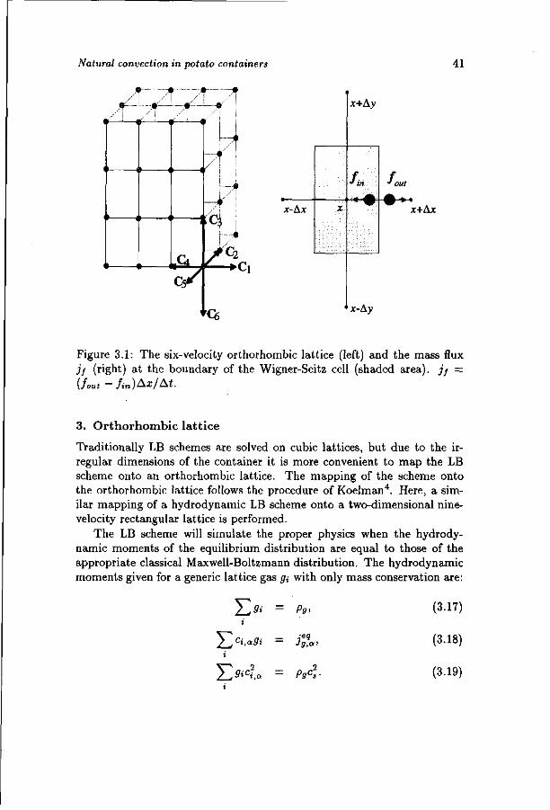
Natural convection in potato containers 41

< p~

f~—'—'

<> 1

* -;i

ff-f ! «

1 (

I - ' »

-jf- L

h—'' 9

1 !

c 5 ^

<

— • ; »

•

-—p

Qj

x-Ax

x+Ay

f * in

x+Ax

x-Ay

Figure 3.1: The six-velocity orthorhombic lattice (left) and the mass flux jf (right) at the boundary of the Wigner-Seitz cell (shaded area), jj = {font - fin) Ax/At.

3. O r thorhombic la t t ice

Traditionally LB schemes are solved on cubic lattices, but due to the ir­regular dimensions of the container it is more convenient to map the LB scheme onto an orthorhombic lattice. The mapping of the scheme onto the orthorhombic lattice follows the procedure of Koelman4. Here, a sim­ilar mapping of a hydrodynamic LB scheme onto a two-dimensional nine-velocity rectangular lattice is performed.

The LB scheme will simulate the proper physics when the hydrody­namic moments of the equilibrium distribution are equal to those of the appropriate classical Maxwell-Boltzmann distribution. The hydrodynamic moments given for a generic lattice gas <?,- with only mass conservation are:

5Z«< 2J ci,*9i

Ys9iCl°

= Pg,

_ jeq

= Pgcl

(3.17)

(3.18)

(3.19)

42 Chapter 3

The equilibrium distributions in Eq.(3.9) and Eq.(3.13) satisfies the above stated constraints. The formula for the equilibrium distribution q^q is equal to the one of the convection diffusion LB scheme10, which is mapped onto a square lattice. So the difference in geometry of the lattice is only apparent in the different values for the weight factors Wj and the speed of sound cs. The weight factors and the speed of sound are given by:

,._iL.I_yJ_ 2c2 (3.20)

4. Boundary Conditions

The mapping of the lattice is done such that the boundaries of the Wigner Seitz cells of the exterior lattice sites coincide with the walls of the box, as shown in figure 3.2. Because of the symmetry of the container, the computation domain consists of a quarter of the total packaging system.

packaging material

00

ft.

symmetry line

Figure 3.2: Mapping of the octagonal container on the orthorhombic lattice. Shown is the horizontal cross section. The boundaries of the calculation domain are not coincident with lattice sites (dots), but with the boundaries of the Wigner Seitz cells (dashed lines).

The boundary conditions at the walls of the container are formulated in terms of mass and heat fluxes, crossing the boundaries of the Wigner

Natural convection in potato containers 43

Seitz cells. As stated in Eq.(3.15) the mass and heat flux crossing these boundaries are proportional to the number of particles ejected from the porous medium minus the number of particles injected into the porous medium. The difference between ejected and injected heat and momentum particles can be derived from the boundary conditions Eqs.(3.4)-(3.5). The heat and mass fluxes through cardboard walls parallel to one of the lattice principal directions en are giving by

1 jg(x) = 4>q0t\pq(x - 2 A x » ) - A#en,

J/W = o, 1 1 1

^ p " ~~ ~^ cj)eqxt'

J.int _ a lext _^c 1 *q ~ iAr ' Pq ~ d D C '

(3.21)

(3.22)

(3.23)

(3.24)

The heat flux is stated as a quotient of a temperature difference and the heat resistance between the most exterior lattice site and the ambient, which is equal to the heat resistance of a half Wigner-Seitz cell in series with the heat resistance of the packaging material. As the packaging material is impermeable to air flow, the mass flux is zero.

The skew vertical cardboard wall is not parallel to a principal direction of the lattice, as shown in figure 3.2. In this case there are two heat fluxes from one exterior lattice site: jq>x = cx{qout - g , „ ) and jqiV = cy(qout -qin)• These fluxes are also expressed as a quotient of a temperature difference and a heat resistance:

j , , a (x ) = ^ > g ( x - A x a ) - p ° ] e a , (3.25)

1 ' +i> (3-26) Xtot Amt A. <?>'

lint ^q,a

a Axa

(3.27)

^ = c o s ^ ^ 7 ^ ' ^ = s i n ( c ) Z 7 ^ ' (3'28)

"c Hpcpp " c fJpcpp

where the angle C is defined in figure 3.2

5. Analytical solutions

The correctness of our LB schemes is investigated by comparison with ana­lytical solutions of two simple 1-dimensional natural convection problems. The simulations are performed on the 3-D orthorhombic lattice. The ver­tical walls are assumed to be thermally insulating, and impervious to air

44 Chapter 3

flow. For the two problems considered, the top and bottom of the container are open. Here, constant ambient pressure and temperature are applied as boundary conditions. The pressure drop over the container is assumed to be purely due to gravity: p(Lz) — p(0) = pogLz.

As a first problem, the pressure and flow field for a constant non-uniform temperature field are calculated:

T(z) = Ti f o r 0 < 2 < ^Lz,

T(z) = T0fot^Lz<z<Lz.

From Darcy's law immediately follows the analytical solution, which states that there is a uniform velocity field, proportional with the average tem­perature T, and two regions with a linear pressure profile:

Pan = ^PogpTez, (3.29)

Vp = Pog[l - fip! - T] for 0 < z < ^Lz ,

Vp = Pog[l - 0(TO - T)] for \LZ<Z<LZ. (3.30)

The second problem addressed, is the temperature field generated by the heat production of the porous medium. With Maple™ the analytical solution of the velocity and temperature field for the stationary state of this problem, are obtained. The analytical solution of the pressure field is not known.

pau = -p0g/3Tez, (3.31)

T{z) = r o + i £ _ ^ 1 - e x p K ; / ; ) 0.32) uq uq l — exp{uqLz/a)

The results of the simulations are shown in figure 3.3. As one can see the simulations results are in good agreement with the analytical solutions for a wide range of parameters. The velocity fields, calculated with Eq.(3.16), are also in agreement with the analytical solution.

6. Exper iments

After testing the LB scheme against analytical solutions, it is applied to the problem of natural convection in seed potatoes containers. For the investigation of this problem cooling experiments are performed with two containers with different thicknesses of the sidewalls (17 mm and 40 mm).

Natural convection in potato containers 45

Height (m) Height (m)

Figure 3.3: Comparison of simulation data (solid lines) with analytical so­lutions (symbols) for two simple natural convection problems. Calculations are done for a range of the parameters Bo = /?(Ti with £ = 1.

• To) and Pe = uqLz/a,

The packaging designs are without vent holes. The octagonal corrugated cardboard container has a height of 1.60 m, and it is placed on pallets measuring 1.20 m by 1.00 m. The container is loaded with 1000 kg of seed potatoes. During the experiment the packed potatoes, with an initial tem­perature of about 12°C, are placed in a cold storage with an temperature of-3°C. At several locations along the central axis the potato temperature is measured for a period of 8 days.

The LB simulations are performed on a 16 x 6 x 6 lattice. The simu­lation results consist of the temperature fields and velocity fields at given time intervals. From these results the temperature profile along the central axis is extracted. The profile is plotted at a 2 day interval, and compared with experimental data. The values of most physical parameters describ­ing the natural convection process, see Eq.(3.1)-(3.3), are known from the literature8: pa, cPa, j3 and v are equal to the values for air; the bulk density of the potato load'*/9p=726 kg/m3; cPp =3.637 kJ/kg/K, Ap = 0.30 W/m/K, Ac = 44 mW/m/K, Q=7 W/m3 .

The permeability of the porous medium, K, can be roughly estimated by measuring the air flow resistance of a packed bed of potatoes at relatively high air velocities. The permeability is fine-tuned towards the value K — 2461 m2, in order to have a good fit between the numerical results and the

46 Chapter 3

Wall Thickness =17 mm Wall Thickness = 40 mm

i — i 1 i 1 1 r 0 0.2 0.4 0.6 0.8 1.0 1.2 1.4 1

i 1 1 1 1 r 0 0.2 0.4 0.6 0.8 1.0 1.2 1.4 1.6

Height (m) Height (m)

Figure 3.4: Comparison of simulation data (lines) with experimental data obtained from cooling experiments with two types of containers with 17mm and 40mm thick cardboard walls. Shown are the temperature profiles along the central axis at a two day interval. The initial temperature distribution is non-uniform (dashed line).

experimental data, obtained for the container with 17 mm thickness. Next, the simulation is performed for the other container with 40 mm thickness, using K = 2461 m2. The final results are shown in figure 3.4, from which can be concluded that for both packaging designs the experimental and simulation data are in good agreement.

7. Conclusions

A Lattice Boltzmann scheme is developed, which is able to model the heat transfer by natural convection and conduction in porous media. The scheme has been checked against two problems with analytical solutions. Next, cooling experiments performed with potato containers are simulated. Good agreement between experimental data and numerical results is found.

The (convection-diffusion) LB scheme is mapped on an orthorhombic lattice. To our knowledge this has not been done before. Computational domains with irregular dimensions are more easily mapped on orthorombic lattices than on cubic lattices. The use of orthorhombic lattices can result in the reduction of the number of sites on the lattice and computation time

Natural convection in potato containers 47

compared to cubic lattices. Boundary conditions are formulated using an uniform paradigm, based

on the particle fluxes crossing the boundaries of the Wigner Sites cells. This new formalism shows opportunities for using in fluid flow problems, where a consistent formalism is still not present1 3 , 1 4 .

1. R.G.M. van der Sman, and M.H. Ernst, Int. J. of Heat and Mass Transfer, submitted (1998); Chapter 2

2. R. Benzi R., Succi S., and Vergassola,M. The lattice Boltzmann equation: theory and applications. Phys. Rep., 222(3): 145-197, (1992).

3. U. Frisch, et.al., Lattice Gas Hydrodynamics in Two and Three Dimensions, Complex Systems 1, 649-707 (1987). See also, Lattice gas methods for partial differential equations, G.D. Doolen (ed), Addison-Wesley Publ. Co., p.75, (1989).

4. J.M.V.A. Koelman, A Simple Lattice Boltzmann Scheme for Navier-Stokes Fluid Flow, Europhys. Lett., 15 (6), 603-607 (1991).

5. J.G.M. Eggels and J. A. Somers, Numerical simulation of free convective flow using the lattice-Boltzmann scheme, Int. J. Heat and Fluid Flow 16, 357-364 (1995).

6. S. Ponce-Dawson, S. Chen, and G.D. Doolen, Lattice Boltzmann computa­tions for reaction-diffusion equations, J. Chem. Phys. 9 8 (2), 1514-1523 (1993).

7. F.W. Bakker-Arkema, W.G. Bickert and R.J. Patterson, Simultaneous Heat and Mass Transfer during the Cooling of a Deep Bed of Biological Products under Varying Inlet Air Conditions, J. Agr. Eng. Research 12 (4), 297-307 (1967).

8. K.J. Beukema, Heat and mass transfer during cooling and storage of agri­cultural products as influenced by natural convection, Ph. D. Thesis, Agr. Univ., Wageningen, the Netherlands (1980).

9. K.K. Khankari, S.V. Patankar and R.V. Morey, A mathematical model for natural convection moisture migration in stored grain, ASEA-paper 93-6017, 1-29 (1993).

10. E.G. Flekkoy, Lattice BGK Model for Miscible Fluids, Phys. Rev. E 47 , 4247- (1993).

11. P. Bhatnagar, E.P. Gross and M.K. Krook, Phys. Rev. 94 , 511, (1954). 12. G.R. McNamara, Europhys. Lett. 12, 329 (1990). 13. D.R. Noble et.al., A consistent hydrodynamic boundary condition for the

lattice Boltzmann method. Phys. Fluids 7, 203 (1995). 14. I. Ginzbourg, and D.d'Humieres, Local second-order boundary method for

Lattice Boltzmann models. J. Stat. Phys., 84 (5-6), 927 (1996).

Chapter 4

The vent hole design problem of a po ta to container

1. Introduction

In packaging systems of agricultural products the control of heat and mass transfer is of great importance for maintaining the quality of the packed product. The package must prevent the accumulation of heat and the condensation of moisture, which leads to degradation of quality. On the other hand, the package must protect the packed product from dehydration and adverse outside temperatures, which also affects the product quality. For every type of product, there are certain limits for the heat and mass transfer to the environment.

A convenient and frequently used means for controlling the heat and mass transfer in packages consists of vent holes. However, little fundamental knowledge or guidelines are available for an effective design of the vent holes. Using a numerical model, describing the heat and mass transfer in detail, this knowledge can be acquired and be used in designing vent holes.

In this paper, the problem of designing vent holes for containers of seed potatoes is studied. These containers, known as octabins, are made of cor­rugated board, hold 1000 kg of seed potatoes and have an octagonal shape.

to appear as: R.G.M. van der Sman, Solving the vent hole design problem for seed potato packagings with the Lattice Boltzmann scheme. Int. J. Comp. Fluid Dyn. (1998).

49

50 Chapter J,

They are used during road transport and storage prior to planting. During road transport, which occurs in winter time, there is a risk of moisture condensation on the potatoes, because the outside temperatures can be significantly colder than the initial potato temperature of 8°C.

By means of a numerical model, we search a vent hole design of the seed potato container, that avoids condensation during the cooling conditions of road transport. The numerical model is an extension of the Lattice Boltzmann scheme 1, which is used for modelling the natural convection inside a seed potato container without vent holes.

The Lattice Boltzmann (LB) scheme is a technique recently developed for modelling complex physical transport phenomena2, such as hydrody­namics, natural convection and multi-phase flow3,4,5, and the strongly cou­pled heat and mass transfer phenomena, which occur in packaging systems of agricultural products6,7.

LB schemes take a particle description of matter, using so-called lattice gas particles. These particles carry macroscopic portions of physical quan­tities, such as mass, momentum, and energy. The lattice gas particles exist on a regular lattice. During each timestep, the lattice gas particles jump to neighbouring lattice sites, and subsequently, they scatter according to simple collision rules. These collision rules satisfy appropriate conserva­tion laws. Despite their crude approximation of particle dynamics at the molecular level, LB schemes have shown to obey - to a good approxima­tion - the desired continuum equations. Consequently, they can be used for studying phenomena at macroscopic time and length scales. Nevertheless, they retain the advantages of a particle description, including clear physical insight and easy implementation of boundary conditions.

The properties, mentioned above, make LB schemes very suitable as a generic framework for modelling the phenomena in packaging systems6,7. This study is the first one, that applies the LB scheme to solve a design problem for a packaging system, which is actually going to be used in prac­tice. Therefore, the vent hole design of the seed potato container represents the ultimate test case for the use of LB schemes as a modelling framework for heat and mass transfer in packaging systems for agricultural products.

2. Problem Description

During cooling, the heat and mass transfer in the seed potato container involves a variety of processes: 1) convection of heat and water vapour by airflow in the voids between the packed products; 2) heat conduction through the products, air and packaging material; 3) water vapour diffusion through the packaging material; 4) evaporation of water from the product; 5) condensation of water vapour on the product, and 6) the ventilation of

The vent hole design problem of a potato container 51

heat and water vapour through the vent holes in the container. For the description of these processes, the usual assumption, that packed

agricultural products can be represented as a porous medium8,9,10, is taken. In the regime of natural convection, the air temperature can be taken equal to the product temperature. Hence, the heat transfer can be described with a single energy equation. This equation has contributions from the heat conduction of packed product, and the convection of heat by the airflow.

The porous medium also allows water vapour transfer, which is due to the airflow and evaporation and condensation. Hence, the time evolution of the concentration ca of water vapour in air is described by a convection diffusion equation with several source terms9:

dtca +u-Vca = DV2ca + Sap + Sam. (4.1)

Here, u is the velocity field, D is the diffusivity of water vapour in air. Sap

and Sam are source terms, representing the evaporation and condensation. These source terms are also part of the mass balances of the water content in the potatoes pw and of the amount of condensed moisture pm:

dtPw = -Sap (4.2)

dtpm = -Sam (4.3)

Both source terms are proportional with the difference between the wa­ter vapour concentration in air ca and the saturated water vapour con­centration c'a

at, which is maintained in the boundary layers above the skin of the potatoes and above the condensed moisture. The saturated water vapour concentration cs

aat is a function of the potato temperature

Caat=Ca

at(Tp). However, evaporation and condensation can not occur simultaneously.

Therefore, three regimes of mass transfer have to be differentiated:

a) Evaporation of water from the potato tissue, if ca < csaat and pm = 0,

b) Condensation of moisture, if ca > csaat, and

c) Evaporation of condensed moisture, if ca < csaat and pm > 0.

The condensed moisture is deposited on the potato. If the skin of the potato is covered with moisture, the evaporation of water from the potato is blocked. For clarity we have depicted the three ways of convective mass transfer occurring in the potato package of figure 4.1.

52 Chapter 4

The rates of the convective mass transfer are given by:

Sap = /3apAspec(csaat - ca) if pm=0, and (4.4)

0, otherwise.

Sam = PamAspec(csaat - ca) \ipm >0 or ca > c'a

at, and (4.5)

0, otherwise.

Here, Aspec is the specific area of the packed product, and /Jap and /?am are mass transfer coefficients.

Ca < C,sat CQ > CQsat C, < Ca

sat

a a 3 9 a a

Pm = 0 Pm > 0 Pm > 0

Figure 4.1: Convective mass transfer processes occurring in seed potato contain­ers: a) Evaporation of water from the potato, b) Condensation, and c) Evapo­ration of condensed moisture. In cases b) and c) there is a film of condensed moisture on the potatoes.

The energy equation is also a convection diffusion equation with extra source terms9:

PPcPpdtT + PacPau • VT = APV2T +Q + rSap + rSam. (4.6)

Here, Ap is the heat conduction of the porous medium, Q the heat of respira­tion, r the latent heat of water, ppcPp and pacPa the specific heat capacities of respectively the packed product and the air.

The velocity field, u, of the airflow is driven by natural convection. It is described by Darcy's law (extended with a Boussinesq term) and the continuity equation:

- V p - - / > 0 u + g p o ( l - / ? ( T - : T o ) ) = 0 (4.7) K

V-Pau = 0 (4.8)

The vent hole design problem of a potato container 53

Here, p is the pressure, u the viscosity of air, « the permeability of the porous medium, pa the mass density of air, g the gravitational acceleration, /? the isothermal expansion coefficient, To the ambient temperature and po the mass density of the ambient air.

The problem description, Eq.(4.1)-(4.8), is completed with the state­ment of the boundary conditions. The walls of the container are imperme­able to airflow, but allow heat conduction and mass transfer by diffusion. These boundary conditions are expressed as:

dnp = 0 ; - XpdnT = ^(T -T0); - Ddnca = ^(ca - c„). (4.9) ac dc

Here, Ac is the heat conductivity of the container wall, Dc is the water vapour diffusivity of the container wall, dc is the thickness of the container wall, Co is the water vapour density of the ambient air, and dn the spatial derivative normal to the wall surface.

Vent holes can be cut out of the sidewalls, the lid and the bottom. They allow air exchange between the container and the environment. For vent holes, with inward flow, we assume ambient conditions:

P = Po ~ PogzZ ; T = T0 ; ca = c0, (4.10)

and for holes, with outward flow, free flow conditions:

P = Po - PogzZ ; dnT = 0 ; dnca = 0. (4.11)

3. Lattice Boltzmann schemes

The Lattice Boltzmann scheme gives a prescription for the evolution of the distribution function of the lattice gas particles, <7,(x,t). This function states the (ensemble averaged) number of particles at lattice site x and time t, moving along the lattice vector e,, which connects site x with site x+Ax,-. By their restriction to discrete values of space and time, the velocities of lattice gas particles form a discrete set: c; = Axj/Ai, as is shown is figure 4.2a. The macroscopic-observable physical quantities, which are carried by the lattice gas particles, are obtained by computing the moments of the particle distribution functions, such as the density pg(x,t) = J2i9i(x>t)-

The evolution of gi(x,t) is a two-step process. During the first step the lattice gas particles collide, and during the second step they advance to the next neighbouring lattice sites along their direction of motion. The combined effect of these two steps can be described by a discrete version of the classical Boltzmann equation, i.e., the Lattice Boltzmann equation

54 1

. • ' • ' • •

• — — «

<»

II 1

» .< • • • ' • ' • •

i- : <

1 1

1 1

> < • • *

f— <

I <

1 !

» •

r'

• • • ; • ' '

' : : • - • • *

:... *

V < 'Q>

Chapter 4

x-kc x

x+Ay

L / , out

JC+AJC

x-Ay

Figure 4.2: a) the six-velocity orthorhombic lattice, b) the particle flux at the boundary of the Wigner Seitz cell: j / = (font — / ; n )Ax /At .

(LBE):

gi{x + Axi,t + At)-gi{x,t) = n3i=52ag

ij\Sj(x,t)-gy{X,t)]. (4.12)

The collision term fi? of the LBE can be s tated simply as a relaxation pro­cess towards an equilibrium distribution g^9. In the computationally effi­cient Lattice BGK scheme the collision matr ix reduces to a single parameter 5 : Clfj = —uigSij, with Sjj the Kronecker delta. The relaxation parameter u>g

can be related to physical t ransport coefficients, such as the diffusivity. The LB scheme will model the desired physical phenomena, if an appropriate equilibrium distribution g*9 can be s tated, and the lattice has sufficient symmetry to ensure isotropy2 .

3.1. Convection diffusion

For convection diffusion the equilibrium distribution i s 5 , 1 :

:eq eQ _

9

•eg J9

WiPg +

PgU,

2c? with

Wi = c 2 /2c 2 , a n d - = £ ^

(4.13)

(4.14)

(4.15)

The vent hole design problem of a potato container 55

The expression for the equilibrium distribution is easily derived from the requirements that YliQT = Pg a n d j g

9 — 52c»5i? = Pgu- The weight factors uii are determined by the requirement of isotropy1. The parameter Cj is a constant, related to the metric of the lattice, and appears in the expression for the diffusion coefficient*:

D = c2s{--\)M. (4.16)

For convection diffusion the constraints for lattice symmetry are identi­cal to those for diffusion, for which a two-fold lattice symmetry is sufficient7. This means that an orthorhombic lattice can be used for the convection dif­fusion scheme. This type of lattice is drawn in figure 4.2a.

3.2. Porous media flow

Flow through porous media can be modelled with lattice gas particles carrying mass of the flowing fluid, i.e., pj = £!,•/,• ~ Pa- ^he ^ o w c a n

be modelled with a LBE similar to that of convection diffusion1. The equilibrium distribution is given by:

Ci "J/ eq

iT = «;,-/>,+ - ^ - , with (4.17)

J? = Pfueq ' (4.18)

The value of the equilibrium flux j ^ = PfUeq can be deduced from Darcy's law, Eq.(4.7), by substitution of a zero pressure gradient, which is the equilibrium condition. For isotropic porous media flow a two-fold lattice symmetry is also sufficient1. Consequently, Eq.(4.15) also applies to the weight factors iy,- of LBE for porous media flow.

The flow field is obtained from the stationary solution of the porous me­dia flow LBE, which is actually used as an iterative Poisson solver. Hence, the value of the relaxation parameters uif in the collision operator Cljj is arbitrary, and can be set equal to unity for computational efficiency.

3.3. Convective heat and mass transfer

Convective heat and mass transfer can be modelled as a source term $f in the convection-diffusion LBE6. The source term, <£f, is a weighted function of the amount of transferred heat or mass:

*f = Wi$g. (4.19)

* This expression is correct for small flow Courant numbers U = uAt/Ax, where non-Galilean corrections to this LB-scheme can be neglected (see ref.1).

56 Chapter 4

Here, $g — J2i $f = SAt, with S the heat or mass flow. The weight factors, Wi, are equal to the values defined by Eq.(4.15).

4. LB scheme for heat and mass transfer in seed potato containers

After establishing how to model the various physical phenomena occur­ring in the seed potato container, the complete LB scheme, for the solution of the vent hole design problem, can be constructed. In this LB scheme three lattice gasses are introduced, which have the following distribution functions fi,qt, v,-, modelling the airflow, heat and vapour transport respec­tively.

All these lattice gasses populate an orthorhombic lattice, as is shown in figure 4.2a. Their densities are related to pressure ( ^ /,• = pj = pa ~ p), heat energy ( ^ g,- = pq = ppcPpT) and water vapour concentration (Hi v' — Pv ~ c")- The water content in the potatoes tissue and the condensed moisture are modelled with stagnant particles, with densities pw

and pm respectively. Using a short hand notation for the collision terms and the source terms,

the LB scheme can be written as:

/ i (x + Axl-,t + A i ) - / i ( x , * )

qi(x + Axi,t + At) -qi(x,t)

Vi(x + Axt,t + At) - Vi(x,t)

pm(x,t + At) - pm{x,t)

pw(x,t + At) - pw(x,t)

The collision term fif models the porous media flow, ft? and ft" model the convection diffusion of heat and water vapour. The heat production by respiration and evaporation are modelled by the source terms <J>̂ a n d $?" respectively. <£f describes the mass transfer from the water content of the potatoes to the air, and $™ describes the mass transfer from condensed moisture to the air. All source terms, generally denoted as $f, are defined by Eq.(4.19), with the total transferred heat and mass equal to <J>̂ = QAt, $ e" = r(Sap + Sam)At, $ w = SapAt and $ m = SamAt.

During each time step, the velocity field u is computed from the station­ary solution of Eq.(4.20). The velocity field u is determined by averaging the particle fluxes j ^ = pju at the boundaries of the Wigner-Seitz cell around the lattice site. The Wigner-Seitz cell is a primitive cell of the lat­tice with the lattice site in its centre. The boundaries of the Wigner-Seitz cell are midway and perpendicular to the links connecting adjacent lattice sites, as shown in figure 4.2b. This figure also shows the definition of the particle flux, which is equal to the net number of particles crossing the

n{ ft? + *? + ^ sivi + $ r +$? _ $ m

-$w

(4.20)

(4.21)

(4.22)

(4.23)

(4.24)

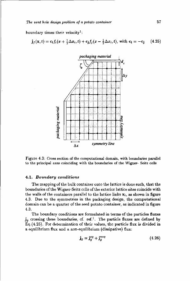
The vent hole design problem of a potato container 57

boundary times their velocity1:

j / ( x , i ) = afi(x+ ±Axi,t) + cifj(x- \&Xi,t), with Ci = - C J (4.25)

packaging material

5»

So

a

C ^

: !

i

• :

• i

•j •

1

1

:

I : i •

Ay

Ax symmetry line

Figure 4.3: Cross section of the computational domain, with boundaries parallel to the principal axes coinciding with the boundaries of the Wigner- Seitz cells

4 .1 . Boundary conditions

The mapping of the bulk container onto the lattice is done such, that the boundaries of the Wigner-Seitz cells of the exterior lattice sites coincide with the walls of the containers parallel to the lattice links x;, as shown in figure 4.3. Due to the symmetries in the packaging design, the computational domain can be a quarter of the seed potato container, as indicated in figure 4.3.

The boundary conditions are formulated in terms of the particles fluxes j s crossing these boundaries, cf. ref.1. The particle fluxes are defined by Eq.(4.25). For determination of their values, the particle flux is divided in a equilibrium flux and a non-equilibrium (dissipative) flux:

ig ~ Jg + J •neq (4.26)

58 Chapter 4

The equilibrium particle flux j gq is due to external velocity fields or force

fields. The non-equilibrium particle flux j ge q is due to density gradients,

and follows from a constitutive equation, such as Darcy's law, Fourier's law and Fick's law. The non-equilibrium particle flux at the boundaries of the computation domain is computed by taking the first order approximation of the constitutive equation:

%eq = 4>g(pg(xe)-p°g). (4.27)

Here, pg(xe) is the number density at the most exterior lattice site, p°g is the number density in the environment, and l/<j>g is the resistance to diffusion between lattice site at xe and the environment.

Symmetry lines At the symmetry lines the normal derivatives of all physical quantities are zero, and the normal components of the external force and velocities field are zero. This means, that at symmetry lines the lattice gas particle fluxes are zero:

jg = 0. (4.28)

This is achieved by reflecting all particles leaving the computational do­main: gin = gout.

Fluxes through packaging material As the packaging material of the potato container is impermeable to airflow, jy = pj\i = 0, the equilibrium heat and water vapour particle fluxes are zero, i.e.,

Jr"=«M/>9(xe)-p°]. (4-29)

The resistance to heat and water vapour diffusion, 1/<^9C, is a series con­nection of the resistance of the wall, \/<f)g

xt, and the resistance of the part of the Wigner Seitz cell, l/<j>g

nt, between the exterior lattice site at xe and the container wall1:

1 1 1

JZ^W^W' (4'30)

Here, <f>gnt — Dg/^Axe, and <j>ex* = agtC/dc. Dg is the diffusivity of the

particular lattice gas, as defined by Eq.(4.16). | A x e is the distance between the exterior lattice site at xe and the boundary. The diffusivity of the packaging material is a9tC. The thickness of the container walls is dc.

Some sidewalls of the containers are not parallel to one of the lattice links Ax,-. The x- and y-component of the heat and water vapour particle

The vent hole design problem of a potato container 59

fluxes are described with j 3 i Q = <f>giCl(pg(xe) — p°g), cf. ref.1. Here, the following definitions are used:

l / ^ , „ = l/fg% + l/<j>g% (4.31)

with

4>gnt

a = Dg/Axa, (4.32)

</>% = cos(C)ag,c/dc, (4.33)

4% = sin(C)a5,c/dc. (4.34)

Here, £ is the angle of the skew wall with the x-axis, as shown in figure 4.3.

Fluxes through vent holes At the vent holes with inward airflow, the heat and water vapour fluxes are described by:

j*0'e=p2u + pjHMx e)-$. (4-35) The equilibrium particle flux convects outside air with density p°g into the container. The velocity u is determined by means of the mass flux j / cross­ing the boundary of the computational domain, which can be computed with Eq.(4.25). The non-equilibrium fluxes are proportional to <j>g

nt, as there is no packaging material at the vent holes.

At vent holes with outward airflow, the heat and water vapour fluxes are described by:

Shg°

u = Pg(xe)u. (4.36)

Here, the non-equilibrium part is zero, as stated by the boundary condi­tion Eq.(4.11). The equilibrium particle flux convects air from inside the container with density pg(xe) into the environment.

The mass flux through the vent hole is described by:

j ; = pj (Xe)ue* + < ^ [ M * e ) " P°f(z)}. (4.37)

The equilibrium mass flux follows from Eq.(4.18). The internal reciprocal resistance is <$>%T,t = C?K/^) a s follows from Darcy's law Eq.(4.7) and the definition of the pressure, p = c^pj.

Fluxes through permeable packaging material Vent holes, with di­mensions smaller than the lattice spacing Az,-, are modelled as porous wall material. The particle flux through the porous wall has a contribution from the flux through the vent holes and a contribution from the flux through the packaging material:

3g=tc3hg0,e + (l-ec)%a". (4.38)

60 Chapter 4

Here, ec is the porosity of the wall material, which is equal to the ratio of the vent hole area and the area of the exterior surface of the Wigner- Seitz cell.

5. Condensation of moisture during cooling conditions

For validation of our LB scheme, cooling experiments are performed with existing designs of the seed potato containers. The designs investigated are:

• Octabin # 1 , a container with 5 vent holes in 4 side walls, and

• Octabin # 2 , a closed container without vent holes.

These designs are drawn schematically in figure 4.4. Both designs have a ground floor of 1.20 m by 1.00 m and a height of 1.60 m. The thickness of the corrugated board is 14 mm. The vent holes have a diameter of 30 mm. The vent holes are placed in the skew sidewalls such, to prevent blockage of the holes during transport by adjacent containers.

The octabins are filled with 1000 kg of seed potatoes, having a diameter ranging from dp=35 mm to rfp=55 mm. The initial temperature of the potatoes is 8°C. The filled octabins are stored in a cold room, controlled at -3°C and 85% relative humidity (R.H.) for 2 days. During this experiment the potato temperature is measured at various locations, as well as the relative humidity in the top of the octabin, and the amount of condensed moisture at the top layers of the potato load.

The experimental results show, that for both containers the R.H. at the top of the containers remained at saturated level for the whole period of 2 days. This is due to the occurrence of moisture condensation. At the end of the experiment in both containers, the condensed moisture is found largely in the top layer of potatoes up to a depth of approximately 12 cm. There has also been a small amount of moisture condensed on the inner liner of the corrugated board of the sidewalls. The amount of condensed moisture has been 147±15g for octabin # 1 , and 115±15g for octabin # 2 . Condensed moisture is not observed in the layers with a depth of 20-60 cm. Other layers have not been inspected. The time evolution of the measured temperatures are in compliance with our previous experiments and numerical simulations1, and will not be discussed in detail again.

With the LB scheme the behaviour the potatoes in the octabins during the cooling experiments is simulated. The values of most parameter values are set equal to known values from the previous model study1, and from material properties (Dc=2.9 10 - 6 m2/s). The yet unknown parameters are ftam and flap- At very low velocities, the assumption is justified9 that the

The vent hole design problem of a potato container 61

TenpeottuE C )

0.00 0 .30 0 .60

Distance from cen t re (m)

level { f t ) 1 - sT^£*"- . - ^ i ~ l 1 , 6 1

lie. _ i.211fc; y t T 4 _ * - \ „ i.: t

Ai r v e l o c i t y 6 mm/s = t

>C

^ 0 .0 0 .3 0 . 6

Distance from cen t re (m)

0.0 0.3 0.6

Distance from centre (m)

Distance from centre (m)

Octabin #1 Octabin #2

Figure 4.4: The temperature, R.H. distribution and velocity field in the vertical diagonal cross section after two days of cooling for the standard octabin and the closed octabin

Sherwood number Sh = /3amdp/D=2, from which /3am can be calculated. The coefficient for mass transfer from potato to air /?op depends strongly on the cultivar of potatoes and the time of the season, so it must be determined by trial simulations. From these simulations it is estimated that /?ap=5 10 - 5

m/s, which is of the same order as the value reported in literature9.

The simulations are performed with a lattice measuring 8 by 8 by 33 sites, and a time step At=3 s. By the application of the Lattice BGK scheme, the boundary conditions and steep gradients in the velocity field induce some small damped spurious oscillations, which also occur in other numerical schemes dealing with convection-diffusion problems12. The os­cillations are damped to an acceptable level if a Lattice Boltzmann scheme with a more general collision matrix, Qf-, is used. This scheme is the so-

62 Chapter 4

called enhanced collisions LB scheme2,11,7. A more detailed study on the reduction of these spurious oscillations will be performed in a subsequent paper13.

The numerical results of calculations using the above mentioned pa­rameter settings, are shown in figure 4.4 and 4.5. The distribution of the R.H., temperature and the airflow velocity field in the vertical diagonal cross section after two days of cooling are displayed in figure 4.4. In fig­ure 4.5 the amounts of condensed moisture are shown. As one can see the numerical simulation has reproduced the phenomena observed during ex­periments quite well: 1) only in the top layer the R.H. level is saturated and 2) moisture has condensed, with amounts that are in agreement with the experimental data (147±15g for octabin # 1 and 115±15g for octabin #2) .

The occurrence of condensation in the top layer of potatoes can be explained by taking the airflow and temperature distribution into account, as indicated in figure 4.4. In the centre of the octabin there is an uprising airflow that is warm and highly humid, due to the heat and mass transfer from the potatoes to the air. In the top layer this uprising airflow meets a sudden decrease in temperature. As the concentration, cs

aat, of saturated

water vapour decreases with temperature, the air becomes oversaturated and the excess water vapour condenses.

In the closed octabin (design #2) the condensation occurs across the whole top layer of potatoes, whereas in octabin # 1 with vent holes the condensation occurs only near the walls and the upper vent holes. These locations are indicated in figure 4.4 as regions with a R.H. level of 100%.

The displacement of the regions of condensation and the amount of condensed moisture in octabin # 1 , as compared to the closed octabin #2 , are explained by the difference in airflow pattern. In octabin # 1 the upper vent holes draw the uprising airflow in the centre of the container towards the sides of the octabin. Hence, it condenses in regions away from the centre, i.e., near the side walls and the vent holes. As the decrease in temperature near the sides is larger than in the centre of the box, the amount of condensed moisture is larger.

6. Numerical analysis of alternative vent hole designs

From the experimental and simulation results, described in the previ­ous Section, it is clear that the vent hole design of octabin # 1 does not decrease, but instead, increase the amount of condensed moisture, as com­pared to the octabin without vent holes. The simulations have shown, that the vent hole design changes the airflow pattern inside the container, and subsequently changes the temperature and humidity fields. By placing vent

The vent hole design problem of a potato container 63

150

o 5 -a

o O

Figure 4.5: The amounts of condensed moisture inside the various containers with vent holes after two days of cooling

holes in other locations, the internal airflow may be redirected such, t ha t the condensation of moisture is reduced. This is investigated by performing simulations with octabins, having alternative vent hole designs.

The alternative vent hole designs investigated are:

• Octabin # 3 with 26 holes distributed uniformly in the lid.

• Octabin # 4 with 26 holes distributed uniformly at bo th the lid and bo t tom.

• Octabin # 5 with 26 holes distributed uniformly at both the lid and bot tom, and with 5 holes distributed at different height a t the four side walls.

The vent hole designs are also drawn schematically in figure 4.5. All vent holes have a d iameter of 30 m m . The heat and mass transfer during cool­ing conditions is computed for all alternative vent hole designs. The initial and environmental conditions are taken equal to those of the cooling ex­periments. The size of the lattice and the t ime step are taken equal to the

64 Chapter .

values of the previous simulations with designs # 1 and # 2 . The computed results for the alternative vent hole designs are shown in figures 4.5 and 4.6. Figure 4.6 shows the R.H., temperature and velocity field in the vertical diagonal cross section at the end of the cooling experiment.

Temperature (C)

R.H. level (%)

Air velocity 6 mnVs = t

00 03 Distance to centre <m)

Octabin #3

03 06

Distance to centre (m) Distance to centre (m)

Octabin #4 Octabin #5

Figure 4.6: The temperature, R.H. distribution and velocity field in the vertical diagonal cross section for various alternative vent hole designs

The explanation for the performance of each vent hole design can readily be deduced from the simulation results concerning temperature, R.H. and airflow velocity.

The performance of octabin # 3 is similar to that of the closed container, octabin # 2 . The distributions of R.H., temperature show the same pattern, and the amount of condensed moisture is also comparable. This equal per­formance is explained by the nearly identical airflow patterns. There is very little air exchange through the vent holes in the top of the container. Vent

The vent hole design problem of a potato container 65

holes at different heights are needed for enhancement of the air exchange with the environment by buoyancy, as shown by the designs octabin # 1 , # 4 and # 5 .

Figure 4.6 shows, that the vent hole design of octabin # 4 reduces the amount of condensed moisture. The reduction is achieved by the placement of the vent holes in the top of the container and the bottom of the container. The suction vent holes in the bottom mainly draw cold and dry air from the outside. Whereas, the holes in the top mainly exhaust warm and humid air. The suction of cold dry air at the bottom lowers the R.H. level in the container, as compared to the previous designs. By locating the exhaust vent holes at the top of the container, the location with the highest risk of condensation, the accumulation of moisture in the top layer of potatoes is effectively prevented.

The little condensation, that occurs in octabin # 4 , is located at the top of the sides of the container. Along the inner side of the walls of the container there is a downward airflow, drawing some warm humid air from the centre of the container. The air gets oversaturated in the cold spots near the top of the container walls, and condenses there.

In octabin # 5 no condensation of moisture occurs. In comparison to octabin #4 , this design has vent holes in the sides. Because of these vent holes there is no downward airflow along the sides. Due to vent holes at different heights in the sidewall, the airflow along the sides is mainly upward. At the top of the container no air is drawn from the centre to the sides. The action of both these processes result in the absence of condensed moisture.

7. Conclusions

In this paper a Lattice Boltzmann scheme is presented, that describes heat and mass transfer in porous media by natural convection. By com­puting the heat and mass transfer behaviour of various container Designs with the LB scheme, the vent hole design problem of a container for 1000 kg of seed potatoes has been solved.

Simulations in this study and the previous study1, show that the model is well able to predict the experimentally observed heat and water vapour transfer in seed potato containers during cooling conditions, as occur during road transport.

Performing simulations with various containers having new vent hole designs, a seed potato container is found, in which no condensation occurs during the cooling conditions of road transport. This container has vent holes in the top, bottom and the sides. These vent holes draw cold dry outside air through the bottom and the sides, and exhaust warm and humid

66 Chapter 4

air at the top. This airflow prevents the accumulation of water vapour, and subsequently the condensation of moisture. As condensed moisture, the biggest threat for the pota to keeping quality, is absent, the seed potatoes can safely be t ransported in this container. If the seed po ta to containers will be used for storage after road t ransport , the developed LB scheme can be used for further optimisation of the vent hole design towards reduction of weight loss. In storage weight loss is also of importance for the keeping quality.

From the performance of the various container designs, as shown by the Simulations, some guidelines can be s tated concerning the design of vent holes in bulk containers. These guidelines are:

•

•

•

Vent holes should be placed at different heights, for enhancement of air exchange with the outside.

Exhaust vent holes should be placed nearest to the regions with high risk of condensation of moisture.

Suction vent holes should be placed as low as possible for aeration of the whole container.

By placing extra vent holes in the side walls at different heights one achieves upward flow throughout the container, which minimises the risk of condensation.

Regions with high risks of condensation, and the possible locations of ex­haust and suction holes, can be estimated best from the behaviour of a closed container without vent holes.

Given these results presented in this paper - the solution of the vent hole design problem and the design guide lines - it can be concluded, tha t the Lattice Boltzmann scheme is a useful tool for obtaining adequate solutions to engineering problems, such as the design of vent holes in bulk contain­ers. The LB scheme is able to simulate both the heat and mass transfer phenomena as occurs in bulk containers.

1. R.G.M. van der Sman, Lattice Boltzmann scheme for natural convection in porous media. Int. J. of Modern Physics C, 8 (4): 879, (1997); Chapter 3.

2. R. Benzi, The lattice Boltzmann equation: theory and applications. Phys. Rep. 222 (3): 145,(1992).

3. J.M.V.A. Koelman, A Simple Lattice Boltzmann Scheme for Navier-Stokes Fluid Flow. Europhys. Lett. 15: 603, (1991).

4. J.G.M. Eggels, and J. A. Somers, Numerical simulation of free convective flow using the lattice-Boltzmann scheme. Int. J. Heat and Fluid Flow 16: 357, (1995)

The vent hole design problem of a potato container 67

5. E.G. Flekkoy, Lattice BGK Model for Miscible Fluids. Phys. Rev. £ 4 7 : 4247, (1993).

6. R.G.M. van der Sman, et. al., submitted to Int. J. of Heat and Mass Transfer, (1998).

7. R.G.M. van der Sman and M.H. Ernst, Diffusion Lattice Boltzmann scheme on an orthorhombic lattice. / . of. Stat. Phys., 94 (1/2): 203-217, (1999); Chapter 5.

8. F.W. Bakker-Arkema, Simultaneous Heat and Mass Transfer during the Cool­ing of a Deep Bed of Biological Products under Varying Inlet Air Conditions. J. Agr. Eng. Research 12 (4): 297, (1967).

9. K.J. Beukema, Heat and mass transfer during cooling and storage of agri­cultural products as influenced by natural convection. Ph. D. Thesis, Agr. Univ., Wageningen, the Netherlands. (1980)

10. K.K. Khankari, S.V. Patankar and R.V. Morey, A mathematical model for natural convection moisture migration in stored grain. A SEA paper no. 93-6017., (1993).

11. O. Behrend, R. Harris, and P.B. Warren, Hydrodynamic behaviour of lattice Boltzmann and lattice Bhatnagar-Gross-Krook models, et.al., Phys. Rev. E, 50 (6): 4586, (1994).

12. C. Johnson, Numerical solution of partial differential equations by the finite element method, Cambridge University Press, 1987.

13. R.G.M. van der Sman, Convection-diffusion Lattice Boltzmann scheme for Bravais and irregular lattices. J. Comp. Phys., submitted 1999; Chapter 6.

Chapter 5

Diffusion scheme on an or thorhombic lattice

1. Introduction

The Lattice Boltzmann scheme is a recently developed technique for modelling physical transport phenomena1. The algorithm is quite simple and is derived from basic physical principles. Because of its simple nature, it is frequently, and successfully used for modelling complex phenomena, such as hydrodynamics, multi-phase flow, natural convection and reaction diffusion2-6. As the method is relatively new, most studies are done with high symmetry lattices, such as the cubic and square lattice. However, engi­neering problems may demand the use of less symmetric lattices. Regarding this problem few studies have been performed. This problem is investigated by analysing the Lattice Boltzmann scheme, that models isotropic diffusion on an orthorhombic lattice, with different lattice spacing in the three or­thogonal directions.

Diffusion has rarely been the prime focus of studies using LB schemes7, although it is a simple phenomenon from both a mathematical and nu­merical point of view. Isotropic diffusion in a homogeneous medium is mathematically described by the following elliptic partial differential equa­tion:

8tPg = DV2Pg. (5.1)

Here, pg is the diffusing physical quantity and D is the diffusion coefficient.

to appear as: R.G.M. van der Sman, and M.H. Ernst, Diffusion Lattice Boltzmann scheme on an Orthorhombic Lattice. J. of. Stat. Phys., 94 (1/2): 203-217, (1999).

69

70 Chapter 5

The solution of elliptical partial differential equations does not pose many problems for conventional numerical methods8. It is conceivable that this is also the case for Lattice Boltzmann schemes. Hence, diffusion is an ideal problem for detailed theoretical analysis of the LB scheme and for inves­tigations directed towards generalisation and optimisation of the method. Furthermore, it is expected, that improvements of the Lattice Boltzmann technique found for diffusion can lead to new applications for more complex phenomena such as fluid flow.

In order to find all possible degrees of freedom, which can be used for improving the Diffusion LB scheme (DLB) is constructed from first principles, i.e., the conservation laws and lattice symmetry requirements. The properties of the DLB scheme concerning consistency, stability, and accuracy are analysed in terms of eigenmodes9'10. Using the eigenmode analysis, we investigate ways of improving the performance of the DLB scheme using its extra degrees of freedom.

2. Lat t ice Bo l t zmann scheme

2 .1 . Lattice Boltzmann Equation

The general formulation of the Lattice Boltzmann scheme, can be writ­ten as cf. ref.1:

gi(x + CiAt,t + At) = gi(x,t) + Qij[gejq(x,t)-9j{x,t)] = Aijgj{x,t). (5.2)

Here, the distribution function gi(x,t) represents the number of particles on lattice site x at time t, moving with velocity c,-. The velocities are chosen such that at the next time step t + At the particles move to neigh­bouring sites x + Ax,, hence c; = Ax, /At . Here, geq is the local, single particle, equilibrium distribution. In the case of diffusion the equilibrium distribution is a weighted function of the density pg{x, t) = J2i <7i(x> *)> i-e-> g°q(x,t) = Wipg(x,t). The weight factors depends on the geometry of the lattice and will be specified below. Furthermore, Q,j is a relaxation matrix. The matrix elements Aij are the transition rates between states, which are associated with a particular velocity c,. This formulation of the LB equation, Eq.(5.2), is also known as the enhanced collisions LB scheme1.

The standard requirements11 for any LB collision operator are: (1) the transition rates are normalised, which guarantees that the collisions are conserving the number of particles, and (2) the collision operator must allow a collision invariant equilibrium distribution g^q. These requirements impose:

7 .A? 1, (5.3)

Diffusion scheme on a orthorhombic lattice 71

EA^T = 9?- (5-4)

2.2. Symmetries

In order for the Lattice Boltzmann Equation to describe the desired physical phenomena, the lattice and the collision operator should have cer­tain symmetries, cq. invariances. In case of isotropic diffusion the con­straints are: i) the collision operator is invariant under all isometries of the Bravais lattice, and ii) second rank tensors are isotropic. The constraint ii) guarantees that the diffusivity tensor Dap is isotropic, i.e., reduces to DSa/3. The standard definitions, Eqs.(5.3-5.4), combined with constraint ii) impose the following conditions on g^12:

Y.^ = P9> (5-5) i

5> , a r f ' = °> (5-6) i

53c».ac»'.^,-9 = PgCt&ap- (5-7) i

The constant c2. is related to the metric of the Bravais lattice. For fluid flow problems it is identified as the speed of sound of the lattice gas. For diffusion problems, it has no direct physical meaning.

Investigation of the conditions Eqs.(5.5)-(5.7) shows that they are satis­fied on a lattice with principal axes having two-fold rotation symmetry. In three dimensions the lattice gas can reside on an orthorhombic lattice with lattice spacings Axa = caAt, which are in general unequal. Each lattice site has six states, corresponding to the velocity vectors connected to the six nearest neighbouring sites, defined as Cj = —c,-+3 = ca. The orthorhombic lattice and its associated particles velocities are drawn in figure 5.1.

Eqs.(5.5)-(5.7) are indeed satisfied by a weighted function of the number density: g^q = u>ipg. The weight functions are given by:

c2 1 v-v 1 Wi= 2 ^ ' w i t h ? = X,2^- (5-8)

72 Chapter 5

t

. # - •

* — — 1

II

» ;;t

. # • ' • • '

i-—; i

> 1

. r<.

< ,< » ' •

( • — ' • — <

i <

i : *

«'' ('

:• —*' j

C5 '

a Figure 5.1: The six-velocity orthorhombic lattice.

2.3. Collision matrix

Taking into account the two-fold rotation symmetry of the orthorhom­bic lattice, one can formulate the most general expression for the collision matrix A-,-:

(5.9)

Note that the collision matrix is in general not symmetric, i.e., Aap ^ Apa. The collision matrix is fully characterised by its eigenvalues fj.a and

eigenvectors va<i, where the right and left eigenvectors are respectively de­fined as:

/ An A2i

A31

Bn -421

V A31

A12

A22

A32

An B22

A32

A13

A23

A33

A13

A23

B33

Bu A21

A31

Au

A21

A31

A12

B22

A32

A12

A22

A32

A13

A23

B33

A13

A23

A33

\

/

/ 1 AjjWjVqj — fl>awiva,i,

3

(5.10)

(5.11)

Using this definition we can construct the eigenvectors, following the pro­cedure in ref.13.

Diffusion scheme on a orthorhombic lattice 73

The first eigenvector follows directly from the standard requirements, Eqs.(5.3)-(5.4), which are satisfied if there exists an eigenvector with

Ho = 1 ; v0,i = 1. (5-12)

This is the so-called density mode eigenvector, the left eigenvector is com­monly denoted as < 1|. The density follows from projecting the state vector <7,- onto the eigenvector, meaning that p = < 1|<; >.

Next, there are three eigenvectors < va\ of odd parity under inversion of all velocities (c* —>• —c,-). These so-called flux modes can be related to Carte­sian components of the gradient in the number density dap ~ < va\g > . In order to have an isotropic diffusion, the corresponding eigenvalues must be equal (3-fold degenerate):

fia = A ; va,i = Ci<a. (o.lo)

The remaining two eigenvectors have even parity under velocity inver­sion, and can be related to second order derivatives of the number density. The corresponding eigenvalues must be equal (2-fold degeneracy) to guar­antee isotropic diffusion, requiring:

pa+p = K ; va+/3,i = cja - c2iiP, with 0 ^ a. (5.14)

All eigenvectors and corresponding eigenvalues are listed in Table I. After some lengthy, but straightforward algebra using the eigenvalue

equations, one finds the expressions for the components of the collision operator:

Aaa = wa(l- K) + ~(K + X),

Aap — wa[\ — K), with a ^ j3,

Baa = Wa(l-K,) + -(K-\).

(5.15)

(5.16)

(5.17)

It is readily seen that the two-fold symmetry of the lattice and the standard requirements, Eqs.(5.3)- -(5.4), are satisfied, and that the collision matrix meets the detailed balance condition:

AijWj = AjiWi. (5.18)

Therefore, we have shown that the imposed lattice symmetries together with the implied isotropic diffusion imply the detailed balance condition Eq.(5.18).

74 Chapter 5

Table I Eigenvectors va and eigenvalues of the the DLB scheme fifLB and Lattice BGK scheme (iBGK

a

0

1

2

3

4

5

V a

< 1

< Ci

< 0

< 0

< c2

< 0

1

0

C2

0

-c2

c2

1

0

0

C3

0

-c2

1

-c\

0

0

c2

0

1

0

-C2

0

-c2

c2

1

0

0

-c3

0

-c2

..DLB ra

1

A

A

A

K

K

..BGK ra

1

1 -U

1 - W

1 - W

1 - W

1 - W

Having obtained the expression for the collision operator, we have the most general diffusion Lattice Boltzmann (DLB) scheme. The DLB scheme has two degrees of freedom, eigenvalues A and K, and is valid on lattices with only two-fold symmetry, which holds for the orthorhombic lattice in three dimensions.

The DLB scheme has an extra degree of freedom over the traditionally used Lattice BGK scheme14. The DLB scheme becomes equal to the BGK scheme when setting A = K = 1 — u>. For comparison, the set of eigenvectors and eigenvalues for the BGK scheme are also listed in Table I. Hence, the Lattice Boltzmann equation for the BGK scheme is written as:

gi(x + ciAt,t + At) = gi(x,t)+uj[geiq(x,t)-gi{x,t)]. (5.19)

In order to be consistent with existing literature, we use below l—ui instead of A for the notation of eigenvalues of the flux modes.

Diffusion scheme on a orthorhombic lattice 75

3. Eigenmode analysis

3.1. Eigenmodes

Having constructed the diffusion Lattice Boltzmann scheme with a col­lision operator Aij satisfying all required symmetry properties, the consis­tency, stability and accuracy are determined by analysing the LB equation Eq.(5.2) in terms of eigenmodes9. This approach is very similar to the traditional von Neumann stability analysis of numerical schemes.

Assuming an unbounded or periodic lattice, the eigenmodes of the Lat­tice Boltzmann equation are given by:

gt{x,t) = gi(k)exp(st + ik • x), (5.20)

Here s = s(k) is the relaxation rate of the eigenmode. Substitution of the ansatz Eq.(5.20) into the LB equation Eq.(5.2) leads to the eigenvalue equation:

exp(- ik • Axi)A,j^(k) = exp(s(fc)Ai)<7,(k). (5-21)

From the spectrum of the eigenvalues fi(k) = exp(s(k)At), information about the consistency, stability and accuracy can be deduced. The number of eigenmodes of the LB equation is equal to the number of states at a lattice site. The eigenmodes can be divided in slow modes, related to conservation laws, and kinetic modes, which usually decay rapidly9,10. As diffusion is only concerned with conservation of mass, the DLB scheme has only one slow diffusive mode. The scheme will show diffusive behaviour if the relaxation rate of the diffusive eigenmode is significantly slower than that of the kinetic modes.

The LB scheme is consistent with diffusion if for the dominant (diffusive) eigenmode it holds that i?e(s(k)) ~ —Dk2 and 7m(s(k)) = 0. Then the time evolution of the number density will be:

pg(x,t) = ^ # , ( x , £ ) = p0exp(-Dk2t)exp(ik -x), (5.22) i

as follows from the Laplace transformation of Eq.(5.1). The diffusion coef­ficient D depends on the eigenvalues of the collision operator Aij and will be derived below by means of the perturbation analysis of the eigenvalue equation.

3.2. General properties

The properties of the LB scheme are discussed using a simple case, for which there is an analytical solution for the eigenvalue problem Eq.(5.21).

76 Chapter 5

The case studied is that of a Lattice BGK scheme applied to a cubic lattice for eigenmodes having wave vectors equal t o k = A ( l , l , l ) . The correspond­ing eigenvalue equation is solved using the algebraic manipulation software package Maple™:

A*o,i(fc) = ( l - ^ ) c o s ( ^ ) ± [ ( l - i w ) 2 c o s 2 ( f c ) + ( W - l ) ] ^ (5 .23 )

H2i3(k) = ( l -w )exp (+ i* ) (5.24)

/i4|5(fc) = (1 — w)exp(—ik), (5.25)

The properties of the LB scheme follow from the spectrum of the eigen­values , as shown in figure 5.2. The dispersion relations are qualitatively similar to those of hydrodynamic LB schemes10, and therefore the proper­ties presumably hold for LB schemes in general. These properties are:

• The LB scheme has one single diffusive mode decaying, for small k, at a rate s(k) = —Dk2. It is dominant over the kinetic modes for a wide range of wavelengths k in the range of 1 < w < 2.

• The LB scheme is unconditionally stable, i.e., \Re(fj,a(k))\ < 1 holds for all eigenmodes.

• In the range of 0 < u < 1 the diffusive behaviour of the scheme is limited. At relatively large wavelengths the diffusive mode becomes mixed with a kinetic mode.

• In the range of w —• 2, the diffusive mode is not dominant over all kinetic modes. Consequently, the LB will show spurious oscillations due to slowly damped (oscillating) kinetic modes, i.e., Re(fxa(k)) —» — 1 and Im(/j,a(k) ^ 0).

Take note, that these properties hold only for unbounded or periodic lat­tices. For finite lattices the results found, will be valid for the inner part of the lattice. Near and at the boundaries the effects of the boundary conditions become significant. Sharp gradients at the boundaries induce instabilities or spurious modes, which cannot be captured with this eigen­modes analysis.

3.3. Perturbation analysis

As diffusive behaviour is obtained in the long wave length regime (A: < 1), we can determine the accuracy of the LB scheme by expanding the eigenvalue equation Eq.(5.21), cf. ref.9, in powers of the wave vector of

Diffusion scheme on a orthorhotnbic lattice 77

or

1.U

o.o-

i.oH

>~- (0=0.25

1 I ' I ' I

co = 0 . 2 5

CD EC

-1.0

0) LX

a) EC

-1.0 1 ' 1 •—

0.0 1.0 2.0 3.0 k

1.0

¥ 00

-1.0

(0=1.25

i ' I ' r 0.0 1.0 2.0 3.0

k

i "

E

I .U

o.o-

-i.oH

io=1.75

1 I ' I ' I

0.0 1.0 2.0 3.0 k

Figure 5.2: The spectrum of eigenvalues of a Lattice BGK scheme for w=0.25, 0.75, 1.25 and 1.75 applied on a cubic lattice, with Ai,- = 1. The wave vector of the eigenmode is k = (k,k,k). The thick solid line is the dispersion relation of the eigenvalue fio of the diffusive mode. The dashed line represents the dispersion relation for eigenvalue //!. The other dispersion relation are shown as thin solid lines. Observe that the diffusive mode for u — 0.75 and u> — 0.25 becomes a propagating kinetic mode at finite A;.

78 Chapter 5

length k, and having an arbitrary direction. Furthermore, this perturba­tion analysis gives us the relation between the diffusion coefficient and the relevant eigenvalue of the collision operator.

In this analysis, the wave-vector expansion is applied to the particle distribution gi and the relaxation rate s:

&(k) = ^ 0 ) + ikgV + (ik)2g\2) + 0(k3), (5.26)

«(*) = (»7fc)si + {ik)2s2 + {ik)3s3 + <D(k4). (5.27)

The particle distribution function is expanded as a series of perturbations jji' around the equilibrium distribution g\ ' = g\q. As there are no prop­agating modes for the diffusion problem, see figure 5.2, the eigenvalue s(k) is an even function of the wave number, i.e., s\ = 0 and S3 = 0.

After substitution of the expansions, Eq.(5.26)-(5.27), in the eigenvalue equation Eq.(5.21) and performing a Taylor expansion, one obtains:

^ , ( 1 ) ( k ) = - ^ ^ ( 0 ) (5.28) CO

(ik)2g\2\k) = -j^-i 1 - i)[(fk • Ax,)2 - ( ;* ) 2A^(°) (5.29)

where Ax2. = c2At2. For S2 one finds:

s2 = c2s{--\). (5.30)

Hence, the relaxation rate of the diffusive mode is s ~ —k2D + 0(k4). The diffusion LB scheme is accurate up to the third order in the wave number k. The expression for the diffusion coefficient in Eq.(5.30), i.e., D = C2(1/OJ — l/2)At, is identical to the one for the Lattice BGK scheme on a cubic lattice7. The diffusion coefficient depends only on the eigenvalue of the flux modes. The effects of the different lattice spacing are totally

4. Opt imisa t ion of t h e DLB scheme

4 .1 . Free parameter K

As is shown above, the diffusion coefficient depends only on the eigen­value of the flux modes 1 — w. This means that the eigenvalue K of the collision operator can be used for optimisation of the consistency and ac­curacy of the LB scheme.

An obvious choice for the free parameter K is to set it to zero, so that the associated kinetic modes will die out immediately1,10. It is expected

Diffusion scheme on a orthorhombic lattice 79

DC

Q

<D DC

DC

i "

E o.o-

-1.0

01=0.25

- ^ " ^ X -v ,̂/ 1 ' 1 ' 1

0.0 1.0 2.0 3.0 k

i

E

I .U

o.o-

-i.oH

O)=0.75

I ' I ' I

0.0 1.0 2.0 3.0 k

-1

"F

l .U

o.o-

-1.0J

o> = 1 2 5

I ' I 1

0.0 1.0 2.0 3.0 k

DC

0.0

1.0

-^ 0.0

— i — ' i '—r 0.0 1.0 2.0 3.0

k

-1.0

m.=-1-Za.

— i — ' — i — ' — r 0.0 1.0 2.0 3.0

k

Figure 5.3: The spectrum of eigenvalues at k = (k, 0,0) of the BGK scheme (dashed lines) and the DLB scheme (solid lines) for O J = 0 . 2 5 , 0.75, 1.25 and 1.75 applied on a cubic lattice with A a;,- = 1. In the left par t of the figure the ratio of the real part of the relaxation Coefficient of the diffusive mode Re(s) and the theoretical dispersion relation s — —Dk2 is shown. In the right part the imaginary part of the eigenvalue Im(fj.) for all eigenmodes are shown.

80 Chapter 5

that this choice of K = 0 will lead to improved diffusive behaviour. This hypothesis is checked numerically, by comparing the spectra of the eigen-modes for the DLB scheme with those for the Lattice BGK scheme. The spectra are computed for k = (k, 0,0) and for four values of the relaxation parameter u>. The plots of the spectra are shown in figure 5.3.

The ratio between the computed value of the relaxation rate and the theoretical value (s(k) = —Dk2) is shown in the right part of the figure 5.3. Deviation of this ratio from 1 means deviation from diffusive behaviour. Indeed, one observes from figure 5.3 that the DLB scheme has improved diffusive behaviour over the BGK scheme, because for w > 3/4 the relax­ation rate s(k) = —Dk2 for a larger range of wavelengths. One observes in the left part of figure 5.3 spurious propagating modes, occurring in the BGK scheme. These modes are absent in the DLB scheme. For all eigenmodes Im(s(k)) = 0 in the range of w > 3/4. It must be noted that elimination of spurious modes occurs only for certain directions of the wave-vector. If k = (k,k,k) the flux modes will show oscillating behaviour, which is not eliminated by setting « = 0.

a <u

1 . 2 -

1.1 -

1 . 0 -

0 . 9 -

0.8 - |

0

1 . 2 -

1.1 -

1 .0-

0 . 9 -

0 . 8 -

0

(0=1.25

_..-**

~">v \

\ \ \

1.0 2.0 3.0 k

' / (0=1.75 / / • ..-'

>;.--

0.0 1.0 2.0 3.0 k

Figure 5.4: The ratio of the real part of the relaxation rate of the dif­fusive mode Re(s(k)) over the theoretical value —Dk2, as a function of the normalised wavenumber kAx. The wave vector of the eigenmode is k = (A:, 0,0). Lattice spacings are Ax-(points), and At/ = Az = 1.

(solid lines), 1 (dashed lines), 2

Diffusion scheme on a orthorhombic lattice 81

4.2. Lattice spacing

Another way of improving the diffusive behaviour of the LB scheme is to increase the number of lattice sites along the direction of the density gradient Vpg. We show this by computing the spectra of the DLB scheme (with K = 0) for different lattice spacing along the direction of wave vector k = (k, 0,0). We have set Ax = \, 1, 2, and Ay = Az = 1. The computed spectra are shown in figure 5.4. Again, the ratio of the computed value and the theoretical value of the relaxation rate of the diffusive mode is plotted as a function of the wave number, for u = 1.25 and u = 1.75. This ratio is about 1 for a larger range of wave numbers for Ax = | , especially for high w. Consequently, the deviation from pure diffusive behaviour is smallest for Ax = | .

Hence, if there is prior knowledge about the gradients in the density field, the metric of the lattice can be optimised for that particular case. The lattice should be densified along the direction of the gradient. On the other hand, the lattice can be stretched along the opposite directions, such that the total number of lattice sites can be kept limited.

5. Discussion

A diffusion Lattice Boltzmann (DLB) scheme is constructed from first principles, i.e., lattice symmetry requirements and the conservation laws. Isotropic diffusive behaviour is obtainable from orthorhombic lattices with six different velocity states. The collision operator of the DLB scheme has two eigenvalues, of which only one is related to the diffusion coefficient. The other eigenvalue can be chosen freely and is used for improving the performance of the DLB scheme.

The procedure of constructing of the DLB scheme from first princi­ples can be equally well applied to other phenomena such as convection-diffusion and hydrodynamics. The Lattice-BGK schemes currently used for convection-diffusion and hydrodynamics, can be made more general, as indicated by the existence of a hydrodynamic LB scheme for 2-D rectan­gular lattices with nine velocities2, and the two-parameter LB scheme for hydrodynamics1 °.

The eigenmode analysis is a valuable tool for analysing the properties of the DLB schemes concerning consistency, stability and accuracy. The properties of the diffusion DLB scheme are:

• The behaviour of the DLB scheme is consistent with diffusion for a wide range of u> and wave number k.

• The validity of the DLB scheme is poor for 0 < u < 1.

82 Chapter 5

• The validity of the DLB scheme for u w 2 is l imited to low wave numbers. Sharp gradients, which occur near boundary conditions, will lead to spurious oscillations.

• The DLB scheme is unconditionally stable.

• The DLB scheme has at least second order accuracy.

• By setting free eigenvalues (K) equal to zero, both the range of con­sistency with diffusion and the damping of spurious oscillations are improved.

• The diffusive behaviour of the DLB scheme is improved if the lattice spacing is densified along the direction of the gradient.

These properties the DLB scheme hold also for hydrodynamic LB schemes10

and probably for LB schemes in general. Recent studies have recognised, tha t LB schemes are a special discreti­

sation of the classical Boltzmann equation1 5 , 1 6 . They show tha t other dis­cretisation schemes, as employed by the Finite Difference method, and ir­regular lattice spacing may equally well be applied to LB schemes. The construction procedure and the method of analysis presented in this pa­per can be valuable tools for investigation of the properties of such new schemes. It may be worthwhile to perform this investigation first for dif­fusion, as this is the simplest phenomenon tha t can be modelled with LB schemes, whilst the findings probably also hold for more complex phenom­ena as hydrodynamics.

1. R. Benzi, S. Succi, and M. Vergassola, The lattice Boltzmann equation: theory and applications. Phys. Rep., 222(3): 145-197, 1992

2. J.M.V.A. Koelman, A Simple Lattice Boltzmann Scheme for Navier-Stokes Fluid Flow, Europhys. Lett., 15 (6), 603-607, (1991).

3. E.G. Flekkoy, Lattice BGK Model for Miscible Fluids, Phys. Rev. E, 47, 4247-, (1993).

4. M.R. Swift et.al., Lattice Boltzmann Simulations of Liquid Gas and Binary Fluid Systems, Phys. Rev. E, 54 (5), 5041-5052, (1996). .

5. J.G.M. Eggels, and J. A. Somers, Numerical simulation of free convective flow using the Lattice Boltzmann scheme, Int. J. Heat and Fluid Flow, 15, 357-364 (1996).

6. S. Ponce-Dawson, S. Chen, and G.D. Doolen, Lattice Boltzmann computa­tions for reaction-diffusion equations, J. Chem. Phys. 98(2):1514-1523, 1993

7. D. Wolf-Gladrow, A Lattice Boltzmann Equation for Diffusion, / . Stat. Phys. 79 (5/6), 1023-1032 (1995).

8. C. Hirsch, Numerical computation of internal and external flows, John Wiley & Sons, N.Y., (1990).

Diffusion scheme on a orthorhombic lattice 83

9. S.P. Das, H.J. Bussemaker, and M. H. Ernst, Generalized hydrodynamics and dispersion relations in lattice gasses. Phys. Rev. E, 48 (1) (1993).

10. O. Behrend, R. Harris, and P.B. Warren, Hydrodynamic behaviour of lattice Boltzmann and lattice Bhatnagar-Gross-Krook models, Phys. Rev. E. 50 (6), 4586-4595 (1994).

11. U. Frisch, et.al., Lattice Gas Hydrodynamics in Two and Three Dimensions, Complex Systems 1, 649-707 (1987). See also, Lattice gas methods for partial differential equations, G.D. Doolen (ed), Addison-Wesley Publ. Co., p.75, (1989).

12. G. McNamara and B. Alder, Analysis of the Lattice Boltzmann treatment of hydrodynamics, Physica A, 194, 218-228, (1993).

13. R. Brito, M.H. Ernst, and T.R. Kirkpatrick, Staggered diffusivities in lattice gas cellular automata, J. Stat. Phys. 62, 283, (1992).

14. Y.H. Qian, D. d'Humieres and P. Lallemand, Lattice BGK Models for Navier-Stokes Equation, Europhys.Lett., 17 (6), 479-484 (1992).

15. X. He, L.S. Luo, and M. Dembo, Some Progress in Lattice Boltzmann Method. Part I. Non-uniform Mesh Grids, J. of Comp. Phys. 129, 357-363, (1996).

16. N. Cao, S. Chen, S. Jin, and D. Martinez, Physical symmetry and lattice symmetry in the lattice Boltzmann method, Phys. Rev. E 55 (1), R21-R24, (1997).

Chapter 6

Convection-diffusion scheme for irregular lattices

1. Introduction

In the last decade Lattice Boltzmann schemes have been successfully applied to the analysis of a variety of complex physical phenomena, such as turbulent flow, natural convection, and multi-phase flow1-4. Probably due to the complexity of the problem considered, the Lattice Boltzmann schemes have not yet been thoroughly compared to traditional numerical schemes, such as Finite Element and Finite Difference Methods. This com­parison becomes more feasible when considering less complex phenomena, such as diffusion and convection-diffusion. These phenomena have been addressed only recently5-8 .

The numerical solution of convection-diffusion phenomena presents seri­ous difficulties in cases where convection dominates over diffusion. Standard techniques like Galerkin Finite Elements or (Upwind) Finite Differences are plagued with either spurious numerical oscillations or high numerical diffusion11. These difficulties have been eliminated largely by dedicated, higher-order schemes like streamline-upwind Petrov-Galerkin (SUPG)12, or Crank-Nicolson Taylor-Galerkin (CNTG)13. These procedures are fairly complicated, and present a large hurdle for applying the schemes to practi-

submittedas: R.G.M. vander Sman, M.H. Ernst, Convection-diffusion Lattice Boltz­mann scheme for irregular lattices. J. Comp. Phys. (1999).

85

86 Chapter 6

cal engineering problems like solute t ransport in soils15 , vapour t ransport in textiles17 , drying and cooling of foods18 , 19 , and conditioning agricultural products in packaging systems6 , 7 , 9 . Often these problems require other phenomena, like porous media flow and moisture sorption, to be modelled. This makes the high-order schemes, which are especially dedicated to pure convection-dominated problems, less appropriate for the practical engineer­ing problems mentioned above.

In Lattice Boltzmann schemes physical t ransport phenomena are mod­elled in a very direct way, by having particles propagate from site to site on a lattice of grid points. After propagation, these so-called lattice gas particles collide with other particles, arriving at the same lattice site. If appropriate physical conservation laws are satisfied, and if the lattice pos­sesses some minimal degree of symmetry, the averaged behaviour of the lattice gas particles exhibits the proper physical behaviour2 0 .

Given the problems with s tandard Finite Element and Finite Differ­ence techniques and the complexity and specificity of high-order schemes on one hand, and the simplicity of the Lattice Boltzmann method on the other hand, we have applied the LB scheme as an alternative tool to solve convection-diffusion problems in packaging systems for agricultural prod­ucts. These applications have been quite successful. The LB schemes have reproduced experimental d a t a with a reasonable accuracy6 , 7 , 9 . Further­more, they have solved the moisture condensation problem in a packaging system for pota toes 7 .

The LB-scheme can exhibit numerical oscillations, as is found in the initial stage of the cooling of packaged agricultural p roducts 7 , 9 . In models, describing both heat and water vapour transfer, the oscillations can lead to artificial condensation of moisture, which is a numerical artefact and physically incorrect.

The aim of this paper is to investigate how the properties of the convection-diffusion Lattice Boltzmann scheme can be improved, such tha t problems, like spurious oscillations, are reduced. Two approaches are taken: 1) local refinement of the computat ional grid, and 2) increase of the accuracy.

The problem of refined grids has been addressed in a few papers 2 3 , 2 4 , 2 5 , using either coarse-graining or interpolation techniques. These techniques imply a significant departure from the t raditional framework of the Lattice Boltzmann scheme, thereby loosing their a t tractive properties. Moreover, they exhibit significant numerical diffusion and do not satisfy conservation laws26 .

In this paper, a LB scheme for convection-diffusion on irregular grids is derived, which does fit in the t raditional framework of LB-schemes, and therefore retains the attractive properties of the LB-schemes on regular lattices.

Convection-diffusion scheme for irregular lattices 87

The investigation is started with the derivation of a convection-diffusion scheme for Bravais lattices with improved accuracy, using the framework developed in refs.21'8. The key point of this framework is that the velocity moments of the equilibrium particle distribution function must equal those of the classical Maxwell-Boltzmann distribution.

For convection-diffusion it is sufficient that the velocity moments up to second order are satisfied4. In that case the scheme is Galilean invariant and will show little numerical diffusion. It has been shown that the constraints for the velocity moments are satisfied for highly symmetric lattices, such as the hexagonal lattice and the nine-velocity square lattice4,1,22.

Because we like to extend the Lattice Boltzmann methodology to irreg­ular grids, we will consider the more convenient lattices in d dimensions, having unit (Wigner-Seitz) cells with only two-fold rotational symmetry. Hereby, we extend our previous studies6,7 on convection-diffusion problems on orthorhombic lattices with 2d velocities. In this paper rest particles are also included, for which is shown that they improve the accuracy at the convection-diffusion scheme4.

The investigation is started with the deriviation of the convection-diffusion scheme for the orthorhombic lattice with 2d + 1 particle veloc­ities. Subsequently, a convection-diffusion LB-scheme is derived for irregu­lar lattices. Finally, both LB-schemes are compared with a number of the traditional Finite Difference and Finite Element schemes using benchmark problems, in order to assess the merits and shortcomings of the LB schemes.

2. LB scheme for orthorhomic lattices

In this section, a LB scheme is derived for convection-diffusion on or­thorhombic lattices. For the convection-difussion problems considered in this paper we assume: 1) isotropic diffusion and 2) an externally imposed velocity field, which is uniform and time-independent. Under these assump­tions the convection-diffusion equation reads:

dtPg+u-VPg = DV2pg. (6.1)

Here pg is the convected physical quantity, which can be a mass density of a tracer or an energy density, (i.e., temperature), u is the velocity field and D is the (thermal) diffusivity.

Lattice Boltzmann schemes describe convection-diffusion by the time-evolving particle distribution function <7,-(x,t). This function states the number density of particles at lattice site x and time t moving with velocity c, = Ax,-/At along the lattice link connecting the sites x - A x ; and x. The dynamics on the macroscopic scale is then obtained by summing the particle distribution over all states, i.e., the density is pg(x,t) = ^,-</i(x,t).

88 Chapter 6

At each time step, the lattice gas particles propagate to neighbouring lattice sites, where they collide with other particles. Furthermore, the par­ticles can change their momentum through externally imposed fields, such as the velocity field in the convection-diffusion problem. The propagation and collisions of lattice gas particles are described by the so-called Lattice Boltzmann equation, which is a discretisation of the classical Boltzmann equation, having a linearised collision integral. In its most general formu­lation the Lattice Boltzmann equation reads:

# ( x + Ax,-, t + At) - 9i(x, t) = ^ « y [#(*• t) - g?(x, t)]. (6.2) 3

Here, g^g(x,t) is the local equilibrium distribution, which is invariant un­der collisions. The operator fi,-j- controls the collisions between the lattice gas particles. In the more simplified case of the Lattice-BGK scheme22, it reduces to Q,j = — u>8{j. In the case of the Lattice-BGK scheme, the model is fully defined if an appropriate local equilibrium distribution is found. Because of tis computational simplicity this paper is restricted to the Lattice-BGK schemes.

The local equilibrium distribution, ^ ' ( x , * ) , follows from the require­ment that its velocity moments must equal those of the Maxwell-Boltzmann distribution21. For solutions which are second-order accurate, the follow­ing constraints have to be satisfied at each lattice site for each cartesian component a,/?, cf. ref.4:

E ^ r = pg (6.3) i

J2ci,agiq = Jl9 = PgUa, (6.4) i

Y^,ci^Ci,pglq = IT^g = pgc2sSai3 +pguaup. (6.5)

i

Here j a is a component of the equilibrium mass flux, n ^ is a component of the equilibrium momentum flux tensor, and cs is a free model parameter.

Notice, that normally fluxes are only defined on the surfaces enclos­ing the Wigner-Seitz cells, surrounding the lattices sites. But in case of regular lattices the equilibrium fluxes can be calculated using the velocity moments. However, the often used definition for the non-equilibrium flux jneq _ £-\ c,ia(<7, — g*q) does not add up to the complete diffusion flux.

Because of our restriction to orthorhombic lattices, constraint Eq.(6.5) is not satisfied in the case of flow fields u, which are not parallel to one of the principal axes of the lattice. But for uniform flow fields, parallel to one of the principles axes of the lattice, the scheme will be Galilean-invariant.

c w* = ^ 2 if* 7^0

wo = i - y^ WJ = i -!#0

c s 0

Convection-diffusion scheme for irregular lattices 89

The form of the equilibrium distribution, compatible with the two-fold rotational symmetry of the orthorhombic lattice, and satisfying constraints Eqs.(6.3)-(6.5) for a — (5, is given by:

s?' = Wipg[l+^+(-^-) if i ^ 0 (6.6) ci cici

90 = Pg-Y.ST (6-7)

with weight factors, satisfying Y2i wi = 1> given by:

(6.8)

(6.9)

The index i = 0 denotes rest particles. Because u>o must be positive, the thermal velocity c, can only be set to a value in the range 0 < c, < CSQ. Here, CSQ is the thermal velocity for a lattice gas without rest particles.

3. LB s cheme for irregular lattices

Starting from the assumption, as observed by Koelman1, that the con­straints for the equilibrium fluxes also hold for irregular grids, a convection-diffusion LB scheme for these grids is derived. Recall that we only consider irregular grids with two-fold rotational symmetry and 2d+1 particle veloci­ties, as sketched in figure 6.1. Furthermore, isotropic diffusion and uniform time-independent flow fields are assumed.

The lattice gas particles associated with the particle density distribution gi(x,t) at lattice site x, are thought to be inside the Wigner-Seitz cell. This is defined as the lattice cell with boundaries at the midpoint of the lattice links Ax,- and normal to these links. In case the particles, moving from the lattice site along links with opposite directions, have unequal velocities, the location of the lattice site is not in the centre of the Wigner-Seitz cell.

As in LB schemes on Bravais lattices, the particle velocities are defined by c,- = Axi/At, so the particles always move to neighbouring lattice sites at subsequent time steps. Note, that the velocities vary with the location of the lattice site, i.e., c* = Cj(x) = Ax*(x)/At. Furthermore, note that particles propagating from the same lattice site but in opposite direction may have different velocities, i.e., ct(x) ^ c;*(x), with i* indicating the opposite direction of i.

90 Chapter 6

i i 1> . <> ii

ii 11 ; II 1 II

" »'•« — — " ; <>

-••--•!<v! I I 1 i : I I 1 I I

Figure 6.1: Irregular lattice with rectangular Wigner-Seitz cells (indicated with dashed lines). Also shown are the pre-collision velocity vectors, c,(x)(i = 1, 2,3,4), of particles populating lattice site x, located between regions with dif­ferent lattice spacing, i.e. c, ^ a,.

It has proven to be more convenient to work with the particle number distribution N,(x,t) = gi(x,t)AV(x), instead of the traditionally used par­ticle number density distribution gi(x,t). Here, AV(x) is the volume of the Wigner-Seitz cell surrounding lattice site x. Furthermore, we have taken the mass and momentum fluxes to be defined only on the boundaries of the Wigner-Seitz cell. After these considerations, we formulate the constraints for the equilibrium distribution Ar

Je? in similar fashion as Eqs.(6.3)-(6.5):

M(x)

I ? ( x )

= £ 7V7* (x ) = / > g Ay(x ) i

N?q{x)-N??(x-Axi) At

= pg{x){ei -u)ASi(x)

(6.10)

(6.11)

/?«(x) c,(x)A^(x) + c,-.(x - Ax,-)JVff(x - Ax,

At = ^ ( x ) c J + pfl(x)(e,--u)2]A5,-(x). (6.12)

Here, M(x) is the total mass of the particles in the Wigner-Seitz cell located at x. T^q(x) is the net equilibrium mass flux arriving at x through the surface area of the Wigner-Seitz cell, A5,-(x), located between lattice sites

Convection-diffusion scheme for irregular lattices 91

x and x — Ax,. Notice, that lattice spacing Ax; depends on the location x of the lattice cell. The unit vector e,- = c,/c, indicates the direction of of the particle velocity c,-. Ffq(x) is the force the lattice gas exerts on the boundary of the Wigner-Seitz cell, midway the lattice sites x and x — Ax;, cq. the momentum flux arriving at x through the surface area A5,(x).

By dividing the mass flux r,e9(x) and the momentum flux F?q(x) by the surface area of the Wigner-Seitz cell, one obtains respectively the equilib­rium mass flux j ^ ( x ) and the equilibrium momentum flux I I a a (x) , crossing the particular boundary of the Wigner-Seitz cell.

By means of straight forward algebra one obtains the expression for the equilibrium distribution:

TVHx) = wi(x)Pg(x)AV(x)[l + ^ + ^ ] Hi # 0 (6.13) cs cs ci

Ne0q(x) = ? J ( x ) A H x ) - ^ ^ W (6-14)

with the local weight factor W{(x) defined as:

c 2 u>,(x) = . . . . ' J—TT (6.15)

,V ; c,-(x)[c-(x)+Ci,(x)] V '

After modification of Eqs.(6.13)-(6.14), the expressions Eqs.(6.6)-(6.7) for the equilibrium particle density distribution geq also hold for irregular grids. The effects of variable lattice spacing, are absorbed in the weight factors iu,-(x).

For irregular grids one can not use the Lattice Boltzmann equation for Bravais lattices, Eq.(6.2). This becomes evident when considering the case of global equilibrium {pg(x) — N*q(x)/AV(x) = po). Clearly, a proper Lattice Boltzmann equation should leave the global equilibrium distribution invariant. This is not the case for Eq.(6.2) which would then require for irregular grids that JV/?(x - Ax(,t + At) = N[q(x, t). However, because of Eq.(6.11) invariance of the global equilibrium distribution is obtained by:

N°?(x - Axi,t + At) = N*q{x,t) - Teiq{x,t)At (6.16)

If the description of the evolution of the non-equilibrium part of the particle distribution is also known, then we can construct the Lattice Boltz­mann equation for irregular grids. This description can be obtained when observing the non-equilibrium part of the particle distribution for the case of zero flow field u = 0 and a constant density gradient, V/?3(x) = constant, and a regular lattice. For this case the non-equilibrium particle distribu­tion function is given by N™eq = —AV(x)io,-c,- • V'pgAt/u>, cf. ref.8. This

92 Chapter 6

expression is independent of the lattice spacing. We assume this expression to be valid for irregular grids ass well. In that case, the non-equilibrium part of the particle distribution should evolve in the same way both for regular grid as for irregular grids, which is described by:

A£e«(x - Ax,-,t + At) = (1 - u , )ACTx, t ) . (6.17)

By adding Eqs.(6.16)-(6.17), one finally arrives at our proposed Lattice Boltzmann Equation for irregular grids:

Ni.{x-Axi,t + At) = N°<,(x,t)-reiq{x,t)At +

(l-U)N^"(x,t). (6.18)

Here, the equilibrium distribution is given by Eqs.(6.13)-(6.14), the equilib­rium mass flow is given by Eq.(6.11), and the non-equilibrium distribution function is given by 7v~fe9(x) = JV<(x) - N°q{x).

4. Numerical analysis

The consistency and accuracy of the LB-scheme for both regular and irregular grids are analysed numerically. The analysis is done by comparing numerical solutions to the analytical solutions of some benchmark problems. These benchmarks are:

• 1-D steady state problem with inhomogeneous boundary conditions and uniform flow field.

• 1-D transient problem with a Gaussian hill as an initial density field in a uniform flow field.

• 2-D transient problem with a Gaussian hill as an initial density field in a uniform flow field, non-parallel to the lattice axes.

With the boundary conditions denoted as p(0) = p\ and p(L) = pr, the solution of the first benchmark reads as follows:

Here Pe = uL/D is the Peclet number. For Peclet numbers Pe > 0.1 the density field has a steep gradient near the right boundary. These gradients are known to induce numerical oscillations in various numerical schemes. Hence, this benchmark is a good test for the LB scheme to resolve steep gradients.

Convection-diffusion scheme for irregular lattices 93

The solution of the second and third benchmark is given by:

*)=„•*-<--ye" (6.20)

Here, po is the initial height of the Gaussian hill, and <TQ the initial width of the hill. The numerical solution obtained by the LB scheme is analysed with the method of moments, with which errors in phase velocity, diffusion and symmetry of the Gaussian hill can be calculated.

The second benchmark is also solved with a number of Finite Element and Finite Difference methods. The solutions of the various numerical schemes are compared to the solution of the Lattice Boltzmann scheme, in order to assess the merits and shortcomings of the LB scheme compared to these traditional numerical schemes. The performance of the LB scheme in 2-D is investigated with the third benchmark.

4 .1 . Gradient Resolution

The first benchmark is solved for the case in which L = 20, Ax = 1, At = 1, pg(0) = 200 and pg{L) = 100. The velocity field is uniform and positive u(x) = u > 0. The boundary conditions are imposed by the following constraints at the exterior lattice sites:

J2 9, (x = 0) = 200, and ^ gi {x = L) = 100. (6.21) i i

Furthermore, we have set the thermal velocity c2. = | , the grid Fourier num­ber Fo* = DAt/Ax2 = 0.1, and the grid Peclet number Pe* = uAx/D = 0.1,0.5,1,5. The numerical solutions together with the analytical solutions are shown in figure 6.2a. Observing these results one sees that the LB-scheme quite accurately resolves the analytical solution for low grid Peclet numbers, Pe* < 1. At higher grid Peclet numbers spurious oscillations occur, which are induced by the sharp gradient at the right boundary.

The magnitude of the spurious oscillations can be decreased a little by lowering cs or increasing the Courant number Cr = uAt/Ax, but the effect can not be eliminated.

Secondly, the 1-D steady state benchmark is performed using a Lattice BGK scheme for an irregular lattice, which is refined at the right boundary. The lattice spacing is varied from Ax = 2.0 (x = 0) to Ax = 0.1 (x = L). Because the lattice spacing varies, the grid Peclet and Fourier numbers vary with the location x, i.e., Pe* = Pe*(x) and Fo* = Fo*(x). If below the grid Peclet and Fourier numbers are mentioned, we refer to the dimensionless grid numbers for lattice spacing equal to Ax = 1, if not stated otherwise.

94 Chapter 6

The parameter settings of the previous calculations are maintained: c? = \ and Fo* = 0.1. The Peclet number Pe* is varied from 0.1 to 10. The numerical solutions are depicted in figure 6.2b, together with the analytical solutions. The figure shows tha t with grid refinements numeri­cal oscillations are eliminated, even at high Peclet numbers Pe* > 0. By decreasing the lattice spacing Aa; at locations with steep gradients one low­ers the local grid Peclet number Pe*(x) = uAx(x)/D to the regime of Pe*(x) < 2, where no oscillations occur. If the gradient is small, the local grid Peclet number can be large.

i 5 10 15

X coordinate

i • ' ' ' i

5 10 15

X coordinate 20

Figure 6.2: Comparison of numerical solution (symbols) with analytical solu­tion (lines) for boundary value problem pg(0) = 200 and Pg(L) — 100, with L = 20. Fig. 6.2a shows the solution for a Bravais lattice with lattice spac­ing Ax — 1 and grid Peclet number Pe*=0.1, 0.5, 1, and 5. Fig. 6.2b shows the solution for an irregular lattice, which is graded from Aa; = 2 (near x=0) to Ax = 0.1 (near x=L). Here the grid Peclet number assumes the values Pe* - 0.1,0.2,0.5,1.0,2.0,5.0,10.0. Note the numerical oscillations in the up­per right corner of Fig.6.2a, induced by the steep gradient near the boundary.

4.2. Transient solutions: method of moments

The second benchmark problem considers the propagation of a Gaussian density profile in a 1-D uniform velocity field. The initial Gaussian profile is described by:

pg{x, 0) = po e xp [ - ( z - *o)72^o2]- (6.22)

Convection-diffusion scheme for irregular lattices 95

First, the benchmarkproblem is solved by a Lattice BGK scheme for a Bravais lattice. The solution is compared with those of various Finite Dif­ference and Finite Element schemes. Subsequently, the benchmark problem is solved with a Lattice BGK scheme for an irregular lattice. This solution is compared to the results of a high order Finite Element scheme.

The initial particle distribution of the Gaussian profile is set equal to the first order perturbation distribution, as derived in ref.10:

gi(x,t = 0) = g°q{pg) - Wi — (Ci - u) • Vpg(x,t = 0), (6.23)

where w is the collision frequency defined is Eq.(6.18). At the boundaries of the lattice, periodic boundary conditions are ap­

plied.

Method of moments The density profiles after a travel time te are analysed using the method of moments15, defined as:

M0(t) = pg(x,t)dx&'^2pg(nAx,t)Ax, (6-24)

Mi(t) = / xpg(x,t)dx m ^2xpg(nAx,t)Ax, (6.25)

M2{t) = I (x-p)2pg{x,t)dxK^{x-p)2pg{nAx,t)Ax, (6.26)

J n

M3(t) = / (x- p)zpg{x,t)dxK, ^(x-n)3pg(nAx,t)Ax. (6.27) J n

The moments of a Gaussian profile can be expressed as:

M0{t) = Mo, (6.28)

Mi(t)/M0 = n(t) = x0 + ut, (6.29)

M2(t)/M0 = a2{t) = al + 2Dt, (6.30)

M3(t)/M0 = S(t) = 0. (6.31)

From the change in time of the mean value, one can obtain the error in the average flow velocity Sii = [p.(te) — xo}/te- The error in the diffusivity SD, i.e. the numerical diffusivity, is obtained from

Sb = &±Z& _ D. (6.32)

96 Chapter 6

The third order moment is related to the skewness of the distribution. The error in skewness is15

Benchmark solutions The second benchmark is solved on a Bravais lattice with a lattice spacing Ax = 1 and 128 lattice spacings long. The timestep is set to At = 1. Initially, the center of the Gaussian profile is located at #o = 32. Other parameters are set equal to <r\ = 8, and p~o = 100.

Two sets of calculations are performed: 1) at a moderate grid Peclet number Pe* = 10, and 2) at a high grid Peclet number Pe* = 1000. There are two other parameters of the LB scheme varied during the calculation: the Courant number Cr = uAt/Ax between 0.01 < Cr < 1, and the relaxation parameter between 1 < u < 2. The range of u < 1 is not investigated, as it is known from our previous study8, that in this regime inconsistency with diffusion can occur already at moderate gradients.

The density profiles at time te = AOAx/Cr have been analysed using the method of moments. The errors in the diffusivity and the skewness, SD and SS, found with the method of moments, are plotted in figure 6.3 as a function of the relaxation parameter u and the Courant number Cr. The error in velocity is not shown, as the velocity calculated from the first moment, is found to be equal to the pre-set value u up to machine accuracy for all simulations.

Observing figure 6.3, one sees that the numerical diffusion is small for low values of u> and Cr. For the case w = 1 the error is zero (upto machine accuracy) for both cases of Pe* = 10 and Pe* = 1000. The error SD increases for w —> 2 or Cr —»• 1. The increase in numerical diffusion is accompanied with an decrease of the skewness SS, which is preferable for calculations with high grid Peclet numbers.

There are some limits for the values of w and Cr due to instability of the LB-scheme (the spurious oscillations grow exponentially). At high values of u> two regions of stability remain, i.e., C r - ^ 0 and Cr —> 1. At Pe* = 10 the region of Cr —> 1 is extremely small and at Pe* = 1000 the region of Cr —> 0 is extremely small. Therefore, they are not shown in figure 6.3. For any value of the Courant number, there is a range of values for u which gives stable results. By a suitable choice of w, any combination of grid Peclet number Pe* and Courant number (satisfying the CFL-condition \Cr\ < 1) can be reached with the Lattice Boltzmann scheme.

Convection-diffusion scheme for irregular lattices 97

Pe*=10

Pe*=1000

Figure 6.3: Contour plots of the errors in diffusivity and skewness of the Lattice Boltzmann scheme using the method of moments for the cases Pe* = 10 and Pe* = 1000. The relaxation parameter is varied in the range 1 < w < 2 and the Courant number in the range 0.01 < Cr < 1. . The diffusivity error is in %, and the plotted value of the skewness is 100 times SS. The regions of instability are also indicated.

4.3. Transient solutions: comparison with traditional schemes

The LB solution of the transient benchmark problem is compared to the solutions of several t raditional numerical schemes (Finite Elements and Finite Difference) in order to assess the merits and short comings of the Lattice Boltzmann scheme. For comparison, the following t radit ional nu­merical schemes are used: Finite Difference scheme with central differencing in space and forward differencing in t ime (CDFD); Finite Difference scheme with opt imal upwinding and forward differencing in t ime ( FD+ ) 1 6 ; Finite Element scheme with first-order streamline-upwinding and implicit t ime in­tegration (SUPG); and a Galerkin Finite Element scheme with quadratic el­ements and Adams-Bashfort (semi-implicit) t ime integration (ABG). Note, tha t the F D + scheme is equivalent with the Lattice Bol tzmann scheme, if the relaxation parameter is set to u> — 1, as is shown in the Appendix.

All above-mentioned numerical schemes, except ABG, are low order schemes (first or second order in space and first order in t ime) . ABG is a

98 Chapter 6

100

80-

60-

40-

2 0 -

0

LB (o>=1.8)

Pe* = 10 Cr = 0 . 2

"1 I I I 1 I

M 0 0 0 = 0.4

100

80

60

4 0 -

2 0 -

0

LB (m=1.4)

" 1 I I I I I

100—,

8 0 -

6 0 -

40

20

0

1 0 0 ^

80

60

40

20

0

ABG

i—i—i—r 20 40 60 80

Figure 6.4: Comparison of numerical solution (symbols and dashed lines) with analytical solution (solid lines) for transient 1-D benchmark problem. LB scheme is compared with various other schemes for grid Peclet numbers and Courant numders: 1) Pe" = 10 and Cr = 0.2 (left side of figure), and 2) Pe* = 1000 and Cr = 0.4 (right side of figure). For these two cases the values of the relaxation parameter of the LB scheme are respectively w = 1.8 and u = 1.4

Convection-diffusion scheme for irregular lattices 99

high order scheme (fourth order in space and second order in t ime). All solutions of the Finite Element schemes are computed with the general purpose software-package F IDAP 2 7 .

The benchmark problem is solved for the case Pe* = 10 and Cr = 0.2, and the case Pe* = 1000 and Cr = 0.4. The solutions of the LB-scheme are calculated using the values u> = 1.8 in the case of Pe* = 10 and w = 1.4 in the case of Pe* = 1000. The values of the relaxation parameter are well within the region of stability, and show little skewness (see figure 6.3).

Table I Diffusivity and Skewness Errors of various schemes

Pe*

10 10 10 10

1000 1000 1000 1000

scheme

CDFD FD+ LB

ABG SUPG FD+ LB

ABG

SD/D (%)

-100.00 0.00 0.44 1.50

45835.00 -0.03 0.43 4.64

SS (%)

1.60 1.40 0.25 0.02 6.28 5.58 0.84 6.64

The simulation results are shown in figure 6.4 and Table I. Figure 6.4 shows the Gaussian profile at t ime t = 40/CV. The errors in diffusivity and skewness are calculated with the method of moments , and listed in Table I.

As indicated in figure 6.4 and Table I, the s tandard low-order Finite Difference and Finite Element schemes clearly show the problems tha t can arise when solving convection-diffusion. The CDFD-solution shows large spurious oscillations, whereas the SUPG-solution shows large numerical diffusion, probably induced by the use of the implicit t ime integration. For Pe* = 1000 the CDFD-scheme is not stable as the oscillations grow exponentially. Consequently, no results are shown for this case.

The numerical oscillations and numerical diffusion are largely reduced with the opt imal upwinding scheme F D + . The performance of the LB-scheme is further improved by changing the value of the relaxation param­eter. As indicated in figure 6.3 by increasing ui and taking into account the regions of instability, the numerical oscillations are further reduced at the expense of some increased numerical diffusion.

100 Chapter 6

Pg

100

8 0 -

6 0 -

40

20 H

ABO Cr (JK=1) - 0.2

50 100 150

Figure 6.5: Numerical solution (symbols and dashed lines) and analytical so­lution (solid lines) for the transient 1-D benchmark problem using an irregular grid. Solutions are shown for times t = 40/Cr (left peak) and t = 80/Cr (right peak). The ABG-scheme is solved with the grid Peclet number Pe* = 100 and the Courant number of Cr = 0.2. The LB scheme is solved with the grid Peclet num­ber Pe* = 100, and various Courant numbers and relaxation parameter values, as indicated in the legend of the graphs.

The performance of the high order scheme is better t han all low order schemes, but the difference with the LB-scheme is small a t higher values of the relaxation parameter . The error in diffusivity and skewness for the LB scheme is lower than the errors for the ABG scheme. However, the LB scheme shows more numerical oscillations, which are poorly captured with the method of moments .

The slight increase in accuracy of the ABG scheme costs significantly more computing memory and computing t ime. The computat ion t ime of the LB-scheme is of O( l s ) and the required computer memory is of O(10 kB). However, for the same grid resolution and t ime step the solution of the ABG-scheme by F IDAP 2 7 requires a computing t ime of O(100 s) and com­puter memory of 0 ( 1 MB). Note, t ha t for high-order schemes higher t ime steps and coarser grids can be used, such t ha t the actual required computer

Convection-diffusion scheme for irregular lattices 101

resources can be lower than mentioned above, but they will remain orders larger than those required for the LB-scheme. These large requirements of ABG in computing time and memory can pose problems for large 3-D applications or 2-D applications with a complicated geometry.

Irregular lattice The transient 1-D benchmark is also solved with the LB-scheme for irregular lattices. The locations of lattice sites xn are denoted by:

xn = n for n=0,l , .. 64, (6.34)

xn+i -xn = 0.75 + 0.5 cos[7r(n - 64)/128] for n=65, .. 196.(6.35)

The solution is computed for the grid Peclet number Pe* = 100. In figure 6.5 the solutions of the LB scheme for various values of the relaxation pa­rameter u and the grid Courant number Cr are shown for times t — 40/Cr and t = 80/CV. The values of the parameters are shown in the graphs. Also the solution is computed with the ABG-scheme, as is shown in figure 6.5. From figure 6.5 one can see that, also in the case of irregular lattices, the LB schemes show numerical oscillations if u = 1. These oscillations are reduced if w —̂ 2. Again, there are some limits to the value of u posed by the instability regions. The value of the grid Courant number Cr is also limited by the CFL-condition \Cr\ < 1. For the lattice considered the min­imal lattice spacing is 0.25 (dimensionless units). Hence, the grid Courant number is limited to Cr(x) < 0.25. For the cases shown with u > 1 the numerical oscillations are considered to be quite small, and the accuracy of the ABG scheme to be slightly better than the LB scheme.

4.4. Transient solutions: 2-D lattices

The propagation of a Gaussian profile is also solved with LB schemes for regular and irregular 2-D lattices. The following parameter setting is used: Pe* = 100, Cr = 0.1, w = 1.4, and &l = 8. The direction of the uniform velocity field is taken at an angle with the principle axes of the lattice, i.e., u = u(ex + | e y ) . This is done for investigation of the occurrence of crosswind diffusion. Surface plots of the Gaussian profile at time t = 20/Cr are shown in the figures 6.6 and 6.7 for the Bravais lattice and the irregular grid respectively.

By calculating the moments from the simulation results, using

M2,xx = ^ ^ - / J x ) 2 / ) ^ , ! / ) (6.36)

x y

M2,yy = £ I > - 0 v ) 2 P ( * . V ) . (6-37) x y

102 Chapter 6

o o

Figure 6.6: Gaussian profile at t = 20/Cr on a Bravais lattice, solved with the LB scheme. The centre of the profile is located at (16,16) at t = 0, and has the velocity u = (1, ^ ) . Other parametersettings are Pe" — 100, and Cr = 0.1.

the diffusion coefficients Dxx and Dyy in x- and y-direction are estimated. For both the Bravais lattice and the irregular grid it is found tha t Dxx = Dyy = 0.001, implying tha t diffusion is isotropic and numerical (crosswind) diffusion is insignificant. Theoretical analysis10 shows t ha t crosswind diffu­sion may become more evident for cases with large density gradients (Vp s ) and higher Courant numbers (uxAt/Ax,uyAt/Ay —> 1).

5. D i s cu s s i on

In this paper, new convection-diffusion Lattice Boltzmann schemes are presented for both regular and irregular grids, having orthorhombic lattice cells. Both schemes are derived by equating velocity moments of the equi­librium distribution to those of the classical Maxwell-Boltzmann velocity distribution, a procedure first put forward by Koelman 1 , and extended later by McNamara and Alder21 .

The performance of the convection-diffusion LB scheme is compared to conventional numerical schemes by performing benchmark tests. The benchmark problem, used here, is the propagation of a Gaussian profile in a uniform velocity field. Analysis of the numerical solutions with the

Convection-diffusion scheme for irregular lattices 103

o o

Figure 6.7: Gaussian profile at t = 20/CY on an irregular 2-D grid, solved with the LB-scheme. The centre of the profile is located at (16,16) at t = 0, and has the velocity u = (1, ~). Other parametersettings are Pe* = 100, and Cr = 0.1.

method of moments shows tha t the LB scheme performs remarkably well. I ts accuracy is better than tha t of low-order Finite Difference and Finite Element schemes, but it is slightly worse than tha t of high-order schemes (Adams-Bashfort Galerkin). The LB scheme shows virtually no numerical diffusion at relaxation rates of u m 1. At higher values of u> the numerical diffusion is increased, but the skewness of the Gaussian profile and the damping of numerical oscillations is decreased. Instability sets the upper limit of LJ. This upper limit depends on the grid Peclet number Pe*. The benchmark test with the 2-D lattice shows tha t the LB-scheme is little affected by crosswind numerical diffusion, which plagues many conventional upwind schemes.

The convection-diffusion LB scheme still shows some numerical oscilla­tions, which become quite evident near steep gradients. The steep gradients excite higher-order perturbations, which are not negligible in the region near the steep gradients, as shown in the 1-D steady s tate benchmark. Nu­merical oscillations can be reduced by refining the mesh in the region of the gradient. They can also be reduced by applying higher order LB schemes.

Further improvements in accuracy and reduction of numerical oscilla­tions are expected if the Lattice Boltzmann scheme for irregular grids is

104 Chapter 6

made truely Galilean-invariant10. Evenmore, we expect the order of accu­racy to increase if third-order velocity moments are satisfied.

6. Conclusions

From the results in this paper, one can conclude that the LB scheme is a new powerful tool for solving convection-diffusion phenomena in practi­cal engineering problems. Using the LB scheme for irregular lattices, one can employ local grid refinements in regions with steep gradients, as in traditional numerical schemes. The accuracy of the LB scheme is slightly lower than the accuracy of high order Finite Element schemes, but at lower computational costs.

In our previous studies, the LB scheme is used as a general framework for simulation of physical transport phenomena occurring in packaging sys­tems for fresh agricultural products. Convection-diffusion is the dominating process in these applications. From the results of this paper, one can say that the LB scheme is indeed a very suitable choice as a simulation tool for these types of problems. It has good performance and a high accuracy, which are valuable properties for the resolution of transport phenomena in critical regions near boundaries and vent holes, which can exhibit moder­ately steep gradients or high airflow rates.

Furthermore, we think it is worthwhile to investigate whether the method­ology for LB schemes on irregular grids, as presented in this paper, can be applied to hydrodynamics. If the methodology proves right, it will mean a major step in the development of the Lattice Boltzmann method.

Appendix A Relation with Finite Difference schemes

The Lattice BGK-scheme is identical to a Finite Difference scheme, if the relaxation parameter is set equal to u> = 1. Below, this relation is shown for a 1-D Bravais lattice. In this case the diffusion coefficient is given by D = ^c2At, and the grid Fourier number is equal to Fo* = \c\jc\. The Courant number is defined as Cr — u/ci.

The change of density in time at lattice site x is described by

pg(x,t+At) = £ f t ( M +A<) = £ $ ? « ( * - c , - A , 0 i i

= g?(x-Ax,t)+g«>(x,t) + gei''(z + Az,t). (A.l)

With c20 = c2, the equilibrium distribution functions are:

ge0"(x) = Pg(x)[l-2Fo*-Cr2} (A.2)

g[q(x-Ax) = Pg(x-Ax)[Fo* + ^Cr+^Cr2} (A.3)

Convection-diffusion scheme for irregular lattices 105

g?(x + Ax) = pg{x + Ax)[Fo*-l-Cr+\cr2]. (A.4)

After substi tution in Eq.(A.l) follows:

Pg(x,t + At)- pg(X,t) =

(Fo* + \cr2)[pg{x + Ax,t) + pg(x - Ax,t) - 2pg(x,t)}

~ ^Cr[pg(x + Ax,t)-pg(x-Ax,t)]. (A.5)

This expression is identical to the finite difference scheme with opt imal upwinding1 6 . In the limit of low Courant numbers (Cr —> 0), this scheme is identical with the forward t ime central space differencing. In the opposite limit of high Courant numbers (Cr -» 1), this scheme is identical with forward t ime full upwind differencing.

1. J.M.V.A. Koelman, A Simple Lattice Boltzmann Scheme for Navier-Stokes Fluid Flow, Europhys. Lett., 15 (6), 603-607, (1991).

2. J.G.M. Eggels, and J. A. Somers, Numerical simulation of free convective flow using the Lattice Boltzmann scheme, Int. J. Heat and Fluid Flow, 15 , 357-364 (1996).

3. E.G. Flekkoy, Lattice BGK Model for Miscible Fluids, Phys. Rev. E, 4 7 , 4247-, (1993).

4. M.R. Swift et.al., Lattice Boltzmann Simulations of Liquid Gas and Binairy Fluid Systems, Phys. Rev. E, 5 4 (5), 5041-5052, (1996).

5. D. Wolf-Gladrow, A Lattice Boltzmann Equation for Diffusion, J. Stat. Phys. 79 (5/6), 1023-1032 (1995).

6. Van der Sman, R.G.M., Lattice Boltzmann scheme for natural convection in porous media. Int. J. of Mod. Phys. C8(4) : 879-888 (1997); Chapter 3.

7. Van der Sman, R.G.M., Solving the vent hole design problem with a convection-diffusion Lattice Boltzmann scheme, Int. J. Comp. Fluid Dyn., (1999), in press; Chapter 4.

8. Van der Sman, R.G.M., and Ernst M.H., Diffusion Lattice Boltzmann scheme on an Orthorhombic Lattice, J. Stat. Phys., 9 4 (1/2), (1999); Chapter 5.

9. Van der Sman, R.G.M, Ernst M.H., and Berkenbosch A.C., Lattice Boltz­mann scheme for cooling of packed cut flowers, submitted to Int. J. Heat and Mass Transfer, (1998); Chapter 2.

10. Van der Sman, R.G.M, and Ernst M.H., Lattice Boltzmann scheme for convection-diffusion: Galilean-invariance and lattice symmetry, submitted to Phys. Rev. E, (1999).

11. Noorishad, J. et.al., A Perspective on the Numerical solution of Convection-Dominated Transport Problems: A Price to pay for the Easy Way Out. Water Resources Res. 28(2): 551-561, (1992).

12. Yu, C.C. and Heinrich, J.C. Petrov-Galerkin methods for the time-dependent convective transport equation. Int. J. for Num. Meth. in Eng., 2 3 : 883-901, (1986).

106 Chapter 6

13. Donea J., A Taylor-Galerkin Method for convective transport problems, Int. J. for Num. Meth. in Eng., 20: 101-119, (1984).

14. Westerink J.J., and Shea D., Consistent higher degree Petrov-Galerkin meth­ods for the solution of the transient convection-diffusion equation. Int. J. for Num. Meth. in Eng., 28 : 1077-1101, (1989).

15. Muldrup, P. et.al. An accurate and numerically stable model for one-dimensional solute transport in soils. Soil Science 153(4): 261-273, (1992).

16. Muldrup, P. et.al. Removing numerically induced dispersion from finite differ­ence models for solute and water transport in unsaturated soils. Soil Science 157(3): 153-161, (1994).

17. Gibson, P.W., and Charmchi, M., Modeling convection/diffusion processes in porous textiles with inclusion of humidity-dependent air permeability. Int. Comm. Heat Mass Transfer, 24(5): 709-724, (1997).

18. Chenkowski, S., Jayas, D.S., and Pabis, S. Deep-bed grain drying - a review of particular theories, Drying Techn. , 11(7):1553-1581, (1993).

19. Woods J.L., Heat and Mass Transfer in Drying and Cooling of Crops. In: Progress in Agricultural Physics and Engineering, Eds. J. Matthews, CAB Inst. Oxford UK. (1992).

20. R. Benzi, S. Succi, and M. Vergassola, The lattice Boltzmann equation: theory and applications. Phys. Rep., 222(3): 145-197, 1992

21. G. McNamara and B. Alder, Analysis of the Lattice Boltzmann treatment of hydrodynamics, Physica A, 194, 218-228, (1993).

22. Y.H. Qian, D. d'Humieres and P. Lallemand, Lattice BGK Models for Navier-Stokes Equation, EurophyS.Lett., 17 (6), 479-484 (1992).

23. F. Nannelli and S. Succi, The lattice Boltzmann equation on irregular lattices. J. Stat. Phys. 68 , 401- (1992)

24. X. He, et.al., Some Progress in Lattice Boltzmann Method. Part I. Non­uniform Mesh Grids, J. of Comp. Phys. 129, 357-363, (1996).

25. N. Cao, et.al., Physical symmetry and lattice symmetry in the lattice Boltz­mann method, Phys. Rev. E 55 (1), R21-R24, (1997).

26. H. Chen, Volumetric formulation of the lattice Boltzmann method for fluid dynamics: Basic concept. Phys. Rev. E, 58(3): 3955-3963, (1998).

27. FIDAP v7.0, Fluid Dynamics International, Evasion, 111., USA, (1993).

Chapter 7

Concluding remarks

In this thesis computer models, based on the Lattice Boltzmann scheme, are shown to be a powerful and efficient means to optimise vented transport packaging systems for fresh agricultural products. They have produced accurate and efficient solution methods for several convection-diffusion-dominated heat and mass transfer problems. This is shown for several test cases (chapters 2 to 4).

Furthermore, by evaluating several designs numerically, we have ob­tained an effective vent hole design problem for a seed potato packaging system. As reported in chapter 4, the vent hole design prevents the con­densation of moisture on the potatoes, which otherwise degrades the potato quality.

Moreover, the conclusions obtained from solutions of the test case prob­lems, can be extended to more general cases. The Lattice Boltzmann schemes have shown to possess indeed the simplicity and the appeal to physical intuition. These are the main reasons for choosing the Lattice Boltzmann method as a modelling framework. Using physical intuition the methodology of the LB schemes has been extended to: a) heat and mass transfer phenomena between packed product and air flow; b) boundary con­ditions for heat conduction and water vapour permeation through packaging material; c) boundary condition for air, heat and mass flow through vent holes; and d) Darcy flow driven by natural convection.

Driven by the lack of a general theoretical framework for the Lat­tice Boltzmann, we have developed such a framework for diffusion and convection-diffusion (chapter 5 and 6). The key element in the theoretical framework is, that the velocity moments (up to second order) are equal to those of the classical Maxwell-Boltzmann distribution2,3. From the notion

107

108 Chapter 7

that these constraints for the velocity moments also hold for irregular grids, a Lattice Boltzmann scheme for irregular grids is constructed.

By solving benchmark problems the Lattice Boltzmann schemes for both orthorhombic lattices and irregular grids have shown to be able to simulate convection- diffusion phenomena accurately and efficiently. This good per­formance holds even in the regime of high grid Peclet numbers (Pe* > 1) and Courant numbers (Cr —» 1). In this regime standard Finite Element and Finite Difference schemes break down, as they show instabilities, nu­merical oscillations, or numerical diffusion. These numerical artefacts are more or less removed if mathematically complicated techniques like Crank-Nicolson-Taylor-Galerkin (CNTG) or high-order Streamline-Upwinding-Pe-trov-Galerkin (SUPG) are used. The Lattice Boltzmann scheme achieves similar results with slightly reduced accuracy, using a simple numerical al­gorithm with explicit time integration and a first order spatial integration. So, we may conclude that the Lattice Boltzmann scheme is a powerful and efficient alternative to conventional schemes for solving convection-diffusion problems.

The good performance of the Lattice Boltzmann scheme is quite unex­pected, when viewing its simple paradigm of particles having discrete veloc­ities, which move and collide on a lattice. The reasons for their success are revealed by the very recent studies4,5,6, in which major contributions to the development of the theoretical framework are presented. They show that the Lattice Boltzmann equation can be derived directly from the classical continuous Boltzmann equation, by discretising both time, space and par­ticle velocity. It is shown that the discretisation is valid if the velocity mo­ments of the equilibrium distribution equals those of the classical Maxwell-Boltzmann distribution. Hence, the Lattice Boltzmann scheme should be consistent with convection-diffusion, of which the continuous Boltzmann equation is a valid description.

The efficiency of the Lattice Boltzmann is due to the choice of an up­wind discretisation of the convective derivative in the continuous Boltzmann equation 4 , 5 , e . By this choice the Lattice Boltzmann equation is on the edge of the stability region (Cr = 1), where sharp gradients can propagate with­out inducing large numerical oscillations.

Because there is a clear connection between the Lattice Boltzmann schemes and the classical Boltzmann equation and kinetic theory, one can in principle simulate all physical transport phenomena. The range of appli­cations is expected to be broader than for conventional numerical schemes, which are based on the continuum concept of matter. There is already

Concluding remarks 109

a large and diverse collection of applications, which are concerned with phenomena at the mesoscopic level, where the continuum assumption of conventional schemes breaks down. Examples are movement of solid par­ticles in gas flow7, shock wave propagation8, liquid-vapour flow in Van der Waals fluid9, multi-component diffusion10, electro-viscous transport11, hy-drodynamic stability of amphiphilic systems12, and many more, which are recently reviewed by Chen13.

Now, the Lattice Boltzmann method is no longer restricted to regular Bravais lattices, and its accuracy and performance are very competitive for convection-diffusion problems, one can seriously consider applying the method for various problems at the macroscopic level. A very promising direction of research is of course the extension of the hydrodynamics LB schemes to irregular grids, which will have a major impact on the compet­itiveness of the Lattice Boltzmann method with conventional schemes. It is assumed that the methodology for schemes on irregular grids, developed in this thesis, also hold for Navier-Stokes flow. This assumption is based on the fact that hydrodynamic LB schemes hold for Bravais lattices with rectangular Wigner-Seitz cells of various dimensions2.

Finally, viewing the research field covered in this thesis, i.e., the mod­elling physical phenomena in packaging systems of agricultural products, one can foresee many promising applications in this field. Examples of these applications are 1) Darcy-Forchheimer flow in packed beds of agricultural products14, 2) turbulent Navier-Stokes flow in head-spaces of packages with vent holes, 3) air exchange through vent holes induced by fluctuations of ambient pressure, 4) air flow at the pore scale level near vent holes, thereby checking the porous medium assumption, 5) heat and mass transfer at the pore scale level, and 6) multi-component diffusion in bulk Modified Atmo­sphere packages15. This will results in better control of the microclimate in packages, and therefore contribute to better maintenance of the product quality.

1. S. Succi, G. Amati, and R. Benzi, Challenges in Lattice Boltzmann comput­ing, J. Stat. Phys. 81(l/2):5-15, (1995).

2. J.M.V.A. Koelman, A Simple Lattice Boltzmann Scheme for Navier-Stokes Fluid Flow, Europhys. Lett., 15 (6), 603-607, (1991).

3. G. MacNamara and B. Alder, Physica A, 194, 218, (1993). 4. X. Shan, and X. He, Discretization of the Velocity Space in the Solution of

the Boltzmann equation. Phys. Rev. Lett, 80(l):65-68 (1997). 5. X. He, and L.S. Luo, A priori derivation of the lattice Boltzmann equation,

Phys. Rev. E, 55 (6): R6333-6336 (1997). 6. X. He, and L.S. Luo, Theory of the lattice Boltzmann method: from the

110 Chapter 7

Boltzmann equation to the lattice Boltzmann equation Phys. Rev. E, 56 (6): 6811-6817 (1997).

7. O. Filippova and D. Hanel, Lattice Boltzmann simulation of gas-particle flow in filters, Computers and Fluids, 26(7):697-712 (1997).

8. H. Shouxin, Y. Guangwa and S. Weiping, A Lattice Boltzmann model for compressible perfect gas, Acta Mech. Sinica, 13(3):218-226 (1997).

9. A.D. Angelopoulos et.al, Lattice Boltzmann simulation of non-ideal vapor-liquid flow in porous media, Phys. Rev. E, 57(3):3237-3245 (1998).

10. X. Shan and G. Doolen, Diffusion in a multicomponent lattice Boltzmann equation model. Phys. Rev. E 54(4):3614-3620 (1996).

11. P.B. Warren, Electroviscous transport problems via lattice-boltzmann. Int. J. Mod. Phys. C8(4):889-898 (1997).

12. O. Theissen, G. Gomper and D.M. Kroll, Lattice-Boltzmann model of am-phiphilic systems Europhys. Lett., 42 (4); 419-424 (1998).

13. S. Chen, and G.D. Doolen, Lattice Boltzmann method for fluid flow, Annu. Rev. Fluid Mech., 30:329-364 (1998).

14. R.G.M. van der Sman and J.J.M. Sillekens, Air flow in vented packaging systems for agricultural products. Proceedings of AgEng'98 Oslo, Norway.

15. M. Ngadi et.al., Gas concentrations in Modified Atmosphere Bulk Vegetable Packages as Affected by Package Orientation and Perforation Location. J. Food Set., 62(6):1150-1153 (1998).

Summary 111

Summary

Packaging is crucial for the control of quality of fresh agricultural prod­ucts. How to optimise the packaging design for a particular product and distribution chain, is still not fully understood. Various empirical studies have shown that existing packaging designs can still be improved signifi­cantly. The packaging design process can be greatly enhanced by the use of computer models, describing the physical and physiological processes.

In transport packaging systems with vent holes, the dominant physical processes are convection-diffusion of heat and water vapour. The numerical solution of convection-diffusion problems is a complex matter. Tradition­ally, solutions are obtained with specific Finite Element or Finite Difference schemes, which require a highly-specialised knowledge of numerical mathe­matics.

In this thesis, the Lattice Boltzmann method is investigated as an al­ternative numerical method to solve the convection-diffusion problems in packaging systems. It simulates physical transport phenomena with quasi-particles, which move and collide on a lattice. Space, time and particle speed are discrete. The dynamics of the quasi-particles are governed by a discretised Boltzmann equation. Since the Lattice Boltzmann method has shown to be able to model Navier-Stokes flow, it has recieved a rapidly grow­ing interest from the scientific community. This interest can be attributed to the simplicity and the appeal to physical intuition of the Lattice Boltz­mann method.

In the first part of this thesis several test case problems, taken from the practice of packing agricultural products, are solved with the Lattice Boltz­mann method. Accurate and efficient schemes have been developed for the following applications: the cooling of cut flowers, the natural convection in a potato container, and the water vapour transfer in a potato container with vent holes. In order to solve these test case problems, the Lattice Boltzmann method has been extended with 1) a scheme for convection-diffusion on an orthorhombic lattice, 2) a scheme for porous media flow as described by Darcy's law, 3) interactions modelling heat and mass transfer between solid and fluid phase of a porous medium, 4) boundary condi­tions for heat conducting and water permeating packaging material, and 5) boundary conditions for vent holes.

112 Summary

Despite the successful solution of the test case problems, the Lattice Boltzmann schemes have up to now have had drawbacks, which make them difficult to compete with Finite Element and Finite Difference schemes.

Because the lack of a clear theoretical foundation, and the inability to support grid refinements, it is difficult for the Lattice Boltzmann method to compete with the Finite Element and Finite Difference method in solving convection-diffusion problems. Hence, in the latter part of the thesis we investigate whether these drawbacks of the Lattice Boltzmann scheme can be resolved.

Theoretical analysis shows that the diffusion Lattice Boltzmann scheme can be derived from the basic principle that the hydrodynamic moments of the equilibrium particle distribution must equal those of the Maxwell-Boltzmann distribution up to second order.

By extending this theoretical framework to convection-diffusion, LB schemes are developed for orthorhombic lattices and irregular grids. These new Lattice Boltzmann schemes are compared to several Finite Difference and Finite Element schemes by solving benchmark problems. Analysis of the numerical solutions shows that the accuracy of the Lattice Boltzmann schemes is comparable to high-order Finite Element schemes, but can be achieved with much less computer resources, i.e., memory and computing time. Its good performance, the existence of a theoretical framework clearly linked with physics, and the algorithmic simplicity, make the Lattice Boltz­mann method a strong competitor for conventional numerical schemes.

From the results of this thesis it can be concluded that the Lattice Boltzmann method is a very suitable framework for modelling convection-diffusion phenomena and can be applied to packaging systems. It has at­tractive properties in simplicity, efficiency, and accuracy. Thereby, it can greatly contribute to better quality management of packed, fresh agricul­tural products.

Samenvatting 113

Samenvatting

Verpakken is cruciaal voor het kwaliteitsbehoud van verse agrarische produkten. Hoe een verpakking optimaal aangepast kan worden aan het specifiek produkt en aan de distributie-keten, is nog steeds een onvolledig begrepen probleem. Echter, verscheidene experimentele studies hebben aangetoond, dat bestaande verpakkingsontwerpen zodanig gewijzigd kun-nen worden, dat er een wezenlijke kwaliteitsverbetering te behalen valt. Door inzet van computermodellen, die inzicht verschaffen in de natuur-kundige en biologische processen, kan het ontwerpproces van verpakkingen sterk verbeterd worden.

In transportverpakkingen met ventilatie-gaten worden de warmte- en vochtafvoer bewerkstelligd door luchtstroming. Deze proces worden wis-kundig beschreven met de convectie-diffusie vergelijking. Het berekenen van deze convectie-diffusie processen met computermodellen is een complexe zaak. Traditioneel worden deze processen nagebootst met Eindige Ele-menten of Eindige Differentie methoden, waarvoor een zeer gespecialiseerde kennis van de numerieke wiskunde nodig is.

In dit proefschrift worden de convectie-diffudie processen in verpakkin­gen nagebootst met een alternatieve rekenmethode: de Lattice Boltzmann methode. In deze methode worden natuurkundige processen nagebootst met quasi-deeltjes (warmte en vocht meevoerende 'biljartballen'), die zich over een rooster bewegen en onderling botsen. De wereld van de Lattice Boltzmann methode is simpel en toegesneden op het verwerken met de computer doordat alles discreet is: de tijd, de plaats en de snelheid van de deeltjes. De botsingen verlopen volgens een bekend natuurkudig mech-anisme: de Boltzmann-vergelijking, die ook de beweging en botsingen van moleculen beschrijft.

De eerste toepassing van de Lattice Boltzmann methode op fysische transportverschijnselen is nu 10 oud. Nadat is aangetoond dat de methode vloeistofstroming op een efficiente en elegante wijze nabootst, is het toe-passingsgebied snel gegroeid. Deze snelle groei heeft de methode te danken aan zijn eenvoud en de goede aansluiting op de denkwereld van natuurkun-digen. Dit zijn ook de redenen geweest om deze methode te kiezen voor het nabootsen van processen in verpakkingen.

114 Samenvatting

In het eerste deel van dit proefschrift worden enkele praktijkgevallen doorgerekend met de Lattice Boltzmann methode. Wij hebben nauwkeurige en effeciente rekenmodellen ontwikkeld voor de volgende toepassingen: het afkoelen van snijbloemen, luchtstroming door natuurlijke ventilatie in bulk-verpakkingen voor pootaardappelen, en warmte- en vochtafvoer in bulk-verpakkingen, voorzien van ventilatie-gaten. Voor het opstellen van de rekenmodellen zijn nieuwe elementen voor de Lattice Boltzmann methode ontwikkeld, benodigd voor het beschrijven van 1) warmte/vochtafvoer door stroming op een rechthoekig rooster, 2) luchtstroming door een produkt-lading, en 3) warmte- en vochttransport door verpakkingsmateriaal en ven­tilatie-gaten.

Ondanks het feit dat de praktijkproblemen succesvol nagebootst zijn, heeft de Lattice Boltzmann methode toch nadelen laten zien, die het enigzins onaantrekkelijk maken als hulpmiddel bij het ontwerpen van verpakkin-gen. De methode dient een theoretische basis te hebben voor het aflei-den van beschrijvingen van nieuwe processen, en de mogelijkheid bieden om het rooster fijnmazig te maken op plaatsen waar snelle veranderingen (in temperatuur of vochtgehalte) optreden. Anders kan de Lattice Boltz­mann methode moeilijk te concurreren met rekenmodellen gebaseerd op de Eindige Elementen of Eindige Differentie methoden. Om de Lattice Boltz­mann methode toch tot een geduchte concurrent te maken, is het laatste deel van het proefschrift gewijd aan de kwesties of de Lattice Boltzmann schema's voor convectie-diffusie puur theoretisch afgeleidt kunnen worden en of roosterverfijningen mogelijk zijn.

Theoretische analyse laat zien dat een Lattice Boltzmann rekenschema voor diffusie (warmte- of vochttransport in stilstaande lucht) af te leiden is van het basisprincipe dat de eerste twee hydrodynamische momenten, van de evenwichtsverdeling van de deeltjes gelijk moeten zijn aan de Maxwell-Boltzmann verdeling, de beschrijving van moleculen in evenwichtstoestand. Uitgaande van dit basisprincipe zijn ook rekenschema's voor convectie-diffusie ontwikkeld, die ook toegepast kunnen worden op roosters met maas-verfijningen.

De prestatie van de Lattice Boltzmann rekenschema's is vergeleken met Eindige Elementen en Eindige Differentie rekenmodellen, via het oplossen van standaard testproblemen. Hieruit is gebleken dat de nauwkeurigheid van de Lattice Boltzmann methode ongeveer gelijk is aan die van zeer gespe-cialiseerde Eindige Elementen methoden, maar dat dit bereikt kan worden met een kortere rekentijd en minder computergeheugen. Het uitstekende prestatie-vermogen, het bestaan van een theoretisch raamwerk, de duide-lijke verbondenheid met de natuurkunde, en de eenvoud in programmeren,

Samenvatting 115

maakt de Lattice Boltzmann methode een gedegen concurrent van enig an-dere rekenmethode.

Op basis van de resultaten vermeld in dit proefschrift wordt gecon-cludeerd dat de Lattice Boltzmann methode een geschikt en efficient hulp-middel is bij het ontwerpen van verpakkingen en dus sterk kan bijdragen aan de verbetering van het kwaliteitsbehoud van het verpakte produkt.

116 Curriculum Vitae

Curriculum Vitae

De auteur van dit proefschrift is geboren in Wateringen op 21 januar i 1963. Na het doorlopen van het a theneum heeft hij technische na tuurkunde gestudeerd aan de Technische Universiteit Delft, van 1981 tot 1987, met als afstudeerrichting lage temperaturen fysica.

Na een periode mechanica en programmeren gedoceerd te hebben aan de Hogeschool Utrecht, is hij in 1989 in dienst getreden bij het PTT-research Telematica laboratorium in Groningen. Hier heeft hij zich bezig gehouden met onderzoek op het gebied van kennistechnologie en gebruikersinterfaces.

Vervolgens is hij in 1992 in dienst gekomen bij het agrotechnologisch onderzoeksinstituut ATO-DLO in Wageningen. Hier heeft hij zich gespe-cialiseerd in eerste instantie in het onderzoeken van fysische t ransportver-schijnselen in verpakkingen en later ook in de fysisa van voedselverwerking. Een deel van zijn onderzoek bij ATO-DLO is beschreven in dit proefschrift.

Lijst van publicaties

1. Sman, R.G.M. van der, Dillema G., and Grijp, M.H.K. de. Ruit: het venster op de wereld van telematicadiensten, PTT-jaarboek, 1991.

2. Sman, R.G.M. van der. Ruit: het venster op de wereld van telematicadiensten. PTT-Telecom Studieblad 47(6), 1992. 336-349.

3. Sman, R.G.M. van der, and Janssens, M.F.M. Lattice Gas Automata: a dis­crete model for simulation of continuous transport phenomena in packages of agricultural products. Proc. Conf. Modelling and Simulation ESM'94, Barcelona, Spain. Eds. Guasch and Huber., SCS-1994. 779-783.

4. Sman, R.G.M. van der, and Evelo, R.G. Minder Botrytis in afzetketen door juiste verpakking. Vakblad voor bloemisterij (1), 1995. pg.37.

5. Sman, R.G.M. van der. Quality loss in packed rose flowers due to Botrytis cinerea infection as related to temperature regimes and packaging design. Postharvest Bio. Techn. , 7, 1996. 341-350.

6. Sman, R.G.M. van der. Lattice-Boltzmann scheme for natural convection in porous media. Int. J. Mod. Phys. C. , 8(4) 1997. 879-888.

7. Sman, R.G.M. van der. De ontwikkeling van de golfkartonnen bulkverpakking voor pootgoed. Aardappelwereld 8, 1997. 30-32.

8. Sman, R.G.M. van der, Lattice Boltzmann scheme for heat and mass trans­fer of packed material in bulk containers with vent holes. Proc. CHT'97 Advances in computational heat transfer. Eds. G. de Vahl Davis and E. Leonardi. Begell House Inc. N.Y., 1997, 575-582.

9. Sman, R.G.M. van der, Hak P., and Croon C. Development of a stackable corrugated board bulk container for potatoes. Verpackungsrundschau 3 , 1998. 60-63.

Curriculum Vitae 117

10. Sman, R.G.M. vein der, and Sillekens, J.J.M. Air flow in vented packaging systems for agricultural products. Proc. AgEng '98. Oslo, Norway, EurAgEng - 1998, in press.

11. Sman, R.G.M. van der, Sillekens, J.J.M., Rasing G.F.J., and Luyten J.M.J.G. Conditioning of cooked meat products. Proc. IIR Conf. Advances in the Refrigeration Systems, Food Technologies and Cold Chain. Sofia, Bul­garia, IIR - 1998, in press.

12. Sman, R.G.M. van der, and Ernst M.H., Diffusion Lattice Boltzmann scheme on a Orthorhombic Lattice. J. Stat. Phys. 94(1/2), 1999.

13. Sman, R.G.M. van der, Solving the vent hole design problem for seed potato packagings with the Lattice Boltzmann scheme. Int. J. Comp. Fluid Dyn., 1999, in press.

14. Sman, R.G.M. van der, Ernst M.H., and Berkenbosch A.C., Lattice Boltz­mann scheme for cooling of packed cut flowers, Int. J. Heat Mass Transfer, 1999, in press.