application of the rule-growing algorithm ripper to particle - indico
TRANSCRIPT

Analysis withRIPPER
Britsch,Gagunashvili,
Schmelling
Introduction
RIPPER
cost-sensitivity
Bagging
Application
Comparison
Conclusionsand outlook
Application of the rule-growing algorithmRIPPER to particle physics analysis
Markward Britsch1, Nikolai Gagunashvili1,2, MichaelSchmelling1
1Max-Planck-Institute for Nuclear Physics, 2University of Akureyri, Iceland
2008-11-5, ACAT 2008, Erice
Britsch, Gagunashvili, Schmelling (MPI-K) Analysis with RIPPER 2008-11-5, ACAT 2008, Erice 1 / 34

Analysis withRIPPER
Britsch,Gagunashvili,
Schmelling
Introduction
RIPPER
cost-sensitivity
Bagging
Application
Comparison
Conclusionsand outlook
Outline
1 Introduction
2 RIPPER
3 Cost-sensitive classification
4 Bagging
5 Applying the MVA algorithm
6 Comparison to other methods
7 Conclusions and outlook
Britsch, Gagunashvili, Schmelling (MPI-K) Analysis with RIPPER 2008-11-5, ACAT 2008, Erice 2 / 34

Analysis withRIPPER
Britsch,Gagunashvili,
Schmelling
Introduction
RIPPER
cost-sensitivity
Bagging
Application
Comparison
Conclusionsand outlook
Outline
1 Introduction
2 RIPPER
3 Cost-sensitive classification
4 Bagging
5 Applying the MVA algorithm
6 Comparison to other methods
7 Conclusions and outlook
Britsch, Gagunashvili, Schmelling (MPI-K) Analysis with RIPPER 2008-11-5, ACAT 2008, Erice 3 / 34

Analysis withRIPPER
Britsch,Gagunashvili,
Schmelling
Introduction
RIPPER
cost-sensitivity
Bagging
Application
Comparison
Conclusionsand outlook
Multivariate analysis in HEP
called data mining in computer science community
classifier (neural network, decision tree . . . ) learns on atraining data set
classifier output: probability (e.g. for a candidate to besignal)cut on probability
to change signal to background or significanceto account for larger abundance (in real data) of BG
Britsch, Gagunashvili, Schmelling (MPI-K) Analysis with RIPPER 2008-11-5, ACAT 2008, Erice 4 / 34

Analysis withRIPPER
Britsch,Gagunashvili,
Schmelling
Introduction
RIPPER
cost-sensitivity
Bagging
Application
Comparison
Conclusionsand outlook
Multivariate analysis in HEP
called data mining in computer science community
classifier (neural network, decision tree . . . ) learns on atraining data set
classifier output: probability (e.g. for a candidate to besignal)
cut on probability
to change signal to background or significanceto account for larger abundance (in real data) of BG
Britsch, Gagunashvili, Schmelling (MPI-K) Analysis with RIPPER 2008-11-5, ACAT 2008, Erice 4 / 34

Analysis withRIPPER
Britsch,Gagunashvili,
Schmelling
Introduction
RIPPER
cost-sensitivity
Bagging
Application
Comparison
Conclusionsand outlook
Multivariate analysis in HEP
called data mining in computer science community
classifier (neural network, decision tree . . . ) learns on atraining data set
classifier output: probability (e.g. for a candidate to besignal)cut on probability
to change signal to background or significanceto account for larger abundance (in real data) of BG
Britsch, Gagunashvili, Schmelling (MPI-K) Analysis with RIPPER 2008-11-5, ACAT 2008, Erice 4 / 34

Analysis withRIPPER
Britsch,Gagunashvili,
Schmelling
Introduction
RIPPER
cost-sensitivity
Bagging
Application
Comparison
Conclusionsand outlook
Multivariate analysis in HEP
called data mining in computer science community
classifier (neural network, decision tree . . . ) learns on atraining data set
classifier output: probability (e.g. for a candidate to besignal)cut on probability
to change signal to background or significance
to account for larger abundance (in real data) of BG
Britsch, Gagunashvili, Schmelling (MPI-K) Analysis with RIPPER 2008-11-5, ACAT 2008, Erice 4 / 34

Analysis withRIPPER
Britsch,Gagunashvili,
Schmelling
Introduction
RIPPER
cost-sensitivity
Bagging
Application
Comparison
Conclusionsand outlook
Multivariate analysis in HEP
called data mining in computer science community
classifier (neural network, decision tree . . . ) learns on atraining data set
classifier output: probability (e.g. for a candidate to besignal)cut on probability
to change signal to background or significanceto account for larger abundance (in real data) of BG
Britsch, Gagunashvili, Schmelling (MPI-K) Analysis with RIPPER 2008-11-5, ACAT 2008, Erice 4 / 34

Analysis withRIPPER
Britsch,Gagunashvili,
Schmelling
Introduction
RIPPER
cost-sensitivity
Bagging
Application
Comparison
Conclusionsand outlook
Data mining: imbalanced data sets
i.e. in HEP often imbalanced problemse.g. much more background than signal events
from data mining, possible solution:appropriate classifierCost-sensitive approachsampling based approachbagging
some partly equivalent to cut on probability
→ investigate the difference between cut on probabilityand data mining solutions above
→ which is better?
Britsch, Gagunashvili, Schmelling (MPI-K) Analysis with RIPPER 2008-11-5, ACAT 2008, Erice 5 / 34

Analysis withRIPPER
Britsch,Gagunashvili,
Schmelling
Introduction
RIPPER
cost-sensitivity
Bagging
Application
Comparison
Conclusionsand outlook
Data mining: imbalanced data sets
i.e. in HEP often imbalanced problemse.g. much more background than signal eventsfrom data mining, possible solution:
appropriate classifierCost-sensitive approachsampling based approachbagging
some partly equivalent to cut on probability
→ investigate the difference between cut on probabilityand data mining solutions above
→ which is better?
Britsch, Gagunashvili, Schmelling (MPI-K) Analysis with RIPPER 2008-11-5, ACAT 2008, Erice 5 / 34

Analysis withRIPPER
Britsch,Gagunashvili,
Schmelling
Introduction
RIPPER
cost-sensitivity
Bagging
Application
Comparison
Conclusionsand outlook
Outline
1 Introduction
2 RIPPER
3 Cost-sensitive classification
4 Bagging
5 Applying the MVA algorithm
6 Comparison to other methods
7 Conclusions and outlook
Britsch, Gagunashvili, Schmelling (MPI-K) Analysis with RIPPER 2008-11-5, ACAT 2008, Erice 6 / 34

Analysis withRIPPER
Britsch,Gagunashvili,
Schmelling
Introduction
RIPPER
cost-sensitivity
Bagging
Application
Comparison
Conclusionsand outlook
What are rule sets?
Technique for classifying events using a collection of"if. . . then. . . " rules. For example:
(IPpi >= 1.039316) and (DoCA <= 0.307358) and(IP <= 0.270767) and (IPp >= 0.800645)=> class=Lambda
(IPpi >= 0.637403) and (DoCA <= 0.159043) and(IP <= 0.12081) and (ptpi >= 149.2332) and(IP >= 0.003371) => class=Lambda
=> class=BG
Britsch, Gagunashvili, Schmelling (MPI-K) Analysis with RIPPER 2008-11-5, ACAT 2008, Erice 7 / 34

Analysis withRIPPER
Britsch,Gagunashvili,
Schmelling
Introduction
RIPPER
cost-sensitivity
Bagging
Application
Comparison
Conclusionsand outlook
What is RIPPER, why RIPPER??
direct rule based classifier (see Cohen (1995) [1])1 divide training set into growing and pruning sets
2 grow a rule adding conditions greedily3 prune rule4 go to 2), stopping criteria: description length, error rate5 optimization of rules
Advantages:
rule set: relatively easy to interpret
good for imbalanced problems
Britsch, Gagunashvili, Schmelling (MPI-K) Analysis with RIPPER 2008-11-5, ACAT 2008, Erice 8 / 34

Analysis withRIPPER
Britsch,Gagunashvili,
Schmelling
Introduction
RIPPER
cost-sensitivity
Bagging
Application
Comparison
Conclusionsand outlook
What is RIPPER, why RIPPER??
direct rule based classifier (see Cohen (1995) [1])1 divide training set into growing and pruning sets2 grow a rule adding conditions greedily
3 prune rule4 go to 2), stopping criteria: description length, error rate5 optimization of rules
Advantages:
rule set: relatively easy to interpret
good for imbalanced problems
Britsch, Gagunashvili, Schmelling (MPI-K) Analysis with RIPPER 2008-11-5, ACAT 2008, Erice 8 / 34
++++
++++ +
−
+
+
− − −
−−
−
−
−−
−+
−
−
−−−−
−− −
−−−−
−
−−
− −−
−
−−−
−
rule 1

Analysis withRIPPER
Britsch,Gagunashvili,
Schmelling
Introduction
RIPPER
cost-sensitivity
Bagging
Application
Comparison
Conclusionsand outlook
What is RIPPER, why RIPPER??
direct rule based classifier (see Cohen (1995) [1])1 divide training set into growing and pruning sets2 grow a rule adding conditions greedily
3 prune rule4 go to 2), stopping criteria: description length, error rate5 optimization of rules
Advantages:
rule set: relatively easy to interpret
good for imbalanced problems
Britsch, Gagunashvili, Schmelling (MPI-K) Analysis with RIPPER 2008-11-5, ACAT 2008, Erice 8 / 34
+++
+
+
− − −
−−
−
−
−−
−−
−
−−−−
−− −
−−−−
−
−−
− −−
−
−−−
−
delete rule 1 instances

Analysis withRIPPER
Britsch,Gagunashvili,
Schmelling
Introduction
RIPPER
cost-sensitivity
Bagging
Application
Comparison
Conclusionsand outlook
What is RIPPER, why RIPPER??
direct rule based classifier (see Cohen (1995) [1])1 divide training set into growing and pruning sets2 grow a rule adding conditions greedily3 prune rule
4 go to 2), stopping criteria: description length, error rate5 optimization of rules
Advantages:
rule set: relatively easy to interpret
good for imbalanced problems
Britsch, Gagunashvili, Schmelling (MPI-K) Analysis with RIPPER 2008-11-5, ACAT 2008, Erice 8 / 34
+++
+
+
− − −
−−
−
−
−−
−−
−
−−−−
−− −
−−−−
−
−−
− −−
−
−−−
−
delete rule 1 instances

Analysis withRIPPER
Britsch,Gagunashvili,
Schmelling
Introduction
RIPPER
cost-sensitivity
Bagging
Application
Comparison
Conclusionsand outlook
What is RIPPER, why RIPPER??
direct rule based classifier (see Cohen (1995) [1])1 divide training set into growing and pruning sets2 grow a rule adding conditions greedily3 prune rule4 go to 2), stopping criteria: description length, error rate
5 optimization of rules
Advantages:
rule set: relatively easy to interpret
good for imbalanced problems
Britsch, Gagunashvili, Schmelling (MPI-K) Analysis with RIPPER 2008-11-5, ACAT 2008, Erice 8 / 34
+++
+
+
− − −
−−
−
−
−−
−−
−
−−−−
−− −
−−−−
−
−−
− −−
−
−−−
−
rule 2

Analysis withRIPPER
Britsch,Gagunashvili,
Schmelling
Introduction
RIPPER
cost-sensitivity
Bagging
Application
Comparison
Conclusionsand outlook
What is RIPPER, why RIPPER??
direct rule based classifier (see Cohen (1995) [1])1 divide training set into growing and pruning sets2 grow a rule adding conditions greedily3 prune rule4 go to 2), stopping criteria: description length, error rate5 optimization of rules
Advantages:
rule set: relatively easy to interpret
good for imbalanced problems
Britsch, Gagunashvili, Schmelling (MPI-K) Analysis with RIPPER 2008-11-5, ACAT 2008, Erice 8 / 34

Analysis withRIPPER
Britsch,Gagunashvili,
Schmelling
Introduction
RIPPER
cost-sensitivity
Bagging
Application
Comparison
Conclusionsand outlook
Outline
1 Introduction
2 RIPPER
3 Cost-sensitive classification
4 Bagging
5 Applying the MVA algorithm
6 Comparison to other methods
7 Conclusions and outlook
Britsch, Gagunashvili, Schmelling (MPI-K) Analysis with RIPPER 2008-11-5, ACAT 2008, Erice 9 / 34

Analysis withRIPPER
Britsch,Gagunashvili,
Schmelling
Introduction
RIPPER
cost-sensitivity
Bagging
Application
Comparison
Conclusionsand outlook
What is Cost-sensitive classification?
assign a cost to wrongly (or correctly) classifiedinstances ("events", "candidates")
→ cost matrix, e.g.:
predicted BG predicted signaltrue BG 0 100
true signal 1 0
classification algorithm minimizes costmainly two ways:
threshold adjustinginstance weighting
Britsch, Gagunashvili, Schmelling (MPI-K) Analysis with RIPPER 2008-11-5, ACAT 2008, Erice 10 / 34

Analysis withRIPPER
Britsch,Gagunashvili,
Schmelling
Introduction
RIPPER
cost-sensitivity
Bagging
Application
Comparison
Conclusionsand outlook
What is Cost-sensitive classification?
assign a cost to wrongly (or correctly) classifiedinstances ("events", "candidates")
→ cost matrix, e.g.:
predicted BG predicted signaltrue BG 0 100
true signal 1 0
classification algorithm minimizes cost
mainly two ways:threshold adjustinginstance weighting
Britsch, Gagunashvili, Schmelling (MPI-K) Analysis with RIPPER 2008-11-5, ACAT 2008, Erice 10 / 34

Analysis withRIPPER
Britsch,Gagunashvili,
Schmelling
Introduction
RIPPER
cost-sensitivity
Bagging
Application
Comparison
Conclusionsand outlook
What is Cost-sensitive classification?
assign a cost to wrongly (or correctly) classifiedinstances ("events", "candidates")
→ cost matrix, e.g.:
predicted BG predicted signaltrue BG 0 100
true signal 1 0
classification algorithm minimizes costmainly two ways:
threshold adjustinginstance weighting
Britsch, Gagunashvili, Schmelling (MPI-K) Analysis with RIPPER 2008-11-5, ACAT 2008, Erice 10 / 34

Analysis withRIPPER
Britsch,Gagunashvili,
Schmelling
Introduction
RIPPER
cost-sensitivity
Bagging
Application
Comparison
Conclusionsand outlook
Threshold adjusting
Let’s start with a cost matrix as before:pred. BG pred. signal
tr. BG 0 C(BG, s)tr. signal C(s, BG) 0
Minimize cost for a rule t , class i = s, BG:
C(i |t) =∑
j=s,BG
p(j |t)C(j , i).
t is assigned to the signal class if:
p(s|t)
C(s, BG)
> p(BG|t)
C(BG, s)
⇒ p(s|t)C(s, BG) > 1− p(s|t)C(BG, s)
⇒ p(s|t) >C(BG, s)
C(BG, s) + C(s, BG)
→ This is equivalent to a cut on the probability!
Britsch, Gagunashvili, Schmelling (MPI-K) Analysis with RIPPER 2008-11-5, ACAT 2008, Erice 11 / 34

Analysis withRIPPER
Britsch,Gagunashvili,
Schmelling
Introduction
RIPPER
cost-sensitivity
Bagging
Application
Comparison
Conclusionsand outlook
Threshold adjusting
Let’s start with a cost matrix as before:pred. BG pred. signal
tr. BG 0 C(BG, s)tr. signal C(s, BG) 0
Minimize cost for a rule t , class i = s, BG:
C(i |t) =∑
j=s,BG
p(j |t)C(j , i).
t is assigned to the signal class if:
p(s|t)C(s, BG) > p(BG|t)C(BG, s)
⇒ p(s|t)C(s, BG) > 1− p(s|t)C(BG, s)
⇒ p(s|t) >C(BG, s)
C(BG, s) + C(s, BG)
→ This is equivalent to a cut on the probability!Britsch, Gagunashvili, Schmelling (MPI-K) Analysis with RIPPER 2008-11-5, ACAT 2008, Erice 11 / 34

Analysis withRIPPER
Britsch,Gagunashvili,
Schmelling
Introduction
RIPPER
cost-sensitivity
Bagging
Application
Comparison
Conclusionsand outlook
Sampling and instance weighting
simplest forms:undersampling by leaving out instancesoversampling by replicating instances
mainly equivalent to applying a cost:
p(s|t)C(s, BG) > p(BG|t)C(BG, s)
C(s, BG) (C(BG, s)) – replication factor of signal (BG)instance weighting: automated sampling/weighting ofinstances according to costfor some classifiers (e.g. neural networks) not betterthan threshold adjustingbetter than threshold adjusting for classifiers thatchange with the balance of training datae.g. decision trees, rules – typically using error rate
Britsch, Gagunashvili, Schmelling (MPI-K) Analysis with RIPPER 2008-11-5, ACAT 2008, Erice 12 / 34

Analysis withRIPPER
Britsch,Gagunashvili,
Schmelling
Introduction
RIPPER
cost-sensitivity
Bagging
Application
Comparison
Conclusionsand outlook
Sampling and instance weighting
simplest forms:undersampling by leaving out instancesoversampling by replicating instances
mainly equivalent to applying a cost:
p(s|t)C(s, BG) > p(BG|t)C(BG, s)
C(s, BG) (C(BG, s)) – replication factor of signal (BG)
instance weighting: automated sampling/weighting ofinstances according to costfor some classifiers (e.g. neural networks) not betterthan threshold adjustingbetter than threshold adjusting for classifiers thatchange with the balance of training datae.g. decision trees, rules – typically using error rate
Britsch, Gagunashvili, Schmelling (MPI-K) Analysis with RIPPER 2008-11-5, ACAT 2008, Erice 12 / 34

Analysis withRIPPER
Britsch,Gagunashvili,
Schmelling
Introduction
RIPPER
cost-sensitivity
Bagging
Application
Comparison
Conclusionsand outlook
Sampling and instance weighting
simplest forms:undersampling by leaving out instancesoversampling by replicating instances
mainly equivalent to applying a cost:
p(s|t)C(s, BG) > p(BG|t)C(BG, s)
C(s, BG) (C(BG, s)) – replication factor of signal (BG)instance weighting: automated sampling/weighting ofinstances according to cost
for some classifiers (e.g. neural networks) not betterthan threshold adjustingbetter than threshold adjusting for classifiers thatchange with the balance of training datae.g. decision trees, rules – typically using error rate
Britsch, Gagunashvili, Schmelling (MPI-K) Analysis with RIPPER 2008-11-5, ACAT 2008, Erice 12 / 34

Analysis withRIPPER
Britsch,Gagunashvili,
Schmelling
Introduction
RIPPER
cost-sensitivity
Bagging
Application
Comparison
Conclusionsand outlook
Sampling and instance weighting
simplest forms:undersampling by leaving out instancesoversampling by replicating instances
mainly equivalent to applying a cost:
p(s|t)C(s, BG) > p(BG|t)C(BG, s)
C(s, BG) (C(BG, s)) – replication factor of signal (BG)instance weighting: automated sampling/weighting ofinstances according to costfor some classifiers (e.g. neural networks) not betterthan threshold adjusting
better than threshold adjusting for classifiers thatchange with the balance of training datae.g. decision trees, rules – typically using error rate
Britsch, Gagunashvili, Schmelling (MPI-K) Analysis with RIPPER 2008-11-5, ACAT 2008, Erice 12 / 34

Analysis withRIPPER
Britsch,Gagunashvili,
Schmelling
Introduction
RIPPER
cost-sensitivity
Bagging
Application
Comparison
Conclusionsand outlook
Sampling and instance weighting
simplest forms:undersampling by leaving out instancesoversampling by replicating instances
mainly equivalent to applying a cost:
p(s|t)C(s, BG) > p(BG|t)C(BG, s)
C(s, BG) (C(BG, s)) – replication factor of signal (BG)instance weighting: automated sampling/weighting ofinstances according to costfor some classifiers (e.g. neural networks) not betterthan threshold adjustingbetter than threshold adjusting for classifiers thatchange with the balance of training data
e.g. decision trees, rules – typically using error rate
Britsch, Gagunashvili, Schmelling (MPI-K) Analysis with RIPPER 2008-11-5, ACAT 2008, Erice 12 / 34

Analysis withRIPPER
Britsch,Gagunashvili,
Schmelling
Introduction
RIPPER
cost-sensitivity
Bagging
Application
Comparison
Conclusionsand outlook
Sampling and instance weighting
simplest forms:undersampling by leaving out instancesoversampling by replicating instances
mainly equivalent to applying a cost:
p(s|t)C(s, BG) > p(BG|t)C(BG, s)
C(s, BG) (C(BG, s)) – replication factor of signal (BG)instance weighting: automated sampling/weighting ofinstances according to costfor some classifiers (e.g. neural networks) not betterthan threshold adjustingbetter than threshold adjusting for classifiers thatchange with the balance of training datae.g. decision trees, rules – typically using error rate
Britsch, Gagunashvili, Schmelling (MPI-K) Analysis with RIPPER 2008-11-5, ACAT 2008, Erice 12 / 34

Analysis withRIPPER
Britsch,Gagunashvili,
Schmelling
Introduction
RIPPER
cost-sensitivity
Bagging
Application
Comparison
Conclusionsand outlook
Outline
1 Introduction
2 RIPPER
3 Cost-sensitive classification
4 Bagging
5 Applying the MVA algorithm
6 Comparison to other methods
7 Conclusions and outlook
Britsch, Gagunashvili, Schmelling (MPI-K) Analysis with RIPPER 2008-11-5, ACAT 2008, Erice 13 / 34

Analysis withRIPPER
Britsch,Gagunashvili,
Schmelling
Introduction
RIPPER
cost-sensitivity
Bagging
Application
Comparison
Conclusionsand outlook
What is bagging, why bagging?
draw with replacement at random N instances fromyour sample
do this r times
learn r classifiers (here r rule sets) on these
let them vote or average their probabilities
N is typically the number of instances in your sample
this works very well if your classifier is unstable, i.e.prone to change with noise (RIPPER, decision trees)
reduces overfitting (for oversampling)
Britsch, Gagunashvili, Schmelling (MPI-K) Analysis with RIPPER 2008-11-5, ACAT 2008, Erice 14 / 34
orig. sample 1 2 3 4 5
1st iteration 2 5 1 1 42nd iteration 5 3 2 2 4
...rth iteration 1 1 5 1 4

Analysis withRIPPER
Britsch,Gagunashvili,
Schmelling
Introduction
RIPPER
cost-sensitivity
Bagging
Application
Comparison
Conclusionsand outlook
What is bagging, why bagging?
draw with replacement at random N instances fromyour sample
do this r times
learn r classifiers (here r rule sets) on these
let them vote or average their probabilities
N is typically the number of instances in your sample
this works very well if your classifier is unstable, i.e.prone to change with noise (RIPPER, decision trees)
reduces overfitting (for oversampling)
Britsch, Gagunashvili, Schmelling (MPI-K) Analysis with RIPPER 2008-11-5, ACAT 2008, Erice 14 / 34

Analysis withRIPPER
Britsch,Gagunashvili,
Schmelling
Introduction
RIPPER
cost-sensitivity
Bagging
Application
Comparison
Conclusionsand outlook
Outline
1 Introduction
2 RIPPER
3 Cost-sensitive classification
4 Bagging
5 Applying the MVA algorithm
6 Comparison to other methods
7 Conclusions and outlook
Britsch, Gagunashvili, Schmelling (MPI-K) Analysis with RIPPER 2008-11-5, ACAT 2008, Erice 15 / 34

Analysis withRIPPER
Britsch,Gagunashvili,
Schmelling
Introduction
RIPPER
cost-sensitivity
Bagging
Application
Comparison
Conclusionsand outlook
Decay and used data
Λ → p+ + π−
LHCb Monte Carlo minimum bias
candidates: pairs of differently charged long tracks
training set: 5× 1000 Λ, 13000 BG
testing set: 1000 Λ, 180000 BG
use 10 geometric and kinematic variables
Britsch, Gagunashvili, Schmelling (MPI-K) Analysis with RIPPER 2008-11-5, ACAT 2008, Erice 16 / 34

Analysis withRIPPER
Britsch,Gagunashvili,
Schmelling
Introduction
RIPPER
cost-sensitivity
Bagging
Application
Comparison
Conclusionsand outlook
Application
classification step using WEKA [2] package:1 bagging2 set cost (instance weighting)3 apply RIPPER
make two classification steps:
1 preclassification using bagging (10 bags) (high cost forloosing Λ → keep almost all Λs, reduce BG)
2 classify using bagging (25 bags) with high cost forwrongly accepted BG
3 to produce ROC curve: scan cost x
pr. BG pr. Λ
tr. BG 0 1tr. Λ 100 0
pr. BG pr. Λ
tr. BG 0 xtr. Λ 1 0
preselection cost matrix main cost matrix
Britsch, Gagunashvili, Schmelling (MPI-K) Analysis with RIPPER 2008-11-5, ACAT 2008, Erice 17 / 34

Analysis withRIPPER
Britsch,Gagunashvili,
Schmelling
Introduction
RIPPER
cost-sensitivity
Bagging
Application
Comparison
Conclusionsand outlook
Application
classification step using WEKA [2] package:1 bagging2 set cost (instance weighting)3 apply RIPPER
make two classification steps:1 preclassification using bagging (10 bags) (high cost for
loosing Λ → keep almost all Λs, reduce BG)
2 classify using bagging (25 bags) with high cost forwrongly accepted BG
3 to produce ROC curve: scan cost x
pr. BG pr. Λ
tr. BG 0 1tr. Λ 100 0
pr. BG pr. Λ
tr. BG 0 xtr. Λ 1 0
preselection cost matrix
main cost matrix
Britsch, Gagunashvili, Schmelling (MPI-K) Analysis with RIPPER 2008-11-5, ACAT 2008, Erice 17 / 34

Analysis withRIPPER
Britsch,Gagunashvili,
Schmelling
Introduction
RIPPER
cost-sensitivity
Bagging
Application
Comparison
Conclusionsand outlook
Application
classification step using WEKA [2] package:1 bagging2 set cost (instance weighting)3 apply RIPPER
make two classification steps:1 preclassification using bagging (10 bags) (high cost for
loosing Λ → keep almost all Λs, reduce BG)2 classify using bagging (25 bags) with high cost for
wrongly accepted BG
3 to produce ROC curve: scan cost x
pr. BG pr. Λ
tr. BG 0 1tr. Λ 100 0
pr. BG pr. Λ
tr. BG 0 xtr. Λ 1 0
preselection cost matrix main cost matrix
Britsch, Gagunashvili, Schmelling (MPI-K) Analysis with RIPPER 2008-11-5, ACAT 2008, Erice 17 / 34

Analysis withRIPPER
Britsch,Gagunashvili,
Schmelling
Introduction
RIPPER
cost-sensitivity
Bagging
Application
Comparison
Conclusionsand outlook
Application
classification step using WEKA [2] package:1 bagging2 set cost (instance weighting)3 apply RIPPER
make two classification steps:1 preclassification using bagging (10 bags) (high cost for
loosing Λ → keep almost all Λs, reduce BG)2 classify using bagging (25 bags) with high cost for
wrongly accepted BG3 to produce ROC curve: scan cost x
pr. BG pr. Λ
tr. BG 0 1tr. Λ 100 0
pr. BG pr. Λ
tr. BG 0 xtr. Λ 1 0
preselection cost matrix main cost matrix
Britsch, Gagunashvili, Schmelling (MPI-K) Analysis with RIPPER 2008-11-5, ACAT 2008, Erice 17 / 34

Analysis withRIPPER
Britsch,Gagunashvili,
Schmelling
Introduction
RIPPER
cost-sensitivity
Bagging
Application
Comparison
Conclusionsand outlook
ROC curve
10-3
0.65 0.675 0.7 0.725 0.75 0.775 0.8 0.825
Cost x = 10, 20, . . . , 200
Britsch, Gagunashvili, Schmelling (MPI-K) Analysis with RIPPER 2008-11-5, ACAT 2008, Erice 18 / 34

Analysis withRIPPER
Britsch,Gagunashvili,
Schmelling
Introduction
RIPPER
cost-sensitivity
Bagging
Application
Comparison
Conclusionsand outlook
Mass plots
m_histEntries 3271
Mean 1124RMS 19.22
mass/MeV1080 1090 1100 1110 1120 1130 1140 1150 1160
En
trie
s
0
20
40
60
80
100
120
140
160
180
200
220
240
m_histEntries 3271
Mean 1124RMS 19.22Lambda mass
m_histEntries 2023
Mean 1123
RMS 17.53
mass/MeV1080 1090 1100 1110 1120 1130 1140 1150 1160
En
trie
s
0
20
40
60
80
100
120
140
160
180
200
220
240
m_histEntries 2023
Mean 1123
RMS 17.53Lambda massm_hist
Entries 1527
Mean 1123
RMS 16.43
mass/MeV1080 1090 1100 1110 1120 1130 1140 1150 1160
En
trie
s
0
20
40
60
80
100
120
140
160
180
200
220
240
m_histEntries 1527
Mean 1123
RMS 16.43Lambda mass
x = 30 x = 100 x = 200
Britsch, Gagunashvili, Schmelling (MPI-K) Analysis with RIPPER 2008-11-5, ACAT 2008, Erice 19 / 34

Analysis withRIPPER
Britsch,Gagunashvili,
Schmelling
Introduction
RIPPER
cost-sensitivity
Bagging
Application
Comparison
Conclusionsand outlook
Without bagging and instance weighting
10-3
10-2
0.55 0.6 0.65 0.7 0.75 0.8 0.85
RIPPER algorithm with meta methodsRIPPER algorithm
Britsch, Gagunashvili, Schmelling (MPI-K) Analysis with RIPPER 2008-11-5, ACAT 2008, Erice 20 / 34
Analysis withRIPPER
Britsch,Gagunashvili,
Schmelling
Introduction
RIPPER
cost-sensitivity
Bagging
Application
Comparison
Conclusionsand outlook
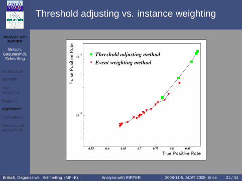
Threshold adjusting vs. instance weighting
10-3
10-2
0.55 0.6 0.65 0.7 0.75 0.8 0.85
Event weighting methodThreshold adjusting method
Britsch, Gagunashvili, Schmelling (MPI-K) Analysis with RIPPER 2008-11-5, ACAT 2008, Erice 21 / 34

Analysis withRIPPER
Britsch,Gagunashvili,
Schmelling
Introduction
RIPPER
cost-sensitivity
Bagging
Application
Comparison
Conclusionsand outlook
Different bagging parameters
10-3
0.4 0.5 0.6 0.7 0.8
bagging 3 iterationbagging 40 iterationbagging 25 iteration
Britsch, Gagunashvili, Schmelling (MPI-K) Analysis with RIPPER 2008-11-5, ACAT 2008, Erice 22 / 34

Analysis withRIPPER
Britsch,Gagunashvili,
Schmelling
Introduction
RIPPER
cost-sensitivity
Bagging
Application
Comparison
Conclusionsand outlook
Outline
1 Introduction
2 RIPPER
3 Cost-sensitive classification
4 Bagging
5 Applying the MVA algorithm
6 Comparison to other methods
7 Conclusions and outlook
Britsch, Gagunashvili, Schmelling (MPI-K) Analysis with RIPPER 2008-11-5, ACAT 2008, Erice 23 / 34

Analysis withRIPPER
Britsch,Gagunashvili,
Schmelling
Introduction
RIPPER
cost-sensitivity
Bagging
Application
Comparison
Conclusionsand outlook
Comparison with TMVA decision tree
TMVA [3] decisiontree(by Helge Voss):
boosting
pruning
10-3
10-2
0.55 0.6 0.65 0.7 0.75 0.8 0.85
WEKATMVA
false positive rate vs. true positive rate: TMVA tree, RIPPER
Britsch, Gagunashvili, Schmelling (MPI-K) Analysis with RIPPER 2008-11-5, ACAT 2008, Erice 24 / 34
Analysis withRIPPER
Britsch,Gagunashvili,
Schmelling
Introduction
RIPPER
cost-sensitivity
Bagging
Application
Comparison
Conclusionsand outlook
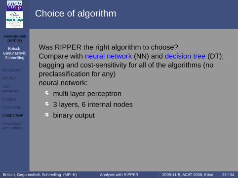
Choice of algorithm
Was RIPPER the right algorithm to choose?
Compare with neural network (NN) and decision tree (DT);bagging and cost-sensitivity for all of the algorithms (nopreclassification for any)neural network:
multi layer perceptron
3 layers, 6 internal nodes
binary output
decision tree
C 4.5
includes pruning
Britsch, Gagunashvili, Schmelling (MPI-K) Analysis with RIPPER 2008-11-5, ACAT 2008, Erice 25 / 34

Analysis withRIPPER
Britsch,Gagunashvili,
Schmelling
Introduction
RIPPER
cost-sensitivity
Bagging
Application
Comparison
Conclusionsand outlook
Choice of algorithm
Was RIPPER the right algorithm to choose?Compare with neural network (NN) and decision tree (DT);bagging and cost-sensitivity for all of the algorithms (nopreclassification for any)
neural network:
multi layer perceptron
3 layers, 6 internal nodes
binary output
decision tree
C 4.5
includes pruning
Britsch, Gagunashvili, Schmelling (MPI-K) Analysis with RIPPER 2008-11-5, ACAT 2008, Erice 25 / 34
Analysis withRIPPER
Britsch,Gagunashvili,
Schmelling
Introduction
RIPPER
cost-sensitivity
Bagging
Application
Comparison
Conclusionsand outlook
Choice of algorithm
Was RIPPER the right algorithm to choose?Compare with neural network (NN) and decision tree (DT);bagging and cost-sensitivity for all of the algorithms (nopreclassification for any)neural network:
multi layer perceptron
3 layers, 6 internal nodes
binary output
decision tree
C 4.5
includes pruning
Britsch, Gagunashvili, Schmelling (MPI-K) Analysis with RIPPER 2008-11-5, ACAT 2008, Erice 25 / 34

Analysis withRIPPER
Britsch,Gagunashvili,
Schmelling
Introduction
RIPPER
cost-sensitivity
Bagging
Application
Comparison
Conclusionsand outlook
Comp. with neural network and decision tree
10-3
0.4 0.5 0.6 0.7 0.8
Multilayer perceptron algorithmDecision tree algorithmRIPPER algorithm
false positive rate vs. true positive rate: NN, tree, RIPPER
Britsch, Gagunashvili, Schmelling (MPI-K) Analysis with RIPPER 2008-11-5, ACAT 2008, Erice 26 / 34

Analysis withRIPPER
Britsch,Gagunashvili,
Schmelling
Introduction
RIPPER
cost-sensitivity
Bagging
Application
Comparison
Conclusionsand outlook
Outline
1 Introduction
2 RIPPER
3 Cost-sensitive classification
4 Bagging
5 Applying the MVA algorithm
6 Comparison to other methods
7 Conclusions and outlook
Britsch, Gagunashvili, Schmelling (MPI-K) Analysis with RIPPER 2008-11-5, ACAT 2008, Erice 27 / 34

Analysis withRIPPER
Britsch,Gagunashvili,
Schmelling
Introduction
RIPPER
cost-sensitivity
Bagging
Application
Comparison
Conclusionsand outlook
Conclusions
Cost-sensitive, sampling and cutting on probability arevery similar
instance weighting better for some classifiers
bagging helps unstable classifiers, reduces overfitting
Analysis w/ RIPPER, bagging, instance weighting:
RIPPER fast and efficient to use
bagging and instance weighting very important
better than TMVA decision tree
RIPPER better than NN or DT
Britsch, Gagunashvili, Schmelling (MPI-K) Analysis with RIPPER 2008-11-5, ACAT 2008, Erice 28 / 34

Analysis withRIPPER
Britsch,Gagunashvili,
Schmelling
Introduction
RIPPER
cost-sensitivity
Bagging
Application
Comparison
Conclusionsand outlook
Outlook
use it for other analyzes (e.g. D0)
implement instance weighting in TMVA (and RIPPER?)
dependence on MC errors
increase weight on background in a more efficient way
Britsch, Gagunashvili, Schmelling (MPI-K) Analysis with RIPPER 2008-11-5, ACAT 2008, Erice 29 / 34

Analysis withRIPPER
Britsch,Gagunashvili,
Schmelling
Bibliography
Backup slides
Outline
8 Bibliography
9 Backup slides
Britsch, Gagunashvili, Schmelling (MPI-K) Analysis with RIPPER 2008-11-5, ACAT 2008, Erice 30 / 34

Analysis withRIPPER
Britsch,Gagunashvili,
Schmelling
Bibliography
Backup slides
W. W. Cohen, Fast Effective Rule Induction, In MachineLearning: Proc. of the 12th International Conference onMachine Learning, Lake Tahoe, California: MorganKaufman, 1995
http://www.cs.waikato.ac.nz/ml/weka/
TMVA Toolkit for multivariate data analysis with root, A.Höker et al., arXiv physiscs/0703039, http://tmva.sf.net.
Britsch, Gagunashvili, Schmelling (MPI-K) Analysis with RIPPER 2008-11-5, ACAT 2008, Erice 31 / 34

Analysis withRIPPER
Britsch,Gagunashvili,
Schmelling
Bibliography
Backup slides
Outline
8 Bibliography
9 Backup slides
Britsch, Gagunashvili, Schmelling (MPI-K) Analysis with RIPPER 2008-11-5, ACAT 2008, Erice 31 / 34
Analysis withRIPPER
Britsch,Gagunashvili,
Schmelling
Bibliography
Backup slides
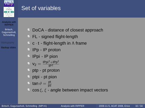
Set of variables
DoCA - distance of closest approach
FL - signed flight-length
c · t - flight-length in Λ frame
IPp - IP proton
IPpi - IP pion
v2 = IPpi2+IPp2
IP2
ptp - pt proton
ptpi - pt pion
tan ϑ = ptpz
cos ξ, ξ - angle between impact vectors
Britsch, Gagunashvili, Schmelling (MPI-K) Analysis with RIPPER 2008-11-5, ACAT 2008, Erice 32 / 34

Analysis withRIPPER
Britsch,Gagunashvili,
Schmelling
Bibliography
Backup slides
A new variable: ξ
p
π
ξ
PV
Λ
Britsch, Gagunashvili, Schmelling (MPI-K) Analysis with RIPPER 2008-11-5, ACAT 2008, Erice 33 / 34

Analysis withRIPPER
Britsch,Gagunashvili,
Schmelling
Bibliography
Backup slides
Imbalanced data sets in HEP and data mining
typical data mining applicationcredit card fraud, AIDS testrare class is "fraud transaction" or "AIDS infection"→ high cost not detecting rare instance
HEP mostly (particle selection)high backgroundhigh cost for (non-rare) background classified as signal
which translates to:data mining: imbalance has to be balancedHEP particle selection: imbalance has to be enhanced
Britsch, Gagunashvili, Schmelling (MPI-K) Analysis with RIPPER 2008-11-5, ACAT 2008, Erice 34 / 34