application of the hilbert transform to doppler radar ... of the hilbert transform to doppler radar...
TRANSCRIPT

AEDC-TR-88-3
Application of the Hilbert Transform to Doppler Radar Signals from
a Hypervelocity Gun
Robert W. Cayse
Calspan Corporation/AEDC Division
April 1988
Final Report for Period August 1, 1985 - July 31, 1986
Im~ "~i;UlIi~L LIBRAFI¥
Approved for public release; distribution is unlimited.
ARNOLD ENGINEERING DEVELOPMENT CENTER ARNOLD AIR FORCE STATION, TENNESSEE.
AIR FORCE SYSTEMS COMMAND UNITED STATES AIR FORCE

N O T I C E S
When U. S. Government drawings, specifications, or other data are used for any purpose other than
a definitely related Government procurement operation, the Government thereby incurs no responsibility
nor any obligation whatsoever, and the fact that the Government may have formulated, furnished, or
in any way supplied the said drawings, specifications, or other data, is not to be regarded by implication
or otherwise, or in any manner licensing the holder or any other person or corporation, or conveying
any rights or permission to manufacture, use, or sell any patented invention that may in any way be
related thereto.
Qualified users may obtain copies of this report from the Defense Technical Information Center.
References to named commercial products in this report are not to be considered in any sense as an
endorsement of the product by the United States Air Force or the Government.
This report has been reviewed by the Office of Public Affairs (PA) and is releasable to the National
Technical Information Service (NTIS). At NTIS, it will be available to the general public, including foreign
nations.
APPROVAL STATEMENT
This report has been reviewed and approved.
ROBERT W. SMITH Directorate of Technology Deputy for Operations
Approved for publication:
FOR THE COMMANDER
MARION L. LASTER Technical Director Directorate of Technology Deputy for Operations

UN CLASS I FI ED SECURITY CLASSIFICATION OF THIS PAGE
REPORT DOCUMENTAl'ION PAGE
la. REPORT SECURITY CLASSIFICATION UNCLASSIFIED
l 2a. SECURITY CLASSIFICATION AUTHORITY
2b. DECLASSIFICATION IDOWNGRADING SCHEDULE
4. PERFORMING ORGANIZATION REPORT NUMBER(S)
AEDC-TR-88-3
fro. NAME OF PERFORMING ORGANIZATION Arnold Engineering Development Center AOOReSS (oty, stete, ~ z ~ e c ~ Ai r Force Systems Command Arnold Air Force Base, TN
6b. OFFICE SYMBOL
DOT
37389-5000
8a. NAME OF FUNDING/SPONSORING 8b. OFFICE SYMBOL ORGANIZATION Arnold (ff ~op#ce~
En~ineertn~ Development Center DO k ADDRESS (C~, Stete, ~ ZW Cod,)
A i r Force Systems Command Arnold Air Force Base, TN 37389-5000
11. TITLE (Mc/ude Security Classification) Application of the Hi lber t Transform to Doppler
1 b. RESTRICTIVE MARKINGS
I rorm~oproved OMB No. 0704-0188
3 DISTRIBUTION/AVAILABILITY OF REPORT Approved for public release; d i s t r i bu t i on is unlimited.
S. MONITORING ORGANIZATION REPORT NUMBER(S)
7a. NAME OF MONITORING ORGANIZATION
7b. ADDRESS(CRy, State, and ZfPCode)
9 PROCUREMENT INSTRUMENT IDENTIFICATION NUMBER
10. SOURCE OF FUNDING NUMBERS PROGRAM PROJECT TASK WORK UNIT ELEMENT NO. NO. NO ACCESSION NO 65807F
Radar Signals from a Hypervelocity Gun
12.PEI~ONALAJJTHOR(.~) uayse, Konert w., Calspan Corporation, AEDC .Division
13a. TYPEFinalOF REPORT I|13b'FROM 1D/]/86TIME COVERED TOG/2£/R7 J14. O~rlO ~ R ~ (Year, Month, Day) lB. PAG~OUNT
I§. SUPPLEMENTARY NOTATION
Available in Defense Technical Information Center (DTIC).
17. COSATI CODES 18. SUBJECT TERMS (Continue on reverse i f necessary and identify by block number)
FmELD GROUP SUBGROUP hypervelocity guns Fourier transform 17 09 radar signal s Hi 1bert transform 14 0 r . popoler radar sianals enn.~uter nrnnram~
19. ABSTRACT (Continue on reverse i f necessary and identify by block number)
A computer program is described that processes a Doppler radar signal to provide the posi t ion, ve loc i ty , and acceleration h is tor ies of a model in the barrel of a hyper- velocity gun. The program uses the Hilbert transform as obtained via the Fourier transform. Algorithms for dealing with poor signal quality are described. Results from actual and simulated signals are presented. I t is shown that the unique properties of the Hilbert transform result in a program that is fast, accurate, and easy to use.
20. DISTRIBUTION/AVAILABILITY OF ABSTRACT 21 ABSTRACT SECURITY CLASSIFICATION I--I UNCLASS|FIEDAJNLIMITED [ ] SAME AS RPT. I--I OT~C USERS UNCLASSIFIED |
22a. NAME OF RESPONSIBLE INDIVIDUAL 22b.TELEPHONE(/nc/ude AreaCode) 22c OFFICE SYMBOL C. L. Garner .(615) 454-7B1~ [~CS
DD Form 1473, JUN 86 PreWoused~omare obsolete. SECURITY CLASSIFICATION OF THiS PAGE
UNCLASSIFIED

AEDC-TR-88-3
PREFACE
The work reported herein was performed by the Arnold Engineering Development Center
(AEDC), Air Force Systems Command (AFSC) at the request of the Directorate of Technology
(DOT), AEDC. The DOT Project Manager was Robert W. Smith. The Calspan Project
Manager was William T. Strike. The results were obtained by Calspan Corporation, AEDC
Division, operating contractor of the aerospace flight dynamics testing efforts at the AEDC,
AFSC, Arnold Air Force Base, Tennessee. The research was performed in the yon K/trm~m Gas Dynamics Facility (VKF), during the period of October 1, 1986 through June 26, 1987,
under the AEDC Project Number DB95VW (Calspan Number V32C-CG). The manuscript
was submitted for publication March 7, 1988 and was originally prepared in partial completion
of the requirements for a Master's Degree at the University of Tennessee Space Institute,
TuUahoma, Tennessee.
The author wishes to extend special thanks to Dr. Bruce W. Bomar, for his encouragement,
suggestions, and criticism; to Dr. Julius Bendat, for providing the initial encouragement to
apply the Hilbert transform to radar signals; to the Engineering Appfications Section of OAO, Incorporated, for computer graphics support; and to Mr. Howard Harris, for providing
countless technical details about the Range G radar system and data.
AEDC-TR-88-3
CONTENTS
Page
1.0 INTRODUCTION ...................................................... 5
1.1 Background Informat ion ............................................. 5
1.2 Statement o f the Problem and Study Objective . . . . . . . . . . . . . . . . . . . . . . . . . 5
1.3 Approach .......................................................... 6
2.0 TEST FACILITY ....................................................... 6
2.1 Light /Gas Launcher ................................................. 6
2.2 Interior Ballistic Doppler Radar System ................................ 7
3.0 T H E O R E T I C A L DEVELOPMENT ....................................... 7
3.1 Doppler Radar ...................................................... 7
3.2 Previous Data Reduction Methods ..................................... 8
3.3 Hilbert Transform ................................................... 8
3.4 Comparison of Two Methods ......................................... l 1
3.5 Smoothing and Differentiation ........................................ I I
4.0 P R O G R A M DESCRIPTION ............................................. 12
4.1 Program Summary .................................................. 13
4.2 Calculating the Hilbert Transform ..................................... 13
4.3 Signal Filtering ...................................................... 14
4.4 Unwrapping the Phase Angle ......................................... 15
4.5 Hanning Smoothing ................................................. 15
4.6 Velocity ............................................................ 16
4.7 Posit ion and Acceleration ............................................ 17
4.8 Query Program ..................................................... 17
5.0 RESULTS .............................................................. 17
5.1 Simulated signals .................................................... 17 5.2 Range G Radar Signals .............................................. 18
5.3 Performance ........................................................ 19
5.4 Future Work ....................................................... 20
6.0 CONCLUSIONS AND RECOMMENDATIONS . . . . . . . . . . . . . . . . . . . . . . . . . . . . 20
6.0 REFERENCES ......................................................... 21
ILLUSTRATIONS
Figure Page
1. Hypervelocity Range/Track (G) ........................................... 23
2. Range G Launcher ...................................................... 24

AEDC-TR-88-3
Figure Page
3. Doppler Radar in the Gun Barrel ......................................... 25
4. Analytic Signal ......................................................... 26
5. Analytic Signal and Peak-Picking Methods ................................. 27
6. Low-Pass Nature of Harming Window ..................................... 28
7. Box Car Filter .......................................................... 28
8. Phase Angle Unwrapping ................................................ 29
9. Typical End Effect of Smoothing Routine .................................. 30
10. Effect of Hanning Smoothing on Square Pulse . . . . . . . . . . . . . . . . . . . . . . . . . . . . . 31
11. Signal Amplitude Drop .................................................. 32
12. Velocity Correction Algorithm ............................................ 33
13. Effectiveness of Velocity Correction Algorithm . . . . . . . . . . . . . . . . . . . . . . . . . . . . . 34
14. Theoretical Trajectory for Simulated Signals ............................... 35
15. TXHARS Results with Perfect 3.6-GHz Signal . . . . . . . . . . . . . . . . . . . . . . . . . . . . . 36
16. TXHARS Results with Perfect 24-GHz Signal ............................... 37
17. Effect of Noise on Simulated 3.6-GHz Results . . . . . . . . . . . . . . . . . . . . . . . . . . . . . . 38
18. Effect of Noise on Simulated 24-GHz Results . . . . . . . . . . . . . . . . . . . . . . . . . . . . . . 40
19. Typical 3.6-GHz Results ................................................. 43
20. Typical 24-GHz Results .................................................. 44
21. Adverse Helix Offset Caused by Amplitude Drop . . . . . . . . . . . . . . . . . . . . . . . . . . . 45
22. Effect of Signal Length on Processing Time ................................ 46
APPENDIX
A. Query Program Parameters and Operation ................................. 47
NOMENCLATURE ..................................................... 48
4

AEDC-TR-88-3
1.0 INTRODUCTION
1.1 BACKGROUND INFORMATION
A vehicle encounters tremendous heating loads during atmospheric reentry. In order to survive, it must have an effective heat shield. Because flight testing is very expensive, candidate heat shield mateials are often screened through ground testing.
One such ground testing technique used at the Arnold Engineering Development Center (AEDC) is to attach a small specimen of candidate heat shield material onto a support body and launch the model into a controlled atmosphere at hypervelocity. This procedure is often used in the yon K~rm{m Gas Dynamics Facility (VKF) Hypervelocity Range/Track ((3).
A model is accelerated to hypervelocity in a short distance and, thus, encounters high axial accelerations, often in excess of I00,000 g. A one-dimensional (l-D) gas dynamics code predicts that the problem of high-g loading is further compounded when shock waves in the launching gas reflect from the aft end of the model and cause acceleration peaks. It has been hypothesized that these peak accelerations have caused material sample failures during some launches. (More recently, the high accelerations of launch have been exploited for survivability testing of small electronic packages.)
For test planning purposes, the I-D gas dynamics model is used to predict the velocity of models launched in Range G. In order to validate the accuracy of the prediction program, it is desirable to know the actual velocity and acceleration histories of models while they are still in the gun barrel. Thus, a Doppler radar system has been installed in Range G in order to (1) aid validation of the launcher performance prediction program, (2) assist investigations of material sample failures, and (3) measure the accelerations imparted to electronics packages.
The Doppler radar system produces a signal with a frequency proportional to the model velocity. Previous attempts to calculate acceleration from recorded radar signals have included manually measuring the time intervals between signal peaks and zero crossings. Because the peak interval measurements are labor intensive, and because the calculated results are adversely affected by even small errors in the interval measurements, these methods have achieved only limited success. Thus, an alternate method of obtaining the model acceleration from the radar signal was sought.
1.2 STATEMENT OF THE PROBLEM AND STUDY OBJECTIVE
The acceleration histories of models launched in Range G must be measured to validate launcher performance prediction methods and to aid investigations of material specimen failures. The objective of this study was to develop and verify a computer program for accurately and efficiently calculating model accelerations from Doppler radar data.

AEDC-TR-88-3
1.3 APPROACH
A literature search was conducted in order to find a better method of calculating the instantaneous model accelerations. The search revealed that the Hilbert transform was well- suited for the job because it can be used to obtain the instantaneous frequency of a signal and because it can be easily calculated using the fast Fourier transform (FFT). For the case of the Range G Doppler radar signal, the instantaneous frequency is directly proportional to the model velocity. It was then determined that a computer program could be developed that would obtain the model velocity from the Doppler radar signal via the Hilbert transform and then numerically differentiate the velocity to obtain the model acceleration history.
The Doppler signal from a typical model launch contains tens of thousands of data points. It was found that the AEDC CRAY ® XMP/12 supercomputer had available an FFT subroutine suitable for processing such large arrays of data. The approach of the study was then to implement the Hilbert transform on the CRAY. A numerical differentiation algorithm was then added to form the basis of the radar data reduction program.
The program was applied to simulated radar signals. The results were compared to the known theoretical acceleration histories. Random noise was added to the simulated signals to determine the sensitivity of the program to imperfect signals. The program was then applied to data from several model launches, and the results from two radar systems were compared.
2.0 TEST FACILITY
The Hypervelocity Range/Track (G) shown in Fig. 1 is a test unit that is used for the measurement of the aerodynamic coefficients of models in hypervelocity free flight and for captive testing of material sample models along a track. The facility can be easily converted from the free-flight (range) configuration to the track configuration. The track configuration allows the recovery of models for posttest inspection. The facility consists of a launcher, a blast chamber, and the range/track.
2.1 LIGHT/GAS LAUNCHER
The Range G launcher (Fig. 2) is equipped with a 2.5-in. caliber, two-stage powder- hydrogen gun approximately 170 ft long. The launcher is a fourth-generation two-stage gun that has been in use since 1969 and has launched approximately 3,000 models at speeds up to 24,000 ft/sec.
The Munch cycle can be summarized as follows: Gun powder is ignited, which propels a piston along a pump tube. The piston compresses hydrogen gas in the pump tube. When
6

AEOC-TR-88-3
the hydrogen pressure becomes sufficiently high, a rupture disk breaks, which then allows the hydrogen to escape into the gun barrel. The high-pressure hydrogen then propels the
model out the barrel. Hydrogen is used because of its high speed of sound. The performance of the launch cycle is controlled by varying the amount of gun powder, the mass of the piston, the initial pressure of the hydrogen, the diaphragm rupture pressure, and the mass of the model.
2.2 INTERIOR BALLISTIC D O P P L E R R A D A R SYSTEM
The idea of using radar to measure the interior ballistics of guns is not new. Doppler radar, or microwave interferometry, was first used to measure projectile motions in guns as early as the 1950's (Refs. 1 and 2). At the AEDC, a microwave interferometer was used
in Range G in 1961 (Refs. 3 and 4).
The operation of the Range G radar system can be summarized as follows: A reflex ldystron
transmits microwave energy through an antenna that performs both the transmitting and receiving functions. The microwaves travel from the barrel exit toward the model. The microwave energy reflects from the front of the model and then returns to the antenna. The reflected microwaves are mixed with the transmitted microwaves resulting in an oscillating signal that is recorded on analog magnetic tape. Equipment for operation at either 3.6 or
24 GHz is available.
3.0 THEORETICAL DEVELOPMENT
3.1 D O P P L E R R A D A R
When electromagnetic waves are reflected from a moving object, the reflected waves undergo a Doppler shift (Ref. 5). When sensed by an antenna that is designed for sensing the constructive/destructive interference of the transmitted and reflected waves, the antenna produces a signal that undergoes cyclic changes as the object moves. For the case of a model in the Range O launcher, the signal will go through one complete cycle for every half- wavelength travelled by the model (Fig. 3). The Doppler frequency, f(t), is described by Eq. (l).
f(t) (I) = ~,
where i(t) is model velocity, X is the radar wavelength, and t is time.
It should be pointed out that the wavelength, X, is the wave guide wavelength, not the free-space wavelength. Two radar systems are considered in this report. For the 3.6-OHz system, X is 0.422 ft; and for the 24-GHz system, X is 0.0424 ft.
7

AEDC-TR-88-3
3.2 PREVIOUS DATA REDUCTION METHODS
Doppler radar has been in use for measuring the velocity of moving objects since the early 1940's when it was used to measure aircraft velocity (Ref. 6). For most applications, velocity is quasi-steady (i.e. low accelerations), and typically simple tracking filters are used.
However, in hypervelocity guns such as the Range G launcher, the velocity and Doppler frequency change drastically in just a few milliseconds. In order to get a valid acceleration history, the Doppler signal must be analyzed in detail for an extremely large range of
frequencies. Thus, past methods of analyzing Doppler radar signals from gun barrels have focused on measuring the duration of each cycle of the signal.
The current method used to reduce the Doppler radar data from the Range G launcher
is based on Eq. (1), which can be rearranged as
x(t) - )~f(t) (2) 2
If one defines the duration of the i th half-cycle of the signal as ATi, then Eq. (2) is
approximated by ),
xi -- ~ (3)
A computer graphics terminal is used so that an operator can position a cursor over each signal peak in order to measure the values of ATi for all the half-cycles of a model launch.
Hence, this technique is dubbed the "peak-picking" method. The velocity history of Eq.
(3) is then differentiated to obtain the model acceleration.
3.3 HILBERT TRANSFORM
The I-Iilbert transform was developed by the German mathematic.an David Hilbert (1862-1942). Since its development, the transform has seen only limited application; and in light of the popularity of the Fourier transform, the Hilbert transform can be considered obscure. It does possess some rather unique properties (Refs. 7 and 8) that have led to its use in some relatively diverse fields. Some recent examples include image enhancement (Ref. 9), structural dynamic damping measurements (Ref. 10), characterization of nonlinearities in structures (Ref. 11), and electronic communication (Refs. 12 and 13).
The Hilbert transform of an oscillating time-wise function, y(t), is a second function of time, ~(t), where

AEDC-TR-88-3
y ' ( t )= H[y(t)] = ~ ~ d u
If we create a complex analytic signal (Refs. 7 and 8),
z(t) = y(t) + j ~ t ) , j = X/X-i "
we can obtain some very useful properties as shown in the following text.
Any complex variable can be written in exponential form, so z(t) can be written as
where
and
z(t) = A(t)exp[j$(t)]
(4)
A(t) = [y2(t) + y'2(t)]l/2
(5)
~ ( t ) = Tan- l [ - ~ ]
(6)
(7)
(8)
Thus, z(t) is a helix in complex space with radius A(t) and phase angle ~(t) as shown in Fig. 4. A(t) is also the instantaneous amplitude of y(t) and of y'(t). The instantaneous frequency is given by
f(t) - ~(.t_) (9)
from which we can calculate velocity using Eq. (2). Thus, if the Hilbert transform of the Range G Doppler radar signal can be obtained, the model position, velocity, and acceleration histories can be easily calculated.
A method for obtaining the Hilbert transform of a signal via the Fourier transform and the analytic signal is presented in Ref. 8 and is shown here.
(lO)
The Fourier transform is defined as
Y(f) = F[y(t)] = I ® y(t)exp (-j2~-ft) dt
The convolution property of the Fourier transform gives
9

AEDC-TFI-88-3
F[yl(t) * y2(t)] = F[yl(t)]F[y2(t)]
= Yt(f)Y2(f)
where • denotes convolution, which is defined as
Yl(t ) * Y2(t) ---- I°~Yl(U)Y2(t -- U) du - - 0 0
(11)
(12)
Since the definition of the Hilbert transform [Eq. (4)] is equivalent to the convolution of y(t) and 1 / ~ ; i.e.,
1 ~(t) = y(t) • ~ (13)
We can use Eq. (11) to write
F[ ~(t)] = FlY(t) * I ] = F [y ( t ) ]F ( I )
where
= Y ( 0 [ - J • s g n ( 0 ]
- l , f < 0 sgn(f) = 1, f _> 0
The Fourier transform of the analytic signal [Eq. (5)] is
Z ( 0 = F[z(t)I = F[y(t)I + j F [ ~ ( t ) ]
Upon substituting Eq. (14), we obtain
Z(f) = Y(f ) + J Y ( 0 [ - J • sgn(O]
= Y(f)[1 + sgn(0] = B(f)Y(f)
(14)
(15)
(16)
(17)
( i s )
where
0, f < 0 B(f) = 2, f > _ 0
10

AEDC-TR-88-3
From inspection of Eqs. (17) and (18), we can see that, given the Fourier transform of y(t), we very easily obtain the Fourier transform of z(t) by setting Y(f) to zero for negative frequencies and by multiplying Y(f) by 2 for positive frequencies. The analytic signal can then be obtained via the inverse Fourier transform.
3.4 COMPARISON OF TWO METHODS
The primary advantage of the analytic signal method of calculating velocity over the peak- picking method is illustrated in Fig. 5. The analytic signal method provides a continuous estimate of the signal phase angle, whereas the peak-picking method provides a stair-step phase angle history. Thus, the differentiation needed to obtain the model velocity can be more readily performed using the continuous curve of the analytic signal method rather than the disjointed curve of the peak-picking method.
3.5 SMOOTHING AND DIFFERENTIATION
Numerical differentiation of a noisy function typicaUy magnifies the effect of the noise. If one can tolerate a loss-of-time resolution, numerical smoothing can be applied either before or after the differentiation to reduce the effect of the magnified noise. The Harming filter is a well-known smoothing technique and, as shown below, can be combined with the numerical differentiation into a single operation.
The normalized Hanning window, h(t), is defined as
h(t) =
10, t < - T
2 1( ¥ I - c o s m 2
0, t > T m
2
( 1 9 )
where T is the time span of the window. The low-pass nature of Hanning smoothing is illustrated in Fig. 6.
If x(t) is a function to be differentiated, and i(t) is the result of the differentiation, i(t) can be smoothed by convolution with the Hanning window yielding
11
AEDC-TR-88-3
x'(t) = h(t) • i ( t ) = I=h(u) i ( t - u) du - - O 0
Integration by parts gives
x '( t) = - h(u)x(t - u) + I ® l~(u)x(t - u) du
Substitution of Eq. (19) gives
i ' ( t ) = 0 +
T U ~
T U ~ m m
2
T 22-'~T sin ( - ~ ) x ( t - u) du
(2o)
(21)
(22)
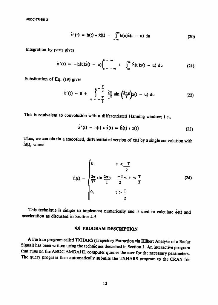
This is equivalent to convolution with a differentiated Hanning window; i.e.,
i ' ( t ) = h(t) • x(t) = l~(t) • x(t) (23)
Thus, we can obtain a smoothed, differentiated version of x(t) by a single convolution with ll(t), where
fi(t) =
f '0, t < - T
2
2~r sin 2_Tt, - T ~ t _< T (24)
0, t > T m
2
This technique is simple to implement numerically and is used to calculate ~(t) and acceleration as discussed in Section 4.5.
4.0 P R O G R A M DESCRIPTION
A Fortran program called TXHARS (Trajectory Extraction via Hilbert Analysis of a Radar Signal) has been written using the techniques described in Section 3. An interactive program that runs on the AEDC AMDAHL computer queries the user for the necessary parameters. The query program then automatically submits the TXHARS program to the CRAY for
12
AEDC-TR-88-3
execution. After TXHARS executes, the results are sent back to the AMDAHL where the
user can view the results using TEKPLOT, an interactive graphics program available at the
AEDC.
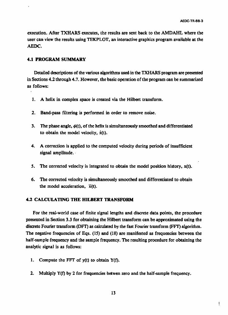
4.1 PROGRAM SUMMARY
Detailed descriptions of the various algorithms used in the TXHARS program are presented
in Sections 4.2 through 4.7. However, the basic operation of the program can be summarized
as follows:
1. A helix in complex space is created via the Hilbert transform.
2. Band-pass filtering is performed in order to remove noise.
3. The phase angle, ~(t), of the helix is simultaneously smoothed and differentiated
to obtain the model velocity, i(t).
4. A correction is applied to the computed velocity during periods of insufficient
signal amplitude.
5. The corrected velocity is integrated to obtain the model position history, x(t).
6. The corrected velocity is simultaneously smoothed and differentiated to obtain
the model acceleration, ~(t).
4.2 CALCULATING THE HILBERT TRANSFORM
For the real-world case of finite signal lengths and discrete data points, the procedure
presented in Section 3.3 for obtaining the Hilbert transform can be approximated using the
discrete Fourier transform (DFT) as calculated by the fast Fourier transform (FFT) algorithm.
The negative frequencies of Eqs. (15) and (18) are manifested as frequencies between the
half-sample frequency and the sample frequency. The resulting procedure for obtaining the
analytic signal is as follows:
1. Compute the FFT of y(t) to obtain Y(f).
2. Multiply Y(f) by 2 for frequencies betwen zero and the half-sample frequency.
13

AEDC-TR-88-3
3. Set Y(f) to zero for frequencies between the half-sample frequency and the sample frequency. [Steps 2 and 3 yield Z(f).]
4. Compute the inverse FFT of Z(f) to obtain z(t).
The TXHARS program uses the IMSL subroutine FFTCC (Ref. 14) to compute the FFT of the radar signal and the inverse FFT of the analytic signal to obtain the Hilbert transform of the radar signal. Since the subroutine does not have a constraint on the number of data points, the very large array defining the radar signal can be processed with only one call for the FFT and a second call for the inverse FFT. This is simpler and more efficient than segmenting the signal into several short pieces and making several calls to the FFT subroutine. To date, radar signals containing up to 40,000 data points have been processed.
4.3 SIGNAL FILTERING
Since the signals from the radar system are typically noisy, provisions for filtering the radar signal are included in TXHARS. Since signal frequency is proportional to model velocity, any signal content at frequencies higher than that of the maximum velocity achieved by the model can be assumed to be noise. Also, very-low-frequency data (such as signal drift) can
also be ignored since the model achieves a finite velocity in a very short time when hit by the first hydrogen pulse. Thus, the program user is allowed to select a velcoity range of interest that is defined by VMIN and VMAX. Signal frequencies corresponding to velocities outside the range of interest are eliminated by band-pass filtering.
The band-pass f'fltering is performed in the frequency domain by zeroing out Z(f) at frequencies outside the band-pass limits fl and f2. This results in a simple "box car" filter as illustrated in Fig. 7. The band-pass limits are calculated by
fl = 0.9 (2 . VMIN), f2 = l.l (2 • VMAX) (25)
The factors outside of the parentheses serve to slightly broaden the pass band.
One shortcoming of the box car filter is the phenomenon known as "ripple" (Ref. 15), which is illustrated as the scalloped curve in Fig. 7. Ripple is the result of approximating
a continuous spectrum with discrete points. This causes nonzero filter components to exist within the stop bands and nonunity components to exist in the pass band. A more advanced filter that has less ripple than the box car could have been used, but the box car is very easy to implement and has provided acceptable results to date.
14

AEDC-TR-88-3
After the box car filter is applied to Z(0, we are left with Z ' (0. The inverse FFT of Z ' (f) then gives
z '( t) = y ' ( t ) + j ~ ' (t) (26)
where y '( t) is the filtered radar signal, and y'(t) is the Hilbert transform of y'(t) .
4.4 UNWRAPPING THE PHASE ANGLE
The amplitude, A(t), and phase angle, ~k(t), of the filtered signal are calculated using Eqs.
(7) and (8). However, since the inverse tangent function available in Fortran only provides
results ranging from - a- to + r , the O(t) values must be "unwrapped" as illustrated in Fig. 8. The program has an unwrapping algorithm that appropriately adds or subtracts 2a- from
the phase angle whenever two consecutive points are in the second and third quadrants.
4.$ HANNING SMOOTHING
TXHARS uses the Hanning window methods presented in Section 3.5 to smooth the velocity, acceleration, and signal amplitude histories. A window that covers a large time span is effective at removing unwanted noise from the results, but it also removes desired detail.
Conversely, a window that covers a small time span provides better detail, but can also pass too much noise. Thus, the program was designed so that the user can adjust the time span
of the windows in order to reach an acceptable compromise between noise and detail.
Since each of the data arrays to be smoothed is of finite length, the Hanning window cannot function properly at the array ends. This is because there are no data points available
for convolution with the Hanning window outside of an array. Therefore, for these periods the program uses the convolution value obtained at the most extreme point for which full overlap occurs. This results in a small flat at each end of a smoothed array. This effect is illustrated in Fig. 9.
Figure 10 shows the effect of Hanning windows of various time spans on a rectangular pulse. The figure is presented in dimensionless form. The pulse begins at time zero, immediately
obtains a value of one, and then drops back to zero at time one. The R = 0.5 curve shows
that a very good approximation of a pulse is obtained when a rectangular pulse is smoothed
by a Hanning window with a time width one-half the pulse width. A very poor approximation is obtained when the Hanning width is 10 times the pulse width as shown by the R = 10 curve.
As an example, suppose one wanted to know the peak g loading encountered during acceleration pulses lasting more than 0.1 msec. The R = 1 curve of Fig. 10 shows these peak
15

AEDC-TR-88-3
values could be obtained with a Harming window as large as 0.1 msec. Note that the detailed
shape of the acceleration curve would be incorrect.
It should also be pointed out that the response curves of Fig. 10 apply to the difference
between the pulse height and the nominal value, not the absolute height. As another example,
suppose the nominal acceleration of the model was 100,000 g, then suddenly jumped to 150,000
g for 0.1 msec. The R = 2 curve shows that a Hanning window of a 0.2-msec span would
obtain the 100,000-g nominal acceleration plus about 84 percent of the 50,000-g difference.
Thus, the TXHARS output for the peak acceleration would be 142,000 g. This would be
considered a reasonable engineering estimate of peak acceleration since it respresents an error
of only 5 percent.
Hanning windows with time widths greater than the pulse width of interest will always
underestimate the peak acceleration value, whereas signal noise typically causes the program
to overestimate the peak values. Knowledge of the Harming window widths and the signal
quality are, therefore, useful when interpreting the program output.
4.6 VELOCITY
An initial estimate of the model velocity, k(t), is found by first applying Eq. (24) to
simultaneously smooth and differentiate ~(t) to get &(t); then Eqs. (9) and (2) are used to
get i(t). The velocity, i(t), must then be corrected because the amplitude of Range G radar
signals often drops to zero. Typical drops in amplitude are shown in Fig. 11 and are believed
to be caused by several phenomena that include antenna vibration and extraneous radar
reflections. Since these amplitude drops can significantly degrade the program results,
provisions are included in TXHARS to interpolate the velocity across these time periods.
This effectively "skips" the "bad" portions of the signal. The skipping algorithm uses a
floating criterion for identifying bad periods.
The floating criterion used in the ratio of a lightly smoothed trace of the signal amplitude,
A(t), with a heavily smoothed trace. Equation (19) is convolved with the data to perform
the smoothing. When the lightly smoothed curve is less than a user-specified fraction of the
heavily smoothed curve, velocity interpolation is performed. After interpolation is performed,
Eq. (19) is convolved with i(t) in order to eliminate kinks in the curve. The algorithm is
illustrated in Fig. 12. The effect of turning off the skipping algorithm is shown in Fig. 13.
Note the large spikes on the "Without Velocity Correction" velocity curve. These spikes
correspond to signal amplitude dropouts.
16
I
i
I

AEDC-TR-88-3
4.7 POSITION AND ACCELERATION
After the skipping algorithm processes the velocity history, i(t), the position, x(t), is calculated by numerically integrating velocity. A simple rectangular integration method is used. Acceleration, ~(t), is calculated by convolving the differentiated Hanning window of Eq. (24) with x(t).
4.8 QUERY PROGRAM
Because several parameters can be adjusted by the program user, an interactive query program has been added to TXHARS by the Engineering Applications Section of OAO, Incorporated, the computer services subcontractor at the AEDC. A typical session is presented in Appendix A along with definitions for the input variables. The query program was designed so that the user can easily track the variables used to produce the results of numerous launches and analyses. The query program automatically produces a hardcopy of the terminal screen at the end of each session. The session date and time are included on the hardcopy and stored for subsequent labeling of the plotted results.
5.0 RESULTS
$.1 SIMULATED SIGNALS
Several simulated signals have been generated in order to validate the TXHARS computer program. The acceleration histories produced by TXHARS were compared to the theoretical accelerations corresponding to each of the simulated signals. Figure 14 shows the theoretical model trajectory for one such simulation. Figure 15 shows the velocity and acceleration histories calculated by TXHARS for a simulated signal with a Doppler wavelength of the 3.6-GHz radar system, and Fig. 16 shows the trajectory calculated for a simulated 24-GHz signal. The close agreement of the calculated trajectories in Figs. 15 and 16 with the theoretical trajectory of Fig. 14 validates the basic operation of the program.
It can be seen that the acceleration curves of the simulated signals are oscillatory in nature. The period of the oscillation was selected to correspond to a duration of acceleration peak of 0.08 msec. This duration is typical of the acceleration pulses predicted by the launcher performance program.
It can be seen from Figs. 14 and 15 that both the 3.6- and 24-GHz signals could be used to resolve these peaks reasonably well. Acceleration peaks of shorter duration (i.e. higher frequency oscillations of the theoretical acceleration) could not be resolved nearly as well, with the results tending to be worse at the lower theoretical model velocities, especially for
17
I I
AEDC-TR-88-3
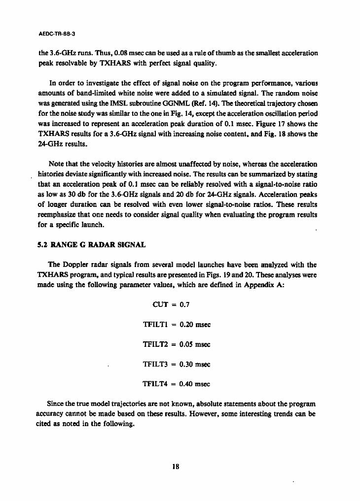
the 3.6-GHz runs. Thus, 0.08 msec can be used as a rule of thumb as the smallest acceleration
peak resolvable by TXHARS with perfect signal quality.
In order to investigate the effect of signal noise on the program performance, various
amounts of band-limited white noise were added to a simulated signal. The random noise
was generated using the IMSL subroutine GGNML (Ref. 14). The theoretical trajectory chosen
for the noise study was similar to the one in Fig. 14, except the acceleration oscillation period
was increased to represent an acceleration peak duration of 0.1 msec. Figure 17 shows the
TXHARS results for a 3.6-GHz signal with increasing noise content, and Fig. 18 shows the
24-GHz results.
Note that the velocity histories are almost unaffected by noise, whereas the acceleration
histories deviate significantly with increased noise. The results can be summarized by stating
that an acceleration peak of 0.1 msec can be reliably resolved with a signal-to-noise ratio
as low as 30 db for the 3.6-GHz signals and 20 db for 24-GHz signals. Acceleration peaks
of longer duration can be resolved with even lower signal-to-noise ratios. These results
reemphasize that one needs to consider signal quality when evaluating the program results
for a specific launch. i
5.2 RANGE G RADAR SIGNAL
The Doppler radar signals from several model launches have been analyzed with the
TXHARS program, and typical results are presented in Figs. 19 and 20. These analyses were
made using the following parameter values, which are defined in Appendix A:
CUT = 0.7
TFILTI = 0.20 msec
TFILT2 = 0.05 msec
TFILT3 = 0.30 msec
"ITILT4 = 0.40 msec
Since the true model trajectories are not known, absolute statements about the program
accuracy cannot be made based on these results. However, some interesting trends can be
cited as noted in the following.
18

AEDC-TR-88-3
As mentioned in Section 4.6, the amplitude of the radar signal occasionally drops to near zero. Theoretically, this should not pose a problem since the phase angle of the analytic signal should continue to increase during these periods. However, Fig. 21 shows that for actual data, the helix of the analytic signal typically is not centered around the time axis during the signal amplitude drop. This offset can be attributed to low-frequency noise in the signal. The offset causes the phase angle to oscillate, instead of increase, with time. The velocity correction algorithm described in Section 4.6 has proven to be successful in eliminating the adverse effects of the amplitude drop, but an improved filtering method might provide better results. Such a method would have to eliminate the helix offset of the amplitude drops without filtering out the low-frequency Doppler signal that occurs during the early period of a model
launch.
It is believed that one measure of signal quality is the size of the Hanuing windows used for smoothing the data. Typically, when a launch signal is analyzed for the first time, very small Harming windows are selected, and usually very noisy and unrealistic results are produced. The program is then reexecuted with increasing window widths until the program results are judged to be reasonable. (Usually no more than three or four runs are needed to get acceptable results.)
Signals from the 3.6-GHz system often require smaller windows and, thus, are felt to produce better results than the 24-GHz system. This would seem to be contrary to the results of the simulated signal study of Section 5.1 that indicate that the higher 24-GHz system should provide better results. However, experience has shown that the 24-GHz system produces much noisier signals than the 3.6-GHz system and that the amplitude of the signal from the 3.6-GHz system is less prone to drop to zero. In practice, therefore, the inferior signal quality of the 24-GHz system usually negates any inherent advantage it has over the 3.6-GHz system.
5.3 PERFORMANCE
Signals of various length have been analyzed with TXHARS, the largest containing 40,000 data points. Figure 22 shows the adverse effect of signal length on run time. However, the maximum central-processor time of 20 sec is considered to be a small job for the AEDC CRAY. The ellapsed time from job submittal to plotted results was typically 15 min and was largely unaffected by signal length.
Since the computation time of the FFT is proportional to N • log(N) (Ref. 14), where N is the signal length, we can conclude from the linearity of Fig. 22 that the run time of TXHARS is not significantly influenced by the FFT calculation. This suggests that data input and output are the major contributors to run time. Improved file handling methods might serve to make the program even more efficient.
19

AEDC-TR-88-3
5.4 FUTURE WORK
An effort is currently underway at the AEDC to acquire data simultaneously with both the 3.6- and 24-GHz systems. Also, these data will be analyzed using both the TXHARS program and the peak-picking methods. The results of this study should help reveal the strengths and weaknesses of the different systems and methods. New methods will also be introduced in an attempt to increase radar signal quality.
A new data acquisition system is currently being implemented in the Range G facility. This data system will have the capability to directly digitize the signal from the interior ballistics radar system as a model is launched. Thus, the need for magnetic tape will be eliminated. Since the internal memory capacity of the data acquisition system computer is several times larger than needed to hold the radar signal history from a typical launch, it may be feasible to run the TXHARS program on the new computer. This would be desirable since it would eliminate the data f'fle transfers presently required to move Range G radar signals to the CRAY. TXHARS could then provide results more promptly if it operated on the new data acquisition system computer.
In order to implement TXHARS on the new data acquisition computer, two obstacles must be overcome. First, an alternate method of calculating the Hilbert transform would have to be used since a suitable FFT routine is not available on this computer [One alternative is a finite-impulse-response digital filter (Ref. 15).] Second, TXHARS would have to be modified to operate with the plotting software available on the new computer, and it is not certain if the plotting software is suitable. Thus, further investigation is needed to determine if it is warranted to convert TXHARS for use on the new data acquisition system computer.
6.0 CONCLUSIONS AND RECOMMENDATIONS
The objective of this study was met by developing a data reduction program for the Range G interior ballistics radar system. The Hilbert transform has been shown to be well-suited for extracting model ballistic information from Doppler radar signals. The program has been shown to be accurate and efficient. Signals from the 3.6-GI-Iz system have proved to provide better results than those from the 24-GHz system.
It is recommended that the use of more advanced filtering methods be pursued in order to improve the ability of the program to deal with noisy signals. Data acquired simultaneously with both the 3.6- and 24-GHz systems should be evaluated, efforts to improve the quality of the radar signals from future tests in Range G should be continued, and the feasibility of implementing TXHARS on the new data acquisition system computer should be studied further.
20

AEDC-TR-88-3
REFERENCES
1. Yagi, F. et al. "Analysis of Interferometer Records of Projectile Motion in the Bore of Small Arms." Ballistic Research Lab., BRLR 939, May 1955.
2. Pennelegion, L. "Instrumentation of the University of Southampton Hypersonic Gun Tunnel." Doctorate Dissertation, University of Southampton, England, 1956.
3. Hendrix, R. E. "Microwave Measurement of Projectile Kinematics within Launcher Barrels." AEDC-TDR-62-213 (AD-288923), November 1962.
4. Hendrix, R. E. "Microwave Measurement of Projectile Kinematics within Launcher Barrels." M. S. Thesis, University of Tennessee, August 1963.
5. Cook, C. E. and Bernfeld, M. Radar Signals: an Introduction to Theory and Application. New York, Academic Press, 1967.
6. Ridenour, L. N., ed. Radar System Engineering. New York, McGraw-Hill Book Co., 1947.
7. Bracewell, R. N. The Fourier Transform and Its Applications. 2nd Edition. New York, McGraw-Hill Book Co., 1978.
8. Bendat, J. S. and Piersol, A. G. Random Data: Analysis and Measurement Procedures. Second Edition, John Wiley and Sons, 1986.
9. Belvaux, Y. and Vareille, J. C. "Visualization of Phase Objects by Hilbert Transform."NASA-TT-F- 14046, 1971.
10. Coppolino, R. N. "Integrated Dynamic Test/Analysis Processor Overview." MacNeal- Schwendler Corporation.
11. Coppolino, R. N., Bendat, J. S., and Stroud, R. C. "New Processor Integrates Dynamic Testing and Analysis." Sound and Vibration, August 1986, pp. 16-22.
12. Udalov, S. "Independent Sideband Modulation/Demodulation Using Digitally Implemented Hilbert Transforms." National Telesystems Conference, Galveston, Texas, Conference Record (184-15623 04-32), November 1982.
13. Henderson, R. G. and Lafrance, P. "Application of Digital Signal Processing to a Low Data Rate Communications Receiver." AIAA Paper No. 84-2652, 1984.
21

AEDC-TR-88-3
14. IMSL Library Reference Manual, Vol. 1, 9th Edition, IMSL, Inc., 1982.
15. Rabiner, L. R. and Gold, B. Theory and Application of Digital Signal Processing. New
Jersey, Prentice-Hall, 1975.
22

.... ~ '~'i ~ i~ii~i~ , ~
~i';¢ .....
~;~c ~ ~ ~ : .
i .......
Figure 1. Hypervelocity Range/Track (G).
:t~ ~ !~3~iy~',~ ~!~i~ s~- ,x~ ~ / ~ , c . . . . . . . . . . . . . .
~!ii!~/'̧ ~ ,
/ }
3* m O
-n i
c o i
60

m
i
i
Figure 2. Range G launcher.

AEDC-TR-88-3
Antenna Output
I I I
Figure 3. Doppler radar in the gun barrel.
"owave -gy
~ A n t e n n a
25

A E D C - T R - 8 8 - 3
J +(t)
-11" -I
l i//i / I i / /
i V
I t
+(t)
~(t
A(t)
i r !
!
. . .
t
Figure 4. Analytic signal.
26

A E D C - T R - 8 8 - 3
i l
I I I I
13 Signal Peaks
I i Time, t
16v
¢/t e - e~
L
V
0 1 e -
e - O=
14.
12.
lOw
8v
6~
4.
2=
0
A
4 J V
l=,==
¢...
o i =Ip~
! I l !
Phase Angle via Analytic Signal
Phase Angle via Peak Picking
Time, t
Figure 5. Analytic signal and peak-picking methods.
27

A E D C - T R - 8 8 - 3
1.0 (D
0 liT 21T Frequency
Figure6. Low-passnatureofHanning window.
31T
1.0
CU
4.)
Not to Scale
~ 1 ~ • Discrete Points
m
Used by FFT -------Resulting Continuous
Filter Effectiveness
f l f2 1 Sample Rate Frequency
Figure 7. Box car filter.
28

AEDC-TR-88 -3
A
V
c
V
I I I Time, t
14~ l I I I B m
10~- ..--I-" k - Unwrapped _ i / -
8~ - Phase Angle--~ / / / i I ~ . -
• 0 - 611" - - . . . " "
4~ I- / s Original I < ~ . , / / " Phase Angl e-.~
0
-2~ Time, t
Figure 8. Phase angle unwrapping .
29

AEDC-TR-88-3
Unsmoot
I Hann 1 ng
!
I I I m~½~j Smoothed Data I I L j "Flat"
t
Figure 9. Typical end effect of smoothing routine.
30

AEDC-TR-88-3
1.0
,,C
~.o .5
vI c- O
I X
R = I R=0.5
I
2
~R = 2
I R = Hannin9 Width ] Pulse Width I
/ 0 0 2 0 2 -4 -2 0 2 4
Time, pulse widths
Figure 10. Effect of Hanning smoothing on square pulse.
31

A E D C - T R - 8 8 - 3
4J V
>~
e - 0 1
¢/1
93.0 93.2 93.4 93.6 93.8
Figure 11. Signal amplitude drop.
94.0
32

r - - r~
= . 0
" 0 OJ %. OJ 4-I
.p- m.
-200'
15,000
U ,0J
,,Ik,t %-
4 J v o R
O
8,0001 15,000
I ! I I
(J OJ &n
%-
m
. lJ v . X
m
0
8,000 74.5
"Bad"
y'{t)
I .... I U!l Step I - Bad
Identi fled
~ ~!fJ~l,~IVi Amp'itude lil,llllli
J_J T 1 F
Corrected T -- V e l o c i t y ~ ..
jr "~ i ~ Un.corr.ected \ ~ / Velocity
l I I I
Step 2 - Linear Interpolation Performed Across Bad Period
- Smoothed, Corrected
A E D C - T R - 8 8 - 3
q
J I J 75.0
Time, t , msec
Figure 12. Velocity correction algorithm.
Step 3 - Corrected V e l o c i t y ' I s Smoothed
33

A E D C - T R - 8 8 - 3
I0,000
u
u~
.1~ q -
- X
t ~ u 0
@J
Without Velocity Correction
0 L 90
Time, t, msec 100
i0,000
U
of)
W-
A
V °X
u 0
With Velocity Correction
0 90
Time, t , msec
Figure 13. Effectiveness of velocity correction algorithm.
I00
34

, A E D C - T R - 8 8 - 3
u 0.1 (/1
4J q..
.-t" V
, X
i i ,m u O
20,000
0 0 5.0
Ti me, t, msec
160,000
V
: X
=- o
*lml
%. ~J
O u
I I I I
0 0 5.0
Time, t , msec
Figure 14. Theoretical trajectory for simulated signals,
35

AEDC-TR-88-3
20,000
U
¢J2,
4~ q -
.IV V
° X
U 0
p. . . .
Q,3
0 0 5.0
Time, t, msec
: X
0
L
u U
160,000
0 5•0 Time, t, msec
Figure 15. TXHARS results with perfect 3•6-GHz signal•
36

' A E D C - T R - 8 8 - 3
20,000
(.}
t/t
4-~ 4-
4~ V ,X
u 0
0
Time, t , msec 5 . 0
u~
.C 4J
V ; X
0 q . n
4-~ m S.
U U
160,000 I I I I
0 I I I I 0
Time, t , msec
Figure 16. TXHARS results with perfect 24-GHz signal.
t 5 . 0
37

A E D C - T R - 8 8 - 3
{.)
iF.
4.1 v °X
0
20,000
0
Signal-to-Noise Ratio, db: I ~-2-- Signal Amplitude '
20"I°gi0 2 • Noise Standard Deviation
0 Time, t, msec
5.0
160,000
4-=
; X
O
4-t tO s - a)
p . . .
a~ U U .:C
0 0 5.0
Time, t, msec : a. 40-db signal-to-noise ratio
Figure 1"/. Effect of noise on simulated 3.6-GHz results.
38

A E D C - T R - 8 8 - 3
20,000
r j 0J vJ
4,J q -
A 4-)
V . X
* t ' - - u O
.G,I
160,000
o'J
4J}
: X
0
L
U U
0
i I I i
0 0 5.0
Time, t, msec
0 5.0 Time, t , msec
b. 30-db signal-to-noise ratio Figure 17. Concluded.
39

A E D C - T R - 8 8 - 3
20,000
{J
&f)
a~ V
0X
U 0
I I I I
0 Time, t , msec
5.0
160,000
V ~x
o BIr'D
f,...
u u
I i I I
I J I I
Time, t , msec
a. 30-db signal-to-noise ratio Figure 18. Effect of noise on simulated 24-GHz results.
5 . 0
40

AEDC-TR-88-3
20,000
u CP
W-
v
,X
, r - -
0
QJ
0 Time, t , msec
5.0
160,000
4,.) V " X
O
S- ~D
u u
0 0
Time, t, msec
b. 2O-db signal-to-noise ratio Figure 18. Continued.
5.0
41

A E D C - T R - 8 8 - 3
20,000
u
4/I
4J 14..
4~ V
. X
o r~ u 0
I ' - - a,}
0 K; 0
Time, t, msec 5.0
160,0C ̂
c a
A
4 J V : X
0
4 J
l -
r . . .
u ( J
0 Time, t, msec
e. l$-db signal-to-noise ratio Figure 18. Concluded.
5 .0
42

A E D C - T R - 8 8 - 3
20,000
U ~J
q-
V
° X
4.a
U 0 m
m
0 70
I I I I
75 Time, t , msec
160,000
A
-'X
0 i i , m
e.._
u u
m
0 70
I I I
l I I I Time, t , msec
Figure 19. Typical 3.6-GHz results.
75
43

AEDC-TR-88-3
20 ,000 l
,X
0 76
m m
u
I I I 81
Time, t , msec i
160,000 l i I I
-*X
I p
u u
0 76 81
Time, t , msec
Figure 20. Typical 24-GHz results.
44

AEDC-TR-88-3
--W
t Phase Angle Oscillation
)(t)
Offset
y{t)
Figure 21. Adverse helix offset caused by amplitude drop.
45

AEDC-TR-88-3
20
16
u 12 UZ
E F- e , , ,
8
4
01
0 10 20 30
Signal Length, Thousands of Points
Figure 22. Effect of ~gn~ length on processing time.
40
46

N
LAMBDA
CUT
TFILTI
TFILT2
TFILT3
TFILT4
VMIN
VMAX
TSTART
AEDC-TR-88-'3
APPENDIX A QUERY PROGRAM PARAMETERS AND OPERATION
The program user will be prompted for the following variables:
The number of data points to be included in the analysis. Typically, numerous data points before and after the actual launch are recorded and stored on the computer. The user should select only those points that include the model launch.
The effective radar wavelength (in feet) in the barrel.
The ratio of the lightly smoothed to heavily smoothed amplitude histories used by the skipping algorithm for establishing a bad time period. Velocity interpolation across bad periods is performed. A value of zero for CUT turns
off the skipping algorthim.
The time span (in milliseconds) of the differentiated Hanning window used for
computing the uncorrected velocity history.
The time span (in milliseconds) of the Hanning window used for the lightly smoothed amplitude trace. The skipping algorithm multiplies this number by 7 to obtain the size of the Hanning window for computing the heavily smoothed
amplitude trace.
The time span (in milliseconds) of the Harming window used for smoothing the "corrected" velocity history produced by the skipping algorithm.
I
The time span (in milliseconds) of the differentiated Hanning window used for
computing the acceleration history.
The minimum velocity (in feet/second) of interest. Used for establishing the lower
pass-band frequency for filtering of the radar signal.
The maximum velocity (in feet/second) of interest. Used for establishing the upper pass-band frequency for filtering of the radar signal.
Time (in milliseconds) of the first point of the stored data to be included in the
analysis.
47

AEDC-TR-88-3
JPtL 10, 1987
Sample 1. Typical Query Session | o | X P.H,
[~?[R 38000 k
NUR|ER 0P P0|HYI IN I | | . ( N F i U , T • 4 N i l )
• a t l m l
k'flYER R4~WIMQEUNGTI4 IN F [ [ ? , 0.04~t34 LMe|IM • 0.04m
(DI~IIULT * 0 . 0 4 )
I[NTEII FIMCTION FOR FLONTXM CNZTI[IIOfl FOR UKLOCXTY CONIIECTION. CDEFAULT * O .? )
CUT • O.?O0
ENTER SIZE OF J4WlNIM UXHNU CflILL|KC) FOil tS? UI[L0CZTY .1 .gFILT$ • O. tel)
¢At,(XJli,~IT][Oel (DEF4ULI' • 0 , 0 3 )
[Hl'[It S I K OF J4WlNlJm iZNSOI I R I L L t K ¢ ) FM fSqPLITUB[ SIIOOTI4|HQ .1 lYILTR • • . 100
(I)I[FNIJLT ,, 0.03)
[ ~ B SIZ[ OF l l l INZN V|NI0 i CflILLZEC) WON UI[LOCITY SROOTIeZM .1 I'FXLT3 - O.100
(KFNULT • 0 . 0 3 )
i[NTI[N SIZE OF J~NNIl l IEINliOU (HILLISI[C) FaN fICCELI[NNTION CM.~JtJ4TION .1 TFILT4 • 0 .100
C D E F ~ U . T - 0 . ~ )
DiTEII IIZNZlqUH UELOCZTY IN IrTsii l [¢ 800. URIN * 100.1100
(OEF~JLT * SilO. )
ENTER RmCIRUR UEl.OCrlV ZN rYJ IKC
UNfiX • tOO00.00Q
¢ ~ 4 U L T * I 4 0 i O . )
IUfYi[It g l 'm lT TZflK |1t IIXI.I.%B~O 89. l 'STAIrr • 89 .004
cHIr iMlL'r • 51;.0)
48

A
F[I
f
f l
h
H[ l , -
h
J
N
R
T
t
(t)
U
X
ii
Y(f)
Y
AEDCoTR-88-3
NOMENCLATURE
Amplitude of analytic signal
Fourier transform
Frequency, Hz
Lower band-pass limit of box car filter, Hz
Upper band-pass limit of box car filter, Hz
Hilbert transform
Hanning window, sec-l
Total number of points in signal
Ratio of acceleration pulse duration to Hanning window time-span
Time-span of Hanning window, sec
Duration of i th half-cycle of radar signal, sec
Time, sec
Instantaneous function of time
Dummy integrand
Model position, ft
Average model velocity during i th half-cycle of radar signal, fl/sec
Fourier transform of radar signal
Measured radar signal
49

AEOC-TR-88-3
Yl
Y2
Arbitrary function Number 1
Arbitrary function Number 2
z(0 Fourier transform of analytic signal
Z Analytic signal
Low-pass filter
Convolution
First derivation with respect to time
Second derivation with respect to time
Radar wavelength in gun barrel, ft
Phase angle of analytic signal, radians
50