the hilbert transform - cjs labs

1

1© Copyright 2007 CJS Labs – San Francisco, CA USA – www.cjs-labs.com Email: [email protected]

The Hilbert Transform

David Hilbert

ABSTRACT: In this presentation, the basic theoretical background of the Hilbert Transform is introduced. Using this transform, normal real-valued time domain functions are made complex. This yields two useful properties - the Envelope and the Instantaneous Frequency. Examples of the practical use of these functions are demonstrated, with emphasis on acoustical applications.

2


Overview• Definition

– Time Domain– Frequency Domain

• Analytic Signals– Simple Example

• Applications• MatLab Usage

– Example: Muting Time• Conclusion

Overview of topics covered.

3


Hilbert TransformWhat is it?

• Time Domain:λ/4 shift for all frequencies

• Frequency Domain:-90° phase shift for all spectral components

The Hilbert Transform does not change domains. A Time Domain Function remains in the Time Domain and a Frequency Domain Function remains in the Frequency Domain. The effect is similar to an integration.

6


Hilbert Transform

tta

dt

atataH

1)(1

1)(1)(~)]([

∗=

−== ∫

∞

∞−

π

ττ

τπ

The Hilbert Transform in the Time Domain can be written as a convolution.

7


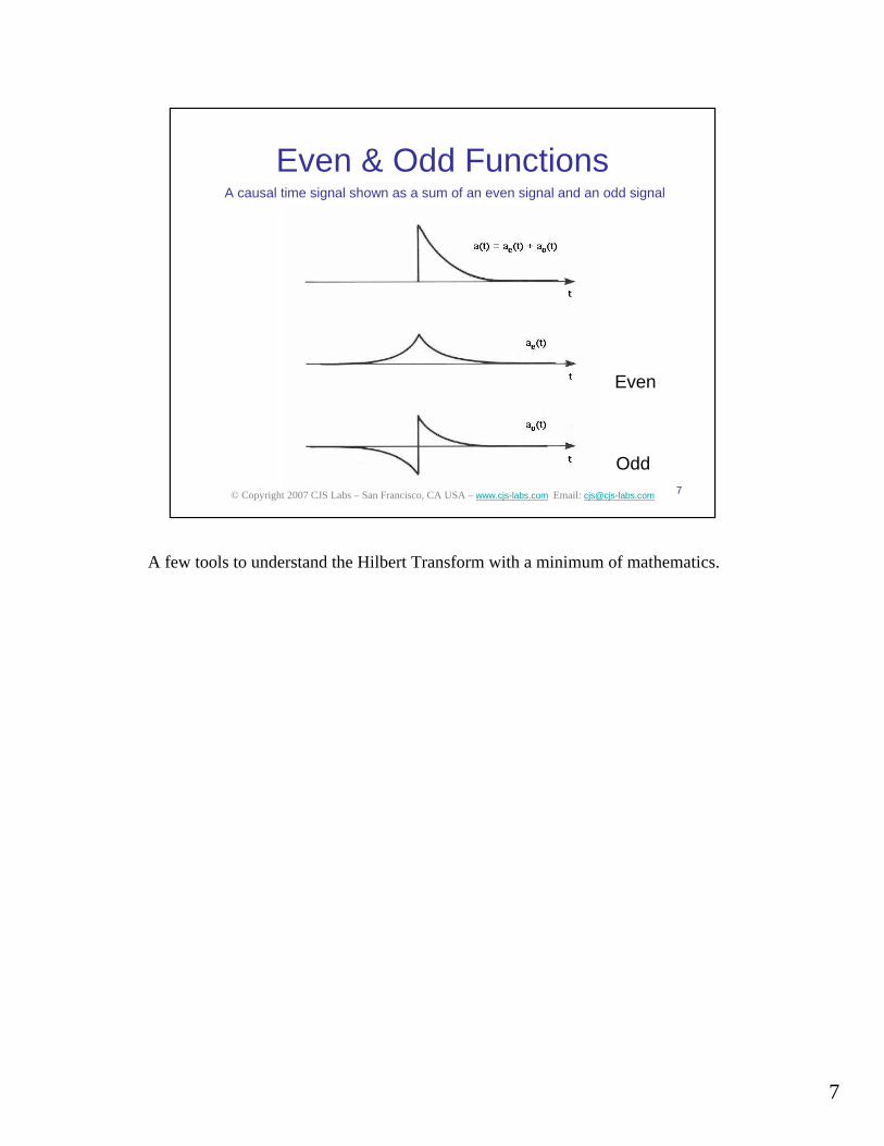
Even & Odd Functions

Even

Odd

A causal time signal shown as a sum of an even signal and an odd signal

A few tools to understand the Hilbert Transform with a minimum of mathematics.

8


Fourier Transform Relationships

R Odd, X EvenImaginary

R Even, X OddReal

Imaginary and OddReal and Odd

Real and EvenReal and Even

a(t) F A(f) = R(f) + jX(f)

From the Symmetry Property of the Fourier Transform: F{F{a(t)}} = a(-t).

9


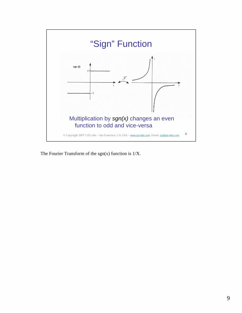
“Sign” Function

Multiplication by sgn(x) changes an even function to odd and vice-versa

The Fourier Transform of the sgn(x) function is 1/X.

10


Frequency Domain

- 90° (-j) for positive frequencies+90° (j) for negative frequencies

)sgn()()](~[ fjfAtaF ⋅−≡

Using these tools, we can write the Hilbert Transform in the Frequency Domain as shown.

11


Effect of Hilbert Transform

Effect of the Hilbert Transform in the Frequency Domain.

12


Hilbert Transform of a Sinusoid

Successive Hilbert Transforms of a sinusoid.

13


Analytic Signal

)t(je)t(a

)t(a~j)t(a)t(a

θ⋅=

+≡∇

∇

Definition of an Analytic Signal and the Envelope Function. The spectrum of the Analytic signal is is one-sided (positive only) and positive valued.

14


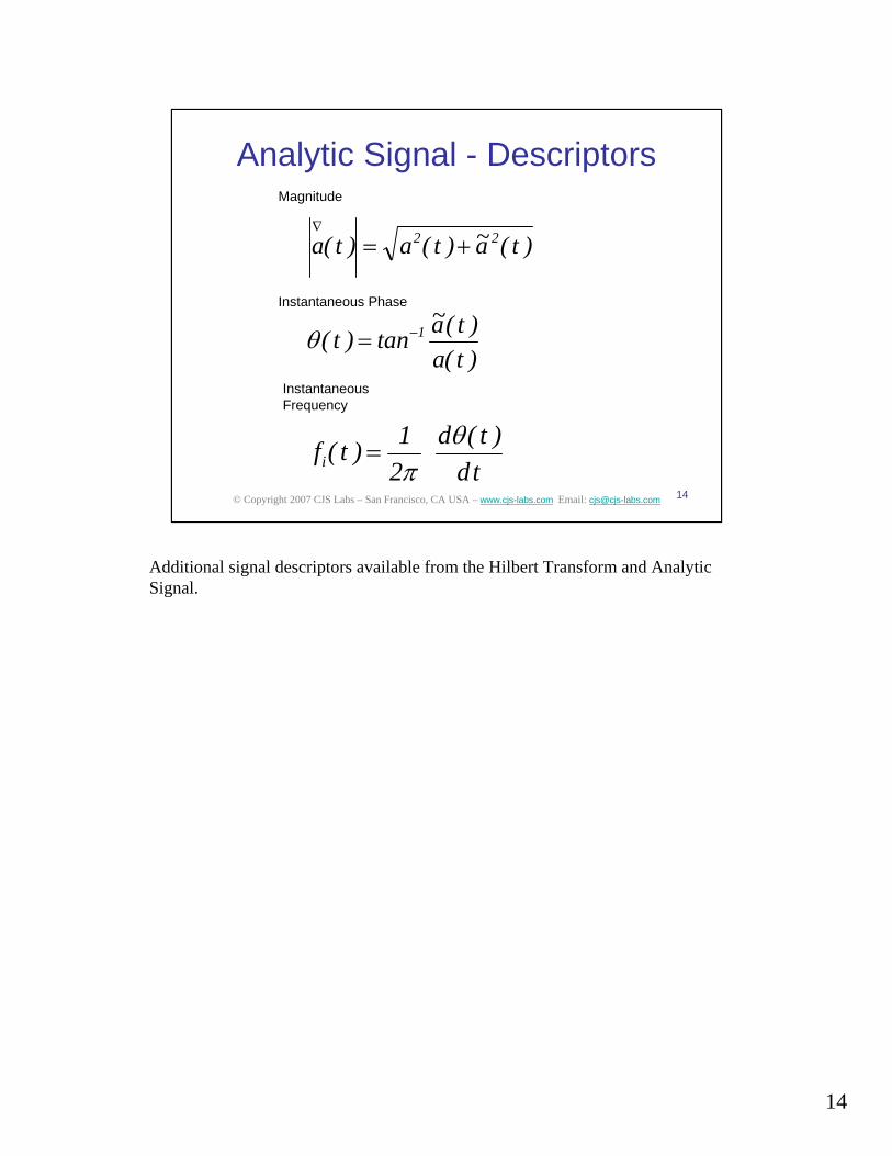
Analytic Signal - Descriptors

)t(a~)t(a)t(a 22 +=∇

)t(a)t(a~tan)t( 1−=θ

Magnitude

td)t(d

21)t(fi

θπ

=

Instantaneous Phase

Instantaneous Frequency

Additional signal descriptors available from the Hilbert Transform and Analytic Signal.

15


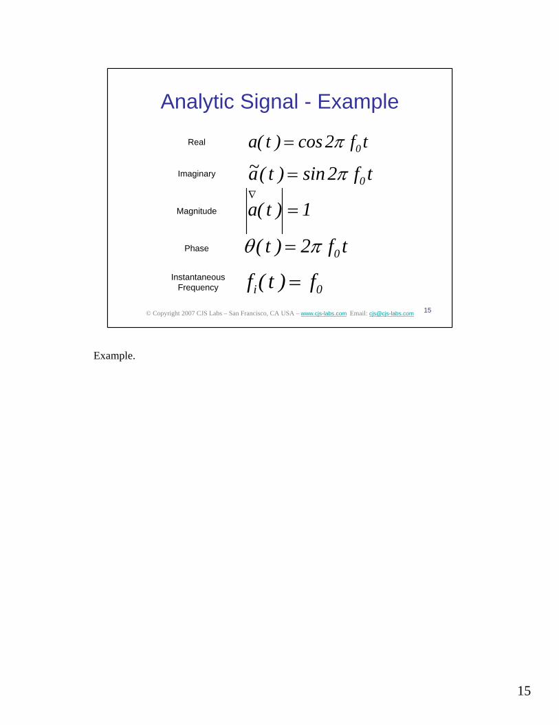
Analytic Signal - Example

0i f)t(f =

tf2)t( 0πθ =

1)t(a =∇

tf2cos)t(a 0π=

tf2sin)t(a~ 0π=

Magnitude

Real

Imaginary

Phase

InstantaneousFrequency

Example.

16


Analytic Signal

Sinusoidal Analytic Signal shown as a “Heyser Spiral”. The Nyquist Plot is the projection along the time axis. The Real and Imaginary parts are the projections along the real and imaginary axes, respectively.

17


Time-Frequency Relationships

Magnitude Real

Phase Imaginary

H F

MagnitudeReal

PhaseImaginary

H †

Time Response h(t) Frequency Response H(f)

InstantaneousFrequency

Group Delaydtd df

d

Time & Frequency relationships of the various descriptors for a causal two-port system response function.

18


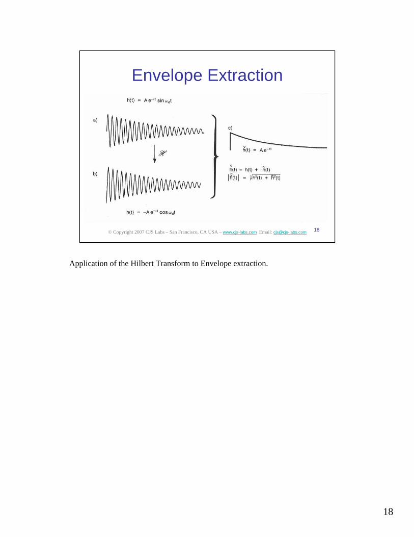
Envelope Extraction

Application of the Hilbert Transform to Envelope extraction.

19


Decay Time Estimation (τ ,T60)Exponentially Decaying SinusoidMagnitude of Analytic SignalLog Magnitude Scale

Application of the Hilbert Transform to Envelope extraction and decay time estimation, RT60 or RC LC circuit time constant, etc. The positive-valued magnitude function can be graphed on a log amplitude scale, enabling a far wider dynamic range than for a real-valued time signal.

20


Propagation Delay / Signal Arrival Estimation

Real Time SignalHilbert Transform of SignalMagnitude of Analytic Signal - Peak indicates arrival time

Application of the Hilbert Transform to Envelope to acoustic signal propagation time estimation.

21


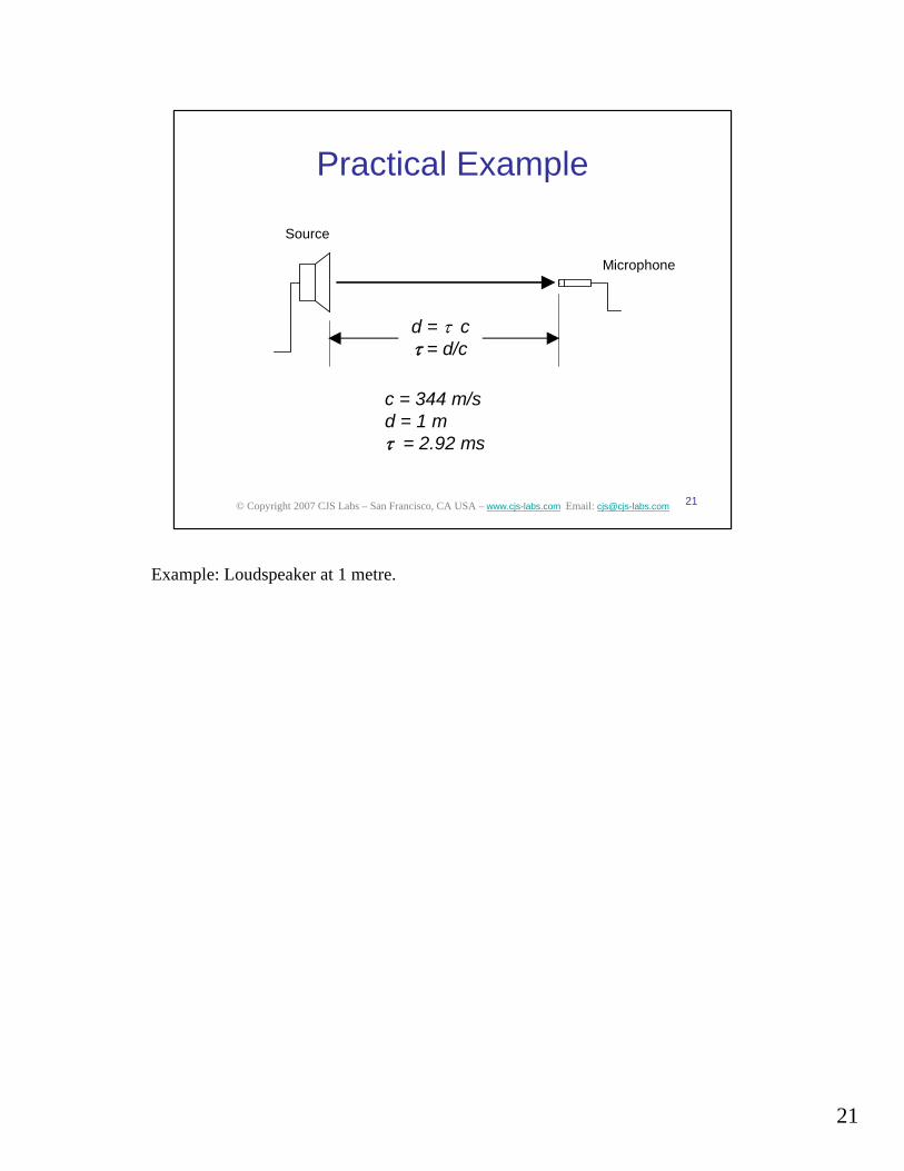
Practical Example

d = τ ·cτ = d/c

Source

Microphone

c = 344 m/sd = 1 mτ = 2.92 ms

Example: Loudspeaker at 1 metre.

22


Loudspeaker Measurement

“Energy-Time Curve” (ETC)

Resulting response without windowing, shown as magnitude in both the Time and Frequency Domains.

23


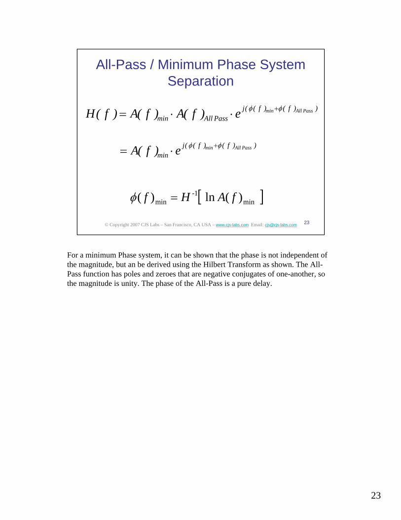
All-Pass / Minimum Phase System Separation

))f()f((jPassAllmin

PassAllmine)f(A)f(A)f(H φφ +⋅⋅=

[ ]min1

min )(ln)( fAHf -=φ

))f()f((jmin

PassAllmine)f(A φφ +⋅=

For a minimum Phase system, it can be shown that the phase is not independent of the magnitude, but an be derived using the Hilbert Transform as shown. The All-Pass function has poles and zeroes that are negative conjugates of one-another, so the magnitude is unity. The phase of the All-Pass is a pure delay.

24


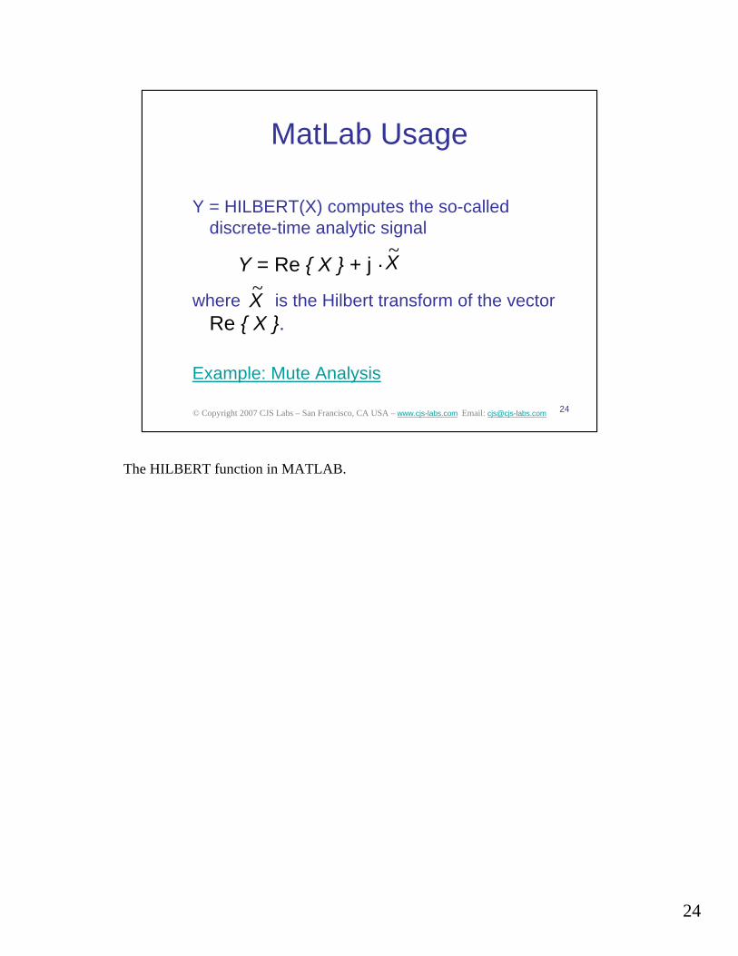
MatLab Usage

Y = HILBERT(X) computes the so-called discrete-time analytic signal

Y = Re { X } + j ·

where is the Hilbert transform of the vector Re { X }.

X~

X~

Example: Mute Analysis

The HILBERT function in MATLAB.

25


Use of the Hilbert Transform:• Allows definition of the analytic signal from a

real-valued time signal:– The Real Part is the original time signal– The Imaginary Part is the Hilbert Transform

• This enables calculation of the envelope(magnitude) of a time signal

• Applications:– Envelope Extraction / Magnitude Estimation– Decay Time Estimation: RT60, τ– Propagation Delay & Signal Arrival Measurements– All-Pass / Minimum Phase System Separation

Conclusion

Conclusion.

the hilbert transform - cjs labs

Documents