application of the european customer satisfaction index … · 1 application of the european...

1

Application of the European Customer Satisfaction Index toPostal Services. Structural Equation Models versus Partial

Least Squares

Christina O’Loughlin*, Germà Coenders †

Departament d’Economia,Universitat de Girona

Girona, September 2002

Abstract

Customer satisfaction and retention are key issues for organizations in today’s competitivemarket place. As such, much research and revenue has been invested in developing accurateways of assessing consumer satisfaction at both the macro (national) and micro(organizational) level, facilitating comparisons in performance both within and betweenindustries. Since the instigation of the national customer satisfaction indices (CSI), partialleast squares (PLS) has been used to estimate the CSI models in preference to structuralequation models (SEM) because they do not rely on strict assumptions about the data.However, this choice was based upon some misconceptions about the use of SEM’s anddoes not take into consideration more recent advances in SEM, including estimationmethods that are robust to non-normality and missing data.

In this paper, both SEM and PLS approaches were compared by evaluating perceptionsof the Isle of Man Post Office Products and Customer service using a CSI format. The newrobust SEM procedures were found to be advantageous over PLS. Product quality wasfound to be the only driver of customer satisfaction, while image and satisfaction were theonly predictors of loyalty, thus arguing for the specificity of postal services.

Keywords: European Customer Satisfaction Index (ECSI), Structural Equation Models,Robust Statistics, Missing Data, Maximum Likelihood.

JEL classification: C13, C39, C51, H42, L89, M11.

* Heart Failure Unit, St. Michael’s Hospital, DunLaoghaire Co. Dublin, Ireland. E-mail: [email protected]† Address: Departament d’Economia. Universitat de Girona, Campus de Montilivi, 17071 Girona, Spain.E-mail: [email protected]

2

1. Introduction

1.1. Origin and Uses of the Customer Satisfaction Index

Customer satisfaction has become a vital concern for companies and organizations intheir efforts to improve product and service quality, and maintain customer loyaltywithin a highly competitive market place. In the last decade, a number of nationalindicators reflecting consumer satisfaction across a wide range of organizations havebeen developed (e.g., Sweden, Fornell, 1992; USA, Fornell et al., 1996; Norway,Andreassen & Lindestad, 1998a, 1998b; Denmark, Martensen, Grønholdt & Kristensen,2000; European Union, ECSI Technical Committee, 1998). At the national level, thecustomer satisfaction index (CSI) is a nationwide gauge of how adequately companies,and industries in general satisfy their customers. In addition, CSI’s can be used at thelower industry or even company level facilitating comparison of companies within anindustry. These indicators complement traditional measures of economic performance(e.g., return on investment, profits and market shares) providing useful diagnosticsabout organizations, and their customers evaluations of the quality of products andservices.

1.2. Factors within the ECSI/ACSI Model

The basic structure of the CSI model has been developed over a number of years and isbased upon well established theories and approaches to consumer behaviour, customersatisfaction and product and service quality (see Fornell, 1992; Fornell et al., 1996). Thestructure of the CSI is continually undergoing review and subject to modifications.Although the core of the model is in most respects standard, there are some variationsbetween the SCSB (Swedish), the ACSI (American), the ECSI (European), the NCSB(Norwegian) and other indices. For example, the image factor is not employed in theACSI model although plans are underway to include this factor into this model (Johnsonet al., 2001).

The CSI model consists of a number of latent factors, each of which isoperationalised by multiple indicators. Customer satisfaction (SATI) can be defined asan overall evaluation of a firm’s post-purchase performance or utilization of a service(Fornell, 1992). It is at the core of the CSI framework and is encased within a system ofcause and effect running from the antecedents of overall customer satisfaction -expectations, image, perceived quality and value – to the consequences of overallcustomer satisfaction – customer loyalty and customer complaints. The obvious strengthof this approach is that it moves beyond the immediate consumption experience andfacilitates the study of the causes and consequences of consumer satisfaction. In fact,the primary objective of this structural approach is to explain customer loyalty.

3

Antecedents of customer satisfaction:1) Perceived Quality: In 1996, the ACSI model was expanded to delineate two general

types of perceived quality, product quality (hardware) and service quality(software/humanware) (Fornell et al., 1996). Perceived product quality (QUAL1) isthe evaluation of recent consumption experience of products. Perceived servicequality (QUAL2) is the evaluation of recent consumption experience of associatedservices like customer service, conditions of product display, range of services andproducts etc. This distinction between service quality and product quality is astandard feature of the ECSI model (Eklöf, 2000). Kristensen et al., (1999)demonstrated the importance of delineating these two aspects of perceived quality ina post office context. Both QUAL1 and QUAL2 are expected to have a direct andpositive effect on overall customer satisfaction.

2) Value (VALU): The literature in this area has recognised that customer satisfaction isdependent on value (Howard & Sheth, 1969). Value is the perceived level ofproduct quality relative to the price paid or the “value for money” aspect of thecustomer experience. Value is defined as the ratio of perceived quality relative toprice (Anderson et al., 1994). Value is expected to have a direct impact onsatisfaction (Anderson & Sullivan, 1993; Fornell, 1992) and to be positivelyaffected by perceived quality (both QUAL1 and QUAL2). To ensure that the effectsof a price-quality relationship are not confounded, quality and value are measuredrelative to each other (Anderson et al., 1994).

3) Image (IMAG): Image refers to the brand name and the kind of associationscustomers get from the product/brand/company. This construct was first introducedin the Norwegian Customer Satisfaction Barometer (NCSB) model (Andreassen &Lindestad, 1998a; Andreassen & Lindestad, 1998b). New research indicates that it isan important component of the customer satisfaction model (e.g., Martensen et al.,2000). It is expected that image will have a positive effect on customer satisfactionand loyalty. In addition, image has been modelled to have a direct effect on value(e.g., Kristensen et al., 1999; Martensen et al., 2000). The impact of quality onimage (or vice versa) is not usually estimated. According to Johnson et al., (2001),image has been modelled to affect perceptions of quality (Andreassen & Lindestad,1998a). However, in most research papers this affect is not modelled, thus weconsider image and product and service quality to be all exogenous factors.

4) Expectations: Expectations refer to the level of quality that customers expect toreceive and are the result of prior consumption experience with a firm’s products orservices. Johnson et al., (2001) noted that the effect of expectations is nonsignificant in a number of industry sectors. Similarly, Martensen et al., (2000)showed that customer expectations of post office products and services in Denmarkhave a negligible impact on consumer satisfaction. Thus, the expectations constructwas not included in this paper.

Consequences of consumer satisfaction:1) Complaints (COMP): This factor refers to the intensity of complaints and the

manner in which the company manages these complaints. It is expected that an

4

increase in customer satisfaction should decrease the incidence of complaints(American Society for Quality, 1998; Fornell et al. 1996).

2) Loyalty (LOYA): Customer loyalty is the ultimate dependent variable in the modeland is seen to be a proxy measure for profitability (Reichheld & Sasser, 1990).Increasing customer loyalty secures future revenues and minimises the possibility ofdefection if quality decreases. In addition, word-of-mouth from satisfied loyalcustomers embellishes the firm’s overall reputation and reduces the cost ofattracting new customers (Anderson & Fornell, 2000). Loyalty is measured byrepurchase intention, price tolerance and intention to recommend products orservices to others. It is expected that better image and higher customer satisfactionshould increase customer loyalty. In addition it is expected that there is a reciprocalrelationship between complaints and loyalty. When the relationship betweencustomer complaints and customer loyalty is positive it implies that the firm issuccessful in turning customers who complain into loyal customers. Conversely, it isexpected that when the relationship is negative the firm has not handled complaintsadequately.

Our model is thus displayed in Figure 1.

IMAG

QUAL1

QUAL2

VALU SATI

LOYA

COMP

Figure 1. CSI model

1.3. Estimation Procedures

From the beginning, Partial Least Squares (PLS, Wold, 1975) has been suggested as amethod for estimating the latent variable CSI models (Fornell, 1992). Thisrecommendation was grounded on the argument that the other widely employedframework used to estimate relationships among latent variables (covariance structure

5

analysis models, also called structural equation models –SEM– and sometimes LISRELmodels, after the name of the first commercial software that became available,developped by Jöreskog, 1973. See Bollen, 1989, Raykov and Marcoulides, 2000; orBatista-Foguet & Coenders, 2000 as introductory manuals) makes more strictassumptions on the data, mainly regarding normality. This recommendation can betraced back to previous PLS literature (e.g. Fornell & Cha, 1994) and seems to havebeen widely followed. The examples of SEM models applied to the CSI are few, theydo not take advantage of the latest developments in SEM (Hackl, Scharitzer & Zuba,2000) and often conclude with a recommendation to use PLS instead (Kristensen,Martensen, & Grønholdt, 1999).

PLS estimates have been reported to be biased (Cassel, Hackl & Westlund, 2000). Infact, from a theoretical point of view, this bias would only disappear under perfectreliability of the observed variables or under an infinite number of indicators per latentvariable. However, the arguments that can be found from the advocates of PLS are various:1) PLS is best suited as a prediction technique. However biased their estimates may be,

they yield optimal predictions of the dependent variables from the observedexplanatory variables. This property is shared with ordinary least squared regression,that is also biased under the presence of measurement error in the explanatoryvariables, but also yields optimal predictions even in this case.

2) SEM assumes that observations are independent and follow a multivariate normaldistribution. PLS uses non-parametric inference methods (such as jackknifing) and isfree of these assumptions.

3) SEM scores for the individuals on the latent variables are indeterminate.

Some of these arguments are fallacious in the CSI context and others have beenrendered outdated as new developments have come into being in the SEM field.1) More often than not, PLS is used in the CSI context with the aims of validating the

measurement instruments in the CSI scales and of estimating and testing the effects onsome dependent variables, purely predictive applications being rare in the literature. Inorder to perform a construct validation, unbiased estimates of factor loadings, factorcorrelations and regression slopes are needed. Factor correlations and regression slopesare reported to have a negative bias (Dijkstra, 1983), thus failing to reveal relationshipsamong factors that are relevant for nomological validation. Factor loadings arereported to be overerestimated and tend to be similar even when true loadings aredissimilar (Widaman, 1993) thus obscuring convergent validation. Even Jacknifeconfidence intervals are of little use when they are built around a biased point estimate.

2) The issue of robustness of SEM estimates was sometimes misunderstood in earlyapplications. Normality and independence of observations are not required forunbiasedness of maximum likelihood (ML) estimates, but are necessary for theirefficiency and for providing correct standard errors and test statistics. However, eventhe later property is unaffected by non-normality if certain conditions are fulfilled(Satorra, 1990). Robust procedures in SEM were considered from an early stage.Browne (1984) suggested an alternative estimation method that is efficient and leads tocorrect test statistics under arbitrary distributions as long as sample sizes are large and

6

the number of variables included in the model is small to moderate (Muthén & Kaplan,1989). Satorra (1990, 1992, 1993) and Satorra and Bentler (1994) developed robuststandard errors and test statistics under arbitrary distributions when using the stillconsistent standard ML estimation method, a solution found to be advantageous forsmaller sample sizes or larger models (Fouladi, 2000). Muthén and Satorra (1995)extended the former robust statistics to complex samples, the commonest source ofdependence among observations in survey data. Finally, statistical inference based onnon parametric resampling methods (e.g. bootstrap) is equally possible for SEM as it isfor PLS (see Nevitt & Hancock, 2001 for an evaluation of its performance).

3) PLS latent variable scores are computed in such a way that the reliability estimates ofthe indicators and the R2 of the latent variable regressions are maximised (Fornell &Cha, 1994). This criterion is indeed objective but it can be considered to be responsiblefor the bias in PLS parameter estimates, as some of the parameters (error variances) areminimized as a part of the criterion function. In SEM, the parameters are firstconsistently estimated and next latent variable scores are estimated conditional onthese parameters. The fact that several criteria or objective functions are available fordoing this, and that they differ from the equally arbitrary PLS criterion, does notprovide adequate reason to refer to these scores as indeterminate. The most commonapproach is regression, which is equivalent to maximising the reliability of the latentvariable scores and is very appealing from a practical point of view whenever the aimof the research is the development of indices. As an alternative, latent variable scorescan be computed so that their means, covariances and variances are as close as possibleto the model estimated means, variances and covariances of the latent variables. Othermethods are also available (see Bollen, 1989, p 305, and references therein).

Besides, SEM have also a number of advantages over PLS that must not be ignored:1) SEM offer the possibility of testing the significance of omitted parameters (e.g. Bollen

& Long, 1993), such as error covariances and loadings on more than one latentvariable. Such parameters compromise validity if significant, as they show indicatorsto contain some common variance unrelated to the latent variable they are supposed tomeasure (Batista-Foguet & Coenders, 1998).

2) SEM offer more flexibility in the specification of the model parameters, like forinstance the error covariances and loadings on more than one latent variable mentionedabove (e.g. Coenders & Saris, 2000).

3) SEM make it possible to simultaneously estimate the same model in severalpopulations.

4) SEM make it possible to use the statistical theory that is coupled with maximumlikelihood estimation.

5) SEM allow researchers to constrain parameters to be equal to a given value or to agiven linear or non-linear function of other parameters.

7

Finally, additional developments in SEM have rendered this approach far moregeneral and flexible than PLS. These include:1) Inclusion of observed variables with an ordinal measurement level (Muthén, 1984;

Jöreskog, 1990; Coenders & Saris, 1995; Coenders, Satorra & Saris, 1997). PLSassumes interval measured observed variables.

2) Treatment of hierarchical two-level data structures, thus bringing together SEM andsome forms of multilevel modelling (Muthén, 1994).

3) Inclusion of both latent and observed categorical variables, thus bringing togetherSEM, mixture models and latent class models (Muthén, 2001). PLS assumesinterval measured observed and latent variables.

4) ML estimation with missing data (Allison, 1987; Muthén, Kaplan, & Hollis, 1987;Wothke, 2000; Muthén & Muthén, 2001; Graham, Taylor & Cumsille, 2001).Variants of the method that are robust to non normality have recently becomeavailable (Yuan & Bentler, 2000). PLS requires a complete data set, which makesonly imputation, mean substitution and listwise deletion appropriate.

All these developments have reached the stage of wide acceptance and availabilityand are all currently available to the user in at least one of the last generationcommercial SEM software programs, that are all very user friendly and no longerrequire matrix algebra knowledge from the user.

1.4. Plan of the Paper

This paper illustrates the use of both PLS and recent SEM estimation procedures thatare robust to non-normality and consistent under incomplete data missing at random.The illustration utilises data from an administration of the ECSI questionnaire in anindustry specific case, the postal services of the Isle of Man.

The paper will be organised as follows. First the data and questionnaire will bepresented. Then seven alternative SEM estimation procedures will be discussed. Next aconfirmatory factor analysis will be used to validate the questionnaire and will beestimated using the seven procedures and the results compared. The causal relationshipsbetween dimensions in the ECSI model will then be estimated using the best of themethods. After removal of non significant effects the results will be interpreted and theimplications, both statistical and theoretical, discussed.

2. Method

2.1. The Measurement Instrument

A number of CSI questionnaire formats, including the ECSI and ACSI were examinedto aid in the development of a survey instrument relevant to the Isle of Man Post Office.

8

In addition, Post Denmark supplied a copy of their questionnaire, the results of whichwere documented by Kristensen, Martensen and Grønholdt (1999). Excellence Irelandsupplied copies of questionnaires used to assess CSI in the mobile phone and bankingsectors in Ireland.

Latent variable Observed variablesQUALITY OF PRODUCTS:HARDWARE (QUAL1)

Q1. Please rate the overall quality of products and servicesQ2. Please rate the quality of products and services compared to thequality offered by similar companiesQ3. Does the overall quality of products meet your quality requirements?Q8. Could the quality of the products and services be improved?Q12. In the last 6 months how often have things actually gone wrongwith the products/services you use?

QUALITY OF CUSTOMERSERVICE: HUMANWARE(QUAL2)

Q4. Please rate the overall quality of customer serviceQ5. Please rate the quality of customer service compared to the qualityoffered by similar companiesQ6. Does the overall quality of customer service meet your qualityrequirements?

PERCEIVED VALUE (VALU) Q7. Please rate the quality of products/services given the prices you payQ10. Please rate the prices of products and services given the quality

IMAGE (IMAG) Q20. The PO is a financially sound companyQ21. The PO is a reliable and trustworthy companyQ22. The PO is a customer-oriented companyQ23. The PO provides a valuable service to the communityQ24. The PO is innovative and forward lookingQ25. The PO uses modern technological equipment and proceduresQ26. The PO premises are modern and visually appealingQ27. The PO is a competitive courier service providerQ28. The PO offers value for money

CUSTOMER SATISFACTION(SATI)

Q15. Overall how satisfied are you with the PO products and services?Q16. How close is the PO to your ideal postal service provider?Q17. Considering your expectations, to what extent has the PO fallenshort of or exceeded your expectations?

CUSTOMER LOYALTY(LOYA)

Q11. If there was a competitive postal service provider that could offerthe same range and quality of products/services as the PO how muchwould they have to reduce their prices for you to change provider?Q18. If you required new postal/courier products or services how likelyis it that you would choose the PO to provide you with these services?Q19. If asked for your advice, how likely is it that you would recommendthe PO services you use to others?

CUSTOMERCOMPLAINTS

Q13. How many times have you complained (either formally orinformally) to PO personnel?Q14. How well or poorly was your most recent complaint handled?

Table 1: Isle of Man Post Office postal survey containing items pertaining to this articleonly. Questions in italics are absent from the final model

The first draft of the survey was issued to 30 individuals to examine the questionwording and relevance. Feedback from this pilot study indicated that some questionswere ambiguous, difficult to understand, or irrelevant in a Postal context and werereworded. The final questionnaire contained 28 questions pertaining to the global

9

customer satisfaction index, 38 specific questions about products and services, and 3demographic questions. Only questions relating to the global customer satisfactionindex are discussed in this paper and are displayed in Table 1. Questions are rated on 1to 10-point scale with the exception of Q11 and Q13.

2.2. Sample and Data Collection

The questionnaire was administered to an Isle of Man residential sample. Data werecollected during the summer of 2001 using a postal data collection mode (for anoverview of competing data collection modes and their cost/quality balance see forinstance Groves, 1989). It was unnecessary to use screening questions as all residents onthe Island are in receipt of a postal service. One thousand residential clients wererandomly selected from The Isle of Man Electoral Register where all constituency areaswere proportionally represented. As specified in ECSI/ACSI methodologies, responseswere made on a 10 point scale. A total of 28% of this sample completed and returnedthe questionnaires, which is quite a good result for the postal administration method. Onaverage, all constituencies were proportionally represented by this sample. Within eachconstituency, simple random sampling was used, which ensures approximateindependence of observations.

2.3 Exploratory Analyses and Estimation Procedures

Univariate and bivariate sample statistics were first computed. The complaint dimension(Q13, Q14) was dropped from the model as 86% of respondents had not complainedduring the previous 6 months. Q12 was removed because of low correlations with otheritems in the QUAL1 dimension.

In order to prevent the effects of outliers on the results of multivariate statisticalmodels (Barnett & Lewis, 1994), we computed the Mahalanobis distance to the meanvector (Mahalanobis, 1936) and removed 4 observations with extreme values.

As regards normality, many variables showed evidence of moderate to severenon-normality, as shown in Table 2.

Prior to performing estimation, variables (Q2, Q5, Q11, Q20, Q25, Q27) andcases with more than 25% missing data were deleted. Variables with larger proportionof missing data can be assumed to be meaningless to a portion of the population. Caseswith a larger proportion of missing data can be assumed to correspond either to carelessrespondents or to infrequent users of the service. The effective sample size was 258.The distribution of the remaining missing data was as shown in Table 3, and amount to anoverall rate of missingness of 4.2%.

10

Variable Mean St. Dev. Skewness KurtosisQ1 8.292 1.642 -0.965** 1.093**Q3 8.396 1.700 -1.046** 0.691Q4 8.488 1.682 -1.145** 1.143**Q6 8.432 1.697 -1.124** 1.101**Q7 7.663 1.832 -0.632** 0.096Q8 7.184 2.576 -0.739** -0.356Q10 7.643 1.869 -0.508** -0.305Q15 8.436 1.671 -1.170** 1.122**Q16 8.190 1.764 -0.871** 0.169Q17 7.431 1.872 -0.618** 0.314Q18 8.096 2.094 -1.618** 2.846**Q19 8.213 1.895 -1.345** 1.877**Q21 8.488 1.777 -1.478** 2.260**Q22 7.833 2.109 -0.988** 0.673Q23 9.044 1.398 -2.267** 7.212**Q24 7.550 2.157 -0.768** 0.070Q26 6.473 2.407 -0.333* -0.585**Q28 7.907 1.979 -1.156** 1.472**Table 2: Univariate summary statistics and normality tests

** Skewness or kurtosis significant at the 1% level* Skewness or kurtosis significant at the 5% level

Q1 Q3 Q4 Q6 Q7 Q8 Q10 Q15 Q163 4 2 3 10 29 15 1 11

Q17 Q18 Q19 Q21 Q22 Q23 Q24 Q26 Q2827 18 14 3 8 2 28 10 6

Table 3: Number of missing values per variable

Missing data are treated in several alternative ways within the context of SEM.1) Listwise or pairwise deletion. These procedures are only unbiased if the data are

missing completely at random (see Little and Rubin, 1987). Data are said to bemissing completely at random when the probability that a datum is missing isindependent of any characteristic of the individual. Even under this unrealisticassumption, the first of the mentioned methods is highly inefficient and the secondleads to biased standard errors (Enders, 2001; Enders & Bandalos, 2001). Thismethod is feasible, though of course not recommended, both for SEM and for PLS.

2) Mean substitution. This method is known to bias variances and covariances evenwhen data are missing completely at random (Graham, Hofer & Piccinin, 1994;Graham, Hofer & MacKinnon, 1996, Enders, 2001) and thus should not be used,though numerically speaking is feasible both for SEM and for PLS.

3) Imputation. This is a family of methods including regression imputation, hot deckimputation or EM imputation, in both their simple and multiple variants (Little andRubin, 1987). This approach has the advantage of providing a complete data set onwhich standard estimation procedures could in principle be used. However, some ofthese imputation procedures (simple hot deck imputation and simple regressionimputation) lead to biased estimates of factor correlations and residual variances.

11

Multiple imputation (Rubin, 1987) does not have these drawbacks but it iscumbersome to perform unless special software is available. Imputation can bejustified both if the data are missing at random or completely at random. Data aresaid to be missing at random when the probability that a datum is missing dependsonly of characteristics of the individual that are observed (not missing). This methodis feasible both for SEM and for PLS.

4) Direct ML assuming that the data are normally distributed and missing at random.This procedure is currently available in most of the latest commercial softwarepackages for SEM like Mx (Neale et al., 1999), EQS 6.0 (Bentler, 2000), AMOS 4.0(Aburckle & Wothke, 1999), LISREL 8.51 (Jöreskog et al. 2000; du Toit & du Toit,2001) and MPLUS 2.1 (Muthén & Muthén, 2001). This procedure uses all availabledata to build a case per case likelihood function. It is consistent, efficient and leads tocorrect standard errors and test statistics if the data are normal and missing atrandom (Aburckle, 1996; Enders, 2001; Enders & Bandalos, 2001; Wothke, 2000).Yuan and Bentler (2000) describe other related approaches: a two-stage estimatorbased on the combination of the EM algorithm and a standard ML SEM estimator,and a minimum χ2 estimator. Both approaches seem to have similar properties to thedirect ML estimator. Except for the two-stage EM approach, these methods are onlyfeasible for SEM.

5) A variant of the direct ML estimator with missing data described by Yuan andBentler (2000) is robust to non-normality but assumes data to be missing completelyat random and can be biased otherwise. This method is available at least in MPLUS2.1 and EQS 6.0. The few studies conducted to date report that this method performsquite well, regarding both unbiasedness and standard errors, even when data are justmissing at random (Enders, 2001). This method is only feasible for SEM.

When data are missing not at random (what is also called non-ignorable missingdata) none of the procedures are consistent. This is the case when the probability that adatum is missing depends on characteristics of the individual that are missing, forinstance on the same variable that is missing for the individual. However, ML isreported to be less biased than the alternative approaches (Muthén et al., 1987).

In this article we use SEM under six different approaches and, for comparativepurposes, PLS is also applied using one of these approaches:1) Direct robust ML assuming that the data are missing at random. This is the method

that is correct under the weakest assumptions and is considered as a baseline for thecomparison.

2) Direct standard ML assuming that the data are normally distributed and missing atrandom.

3) Robust ML on a complete data set obtained by a form of imputation that is related tosimple hot deck imputation. For each case (recipient) with a missing datum,complete cases on a given set of related variables are selected. The case with thelowest distance to the recipient on the set of related variables is chosen as a donorfor the missing datum. If more than one potential donor has the same minimumdistance to the recipient, then the mean value for all donors is imputed but this is

12

only done if the variance of these values is lower than the variance of the imputedvariable. This method is currently available in the PRELIS program from version 2on (Jöreskog & Sörbom, 1993). The variables in the model with less than 5 missingcases were used as the set of related variables, together with external variablesrelated to the frequency of use of a set of postal services, for which there were nomissing data. 8 cases could not be imputed because no cases with complete data forthe set of related variables were available or because the variance of the values ofthe donors was larger than the variance of the recipient variable. The final usablesample size was 250.

4) Standard ML on the above imputed data set.5) Robust ML on a complete data set obtained by mean substitution.6) Standard ML estimation on the mean substituted data set. This method is by far the

worst of the six described so far and would be close to what was available for SEMin the early 1980's, that is when PLS were developed and recommended.

7) PLS on the mean substituted data set, with 100 jackknife resamples, using the pathweighting scheme for the inner part of the model, selecting an outward measurementmodel for the outer part of the model and using the non-standardized data. PLScould have been used on the imputed data set as well, but the only aim of includingit here is to compare the results of SEM and PLS on the same data set, for whichpurpose the mean substituted data are enough. Besides, the standard guidelines forthe estimation of the ESCI model include the use of mean substitution.

The PLS estimations were carried out using the PLS-PC 1.8 program. All SEMestimations were carried out with the M-PLUS 2.1 program (Muthén & Muthén, 2001).Point estimates are the same for robust and non-robust SEM estimation methods. This isdue to the fact that standard ML estimates are consistent under non-normality (if a propermissing value treatment is employed, of course) and will be used to save space whenpresenting the results. As regards robust test statistics for complete imputed data M-PLUS computes Satorra and Bentler’s (1994) mean-and-variance adjusted χ2 statistic andalso performs an adjustment of the associated degrees of freedom. When the same is donefor incomplete data, MPLUS computes Yuan and Bentlers T2

* χ2 mean scaled statistic(Yuan and Bentler, 2000), which does not involve any adjustment of the degrees offreedom. Both robust test statistics are robust to non-normality. Standard errors robust tonon-normality are also provided. In the missing data case these robust standard errors arebased on a sandwich procedure (Arminger & Sobel, 1990). Likelihood ratio χ2 differencetests between nested models cannot be carried out with mean-and-variance adjusted χ2

statistics but they can be obtained for mean scaled χ2 statistics if some simple calculationsare performed by hand (Satorra & Bentler, 1999). Let T2

*0 and T2

*1 be the mean scaled χ2

statistics, c0 and c1 the scaling constants, and d0 and d1 the degrees of freedom for twonested models, of which Model 0 is more restrictive. This implies that the standard ML χ2

statistics are T0= T2*0c0 and T1= T2

*1c1. The robust χ2 difference can be computed as:

13

)( 10

1100

102

ddcdcd

TTdifferenceRobust

−−−

=χ

3. Results

3.1. Confirmatory Factor Analysis Model

As often recommended (e.g. Bollen, 1989, Batista-Foguet & Coenders, 2000), aconfirmatory factor analysis (CFA) model was first fit to assess the quality of theindicators of the underlying factors and spot invalid items that do not only measure theintended factor but have other systematic sources. During this process, Q26 wasdropped as it was the indicator of the image factor with the largest error variance as wellas being involved in the three highest residual covariances, which suggests that the itemmeasures other things than only image. Q28 was also dropped as it loaded on both thevalue and image factors, which was not unexpected given its wording. These problemscan be detected in a straightforward manner in SEM, as the significance of omittedparameters is being tested. Had PLS been used, they would have gone unnoticed. Thefinal CFA model is displayed in Figure 2.

Q1 Q3 Q8

QUAL1

Q4 Q6

QUAL2

Q7 Q10

VALU

Q18 Q19

LOYA

Q15 Q16 Q17

SATI

Q21 Q22 Q23

IMAG

Q24

Figure 2: CFA model

14

Hot deck imputationQ1 Q3 Q4 Q6 Q7 Q8 Q10 Q15 Q16 Q17 Q18 Q19 Q21 Q22 Q23 Q24

Q1 2.70Q3 2.11 2.89Q4 1.80 1.93 2.83Q6 1.98 2.18 2.48 2.88Q7 1.87 2.18 1.82 2.09 3.36Q8 2.54 2.86 2.34 2.71 2.93 6.63Q10 1.83 2.16 1.79 2.06 2.67 2.97 3.49Q15 1.96 2.34 1.96 2.13 2.20 2.96 2.13 2.79Q16 1.79 1.95 1.67 1.80 1.81 2.68 1.95 2.17 3.11Q17 1.76 2.05 1.68 1.94 2.09 2.87 2.23 2.24 1.94 3.50Q18 1.64 1.94 1.57 1.84 1.87 2.37 1.67 1.96 1.97 1.95 4.38Q19 1.90 2.18 1.87 2.09 2.06 2.63 2.16 2.19 2.02 2.13 2.71 3.59Q21 1.72 1.98 1.74 1.86 1.89 2.51 2.00 1.93 1.82 1.92 1.79 2.17 3.16Q22 2.13 2.33 2.25 2.38 2.31 3.20 2.36 2.41 2.24 2.50 2.57 2.81 2.84 4.45Q23 1.18 1.32 1.33 1.42 1.37 1.49 1.37 1.27 1.18 1.24 1.46 1.61 1.44 1.72 1.95Q24 1.98 2.35 2.12 2.28 2.44 3.25 2.46 2.42 2.35 2.59 2.23 2.38 2.42 3.63 1.52 4.65

ML with missing dataQ1 Q3 Q4 Q6 Q7 Q8 Q10 Q15 Q16 Q17 Q18 Q19 Q21 Q22 Q23 Q24


Mean imputationQ1 Q3 Q4 Q6 Q7 Q8 Q10 Q15 Q16 Q17 Q18 Q19 Q21 Q22 Q23 Q24


Table 4: Covariance matrices obtained under 4 alternative missing data treatments

15

The results of the final CFA model are compared for the seven estimationmethods. Table 4 shows the estimated sample covariances. It can easily be seen thatcovariances obtained under imputation or ML are very similar. This argues for thequality of the imputation, though it can also be a result of the low rate of datamissingness. On the contrary, variances and covariances resulting from meanimputation are in some cases considerably lower, especially when covariances involvepairs of variables with a sizeable amount of missing data. In SEM, biased covariancescan only lead to biased parameter estimates.

Table 5 shows the estimates and goodness of fit statistics of the CFA modelshown in the path diagram of Figure 2 using the seven methods. Several goodness of fitmeasures are usually considered in SEM (Bollen & Long, 1993). A likelihood ratio χ2

test of the hypothesis that all model constraints hold in the population is usuallyperformed first. Here we notice the first differences across methods. All procedures thatare not robust to non-normality clearly lead to the rejection of the model's constraints.For ML with robust test statistics, the hypothesis is also rejected but by a narrowermargin. Usually researchers are not so interested in exactly fitting models, so thatquantitative measures of misfit are preferred to tests of exact fit. A wealth of fitmeasures have been suggested. Among the most widely used ones are the Root MeanSquared Error of Approximation (RMSEA), the Tucker and Lewis Index (TLI), alsoknown as Non Normed Fit Index, and the root mean squared residual correlation(RMSR). RMSEA and TLI take the parsimony of the model into account, so that thereleasing of approximately correct constraints does not necessarily improve the valuesof these indices. Values of RMSEA and RMSR below 0.05 and values of TLI above0.95 are usually considered acceptable, though the debate concerning which goodnessof fit measures to use and what the threshold for a good model can be is far fromresolved (see Bollen & Long, 1993 for details). Using these measures, the model looksacceptable, but even more so when robust methods are considered. None of these fitindices are available for PLS. PLS focuses only on predictive fit measures that, exceptfor the error variances and the standardized loadings, are irrelevant with the purpose ofvalidating a questionnaire using a CFA model. The next part of the table shows thepoint estimates (raw and standardized; they are identical for robust and non-robustmethods using the same missing value treatment) and the standard errors (robust andstandard ML). Three types of parameters are present: factor loadings, factor correlationsand error variances. Standardized error variances are equal to one minus the R-square ofeach measurement equation. Within each parameter type, averages of the relevantstatistics are also shown.

The point estimates obtained from imputed data or by direct ML with missingdata are generally very similar. This could be expected from the fact that covariancesare also similar. The only exception to this is the factor correlations. Simple imputationmethods such as hot deck are known to inflate correlations. However, on average thedifferences are not dramatic. Overall, it looks as if there is not much to be gained byusing direct ML with missing data when the proportion of data that are missing is low.Conversely, there seems to be a great deal to be lost out of using obsolete missing datatreatments such as mean imputation. Nearly all unstandardized factor loadings are lower

16

than for any other of the three methods, and nearly all unstandardized error variancesare higher. The differences are larger for variables with a larger proportion of missingcases.

Non robust ML standard errors are known to underestimate true standard errorswhen most variables have a positive kurtosis. This seems to be the case for our data setand for all missing value treatments, as robust standard errors are higher in nearly allcases, for some parameters more than twice as high. The failure to use robust standarderrors may thus result in confidence intervals that do not contain the true parametervalue or in inflated t-values rejecting true null hypotheses. The advocates of PLS couldnot be more right in claiming that non-normality was a key issue in SEM.

As regards robust standard errors, they are relatively similar across missingvalue treatments. It is known that imputation leads to an underestimation of uncertainty,regardless of whether it is done with mean substitution or hot deck methods (onlymultiple imputation is immune to this). This is also observed here, although differencesare not very large (nearly zero for factor loadings and in the neighbourhood of 10% forthe remaining parameter types). The sample size drops from 258 to 250 for the hot deckcase, but the effect of such a small sample size change on the above results wouldhardly go noticed, as the root of the sample size ratio is only 1.015; thus accounting foronly 1.5% difference in standard errors.

For our data set, that contains a small amount of missing data but severely non-normal data, the use of an imputation method and an estimation method with robuststandard errors and test statistics seems to be a wise second-best option for thoseresearchers who do not have the latest software available.

As regards PLS, its results can be compared to the SEM results using the samedata, that is, the mean imputed data, and tests robust to non-normality. We find thatloadings are systematically higher for PLS and the factor correlations and the errorvariances systematically lower. Besides, loadings on the same factor are more similarunder PLS than under SEM. The differences between SEM and PLS are higher thanbetween any pair of SEM methods, and can be attributed to the well known fact thatPLS is only consistent for an infinite number of indicators per latent variable, as non-normality does not affect the consistency of SEM estimates (Satorra 1990, 1992, 1993,Browne, 1984; Fouladi, 2000; Nevitt & Hancock, 2001). When validating aquestionnaire using a CFA model, PLS can result in retaining items with an apparentlyhigh but actual low loading and can also result in related factors appearing unrelated.This result can be understood because for CFA models, PLS yields exactly the sameestimates as principal component analyses done separately for each dimension. Standarderrors cannot be compared to SEM standard errors, as different estimation procedurescan also differ in precision. They can anyway be trusted as the jackknife procedure isrobust to non normality. However, one may wonder about the use of getting the correctstandard errors for the wrong point estimates. PLS were also used on imputed data andcompared to SEM on imputed data with robust standard errors with identicalconclusions. The results are available from the authors on request.

17

ML with missing data ML on imputed data ML on mean substituted data PLS on mean subst.Test statistics robust ML robust ML robust MLχ2 125.51 153.04 58.80 157.83 62.78 166.15d.f. 89 89 42 89 43 89p-value 0.007 0.000 0.044 0.000 0.026 0.000RMSEA 0.040 0.053 0.040 0.056 0.042 0.058SRMR 0.029 0.029 0.029 0.029 0.029 0.029TLI 0.978 0.975 0.982 0.973 0.978 0.969

estim stand.estim.

robusts. e.

MLs. e.

estim stand.estim.

robusts. e.

MLs. e.

estim stand.estim.

robusts. e.

MLs. e.

estim stand.estim.

robusts. e.

LoadingsQ1 on QUAL1 1.34 0.82 0.091 0.085 1.34 0.82 0.090 0.086 1.31 0.81 0.089 0.085 1.26 0.78 0.100Q3 on QUAL1 1.53 0.90 0.091 0.084 1.53 0.90 0.092 0.085 1.50 0.89 0.089 0.084 1.40 0.83 0.120Q8 on QUAL1 1.98 0.76 0.130 0.147 1.93 0.75 0.129 0.140 1.73 0.70 0.133 0.136 2.29 0.91 0.130Q4 on QUAL2 1.48 0.89 0.103 0.083 1.49 0.89 0.105 0.085 1.48 0.89 0.102 0.082 1.61 0.97 0.080Q6 on QUAL2 1.66 0.98 0.096 0.079 1.66 0.98 0.096 0.080 1.65 0.98 0.095 0.079 1.64 0.97 0.080Q7 on VALU 1.70 0.90 0.100 0.096 1.63 0.89 0.101 0.094 1.65 0.89 0.100 0.094 1.75 0.94 0.090Q10 on VALU 1.69 0.90 0.089 0.096 1.63 0.87 0.090 0.097 1.61 0.88 0.091 0.094 1.74 0.94 0.070Q15 on SATI 1.55 0.93 0.096 0.080 1.55 0.93 0.099 0.081 1.54 0.93 0.096 0.080 1.50 0.90 0.090Q16 on SATI 1.40 0.77 0.101 0.099 1.38 0.78 0.100 0.095 1.36 0.76 0.100 0.096 1.56 0.87 0.100Q17 on SATI 1.44 0.77 0.118 0.105 1.44 0.77 0.115 0.101 1.35 0.75 0.117 0.097 1.55 0.86 0.100Q18 on LOYA 1.63 0.77 0.149 0.119 1.56 0.74 0.145 0.118 1.54 0.75 0.145 0.114 1.92 0.94 0.130Q19 on LOYA 1.81 0.95 0.129 0.098 1.73 0.92 0.135 0.100 1.69 0.92 0.131 0.096 1.65 0.90 0.160Q21 on IMAG 1.44 0.82 0.130 0.093 1.45 0.82 0.131 0.094 1.42 0.81 0.130 0.092 1.47 0.84 0.130Q22 on IMAG 1.92 0.91 0.114 0.104 1.93 0.92 0.116 0.104 1.86 0.90 0.119 0.103 1.95 0.94 0.090Q23 on IMAG 0.96 0.68 0.122 0.079 0.94 0.68 0.127 0.080 0.97 0.69 0.126 0.078 0.97 0.69 0.150Q24 on IMAG 1.79 0.82 0.119 0.117 1.79 0.83 0.112 0.113 1.61 0.78 0.124 0.110 1.81 0.88 0.100

Average 1.58 0.85 0.111 0.098 1.56 0.84 0.111 0.097 1.52 0.83 0.112 0.095 1.63 0.88 0.108Factor correlationsQUAL1withQUAL2 0.87 0.87 0.036 0.023 0.86 0.86 0.035 0.024 0.87 0.87 0.035 0.023 0.72 0.72 0.045QUAL1 with VALU 0.86 0.86 0.029 0.027 0.88 0.88 0.027 0.026 0.86 0.86 0.028 0.028 0.73 0.73 0.039QUAL1 with SATI 0.95 0.95 0.020 0.017 0.96 0.96 0.016 0.016 0.96 0.96 0.019 0.017 0.79 0.79 0.036QUAL1 with LOYA 0.77 0.77 0.060 0.036 0.81 0.81 0.051 0.034 0.79 0.79 0.055 0.037 0.62 0.62 0.047QUAL1 with IMAG 0.84 0.84 0.034 0.027 0.84 0.84 0.031 0.027 0.85 0.85 0.030 0.027 0.72 0.72 0.043QUAL2 with VALU 0.74 0.74 0.042 0.034 0.76 0.76 0.041 0.033 0.73 0.73 0.042 0.035 0.66 0.66 0.036QUAL2 with SATI 0.81 0.81 0.045 0.028 0.82 0.82 0.040 0.027 0.80 0.80 0.041 0.028 0.70 0.70 0.041QUAL2 with LOYA 0.68 0.68 0.068 0.041 0.72 0.72 0.063 0.039 0.68 0.68 0.065 0.041 0.59 0.59 0.056QUAL2 with IMAG 0.77 0.77 0.045 0.031 0.77 0.77 0.043 0.031 0.77 0.77 0.042 0.031 0.71 0.71 0.042VALU with SATI 0.84 0.84 0.030 0.028 0.86 0.86 0.029 0.026 0.85 0.85 0.029 0.027 0.74 0.74 0.037VALU with LOYA 0.70 0.70 0.065 0.042 0.74 0.74 0.056 0.041 0.70 0.70 0.059 0.043 0.57 0.57 0.053VALU with IMAG 0.77 0.77 0.039 0.034 0.79 0.79 0.037 0.033 0.78 0.78 0.038 0.034 0.69 0.69 0.038SATI with LOYA 0.81 0.81 0.064 0.033 0.83 0.83 0.055 0.032 0.82 0.82 0.057 0.033 0.69 0.69 0.035SATI with IMAG 0.84 0.84 0.037 0.026 0.85 0.85 0.033 0.025 0.85 0.85 0.034 0.026 0.77 0.77 0.033LOYA with IMAG 0.82 0.82 0.050 0.031 0.84 0.84 0.049 0.031 0.83 0.83 0.050 0.032 0.69 0.69 0.054

Average 0.80 0.80 0.044 0.031 0.82 0.82 0.040 0.030 0.81 0.81 0.042 0.031 0.69 0.69 0.042Error VariancesQ1 0.88 0.33 0.313 0.090 0.90 0.33 0.289 0.092 0.92 0.35 0.276 0.093 1.03 0.39Q3 0.55 0.19 0.082 0.072 0.55 0.19 0.078 0.071 0.61 0.21 0.088 0.076 0.91 0.32Q4 0.59 0.21 0.091 0.074 0.60 0.21 0.089 0.075 0.58 0.21 0.090 0.073 1.02 0.16Q6 0.13 0.04 0.074 0.066 0.12 0.04 0.072 0.066 0.14 0.05 0.072 0.066 0.19 0.07Q7 0.67 0.19 0.126 0.111 0.69 0.21 0.114 0.108 0.70 0.20 0.118 0.112 0.18 0.06Q8 2.96 0.43 0.564 0.301 2.87 0.43 0.509 0.278 3.06 0.51 0.474 0.286 0.37 0.11Q10 0.69 0.20 0.122 0.112 0.82 0.24 0.116 0.115 0.79 0.23 0.114 0.113 0.37 0.11Q15 0.36 0.13 0.071 0.063 0.37 0.13 0.064 0.061 0.38 0.14 0.068 0.063 0.51 0.18Q16 1.36 0.41 0.255 0.135 1.21 0.39 0.166 0.120 1.36 0.42 0.191 0.131 0.78 0.24Q17 1.47 0.41 0.186 0.150 1.41 0.40 0.170 0.138 1.43 0.44 0.154 0.137 0.83 0.26Q18 1.83 0.41 0.580 0.203 1.95 0.45 0.553 0.208 1.82 0.44 0.528 0.195 0.49 0.12Q19 0.36 0.10 0.205 0.146 0.58 0.16 0.218 0.149 0.54 0.16 0.195 0.143 0.67 0.20Q21 1.05 0.33 0.195 0.110 1.04 0.33 0.180 0.110 1.06 0.35 0.176 0.112 0.92 0.30Q22 0.74 0.17 0.141 0.111 0.72 0.16 0.131 0.107 0.84 0.20 0.135 0.116 0.52 0.12Q23 1.04 0.53 0.182 0.099 1.06 0.55 0.157 0.101 1.01 0.52 0.147 0.096 1.01 0.52Q24 1.53 0.32 0.227 0.171 1.42 0.31 0.178 0.154 1.65 0.39 0.202 0.168 0.98 0.23

Average 1.01 0.28 0.213 0.126 1.02 0.28 0.193 0.122 1.06 0.27 0.189 0.124 0.67 0.21Table 5: Estimates of the CFA model using seven different methods

18

The goodness of fit of the model can be interpreted in terms of measurementvalidity. The constraints that are being tested by the χ2 test in a CFA model are theabsence of loadings on more than one factor and the absence of error covariances(extraneous sources of common variance) which, if present, would reveal invalidity ofthe items involved. The standardized loadings can be interpreted as indicators ofreliability of each of the items. All are around or above 0.70.

Factor correlations between the latent variables are very high. This can lead tocollinearity problems making it difficult to identify the significant causal relationshipsbetween the latent variables. Besides, some of the correlations are very close to one; forinstance, the correlation between QUAL1 and satisfaction, which, fortunately, is stillsignificantly different from one, though by a narrow margin. A correlation equal to onebetween two concepts would show that respondents do not distinguish between them. IfPLS had been considered, the closeness of this correlation to unity would have goneunnoticed.

3.2. Complete Model

The CFA model was reparametrized into a complete SEM specifying regressionequations among factors. This model was further modified to improve its fit to the data.

IMAG

QUAL1

QUAL2

VALU SATI

LOYA

Figure 3: Complete SEM

Table 6 shows the results of the first, last and some intermediate steps of themodel modification process. For simplicity, only t-values and standardized estimates ofparameters in the equations relating factors to one another (the so-called structural part

19

of the model) are shown. Robust direct ML estimation with missing data was usedthroughout.

Model 1 Model 2 Model 3 Model 4χ2 125.51 126.42 127.51 130.96d.f. 89 92 94 97p-value 0.007 0.010 0.012 0.012scaling constant c 1.219 1.214 1.215 1.223Robust χ2 difference test 0.45 1.15 3.55d.f. difference 3 2 3p-value 0.929 0.563 0.314RMSEA 0.040 0.038 0.037 0.037SRMR 0.029 0.029 0.030 0.032TLI 0.978 0.980 0.981 0.981

t-value stand.estim.




Regression coefficientsVALU on IMAG 1.37 0.17 1.40 0.17 1.51 0.18VALU on QUAL1 4.20 0.73 4.24 0.73 5.98 0.70 12.80 0.87VALU on QUAL2 -0.18 -0.02 -0.17 -0.02SATI on VALU 0.45 0.05 0.44 0.05 0.75 0.07SATI on IMAG 1.58 0.16 1.63 0.17 1.68 0.17SATI on QUAL1 4.31 0.87 4.35 0.86 5.45 0.74 16.80 0.95SATI on QUAL2 -0.86 -0.10 -0.89 -0.11LOYA on SATI 1.60 0.51 2.51 0.39 2.53 0.39 2.71 0.38LOYA on VALU -0.03 -0.00LOYA on IMAG 3.01 0.52 2.95 0.49 2.99 0.49 3.32 0.50LOYA on QUAL1 -0.33 -0.12LOYA on QUAL2 -0.16 -0.02Covariances among exogenous variablesQUAL1 with QUAL2 7.44 0.87 7.43 0.87 7.34 0.86 7.29 0.86QUAL1 with IMAG 6.46 0.84 6.46 0.84 6.47 0.84 6.56 0.86QUAL2 with IMAG 5.97 0.77 5.95 0.77 5.96 0.77 5.97 0.77R2

VALU 0.74 0.74 0.74 0.76SATI 0.92 0.91 0.90 0.91LOYA 0.72 0.71 0.71 0.71

Table 6: Estimates of the structural part of 4 nested models.Robust direct ML with imputed data.

First, a saturated structural model was built assuming only the causal ordering ofthe variables most often encountered in the literature (see Figure 1). All possibleparameters fitting within this causal order were freely estimated (see Figure 3). Effectsare assumed to flow from quality and image to value, satisfaction and loyalty. All

20

covariances among the three exogenous factors are free parameters to be estimated. Themodel is equivalent to the CFA model and has the same goodness of fit statistics.

This first model is displayed in the first column of Table 6. Many of thestructural parameter coefficients were insignificant and were removed from the modelone at a time to increase parsimony and identify changes in the significance ofparameters that may have been previously hidden because of collinearity Robust χ2

difference tests for certain nested models were computed. Additionally, other goodnessof fit indices are used, in particular those that take parsimony into account (i.e. RMSEAand TLI).

Parameters that are both theoretically and statistically insignificant (i.e., thosewith t-values lower than 2 in absolute value and not present in the path diagram ofFigure 1) were removed first, starting with the ones with the lowest t-values. This led toremoving one by one and in this order the regression coefficients of loyalty on value,loyalty on quality2 (service), and loyalty on quality1 (product). At all steps, fit measuresthat take parsimony into account showed no deterioration and even slightimprovements. The modified model is displayed in the second column of Table 6. Theregression coefficient of loyalty on satisfaction became significant during thesemodifications. The significance of all other parameters and the R2 hardly changed. Anoverall χ2 difference test of this model against the previous unrestricted one also leadsto maintaining the restrictions introduced so far.

In this model it was observed that quality2 had two non-sensically negativeeffects upon value and satisfaction that were statistically insignificant. They wereremoved in turn, which led to the model in the third column of Table 6. Once more, R2

and global fit measures that take parsimony into account showed no deterioration and ajoint test of both restrictions using the χ2 difference test led to maintaining the restrictedmodel. This suggests that once product quality has been taken into account, servicequality does not add any extra explanatory power.

All non-significant coefficients in the model of the third column of Table 6 havethe expected sign and are theoretically relevant. Many researchers are reluctant to droprelevant coefficients, therefore many readers will feel comfortable with ending themodification process here and interpreting this model.

As an alternative, we can continue to remove non-significant parameters one byone, starting by those with the lowest t-values; first the coefficient of satisfaction onvalue, then of value on image and finally of satisfaction on image. The final model isdisplayed in the last column of Table 6. Once more, R2 and global fit measures that takeparsimony into account showed no deterioration and a joint test of both restrictionsusing the χ2 difference test led to maintaining the restricted model.

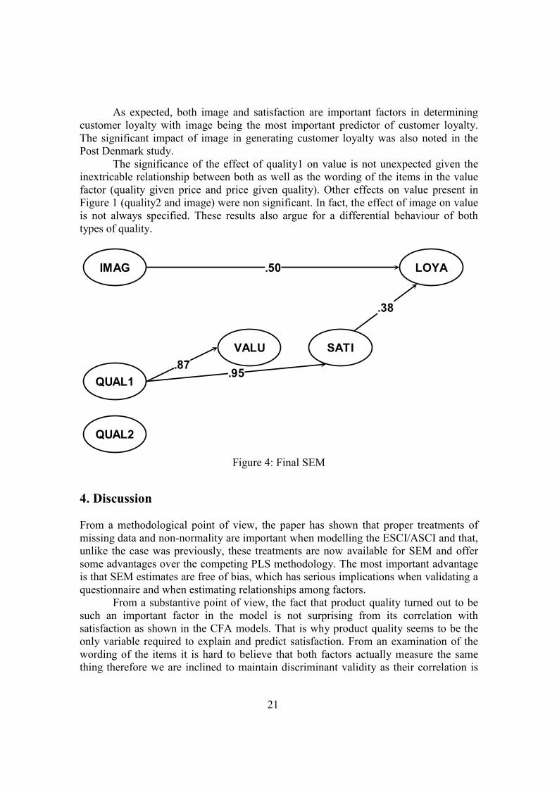
The final model indicates that the main and only driver of consumer satisfactionis the quality of the Post Office products. Neither service quality nor value, nor imagehave a significant impact on satisfaction levels. In fact, the quality of the Post Officecustomer service or “humanware” appears to have no significant impact on any of thefactors in the model. Thus, similar to Post Denmark (Kristensen et al., 1999) thedelineation between service and product quality is necessary.

21

As expected, both image and satisfaction are important factors in determiningcustomer loyalty with image being the most important predictor of customer loyalty.The significant impact of image in generating customer loyalty was also noted in thePost Denmark study.

The significance of the effect of quality1 on value is not unexpected given theinextricable relationship between both as well as the wording of the items in the valuefactor (quality given price and price given quality). Other effects on value present inFigure 1 (quality2 and image) were non significant. In fact, the effect of image on valueis not always specified. These results also argue for a differential behaviour of bothtypes of quality.

IMAG

QUAL1

QUAL2

VALU SATI

LOYA.50

.38

.95.87

Figure 4: Final SEM

4. Discussion

From a methodological point of view, the paper has shown that proper treatments ofmissing data and non-normality are important when modelling the ESCI/ASCI and that,unlike the case was previously, these treatments are now available for SEM and offersome advantages over the competing PLS methodology. The most important advantageis that SEM estimates are free of bias, which has serious implications when validating aquestionnaire and when estimating relationships among factors.

From a substantive point of view, the fact that product quality turned out to besuch an important factor in the model is not surprising from its correlation withsatisfaction as shown in the CFA models. That is why product quality seems to be theonly variable required to explain and predict satisfaction. From an examination of thewording of the items it is hard to believe that both factors actually measure the samething therefore we are inclined to maintain discriminant validity as their correlation is

22

significantly different from 1, even if only by a narrow margin. There is ample evidencein the literature suggesting that perceived quality is the most significant predictor ofsatisfaction (e.g., Anderson & Sullivan, 1993; Churchill & Suprenant, 1982; Johnson &Fornell, 1991). However, Martensen et al., (2000) noted that the drivers of bothcustomer satisfaction and loyalty are in fact industry specific. For example theydemonstrated that image was the main driver of customer satisfaction in industries likecable Television, supermarkets and the internet. In contrast, satisfaction levels in thesoft drinks industry were driven by product quality. The distinction between servicequality and product quality proved justified in this analysis. In fact, service quality doesnot have a significant impact on value, satisfaction or loyalty. This result may bespecific to postal services or may have been caused by the high collinearity betweenproduct and service quality.

A very interesting, though not surprising result was the impact of image onloyalty. In fact image is the most important predictor of loyalty to the Isle of Man PostOffice. Satisfaction predicted loyalty to a lesser degree. A similar result wasdocumented by Kristensen et al., (1999) in relation to Post Denmark where image wasfound to be the most significant predictor of loyalty. Indeed this is a very importantobservation as competition within this segment of the market is going to increase in thefuture. Martensen et al., (2000) noted that in the fast food, internet and soft drinksindustries the main impact on loyalty comes from the product itself (product quality asopposed to service quality), whereas in more complex industries with more highlycompetitive markets (e.g., mobile phone industries) and industries with multiple outlets(e.g., supermarkets and Banks) loyalty is more image driven. Thus, the drivers ofcustomer loyalty are in fact industry specific. In this analysis both product and servicequality do not have a significant impact on loyalty. Martensen et al., (2000) argued thatloyalty was in fact the most significant outcome measure in the CSI model and was amore true measure of reality compared to satisfaction. They maintained that torecommend a product or service to others has greater consequences and requires morecommitment than just indicating that one is more or less satisfied compared to an idealor a competitive product or service.

In the CSI literature a more complex relationship between quality, value andsatisfaction is espoused. This relationship was partly realised in this analysis with onlyproduct quality having a significant impact on value. As quality is a major aspect of thevalue assessment, and given the definition of value this result is not surprising.However, because of the definitional interaction between quality and value Johnson etal., (2001) maintain that it is difficult to evaluate how much of the impact of quality onvalue is due to cause and effect and how much is true by definition. As such theysuggested replacing this factor in the model with a perceived price construct withcustomers evaluating price relative to a variety of benchmarks, including comparisonsof the product’s price versus expected price, competitors prices and quality, thusproducing a more pure price construct. In fact, the focus groups suggested that thewording of items in the value construct were confusing.

The fact that all factors are so highly correlated with all others raise two furtherpoints. Firstly, in a study like ours, where data are measurements obtained in a single

23

questionnaire, it is possible that correlations are artifactually inflated by what is knownas common method variance (See Linden & Whitney, 2001; Harrison et al., 1996).Secondly, statistically, there is an alternative way of structuring the relationships amongfactors when all factor correlations are high. That is to specify a higher order factorstructure between all the factors in the model. This model examines the communalitesbetween all factors implying that all are in fact measuring a global conceptualisation ofconsumer satisfaction. The intricate causal relationships (both direct and indirect)espoused in the ECSI/ACSI literature would thus be ignored. The fit of such a model toour data was nearly equally good to the fit of the model specifying causal relationshipsamong factors.

From a statistical point of view, using the data to modify the specification of themodel, as we have done, makes the results vulnerable to capitalization on chance(Luijben, 1989; MacCallum, 1986; MacCallum, 1995; MacCallum et al., 1992), a riskthat can only increase when collinearity is high. Some of the recommendations of theliterature to prevent capitalization on chance (make only one modification at a time, useboth the overall fit of the model and the significance of the individual parameters, maketheoretically sound modifications first) could be followed. Others could not. Our samplewas not large enough to spare a part of it for a crossvalidation exercise. However, someresults hint at the fact that the model modification was successful. We repeated themodification several times by removing different effects on the first step and the finalmodel was always the same. Along all this modification process, only one parametershifted from non significant to significant (the effect of satisfaction on loyalty) all therest were either always significant or always non-significant.

References

Aburckle, J. L. (1996), Full Information Estimation in the Presence of IncompleteData, in Marcoulides, G.A. and Schumacker, R.E. (eds.), Advanced Structural EquationModeling, Mahwah, NJ, Erlbaum, (pp. 243-277).

Aburckle, J. L. and Wothke, W. (1999), Amos (Version 4.0), Chicago, IL,Smallwaters.

Allison, P. D. (1987), Estimation of Linear Models with Incomplete Data, inClogg, C.C. (ed.), Sociological Methodology, 1987, Washington DC, AmericanSociological Association, (pp. 71-103).

American Society for Quality (1998), American Customer Satisfaction Index(ACSI) Methodology Report, Ann Arbor, Mi: Arthur Andersen, University of Michigan.

Anderson, E.W. and Fornell, C. (2000), Foundations of the American CustomerSatisfaction Index, Total Quality Management 11, S869-S882.

Anderson, E.W., Fornell, C. and Lehrmann, D.R. (1994), Customer Satisfaction,Market Share, and Profitability: Findings from Sweden. Journal of Marketing 58, 53-66.

24

Anderson, E. W. and Sullivan, M. (1993), The Antecedents and Consequences ofCustomer Satisfaction for Firms, Marketing Science 12, 125-143.

Andreassen, T. W. and Lindestad, B. (1998a), The Effects of Corporate Image inthe Formation of Customer Loyalty, Journal of Service Marketing 1, 82-92.

Andreassen, T. W. and Lindestad, B. (1998b), Customer Loyalty and ComplexServices, the Impact of Corporate Image on Quality, Customer Satisfaction and Loyaltyfor Customers with Varying Degrees of Service Expertise, International Journal ofService Industry Management 9, 7-23.

Arminger, G. and Sobel, M. E. (1990), Pseudo Maximum Likelihood Estimationof Mean and Covariance Structures with Missing Data, Journal of the AmericanStatistical Association 85, 195-203.

Barnett, V. and Lewis, T. (1994), Outliers in Statistical Data, New York, Wiley.Batista-Foguet, J. M. and Coenders, G. (1998), Introducción a los Modelos

Estructurales. Utilización del Análisis Factorial Confirmatorio para la Depuración de unCuestionario [Introduction to Structural Equation Models. Using a Confirmatory FactorAnalysis Model to Improve a Questionnaire], in Renom, J. (ed.) TratamientoInformatizado de Datos [Computer Data Analysis], Barcelona, Masson, (pp. 229-286).

Batista-Foguet, J. M. and Coenders, G. (2000), Modelos de EcuacionesEstructurales [Structural Equation Models], Madrid, La Muralla.

Bentler, P.M. (2000), EQS 6.0, Encino, CA, Multivariate Software.Bollen, K. A. (1989), Structural Equations with Latent Variables, New York,

Wiley.Bollen, K.A. and Long, J.S. (1993), Testing Structural Equation Models.

Newbury Park, Ca, Sage.Browne, M.W. (1984), Asymptotically Distribution-Free Methods for the

Analysis of Covariance Structures, British Journal of Mathematical and StatisticalPsychology 37, 62-83.

Cassel, C., Hackl, P. and Westlund, A.H. (2000), On Measurement of TangibleAssets, a Study of Robustness of Partial Least Squares, Total Quality Management 11,897-907.

Churchill, G. A., and Suprenant, C. (1982), An Investigation Into theDeterminants of Consumer Satisfaction, Journal of Marketing Research 19, 491-504.

Coenders, G. and Saris, W. E. (1995), Categorization and Measurement Quality.The Choice Between Pearson and Polychoric Correlations, in Saris, W.E. and Münnich,Á., (eds.), The Multitrait-Multimethod Approach to Evaluate Measurement Instruments,Budapest, Eötvös University Press, (pp. 125-144).

Coenders, G., and Saris, W. E. (2000), Testing Nested Additive, Multiplicativeand General Multitrait-Multimethod Models, Structural Equation Modeling 7, 219-250.

Coenders, G., Satorra, A. and Saris, W. E. (1997), Alternative Approaches ToStructural Modeling of Ordinal Data, a Monte Carlo Study, Structural Equation Modeling4, 261-282.

Dijkstra, T. (1983), Some Comments on Maximum Likelihood and Partial LeastSquares Methods, Journal of Econometrics 22, 67-90.

25

ECSI Technical Committee (1998), European Customer Satisfaction Index,Foundation and Structure for Harmonized National Pilot Projects. Report Prepared forthe ECSI Steering Committee, October.

Eklöf, J. A. (2000), European Customer Satisfaction Index Pan-EuropeanTelecommunication Sector Report Based on the Pilot Studies 1999. Stockholm, Sweden,European Organization for Quality and European Foundation forQuality Management.

Enders, C.K. (2001), The Impact of Non-Normality on Full InformationMaximum Likelihood Estimation for Structural Equation Models with Missing Data,Psychological Methods 6, 352-370.

Enders, C.K. and Bandalos, D.L. (2001), The Relative Performance of FullInformation Maximum Likelihood Estimation for Missing Data in Structural EquationModels, Structural Equation Modeling 8, 430-457.

Fornell, C. (1992), A National Customer Satisfaction Barometer, the SwedishExperience, Journal of Marketing 56, 6-21.

Fornell, C. and Cha, J. (1994), Partial Least Squares, in Bagozzi, R.P., (ed.),Advanced Methods in Marketing Research, Cambridge, Basil Blackwell, (pp. 52-78).

Fornell, C., Johnson, M. D., Anderson, E. W., Cha, J., and Bryant, B. E. (1996),The American Customer Satisfaction Index, Nature, Purpose and Findings, Journal ofMarketing 60, 7-18.

Fouladi, R.T. (2000), Performance of Modified Test Statistics in Covariance andCorrelation Structure Analysis under Conditions of Multivariate Non-Normality,Structural Equation Modeling 7, 356-410.

Graham, J.W., Hofer, S.M. and Mackinnon, D.P. (1996), Maximizing theUsefulness of Data Obtained with Planned Missing Data Patterns, an Application ofMaximum Likelihood Procedures, Multivariate Behavioral Research 31, 197-218.

Graham, J.W., Hofer, S.M. and Piccinin, A.M. (1994), Analysis with Missing Datain Drug Prevention Research, in Collins, L.M. and Seitz, L., (eds.), Advances in DataAnalysis for Prevention Intervention Research, Washington, DC, National Institute onDrug Abuse, (pp. 13-63).

Graham, J.W., Taylor, B.J. and Cumsille, P.E. (2001), Planned Missing DataDesigns in the Analysis of Change, in Collins, L.M. and Sayer, A., (eds.), New Methodsfor the Analysis of Change, Washington, DC, APA., (pp. 333-354).

Groves, R. M. (1989), Survey Errors and Survey Costs. New York: John Wiley &Sons.

Hackl, P., Scharitzer, D. and Zuba, R. (2000), Customer Satisfaction in theAustrian Food Retail Market, Total Quality Management 11, 999-1006.

Harrison, D. A., McLaughlin, M. E. and Coalter, T. M. (1996), Context,Cognition, and Common Method Variance: Psychometric and Verbal ProtocolEvidence, Organizational Behavior and Human Decision Processes 68, 246-261.

Howard, J. A. and Sheth, J. N. (1969), The Theory of Buyer Behavior, New York,Wiley.

26

Johnson, M.D. and Fornell, C. (1991), A Freamework for Comparing CustomerSatisfaction across Individuals and Product Categories, Journal of EconomicPsychology 12, 267-286.

Johnson, M. D., Gustafsson, A., Andreassen, T. W., Lervik, L. and Cha, J. (2001),The Evolution and Future of National Customer Satisfaction Index Models, Journal ofEconomic Psychology 22, 217-245.

Jöreskog, K. G. (1973), A General Method for Estimating a Linear StructuralEquation System, in Goldberger, A.S. and Duncan, O.D. (eds.), Structural EquationModels in the Social Sciences, New York, Academic Press, (pp. 85-112).

Jöreskog, K. G. (1990), New Developments in LISREL. Analysis of OrdinalVariables Using Polychoric Correlations and Weighted Least Squares, Quality andQuantity 24, 387-404.

Jöreskog, K. G. and Sörbom, D. (1993), New Features in PRELIS2, Chicago, IL,Scientific Software International.

Jöreskog, K. G, Sörbom, D., Du Toit, S., and Du Toit, M. (2000), LISREL 8, NewStatistical Features (Rev.), Chicago, IL, Scientific Software International.

Kristensen, K., Martensen, A. and Grønholdt, L. (1999), Measuring the Impact ofBuying Behaviour on Customer Satisfaction, Total Quality Management 10, 602-614.

Linden, M. K. and Whitney, D. J. (2001), Accounting for Common MethodVariance in Cross-Sectional Research Designs, Journal of Applied Psych 86, 114-121.

Little, R.J.A. and Rubin, D.B. (1987), Statistical Analysis with Missing Data, NewYork, Wiley.

Luijben, T. (1989), Statistical Guidance for Model Modification in CovarianceStructure Analysis, Amsterdam, Sociometric Research Foundation.

Maccallum, R.C. (1986), Specification Searches in Covariance StructureModeling, Psychological Bulletin 100, 107-120.

Maccallum, R.C. (1995), Model Specifiaction, Procedures, Strategies and RelatedIssues, in Hoyle, R.H. (ed.), Sructural Equation Modeling. Concepts, Issues andApplications, Thousand Oaks, CA, Sage, (pp. 16-36).

Maccallum, R.C., Roznowski, M. and Necowitz, L.B. (1992), Model Modificationin Covariance Structure Analysis, the Problem of Capitalization on Chance,Psychological Bulletin 111, 490-504.

Mahalanobis, P. (1936), On the Generalized Distance in Statistics, Proceedings ofthe National Institute of Science, Calcutta, 12, 49-55.

Martensen, A., Grønholdt, L. and Kristensen, K. (2000), The Drivers of CustomerSatisfaction and Loyalty, Cross-Industry Findings From Denmark, Total QualityManagement 11, 8544-8553.

Muthén, B. (1984), A General Structural Equation Model with Dichotomous,Ordered Categorical and Continuous Latent Variable Indicators. Psychometrika 43, 241-250.

Muthén, B. (1994), Multilevel Covariance Structure Analysis, Sociological Methodsand Research 22, 376-398.

Muthén, B. (2001), Second-Generation Structural Equation Modeling with aCombination of Categorical and Continuous Latent Variables, New Opportunities for

27

Latent Class/Latent Growth Modeling, in Collins, L.M. and Sayer, A., (eds.), NewMethods for the Analysis of Change, Washington, DC, APA, (pp. 291-322).

Muthén, B. and Kaplan, D. (1989), A Comparison of Some Methodologies for theFactor Analysis of Non-Normal Likert Variables. A Note on the Size of the Model, BritishJournal of Mathematical and Statistical Psychology 45, 19-30.

Muthén B., Kaplan, D. and Hollis. M. (1987), On Structural Equation Modelingwith Data that Are not Missing Completely at Random, Psychometrika 52, 431-462.

Muthén, B. and Satorra, A. (1995), Complex Sample Data in Structural EquationModeling, Sociological Methodology 25, 267-316.

Muthén, L. K. and Muthén, B. (2001), Mplus User’s Guide. Los Angeles, CA,Muthén and Muthén.

Neale, M. C., Boker, S.M., Xie, G. and Maes, H. H. (1999), Mx, StatisticalModeling. 5th Edition, Box 126, MCV, Richmond, VA23298, Department of Psychiatry.

Nevitt, J. and Hancock, G. R. (2001), Performance of Bootstrapping Approaches toModel Test Ststaistics and Parameter Standard Error Estimation in Structural EquationModelling, Structural Equation Modeling 8, 353-377.

Raykov, T. and Marcoulides, G.A. (2000), A First Course in Structural EquationModeling, Mahwah, NJ, Lawrence Erlbaum.

Reichheld, F.F. and Sasser, W.E. (1990), Zero Defections, Quality Comes toServices, Harvard Business Review 68, 105-111.

Rubin, D. B. (1987), Multiple Imputation for Nonresponse in Surveys, New York,Wiley.

Satorra, A. (1990), Robustness Issues in Structural Equation Modeling, a Review ofRecent Developments, Quality and Quantity 24, 367-86.

Satorra, A. (1992), Asymptotic Robust Inferences in the Analysis of Mean andCovariance Structures, in Marsden, P.V., (ed.), Sociological Methodology 1992,Cambridge, Basil Blackwell, (pp. 249-278).

Satorra, A. (1993), Asymptotic Robust Inferences in Multi-Sample Analysis ofAugmented-Moment Matrices, in Rao, C.R. and Cuadras, C.M., (eds.), MultivariateAnalysis, Future Directions 2, Amsterdam, North-Holland, (pp. 211-229).

Satorra, A. and Bentler, P.M. (1994), Corrections to Test Statistics and StandardErrors in Covariance Structure Analysis, in Von Eye, A. and Clogg, C., (eds.), LatentVariables Analysis, Applications to Developmental Research, Thousand Oaks, Ca, Sage,(pp. 399-419).

Satorra, A. and Bentler, P.M. (1999), A Scaled Difference Chi-Square Test Statisticfor Moment Structure Analysis, Technical Report. University of California, Los Angeles.

Du Toit, M., and du Toit, S., (2001), Interactive LISREL, User's Guide, Chicago,IL, Scientific Software International.

Widaman, K. (1993), Common Factor Analysis versus Principal ComponentAnalysis, Differential Bias in Representing Model Parameters?, Multivariate BehavioralResearch 25, 1-28.

Wold, H. (1975), Path Models with Latent Variables, the NIPALS Approach, inBlalock, H.M., Aganbegian, A., Borodkin, F.M., Boudon, R. and Cappecchi, V., (eds.),

28

Quantitative Sociology. International Perspectives on Mathematical and StatisticalModeling, New York, Academic Press, (pp. 307-353).

Wothke, W. (2000), Longitudinal and Multi-Group Modeling with Missing Data.in Little, T.D., Schnabel, K.U. and Baumert, J., (eds.), Modeling Longitudinal andMultilevel Data, Practical Issues, Applied Approaches and Specific Examples, Mahwah,NJ, Lawrence Erlbaum, (pp. 219-240).

Yuan, K.-H., and Bentler, P.M. (2000), Three Likelihood-Based Methods forMean and Covariance Structure Analysis with Nonnormal Missing Data, in Sobel, M.E.and Becker, M.P., (eds.), Sociological Methodology 2000, Washington, DC, AmericanSociological Association, (pp. 165-200).

application of the european customer satisfaction index … · 1 application of the european...

Documents