appendix g:ecohydraulics specialist report. appendix g... · appendix g:ecohydraulics specialist...

ESIA of the Gulpur Hydropower Project

Hagler Bailly Pakistan Appendix G R4V07GHP: 09/23/14 G-1

Appendix G: Ecohydraulics Specialist Report

See following pages.

i

GULPUR HYDROPOWER PLANT

ENVIRONMENTAL FLOW ASSESSMENT

ECOHYDRAULICS SPECIALIST REPORT

A. Birkhead, Streamflow Solutions

March 2013

Table of Contents

Table of Contents .............................................................................................................................................. i

List of Figures ................................................................................................................................................. iii

List of Tables .................................................................................................................................................. iv

Abbreviations and Acronyms ....................................................................................................................... v

Acknowledgements ....................................................................................................................................... vi

1 Introduction .............................................................................................................................. 7

2 Topographic and hydraulic data ........................................................................................... 8

2.1 Topographic data ..................................................................................................................... 8

2.2 Hydraulic data ....................................................................................................................... 15

2.2.1 Stage measurements ................................................................................................................. 15

2.2.2 Discharge measurements .......................................................................................................... 15

2.2.2.1 Manual gauging ....................................................................................................................... 15

2.2.2.2 Rehman Bridge Gauge .............................................................................................................. 16

3 Hydraulic analysis and modelling ...................................................................................... 17

3.1 HECRAS modelling............................................................................................................... 17

3.1.1 Model set-up and calibration .................................................................................................... 18

3.1.2 Model application ..................................................................................................................... 20

3.2 Hydraulic characterisation for use in the DRIFT DSS ...................................................... 20

3.2.1 Hydraulic habitat-flow simulation modelling .......................................................................... 20

3.2.1.1 Model assumptions ................................................................................................................... 21

3.2.1.2 Data requirements .................................................................................................................... 21

4 Hydraulic results ................................................................................................................... 23

5 Hydrology............................................................................................................................... 25

5.1 Information supplied ............................................................................................................ 25

5.1.1 Historical flows ......................................................................................................................... 25

5.1.2 Dam and HPP layout: Option 1 .............................................................................................. 25

5.1.3 Baseload scenarios .................................................................................................................... 27

ii

5.2 Modelling of a peaking operational scenario .................................................................... 27

5.2.1 Operating rules ........................................................................................................................ 28

5.2.2 Results ...................................................................................................................................... 29

5.3 Results summary: peaking and baseload ........................................................................... 30

6 Updated layout for dam and HPP: Option 3 ..................................................................... 33

7 References ............................................................................................................................... 36

iii

List of Figures

Figure 2.1 Locality map showing the main rivers draining the Poonch River catchment.

Also indicated are the Gulpur HPP inlet, diversion tunnel and outlet (tailrace

outfall) for Layout Option 1, the location of EF sites, main towns and cities

(source: HBP) .............................................................................................................................9

Figure 2.2 The positioning of surveyed cross-sections at EF Site 1 (Kallar Bridge) using a 15

March 2010 aerial view. ..........................................................................................................10

Figure 2.3 Composite photographs of the Poonch River at EF Site 1, taken from the position

indicated in Figure 2.2 (10 November 2013), showing cross-sections (10 and 11)

used for hydraulic characterisation in the DRIFT DSS. .....................................................10

Figure 2.4 The positioning of surveyed cross-sections at EF Site 2 (Borali Bridge) using a 1

November 2005 aerial view. ..................................................................................................11


indicated in Figure 2.4 (10 November 2013), showing cross-sections (1 and 3) used

for hydraulic characterisation in the DRIFT DSS. ..............................................................11

Figure 2.6 The positioning of surveyed cross-sections at EF Site 3 (Gulpur Bridge) using a 1

November 2005 aerial view. ..................................................................................................12

Figure 2.7 Composite photographs of the Poonch River at EF Site 3, taken from the positions



Figure 2.8 The positioning of surveyed cross-sections at EF Site 4 (Billiporian Bridge) using a

9 February 2013 aerial view. ..................................................................................................13




Figure 2.10 Plots of selected cross-section profiles: top-left: EF Site 1 (cross-section 10), top-

right: EF Site 2 (cross-section 1), bottom-left: EF Site 3 (cross-section 1), bottom-

right: EF Site 4 (cross-section 3) .............................................................................................14

Figure 2.11 Photographs of the Rehman Bridge Gauging Station, located c. 130 m below the

confluence of the Poonch River and Ban Nullah. Note the 1992 High Flood Level

(HFL) of 1740 ft amsl (source: Mr Yasir Abbas, NESPAK) ...............................................17

Figure 3.1 Plots of the longitudinal bed slope, surveyed stages (21 to 24 October 2013) and

modelled water surface profiles for the four EF sites (top-left: EF Site 1, 17.2 m3 s-1;

top-right: EF Site 2, 37.9 m3 s-1; bottom-left: EF Site 3, 40.0 m3 s-1; bottom-right: EF

Site 4 , 49.2 m3 s-1). ...................................................................................................................19

Figure 4.1 Modelled rating (stage vs. discharge) relationships for EF site.cross-sections 1.10

(top-left), 2.1(top-right), 3.1 (bottom-left) and 4.3 (bottom-right) ....................................22

Figure 5.1 Francis and Kaplan (adjustable guide vanes) turbine efficiency curves used to

compute power generation. The efficiency for the Francis turbine is limited to a

discharge ratio of 0.5 to provide at least 72.5% efficiency; for the Kaplan turbine

the minimum ratio is 0.20 (78.0%) (source: SKAT, 1985) ...................................................28

iv

Figure 5.2 Discharge time series for the period 1 July to 30 September 2011, showing the

Baseline (historical) average daily flows at EF Site 3 (red) and that resulting from

peaking Scenario G8Peak (blue) (cms = m3 s-1) ...................................................................29

Figure 6.1 The dewatered section of the Poonch River between the proposed Gulpur Dam

Site and tailrace outfall (Option 3), using a 1 November 2005 (low flow) aerial

view. ..........................................................................................................................................35

Figure 6.2 Discharge time series for the period 1 January 2010 to 31 December 2011, showing

the Baseline (historical) average daily flows at EF Site 2 (red) and those resulting

from Baseload Scenario G8OR (blue) (cms = m3 s-1) ..........................................................35

List of Tables

Table 2.1 Geographic site positions and dates of river topographic surveys ...................................9

Table 2.2 Stage and discharge data for EF Site 1 .................................................................................15




Table 3.1 Calibrated reach-averaged flow resistance coefficients .....................................................18

Table 3.2 Regression coefficients in the rating relationship given by Equation 3.1 .......................23

Table 4.1 Example (EF Site 2.1) of the text file output from HABFLO used in the DRIFT DSS ...23

Table 5.1 Catchment-area factors for the EF sites................................................................................25

Table 5.2 Selected design features for the dam and HPP: Layout Option 1 ....................................25

Table 5.3 Option 1: dam level - storage volume - surface area..........................................................26

Table 5.4 Monthly average evaporation ...............................................................................................26

Table 5.5 Annual water balance for Scenario G8Peak ........................................................................29

Table 5.6 Summary showing the influence of EF release on average annual power

generation and reduction relative to no EF for baseload and peaking operation

(Layout Option 1: MAR= 3965.2 106 m3, Layout Option 3: MAR = 3989.0 106 m3) .........31

Table 6.1 Selected design features for the dam and HPP: Layout Option 3 ....................................33

Table 6.2 Option 3: dam level - storage volume - surface area..........................................................33

v

Abbreviations and Acronyms

amsl above mean sea level

dec. deg. decimal degrees

Baseline Historical hydrology: 1960 to 2011

DRIFT Downstream Response to Imposed Flow Transformation

DSL Dead Storage Level

DSS Decision Support System

EF Environmental Flow

ft feet

GE Google Earth

GIS Geographic Information System

GWha-1 Giga Watt-hours per annum

HBP Hagler Bailly Pakistan

HECRAS Hydrological Engineering Centre River Analysis System

HPP Hydropower Plant

LOC Line of Control

mamsl meters above mean sea level

MAR Mean Annual Runoff

MOL Minimum Operating Level

MWL Maximum Water Level

MS Microsoft

m3 s-1 cubic meters per second

NESPAK National Engineering Services Pakistan (Pvt.) Limited

NOL Normal Operating Level

SKAT Swiss Centre for Appropriate Technology

SPD Survey of Pakistan Datum

WGS 84 World Geodetic System 1984

WWF World Wildlife Fund

vi

Acknowledgements

The topographic survey and manual flow gauging data used in this study were collected by

STECO and the World Wildlife Fund (WWF). River surveys in this environment, characterised

by fast flows over steep rapids, are challenging, even in the low flow season, and the teams

responsible for the data collection are gratefully acknowledged. Hagler Bailey Pakistan (HBP)

was responsible for overseeing the river site surveys, and the efforts of Mr Vaqar Zakaria and Mr

Hussain Ali in this regard are much appreciated.

7

1 INTRODUCTION

This report describes the topographic and hydraulic data (Section 2); analysis and modelling

(Section 3); and hydraulic results (Section 4) for the proposed Gulpur Hydropower Plant

(HPP) EF Sites 1 (Kallar Bridge), 2 (Borali Bridge), 3 (Gulpur Bridge) and 4 (Billiporian

Bridge) on the Poonch River in Kashmir, Pakistan. The locations of the EF Sites 1 to 4 are

shown in the locality map in Figure 2.1, together with the diversion tunnel for Layout Option

1.1 The proposed weir site is located c. 200 to 500 m downstream of the Ban Nullah

confluence. Hydrological information and HPP scenario modelling are discussed in Sections

5 and 0.

Additional details on the river, the EF assessment and the Gulpur HPP project are available

in HBP (2014).

1 Changes to the Gulpur HPP layout occurred after the EF site selection (10.10.2013), and was not finalised prior to the

hydraulic/hydrological analysis and modelling being completed (03.12.2013). An updated layout for the HPP (Option 3) and baseload operational rules (12.03.2014) are presented in Section 0.

8

2 TOPOGRAPHIC AND HYDRAULIC DATA

2.1 TOPOGRAPHIC DATA

Requirements for the topographic river surveys (and hydraulic data collection - refer to

Section 2.2, following) were communicated to Hagler Bailey Pakistan (HBP) on 10 October

2013. These included a written explanation of the data collection requirements and location

of cross-sections at the EF sites.

The following were provided:

1. Google Earth (GE) file with EF site and cross-section locations;

2. GE images of 1. above (per site), using the historical image with the lowest flow;

3. Geographic Information System (GIS) shape files;

4. Microsoft (MS) Excel file providing the end positions per cross-section as extracted

from the GE file (1. above), geomorphological units through which the cross-sections

are located and descriptions thereof;

5. MS Powerpoint file providing identifiers showing the (approximate) cross-section

locations on selected photographs (supplied by HBP) that could be reconciled with

the GE views and preferred cross-section positioning.

Surveys were done by World Wildlife Fund (WWF) and STECO, under the auspices of HBP.

At EF Site 1, 11 linked cross-sections were surveyed over a reach distance of 764 m; at EF Site

2, six linked cross-sections were surveyed over a reach distance of 998 m; at EF Site 3, seven

linked cross-sections were surveyed over a reach distance of 705 m; at EF Site 4, five linked

cross-sections were surveyed over a reach distance of 387 m. The geographic site positions

and survey dates are provided in Table 2.1 for these four sites.

9

Table 2.1 Geographic site positions and dates of river topographic surveys

EF site Location (dec. deg., WGS 84) Topographic survey

dates Number Name Latitude (E) Longitude (N)

1 Kallar Bridge 73.934733 33.578836 21 - 22.10.2013

2 Borali Bridge 73.869342 33.472497 22 - 23.10.2013

3 Gulpur Bridge 73.837169 33.449514 23.10.2013

4 Billiporian Bridge 73.790117 33.383314 24.10.2013

Figure 2.1 Locality map showing the main rivers draining the Poonch River catchment. Also

indicated are the Gulpur HPP inlet, diversion tunnel and outlet (tailrace outfall) for

Layout Option 1, the location of EF sites, main towns and cities (source: HBP)

Aerial photographs showing the locations of cross-sections surveyed at the EF sites, and

ground photographs (that show selected cross-sections) are provided in Figure 2.2 to Figure

10

2.9. Survey data were provided (by STECO) in the form of Eastings and Northings 2, with

elevations relative to the Survey of Pakistan Datum (SPD).

7

65

4

3

2

9

8

1

Figure 2.3 view

100 m

Flow

N

1011

Figure 2.2 The positioning of surveyed cross-sections at EF Site 1 (Kallar Bridge) using a 15

March 2010 aerial view.

11

10



for hydraulic characterisation in the DRIFT DSS.

2 As far as could be established, the projection used was Kalianpur 1962/India zone I.

11

5

4

3

2

1

6

Figure 2.5 view

100 m

Flow

N

Figure 2.4 The positioning of surveyed cross-sections at EF Site 2 (Borali Bridge) using a 1

November 2005 aerial view.

2

1

3

4




12

76

5

4

3

2

1100 m

Flow

N

Figure 2.7 views

Figure 2.6 The positioning of surveyed cross-sections at EF Site 3 (Gulpur Bridge) using a 1

November 2005 aerial view.

21

3

Figure 2.7 Composite photographs of the Poonch River at EF Site 3, taken from the positions



13

5

4

3

2

1

100 m

Flow

N

Figure 2.9 view

Figure 2.8 The positioning of surveyed cross-sections at EF Site 4 (Billiporian Bridge) using a

9 February 2013 aerial view.

2

1

3 4 5


indicated in Figure 2.8 (9 November 2013), showing cross-sections (3 and 5) used for

hydraulic characterisation in the DRIFT DSS.

The above water channel topography (at the time of data collection) was surveyed by

standard land surveying methods. For non-wadeable conditions, the channel bed was

surveyed using sonar. Depth sounding took place by mounting the sonar equipment on a

float and attaching to a tag line. The cross-sections used to derive hydraulic information for

use in the DRIFT DSS are plotted in Figure 2.10.

14

615

620

625

630

635

640

645

0 20 40 60 80 100 120 140 160

Ele

va

tio

n (m

am

sl)

Distance across channel (m)

487

488

489

490

491

492

493

494

495

496

0 10 20 30 40 50 60 70 80 90 100

Ele

va

tio

n (m

am

sl)


451

452

453

454

455

456

457

458

459

460

461

0 20 40 60 80 100 120 140

Ele

va

tio

n (m

am

sl)


384

386

388

390

392

394

396

398

400

402

0 50 100 150 200 250

Ele

va

tio

n (m

am

sl)


Figure 2.10 Plots of selected cross-section profiles: top-left: EF Site 1 (cross-section 10), top-right: EF Site 2 (cross-section 1), bottom-left: EF Site 3 (cross-

section 1), bottom-right: EF Site 4 (cross-section 3)

15

2.2 HYDRAULIC DATA

2.2.1 Stage measurements

Stage measurements were made on the right and left banks of the surveyed cross-sections at

the time of topographic surveys (Table 2.1), and these data are included in Error! Not a valid

bookmark self-reference. to Table 2.5. Also included are the approximate (surveyed) stages

corresponding to historic high flows and floods, including: high flows during the previous

wet season, and the 2010 (EF Site 1) and 1992 (all EF sites) floods. These stage measurements

are valuable for calibrating the hydraulic models for high flows, particularly for this study

where only a single set of directly measured low flow rating (stage-discharge) data are

available.

2.2.2 Discharge measurements

Discharge measurements were provided by manual gauging and also by making use of

measurements from the Rehman Bridge Gauge on the Poonch River at Kotli (refer to Section

2.2.2.2).

2.2.2.1 Manual gauging

Manual gauging was performed using an acoustic doppler profiler, held in position along

the transect using a tag line. The velocity-area method (BS 3680) was used for discharge

computation.

The discharges measured at the four EF sites were 17.2, 37.9, 40.0 and 49.2 m3 s-1,

respectively.

Table 2.2 Stage and discharge data for EF Site 1

EF Site 1

Date 21.10.2013 14.08.2013 28.07.2010 10.09.1992

Discharge (m3 s-1) 17.2 476 995 3060

Cross-section Stage (mamsl)

1 618.71 622.20 623.36

2 618.90 620.56 621.78 622.70

3 619.02 620.53 621.85 623.32

4 619.54 627.48 630.22

5 620.26 625.73

6 620.75 623.26 625.93

7 620.99 624.94 628.70

8 621.13 624.93

9 621.38 624.42 626.01

10 624.38 626.53 627.32 629.07

113 624.45 627.68 629.33

3 Note: cross-section 11 was used directly in the DRIFT DSS (refer to Section 3.2)

16


EF Site 2

Date 23.10.2013 14.08.2013 28.07.2010 10.09.1992

Discharge (m3 s-1) 37.9 700 4500


14 489.56 491.17

2 489.65

3 490.07 493.92 495.78

4 490.75 495.68 498.31

5 491.65 495.70 498.81

6 492.52 496.21 499.56


EF Site 3

Date 24.10.2013 14.08.2013 28.07.2010 10.09.1992

Discharge (m3 s-1) 40.0 700 4500


15 452.82 455.59 458.72

2 453.61 455.26 460.29

3 453.60 456.65 458.81

4 453.48 456.03 458.34

5 453.69 455.02 458.97

6 455.46 459.17 464.59

7 455.97


EF Site 4

Date 25.10.2013 14.08.2013 28.07.2010 10.09.1992

Discharge (m3 s-1) 49.2 770 4950


1 385.09 388.53 395.79

2 385.91 388.73 393.62

36 387.59 390.51 396.52

4 387.85 391.44 394.64

5 387.96 391.83 396.06

2.2.2.2 Rehman Bridge Gauge

Records from the Rehman Bridge Gauge on the Poonch River at Kotli, located c. 130 m

downstream of its confluence with the Ban Nullah, were used to provide the maximum

discharge for the wet season prior to the survey in October 2013, and historic floods7 in 2010




7 Historic maximum flood discharges and their corresponding surveyed stage levels (Hydraulic data

17

and 1992 (refer to Figure 2.11).

These stage and discharge data have been used to develop hydraulic models for each of the

sites, which are described in Section 3, following.

1.1.1 Stage measurements

Stage measurements were made on the right and left banks of the surveyed cross-sections at

the time of topographic surveys (Table 2.1), and these data are included in Error! Not a valid

bookmark self-reference. to Table 2.5. Also included are the approximate (surveyed) stages

corresponding to historic high flows and floods, including: high flows during the previous

wet season, and the 2010 (EF Site 1) and 1992 (all EF sites) floods. These stage measurements

are valuable for calibrating the hydraulic models for high flows, particularly for this study

where only a single set of directly measured low flow rating (stage-discharge) data are

available.

1.1.2 Discharge measurements

Discharge measurements were provided by manual gauging and also by making use of

measurements from the Rehman Bridge Gauge on the Poonch River at Kotli (refer to Section

2.2.2.2).

1.1.2.1 Manual gauging

Manual gauging was performed using an acoustic doppler profiler, held in position along

the transect using a tag line. The velocity-area method (BS 3680) was used for discharge

computation.

The discharges measured at the four EF sites were 17.2, 37.9, 40.0 and 49.2 m3 s-1,

respectively.

Table 2.2 to Table 2.5) were used circumspectly, since it is not unreasonable to expect that subsequent physical channel changes have occurred, and furthermore the stage levels are estimates (21 years ago for the 1992 flood)

18

Figure 2.11 Photographs of the Rehman Bridge Gauging Station, located c. 130 m below the

confluence of the Poonch River and Ban Nullah. Note the 1992 High Flood Level

(HFL) of 1740 ft amsl (source: Mr Yasir Abbas, NESPAK)

3 HYDRAULIC ANALYSIS AND MODELLING

3.1 HECRAS MODELLING

The well-known hydraulic modelling software, HECRAS (v4.1, available at

http://www.hec.usace.army.mil/) was used for steady-state non-uniform computations at

the EF sites.

The procedure used for setting-up and applying the hydraulic models was as follows:

calibration of flow resistance values (Manning's n is used in HECRAS) using the

stage-discharge (rating) data presented in Section 2.2, and

application of the models to interpolate and extrapolate the measurement-based

rating data.

3.1.1 Model set-up and calibration

For each of the sites, the georeferenced (refer to Figure 2.2 to Figure 2.9) topographic channel

cross-section data were imported into HECRAS. Reach lengths were measured using river

distances between cross-sections, and surveyed cross-sections were interpolated. Flow

resistances at high flows (floods) were determined using the surveyed flood stages, with

discharges estimated by the combination of recorded flows at the local gauging station8, the

8 approximately factored for upstream and downstream EF sites using catchment areas

19

need for flow continuity between sequential sites, and realistically calibrated resistance

values.

The Poonch River in the study area is characterised by pool-rapid channel type morphology,

with (less common) riffle features composed of cobbles. A typical hydraulic characteristic of

reaches with large-scale alluvial sediments (occurring in rapids) is increasing flow resistance

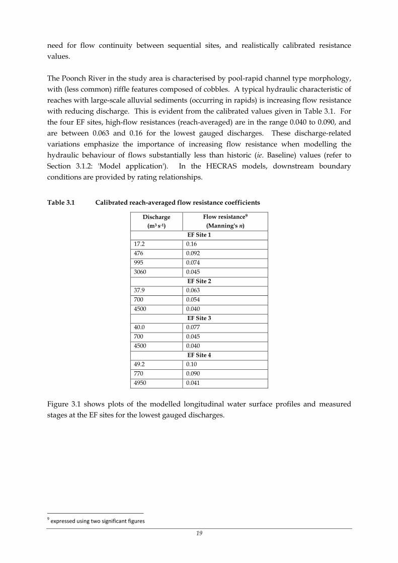
with reducing discharge. This is evident from the calibrated values given in Table 3.1. For

the four EF sites, high-flow resistances (reach-averaged) are in the range 0.040 to 0.090, and

are between 0.063 and 0.16 for the lowest gauged discharges. These discharge-related

variations emphasize the importance of increasing flow resistance when modelling the

hydraulic behaviour of flows substantially less than historic (ie. Baseline) values (refer to

Section 3.1.2: 'Model application'). In the HECRAS models, downstream boundary

conditions are provided by rating relationships.

Table 3.1 Calibrated reach-averaged flow resistance coefficients

Discharge

(m3 s-1)

Flow resistance9

(Manning's n)

EF Site 1

17.2 0.16

476 0.092

995 0.074

3060 0.045

EF Site 2

37.9 0.063

700 0.054

4500 0.040

EF Site 3

40.0 0.077

700 0.045

4500 0.040

EF Site 4

49.2 0.10

770 0.090

4950 0.041

Figure 3.1 shows plots of the modelled longitudinal water surface profiles and measured

stages at the EF sites for the lowest gauged discharges.

9 expressed using two significant figures

20

616

618

620

622

624

626

628

630

632

0 100 200 300 400 500 600 700

Sta

ge (

mam

sl)

Distance along the river (m)

Bed

Surveyed

HECRAS

486

488

490

492

494

0 200 400 600 800 1000

Sta

ge (

mam

sl)


Bed

Surveyed

HECRAS

448

450

452

454

456

458

0 100 200 300 400 500 600 700

Sta

ge (

mam

sl)


Bed

Surveyed

HECRAS

378

380

382

384

386

388

390

0 50 100 150 200 250 300 350

Sta

ge (

mam

sl)


Bed

Surveyed

HECRAS

Figure 3.1 Plots of the longitudinal bed slope, surveyed stages (21 to 24 October 2013) and modelled water surface profiles for the four EF sites (top-left:

EF Site 1, 17.2 m3 s-1; top-right: EF Site 2, 37.9 m3 s-1; bottom-left: EF Site 3, 40.0 m3 s-1; bottom-right: EF Site 4 , 49.2 m3 s-1).

21

3.1.2 Model application

In the application of the HECRAS models, hydraulic characteristics are computed for a range

of discharges. In the case of the Poonch River with Gulpur HPP operational, discharges in

the dry season will fall well below historic Baseline values10 along the dewatered reach

between the dam and tailrace outfall (represented by EF Site 2), and thus the flows used for

model calibrations in Section 3.1.1. Model applications are necessary to predict hydraulic

behaviour at these reduced flows, and it is consequently necessary to estimate concomitant

flow resistances. Low flow resistance values were extrapolated from the calibration values

(ie. as given in Table 3.1).

3.2 HYDRAULIC CHARACTERISATION FOR USE IN THE DRIFT DSS

3.2.1 Hydraulic habitat-flow simulation modelling

The (hydraulic) Habitat-Flow simulation model, HABFLO, was used to produce text files

relating discharge to ecologically relevant parameters, for use in the DRIFT DSS. The

hydraulic parameters included for (potential) use were maximum and average depth,

inundated width, wetted perimeter, average velocity, and a velocity-depth class relevant to

fish. The model is described in detail by Birkhead (2010).

Biota in the aquatic environment are associated with a combination of hydraulic variables

(eg. depth and velocity), as well as physical features such as substrate, vegetation and cover

for fish. Hydraulic habitat classes are a means of grouping these combinations into units

which have ecological meaning, in that they represent broad, known (or 'judged') preferences

of biota for hydraulic and biophysical variables. A class represents a range of values

pertaining to at least two environmental variables, of which at least one is flow-dependent

(depth, velocity, area of inundation, etc). Kleynhans (1999) suggested that the hydraulic

variables of depth-averaged velocity and depth, together with substrate and cover, may be

used to broadly characterise fish habitat. The environmental variables used (hydraulic and

biophysical) and their numerical ranges may be defined using available information on

conditions utilised by indicator biota that is available and relevant to the EF assessment.11

The abundance of hydraulic habitat defined by the combination of velocity and depth (ie. a

velocity-depth class) can be predicted by combining the result of a rating relationship (eg.

Equation 3.1) and the frequency-distribution of depth-averaged velocity (eg. Lamouroux et

al., 1995). For the Gulpur HPP EF assessment, response curves describing the abundance of

Mahaseer and Kashmir Catfish were directly linked to indicators of hydraulic habitat in the

DRIFT DSS. The flow preference is defined by a velocity-depth class with velocities in the

10

when flow is being diverted for power generation 11

For example, Lamouroux et al. (1999) developed regional habitat preferences for 24 fish species using five velocity classes. For rock catfish of the Senquyane River (southern Africa), Niehaus et al. (1997) found a velocity of 0.1 m s

-1 to be

the threshold separating recruits (lower values) from juveniles and adults (higher values). Cambray et al. (1989) noted that the fish species Barbus afer and Kneria auriculata spawn at depths of 0.1 - 0.2 m. Such data are ostensibly built into the preference ratings for fish species. Where detailed preference information exists (eg. Paxton, 2009) classes may be appropriately defined using suitable variables and resolutions.

22

range 0.1 - 0.7 m s-1, and depths in the range 0.25 - 0.50 m. The HABFLO model was used to

predict changes in the abundance of this class as a function of discharge, and the results are

expressed as available width on the cross-sectional profile (refer to Table 4.1).

3.2.1.1 Model assumptions

HABFLO is based on the assumptions that:

cross-sectional profiles and one-dimensional hydraulic parameters may be used to

characterise the bed topography and hydraulic conditions, respectively, in

morphological features,

frequency-distributions of depth-averaged velocity may be estimated with reasonable

accuracy using statistical methods, and

depth-averaged velocity and flow depth are mutually exclusive (ie. independent)

variables.

The use of cross-sections to represent characteristics (topographic and hydraulic) of

morphological features relates to their appropriate selection for EF assessment. Generally,

biotic considerations tend to dominate this selection, since hydraulic indicators of biotic

response to flow variation is of concern. However, while hydraulic considerations cannot

benefit from pre-eminence in the site selection process, they are important to the extent that

sites and sections chosen are not of such hydraulic complexity that reliable analysis and

prediction is impractical.

The reach-scale frequency-distribution velocity model of Lamouroux et al. (1995) provides

good predictions at the site scale, and fair predictions at the morphological feature scale

(Hirschowitz et al., 2007). Measurement of point depths and depth-averaged velocities in

rapids and riffles has indicated independence at low flows, where parameter estimation is

particularly relevant for EF assessment.

3.2.1.2 Data requirements

HABFLO model application requires the following data:

cross-sectional profile (ie. as plotted in Figure 2.10),

rating relationship (ie. as plotted in Figure 3.2),

numerical ranges defining velocity-depth classes, and

dominant roughness.

Rating relationships of the form given by Equation 3.1 were fitted (by regression) to the

modelled HECRAS rating data. The regression coefficients are provided in Table 3.2, and the

relationships are plotted in Figure 3.2 together with the HECRAS and measured data. The 'c'

coefficient in Equation 3.1 is the stage of zero discharge, and is the (maximum) stage

remaining (along the cross-section) when flow ceases.

23

623

624

625

626

627

628

629

630

631

1 10 100 1000

Sta

ge

(m

am

sl)

Discharge (m3 s-1)

Measured

HECRAS

Regression

488

489

490

491

492

493

494

495

496

497

1 10 100 1000

Sta

ge

(m

am

sl)

Discharge (m3 s-1)

Measured

HECRAS

Regression

451

452

453

454

455

456

457

458

459

460

1 10 100 1000

Sta

ge

(m

am

sl)

Discharge (m3 s-1)

Measured

HECRAS

Regression

386

388

390

392

394

396

398

1 10 100 1000

Sta

ge

(m

am

sl)

Discharge (m3 s-1)

Measured

HECRAS

Regression

Figure 3.2 Modelled rating (stage vs. discharge) relationships for EF site.cross-sections 1.10 (top-left), 2.1(top-right), 3.1 (bottom-left) and 4.3 (bottom-

right)

24

z = aQb + c

Equation 3.1

where z is stage (mamsl), Q is discharge (m3/s), and a, b and c are regression coefficients.

Table 3.2 Regression coefficients in the rating relationship given by Equation 3.1

Regression coefficients EF Site Cross-section

1.10 2.1 3.1 4.3

a 1.000 0.439 0.206 0.205

b 0.250 0.343 0.417 0.452

c 622.35 488.18 451.87 386.55

The dominant roughness is a parameter used in the frequency-distribution velocity

modelling, with values of 0.4 m for cross-sections through rapids used directly in the DRIFT

DSS.

4 HYDRAULIC RESULTS

The products of the analyses and modelling (Section 3) used to characterise hydraulic

conditions at the four EF sites are:

non-uniform hydraulic models in the form of HECRAS project files, and

text file outputs from HABFLO for use in the DRIFT DSS, an example of which is

provided in Table 4.1 for EF Site 2 (Borali Bridge).

Table 4.1 Example (EF Site 2.1) of the text file output from HABFLO used in the DRIFT DSS

Discharge

(m3 s-1)

Depth (m) Inundated

width (m)

Wetted

perimeter

(m)

Average

velocity

(m3 s-1)

Velocity-depth

class (m width) Maximum Average

0.0 0.15 0.09 18.8 18.8 0.00 0.0

0.1 0.20 0.13 20.9 20.9 0.03 0.0

0.2 0.25 0.17 22.3 22.3 0.05 0.1

0.3 0.30 0.21 23.6 23.6 0.06 2.1

0.5 0.35 0.24 25.0 25.0 0.08 4.3

0.7 0.40 0.28 26.2 26.2 0.10 7.0

1.0 0.45 0.32 27.1 27.2 0.12 9.2

1.4 0.50 0.35 28.9 29.0 0.14 10.6

1.8 0.55 0.37 31.0 31.0 0.16 8.1

2.4 0.60 0.40 33.0 33.1 0.18 6.3

3.0 0.65 0.42 35.1 35.2 0.20 4.7

3.7 0.70 0.45 37.1 37.2 0.22 4.0

4.6 0.75 0.49 38.3 38.4 0.25 4.1

5.5 0.80 0.53 38.8 39.0 0.27 5.0

6.6 0.85 0.57 39.4 39.5 0.30 5.5

7.8 0.90 0.61 40.0 40.1 0.32 6.0

9.2 0.95 0.64 41.6 41.7 0.35 6.8

10.7 1.00 0.62 46.2 46.4 0.37 6.2

12.4 1.05 0.63 49.2 49.4 0.40 5.2

25

Discharge

(m3 s-1)

Depth (m) Inundated

width (m)

Wetted

perimeter

(m)

Average

velocity

(m3 s-1)

Velocity-depth

class (m width) 14.2 1.10 0.66 50.8 51.0 0.42 4.3

16.2 1.15 0.70 51.6 51.8 0.45 3.4

18.3 1.20 0.74 52.3 52.5 0.47 3.4

20.6 1.25 0.78 53.1 53.3 0.50 5.1

23.2 1.30 0.81 54.6 54.8 0.53 6.5

25.9 1.35 0.83 56.7 56.9 0.55 6.8

28.8 1.40 0.85 58.5 58.8 0.58 6.7

31.9 1.45 0.89 59.5 59.7 0.61 5.2

35.3 1.50 0.92 60.5 60.7 0.63 3.7

38.8 1.55 0.96 61.3 61.5 0.66 3.3

42.6 1.60 1.00 62.0 62.3 0.69 2.8

46.6 1.65 1.04 62.7 63.0 0.72 2.8

50.9 1.70 1.07 63.5 63.7 0.75 3.2

55.4 1.75 1.11 64.2 64.5 0.78 3.2

60.2 1.80 1.15 64.9 65.2 0.81 2.6

65.2 1.85 1.18 65.7 66.0 0.84 2.0

70.5 1.90 1.22 66.4 66.7 0.87 1.6

76.1 1.95 1.26 67.1 67.4 0.90 1.5

82.0 2.00 1.29 67.8 68.2 0.93 1.4

88.1 2.05 1.33 68.6 68.9 0.97 1.1

94.6 2.10 1.37 69.1 69.5 1.00 1.1

101.3 2.15 1.41 69.4 69.8 1.03 1.1

108.4 2.20 1.46 69.7 70.1 1.07 1.0

115.7 2.25 1.50 70.0 70.4 1.10 1.0

123.4 2.30 1.54 70.3 70.8 1.14 0.7

131.5 2.35 1.59 70.6 71.1 1.17 0.8

139.8 2.40 1.63 70.9 71.4 1.21 0.6

148.5 2.45 1.67 71.2 71.7 1.25 0.4

26

5 HYDROLOGY

5.1 INFORMATION SUPPLIED

5.1.1 Historical flows

Historically gauged flows from the Rehman Bridge Station on the Poonch River at Kotli

(refer to Section 2.2.2.2) were supplied by Mira Power through HBP. These comprise the

Baseline hydrological data used in this study, and are for the period 1960 to 2011. The

Baseline discharge time series for the four EF sites were provided by the National

Engineering Services Pakistan Limited (NESPAK), and were estimated using proportional

catchment areas (Table 5.1).

Table 5.1 Catchment-area factors for the EF sites

EF site Catchment area factor

1 0.68

2 1.00

3 1.02

4 1.10

5.1.2 Dam and HPP layout: Option 1

Selected design features for the dam and HPP, relevant for modelling baseload and peaking

power generation scenarios, are listed in Table 5.2, with other pertinent information

including (Mira Power 2013):

dam level-storage volume-surface area (Table 5.3),

a power function for the tailwater rating relationship, which was determined by

regression using rating data provided (Equation 5.1),

monthly and annual average evaporation (Table 5.4), and

the head loss equation (Equation 5.2).

Table 5.2 Selected design features for the dam and HPP: Layout Option 1

Normal Operating Level (NOL) 540.0m

Number and type of turbines 3 x Francis

Total installed capacity 100 MW

Turbine efficiency 92.6%

River discharge at which generation ceases12 830 m3 s-1

12

To prevent damage to the turbines due to high suspended sediment loads.

27

Table 5.3 Option 1: dam level - storage volume - surface area

Level (mamsl) Storage (106 m3) Surface area (km2)

543.6MWL 32.131 3.121

540.0NOL 21.89 2.28

538.0MOL 17.72 1.89

535.0 12.78 1.40

530.0 7.17 0.87

525.0 3.72 0.52

520.0 1.62 0.32

517.0DSL 0.921 0.221

MWL: Maximum Water Level (= dam crest level)13

NOL: Normal Operating Level MOL: Minimum Operating Level DSL: Dead Storage Level (= gate invert level) 1interpolated

z = 0.099Q0.600 + 476.00

Equation 5.1

where z is stage at the tailrace outfall (mamsl) and Q is the (river) discharge (m3 s-1).

l = aQ2

Equation 5.2

where l is the head loss (m), Q is the (turbine) discharge (m3 s-1), and a is a function of the

number of generating turbines: 0.000442, 0.000194 or 0.000140 for 1, 2 and 3 turbines,

respectively.

Table 5.4 Monthly average evaporation

Month Evaporation (mm)

Jan 48

Feb 68

Mar 108

Apr 158

May 226

Jun 229

Jul 157

Aug 123

Sep 111

Oct 89

Nov 66

Dec 46

Annual 1429

13

No overtopping - 'spillage' is through radial gates (invert level of 517.0 m)

28

5.1.3 Baseload scenarios

Four baseload scenarios were calculated and provided by NESPAK for constant EF releases

of 4, 8, 12 and 16 m3 s-1. For all these the discharge time series at EF Sites 1, 3 and 4 remained

unchanged14 from Baseline conditions.

For EF Site 2, the baseload scenario discharge was calculated as follows:

if the discharge at the dam site is less than the EF, then use the dam site (Baseline)

discharge;

else, use the minimum EF release, plus:

o if (dam site discharge - EF) ≥ 194 m3 s-1, then add (dam site discharge - (194 m3

s-1 + EF));

for both of the above, add the incremental Baseline discharge between the dam site

and EF Site 2.

Concerns regarding practical implementation of above baseload scenarios (for different EF

releases) were conveyed to the client group (viz. HBP and Mira Power). These included:

Francis turbines have a relatively narrow range of discharge ratios15 with high

generation efficiency (certainly over 90%), as illustrated in Figure 5.1;

There exist minimum discharge ratios (or discharges for given generation heads)

below which:

o turbine efficiencies are extremely low - resulting in sub-optimal power

generation; and

o turbines are susceptible to vibration.

Notwithstanding these concerns, the impacts of these baseload scenarios (as provided) were

modelled using the DRIFT DSS. Modified baseload scenarios were later considered (12

March 2014) as part of an updated layout (Option 3) for the HPP, and are presented in

Section 0.

5.2 MODELLING OF A PEAKING OPERATIONAL SCENARIO

In addition to the above baseload scenarios provided by NESPAK (Section 5.1.3), a discharge

time series for one peaking scenario, corresponding to a minimum constant EF release of 8

m3 s-1 (G8Peak16) was modelled and provided for assessment in the DRIFT DSS.

14

This is because EF Site 1 is located upstream of the HPP; EF Sites 3 and 4 are downstream of the tailrace outfall but these are baseload scenarios with a constant NOL in the diversion dam. 15

actual to maximum turbine discharge 16

An 8 m3 s

-1 minimum release from the Gulpur Dam with peaking power generation

29

5.2.1 Operating rules

The following operating rules were used for modelling the peaking scenario:

NOLs between 539.0 and 540.0 m17;

Variable turbine efficiency (Francis turbine), as plotted in Figure 5.1;

Minimum discharge ratio (all turbines) of 0.5 (ie. minimum efficiency of 72.5%);

Turbines operated successively to maximum capacity18;

Hourly power-demand times as follows19:

o Peak: 18:00 to 21:00,

o Standard: 06:00 to 18:00 and 21:00 to 23:00, and

o Off-peak: 23:00 to 06:00;

0

10

20

30

40

50

60

70

80

90

100

0.0 0.1 0.2 0.3 0.4 0.5 0.6 0.7 0.8 0.9 1.0

Tu

rbin

e e

ffcie

ncy (%

)

Discharge ratio

Francis Kaplan

Figure 5.1 Francis and Kaplan (adjustable guide vanes) turbine efficiency curves used to

compute power generation. The efficiency for the Francis turbine is limited to a

discharge ratio of 0.5 to provide at least 72.5% efficiency; for the Kaplan turbine the

minimum ratio is 0.20 (78.0%) (source: SKAT, 1985)

Priority given to generation firstly during Peak, followed by Standard, and lastly

during Off-peak times;

When there is insufficient average daily discharge ([inflow + storage] -

[environmental release + evaporation]) to generate at maximum capacity, then the

17

Peaking operation requires changes in storage to accommodate an unsteady sub-daily release pattern. This is achieved by allowing a nominal range in the daily NOLs (ie. values at 24:00). During the course of a day, however, the level may (for a few hours) be higher or lower than the 24:00 daily value. For G8Peak, the actual (01:00 to 23:00) levels range from 538.8 to 540.8 m - well below the maximum of 543.6 m (dam crest level). Levels are kept as high as possible to increase the available generation head, thereby reducing the required discharge for a given power output. 18

ie. the second turbine is operated only when the first turbine is generating at maximum capacity, and similarly for the third turbine. This results in discharge ranges of c. (since they are head-dependent) 33 - 66, 99 - 132, and 165 - 198 m

3 s

-1.

It is possible, however, to generate at all (available) discharges above c. 33 m3

s-1

by reducing the discharge through the first and second turbines (to the minimum discharge ratios) when generation commences for the second and third turbines, respectively. This would result in lower power output and more complex (hourly) operation. Since no operational design or rules were provided for peaking operation, this was not modelled. 19

Determined in consultation with HBP and NESPAK

30

discharge through the turbines is reduced over the course of a day according to the

priority peaking rules above20.

5.2.2 Results

An illustration of the discharge time series at EF Site 3 for the peaking scenario with a

minimum constant EF of 8 m3 s-1, is plotted in Figure 5.2. The unsteady flows discharged

into the Poonch River at the tailrace outfall (c. 5.2 km upstream of EF Site 3) are not routed

downstream. This is reasonable given the steep downstream gradient (0.0042)21, and the

time series at the downstream EF sites therefore represent worst case situations. For this

scenario, a summary of the annual water balance volumes and power generation are given in

Table 5.5.

Figure 5.2 Discharge time series for the period 1 July to 30 September 2011, showing the

Baseline (historical) average daily flows at EF Site 3 (red) and that resulting from

peaking Scenario G8Peak (blue) (cms = m3 s-1)

Table 5.5 Annual water balance for Scenario G8Peak

Year Volume (106 m3) Load factor

(%) HPP (GWh)

Inflow EF Spill HPP Evaporation

1960 3160.0 253.0 874.1 2030.1 2.8 36.3 287.0

1961 4327.2 249.5 1277.7 2795.8 2.8 50.0 393.5

1962 2618.0 252.3 245.7 2118.1 2.8 38.2 300.5

1963 3220.2 252.3 587.5 2377.9 2.8 42.5 335.1

1964 4144.7 253.0 1217.8 2671.1 2.8 47.7 376.4

20

With the Peak, Standard and Off-peak generation times remaining the same 21

ie. minimal attenuation expected

31

1965 3851.4 252.3 660.4 2935.9 2.8 52.3 411.6

1966 4586.6 252.3 1315.5 3016.0 2.8 53.8 423.1

1967 4002.0 252.3 997.4 2749.5 2.8 49.1 386.0

1968 3666.1 253.0 520.3 2889.9 2.8 51.7 407.9

1969 3365.7 252.3 609.8 2500.6 2.8 44.8 352.7

1970 2899.3 252.3 727.0 1917.5 2.8 34.4 270.9

1971 2817.9 252.3 699.2 1863.6 2.8 33.4 262.8

1972 3065.4 253.0 485.9 2323.7 2.8 41.8 329.8

1973 4727.7 252.3 1520.6 2952.0 2.8 52.6 414.3

1974 2179.9 252.3 218.0 1706.7 2.8 30.9 243.2

1975 4253.8 252.3 1368.8 2630.0 2.8 47.0 370.3

1976 5995.3 253.0 2398.6 3340.8 2.8 59.0 466.3

1977 4119.3 252.3 1135.4 2728.2 2.8 48.9 384.7

1978 6077.2 252.3 2172.0 3650.7 2.8 64.7 509.2

1979 3555.0 252.3 558.4 2741.4 2.8 49.1 386.9

1980 3054.0 253.0 344.5 2452.9 2.8 44.1 347.2

1981 4274.8 252.3 1097.1 2923.5 2.8 52.0 409.2

1982 4321.1 252.3 1283.8 2781.1 2.8 49.5 389.6

1983 5356.5 252.3 1700.0 3402.5 2.8 60.2 474.6

1984 3310.0 253.0 762.9 2291.3 2.8 40.9 322.9

1985 2922.0 252.3 558.1 2107.9 2.8 38.1 300.3

1986 5300.5 252.3 1383.8 3661.8 2.8 65.1 512.9

1987 3444.9 252.3 306.6 2882.7 2.8 51.7 407.1

1988 4909.4 253.0 2129.6 2523.9 2.8 45.0 355.2

1989 3506.4 252.3 706.7 2545.6 2.8 45.8 360.6

1990 4536.9 252.3 1276.0 3003.7 2.8 53.6 421.7

1991 4370.3 252.3 922.4 3194.6 2.8 57.0 448.6

1992 8216.9 253.0 3505.0 4456.3 2.8 78.5 620.1

1993 4407.3 252.3 752.1 3400.1 2.8 60.5 475.9

1994 5191.3 252.3 1942.5 2992.3 2.8 53.3 419.6

1995 5050.6 252.3 1573.3 3222.6 2.8 57.4 451.6

1996 5467.3 253.0 1697.3 3515.1 2.8 62.1 490.3

1997 4582.8 252.3 1249.4 3078.2 2.8 55.1 433.4

1998 4621.6 252.3 1489.8 2876.6 2.8 51.3 403.4

1999 2427.6 252.3 129.6 2042.7 2.8 37.0 290.7

2000 2900.9 253.0 488.8 2156.6 2.8 38.8 305.6

2001 2523.8 252.3 381.6 1887.1 2.8 33.8 266.1

2002 2487.9 252.3 224.6 2008.2 2.8 36.2 284.9

2003 3428.4 252.3 805.7 2367.6 2.8 42.4 333.3

2004 2086.4 253.0 40.7 1789.9 2.8 32.4 255.4

2005 3969.3 252.3 615.5 3098.0 2.8 55.3 434.8

2006 4187.4 252.3 907.7 3025.3 2.8 54.1 426.5

2007 4018.1 252.3 852.8 2910.2 2.8 51.9 408.2

2008 3794.3 253.0 528.8 3008.5 2.8 53.6 423.1

2009 2782.9 252.3 100.4 2428.7 2.8 43.8 344.4

2010 3867.5 252.3 911.6 2699.8 2.8 48.3 380.6

2011 4239.5 252.3 575.9 3409.5 2.8 60.9 479.8

Average 3965.2 252.4 977.6 4456.3 2.8 48.8 384.4

5.3 RESULTS SUMMARY: PEAKING AND BASELOAD

A summary of the results for Layout Option 1 is provided in Table 5.6 for EF releases in the

range 4 to 16 m3 s-1. The impact on power generation is calculated relative to no EF release.

For comparison, the baseload scenarios are also included, with both constant (90%) and

32

Table 5.6 Summary showing the influence of EF release on average annual power generation and reduction relative to no EF for baseload and peaking

operation (Layout Option 1: MAR= 3965.2 106 m3, Layout Option 3: MAR = 3989.0 106 m3)

HPP Layout Option 1 with three Francis turbines

Baseload scenarios

EF

(m3 s-1)

EF

(106 m3 a-1)

Spill

(106 m3 a-1)

EF/MAR

(%)

(EF+spill)

/MAR

(%)

90% constant turbine efficiency Variable turbine efficiency (refer to Figure 5.1)

Ave. annual power

generation

(GWha-1)

Ave. annual reduction

in power generation

(%)

Ave. annual power

generation

(GWha-1)

Ave. annual reduction

in power generation

(%)

0.0 0.0 1047.0 0.0 26.4 422.8 0.0 408.7 0.0

4.0 126.2 1024.0 3.2 29.0 407.8 3.5 392.1 4.1

8.0 252.4 1001.9 6.4 31.6 392.5 7.2 375.6 8.1

16.0 503.4 960.4 12.7 36.9 361.8 14.4 344.7 15.7

Peaking scenarios1

0.0 0.0 1022.4 0.0 25.8 414.0 0.0

4.0 126.2 999.4 3.2 28.4 399.3 3.6

8.0 252.4 977.6 6.4 31.0 384.4 7.1

16.0 503.4 956.5 12.7 36.8 354.6 14.3

HPP Layout Option 3 with two Kaplan turbines

Baseload scenarios

0.0 0.0 1028.3 0.0 25.8 395.1 0.0

4.0 126.2 1025.5 3.2 28.9 378.3 4.3

6.0 189.3 1020.8 4.7 30.3 370.4 6.3

8.0 252.4 1017.1 6.3 31.8 362.4 8.3

12.0 378.4 1001.7 9.5 34.6 347.6 12.0

16.0 503.4 981.5 12.6 37.2 333.2 15.7

GWha-1

: Giga (109) Watt-hours per annum

MAR: Mean Annual Runoff 1time series for DRIFT DSS provided for EF = 8 m

3 s

-1

33

variable turbine efficiencies, but no minimum discharge ratio. For baseload operation and an

EF release of 4 m3 s-1, 90% efficiency gives an average annual power generation of 407.8

GWha-1, close to 408.6 GWha-1 given in the design report. The latter quotes a value of 464.3

GWha-1 when using average monthly discharges. By comparison, application of the (sub-

daily) HPP model22, parameterised with information used for monthly modelling23, gives the

same average annual power generation for the 50-year period 1960 to 2009 (viz. 464.3 GWha-

1). It therefore appears that for the Poonch River's highly variable flow regime, the use of

monthly modelling substantially overestimates power generation for baseload operation24.

Table 5.6 indicates that reductions in average annual power generation are very similar for

the same EF releases, being largely independent of the other operational parameters.

22

used in this study 23

constant tailwater level of 478.72 mamsl; 92.6% efficiency; no evaporation 24

with the dam level held at the NOL

34

6 UPDATED LAYOUT FOR DAM AND HPP: OPTION 3

An updated and different layout for the HPP (Option 3) has also been considered. The dam

is located c. 5.9km further downstream25; the dewatered river reach has been reduced to c.

900 m; and EF Site 2 is located in the reservoir basin.

Selected design features for this layout are given in Table 6.1, with the dam level-storage

volume-surface area data provided in Table 6.226. The tailrace outfall is located c. 600 m

downstream of that for Option 1 (Figure 6.1), and in the absence of updated information, the

Option 1 tailwater rating equation (viz. Equation 5.1) was used with the stage reduced by 1.0

m27.

Table 6.1 Selected design features for the dam and HPP: Layout Option 3

Normal Operating Level (NOL) 532.0m

Number and type of turbines 2 x Kaplan

Total installed capacity 100 MW

Turbine efficiency Variable, refer to Figure 5.1

River discharge at which generation ceases28 830 m3 s-1

Table 6.2 Option 3: dam level - storage volume - surface area

Level (mamsl) Storage (106 m3) Surface area (km2)

533.0MWL 43.911 2.381

532.0NOL 41.591 2.261

530.0MOL 36.96 2.02

525.0 27.95 1.59

520.0 20.79 1.28

515.0 15.05 1.01

510.0 10.05 0.79

505.0DSL 6.99 0.63

MWL: Maximum Water Level (= crest level)29

NOL: Normal Operating Level MOL: Minimum Operating Level DSL: Dead Storage Level (= gate invert level) 1interpolated

Six baseload scenarios were modelled for constant minimum EF releases of 0, 4, 6, 8, 12 and

16 m3 s-1. For all scenarios, the discharge time series at EF Sites 1, 3 and 4 remained

unchanged30 from previous (refer to Section 5.1.3) conditions.

25

The catchment area factor for the dam, relative to the Rehman Bridge Gauge, is 1.006. 26

e-mail correspondence with HBP, 12.03.2014 27

This may be conservative (ito. power generation), since the valley slope is c. 0.004, which gives a fall of 2.4 m. Note, however, that the head losses in the c. 200 m long head and tailrace diversion tunnels have been neglected in the modelling (HBP and Mira Power, pers com). 28

To prevent damage to the turbines due to high suspended sediment loads 29

No overtopping - spillage is through radial gates

35

The operating rules used to compute baseload scenarios are as follows:

the full river flow31 at the dam site32 is released through the dam into the downstream

reach if the discharge at the dam site is either:

o less than that calculated using a minimum turbine discharge ratio of 0.233 (c.

78% efficiency - refer to Figure 5.1), or

o greater than 830 m3 s-1;

else, the minimum EF is released through the dam.

A minimum discharge ratio of 0.4 applies to the second turbine (c. 90% efficiency)34.

The dam stage is maintained at the NOL.

As mentioned above, EF Site 2 lies in the dam backup for Layout Option 3. The Poonch

River in the study area is generally characterised by pool-rapid channel type morphology,

with (less common) riffle features composed of cobbles. This channel type morphology

occurs at all EF sites - refer to Figure 2.2 to Figure 2.9, and is also the case for the 'dewatered'

section between the dam and tailrace outfall (Figure 6.1). The hydraulic characteristics of the

(existing) EF Site 2 are therefore eminently transferable to a (hypothetical) EF site located in

the short (c. 900 m long) dewatered section immediately below the dam. It was therefore not

unnecessary to establish a new EF Site 2.

Catchment area factors (refer to Table 5.1) for EF Sites 2, 3 and 4 (relative to the dam) are

1.001, 1.016 and 1.091, respectively.

An illustration of the discharge time series at EF Site 2 for the baseload scenario with a

minimum constant EF of 8 m3 s-1, is plotted in Figure 6.2. For all scenarios, a summary of the

annual water balance volumes and power generation for Layout Option 3 are given in Table

5.6. The average annual power generation is c. 3.4% less than for Option 1 (cf. 378.3 vs. 392.1

GWha-1), since even with more efficient Kaplan turbines, a minimum discharge ratio has

been applied. Also, the available generation head is less (cf. daily average of 55.4 vs. 60.5 m

for Layout Options 3 and 1, respectively).

30

Since EF Site 1 is located upstream of the HPP; EF Sites 3 and 4 are downstream of the tailrace outfall but these are baseload scenarios with a constant NOL in the diversion dam. 31

ie. no flow diversion for power generation 32

Essentially Baseline minus evaporation 33

c. 20 m3

s-1

for one turbine, since head-dependent 34

This increases the power generation by c. 2.5GWa-1

through a higher overall efficiency. Flow through the first turbine may need to be reduced from maximum capacity to compensate for the second turbine's higher (minimum) discharge ratio of 0.4.

36

Option 3dam site

Option 1tailrace outfall

Dewatered reach

Option 3tailrace outfall

Figure 6.1 The dewatered section of the Poonch River between the proposed Gulpur Dam Site

and tailrace outfall (Option 3), using a 1 November 2005 (low flow) aerial view.

Figure 6.2 Discharge time series for the period 1 January 2010 to 31 December 2011, showing

the Baseline (historical) average daily flows at EF Site 2 (red) and those resulting

from Baseload Scenario G8OR35 (blue) (cms = m3 s-1)

35

An 8 m3 s

-1 minimum release from the Gulpur Dam with (baseload) Operational Rules

37

7 REFERENCES

Birkhead, A.L., 2010. The role of Ecohydraulics in the South African Ecological Reserve. In:

Ecohydraulics for South African Rivers: A Review and Guide, 264 pp. James, C.S.

and King, J.M. (eds), Water Research Commission report no. TT 453/10, Pretoria,

South Africa. Available at http://www.wrc.org.za

BS 3680, 1980 and 1983. British Standard for the Measurement of Liquid Flow in Open

Channels. Part 2: Dilution Methods. Part 3A: Velocity-area Methods. British

Standards Institution.

Cambray, J.A. Alletson, D.J., Kleynhans, C.J., Petitjean, M.O.G. and Skelton, P.H., 1989. Flow

Requirements of Fish. Chapter 6. In: Ecological flow requirements for South African

Rivers, A.A. Ferrar (ed). South African National Scientific Programmes Report No.

162, Foundation for Research and Development, Pretoria.

Mira Power. 2013. Basic Design Report (Draft) 31st July 2013.

Hirschowitz, P.M., Birkhead, A.L. and James, C.S., 2007. Hydraulic modelling for ecological

studies for South African rivers. WRC Report No. 1508/1/07, Water Research

Commission, Pretoria. 250pp. Available at http://www.wrc.org.za

Kleynhans, C.J., 1999. The Development of a Fish Index to Assess the Biological Integrity of

South African Rivers. Water SA 25(3), 265-278.

Lamouroux, N., Capra, H., Pouilly, M. and Souchon, Y., 1999. Fish Habitat Preferences in

Large Streams of Southern France. Freshwater Biology 42, 673-687.

Lamouroux, N., Souchon, Y. and Herouin, E., 1995. Predicting velocity frequency

distributions in stream reaches. Water Resources Research 31(9), 2367-2375.

Niehaus , B.H., Steyn, G.L. and Rall, J.L., 1997. Habitat preference and population structure

of the rock catfish (Austroglanis Sclateri) in the Sequnyane River, Lesotho. Water SA

23(4), 405-410.

Paxton, B R., 2009. The influence of hydraulics, hydrology and temperature on the

distribution, habitat use and recruitment of threatened cyprinids in a Western Cape

River, South Africa. Unpublished PhD Thesis, Department of Zoology, University of

Cape Town, South Africa. 170 pp.

SKAT, 1985. Local Experience with Micro-Hydro Technology. 171 pp. Available at:

http://www.fastonline.org/CD3WD_40/CD3WD/APPRTECH/SK30LE/EN/B1080

_1.HTM (Adapted from James Leffel & Co.)

appendix g:ecohydraulics specialist report. appendix g... · appendix g:ecohydraulics specialist...

Documents