appendix a preliminary sems
TRANSCRIPT

177
Appendix A Preliminary SEMs
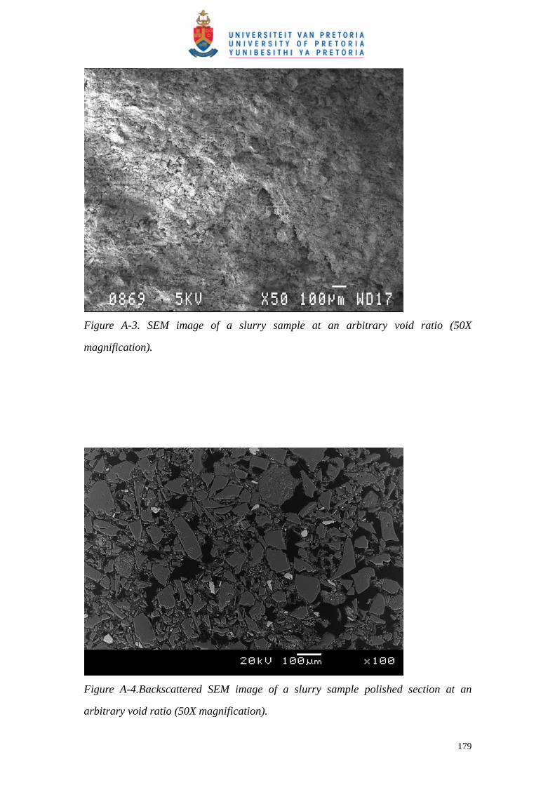
SEM images of various gold tailings samples were taken as a preliminary
investigation on the observable fabric and the possibilities with regards to using SEM
images. These include SEM images of moist tamped, slurry and in situ gold tailings
samples. Backscattered SEM images were also taken of the same samples prepared in
a polished section. Images obtained from the SEM are three-dimensional, while
Backscattered images are two-dimensional. The use of 2D (backscattered SEM) or 3D
(conventional SEM) images will thus need to be decided and evaluated from these
preliminary images.

178
Figure A-1. SEM image of a moist tamped sample at an arbitrary void ratio (50X
magnification).
Figure A-2. Backscattered SEM image of a moist tamped sample polished section at
an arbitrary void ratio (50X magnification).
179
Figure A-3. SEM image of a slurry sample at an arbitrary void ratio (50X
magnification).
Figure A-4.Backscattered SEM image of a slurry sample polished section at an
arbitrary void ratio (50X magnification).

180
Figure A-5. SEM image of in situ gold tailings (270X magnification).
Figure A-6. Environmental SEM image of moist tamped sample (300X magnification).

181
Appendix B
Instrumentation and Calibration
The calibration methodology used in this thesis has been described in Chapter 3.
Appendix B includes the specifications for the instrumentation used, the calibration
devices as well as the calibration, error and hysteresis graphs for all instrumentation.
An additional armature position test was also included for both LVDTs to investigate
the linear range of the apparatus.

182
Internal LVDT 1 Calibrated Instrument RDP 6385 D5/200WRA submissible LVDT/RDP
Transducer Amplifier Type S7AC Department Civil engineering, University of Pretoria Instrument no. 6385 Calibration device 1 YGP Tungsten Carbide Gauge Blocks Department National Metrology, CSIR Instrument no. 80112 Certificate no. DM/1177 Accuracy ±30 nm @ 20°C Calibration device 2 Mitutoyo ID-F150 Micrometer Department Civil Engineering, University of Pretoria Instrument no. 6049 Accuracy ±1.5 μm Data acquisition card National Instruments PCI-6014 Department Civil Engineering, University of Pretoria Instrument no. 1044CB9 Certificate no. 70772 Resolution 65536 bit Absolute accuracy 1 day 0.0154 % of reading 90 days 0.0174 % of reading 1 year 0.0196 % of reading DAQ card settings Sensor range -10V to +10V Input method Differential Channel 0
183
-8
-4
0
4
8
-15 -10 -5 0 5 10
Applied displacement (mm)
Out
put (
V)
(zero = 3)
(zero = 5)
(zero = 7)
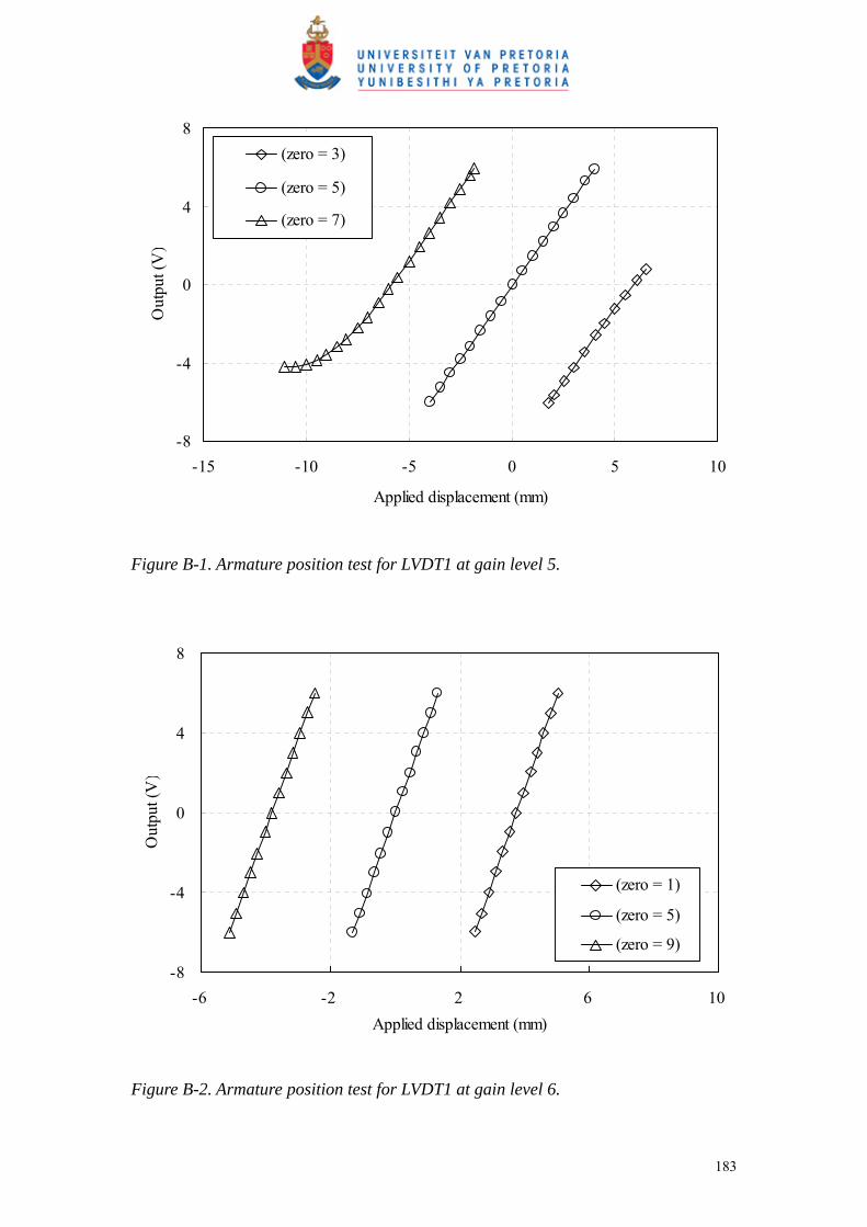
Figure B-1. Armature position test for LVDT1 at gain level 5.
-8
-4
0
4
8
-6 -2 2 6 10Applied displacement (mm)
Out
put (
V)
(zero = 1)
(zero = 5)
(zero = 9)
Figure B-2. Armature position test for LVDT1 at gain level 6.
184
-8
-4
0
4
8
-3 -1 1 3Applied displacement (mm)
Out
put (
V)
(zero = 1)
(zero = 5)
(zero = 9)
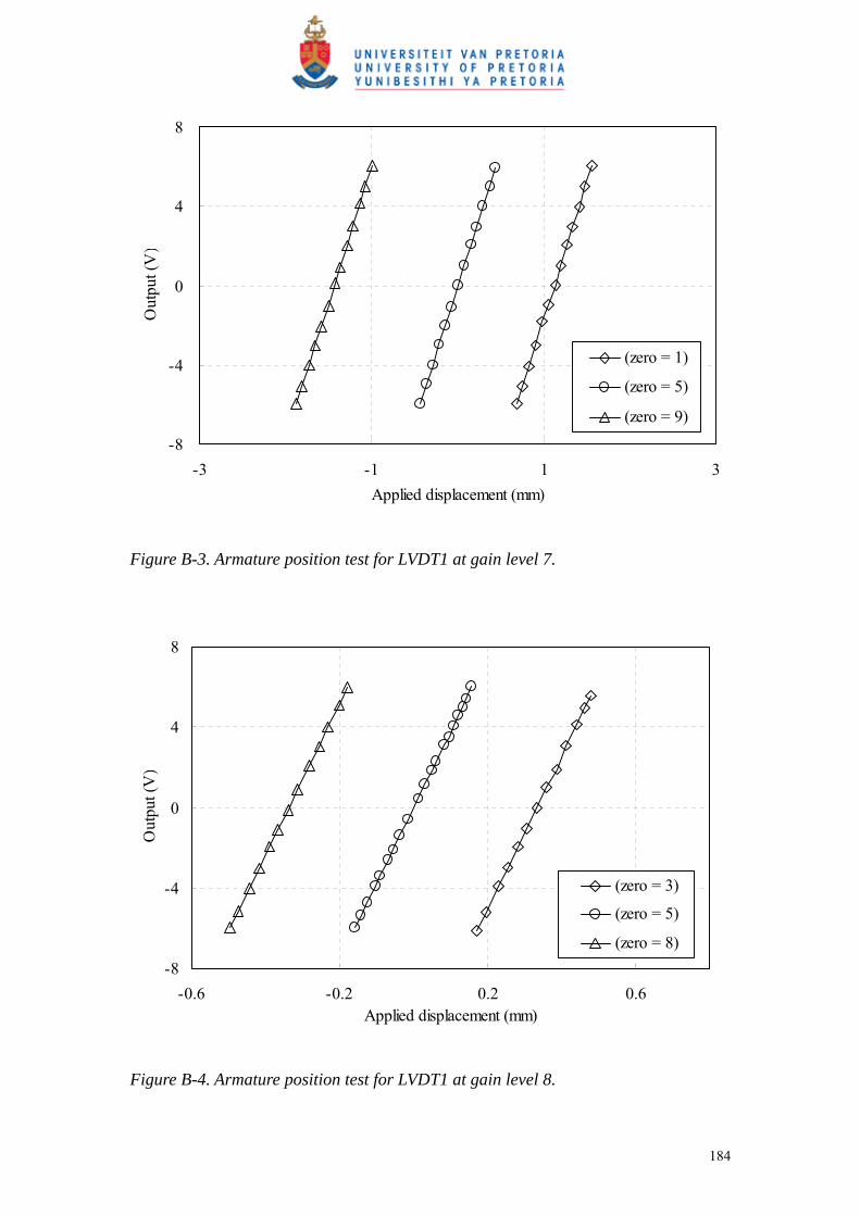
Figure B-3. Armature position test for LVDT1 at gain level 7.
-8
-4
0
4
8
-0.6 -0.2 0.2 0.6Applied displacement (mm)
Out
put (
V)
(zero = 3)
(zero = 5)
(zero = 8)
Figure B-4. Armature position test for LVDT1 at gain level 8.
185
-8
-4
0
4
8
-5 -4 -3 -2 -1 0 1 2 3 4 5Applied displacement (mm)
Out
put (
V)
Calibration (gain = 5)
Calibration (gain = 6)
Calibration (gain = 7)
Calibration (gain = 8)
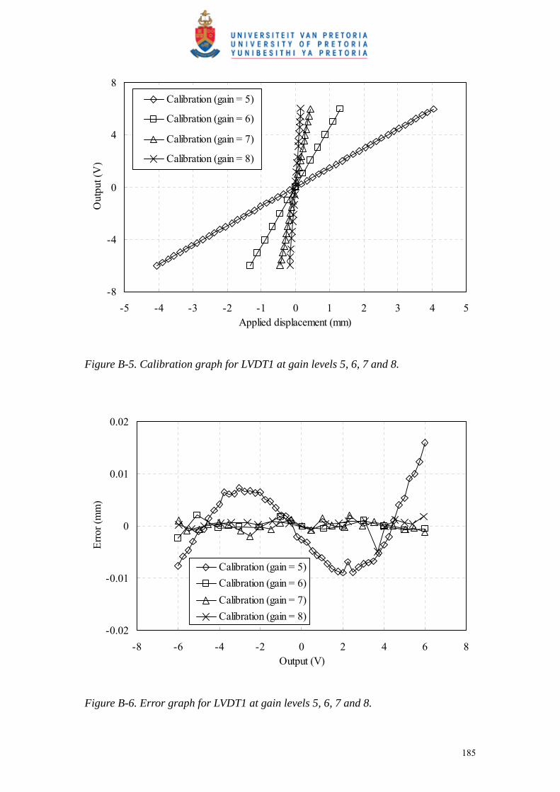
Figure B-5. Calibration graph for LVDT1 at gain levels 5, 6, 7 and 8.
-0.02
-0.01
0
0.01
0.02
-8 -6 -4 -2 0 2 4 6 8Output (V)
Erro
r (m
m)
Calibration (gain = 5)Calibration (gain = 6)Calibration (gain = 7)Calibration (gain = 8)
Figure B-6. Error graph for LVDT1 at gain levels 5, 6, 7 and 8.
186
-0.02
0
0.02
0.04
0.06
0.08
-6 -4 -2 0 2 4 6
Applied displacement (mm)
Out
put (
V)
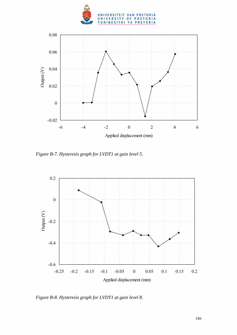
Figure B-7. Hysteresis graph for LVDT1 at gain level 5.
-0.6
-0.4
-0.2
0
0.2
-0.25 -0.2 -0.15 -0.1 -0.05 0 0.05 0.1 0.15 0.2
Applied displacement (mm)
Out
put (
V)
Figure B-8. Hysteresis graph for LVDT1 at gain level 8.

187
Internal LVDT 2 Calibrated Instrument RDP 6385 D5/200WRA submissible LVDT/RDP
Transducer Amplifier Type S7AC Department Civil engineering, University of Pretoria Instrument no. 6385 Calibration device 1 YGP Tungsten Carbide Gauge Blocks Department National Metrology, CSIR Instrument no. 80112 Certificate no. DM/1177 Accuracy ±30 nm @ 20°C Calibration device 2 Mitutoyo ID-F150 Micrometer Department Civil Engineering, University of Pretoria Instrument no. 6049 Accuracy ±1.5 μm Data acquisition card National Instruments PCI-6014 Department Civil Engineering, University of Pretoria Instrument no. 1044CB9 Certificate no. 70772 Resolution 65536 bit Absolute accuracy 1 day 0.0154 % of reading 90 days 0.0174 % of reading 1 year 0.0196 % of reading DAQ card settings Sensor range -10V to +10V Input method Differential Channel 1
188
-8
-4
0
4
8
-15 -10 -5 0 5 10Applied displacement (mm)
Out
put (
V)
(zero = 3)
(zero = 5)
(zero = 7)
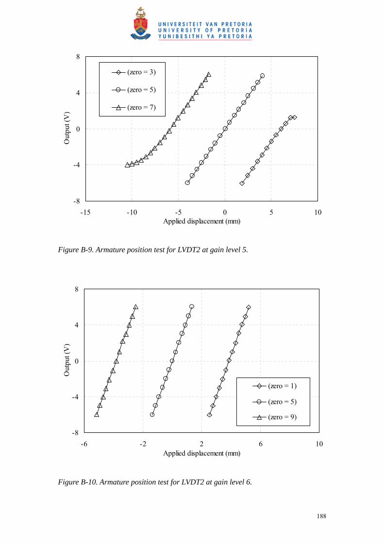
Figure B-9. Armature position test for LVDT2 at gain level 5.
-8
-4
0
4
8
-6 -2 2 6 10Applied displacement (mm)
Out
put (
V)
(zero = 1)
(zero = 5)
(zero = 9)
Figure B-10. Armature position test for LVDT2 at gain level 6.
189
-8
-4
0
4
8
-3 -1 1 3Applied displacement (mm)
Out
put (
V)
(zero = 1)
(zero = 5)
(zero = 9)
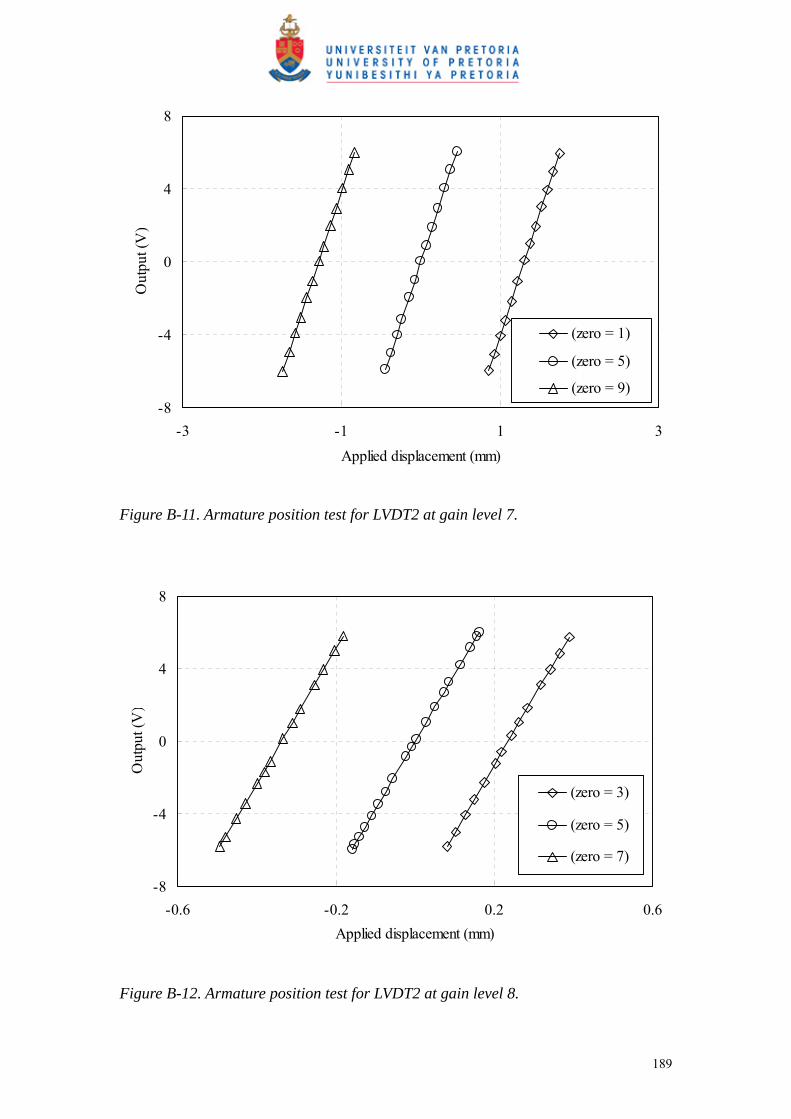
Figure B-11. Armature position test for LVDT2 at gain level 7.
-8
-4
0
4
8
-0.6 -0.2 0.2 0.6Applied displacement (mm)
Out
put (
V)
(zero = 3)
(zero = 5)
(zero = 7)
Figure B-12. Armature position test for LVDT2 at gain level 8.
190
-8
-4
0
4
8
-6 -4 -2 0 2 4 6Applied displacement (mm)
Out
put (
V)
Calibration (gain = 5)
Calibration (gain = 6)
Calibration (gain = 7)
Calibration (gain = 8)
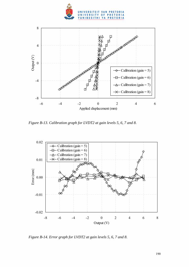
Figure B-13. Calibration graph for LVDT2 at gain levels 5, 6, 7 and 8.
-0.02
-0.01
0.00
0.01
0.02
-8 -6 -4 -2 0 2 4 6 8Output (V)
Erro
r (m
m)
Calibration (gain = 5)Calibration (gain = 6)Calibration (gain = 7)Calibration (gain = 8)
Figure B-14. Error graph for LVDT2 at gain levels 5, 6, 7 and 8.
191
-0.02
0
0.02
0.04
0.06
-6 -4 -2 0 2 4 6
Applied displacement (mm)
Out
put (
V)
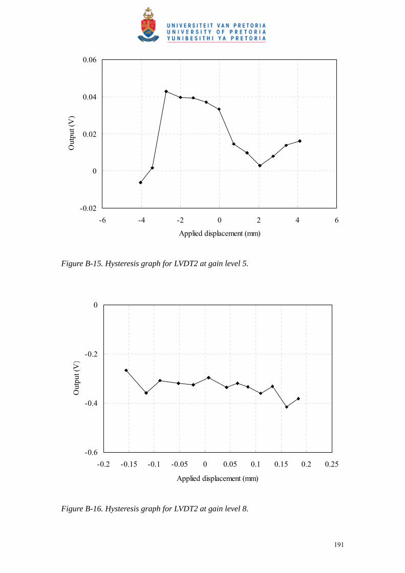
Figure B-15. Hysteresis graph for LVDT2 at gain level 5.
-0.6
-0.4
-0.2
0
-0.2 -0.15 -0.1 -0.05 0 0.05 0.1 0.15 0.2 0.25
Applied displacement (mm)
Out
put (
V)
Figure B-16. Hysteresis graph for LVDT2 at gain level 8.
192
Linear displacement transducer Calibrated Instrument Kyowa linear displacement transducer Department Civil engineering, University of Pretoria Instrument no. DT-20-D Serial no. YB-6279 Calibration device 1 YGP Tungsten Carbide Gauge Blocks Department National Metrology, CSIR Instrument no. 80112 Certificate no. DM/1177 Accuracy ±30 nm @ 20°C Calibration device 2 Mitutoyo ID-F150 Micrometer Department Civil Engineering, University of Pretoria Instrument no. 6049 Accuracy ±1.5 μm Data acquisition card National Instruments PCI-6014 Department Civil Engineering, University of Pretoria Instrument no. 1044CB9 Certificate no. 70772 Resolution 65536 bit Absolute accuracy 1 day 0.0154 % of reading 90 days 0.0174 % of reading 1 year 0.0196 % of reading DAQ card settings Sensor range -10V to +10V Input method Differential Channel 2 Amplifier HBM KWS 3073 Kal. Signal @ 2mV/V 4983 Measurements @ 1mV/V Channel 1
193
0
4
8
12
0 5 10 15 20 25
Applied displacement (mm)
Out
put (
V)
Gauge blocks
Micrometer
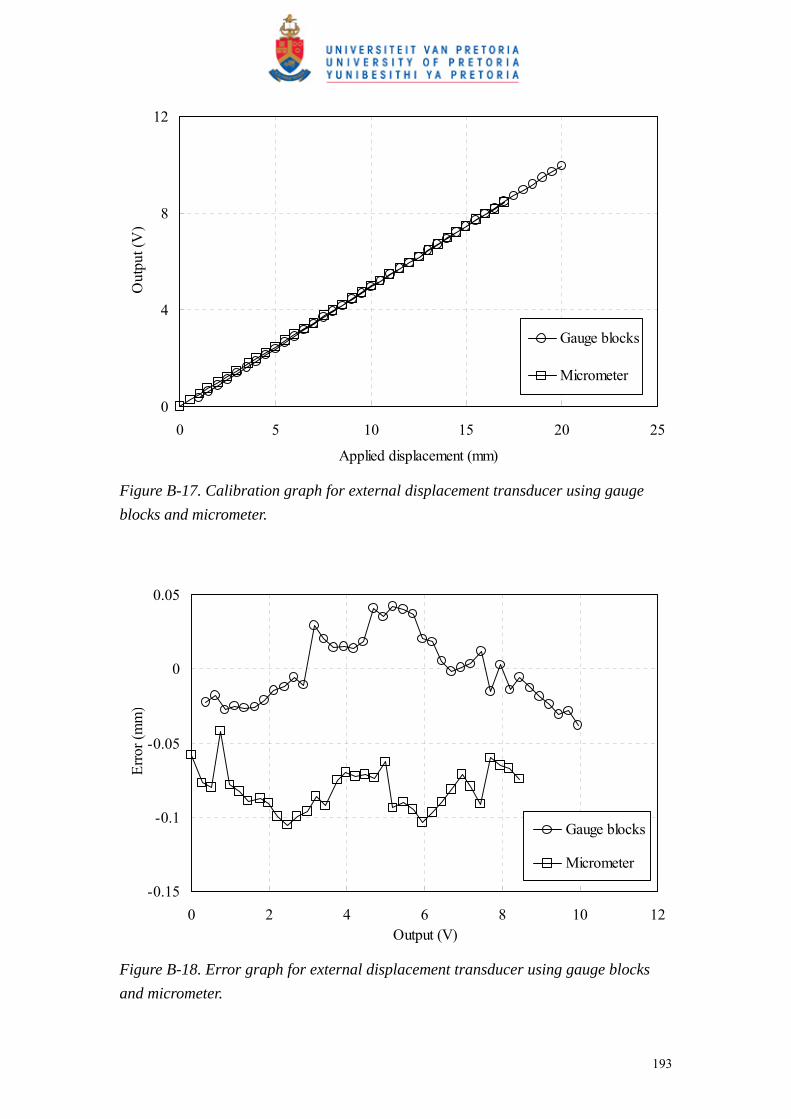
Figure B-17. Calibration graph for external displacement transducer using gauge blocks and micrometer.
-0.15
-0.1
-0.05
0
0.05
0 2 4 6 8 10 12Output (V)
Erro
r (m
m)
Gauge blocks
Micrometer
Figure B-18. Error graph for external displacement transducer using gauge blocks and micrometer.
194
-0.1
0
0.1
0.2
0.3
-5 0 5 10 15 20Applied displacement (mm)
Out
put (
V)
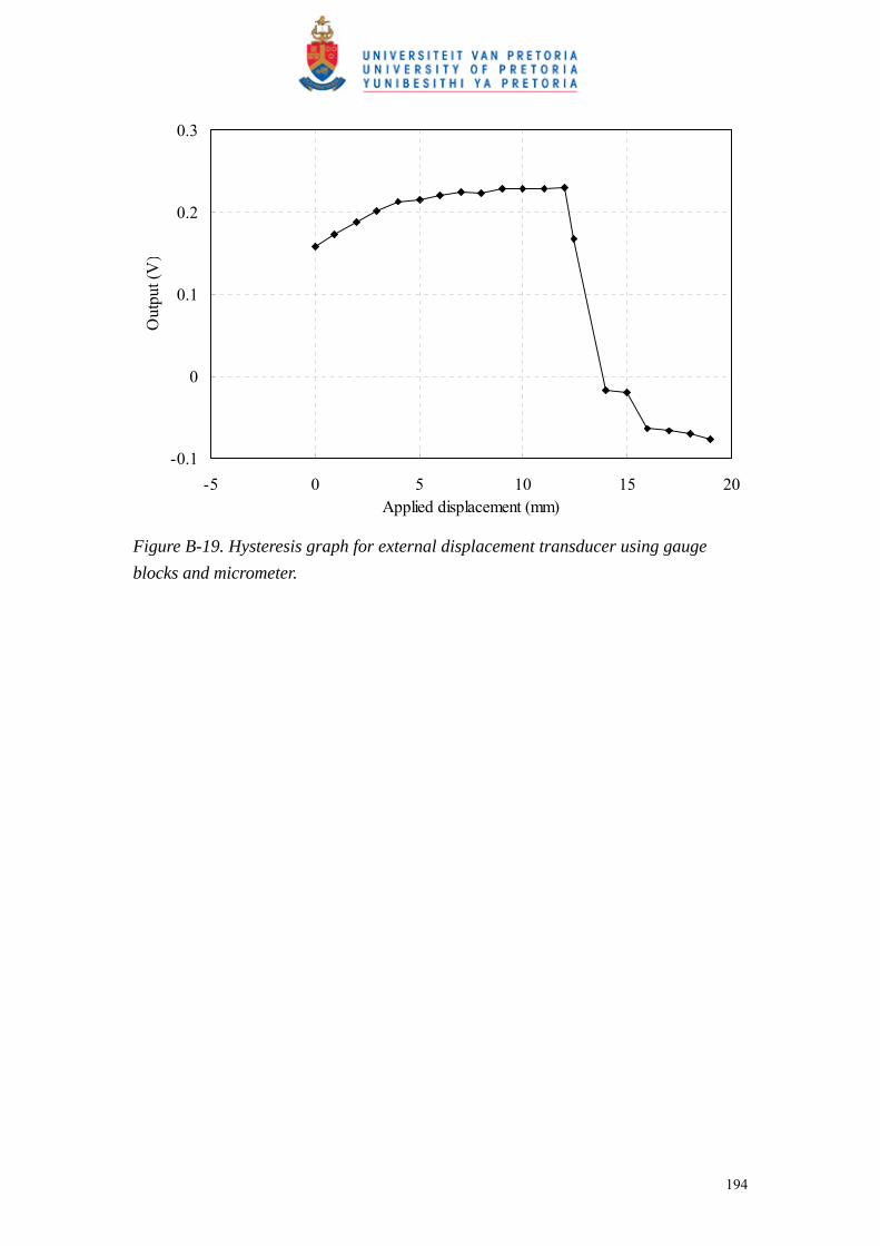
Figure B-19. Hysteresis graph for external displacement transducer using gauge blocks and micrometer.
195
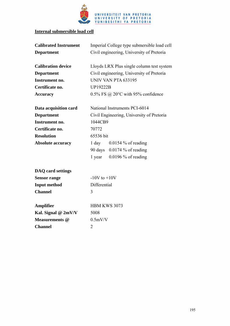
Internal submersible load cell Calibrated Instrument Imperial College type submersible load cell Department Civil engineering, University of Pretoria Calibration device Lloyds LRX Plus single column test system Department Civil engineering, University of Pretoria Instrument no. UNIV VAN PTA 633195 Certificate no. UP19222B Accuracy 0.5% FS @ 20°C with 95% confidence
Data acquisition card National Instruments PCI-6014 Department Civil Engineering, University of Pretoria Instrument no. 1044CB9 Certificate no. 70772 Resolution 65536 bit Absolute accuracy 1 day 0.0154 % of reading 90 days 0.0174 % of reading 1 year 0.0196 % of reading DAQ card settings Sensor range -10V to +10V Input method Differential Channel 3 Amplifier HBM KWS 3073 Kal. Signal @ 2mV/V 5008 Measurements @ 0.5mV/V Channel 2
196
0
2
4
6
8
10
0 200 400 600 800 1000 1200Applied force (N)
Out
put (
V)
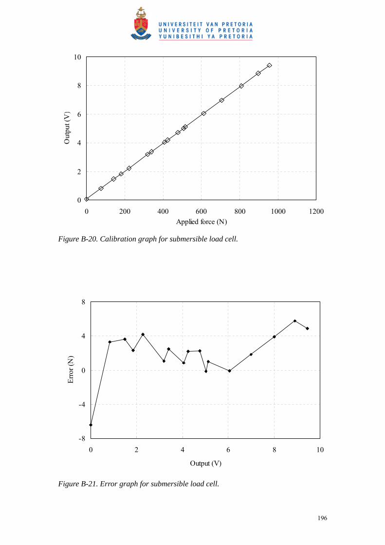
Figure B-20. Calibration graph for submersible load cell.
-8
-4
0
4
8
0 2 4 6 8 10
Output (V)
Erro
r (N
)
Figure B-21. Error graph for submersible load cell.
197
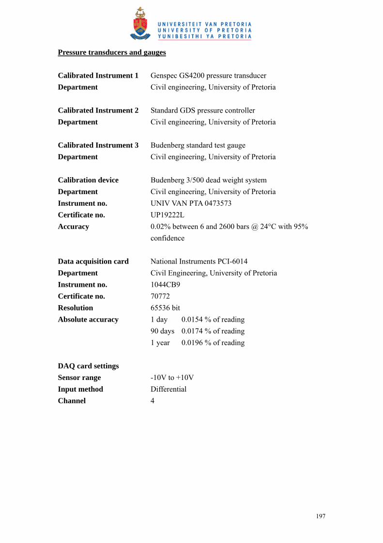
Pressure transducers and gauges Calibrated Instrument 1 Genspec GS4200 pressure transducer Department Civil engineering, University of Pretoria Calibrated Instrument 2 Standard GDS pressure controller Department Civil engineering, University of Pretoria Calibrated Instrument 3 Budenberg standard test gauge Department Civil engineering, University of Pretoria Calibration device Budenberg 3/500 dead weight system Department Civil engineering, University of Pretoria Instrument no. UNIV VAN PTA 0473573 Certificate no. UP19222L Accuracy 0.02% between 6 and 2600 bars @ 24°C with 95%
confidence
Data acquisition card National Instruments PCI-6014 Department Civil Engineering, University of Pretoria Instrument no. 1044CB9 Certificate no. 70772 Resolution 65536 bit Absolute accuracy 1 day 0.0154 % of reading 90 days 0.0174 % of reading 1 year 0.0196 % of reading DAQ card settings Sensor range -10V to +10V Input method Differential Channel 4

198
0
0.4
0.8
1.2
0 200 400 600 800 1000 1200
Applied pressure (kPa)
Out
put (
V)
Figure B-22. Calibration graph for pressure transducer.
0
2
4
6
8
10
0 200 400 600 800 1000 1200Applied pressure (kPa)
Out
put (
V)
0
200
400
600
800
1000
1200
Dig
ital p
ress
ure
cont
rolle
r (kP
a
Pressure transducer
Digital pressure controller
Budenberg test pressure gauge
Figure B-23. Calibration graph for pressure transducer, digital pressure controller and Budenberg test pressure gauge.
199
-6
-4
-2
0
2
4
0 200 400 600 800 1000 1200Applied pressure (kPa)
Erro
r (kP
a)
Pressure transducer
Digital pressure controller
Budenberg test pressure gauge
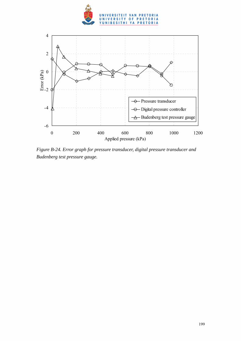
Figure B-24. Error graph for pressure transducer, digital pressure transducer and Budenberg test pressure gauge.

200
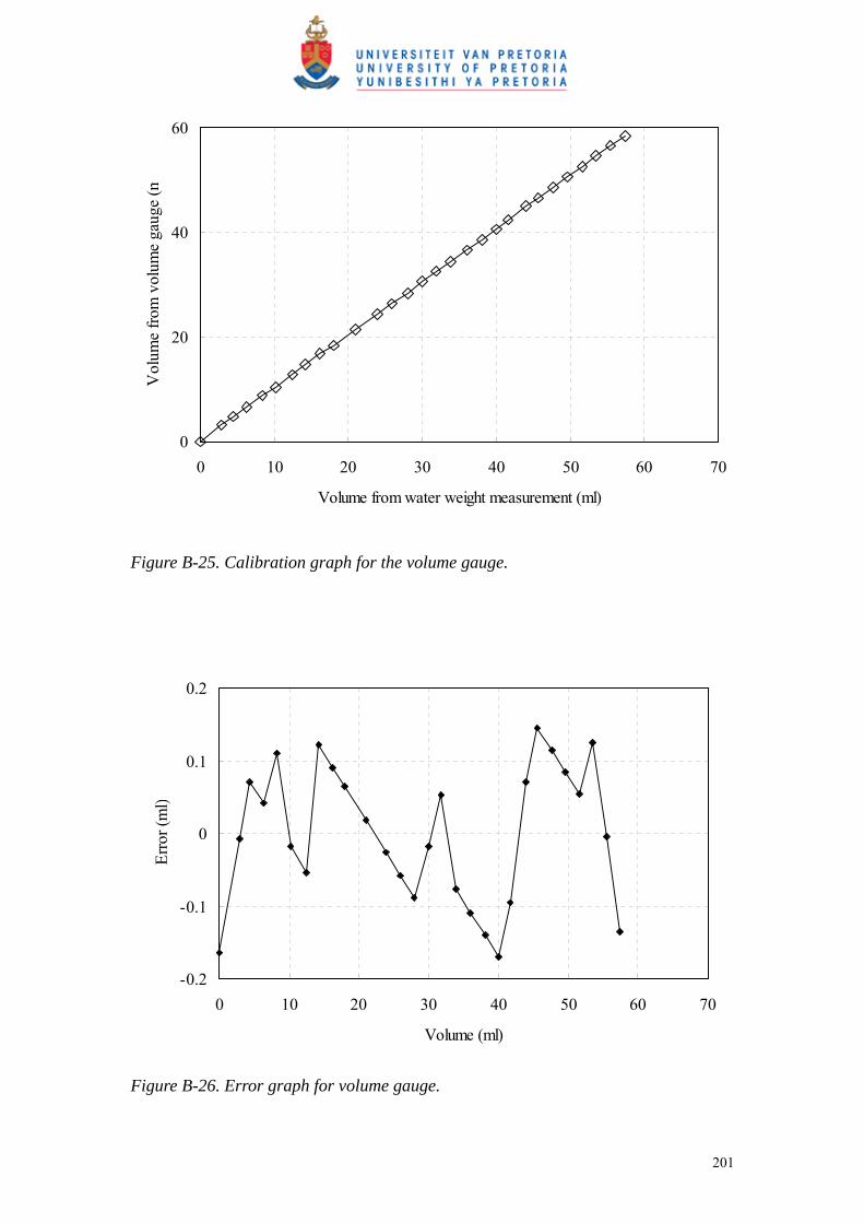
Volume gauge Calibrated Instrument Wykeham Ferrance volume gauge Department Civil engineering, University of Pretoria Calibration method Weight of water expelled at 21 °C Density of water 0.997968 Mg/m³ Resolution 0.1g
201
0
20
40
60
0 10 20 30 40 50 60 70
Volume from water weight measurement (ml)
Vol
ume
from
vol
ume
gaug
e (m
Figure B-25. Calibration graph for the volume gauge.
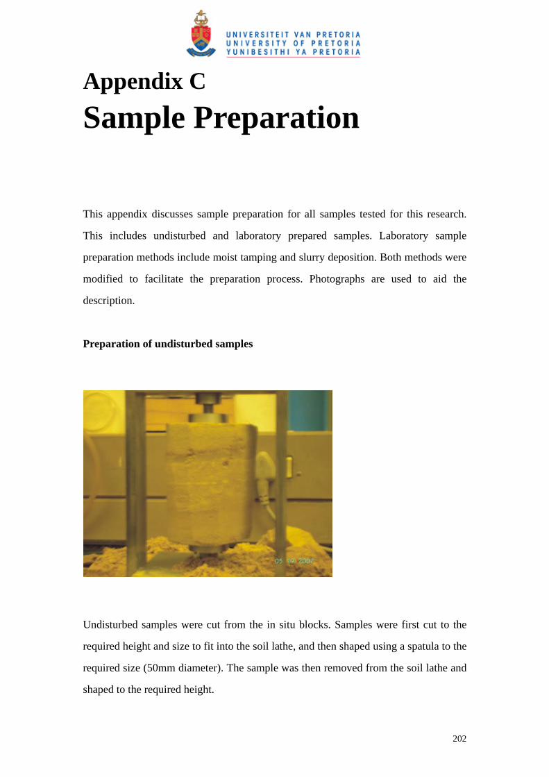
-0.2
-0.1
0
0.1
0.2
0 10 20 30 40 50 60 70
Volume (ml)
Erro
r (m
l)
Figure B-26. Error graph for volume gauge.
202
Appendix C Sample Preparation
This appendix discusses sample preparation for all samples tested for this research.
This includes undisturbed and laboratory prepared samples. Laboratory sample
preparation methods include moist tamping and slurry deposition. Both methods were
modified to facilitate the preparation process. Photographs are used to aid the
description.
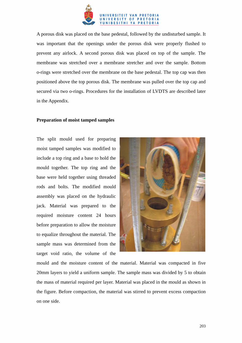
Preparation of undisturbed samples
Undisturbed samples were cut from the in situ blocks. Samples were first cut to the
required height and size to fit into the soil lathe, and then shaped using a spatula to the
required size (50mm diameter). The sample was then removed from the soil lathe and
shaped to the required height.
203
A porous disk was placed on the base pedestal, followed by the undisturbed sample. It
was important that the openings under the porous disk were properly flushed to
prevent any airlock. A second porous disk was placed on top of the sample. The
membrane was stretched over a membrane stretcher and over the sample. Bottom
o-rings were stretched over the membrane on the base pedestal. The top cap was then
positioned above the top porous disk. The membrane was pulled over the top cap and
secured via two o-rings. Procedures for the installation of LVDTS are described later
in the Appendix.
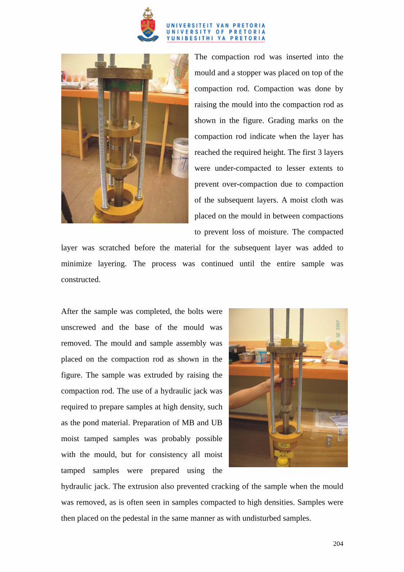
Preparation of moist tamped samples
The split mould used for preparing
moist tamped samples was modified to
include a top ring and a base to hold the
mould together. The top ring and the
base were held together using threaded
rods and bolts. The modified mould
assembly was placed on the hydraulic
jack. Material was prepared to the
required moisture content 24 hours
before preparation to allow the moisture
to equalize throughout the material. The
sample mass was determined from the
target void ratio, the volume of the
mould and the moisture content of the material. Material was compacted in five
20mm layers to yield a uniform sample. The sample mass was divided by 5 to obtain
the mass of material required per layer. Material was placed in the mould as shown in
the figure. Before compaction, the material was stirred to prevent excess compaction
on one side.
204
The compaction rod was inserted into the
mould and a stopper was placed on top of the
compaction rod. Compaction was done by
raising the mould into the compaction rod as
shown in the figure. Grading marks on the
compaction rod indicate when the layer has
reached the required height. The first 3 layers
were under-compacted to lesser extents to
prevent over-compaction due to compaction
of the subsequent layers. A moist cloth was
placed on the mould in between compactions
to prevent loss of moisture. The compacted
layer was scratched before the material for the subsequent layer was added to
minimize layering. The process was continued until the entire sample was
constructed.
After the sample was completed, the bolts were
unscrewed and the base of the mould was
removed. The mould and sample assembly was
placed on the compaction rod as shown in the
figure. The sample was extruded by raising the
compaction rod. The use of a hydraulic jack was
required to prepare samples at high density, such
as the pond material. Preparation of MB and UB
moist tamped samples was probably possible
with the mould, but for consistency all moist
tamped samples were prepared using the
hydraulic jack. The extrusion also prevented cracking of the sample when the mould
was removed, as is often seen in samples compacted to high densities. Samples were
then placed on the pedestal in the same manner as with undisturbed samples.
205
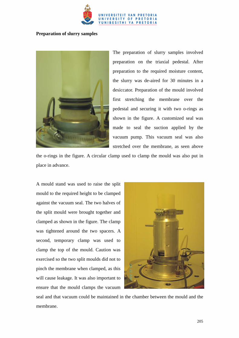
Preparation of slurry samples
The preparation of slurry samples involved
preparation on the triaxial pedestal. After
preparation to the required moisture content,
the slurry was de-aired for 30 minutes in a
desiccator. Preparation of the mould involved
first stretching the membrane over the
pedestal and securing it with two o-rings as
shown in the figure. A customized seal was
made to seal the suction applied by the
vacuum pump. This vacuum seal was also
stretched over the membrane, as seen above
the o-rings in the figure. A circular clamp used to clamp the mould was also put in
place in advance.
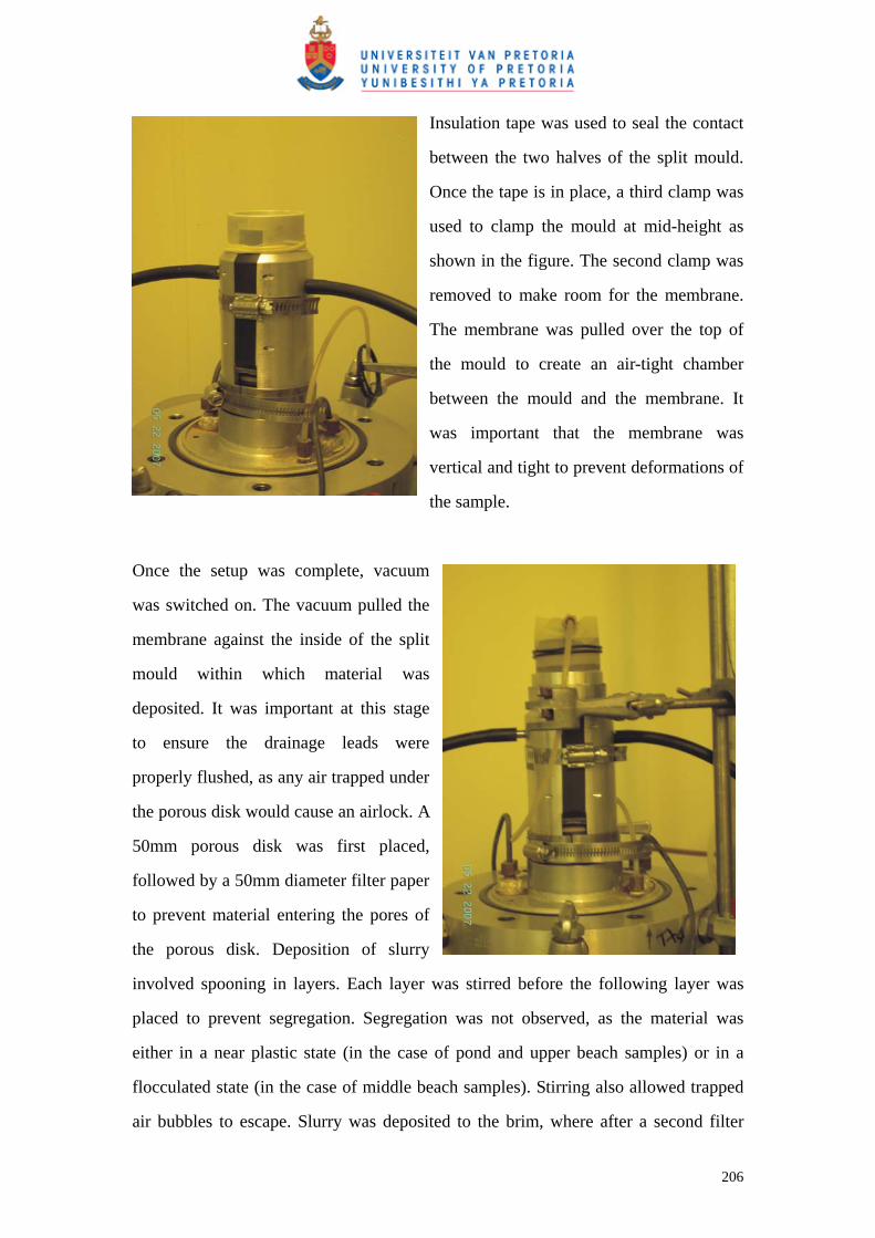
A mould stand was used to raise the split
mould to the required height to be clamped
against the vacuum seal. The two halves of
the split mould were brought together and
clamped as shown in the figure. The clamp
was tightened around the two spacers. A
second, temporary clamp was used to
clamp the top of the mould. Caution was
exercised so the two split moulds did not to
pinch the membrane when clamped, as this
will cause leakage. It was also important to
ensure that the mould clamps the vacuum
seal and that vacuum could be maintained in the chamber between the mould and the
membrane.
206
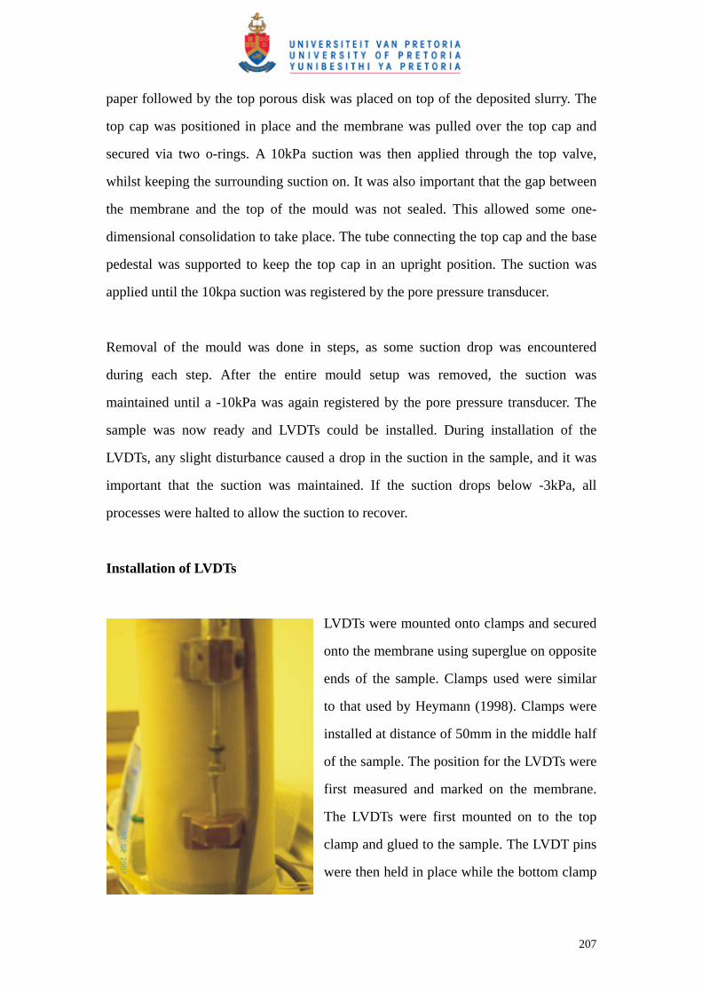
Insulation tape was used to seal the contact
between the two halves of the split mould.
Once the tape is in place, a third clamp was
used to clamp the mould at mid-height as
shown in the figure. The second clamp was
removed to make room for the membrane.
The membrane was pulled over the top of
the mould to create an air-tight chamber
between the mould and the membrane. It
was important that the membrane was
vertical and tight to prevent deformations of
the sample.
Once the setup was complete, vacuum
was switched on. The vacuum pulled the
membrane against the inside of the split
mould within which material was
deposited. It was important at this stage
to ensure the drainage leads were
properly flushed, as any air trapped under
the porous disk would cause an airlock. A
50mm porous disk was first placed,
followed by a 50mm diameter filter paper
to prevent material entering the pores of
the porous disk. Deposition of slurry
involved spooning in layers. Each layer was stirred before the following layer was
placed to prevent segregation. Segregation was not observed, as the material was
either in a near plastic state (in the case of pond and upper beach samples) or in a
flocculated state (in the case of middle beach samples). Stirring also allowed trapped
air bubbles to escape. Slurry was deposited to the brim, where after a second filter
207
paper followed by the top porous disk was placed on top of the deposited slurry. The
top cap was positioned in place and the membrane was pulled over the top cap and
secured via two o-rings. A 10kPa suction was then applied through the top valve,
whilst keeping the surrounding suction on. It was also important that the gap between
the membrane and the top of the mould was not sealed. This allowed some one-
dimensional consolidation to take place. The tube connecting the top cap and the base
pedestal was supported to keep the top cap in an upright position. The suction was
applied until the 10kpa suction was registered by the pore pressure transducer.
Removal of the mould was done in steps, as some suction drop was encountered
during each step. After the entire mould setup was removed, the suction was
maintained until a -10kPa was again registered by the pore pressure transducer. The
sample was now ready and LVDTs could be installed. During installation of the
LVDTs, any slight disturbance caused a drop in the suction in the sample, and it was
important that the suction was maintained. If the suction drops below -3kPa, all
processes were halted to allow the suction to recover.
Installation of LVDTs
LVDTs were mounted onto clamps and secured
onto the membrane using superglue on opposite
ends of the sample. Clamps used were similar
to that used by Heymann (1998). Clamps were
installed at distance of 50mm in the middle half
of the sample. The position for the LVDTs were
first measured and marked on the membrane.
The LVDTs were first mounted on to the top
clamp and glued to the sample. The LVDT pins
were then held in place while the bottom clamp

208
was glued in place. The pins rested on a flat-headed screw in the bottom clamp. The
screws could be used to adjust the initial position of the armature and therefore the
initial output of the LVDTs. This was required to accommodate for volume changes
before shear so that shearing could start in the range of the highest gain (8).
Installation of LVDTs was done in this manner for all samples tested.