~"''; .. ',

~,,)

," u. iii

STATUS OF THE

Bay Protectionand

Toxic CleanupProgram

Appendices

State Water Resources Control BoardRegional Water Quality Control Boards

STATE OF CALIFORNIAPete Wilson, Governor

CALIFORNIA ENVIRONMENTAL PROTECTION AGENCYJames M. Strock, Secretary

STATE WATER RESOURCESCONTROL BOARDP.O. Box 100Sacramento, CA 95812~0100

(916) 657·2390

John Caffrey, MemberMarc Del Piero, MemberJames M. Stubchaer, Member

Walt Pettit, Executive DirectorDale Claypoole, Deputy Director

•

1

STATUS Of TillIE'BAVIPROTECHOOO Mil TOXIC ClEA~UIP IPIROGIWW

STAfFREPC:RT

APPIENDICIES

STATE ~ATER RESOURCES CO~lROl BOARD

STATE OF CAlIfOROOXA

APPENDIX A:

APPENDIX B:

APPENDIX C:

APPENDIX 0:

APPENDIX E:

APPENDIX F:

LIST Of APPE~DICES

Bay Protection and Toxic Cleanup Program Water Code Sections(Chapter 5.6, Sections 13390 et seq. of the Water Code)

List of Reports Prepared Fully or in Part by the BPTCP(including Contractor Reports)

San Francisco Bay Pilot Regional Monitoring Program 1991-1992Summary Progress Report

Strategy for Establishing Sediment Quality Objectives based onHuman Health Risk Assessment

Staff Report: Criteria to Rank Toxic Hot Spots in EnclosedBays and Estuaries of California

Senate Bill 1084 (Calderon) (Statutes 1993, Chapter 1157)

A P P [ ~ D I X A

Bay Protectio~ and Toxic tlea~Mp ProgramWater Code Sections

Chapter 5.6 of the Water CodeSections 13390 et seq.

..

by the defendant personally, cannot be attributed to thedefendant.

(e) Any person who knowingly makes any false statement,representation, or certification in any record, report, plan, orother document filed with a regional board or the state board,or who knowingly falsifies, tampers with, or rendersinaCCurate any monitoring device or method required underthis division shall be punished by a fine of not more thantwenty-five thousand dollars ($ 25,000), or by imprisonmentfor not more than two years, or by both. If a conviction of aperson is for a violation committed after. a first conviction ofthe person under this subdivision, punishment shall be by afine of not more than twenty-five thousand dollars ($ 25,000)per day of violation, or by imprisonment of not more thanfour years, or by both.

(t) For purposes of this section, a single operational upsetwhich leads to simultaneous violations of more than onepollutant parameter shall be treated as a single violation.

(g) For purposes of this section, "organization." "seriousbodily injury," "person,' and " hazardous substance" shallhave the same meaning as in Section 309(c) of the FederalWater Pollution Control Act, as amended.

(h) Funds collected pursuant to this section shall be paid tothe State Water Pollution Cleanup and Abatement Account.

HISTORY: Added SUIIS 1987 en 1189 § 14.[Fonner Section: Fomur § 13387, simil4r 10 the present section,Added SlOts 1972 en 1256 § 1, effective December 19, 1972:Amended SlOts 1978 en 746 § ll: S,ats 1984 en 1541 § 8:Repealed Slats 1987 en 1189 § lJ.}

§ 13388. Board member eligibility

Notwithstanding any other provision of this division or Section175, no person shall be a member of the state board or aregional board if he receives or has received during theprevious two years a significant portion of his income directlyor indirectly from any person subject to waste dischargerequirements or applicants for waste discharge requirementspursuant to this chapter. This section shall become operativeon March 1. 1973.

HISTORY: Added S,ats 1972 en 1256 § 1, effective December 12,1972.

§ 13389. Exemption of bo~rds from certain provisions ofthe California Environmental Quality Act

Neither the state board nor the regional boards shall berequired to comply with the provisions of Chapter 3(commencing with Section 21100) of Division 13 of the PublicResources Code prior to the adoption of any waste discharge

_-.. •• ~ · .... r ..( _

~. except requirements fOll' new aoorc:es llS aMedin the Federal WsWI' Pollution Control Act or acts ammdatorythereof or supplementary thereto.

HIsToRY: M:!l4tl S-1971ck 1236 ft 1, 'iflqedw.~12,1Jm.

~ 5.'. .y ffiroaetlliODD md 'l!'ome CleanUJlll

§ n33~. Intent

It is the intent of the Legislature that the state board and theregional 00ards establish programs that provide mWmumprotection for existing mllCl future beneI1icial uses of boy llIldestuarine wnters. llIld tbat abese progmms include a plan forremedisl eeUoo at tolXie ho¢ spots. It is oIso the intent of theLegislature that theea programs further compliance withfederal Jaw pertaining to the identification ofwaters where theprotection nod propagntioo of shellfish, fish, and wild1ife arethreatened by toltic pollutants mtd contribute to thedevelopment of effective strategies to control these pollutants.It is also the intent of the Legislature that these progrnms bestructured ODd maintained in a IDlIIIIteI' which allows the stateboard and the regioaal boords to IDll!ce Jm!ximum use of anyfederal f'ueds which may be available for any of the purposesspecified in this chapter.

HISTORY: AiltIed StDU 1989, d1269. § JO, e.ff«tm August J. 1989.

§ 13391. Formulation, adoption and implementation ofCalifornia &closed Bays and Estuaries Plan

(a) The state board shaD formulate and adopt a water qualitycontrol plan for enclosed bays nd estuaries, which shall belcnown as the California Enclosed Bays and Estuaries PIan, inaccordance with the procedures established by this division foradopting water quality control plans.

(b) As part of its formulation and adoption of the CaliforniaEnclosed Bays and Estuaries Plan, the state board shall reviewand update the Water Quality Control Policy for EnclosedBays and Estuaries of California, as adopted in 1974 puJSUaDtto Article 3 (commencing with Section 13140) of Chapter 3;and incorporate the results of that review and update in theCalifornia Enclosed Bays and Estuaries Plan.

(c) State and regional offices, departments, boards andagencies shall fully implement the California Enclosed Baysand Estuaries Plan. Pending adoption of the CaliforniaEnclosed Bays and Estuaries Plan by the state board, state andregional offices, departments, boards and agencies shall fullyimplement the Water Quality CootroCPolicy- Jar EnclosedBays and Estuaries of California. - - - ..

(d) Each regional board shall review tlDd, ifnecessary. revise

CHAPl'ER 5.6. Bay Protection and Toxic Cleanup

waste discharge requirements that are inconsistent with thosepolicies and principles.

HISTORY: Added Stall 1989 ch 269 § SO. elfecdwt AuglUtJ. J989; AmendedStall 1989 cit 1032. t 30. <!fectlve &ptember 29. 1989.

§ 13391.5. Definitions

The definitions in this section govern the construction of thischapter.

(a) wEnclosed baysw means indentations along the coast whichenclose an area of oceanic water within distinct headlands orharbor works. wEnclosed baysw include all bays where thenarrowest distance between the headlands or outermost harborworks is less than 75 percent of the greatest dimension of theenclosed portion of the bay. wEnclosed bays" include, but arenot limited to, Humboldt Bay, Bodega Harbor, Tomales Bay, _Drake's Estero, San Francisco Bay, Morro Bay, Los Angeles-­Long Beach Harbor, Upper and Lower Newport Bay, MissionBay, and San Diego Bay. For the purposes of identifying,characterizing, and ranking toxic hot spots pursuant to thischapter, Monterey Bay and Santa Monica Bay shall also beconsidered to be enclosed bays.

(b) "EstuariesW means waters, including coastal lagoons,located at the mouths of streams which serve as mixing zonesfor fresh and ocean waters. Coastal lagoons and mouths ofstreams which are temporarily separated from the ocean bysandbars shall be considered as estuaries. Estuarine watersshall be considered to extend from a bay or the open ocean toa point upstream where there is no significant mixing of freshwater and sea water. Estuarine waters include, but are notlimited to, the Sacramento-San Joaquin Delta, as defined inSection 12220, Suisun Bay, Carquinez Strait downstream tothe Carquinez Bridge, and appropriate areas of the Smith.Mad, Eel, Noyo, Russian, Klamath, San Diego, and OtayRivers.

(c) wHealth risk assessmentW means an analysis whichevaluates and quantifies the potential human exposure to apollutant that bioaccumulates or may bioaccumulate in ediblefish, shellfish, or wildlife. "Health risk assessment" includesan analysis of both individual and population wide health risks ­associated with anticipated levels of buman exposure.including potential synergistic effects of toxic pollutants andimpacts on sensitive populations.

(d) "Sediment quality objective" means that level of aconstituent in sediment which is established with an adequatemargin of safety, for the reasonable protection of mebeneficial uses of water or the prevention of nuisances.

(e)WToxic hot spotsWmeans locations in enclosed bays,

Po~ColDBne Waur QuaUty Control..te, ami Relaud Codu • J992, - PAGE 44

.V .'~

estuaries, or any adjacent waters in the wcontiguoUS moeworthe Wocean, W as defined in SectiOD 502 of the Clean WaJer ki.(33 U.S.C. Sec. 1362), the pollution or contamination ofwhich affects the interests of the state, IIId where hazardoua'substances have accumuJattd in the water or sediment to leveJawhich (1) may poSe • substantial present or potential hazardto aquatic life, wildlife, fisheries, or human health, or (2) mayadversely affect the beneficial uses of the bay, estuary, orocean waters as defined in water quality toDtrol plans, or (3)exceeds adopted water quality or sediment qualjty objectives.

(f) wHazardous substancesw has the SlUIIe meaning IS definedin subdivision (f) of Section 25281 of the Health and SafetyCode.

HlS70RY: Added Stall 1989 ell 269 t SO, qfecrtn AU8. J, J989; AmentldStall J989ch JOn. 0 30. eJ!«dwS#pt. 29. lfJ1J9;SJaa 1991 cIr J09J 0162.

A 13392. Toxic hot spots program"','~

The state board and the regional boards, in consultation withthe Office of EnvironmeutaJ Health Hazard Assessment andthe Department of Fish and Game. sha1J develop and maintain• compre-hensive program to (1) identify and characterizetoxic hot spots, as defined in Section 13391.5, (2) plan for the ­~leanup or other appropriate remedial or mitigating actions atthe sites, and (3) amend water quality control plans andpolicies to incorporate strategies to prevent the creation of

- new toxic hot spots and the further pollution of existing hotspots. As part of this program. the state board and regionalboards shall, to the extent feasible, identify specific dischargesor waste management practices which contnDute to thecreation of toxic hot spots, and shall develop appropriateprevention strategies, including, but not limited to, adoptionof more stringent waste discharge requirements, onshoreremedial actions, adoption of regulations to control sourcepollutants, and development of new programs to reduce urban .,and agricultural ronoff.

HlS70RY: Added Stall 1989 cIr 269 t SO, dfecdw AUBIIl' 3. 1989;

Gowmor~ Reo"ClllhAdon Pfdn. No.1. 1991. 1191. ' I

§ 13392.5. Data base identifying and descn"bing-toxic hotspots; Monitoring and surveillance task force

(a) Each regional board which has regulatory authority (orone or more enclosed bays or estuaries shall. by January I,1992, develop for each enclosed bay or estuary, aconsolidated data base which identifies and describes aUknown and suspected toxic bot spots. Each regional boardshall, in consultation with the state bOald,-aIso develop anongoing monitoring and surveillance program that includes,but is not limited to, the fonowing components:

-I

..

,

caArtER 5.6. Bay JPTotediorm ancll1"o)j;ic Cleanup

(1) Establishment of l!l monitoring and surveillance task forcethat includes representation from agencies, including, butnot limited to, the Office of Environmental Health HazardAsseSSment and the Department of Fish and Game, thatroutinely monitor water quality, sediment, and aquatic

life.

(2) Suggested guidelines to promote standardized analyticalmethodologies and consistency in data reporting.

(3) Identification of additional monitoring and analyses thatare needed to develop a complete toxic bot spotassessment for each enclosed bay and estuary.

(b) Each regional board shall make available to state andlocal agencies and the public all information contained in theconsolidated data base, as well as the results of newJDOnitoring and surveillance data.

HlSTORY: Added SIDI3 1989 ch 269 § :SO, effecnye Augusl 2, 1989; AmendedSI4U 1989 ch 1032 § 32, effecnye Seplember 29, 1989; Goyernor'sReorganiZ/Jnon Plan, No.1, 1991, § 198.

§ 13392.6. Workplan for adoption of sediment qualitythresholds for toxic pollutants

(a) On or before July 1, 1991, the state board shall adopt andsubmit to the Legislature a workplan for the adoption ofsediment quality objectives for toxic pollutants that have beenidentified in known or suspected toxic hot spots and for toxicpollutants that have been identified by the state board or aregional board as a pollutant of concern. The workplan shallinclude priorities and a schedule for development and adoptionof sediment quality objectives, identification of additionalresource needs, and identification of staff or funding needs.The state board is not prohibited from adopting sedimentquality objectives in the workplan for a constituent for whichthe workplan identifies additional research needs.

(b) In preparing the workplan pursuant to subdivision (a), thestate board shall conduct public hearings and workshops andshall consult with persons associated with municipaldischarges, industrial discharges, other public agencies,research scientists, commercial and sport fishing interests,marine interests, organizations for the protection of naturalresources and the environment, and the general public.

HISTORY: Added SI4U 1989ch 269 § 50,effecdye AuglU12, 1989; AmendedSuus 1989 ch 1012 § 33, effeedye September 29,1989.

§ 13393. Sediment quality objectives

The state board shaH adopt sediment quality objectivespursuant to the workplan submitted pursuant to Section

13392.6. The state board shall adopt the sediment qualityobjectives pUfSUlllDt to the procedures established by thisdivision for adopting or M!f:Oding water quality control plans.The sediment quality objectives sball be based on scientificinformation, including, but not limited to, chemicalmonitoring, bioassays oresaablished modeling procedures, andshall provide adequate protection for the most sensitive aquaticorganisms. The state board shall base the sediment qualityobjectives on a health risk assessment if there is a potential forexposure of humans to poUutants through the food chain toedible fish, shellfish, or wildlife.

HISTORY: MUd SIDI:I 1989 cit Ion i 15, eJf«tive Septmtber 29, 1989.[Fonner Secdtm.· Fomer \\ JJJ9J, 6imU4r to lite prueJll,eclton,- tuUkd SIDI:I 19l19 ell 2691l SO, efficdw Au,..., 2, 1989, IIlUI"pealed S_ 1989dt Ion 1l34, e~CIlW! Sept. 29,1989].

§ 13393.5. A.sse.ssn=lt and priority ranking of toxic hot spots

On or before July 1, 1992, the state board, in consultationwith the Office of Environmental Health Hazard Assessmentand the Department of Fish and Game, shall adopt generalcriteria for the assessment and priority ranking of toxic hotspots. The criteria shall talce into account the pertinent factorsrelating to public health and environmental quality, including,but not limited to, potential hazards to public health, toxichazards to fish, shellfish, tmd wildlife, and the extent to whichthe deferral of a remedial action will result or is likely toresult in a significant increase in environmental damage,health risks, or cleanup costs.

HISTORY: Added SIDI:I 1989 cll 269, § :SO, e.ffet:dW! Aug. 3, 1989; AmmdedGovernor', ReorgfJltiuukm PlaIa. No.1, 1991, § 199.

§ 13394. Toxic bot spot cleanup plans

On or before July I, 1993, each regional board shall completeand submit to the state board a toxic hot spots cleanup plan.On or before January 1, 1994, the state board shall submit tothe Legislature a consolidated statewide toxic hot spotscleanup plan. The cleanup plan submitted by each regionalboard and the state board shall include, but not be limited to,the following informatian: '

(a) A priority ranlcing of all hot spots, including the stateboard's recommendations for remedial action at each toxic hotspot site.

(b) A description of each hot spot site including acharacterization of the pollutants presentat the site.

(c) An estimate of the total costs to impIe~-t theplan.

(d) An assessment of abe most likely source or sources of

CHAPI'ER 5.6. Bay Protedion and Toxic. Cleanup

pollutants.

(e) An estimate of the costs that may be reeovemble fromparties respoosible for the discharge of pollutants that haveaccumulated in sediment.

(f) A preliminary assessment of the actions required toremedy or restore a toxic hot spot.

(g) A two-year expenditure schedule identifying state fundsneeded to implement the plan.

(h) A summary of actioos that have been initiated by theregional board to reduce the accumulation of pollutants atexisting hot spots and to prevent the creation of new hot spots.

(i) The plan submitted by the state board shall includefindings and recommendations concerning the need for~tablishment of a toxic hot spots cleanup program.

HISTORY: Added S'aU 1989 ch 269. § SO. (ffecdve Aug. J, 1989.

§ 13394.5. Annual Expenditure Plan

The state board, as part of the annual budget process, shallprepare and submit to the Legislature a recommended annualexpenditure plan for the implementation of this chapter.

to revise a waste discharge requirement oo1y if it finds that thetoxic hot spot resulted from practices no longer beingconducted by the discharger or permitted under the existingwaste discharge requin:ment, or that the discharger'scontribution to the creation or maintenance of the toxic hotspotisnotsignificanL

HlSTORY: Add" Slau 1939 dJ 269 § 10. (ff«rlve August 2, 1989.

§ 13395.5. Contmcts and Other Agreements

The state board may enter into contracts and other agreementafor the purpose ofevaluating or demonstrating methods for theremoval, treatmePt, or stabilization of contaminated bottomsediment. For the purpose ofpreparing health risk assessments·pursuant to Section 13393, the state board shall enter intocontracts or agreements with the Office of Environmental

, Health Hazard Assessment, or with other state or localagencies, subject to the approval of the office. The costsincurred for worle conducted by other state agencies,including, but not limited to, the office and the Department ofFish and Game, pursuant to this chapter shall be reimbursedaccording to the tenIL'l of an interagency agreement betweenthe state board and the agency.

HlSTORY: Added S/.QU 1989, dt 269, I 10, ~eetlw! Augw' J, 1989;Governor's .Reorgan/vUiOll PIim, No.1, 1991, § 200.

"

,.,

r

H1STORY: Added S'au 1989 ch 269, § SO, (ffecdve Aug. J, 1989.

§ 13395, Reevaluation of waste discharge requirements fordischarge into toxic hot spots

Each regional board shall, within 120 days from the rankingof a toxic hot spot, initiate a reevaluation of waste dischargerequirements for dischargers who, based on the determinationof the regional board, have discharged all or part of thepollutants which have caused the toxic hot spot. Thesereevaluations shall be for the purpose of ensuring compliancewith water quality control plans and water quality control planamendments. These reevaluations shall be initiated accordingto the priority ranking established pursuant to subdivision (a)of Section 13394 and shall be scheduled so that, for eachregion, the first reevaluation shall be initiated within 120 daysfrom, and the last shall be initiated within one year from. theranking of the toxic hot);pot,s. The regional board shall,consistent with the policies ana principles set forth in Section13391, revise waste discharge requirements to ensurecompliance with water quality control plans and water qualitycontrol plan amendments adopted pursuant to Article 3(commencing with Section 13240) of Chapter 4, includingrequirements to prevent the creation of new toxic hot spotsand the maintenance or further pollution of existing toxic hotspots. The regional board may determine it is not necessary

POTle~CDlog"e Waur QuaUIy CDnIrol Ac, and Relllled Codes - 1992 • PAGE 46

....";".--_ -:--..-.. ~, ._ ;_ ---~.,-_. ~---'---"'--'~' - .

§ 1.3396. Certification or approval to dredge or disturb toxichot spots

No person shall dredge or otherwise disturb 11 toxic hot spotsite that has been identified and ranked by a regional boardwithout first obtaining certification pursuant to Section 401 of I

the Clean Water Act (33 U.S.C. Sec. 1341) or wastedischarge requirements. The state board and any regionalboard to wh.ich the state board has delegated authority to issue !-'certification shall not waive certification for any dischargeresulting from the dredging or distl1r15a:fllce unless wsstedischarge requirements have been issufl. Jf the state board or8 regional board does not issue waste Hid'harge requm;mentsor a certification within the period provided for certification I .

under Section 401 of the Clean Water Act. The certificationshall be deemed denied without prejudice. On or after JanWIt)' .1, 1993, the state and regional boards shall not~t approvalfor a dredging project that involv,Sl.the remova:f'o~,sturbanceof se,dime~tw.h.ich~spo~~~~ at O!~~ve_~e sedimentquahty obJechve~l'est:abhshed'pursuantto Sechon-13393 unlessthe board detenDines all of the following:

f - - __l - -. -

(a) The pol1~~ed sediment will be removed in a manner thatprevents or fmizes water quality degradation. . .

J .

(b) Poilu,,", ,'"_" will not{be :--"" in • 10<0."')1

.u£0; ;J;~l ,l ,~i:i4iJ It' "" / ~. ., -;" .,, !

.... ..-.-.:r .-r ':;'4-"" ..~~-~ •• ,~.,~ -.- .(: .

IhDt may cause significant adverse effects to mquatic life, fish,shellfish, or wildlife or may harm the beneficial uses of thereceiving waters, or does Dot create maximum benefit to thepeople of the state.

(e) The project or activity will not cause significant adverseiJDpSCts upon a federal sanctuary, recreational area, or otherwaters of significant national importance.

, HISTORY: Added StillS 1989 ch 269 § 50, e.Jfecliw August 2, 1989; Amendedby $UlU J989 ch 10J2 § 36. e.Jfeclive September 29, J989.

6 113%.5. Fees

(a) The state board shall establish fees applicable to all pointand Donpoint dischargers who discharge into enclosed bays,estuaries, or any adjacent waters in the contiguous zone or theocean as defined in Section 502 of the federal Clean WaterAct (33 U.S.C. Sec. 1362), which shall be.collected annually.

(b) The fees shall create incentives to reduce discharges tothe ocean, bays, and estuaries and shall be based on therelative threat to water quality from point and nonpointdischargers. The schedule of fees shall be set at an amountsufficient to fund the responsibilities and duties 'of the stateboard, the State Department of Health Services. and theDepartment of Fish and Game established by this chapter. Thetotal amount of fees collected pursuant to this section shall notexceed four million dollars ($ 4,000,000) per year. Nothingip this section limits or restricts the funding of activitiesrequired by this chapter from sources in addition to the feesestablished by this section.

(c) Fees collected pursuant to this section shall be depositedin the Bay Protection and Toxic Cleanup Fund which ishereby created. and shall be available for expenditure by thestate board, upon appropriation by the Legislature. for thepurposes of carrying out this chapter.

levels establislted iD subdivisicm (b) mad (d).

(g) This sectioa sbalI remain in effect only atil January I,1994, and os of that date is repealed, unless fl later enactedstatute. which is eDOCted before January 1, 1994, deletes orextends that date.

IUSTORY: AtlIUd SUIIr 1m, ell J294, \} 1.

ClAIAP1I'ER ,. S4Jlte Ymandal AssistaDnceARTHCLIE I. S4ate Watell' QaJity Control! Fundi

~ ll34C9. Definitions

As used in this chapter, 1D1less otherwise apparent from thecontext:

(a) "Fund" o=ns the State Water Quality Control Fund.

(b) "Public ngeucyD means any city, county. city and county,district. or other political subdivision of the state.

(c) "Facilities" me2DS:

(1) facilities for the collection, treatment, or export of wastewhen necessary to prevent water pollution,

(2) facilities to reclaim waste waters and to convey reclaimedwater,

(3) facilities or devices to conserve water, or

(4) any combination of the foregoing.

HISTORY: AddN Sum 1969 ell 482 § 18. opertJliw J_" 1, 1970;Ammded StillS 1978 ell 436 § 1.

§ 13401. State Water Quality Control Fund; Appropriation ofmoneys

..

(d) Fees collected pursuant to this section shall be in additionto fees established pursuant to Section 13260 and shall not besubject to the maximum fee established in subdivision (d) ofSection 13260, provided that the annual fee under this sectionshall not exceed the aIDC?unt of thirty thousand dollars($ 30.000) per discharger.

(e) Any person failing to pay'afee established under thissection when so requested by the state board is guilty of amisdemeanor and may be liable civilly in accordance withsubdivision (d) of Section 13261.

. (f) On or before January I, 1993, the State Board shallreport to the Legislature on the progress made toward meetingthe requirements of this chapter and the adequacy of the fee

The State Water Quality Control Fund is continued inexistence. The following moneys in the fund are appropriated,without regard to fiscal years, for expenditure by the stateboard in making loans to public agencies in accordance withthe provisions of this chapter.

(a) The balance of the original moneys deposited therein.

(b) Any money repaid thereto.

(c) Any remaining balance of the money~ -in- the· funddeposited therein after the specific appropriations for loans tothe South Taboo Public Utility District, the North TahoePublic Utility District, the Tahoe City Public Utility District,

A P PEN D I X B

list of Reports Prepared Fully or in Partby the BPTCP (including Contractor Reports)

List of Reports Prepared Fully or in Partby the BPTCP (including Contractor Reports)

Becker, D.S., R.C. Barrick, and L.B. Read. 1990. Evaluation of the AETApproach for Assessing Contamination of Marine Sediments in California. StateWater Board Report No. 90-3WQ.

Brodberg, R.K., K. Kan, and G.A. Pollock. 1993. Strategy for EstablishingSediment Quality Objectives Based on Human Health Risk Assessment. Office ofEnvironmental Health Hazard Assessment, California Environmental ProtectionAgency.

Division of Water Quality, State Water Resources Control Board. 1990. StaffReport: Proposed Authorization to Negotiate and Execute Contracts and Adviseof Staff Action for the Bay Protection and Toxic Cleanup Program.

Division of Water Quality, State Water Resources Control Board. 1991. StaffReport: Bay Protection and Toxic Cleanup Annual Fees Responses to CommentsReceived.

Division of Water Quality, State Water Resources Control Board. 1992a.Feasibility Study for Establishing the Water Resources Control Board's BayProtection and Toxic Cleanup Program Data Management System. (Prepared withthe Teale Data Center).

Division of Water Quality, State Water Resources Control Board. 1992b. StaffReport: Technical Services Interagency Agreement with Teale Data Center tosupport the Bay Protection and Toxic Cleanup Program Consolidated Database.

Division of Water Quality, State Water Resources Control Board. 1993. DraftStaff Report: Criteria to Rank Toxic Hot Spots in Enclosed Bays and Estuariesof California.

Flegal, A.R., R.W. Risebrough, B. Anderson, J. Hunt, S. Anderson, J. Oliver,M. Stephenson, and R. Packard. 1992. Second Draft Final, Pilot RegionalMonitoring Program San Francisco Estuary Sediment Study.

Gunther, A., S.G. Lorenzato, and J.M. O'Connor. 1991. Summary of a WorkshopConcerning Sediment Quality Assessment and Development of Sediment QualityObjectives.

Lorenzato, S.G. and C.J. Wilson. 1991. Workplan for the Development ofSediment Quality Objectives for Enclosed Bays and Estuaries of California.State Water Board Report No. 91-14WQ.

Montoya, B.L. 1991. An Analysis of the Toxic Water Quality Impairments inthe Sacramento-San Joaquin Delta/Estuary.

Regional Water Quality Control Board, Central Coast Region. 1992. BPTCPRegional Monitoring Plan.

Regional Water Quality Control Board, Los Angeles Region. 1992. BPTCPRegional Monitoring Plan.

Regional Water Quality Control Board, Central Valley Region. 1992. BPTCPRegional Monitoring Plan.

Regional Water Quality Control Board, North Coast Region. 1992. BPTCPRegional Monitoring Plan.

Regional Water Quality Control Board, San Diego Region. 1992. BPTCP RegionalMonitoring Plan.

Regional Water Quality Control Board, San Francisco Bay Region. 1992. BPTCPRegional Monitoring Plan.

Regional Water Quality Control Board, Santa Ana Region. 1992. BPTCP RegionalMonitoring Plan.

State Water Resources Control Board. 1991a. Final Statement of Reasons Title23, Division 3, Chapter 9, Article 6, Section ~236, California Code ofRegulations: Bay Protection and Toxic Cleanup Annual Fees.

State Water Resources Control Board. 1991b. Final Functional EquivalentDocument for Amendment of the Water Quality Control Plan for Enclosed Bays andEstuaries of California. State Water Board Resolution No. 91-33. (Preparedwith the Freshwater Standards Unit). .

State Water Resources Control Board. 1992a. Draft Functional EquivalentDocument, Amendments of the Water Quality'Control Plan for Enclosed Bays andEstuaries of California.

State Water Resources Control Board. 1992b. Final Functional EquivalentDocument for Amendment of the Water Quality Control Plan for Enclosed Bays andEstuaries of California. State Water Board Resolution No. 92-100.

State Water Resources Control Board. 1992c. Regulations to Implement the BayProtection and Toxic Cleanup Program Annual Fees. Section 2236, Article 6,Chapter 9, Division 3, Title 23 of the California Code of Regulations. StateWater Board Resolution No. 92-102.

State Water Resources Control Board and California Environmental ProtectionAgency. 1991. National Estuary Program: The Nomination of Morro Bay.(Prepared with assistance of Central Coast Regional Water Board aDd theFriends of the Morro Bay Estuary).

State Water Resources Control Board and California Environmental ProtectionAgency~ 1992. National Estuary Program: The Nomination of Morro Bay,Addendum. (Prepared with the assistance of the Central Coast Regional WaterBoard and the Friends of the Morro Bay Estuary).

State Water Resources Control Board and National Oceanic and AtmosphericAdministration. 1991. Proposal for a cooperative Agreement Measures ofBioeffects Associated with Toxicants in Southern California. (Los Angeles­Long Beach Harbor). First Year.

•

State Water Resources Control Board and National Oceanic and AtmosphericAdministration. 1992. Proposal for a cooperative Agreement Measures ofBioeffects Associated with Toxicants in Southern California. (San Diego Bay).Second Year.

Stephenson, M. 1992. A Report on Bioaccumulation of Trace Metals and Organicsin Bivalves in San Francisco Bay. California Department of Fish and Game.

Taberski, K.M., M. Carlin, and J. Lacy. 1992. San Francisco Bay PilotRegional Monitoring Program 1991-1992 Summary Progress Report. San FranciscoBay Regional Water Quality Control Board.

•

A P PEN 0 I X C

San francisco Bay Pilot Regional MonitoringProgram 1991-1992 Su~ry Progress Report

\,

\

SAN lFRANCISCO lBAY JPIlOT REGIONAL MONITORING JPROGRAMl1991-1992

SUMMARY PROGRESS REPORT

BY

KAREN TABERSKI

MICHAEL CARLIN

JESSICA LACY

SAN FRANCISCO BAY REGIONAL WATER QUALITY CONTROL BOARD

DECEMBER 1992

_ .. " o' ••••.. _on""" . ~. _ : •.

PARTICIPANTS IN THE REGIONAL MONITORING PROGRAM

Russ FlegalInstitute of Marine Sciences

University of California, Santa Cruz

Bob RisebroughRichmond Field Station

University of California, Berkeley

Susan AndersonRevital Katznelson

William Jewe))Lawrence Berleley Laboratories

University of California, Berkeley

Mark StephensonCa. Dept. of Fish and Game

Moss Landing Marine Laboratories

John HuntBrian Anderson

Granite Canyon Marine LaboratoriesUniversity of California, Santa Cruz

John OliverDianne CarneyCraig Hunter

Moss Landing Marine LaboratoriesMoss Landing, Ca.

Bob AmbroseEPNCenter for Exposure Assessment Modeling

Athens, Georgia

Larry SmithU.S. Geologic Survey

Sacramento, Ca.

Rick PackardEcoanalysis, Inc.

Ojai, Ca.

TABLE OF CONTENTS

PROGRESS REPORT 0 0 •••• 0 ••••••••• 0 ••• 0 • 0 • • • • • • •• 1

EXEClITIVE SUMMARY .

INTRODUCTION

PART I. REGIONAL MONITORING PROGRAMSEDIMENT . ~ .•.•.•

Study DesignBay Monitoring Surveys ...•..Critical Habitat InvestigationsGradient Study

Methods •....•.SamplingOrganic ChemistryMetals ChemistryToxicity TestsBenthic Analysis

ResultslDiscussion .•..Bay Monitoring

Organic ChemistryMetals Chemistry ..Toxicity Tests ....•

Critical Habitat InvestigationsOrganic ChemistryMetals ChemistryToxicity Tests .

Gradient Study .Organic ChemistryMetals Chemistry ..Toxicity Tests ....Benthic Community Analysis

Recommendations For Future StudiesBIOACCUMULAnON

Study DesignMethods ....Resul tslDiscussion

WATER COLUMNStudy Design

Bay Monitoring SurveysCritical Habitat Investigations

Methods .Organic Chemistry

,'....

2

6

788899

10101213141616161616182020202122222323262729292930333333333434

....Toxicity TestsResultslDiscussion •.

Bay Monitoring SurveysCritical Habitat Investigations

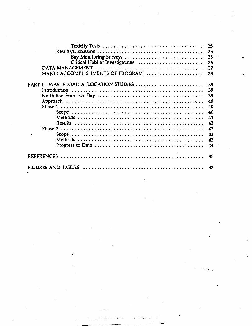
DATA MANAGEMENT •••.•••••.•••••MAJOR ACCOMPLISHMENTS 'OF PROGRAM

........

353535363738 "

PART II. WASTELOAD ALLOCAnON STUDIESIntroduction ••....••...South San Francisco BayApproach •...•.Phase 1

ScopeMethodsResults

Phase 2 •..••Scope, .MethodsProgress to Date

...

... '.

393939404040414243434344

REFERENCES .................................................... 45

FIGURES AND TABLES ..........' . 47

PROGRESS REPORT

This report summarizes the data coJlected in the San Francisco Bay 1991-1992 RegionalMonitoring Program. This is a progress report describing the work that has beencompleted to date. There were five different contracts written for the San Francisco BayRegional Monitoring Program that were funded by the Bay Protection and Toxic CleanupProgram. Each deal with different components of the monitoring program or wasteloadallocation studies: 1) sediment analysis, 2) bioaccumulation, 3) water column toxicity, 4)water column chemistry (organics) and 5) wasteload allocation. The Sediment Report andWater Column Toxicity Report are submitted with this summary as draft finals. All of thechemical analysis for the sediment study is not yet completed. The BioaccumulationReport is submitted in final fonn. Analysis of the water column samples for organicchemistry is not yet complete. The wasteload allocation studies are on a four year timeschedule. Progress on these studies is included in this report.

In addition, since the Regional Monitoring Program had many contracts and manysubcontractors in each contract (the sediment contract had six contractors) the finalreports do not analyze the data in a fuJly integrated fashion. We are currently trying tohire statisticians to thoroughly analyze all of the data coUected in the program so that wecan extract the most infonnation from the enormous amount of data we have. Anintegrated approach to data analysis is necessary in order to use this infonnation to guideour decisions in the future. Once aJl of the monitoring reports are final and an integratedstatistical analysis of the data is completed, a final version of this summary report wiJl beissued.

EXECUTIVE SUMMARY

This report i~ a summary of the progress to date on the San Francisco Bay Regional WaterQuality Control Board's Pilot Regional Monitoring Program (RMP). ,The RMP wasfunded by the Bay Protection and Toxic Ceanup Program. The main goal of thisprogram was to develop a regional monitoring and surveillance program that could' beused as a prototype in other bays and estuaries in the state. This was accomplished bysetting up monitoring programs and special studies to evaluate various techniques andprotocols used to sample water, sediment and tissue and to measure chemicalcontamination and toxicity. A second purpose of the program was to identify toxic hot

,spots in the Bay and in critical habitats (marshes, creeks and mudflats) arou,:,d the Bay.

This was a multi-media program in which chemical contamination and toxicity wasmeasured in water and sediments and bioaccumulation of contaminants was measuredin tissues. The program was divided into two major, monitoring programs two specialstudy programs and a data management component. ' The two monitoring componentswere the Bay Monitoring Surveys and the Critical Habitat Investigations.

In the Bay Monitoring Surveys, chemistry and toxicity was measured in the water andsediments at stations ranging from the South Bay to the Sacramento and San JoaquinRivers. The purposes of the Bay Monitoring Surveys were to: 1) monitor stations that ina longterm monitoring program would indicate spatial an4 temporal trends in toxicityand chemistry throughout the Estuary, 2) determine background for different basins inthe Estuary and 3) determine if there was toxicity or high levels of contaminants at Baystations. '

Critical Habitat Investigations were conducted primarily to determine if there were highlevels of contaminants, or toxicity " hot spots" in the marshes, mudflats or creekssurrounding the Estuary. Toxicity was measured in the sediments. Chemical analyseswas performed on sediment samples for a suite of metals and organics. Investigations oftoxicity in the water column of critical habitats focused on stormwater runoff in twosystems: 1) The Crandall Creek and Demonstration Urban Stormwater Treatment (DUST)marsh (DUST system) which retains stormwater in a freshwater marsh and 2) ArrowheadMarsh where stormwater is discharged into San Leandro Bay.

A special study was performed on a sediment gradient to: 1) determine which toxicitytests or type of toxicity tests (solid phase, elutriate, or pore water) could best distinguishbetween highly contaminated, moderately contaminated, and relatively uncontaminatedsites,2) evaluate the degree to which field replication increases the ability to distinguishbetween sites, 3) determine the effect of sample depth, 4) determine the relationshipbetween toxicity and factors that may effect toxicity including the levels of chemicalcontaminants, total organic carbon, grain size, ammonia and sulfides and 5) determine therelationship between toxicity test results and benthic community analysis. Shil1low aDddeep samples were collected at stations in Castro Cove, which has been historically

2

..

contaminated with" effluent from an oil refinery." Five field replicates were collected ateach station. Toxicity tests were performed on whole sediment, elutriates and porewater.Chemical analyses were performed on whole sediment and porewater. Samples forbenthic community analysis were collected from these stations. In addition, for anotherprogram, biomarkers were measured in fish e)(posed to the sediment in the laboratory.

A bioaccumulation study was petformed in order to: 1) describe the distribution of tracemetals and organics in organisms in the San Francisco Estuary, 2) determine thedifferences in contaminants in organisms collected in wet and dry seasons, 3) determinethe differences between mussels transplanted to shallow and deep water column depthsat the same station, 4) determine the effect of depurating sediment from the guts oforganisms on the contaminant levels in the whole bodies, 5) determine the optimumlength of e)(posure for transplant organisms and 6) determine the differences in uptakein three species, each with their own salinity t,?lerances.

To manage the data for the entire RMP a common format was developed for alllaboratories participating in the program. This allowed data to b~ more easily interpreted,analyzed and thoroughly checked for quality assurance. All laboratories in the programwere provided with consistent formats with QA programs integrated into the data inputsystem to insure accurate data entry. Data were generated at each of the laboratories andsent to EcoAnalysis for review.

For the sediment portion of the Bay Monitoring Surveys and Critical Habitat"Investigations, stations were identified where sediment was to,oc or showed elevated"levels of metals or organics (see results). Sediment was monitored at 15 stations baywideduring wet and dry seasons. For the Critical Habitat Investigations 32 sediment stationswere monitored. Preliminary studies and data from the monitoring programs indicatedthat: 1) for the amphipod test Eobaustaurius estuariys seemed more sensitive thanHyalella azteca and Rbepo)(jnius abronjus. even when a 28 day growth test wasconducted with HyaJelJa. 2) the Menjdja growth and survival test, using an elutriate, isnot sensitive and should not be used in a monitoring program, 3) diver cores seemed tobe the best way to collect undisturbed sediment samples, ne)(t best was the bo" core and4) chemical analysis indicated that the technique used for homogenizing samples was .adequate. Eohaustaurius seems to be an e"cellent organism for estuarine monitoringbecause it is tested in solid phase, is sensitive and can be tested at ambient salinity.

Only preliminary analyses have been completed on data from the gradient study butthese analyses seem to indicate that: 1) to,ocity was greater in deep samples, 2) thistmc.icity was not caused by high levels of ammonia or hydrogen sulfide, 3) tmc.icity testswere able to distinguish between stations, 4) field replicates were more variable thanlaboratory replicates,S) three laboratory replicates may be sufficient to distinguishbetween stations, 6) in the bivalve larvae test, porewater samples were much more taxicthan elutriate samples from the same sediment, 7) abnormality in the bivalve larvae testwas highly correlated with abnormality in the sea urchin test, 8) abnormality in neither

3

the urchin or bivalve test were correlated with the sea urchin fertiHzation test, and 9)sampling cores may be suitable containers for conducting amphipod tests.

For the water column por~on of the Bay Monitoring surveys, monitoring of organiccontaminants and toxicity was conducted at 15 and 12. stations, respectively, within theEstuary in June 1991 and April 1992.. The results of the organic contaminant monitoringwill be available in January 1993. Toxicity testing indicated statistically significant toxicityduring the first sampling event at two stations. Each station had significant toxicity in onetoxicity test. There was no significant toxicity in the sc;cond sampHng event.

Investigations of toxicity in the water column of critical habitats detected toxicity in boththe DUST system and Arrowhead Marsh following storm events. The DUST system wasfurther investigated to study the fate of toxicity in the receiving waters following stormevents of different intensity.

Bioaccumulation results indicated that: 1) bivalves at most of the stations within SanFrancisco Bay accumulated contaminant levels that were significantly higher than thecontrols collected at sites in more pristine locations outside of the Bay, 2.) stations in theSouth Bay, especially Coyote Creek, were significantly higher than the Central orNorthern Bay stations for DDT, PCBs, chlordane and PAHs,3) Stations in the South andCentral Bays were significantly higher than the North Bay for silver, 4) there were nosignificant differences in contaminant levels b~tween wet and dry seasons,S) there wereno significant differences between mussels deployed near the surface and those deployed

. near the bottom, 6) a small number of metals at each station were significantly different: between depurated and undepurated mussels, 7) an equilibrium appeared to be reachedin mussels during the three and four month transplants for copper, mercury, lead,selenium, and chlordane, but no equilibrium was reached for silver, PCBs and possiblyDDT after 120 days, 8) the patterns exhibited for DOTs, PCBs, and chlordanes fordeploment time experiments were similar indicating a similar source of these compoundsand 9) oysters and mussels exhibited similar concentrations of chlordane, DDT and PCBsbut PAHs differed and all metals differed greatly between the two species.

Although all of the data from the program has not been thoroughly analyzed, there are.already several major accompHshments of the RMP: 1) a Baseline Monitoring Program has .been established which will start in 1993, using the techniques and protocols evaluatedduring the RMP, to measure temporal and spatial trends in chemistry, toxicity andbioaccumulation throughout the San Francisco Estuary on an ongoing basis, 2) toxic hotspots were identified throughout the Bay and in critical habitat areas, 3) most of themarshes and mudfla.ts in the Estuary were surveyed for chemical contamination andtoxicity, 4) as the firSt step in setting up a statewide database, a format was generated fordata and laboratories in the Bay Protection Program were trained to use these formats sothat data could be easily checked for quality assurance, and integrated forstatistical.analysis,S) data generated in this program can be·combined with other data to generateApparent Effects. Threshold (AET) values for. San Francisco Bay and 6) problems in

4

,.'

identifying toxic hot spots and generating sediment quality criteria were identified andfuture studies were recommended to make the program more scientifically rigorous andprovide more certainty in the final results (see Recommendations for Future Studies).

Besides the Regional Monitoring Program, studies are also underway supporting thedevelopment of a wasteload allocation for South San Francisco Bay. In the first phase,a predictive water quality model was developed based on available water quality andhydrodynamic data, using the EPA model WASP4. The second phase includes collectionof time series of suspended sediment data to improve the ability to model transport ofpollutants associated with sediments.

~ .' -'

5

INTRODUCTION

The State Water Resources Control Board established the Bay Prot~tion and ToxicOeanup Program in April 1990 in order to implement Sections 13390-13396 of theCalifornia Water Cod~ (Chapter 5, Division 7). One of the requirements under the WaterCode is to develop an ongoing monitoring and surveilJance program in bays and estuariesof the state. The primary goal of the Pilot Regional Monitoring Program (RMP) was todevelop a monitoring and surveiHance program for the S~n Francisco Estuary that couldbe used as a prototype for the rest of the state. In addition, this program was designedto identify toxic hot spots in the Bay and in marshes surrounding the Bay and to collectdata that can be used to develop sediment quality objectives. In a second part of thisreport, the progress of wasteload aUocation studies is described.

,The RMP was primarily a monitoring program but special studies were also undertakento determine the best methods and stations to use to monitor the Estuary. A multi-mediaapproach was used in order to evaluate the ultimate, fate and effects of contaminants inthis complex estuarine system. Measurements of chemical contaminants, exposure oforganisms to these contaminants and toxic effects of contaminants on organisms were allmeasured. In the water column, chemistry, toxicity and bioaccumulation were measured.In the sediments, chemistry, and toxicity in both whole sediment and in pore water wereme'asured. In addition, biomarkers were measured in fish exposed in the laboratory tosediment samples synoptically collected for chemistry and toxicity.

Chemical measurements included a suite of metals and organics. At least three differenttoxicity tests were used to evaluate the effects of c()ntaminants in both water andsediment. Bioaccumulation was measured in three different species of sheUfish deployedin the water cplumn. These data will not only be used for the immediate needs of theBay Protection and Toxic Oeanup Program but also to determine backgroundconcentrations in the Estuary and to evaluate spatial and temporal trends in chemistry,bioaccumulation and toxicity.

,

Included in the program was a data management component. Under this part of theprogram, a common format was developed so that data could be more easily interpreted,analyzed and thoroughly checked for quality assurance. Although analysis is included .in this report for each component of the program, a thorough statistical analysisintegrating all portions of the program is currently being planned. All of the datapreviously mentioned are included in this report except for water column metals analysisand biomarker measurements, which were funded under another program and are on adifferent time sched.,I,.JJe. For a more thorough description of methods and results consultthe original reports.

, --

6

,"

PART 1. REGIONAL MONITORING PROGRAM

The RMP included two major monitoring components: Bay Monitoring Surveys andCritical Habitat Investigations. The purposes of the Bay Monitoring Surveys were to: 1)monitor stations that in a longterm monitoring program would indicate spatial andtemporal trends in toxicity and chemistry throughout the Estuary, 2) determinebackground for different basins in the Estuary and 3) determine if there was tmddty orhigh levels of contaminants at Bay stations. The Bay Monitoring Surveys includedchemical and toxicity measurements in the water column and in the sediment. In thewater column, metals were analyzed at 27 stations, organics at 14 stations and toxicity at12 stations. Sediment chemistry and toxicity were measured at 15 stations.Bioaccumulation in shellfish was measured at 8 stations. Each group of stations was asubset of the 27 water column stations. However some sediment stations, althoughlocated in the same general vicinity as the water column stations, were changed due tothe composition of the sediment. The stations ranged geographically from the South Bayto the Sacramento and San Joaquin Rivers.

Critical Habitat investigations were conducted primarily to determine if there were highlevels of contaminants or toxicity n hot spotsn in the marshes and mudflats surroundingthe Estuary. Sediment chemistry and toxicity were measured in most critical habitatsaround the Estuary, except for the South Bay which has been extensively monitored inthe recent past. Water column toxicity was measured in several of these marshes,although most of the work relating to water column toxicity concentrated on the effectof runoff on the Demonstration Urban Stormwater Treatment (DUST) marsh in the SouthBay and Arrowhead Marsh in San Leandro Bay.

Special studies on sediment toxicity and bioaccumulation were also conducted and aredescribed in those sections below. In addition, a data management component wasincluded so that all of the data would be consistent and could be integrated for qualityassurance and statistical analysis.

7

SEDIMENT

Study Design

Several preliminary studies were conducted for the sediment monitoring programs todetermine: 1) the most appropriate amphipod species and endpoints to use in an estuarywith a wide range of salinities and 2) a fine grain reference site. These studies arediscussed in more detail in the Sediment Report. Tests exposed the amphipod HyaJeIJaazteca to two freshwater reference sediments (Del Valle Reservoir and Lake Mendocino)and two 'contaminated sediments (Coyote Creek and Mayfield Slough). The duration ofthe ~ests were 14 and 28 days. Endpoints were 14 day survival and for the 28 day testthree growth measurements. Eohaustaurius estuarius was exposed to two estuarinereference (Brazil Beach in Tomales Bay, and Drakes Estero) and two estuarinecontaminated sediments (Oakland Inner H.arbor and Castro Cove). The duration of thetest was 10 days and the endpoint was survival. In addition, both HyalelJa andEohaustaurius were exposed to low salinity sediments (3-4 ppt) from Lake Mendocino,Blanco Drain, Mayfield Slough and Stockton Harbor to determine if Eohaustayrius couldbe used at low salinities. The results of these studies indicated that 1) the mostappropriate amphipod test to use for the sediment monitoring programs was the 10 dayamphipod test, using Eohaustaurius and measuring survival, 2) Eohaustaurius could berun in estuarine sediment down to 4 ppt but it had low survival in freshwater sedimentthat was salted up and 3) the best fine grain reference site out of those tested was BrazilBeach in Tomales Bay. However, after testing with Brazil Beach sediment showed

. toxicity in consecutive studies, including the first Critical Habitat survey, the site was.c~anged to Marconi Cove in Tomales Bay. Still, throughout the study Marconi Covesediments exhibited sporadic toxicity. .

Additional samples were collected at Drakes Estero, Tomales Bay, Oakland Inner Harbor,Del Valle Reservoir, Mayfield Slough, Lake Mendocino and Coyote .Creek for porewater analysis. Samples were taken with a sampling core. Pore water was extracted withsyringes inserted at different depths. Pore water was analyzed for ammonia, nitrite plusnitrate, phosphate, dissolved oxygen,silicate, manganese, silver, iron and lead.

Bay.Monitoring Surveys

Composite samples of the depositional layer were collected at 15 stations duringthe dry season (August 1991) and 14 during the wet season (April 1992) (Figure 1and 2; Table 1 and 2). A fine grain sample could not be collected at Davis Pointduring the ~~t season. The depositional layer was defined by being brown incolor, loosely compacted and lacking the smell of hydrogen sulfide. Because of thehighly dynamic nature of the San Francisco Estuary, due to wind, tides andcurrents, sediment is constantly resuspended and redeposited. In this program wedecided not to sample the top 2 em, as is done in most sediment surveys, becausewe felt that in most areas that dept~ was constantly in a state of flux. To truly

8

.'

characterize a site we decided to sample a deeper layer. We sampled down to theinterface where the e>dstence of hydrogen sulfide was evident. The sulfide layerwas not sampled because of possible confounding effects in tmdcHy rest results.

Sediment was homogenized and analyzed for concentrations of metals andorganics and for to>dcity. Three toxicity tests were used in the dry weather run.These were the solid phase 10 day amphipod test using Eohaustaurius and twoelumate tests, the bivalve larvae test measuring development, and the MenidiaberyJlina test measuring growth and survival. The Menidia test was deleted fromthe wet weather run because after much testing it proved to be less sensitive thanthe other tests.

Critical Habitat Investigations

Composite samples of the depositional layer were collected at 32 stations locatedin marshes or mudflats around the Estuary (Figure 3; Table 3). Four separatesurveys were conducted, each in a separate part of the Estuary. The sediment wasanalyzed for metals and organics and tested (or to>dcity using the same threeto>ddty tests used for the Bay Monitoring samples. However, several tests fromfreshwater stations were conducted using the 7 day test for~magna, whichmeasures reproduction.

Gradient Study

The main purposes of the gradient study were to: 1) determine which toxicity testsor type of toxicity tests (solid phase, elumate, or pore water) could best distinguishbetween highly contaminated, moderately contaminated, and relativelyuncontaminated sites, 2) evaluate the degree to which field replication increasesthe ability to distinguish between sites, 3) determine the effect of sample depth, 4}determine the relationship between toxicity and factors that may effect toxicityincluding the levels of chemical contaminants, total organic carbon, grain size,ammonia and sulfides and 5) determine the relationship between to>dcity testresults and benthic community analysis.

Castro Cove was chosen as the study site. There were four station locations on adistance gradient away from "an historic outfall from a petroleum refinery (Figure4). Station locations were chosen based on historic data and a reconnaissancesurvey. At three of the four stations, including the most contaminated and theleast contaminated, samples were taken at two depths (the depositional layer,referred to as shallow, and one foot, referred to as deep). The depositional layerat station GD23, the third station from the source, could not be sampled becauseof an intense infestation of tube worms at the station that was not there duringthe reconnaissance survey five weeks before. In addition, sediment from Cardnletin Puget Sound, Washington was also sampled at two depths and used as an

".

· additional clean control for all of the toxicity tests, including pore water tests, inthe study. A full chemical analysis was conducted on the sediment and pore waterfrom Carr Inlet. At all seven stations (each depth was considered a separatesta,tion) five field replicates were collected. Each field replicate was a compositemade up of at least five cores.

Twelve liters of sediment were collected (or each field replicate and homogenized.Sediment was then separated for pore water or whole sedimenVelutriate analysis.Whole sediment was analyzed for metals, organics, grain size and total organiccarbon. The 10 day amphipod test, using Eohaustaurius was conducted withwhole sediment. In addition, speckled sanddabs, Citharicbthys stigrnaeus , wereexposed to this. sediment for 60 days in the laboratory, after which a series ofbiomarkers were measured (these results will be reported in a separate report).The bivalve larvae development test was also conducted on an elutriate of thesediment using the same techniques that were u'sed in the monitoring portion ofthe program.

Pore water was squeezed from the sediment and used for chemical analysis andtoxici ty tests. Pore water was analyzed for organics, metals, ammonia, sulfides, pHand dissolved oxygen. Pore water toxicity tests measured: 1) bivalve larvaldevelopment, 2) sea urchin fertilization, development, cytologic and cytogeniceffects, 3) nematode broodsize and mutagenic effect and 4) bacterial mutagenicity.In addition, a. different pore water sampler was used to extract p.ore water atdifferent depths. Concentrations of ammonia, hydrogen sulfide, dissolved oxygen,nitrite plus nitrate, silicate and manganese were measured in each sample.

In addition to chemical measurements, toxicity tests and biomarker measurements,samples were collected at each of the four station locations (G010/20, G011/12,G023 and G011/22) for benthic community analysis. Five field replicates werecollected at each location.

A dilution experiment was also conduc.ted on sediment from the gradient study todetermine: 1) whether Eohaystaurius or Rhepoxjnjus was more sensitive to CastroCove sediments and 2) if salinity effected toxicity to EohaustaUrius. The 10 day .amphipod test was performed for both species on dilutions. of Carr Inlet and a mixof G010 and G020 sediments (sediments from the most toxic site). Sediment wasmixed to achieve six concentrations: 100, 80, 60, 40, 20, and 0 % . Eohaustuatiyswas tested at 10 and 25 ppt. Rhepoxjnjus was tested at 28 ppt.

10

"

Methods

Sampling

Sediment was sampled by four different methods: 1) a modified Gray-Ohara boxcore, 2) diver operated cores, 3) diver operated scoops, and 4) hand held scoops.The method used depended on the environment being sampled. For the BayMonitoring Surveys the box core was always used. For the Critical HabitatInvestigations one of the other three methods was used depending on whether thesediment was exposed or underwater. Diver operated cores or scoops were usedif the sediment was underwater. Hand held scoops were used if the tide was outand the sediment was not underwater. Diver operated scoops were considered theleast effective in maintaining the integrity of the top layer of sediment. Thesewere used for the first of four Critical Habitat Investigations but after this wereonly used for collecting reference sediment. For the Gradient Study, except forCarr Inlet sediment, only ,diver cores were used. Diver cores were the best methodfor mai~taining the integrity of the top layer of sediment.

All sampling equipment was made of Teflon, polyethylene, or polycarbonate andwas pre-cleaned and protectively packaged prior to entering the field. Newsampling equipment, except for the sampler, was used at each station. Allsampling equipment (excluding the sediment sampler) was cleaned by: a ~day

soak and wash in Micro brand detergent, 3 Milli-Q water rinses, 3 deionized waterrinses, a 3-day soak in 10% HCL or HN03, 3 Milli-Qwater rinses, air dry, 3petroleum ether rinses, and air dry. The sediment sampler was cleaned prior toentering the field by: a vigorous Micro brand detergent wash and scrub, a tap­water rinse, a 10% HCL rinse, and a petroleum ether rinse. To avoid cross­contamination, the sediment sampler was thoroughly cleaned between samplingat each station with a seawater rinse, scrubbing with Micro brand detergent, aseawater rinse, 1% HO rinse and a methanol rinse. .

The San Francisco Estuary is a highly dynamic system. Wind, currents and tidesconstantly resuspend and redeposit sediment. Organisms reburrow and areexposed to deeper sediment when it is resuspended. In most sediment studies, the .top 2 cm of sediment is sampled. A decision was made in this study that the top2 em was not deep enough to characterize a site in this Estuary. Yet, at that timeit was unclear how much effect ammonia and hydrogen sulfide would have ontoxicity tests if we sampled the sulfide layer. Also, it was felt that the mobilizationof sulfides could create artificial conditions by either extracting metals from thepore water during homogenization or releasing metals during bioassay exposure.For these reasons the decision was made to measure as deep as possible withoutsampling the sulfide layer. For all studies, except the deep samples in the. GradientStudy, the depositional layer was sampled. This layer was characterized by oeingbrown in color, relatively noncompacted and lacking the smell of hydrogen sulfide.

11

This layer ranged, depending on the site from 1 cm to 20·cm. The average depth{or the'Bay Monitoring Surveys was 10 cm.

Most samples were a composite of grabs. The amount of grabs varied from 1 to20 depending on the depth of the depositional layer at that site, the greater thedepth the fewer the grabs. The Bay Monitoring Surveys averaged 6 grabs.Sediment was placed in a tub and homogenized. , It was then divided up for thevarious types of analyses conducted in the study.

For the Gradient Study whole sediment was sampled from the depositional layerand to a depth of one foot using a diver core. Pore water was coJlected from eachsample. For every field replicate homogenized sediment was divided into sedimentthat would be used for whole sediment analysis and sediment that would be used{or pore water analyses. The sediment ~o be used for pore water analyses wassqueezed by a whole core squeezing method developed by Bender et al. (1987).This method utilizes mechanical force to squeeze pore water from interstitialspaces. The pore water was then divided for the various types of chemicalanalyses and toxidty tests.

A second method was used (or sampling pore water at various depths. Thismethod used a pore water squeezer to coJlect dissolved «0.45um) pore watersamples, in replicate, from depths of 0, 1, 2, 4, 6, 8, 10, 14, 18, 22 and 26 em.Filtered water samples were drawn directly into acid-cleaned polyethylene (LDPE)syringes; the syringe contents were filtered through a 0.45um teflon syringe filterinto an add-cleaned LOPE bottle. The samples were then addified with sub­boiling quartz distiUed (2x) adds in a trace element clean laboratory. SamplescoUected by this technique at Drakes Estero, Tomales Bay, Oakland Inner Harbor,Del Valle Reservoir, Mayfield Slough, Lake Mendodno and Coyote Creek wereanalyzed for ammonia, nitrite plus nitrate, phosphate, dissolved oxygen, silicate,manganese, silver, iron and lead. Castro Cove samples were also collected by thismethod,' These samples were analyzed for ammonia, hydrogen sulfide, dissolvedoxygen, nitrite plus nitrate, silicate and manganese.

Organic Chemistry

Organic contaminants 'were measured in sediments and pore waters.Concentrations of PAHs, PCBs, and chlorinated pesticides in sediments weremeasured with established techniques. All sediment values are reported in dryweight. Concentrations of the same compounds in pore waters were measuredwith experimental techniques, due to the sensitivity limitations of the smallvolumes available. '

, --Sediments were freeze-dried, mixed with kiln-fired sodium sulfate, and soxhlet­extracted with methylene chloride. The methylene chloride was then replaced by

12

•

;~,

hexane. Lipids were removed by florisiJ-column chromatography. Sedimentextract volumes were concentrated to approximately 1-4 ml and analyzed by bothelectron-capture gas chromatography (Varian 3400 GC with 8100 autosampler) andby GC/MS (Saturn II, also with 8100 autosampler).

Pore water samples in the gradient study, about 50 ml, were extracted three timeswith methylene chloride in a separatory funnel. The methylene chloride wasreduced and replaced by hexane. Pore water extract volumes were reduced to 5-10microliters before analysis by GClECD and GC/MS to achieve the necessarysensitivity.

For total organic carbon analysis, aliquots of freeze-dried or oven-dried sedimentswere prepared by agitation in IN HO, repeating the process until there was nofurther evolution of carbon dioxide. After centrifugation and decanting, sedimentswere rinsed with Milli-Q treated water, centrifuged again, and dried at 60 degrees.Subsequent steps in the analysis were undertaken by using established methods(Froelich, 198~ Hedges and Stern, 1983; and suggested procedures of themanufacturer). The methods are comparable to those of the recent validationstudy of the EPA method MARPCPN conducted by the Chesapeake BiologicalLaboratory of the University of Maryland.

Metals Chemistry

Two different methods were used to prepare whole sediment samples for chemicalanalysis. The first involved a near total (aqua regia) digestion consistent with therecommended procedures of the United States Environmental Protection Agencyfor sediment analyses (EPA, 1974). This procedure provides a conservative measureof trace element concentrations in sediment and can be used to compareconcentrations with historical measurements and numerical sediment guidelinesand standards. The second procedure extracted "biologically available" traceelements by using a dilute acid (0.5 N Ha) extraction procedure (Flegal et aI.,1981). This procedure was developed for the State Water Resources Control Boardto monitor trace element concentrations in marine sediments and wastewater .sludge. Research has indicated that this extraction method is consistent with theextraction for acid volatile sulfides (Ditoro, 1990).

The first method of digestion was used to prepare samples that were analyzed foraluminum, chr9mium, cobalt, copper, iron, lead, magnesium, manganese, nickel,phosphorus, silver, vanadium and zinc. The second method was used to preparesamples that were analyzed for aluminum, cadmium, iron, magnesium, manganese,phosphorous and vanadium. Elemental concentrations were measured by'Grar-l:li!efurnace atomic absorption spectrometry (CFAAS), flame atomic absorptionspectrometry, (MS), and/or inductively coupled plasmCll 21tomic <emission

13

spectrometry (ICP-AES). All samples were measured in duplicate.

Total arsenic, mercury, and selenium were analyzed by American EnvironmentalCorporation. Methods used for these metals were: arsenic (EPA Method 7061),mercury (EPA Method 7471) and selenium (EPA Method 7741). The instrumentused for detection was in all cases a GFMS. Tributyltin was analyzed by Toxscan,Incorporated using a gas chromatograph with a flame photometric detector. Allmetals values for the project are reported in dry weight.

Pore water samples were conce~trated with an APDC/DDC organic extraction,which was based on the procedures described ,by Bruland et al. (1985). Thismethod was necessary because of the small volumes of pore water that couId beextracted. The total dissolved « 0.45um) concentrations of pore water sampleswere measured with microtechniques based on procedures used to measure totaldissolved trace element concentrations in surface waters in the San Franciscoestuary (Flegal et aI., 1991). Therefore, this set ofdata may be compared to othermeasurements of trace element concentrations in surface waters. Pore watersamples were analyzed for cadmium, cobalt, copper, iron, lead, manganese, silverand zinc. Concentrations were measured by GF~S and by ICP-AES.

Additional pore water measurements collected at various depths and analyzed fordissolved ammonia, phosphate, silicate, and nitrate plus nitrite used the proceduresdescribed by Gieskes and Peretsman (1986).

Toxicity Tests

For the first Bay Monitoring Survey and the Critical Habitat Investigations threesediment toxicity tests were performed: the amphipod, bivalve larvae and Menidiatest. The 10 day amphipod test measuring survival was performed on wholesediment (ASTM, 1992). The amphipod Eohaustaurius estuarius was used so thatall tests could be conducted at ambient salinity. R~epoxinius abronjus was testedat a subset· of stations to compare tJ:te sensitivity of the two species. Control

. (hoJ:T\e) sediment was used in all tests. In additi.on, fine grain sediment fromTomales Bay was run as a reference sediment.

Elutriate tests were performed with bivalve larvae measuring development andwith the inland silverside, Menidia beryJ)jna, measuring growth and survival. TheMenjdja test was used because 1) it has been shown to be sensitive in watercolumn tests, 2) we wanted to determine possible toxic effects on fish and 3)Menjdja has a broad salinity tolerance. Elutriates were prepared by mixingsediment with dilution water in a sediment-to-vvater ratio of 1:4 by volume(EPNACOE, 1991) and shaken vigorously for 10 seconds (Tetra Tech, 1986). Theone liter mixture was allowed to settle for 24 hours and then carefully decanted

14

into al one liter Erlenmeyer flask.

Tmdcity tests with bivalve larvae were conducted following ASTM guidelines(ASTlVl, 1991) with adaptations for elutriate testing given in fthe lPuget SoundProtocols (Tetra Tech, 1986). Pacific oysters, Cr855sostma gipi, we~ used in alltests except the third marsh run, which was run in IRcember when spawnableoysters were unavailable. At that time, oysters were replaced by bay mussels,Mytilys edyJis. Toxicity tests measuring growth and survival in Menidia ber:y1linafollowed the EPA protocol (Weber et at, 1988). A subset of stations were alsotested measuring growth and survival in the topsmelt Atberino!2§ affinjs(Anderson et aI., 1990). Both tests are growth and surviv.mI tests in which younglarvae are exposed to test solution for" days. However, AtherinQ~ is a localspecies and Menidia is imported. For the second Bay Monitoring Run, which wasthe last monitoring run to be conducted, larval fish tests were dropped from thetests because they were insensitive in .the previous tests. Several! ~ests fromfreshwater stations were conducted using the ., day test foB'~ Dl.AtPJAmeasuring reproduction described by Nebeker et a1. (1988).

In the gradient study both the amphipod test using Eohaustaurius and the elutriatebivalve larvae test were performed on test sedimenl Protocols were the same asdescribed above. In addition, other toxicity tests were performed on wholesediment and on pore water. The amphipod test using Eohauslauriys wasperformed within cores used to collect sediment in the field. At three stations inthe gradient study, five separate core tubes (10 em diameter) were taken in to thefield and used to sample sediment at each field replicate (5 per station) to a depthof 10 em. These cores were capped, top and bottom, in the field with 10 em ofoverlying water which was retained throughout transport. The actual collectioncores were then used as the test containers.

Several toxicity tests were performed in pore water extracted from the sediment.The bivalve larvae test was performed using the same methods as in the elutriatetests (ASTM, 1991). The echinoderm fertilization test was conducted according tomethods described by Anderson et a1. (1990). Development scoring, cytogenicanalysis and cytologic analysis were all conducted on the same samples. Cytogenic·andcytologic evaluations were conducted according to the methods of Hose andPuffer (1983). The echinoderm, StrongylocentTotus~ was used for allechinoderm tests. A bacterial mutagenicity test was conducted on Salmonellaaccording to the methods of Kado et aI., (1983, 1986). This assay is a simplemodification of the Salmonel1a1microsome test of Ames el a1. (1975). The nematode(C. elegans) broodsize and mutagenicity assay was performed using methods ofRosenbluth et al. (1983) and Anderson et .mI. (submitted MS). This test assessesalterations in broodsize in the Fl and F2 generations as well as mutations i!l_ aspecific target region of the genome. -

15

All toxicity tests had five laboratory replicates except in the gradient study. Afterstatistically analyzing data from the previous studies, we determined thatlaboratory variability was so low that using three laboratory replicates instead offive did not effect the ability to distinguish between stations. Field variability wasexpected to be much greater than laboratory variability, therefore, five fieldreplicates were coUected at each station. Positive reference toxicants were used forall tests. Dissolved oxygen, pH, temperature and ammonia were monitored in thetests. Grain size was also measured to evaluate the amphipod tests. In thegradient study sulfides were also measured.

Benthic Analysis

For the gradient study five replicate cores.(.018m'lcore) were collected from eachof the four main gradient stations (GD10/20; GOn/21, G023 and G011122). Coreswere immediately screened through 5mm mesh, and fixed in 10% formalin.Samples were transferred four days later into 10% isopropyl alcohol, sorted,identified to the lowest possible taxon, and counted under a dissecting microscope.

Results/Discussion

A thorough, integrated, statistical analysis of the sediment results has not been completed.Although toxicity test results are complete, all of the chemical analyses are not.Therefore, toxicity test results are described, but the results for chemical analysis and theintegration of chemical analysis with toxicity test ~sults is considered preliminary. Theresults for each study and each type of analysis are discussed in that section.

Bay Monitoring

Organic Chemistry

For sediment samples from the Bay Monitoring surveys, PAH concentrationsranged from 81 to 6300 nglg with a median value of 810 nglg. A review ofPAH residue data previously obtained from San Francisco Bay by the Statusand Trends program of NOAA (NOAA, 1988) provided a mean (arithmetic)of about 2.5 ppm dry weight.

In al~~~t all samples, the combustion profile dominated the petroleumprofile. In only one of the Dumbarton Bridge samples and one of theRedwood creek samples did most of the PAHs derive from petroleum ratherthan combustion sources. Combustion residues derive primarily from "tfieatmosphere (the principal local source is probably automobile exhaust) and

16

surface runoff during rainstorms. PAH residues that derive (rom petroleumand petroleum products are generally from spills,· those released intodisposal systems and as components of surface runoff.

Metals Ch~rnistry

In general, distributions of the chemicals measured could be classified intotwo principal groups~ These were 1) the elemenb which sh9w someanthrop~genic enrichment in some location~ (Ag, ~~~ Cu, lPb, and ?r') and2) those ~ith less pronounced perturbations (Co~ Cll', Ni, an~ V). this wastrue for both Bay and Critical Habitat surveys.' .

An trace elements, except V, showe~ a significant difference with season atseveral stations. However, when statiOI)S w~re poole" there was nosignificant diff~rellce between seasons. .

In order to evaluate the potential for toxiclty based on sediment chemistry,trace element concentrations were compared to concentrations which causedtoxic effects in previous studies and the enrichme~t of the element relativeto its natural abundance. The Effects Range-Low (ER-L) and Effects Range­Median @R-M) values of Long and Morgan (1990) .~. presented to proVjQea basis for evaluating the potential adverse effects 'of contaMination. Theaverage continental crustal abundance (CA) of each element (Lof, 1987) hasbeen included to provide a measure of the enrichment or depletion of eachelement relative to its average natural concentratio~. Figures 5-12 showconcentrations of trace elements (Ag, Cd, Cr, Cu, Ni, ~, arid Zn) measuredin the Bay Monitoring runs along with ER-L, ER-M and CA values. Table4 illustrates the mean, standard deviation, median, maximum and minimumconcentrations for trace elements in the Bay Monitoring surVeys.

The ER-L yalue of 35 ppm lead was exceeded by stations BB31 (OysterPoint), B020 (petaluma River), and B051 and B052 (Napa River) duringboth wet and dry monitoring runs. Lead concentra~ons in sediments at .BCSO (Stauffer) exceeded the ER-L during the wet weather run. BC10(Verba Buena Island), BC30 (Richardson Bay), BD40 (Davis Point), B030(point Pinole), BF10 (pacheco Creek) and BF20 (Grizzly Bay) exceeded theER-L during the dry weather sampling. The highest concen~ration of leadin the bay sediments was at Davis Point (B040), where the leadconcentration was equal to the ER-M of 110 ppm.

Most stations which exceeded the ER-L values for lead also exceeded theER-L vaJu~s for zinc. This is reflected by the highly significant correlationbetween lead and zinc concentrations. Sediment concentrations of zinc and

17

"--:-... ...._ ... ~ ·w.·.·

.... _- -..

lead in San Francisco Bay are greater than their average crustal abundances.

Only Davis Point had silver concentrations which exceeded its ER-L valueof 1 ppm. But, all stations sampled were enriched with respect to theaverage crustal abundance of silver, some as much as ten-fold.

The only station that exceeded the ER-L value for copper was a boat yardin Richardson Bay (BC30). Copper concentrations were four times higherthaJ1 samples collected outside of the boat yard (BC31) during wet weather.These concentrations appear to be due to contamination of sediments due.to boat yard activities.

None of the Bay sediments exceeded the ERL for cadmium (5 ppm). Thatvalue is 50 .times greater than the ,average crustal abundance of cadmium.The ERL for chromium was exceeded at many stations and the ER-M fornickel was exceeded in sediments at every station. The ER-M for nickel ismuch higher than its,average crustal abundance.

The chemical concentrations of replicate samples collected from eachhomogenate were highly precise. This indicates that the homogenizationof composite samples at each station was successful.

Toxicity Tests

Ampbjpod tests • Due to sporadic toxicity in the fine grain referencesediment, it was difficult to determine what actually constituted a toxicresponse. In the dry weather Bay Monitoring survey the reference site wasnot significantly different than the controls but in the wet weather surveyit was. Con,tractors statistically compared test sediment to both home andreference sediment (Table 5). This approach makes sense except that someof the response of the organisms in test sediment, when statisticallycompared to home sediment due to the lack of an adequate referencesediment, may be due to fine grain size rather than toxicity. In thissummary, since these data are being used to identify toxic hot spots, aconsistent 25% effect level compared to home sedimeilt will be used toidentify stations that were toxic. This issue is more thoroughly discussed·in the Recommendations for Future Studies section.

In the"August 1991 dry weather Bay Monitoring survey, stations thatshowed a 25% reduction in survival compared to home sediment included:

BA20· Extrem'e South BayBA30 • Dumbarton BridgeBA40 - Redwood CreekBB31 - Oyster Point Marina

18

8C30 - Richardson Bay, Anderson's Boai YardBD20 0 Petaluma River, Lt. 188051 0 Napa River, West Bank, Mare IslandBFIO - Pacheco CreekBF20 0 Grizzly lBaly

These stations were the same stations that had significantly less survivalthan both the home and reference sediment in statistical tests.

In the April wet weather Bay Monitoring survey stations showing a 25%reduction compared to home sediment included:

18A20 - Extreme South Bay .lBA30 - Oumbarton Bridge18A40 - Redwood CreekBB31 0 Oyster Point MarinaBC31 - Richardson Bay, outside channellBCSO - StauferB020 - Petaluma River, Lt. 18B052 - Napa River, East Bank, VallejoBF20 - Grizzly BayBG21 - Sacramento River in Sherman Lake

These stations and BFI0 (pacheco Creek) and BC1l0 (Verba Buena Island)had significantly less survival than home sediment in statistical tests.

In addition, Rhepoxiniu5 was exposed to sediment from BA20, BA40, BB3O,BC30, BCSO and BD40 for the dry weather run. Using the same methodthat was used for Eohaustaudus to determine tmdcity, only BA20, ExtremeSouth Bay, was toxic. This was also the only station with significantlyreduced survival compared with both the reference site and controls (fable6).

Grain size was significantly correlated to survival for Eohaustaurius but notfor~. However, grain size may not be all that is directlyeffecting the amphipods. Sediment with larger grain size probably also hasa Jower concentration of contaminants. Ammonia did not exceed 6 ppm in .any test, therefore, it is not expected that ammonia contributed to toxicity.

Differences in survival were not significant for tests run with sedimentscolJected in the wet weather versus those collected in the dry weather run.This is consistent with the results of chemical analysis, which showed nosignificant differences in trace metal concentrations between pooled wetand dry weather samples.

Daphnia Test - The~ test was run on samples from stations BG21and BG31. There was no significant difference in reproduction when

19

, ... <" "',, .... -:

compared to sediment from Lake Mendocino, the freshwater. reference site(Table 1).

Bivalve Larvae Tests - For the August- 1991 dry weather run,' BA40(Redwood Creek) and BF 10 (pacheco Creek) were significandy differentthan seawater controls. Reference sediments were not tested at the sametime as test sediments for this run. For the April 1992 wet weather runB020 (petaluma River,Lt. 18), BG2l (Sacramento river at Sherman Lake) andBG32 (San Joaquin River at KimbaJl Island) were significantly different thanboth the seawater control and the reference sediment. See Table 8 for themeans and standard deviations at each station.

Menidja Tests - The Menjdja test was only performed on sedimentscollected in the August 1991 monitoring run. There were no samples thatwere significantly different than either the seawater controls or thereference sediment (Table 8b). This test was dropped from the April 1992monitoring run because of its lack of sensitivity.

Critical Habitat Investigations

Organic Chemistry,

In the sediment samples from this part of the study PAH concentrationsranged from 35 to 9,100 Jlglg, With a median of 1,200. Higher'concentrations in these areas may reflect both proximity to runoff inputsources and higher organic carbon/silt levels~

Metals Chemistry

Figures 13-21 show concentrations of trace elements (Ag, Cd, Cr, Cu, Ni, Pb,and Zn) measured in the Critical Habitat surveys along with ER-L, ER-Mand CA values. By far the highest metals concentrations were found atPeyton Slough (MF22). The concen~ration of copper in this sample .exceeded the TILC (2.5 glkg). The concentration of zinc (4.39 glkg)approached the TILC (5.0 glkg). The concentration of cadmium was thehighest found in the entire study (1951 mWkg). All of these concentrationsfar exceed the ER-M for these metals. Yet, there were no toxic effects in thebivalve ·larvae test, a test that is particularly sensitive to metals. In theamphipod test, although there was significant toxicity, swvival was 60%.This illustrates the importance of being able to estimate the bioavailablefraction of metals. Additional analysis is being conducted on tms sample.Historically the site was used for copper slag. See the Recommendationssection for a further discussio.n of this issue.

20

«

Sediments from San Leandro Bay (MBll) and Cordinices Creek were abovethe ER-M levels {or lead (110 ppm) and zinc (260 ppm), as well as the ER-Lfor copper (70 ppm). Sediments from Cordinices Creek also exceeded theER-LvaIue for silver (1 ppm). Silva Island Marsh (MC61) exceeded the ER­M value for lead and the ER-L value for zinc. Emeryville Marsh exceededthe ER-M value for zinc and the ER-L value for lead. All of these sampleswere collected near urban storm drains.

In Tomales Bay, sediment concentrations exceeded the ER-M value forchromium (BOppm) and the ER-L value for nickel (SO ppm). In fact, thechromium and nickel concentrations of sediments in Tomales Bay were thehighest in the entire data set. Yet, chromium concentrations were belowthe average crustal abundance. Serpentine deposits in the area mayaccount for elevated levels of chromium and nickel, although almost allsediments sampled in the RMP exceeded the ER-M for nickel (Fig.3-A-4 andFig.3-B-4). The ER-M for nickel is well below its average crustal abundance.

Toxicity Tests

~ - In tWo out of the four marsh surveys, survival in thereference sediment was poor. Therefore, the same method for reportingtoxicity as was used in the Bay Monitoring runs will be used for the CriticalHabitat Surveys. Table 9 shows mean survival and statistical analysis foreach station, comparing results from each station to both the home andreference sediment.

Stations showing a 25% reduction in survival compared to home sedimentincluded:

MF10 - Boynton Slough ClMF11 - Boynton Slough C3MF12 - Boynton Slough C4MF20 - Hill Slough, below bridgeMF21 - Hill Slough, above bridgeMF22 - Peyton Slough, back end of sloughMD31 - Tolay Creek mouthMD32 - Napa Slough at bridgeMD33 - Sonoma Creek at TubbsMD34 - Sonoma Creek at bridgeMC30 - Emeryville Marsh at EBMUD storm drainMCSO - Corte Madera Marsh S of Industrial Rd.MD20 - Gallinas Cr. at John F. McInnis County ParkMD21 - Novato Creek at Lock

21

Regression analysis indicated that the percent sand of s~mples from criticalhabitat sediments accounted for little of the variability in survival for theEohaustaurius tests.

Daphnia Test - The Daphnia test 'was run on stations MF10 (BoyntonSlough Cl), MFll (Boynton Slough C3), MF20 (HiJI Slough, below bridge)and MF21 (Hill Slough, above bridge). The only station that showed asignificant decrease compared to reference sediment, which had highreproduction, was MF20. The Daphnia test was less sensitive than theamphipod test in detecting toxicity.

Bivalve Larvae. MeJiidja and Atherlnops Te~ts • Results for these three testsare summarized in Table lOa and lOb. The reference sediment was toxic intwo out of the four marsh runs for the bivalve larvae test. These were thesame samples that were toxic in the amphipod test. Since the runs wherethe reference site was toxic were the only runs where test sample toxicitywas observed, only samples that were significantly more toxic than seawatercontrols will be listed. These stations for the bivalve test are:

MF10· Boynton Slough, Cl,MFll • Boynton Slough, C3MF12 - Boynton Slough, C4MF13 - Chadbourne Slough, CR2MF23 • Peyton Slough, mouth of sloughMD10 - Miller Creek at Las Gallinas dischargeMOll - Miller Creek upstream from discharge at fenceMC6l - Silva Island Marsh at Seminary Dr. storm drain

MF20 and MF21 were not tested.

The only sample that was toxic to Menidia, besides the Lake Mendocinoreference sediment, was MC6l (Silva Island Marsh at Seminary Dr. stormdrain). Atherinops was used to test for toxicity on' the 8 Suisun Marshstations. Only MF21 (Hill Slough, above bridge) was to?dc to this species. .Due to the general insensitivity of the elumate fish tests they were droppedfrom the final Bay Monitoring survey.

Gradient Study

Organic Chemistry

- "

The highest concentrations of PAHs in the entire Regional MonitoringProgram were measured in Castro Cove, At the station closest to the

22

«

source, PAH concentrations were 21 and 8.4 ppm, geometric means, in deepand shallow sediments, respectively. At the intennediate stations thegeometric mean total PAHs in deeper sediments were 1.1 and 0.9 ppm, andat the Point Pinole Pilings (PPP) station, tile station farthest from ihe source,concentrations were 0.6 and 0.9 in deep and shallow sediments respectively.With the e)(ception of PPP, the PAHs in the Castro Cove stations derivedprincipally from petroleum, and were associated with comple)( mixtures ofother petroleum hydrocarbons. The "fingerprint" ofPAH compounds in thesurface sediments at PPP was the typical combustion profile characteristicof most arees of San Francisco Bay.

In the gradient study, contaminant variables were highly and significantlycorrelated with each other, and with related variables such as the organiccarbon and nitrogen content. Thus mortality in the amphipod test wassignificantly correlated with all of the contaminant variables measured.Development of. oyster larvae in the elutriates, however, was mostsignificantly associated with the organic carbon and nitrogen content of thesediments, rather than with the contaminants, suggesting that variablessuch as small particulate material in the elutriate might be contributing tothe measured effects.

Metals Chemistry

Concentrations of trace metals in pore waters collected for the gradient aredisplayed in Table 11. Concentrations of trace metals in sediments aredisplayed· in Table 12. Comparisons of bulk aqua regia extractableconcentrations of trace metals in sediments were poor predictors of porewater concentrations. Dilute acid leach extractions, which are not yetcompleted, may provide a better measurement of the "labile" concentrationof particulate metals.

Toxicity Tests

Ampbipod Tests - Three types of amphipod tests were conducted in thegradient study that were described in the Study Design. They were: 1) thestandard amphipod test using Eohau~taurius, 2) a test exposingEohaustaurius to sediment in cores that were used for sediment collectionand 3) ~n experiment with dilutions of Castro Cove and Carr Inlet sedimentusing~ and Eohaustaurlus at two different salinities.

for the standard amphipod toxicity test, results yield evidence of a toxicitygradient related to chemical concentrations. Toxicity and chemistry did notshow a distance gradient except that the least ~oxicity was observed at the

23

station farthest from the source and the greatest toxicity was observedclosest to the source. In the middle stations hydrodynamics and possiblydredging may have mixed sediments in a way that the toxicity, andchemistry of the two middle stations were reversed. Trace metal assays forchromium, zinc, copper, nickel, lead, cadmium, and silver were highest inthe station closest to the source. Conversely, the lowest trace metalconcentrations were in the deep core farthest from the source, the onlystation to not differ significantly from the controls. In general, the rankingof toxicity from most toxic to least toxic for this test'was: GD10 deep, GD20shallow (both of these station were closet to the outfall), G023, GO]2 (pPPshallow), GO]] and G02] (which showed no difference between theshallow and deep at the same station), and G022 (pPP deep). Statisticaltests have not yet been done to determine if stations differed significantlyfrom each other.

All stations except PPP (deep) differed significantly from the control.Variance among field replicates was low. Regression analysis indicated thattoxicity was significantly correlated with (most metals), PAHs, total organiccarbon (Toq and grain size. Particle size of the sediments is critical indetermining toxicity not only because of its mechanical effect on burrowingability but also effects on contaminant and TOC concentration andbioavailability.

The amphipod tests using sampling cores showed the same trend althoughthey seemed to show less sensitivity. Amphipod mortality was 5% insamples of home sediment tested in core tubes. These results from negativecontrols indicate the suitability of the core tubes as test containers. Intactcores from PPPP, the gradient reference site, showed 29% mortality, whilethe two Castro Cove stations tested (C010/20 and GOll/21), with thismethod, had 50% and 54% mortality respectively.

The range of concentrations tested for Castro Cove sediment (100%, 80%,60%, 40%, 20% and 0%) was too broad to establish a strong dose response.Over 80% mortality occurred in the first dilution (20% Castro Cove). .However, salinity did not have an impact on the survival of Eohaustaudus.Survival was almost identical at salinities of 10 and 25 ppt. Rhepoxinius didnot test well and exhibited unsatisfactory survival (56%) in the Carr Inletcontrol.

Bivalve Larvae Test (elutriate and pore water) - There was a significantdifference in toxicity between the pore water and elutriate samples in thedeep cores (P==O.OOOl) and a notable difference in toxicity between the porewater and elutriate samples in the shallow layer samples (fable 13). Porewater samples detected significant toxicity at 4 of the 5 Castro Cove stations.

2A

..

'.

By comparison, elutriate samples found only one station (G020) to besignificantly more to,uc than the reference station (PPP), and this was only

. in the deep station. These results suggest that pore water tests were moresensitive than elutriates in detecting sediment toxicity, consistent with thefact that elutriates are more dilute fractions of the sedimena than porewaters.

Deep cores were more toxic than shallow cores, perhaps indicating thatrecent deposits are less contaminated with substances toxic to the testorganisms. Using the results from deep cores, both elutriate and pore watertests were able to distinguish a statistical difference between stations.

For these tests, variability among field replicates was greater than variabilityamong laboratory replicates. Perhaps more effort should go in to fieldreplication than laboratory replication. For these tests only three laboratoryreplicates were used.

Oyster pore water toxicity test results were not correlated with pore waterammonia concentrations. In the beginning of the study there was concernabout the possible effects of ammonia on' pore water to,ucity test results,especially in the deep cores. Neither ammonia or hydrogen sulfide seemedto be a problem in the pore water tests.

Oyster pore water toxicity test results were significantly correlated with theresults of amphipod solid phase tests, and very significantly correlated withresults of sea urchin embryo development in pore waters. They were notcorrelated with sea urchin fertilization test results.

Toxicity results from elutriate samples, but not pore water samples, weresignificantly correlated with grain size. There may be a physical effect offine grain particles in the e]utriate.

Sea urchin tests (pore water) • No differences in fertilization success wereobserved when comparing deep core samples, however, the two shallow .layer samples tested (G010 and GOl2-PPP) were both significantly moretoxic than the deep samples taken at the same station. The Carr Inletcontrol was not used in any of the statistical tests because high toxicity wasobserved in the full core sample. This was also observed in the bivalvelarvae test.

The responses observed with the sea urchin development assay contrastwith those observed using the fertilization assay. For the developmentassay, highly significant differences in to,ucity of full core samples wereobserved among stations. When the means of the field replicates for GD20,

25

G021 and G023 were compared to the mean of the field replicates for PPPall stations were significantly more toxic than PPP. For this test the shallowlayer samples were not significantly more toxic than the deep samples,infact, one deep sample was more toxic than the shallow.

Additional data were obtained by scoring 25% and 50% dilutions of oneJaboratory replicate for each field replicate for the deep core samples.Results showed that their order of toxicity from most toxiC to least, basedon ECSO values and 95% confidence intervals was: 1) G023,2) G020 andG021 and 3) G022 • PPP the Jeast toxic. Field variability was alsocharacterized using this method. For the deep core samples, coefficients ofvariation ranged from 15% for G020 to 50% for G022· PPP. However, thePPP value is especially high because of one anomalous field replicate.

It should be noted that an unusual response was observed in all of thesamples in which development was scored: the hatching of gastrula had notoccurred normally. For the purposes of this study only, they wereconsidered normal 'embryos. Still, the sea urchin development datademonstrated excellent concordance with the oyster development data. Forboth tests, G020, G021 and G023 samples elicited almost 100% abnormalembryos: whereas PPP only elicited mocterate toxicity. For all echinodermstudies, as with other pore water studies; water quality parameters were inacceptable ranges, including measurements of ammonia.

Sea urchin cytology and cytogenetic data are still preliminary. However,they indicate that the Castro Cove gradient stations did not exhibit highgenotoxic potential but that cytologic aberrations may reflect the potentialfor cytotoxic effects at the site.

Bacterial Mutagenesis (pore water) • Of the samples tested there were twothat elicited mutagenic activity. Both of the samples that tested positivewere from the G023 deep core group of extracts.

Nematode Broodsize and Mutagenesis (pore water). Results of this test .indicate that some pore water samples may be slightly toxic to thenematode but that the substances causing toxicity were not highlymutagenic.

Benthic Community Analysis

An stations were moderately similar il1 species richness (number of taxa),with the highest diversity at station G023 (29 taxa) and the lowest at thestation closest to the source (16 taxa). Faunal assemblages were similar for

26

all stations, with one or two species dominant in each of the three majortaxonomic groups; crustaceans, polycheates, and bivalves. Crustaceans wereby far the numerically most important group for all stations. These sampleswere not collected synoptically with the other samples bui were collectedtwo weeks later.

Recommendations For Future Studies

During the performance of the sediment studies and the analysis of data it becameapparent that there were several areas that needed further study in order truly identifya toxic hot spot and to develop meaningful sediment quality criteria:

1. In this study and in others conducted by the Regional Board several sites withno or few sources of contamination and low chemical concentrations exhibitedhigh levels of effects in toxicity tests. This occurred in both the amphipod and thebivalve larvae tests. Sites where this occurred were Tomales Bay, Drakes Esteroand Bolinas Lagoon. In order to truly identify a toxic hot spot the cause of theeffects (mortality or abnormality) in these areas should be ascertained. This couldbe done with sediment Toxicity Identification Evaluations and positive interferencestudies. .

2. A fine grain reference site needs to be identified in order to have a "clean"sample with the same characteristics (grain size, TOq as the test sediments forstatistical comparison. Investigators in other areas of the country are also findingsignificant effects at "clean" reference sites. Although finding a reference site thatdoes not produce significant effects is the preferable approach, if this is notpossible, a different approach needs to be considered by the Bay ProtectionProgram in defining what actually constitutes a significant effect. This isparticularly important for the amphipod test.

Another approach may be to use the reference sediment for comparison, whenthere is no significant difference between home sediment and reference sediment.When there is a difference, a 25% decrease in survival between home sedimentand test sediment could be used. Fine grain sediment usually does not account for'more than ]0-15% mortality (personal communication with Ted DeWitt).Unfortunately, this provides an inconsistent evaluation of what constitutes"toxicity". Other possible options may be to use an alternative methods based onquantitatively determining the effect of fine grain sediment on the species ofamphipods being used in tests, pooling reference site data or making a decisionconsidering the impact of fine grain sediment and potential environmental impact.

27

r.

3. Methods for determining the bioavaiJable fraction of metals in a sample shouldbe evaluated. This issue became particularly apparent in the Peyton Sloughsediment sample. In this sample copper exceeded hazardous waste levels and zincapproached those levels and yet there was no toxicity in the bivalve larvae test and60% survival in the amphipod test. Digestion for total metals was used for thesemeasurements. Since acid volatile sulfides hav~only been found to be useful forcadmium, other methods such as a weak acid leach or just measuring the finegrain portion of the sediment should be tested. Toxicity tests should be conductedand metal concentrations should be measured by these three methods plus totalmetals concentrations.

4. Several areas dealing with sampling need to ,be better addressed. Depth ofsample should be better evaluated. The sample depth may be station or areaspecific. It should be'based on the depth that contaminants in sediment may bebioavailable. The artifacts of homogenizing sediment that contain a high sulfidelayer should also be considered. Power analyses should also be conducted todetermine the optimal amount of grabs in a composite' sample. In addition,statistical analyses should be performed to determine if more effort should begoing in to field replication and less in to laboratory replication.

28

)

BIOACCUMULAnON

Study Design

The purposes of the bioaccumulation study were to 1) describe the distribution of tracemetals and organics in organisms in the San Francisco Estuary, 2) determine thedifferences in contaminants in organisms collected in wet and dry seasons, 3) determinethe differences between mussels transplanted to shallow and deep water column depthsat the same station, 4) determine the effect of depurating sediment from ilie guts oforganisms on the contaminant levels in the whole bodies, 5) determine the optimumlength of exposure for transplant organisms and 6) determine the differences in uptakein three species, each with their own salinity tolerances.

Shellfish were deployed at eight stations, two in the Sacramento. San Joaquin RiverDelta, two in San Pablo Bay, one in Central San Francisco Bay and three in the South Bay(Figure 22). The project was conducted in two phases; once during the dry season(initiated on 4/1/91) and once during the wet season (initiated on 11/16191). The speciestested was mostly Mytilus californianus. Freshwater clams (CorbicuJa sp-.) and oysters(Crassostrea~ were also deployed at more freshwater stations because of theirtolerance to low salinity wafers. However, during one season clams deployed in theSacramento River were lost and during the other season clams deployed in the SanJoaquin River were lost This limited the amount of data for CorbicuIa.

At several stations uptake rates were compared between oysters and mussels. Mytiluswas transplanted for 30, 60, 90 and 120 days. All other shellfish were transplanted for 90days. At two sites during the dry season and three sites during the wet season the effectof depuration on mussels was tested by depurating half ilie organisms. The effect ofdepth of deployment was tested by deploying mussels at two depths, surface and onemeter off the bottom, at three stations. Chemical analysis of tissue samples includedanalysis for metals, PCBs, DDTs and PAHs.

Methods

Experimental mussels were collected with stainless steel knives at Bodega Head,California, and were handled with polyethylene gloved hands. Phase I (wet weather)oysters were collected at Drakes Bay, California by Johnsons Oyster Company. Phase II(dry weather) oysters were collected by Ted Keiper ofthe Mad River Oyster Company inHumboldt Bay, Caljfornia. Control samples were taken at the time of collection to serveas baseline indicators. Control samples were frozen within 12 hours of collection andstored for later analysis. In addition, field blanks were also collected! and handled in anidentical manner to transplanted specimens but were not deployed. Transplan~ed

bivalves were placed in mesh bags and transported in coolers to transplant sites. Afterexposures of 30, 60, 90 or 120 days, the samples were collected and frozen at -10 C until

29

dissection. Samples were thawed and dissected in a filtered air positive-pressure roomwith stainless steel scalpels that had been tested for contamination (Stephenson et aI.1979). Detailed methodologies are found in PhiJJips (1988). All samples werehomogenized with a Brinkman Tissue Homogenizer equipped with a titanium shaft thatwas cleaned with detergent, methanol and petroleum ether before each homogenization.

levels of selenium, arsenic, sHver, chromium, and lead were determined by GFAAS.Copper, manganese, cadmium, and zinc were determined by FMS. Dry weights wereused in the plots and statistics. Although lipid concentration was measured, data werenot normalized to lipid weight since this is usually not done for bivalve bioaccumulationstudies (phillips, 1980). Detection limits are given in the California State Mussel Watchreports (e.g. Phillips, 1988).

The analytical procedure for organics followed that described by Macleod et at (1985).The extraction method involved a cleanup step with high pressure liquid chromatographywith analysis on Hewlett Packard HP.5890 for pesticides and PCBs and a Finigan IonTrap #ITD 800 for the PAHs. Detection limits for organics are also provided in Phillips(1988).

ResultslDiscussion

Since field blanks did not differ significantly from controls, field blank values were usedin aU statistical comparisons. The results of statistical tests between field blanks and

·bivalves transplanted in San Francisco Bay are given in Table 14. They indicate that afairly high percentage of stations were significantly higher in metals than field blanks (35to 78% in Phase I- dry season and 71-86% in Phase 11- wet season). The range is given

· since tests were performed on 30, 60 90, and 120 day transplants. The percentage of teststhat were significantly different increased directly with duration of exposure in Phase I,but no trend was apparent in Phase II (most metals were elevated after 30 days andremained high). Since no field replicate analysis was conducted for organics, no statisticalanalyses were performed.

Stations within San Francisco Bay were tested for geographic trends. Stations were near .· channels in different basins of the Estuary. Therefore, trends were for general areas ofthe Estuary and not for localized areas of contamination. The results of the statistical

· tests between stations indicate that, in general, stations in the southern end of the Bay(Coyote Cr., Dumbarton Br., Redwood Cr.) were significantly different than the stationsin the northern enci·(pt. Pinole, Davis Pt.) or central part of the Bay (Treasure Island).In Phase I the longer the transplant duration the greater the number of statistical teststhat were significant between stations. In Phase U no such trend existed. Furtherresolution of differences was not increased by using different species, depurated mu§~els,

or mussels that were deployed near the bottom. An interesting exception was that oysterswere better than mussels in resolving differences between stations for zinc.

30

...

· ,Table 15 reports the mean values for Phase I and Phase II for the stations furthest south(Coyote Cr. or Dumbarton), Treasure Island which is centrally located! and receives themost flushing, and the stations furthest away from the mouth of the Bay in the north(Davis Point or Point Pinole), which should be reflective of contaminants from theSacramento-San Joaquin River Delta. Silver was much higher in the South and CentralBays than in the North. There were no apparent trends for mercury, lead, cadmium orzinc that could be statistically verified. There was some evidence of a trend of slightlyhigher levels of selenium, and copper in North and/or Central Bay.

No replicate analyses were done on the organic levels in bivalves, so statistical tests couldnot be performed. However, levels of most of the organics (pCBs, DOTs and chlordanes)were generally higher in the South Bay. The station at Coyote Creek was e)(ceptionallyhigh in comparison to the control site or the other stations in the Bay. PAHs werehighest in the Central Bay but were also fairly high in the South Bay.

In comparing wet and dry seasons, there was no difference between Phase I and PhaseII mussels for any metals. In oysters, there were significant differences only in cadmium,mercury and zinc levels at Coyote Creek. Since there was a drougM during bothtransplant periods there was- not much difference in runoff between Phase I and PhaseII. A more interesting comparison would be between seasons when there is average orabove average rainfall.

In comparing samples deployed at different depths, there were.no differences betweenmussels deployed at shaJIow depths or 1 m off the bottom in either Phase I or Phase IIfor any metals.

A low percentage of metals were significantly different between depurated andundepurated mussels. Most of the metals tested were not significantly different or wereonly significantly different in one of the five stations on which this test was performed.The exceptions were lead and selenium which differed in two to three tests of the fiveperformed. Selenium is particularly interesting since it differed significantly betweendepurated and undepurated only during Phase I, indicating a possible flux of seleniumladen sediment during that period.

The ratios of concentrations of metals and organics for mussels and oysters is iJIustratedin Table 16. The results indicate that there was a near one to one correspondencebetween the species for chlordane, DDT and PCBs, but not for PAHs. The metals differedgreatly between species. Mussels accumulated more of some metals and oysters more ofothers. This suggests-that the two species cannot be used interchangeably for metals andPAHs.

The duration of exposure was studied at 30, 60, 90 and 120 days and indicates that inmost cases mussels accumulate more contaminants with longer deployments (Table 17,Figures ~26). Cadmium is the exception in that the levels in mussel controls and field

31

blanks from Bodega Head were higher than in any of the mussels after transplantationto the Bay. In this study, an equilibrium appeared to be attained during the three andfour month transplants for copper, mercury, lead, selenium and possibly DDT. Noequilibrium was obtained in mussels for silver and PCBs after 120 days. The sum of thePAHs showed a rapid increase the first month and a decrease or leveling off after 2months. The patterns exhibited for DOTs, PCBs, and chlordanes were similar indicatinga similar source of these compounds. The transplant duration in futu're studies shouldbe as long as possible since silver, PCBs and possibly DDT did not approach equilibriumover the 4 month interval of this experiment. If these contaminants are excluded then atransplant interval of 3 to 4 months would be adequate. In the Mussel Watch programmussels are deployed from 4 to 5 months. In order to compare stations a consistent timeperiod should be used.

In this study an unsuccessful attempt was made to deploy caged Macoma to measuresediment uptake. An attempt was also made to'coJlect PotamQcorbula. Further studies'should be made with Potamocorbula to evaluate its utility as a biomonitoring tool sinceit has a wide salinity tolerance.

32

. C

)

WATER COLUMN

Study Design

Bay Monitoring Surveys

The primary objective of the water column portion of the Bay MonitoringSurveys was to assess the current water quality of the San Francisco Bay­Delta and the Sacramento and San Joaquin Rivers in comparison to thechemical specific and toxicity water quality objectives established in theBays and Estuaries Plan and Inland Surface Water Plan (SWRCB 1991 a,b).Organic chemical analysis and chronic toxicity tests were performed onwater samples collected throughout the Estuary to determine if objectiveswere being met.

Organic contaminants were measured in the water column in order to 1)evaluate concentrations of specific constituents for compliance with theStatewide Plan's water quality objectives, 2) start generating data so thatlong-term trends can be determined, 3) identify areas of high organiccontaminant concentrations or hotspots, 4) accumulate data for applicationin bay wide pollutant fate and transport models, and 5) provide informationfor the interpretation of chronic toxicity testing of ambient waters. Watersamples were collected using an onboard pumping system separating theparticulate and dissolved fractions. Samples were collected at 15 stationsgoegraphically distributed throughout the Estuary on two separateoccasions Oune 1991 and April 1992).

The objectives for chronic toxicity testing were similar to those for organiccontaminants. Samples were collected from 12 of the 15 stations for toxicitytesting. Two different species were used for toxicity testing:Strongy1centrotus sp. (sea urchin) and Mtnjdia beryJ1ina (silverside fish).

Critical Habitat Investigations

Toxicity tests were performed on samples collected from critical habitats (Le.wetlands) that received the discharge of treated wastewater or stormwaterrunoff. Stormwater investigations related toxicity in wetlands to stormintensity.

, ....

33

Methods

Organic Chemistry

Organic contaminant sampling was accomplished using an onboardpumping system. Water was pumped by a Teflon impe])er pu.mp througha 3/4 inch Teflon tubing to a filter holder with a glass fiber filter with arated pore size of 0.3 um. Filters were changed whenever the flow ratebegan to fall off, typically every 20 liters in San Francisco Bay. Water wasthen passed through four polyurethane .plugs mounted in series.Approximately 100 liters were passed through the sampling system at eachstation. The polyurethane plugs were exhaustively cleaned in the laboratoryprior to field sampling by soxhlet-extraction, a minimum of three days with2:1 hexane:acetone and a minimum of three days with methanol. The plugswere then sealed in teflon bags for transport to the field. The remainingsampling equipment was rinsed with methanol prior to use in the field. Thesystem was transported to the field in a closed state to preventcontamination.

Custom-built soxhlet extraction units were used to extract the organics fromboth plugs and filters; an acetone extraction is followed. by hexane. Water

. was removed by partitioning into hexane in a separatory funnel; extractswere reduced to 1-2 ml for cleanup with florisil-column chromatography.Florisil was activated at 650 degrees centigrade for 4 hours and deactivatedwith 0.5% water. The column (18 grams florisil) was eluted with hexane(volume sufficient to elute p,p' - DDT), 30% methylene chloride in hexane(volume sufficient to elute p,p'- DDT but not dieldrin, and 50% methylenechloride in hexane (volume sufficient to elute dieldrin).

Extract volumes were concentrated' to approximately 0.1 - 1.0 ml and'analyzed by both electron capture gas chromatography and massspectroscopy (Varian 3400 autosampler). The STAR data system of the GCconverts the analogue signals to integrated areas, which are compared withthose of authentic standards eluting at the same retention time, and .produces a report with compound names and amounts in picograms. Thedata system of the GC/MS identifies compounds based on a combination ofretention times and spectral characteristics and abo reports compoundsidentified, and the amounts in nanogram or picograms of each. Both reportfiles ar~ converted to an ASCII format, in which they can be read into thedata 'management system. . . .

.0

."

Toxicity Tests

Toxicity tests were generalJy conducted according to EPA and ASTMprotocols. Modification or deviation from protocols are dctUmented in theQuality Assurance Project Plan developed by the contractor and approvedby the Regional Board's Quality Assurance Officer.

Different test organisms were used in each survey depending on seasonalavailability and salinity of the ambient waters. Each tmcicity test hadvarying endpoints ranging from mortality to inhibition in growth orreproduction. A summary of each survey and test organism is presentedbelow.

Toxicity tests used in the Bay Monitoring Surveys were the larval fishgrowth and survival test using Menjdia beryUina (silverside minnow) andthe sea urchin fertilization assay using Strongylocentrotus p..w:puratus. Thesilverside minnow test involved exposing 7-9 day old fish to test solutions.Seawater collected from the Bodega Marine Laboratory was used as aseawater control and Arrowhead Spring water with artificaJ salts was usedas a salinity-adjustment control. The test duration for the sih,erside minnowwas 7 days. Statistical comparison are made between the control survivaland growth and the test solutions. The sea urchin test involves exposingsperm to the test solution and then adding eggs to examine fertilizationsuccess. The test duration was approximately 40 minutes. The same controlwaters were used in the sea urchin test.

The Critical Habitat Investigations employed a number of different toxicitytests depending on the salinity of the water being tested. In water sampleswith higher salinities, marine tests using the silverside minnow, sea urchin,mussel development assay (MytJius sp.), and mysid survival assay(Mysjdopsis bahia) were performed. Freshwater tests included the water fleasurvival and reproduction assay (Ceriodaphnia dubja), the fathead minnowlarval growth assay (pirnephales prorneJas), and algal growth assay(Selenastrum).

Result!JDiscussion

Bay Monitoring Surveys

The organic chemistry results from the bay surveys are not currentlyavailable. It is anticipated that the results will be available in January 1993.Toxicity testing indicated statistically significant toxicity during the Jp!:'e1991 survey. Menidia survival was statistically different than conrrols atstation BF30 (port Chicago). Sea urchin fertilization was inhibited at BA40

35

(Redwood Creek). On other assay or station exhibited significant toxicity.No significant toxicity, using the same tests, was observed in the April 1992survey.

Critical Habitat Investigations

The 'results of toxicity screening in the two critical habitat systems indicatedthat Ceriodapbnja dubja is the preferable test organism for evaluatingeffects of stormwater discharges. This conclusion is supported by themonitoring results generated by the Santa Oara and Alameda Countiesstormwater monitoring programs, in which the incidence of response ofCeriodaphnia was much higher than that of PinephaJes promeJas or

'Selenastrum. The most useful measure in the Ceriodapbnia test 'wasmortality as expressed by the median time to lethality (LT50).

The first storm occurring in October 1991 produced nearly 2 inches of rain,effectively flushing the DUST system. Samples collected fonowing the stormevent exhibited toxicity to Ceriodaphnja with generally low conductivityvalues. A second storm in November 1991 produced a horizontalconductivity gradient in the DUST system. Toxicity and conductivity datafrom these two events is depicted in Figure 27. Toxicity is expressed in timeunits indicating the duration of exposure which caused mortality in 50% ofthe test animals. (median time to a LT50). Linear regression of the LTSOversus sampling site (dotted line) yielded a slope which was notsignificantly different from zero (p=O.778) for the October storm and a slopedifference from zero (p=0.026) for the November storm. Toxicity andconductivity correlations were r=O.75 and r=0.97 for the October andNovember storms, respectively. The conductivity reflects the degree ofdilution and thus provides an indicator of the potential toxicity fromstormwater.

Another storm event in March 1992 demonstrated cessation of toxicity. (Figure 28). Flow through the DUST system ceased three days after the

storm. At this time the water was still toxic and was retained in the creek .and the debris basin. Four days later, no toxicity was detected in the debris·basin (Station 5) nor was there any detected in the creek (Station 3). This

. indicates that dissipation of toxicity ~ould be related to toxicity-removalprocesses which may take place due to retention time.

36

"

DATA MANAGEMENT

To manage the data for the entire RMP, EcoAnalysis Inc. developed a common format forall laboratories participating in the program. This allowed data to be more easilyinterpreted, analyzed and thoroughly checked for quality assurance. All laboratories inthe program were provided with consistent formats with QA programs integrated into thedata input system to insure accurate data entry. Data were generated at each of the .laboratories and sent to EcoAnalysis for review.

EcoAnalysis performed the following operations to combine and review the variousdatasets: 1) data were extracted from the form received and read to SAS datasets forquality assurance review, 2) data received were compared to master list of data collected,3) data were reviewed for consistency in station designations (codes), station descriptions,sampling dates, replicate designations and measurement units, 4) ranges of data valueswere reviewed, 5) apparent outliers and missing data were checked with the respectivePrincipal Investigator and 6) when necessary, laboratory replicates were averaged.

37

MAJOR ACCOMPLISHMENTS OF PROGRAM

1. The Pilot Regional Monitoring Program evaluated techniques and protocols usedto measure chemical contamination', toxicity and bioaccumuJa60n in the Estuary.As a result of this program, a $1.15 million Baseline Monitoring Program will bestarted in the Estuary this year. Chemical contaJllination and toxicity in the watercolumn and sediment, andbioaccumulation in the water column will bemonitored. This will be a program that will measure longterm temporal andspatial trends and act as the backbone and point of comparison for our LocalEffects Monitoring Programs.

In the pilot RMP most of the marshes anc;l mudflats in the Estuary were surveyedfor chemical contamination and toxicity. Information was generated for vast areasof critical habitats.

3. Toxic hot spots were identified throughout the Bay and also in critical habitatareas.

4. A format was generated for data, and laboratories were trained to use theseformats, so that data could be easily checked for quality assurance, and integratedfor statistical analysis. Laboratories trained to use this system are those being usedfor the statewide ,Bay Protection Program. This provides' the first step in settingup the statewide database. '

5. Data generated in this program can be combined with other data to generateApparent Effects Threshold (AEn values for San Francisco Bay. These values willbe used to guide in the evaluation of sediment chemistry, for sediment cleanupand for marsh restoration.

6. Techniques were developed and protocols were evaluated that will be used in thestatewide Bay Protection Program. Problems that arose are currently being .'addressed by designing studies to identify fine grain reference sites, determiningthe cause of toxicity in areas with no sources of contamination, refining toxicitytest protocols and determining the best technique to measure the bioavailabilityof metals. In the long run this will make the program more scientifically rigorousand provide more certainty in the final results of the program.

38

PART II. WASTELOAD ALLOCAnON STUDIES

Introduction

One of the tasks identified in the Bay Protection and Toxic Oeanup Program workplanwas the development of a wasteload allocation for South San Francisco Bay based on apreclictive water quality model. EPA requires wasteload allocations for water bodieswhere water quality objectives are exceeded. The goal of a wasteload allocation is first,to determine the maximum loading of pollutants to the water body which will result inattainment of water quality objectives, and second, to allocate the total allowable loadamong the existing sources, including point sources, nonpoint source, and background.

An important tool in developing wasteload allocations is a predictive water quality model,which is a model of the fate and transport of pollutants. Many processes may affect thefate or transport of pollutants including hydrodynamics, sediment dynamics, chemicalspeciation, biological uptake, degradation and volatilization. In most aquatic systemsthese processes are far too complex to simply measure. Predictive water quality modelsattempt to integrate available data describing the system and use simplifying assumptionswhere necessary to estimate resulting water quality conclitions from different pollutantloacling scenarios. Model results can be used to identify possible wasteload allocationsand select the most reasonable alternative.

South San Francisco Bay

South San Francisco Bay has long been identified as an area of. concern due to thecombination of the large volume of wastewater discharged by the cities of San Jose,Sunnyvale and Palo Alto, and the limited amount of flushing flows due to low freshwater inflows. Improved treatment over the past two decades has resolved some of theproblems associated with waste discharge such as low oxygen levels and eutrophication.Current concerns are focused on 'the impacts of toxic pollutants. South San Francisco Baysouth of Dumbarton Bridge was listed by both the State of California and the US EPA on .the Oean Water Act Section 3040) list of water bodies impacted by toxic pollutants frompoint source discharges. The toxic pollutants that were identified were cadmium, copper,lead, mercury, nickel, selenium and silver.

Due to the history of concern, South Bay has been extensively studied and water qualitydata for this area are more complete than for most other parts of the Bay. However, thereare still significant limitations to much of the data including lack of adequate detectionlimits and low precision. In addition a high percentage of South Bay is s}:lallow orintertidal, so that measurement of basic hydrodynamic variables such as currents or depthis difficult or impossible.

39

Approach

Model development has two distinct components: modelling of available data andcollectio{\ of additional data to improve the model. These components are two parts ofan iterative process; data coll~ction supports initial modelling efforts which in ·tum serveto define the most important data gaps. Once those gaps are filled, a more sophisticatedmodel can be developed. Therefore, a phased approach to the wasteload allocation hasbeen undertaken. The first phase was data compilation and model development basedon existing data. Although the uncertainty of the initial model results was expected tobe great, it was hoped that the results would be useful in supporting Regional Boardregulatory actions limiting the discharge of pollutants to South Bay. Generalized modelscan be useful in making such decisions, as long as the uncertainty associated with theirpredictions is taken into account.

The second phase includes data collection to' address questions related to sedimenttransport. The lack of understanding of the fate and transport of pollutants associatedwith sediments has been identified as one of the greatest limitations in developing apredictive water quality model. This phase also includes some hydrodynamic modellingto improve the estimate of residence time for conservative substances in'South Bay, andto estimate the residence time of sediment particles.

.Phase 1

Scope

The first phase was to perform initial modelling based on available data. The work inthis phase was performed by EPA's Center for Exposure and Assessment Modelling. Thisphase was funded by a grant from the San Francisco Estuary Project and State fundspreviously earmarked for the wasteload allocation in addition to Bay Protection funds.The purpose of the study was to develop a water quality model to examine the fate andtransport of metals in the South Bay, and to recommend possible wasteload allocationsbased on the model. A secondary goal was to identify the highest priority data needs toimprove the ability to model the system.

The study included five major tasks:

1. Review of available data2. Nontidal (tidally averaged) water quality simulation3. Tidal water quality simulation4. Modelling of the partitioning of metals between the dissolved and total phases.5. Prediction of the results of reducing loading of metals to South Bay.

40

The water quality model was initially intended to evaluate copper, lead and nickel.Modelling of selenium and mercury is not feasible at this time because concentrations inwater that can cause problems are lower than commonly used detection limits. Copper,lead, and nickel were identified as higher priority than cadmium, chromium, or silverbased on frequency of exceedance of water quality objectives or effluent limitations.Initial model runs were better able to predict existing concentrations of copper than nickelor lead. In addition, the water quality objective for copper is the most frequentlyexceeded. For these reasons, most of the study focused on copper.

Methods

Water quality modelling was performed using the US EPA water quality model WaterQuality Analysis Program or WASP4. WASP4 is essentially the coding of a series ofequations based on the principle of conservation of mass. The water body is divided intoa series of segments, and a mass balance of the pollutant in each segment is calculatedbased on physical transport into and out of the segment, and chemical or biologicaltransformation or accumulation within the segment. WASP4 has the ability to accountfor sediments as a source or sink of pollutants.

Physical transport of pollutants is driven by hydrodynamics. The nontidaI model takesinto account advective transport produced by the inflows from the three treatment plansand from local runoff. All other circulation including wind and tidally driven currentsis accounted for in a dispersion factor. The purpose of the nontidal analysis is to describethe large scale and long term behavior of the system.

The steps in the modelling process were as follows:

1. Generate a computerized grid system describing South Bay as far north as theOakland Bay Bridge.

2. Estimate the dispersion coefficient for each segment based on a previous study ofSouth Bay.

3. Input loadings from point sources and stormwater. Parameters included flow, .metals concentrations and suspended solids.

4. Simulate suspended solids concentrations and calibrate with historical data.

5. Simulate metals concentrations, and calibrate with recent water quality data.

For the tidal analysis, the two dimensional vertically averaged hydrodynamic andsediment transport model SED2D was used to describe the variation in cumnts over thetidal cycle. This model was linked to WASP4 to examine variation in wateK' quality overthe tidal cycle.

41

Partitioning of ~opper.wasmodeled using the geochemical speciation model MINTEQA2.MINTEQA2 was used to predict partitioning of copper between the di,ssolved and totalphase for a variety of conditions. Typical partition coefficients were estimated for eachsegment of the model. These partition coefficients were used as input parameters to theWASP4 model.

Results

The final report from CEAM is due in December, 1992. This summary of results is basedon the draft report.

One of the greatest limitations in modelling the transport .of metals was the lack ofknowledge concerning sediment transport. For this study, the assumption was made that,on an annual basis, South Bay south of Dumbarton is neither net depositional or neterosional. Under this assumption, sediment .resuspension may affect water columnconcentrations of pollutants, but sediment movement does not serve as a net transportmechanism into or out of the South Bay. Because this assumption only seemedreasonable as an average annual condition, the model predictions were limited to annual .average conditions.' While ultimately the differences between wet weather and dryweather conditions will be very important to understand, annual average conditions allowus to address some important long term questions.

, The model was able to predict existing concentrations of total copper and nickel fairlywell. Predictions of lead concentrations were consistently too high and further

.assessment of lead was not pursued. Comparison of two storm water loading conditions;median of 1977 to 1989, and average of 1988-1990 ,(drought conditions) showed thatreduced stormwater loadings could decrease ambient concentrations by 1ugIL or morein South Bay.

An assessment of the response time showed that if all loads were removed, the time forcopper concentrations to be reduced by 50% ranges from 5 to 16 years depending on thesegment.

The contribution from point and non point sources both north and south of Dumbarton .to total copper concentrations south of Dumbarton was estimated. Nonpoint sourcessouth of Dumbarton were identified as accounting (or the greatest fraction.

Copper concentrations resulting from reducing pollutant loadings from the treatmentplants and from sto~ wat~r were predicted. Results showed that, even in the scenariowith greatest reduc"tions, (treatment plants discharging at 2.9 ugIL and storm waterloading reduced by 50%) copper concentrations in the furthest south segment would begreater than the water quality objective of 4.9 ugIL. However, this scenario. did showsignificant reductions in copper concentrations, and since the model over-estinl"afescurrent concentrations in the southernmost part of the Bay, predicted concentrations may

42

be too great as well.

In summary, the quantitative model results have such a high degree of uncertainty thatthey cannot be used in regulatory decisions. However, the qualitative results are veryuseful in elucidating the relative importance of various sources of pollutants and theresponse of the system. This information is currently being incorporated into a RegionalBoard staff report supporting proposed mass loading reductions of copper to the Lowerand South Bay. In addition the model results provide a good overview of our currentunderstanding of pollutant transport in the South Bay and of topics where informationis lacking.

Phase 2

Scope

Phase 2 has two components, a data collection element and a hydrodynamic modellingelement. The purpose of the data collection is to characterize sediment resuspension bycollecting time series of suspended sediment concentrations at various locations in Lowerand South Bay. The suspended sediment data will be compared to wind, tide and deltaoutflow data to identify the major factors influencing sediment movement. This task willadd to our understanding of sediment dynamics in South Bay to improve the basis offuture water quality modeling efforts.

. The purpose of the hydrodynamic modeling is to estimate residence times for dissolvedsubstances under dry weather conditions, and to estimate how sediment residence timesare likely to differ from those of dissolved substances. These two estimates shouldrepresent maximum and minimum residence times for pollutants. This information willbe useful in improving estimates of allowable loading levels of pollutants to South Bay.

The Phase 2 work is being conducted by the US Geological Survey in Sacramento. Thework is currently underway and will not be complete until June, 1994.

Methods

1. Data Collection and Analysis

Time series of suspended sediment concentrations are being collected at three deep watersites: San Mateo Bridge, Dumbarton Bridge, and Channel marker 17, south of Dumbarton.Suspended sedimellt measurements are collected at 15 minute intervals by in situ opticalbackscatter sensorS (OBS) connected to data loggers. OBSs were deployed at two depths,mid-water and near-bottom. In addition, aBS sensors will be deployed for shorter timeperiod (about two weeks) in shallow water areas.

Every two weeks, data is collected, the OBS sensors are cleaned and calibration samples

43

are collected at the location and depths of the OBSs. Calibration samples are analyzedfor total suspended sediment concentration and particle size distribution.

Suspended sediment data will be correlated with tide, wind, and fresh water inflow data,to assess the relative importance of these factors in causing resuspension. .

2. Hydrodynamic modelling

Hydrodynamic modelling will be conducted using a two dimensional model currently.under development by USGS. Estimates of residence times for dissolved substances willinclude the effects of tidal mixing. The model has the ability to estimate residence timesfor dissolved particles by tracking the path of a neutrally buoyant particle. To estimateresidence time of sediment particles, the computer code will be modified so that theparticle becomes stationary below a certain threshold velocity, when particles would beexpected to settle out

Progress to Date

OBSs were deployed at San Mateo Bridge in December 1991 and at Channel Marker 17in February 1992. Due to difficulties in obtaining permits from CalTrans, the OBSs atDumbarton Bridge were not deployed until September 1992. All sites have been servicedat two week intervals since their deployment. Calibration curves are being developed.

Initial data evaluation suggests that, during calm wind conditions and energetic tides,sediment concentrations fluctuate with tides, with peaks occurring at low slack water.This result is consistent with the hypothesis that sediment is resuspended in the shallowsby tidal currents and advected northward with the e~b tide.

The hydrodynamic modeling has not been completed.

44

i,

'. REFERENCES

Ames, B., J. McCann, and E. Yamasaki .. 1975. Methods for detecting carcinogens andmutagens with the SahnoneHa mammalian microsome mutagenicity aest. MutagenResearch 31:347-364.

Anderson, S.L., E. Hofmann, D. Steward and J. Harte (1990). Ambient toxicitycharacterization of San Francisco Bay and adjacent wetland ecosystems. Report to theSan Francisco Regional Water Quality Control Board.

Annual Book of ASTM Standards. 1992. PCN 01-110492-48. Philadelphia, FA.

ASTM.1991. Designation E 1367: Standard guide for conducting 10-day static sedimenttoxicity tests with marine and estuarine amphipods. Volume l1.04:Pesticides; resourcerecovery; hazardous substances and oil spill responses; waste disposal; biological effects.Annual book of standards; water and environmental technology. American Society forT-esting and Materials, Philadelphia, PA.

Bender, M., Martin, W:, Hess, J., Sayles, F., Ball, L. and lambert, C (1987) A whole coresqueezer for interfacial pore~ water sampling. Limnol. Oceanogr., 32, 1214-1225

Bruland, K.W., K.H. Coale, and L.Mart, (1985). Analysis of seawater for dissolvedcadmium, copper and lead: An intercomparison of voltametric and atomic absorptionmethods. Mar. Chern. 17:285-300.

Ditoro, D.M., J.D. Mahoney, D.J. Hansen, K.J. Scott; M.B. Hicks, S.M. Mayr, and M.S..Redmond (1990). Toxicity od cadmium in sediments: the role of acid volatile sulfides.Env, Tox, Chern. 9:1487-1502.

EPA (1974). Methods for chemical analysis of water and wastes, U.S. EnvironmentalProtection Agency, EPA-625-/~74-003a.

Flegal, A.R., LS. Cutter, and J.H. Martin (1981). A study of the chemistry of marine ': sediments and wastewater sludge. Final report to the California State Water ResourcesControl Board, 69 pp.

Hose, J;E. and H.W. Puffer. 1983. Cytologic and cytogenetic anomalies induced in purplesea urchin embryos (Strongylocentrotus purpuratus S.) by parental exposure tobenzo(a)pyrene. Marine Biology Letters 4:87-95.

Kado, N, D. Langley and E. Esenstadt. 1983. A simple modification of the Salm~~ena

liquid-incubation assay: increased sensitivity for detecting mutagens in human urine.Mutation Research 121:25-32.

Kado, N. G. Guiguis, R. Chan, 1<. Chang, and }.}. Wesolowski. 1986. Mutagenicity of fine«2.5um) airborne particles: diurnal variation in community air determined by aSalmonelJa micro preincubation (microsuspension) procedure.. EnvironmentalMutagenesis '8:53-66.

Lof, P. (1987). Elsevier's periodic table of the elements. Elsevier: New York.

Long, E.R., and L.G. Morgan (1990). The potential for biological effects of sediment·sorbed contaminants tested in the National Status and Trends Program. NOAA TechnicalMemorandum NOS OMA 52. Seattle, Washington.

MacLeod, WD, JR, DW Brown, AS Friedman, DG Burrows, 0 Maynes, R Pearce, CAWigren and RG Bogar. (1985) Standard analytical procedures of the NOAA NationalAnalytical Facility, 1985-1986: extractable toxic organic compounds. 2nd edition. NOAATechnical Memorandum NMFS F/NWC.92, 121pp.

Oshida, P.S., T.1<. Goochey, and A.J. Mearns. 19B1. Effects of municipal wastewater onfertilization, survival and development of the sea urchin, Strongylocentrotus purpuratus. In:Biological Monitoring of Marine Pollutants. Academic Press, New York.

Phillips, D.J.H. (1980) Quantitative Aquatic Biological Indicators. Applied SciencePublishers LTO. London. 488pp.

Phillips, D.J.H. (1988). Monitoring of Toxic Contaminants in the San Francisco Bay.Delta: A Critical Review Emphasizing Spatial and Temporal Trend Monitoring. AquaticHabitat Institute, Richmond, CA.

Rosenbluth, R.E., C. Cuddeford and D.L. Baillie. 1983. Mutagenesis in Caenorhabditiselegans. Mutation Research 110:39-48.

Stephenson MD, M Martin, SE Lange, AR Flegal, and JH Martin (1979) California MusselWatch: 1977-1978.· Vol. 11. Trace metals in the California mussel, Mytilus californianus.Water Quality Monitoring Rep. 79·22, SWRCB, Sacramento, CA.

Tetra Tech, 1986. Recommended Protocols for measuring selected environmental variablesin Puget Sound. Prepared for the Puget Sound Estuary Program by: Tetra Tech Inc.,11820 Northup Way Bellevue, WA 98005.

Weber, c.l., W.B...Homing II, T.W. Newikeisel, P.A. Lewis, E.L. Robinson, J. Menkedick, ~

and F. Kessler (eds.). 1988. Short-term methods for estimating the chronic toxicity ofeffluents and receiving waters to marine and estuarine organisms. U.S. EnvironmentalProtection Agency, Environmental Monitoring and Support Laboratory, Cincinna~~Ohio, •EPA·600/4·87/028. National Technical Information Service, Springfield, VA. -.

46

<II \

',;

FIGURES AND TABLES

47

SAN RAFAEL

PACFIC OC1:AN OAIQ.ANO

Figure 1. Bay Run #1 station locations collected on August 26-28, 1991 with amodified Gray-Ohare grab. -

.. :'~ .... ",---_.- .... :. ~.',"""~:' '."::";T;;-::":~"":f"'" !"~.:~:.:.,,, ": '. ',.-------

SAN RAFAEL

PAOFIC OCEAN QAlQ.AND

HAYWARD

Figure 2. Bay Run #2 station locations collected on March 30-April 1, 1992 witha modified Gray-Ohare grab.

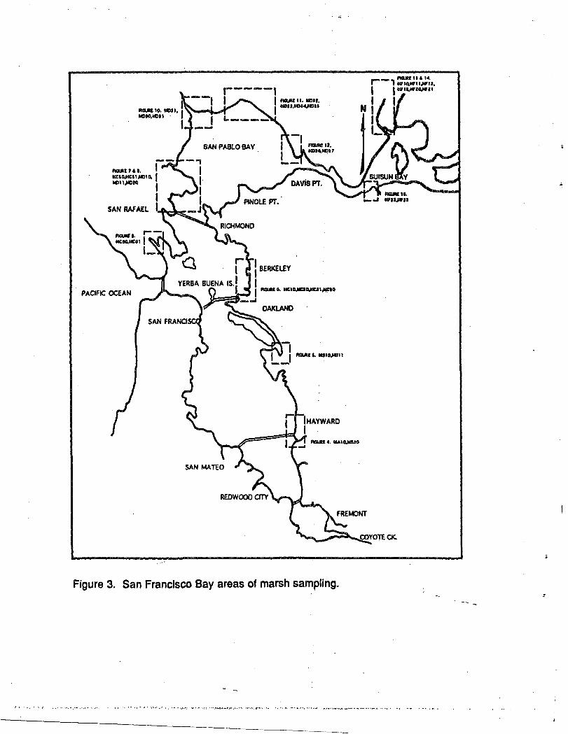
,-, ::.'.;:~~~r., , Wl....ro.wll

N I I1,-

IBERJ(£LEY

IflllId .. IIC'O.-:a~'~olb=~5:_~...

r----,I I IlUI II. IIDII.

",_........ I UllII.ICII~1I

--fIlIJlUU. ItIC'o.-:l1 ,/Cll0. I1ID11,l11lto I

ISAN RAFAEL I~~

PACIFIC OCEAN

Figure 3. San Francisco Bay areas of marsh sampling.

>•• ," .:.: •• ,,. •••••• •• ". ,~.,~,-•. ··'·· ..···.··.. ·v,· ' ·,.··.:: " ~" "',•• , , ",:-".-, ' ,:', ;, •.•••" ••.. ' .. ,_.~'"' 'f, _ - ~, , .- "" .- _

Figure 4 Gradient stations locations collected on May 25-27, 1991 with divercores.

SAN PABLO

- NORTH RICHMOND N

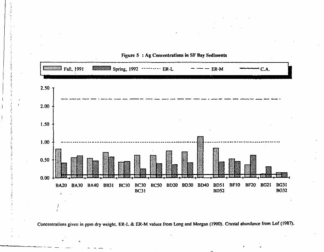
.,}·r

Figure 5 : Ag Concentrations in SF Bay Sediments

1'l1.;m.:<.Ei;;.<.E:E].Fa1.1'1i}.99.1••~.~•••sp.n•.n.g.'.19.9.2.-.-.--.-.--.-•.•E.R.-L•••••••E.R.-M•••~~~~~~.c•.A•.•••I2.50

2.00

1.50

,"

1.00

0.50

0.00

_.. --- --. --_ -_ -._-_ .. -_ .. --- ------ ---- ---------- _ -'---

BA20 BA30 BA40 BB31 BCto Be30 BC50 B020 B030 B040 B051 BFIO BF20 B021 B031BC31 BD52 B032

Concentrations given in ppm dry weight. ER-L & ER-M values from Long and Morgan (1990). Crustal abundance from Lof (1987).

".- ..

Figure 6 : Cd Concentrations in SF Bay Sedimell1lts

I 0

~ Spring, 1992 __ u u ER-L

'!. '(;,0" •

- -- ER-M ===C.A.

9.00 ----- ._--- --- -- --- -- ------ -------.

8.00

7.00

6.00

5.00 •. ............. -- .. -. - -- - coo .. _ -- - -- - .. -_ .. -- _ .. _ - .. -- -- .. _. _ .. _. - -_ -- .. -- _ --

4.00

3.00

2.00

1.00

0.00 J-c~::p5ii:~~~~~~~~=smep~!E!Cf~~~~

BA20 BA30 BA40 8B31 BCtO BC30 BC50 B020 B030 B040 BD51 BFtO BF20 B021 B031BC31 B052 B032

Concentrations given in ppm dry weight. ER-L & ER-M values from Long and Morgan (1990). Crustal abundance from Lof (1987).

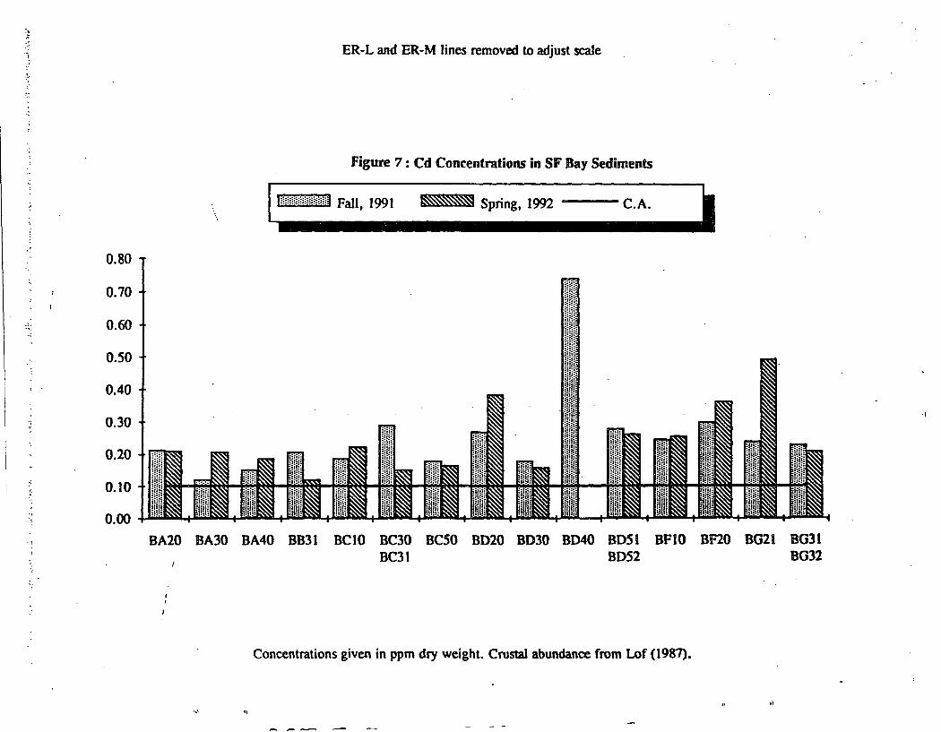
0.80

0.70

0.60

0.50

0.40

0.30

0.20

0.10

0.00

ER-L and ER-M lines removed to adjust scale

Figure 7 : Cd Concentrations in SF Bay Sediments

IUmi@ilii"@ Fall, 1991 ~ Spring, 1992 C.A. I­~---------------_I

BA20 BA30 BA40 BB31 BC10 BC30 BCSO B020 B030 B040 BOSIBC31 BD52

BPIO BF20 BG2l RG3l8032

Concentrations given in ppm dry weight. Crustal abundance from Lof (1987).

,...,.. ...... - -

Figure 8 : Cr Concentratiol/lS film SF Bay Sediments

HHW:m:~:HWI Fall, 1991 ~ Spring, 1992 n __ ER-L - -- ER-M =====C.A.

200

180

160

140

120

100

80

60

40

20

oBA20 BA30 BA40 BB31 BCIO BC30

BC31BC50 B020 B030 B040 B051

B052BFI0 BF20 B021 8031

8032

Concentrations given in ppm dry weight. ER-L & ER-M values from Long and Morgan (1990). Crustal abundance from Lof (1987).

,.-;"

Figure 9 : Cu Concentrations in SF Bay Sediments

1""'"m''''''',111 Fall, 1;91 ~ Spring, 1992 -_ ••• -- •• ER·L - - - ER-M --- C.A. ~_..._.... ...1350

300

250

200

ISO

100

50

o

!Ilili

BA20 BA30 BA40 BB31 DCtO BC30 DC50 B020 B030 D040 BOSI BFIO DF20 D021 B031BC3 t B052 B032

Concentrations given in ppm dry weight. ER-L & ER-M values from Long and Morgan (1990). Crustal abundance from Lof (1987)•

'f "•1

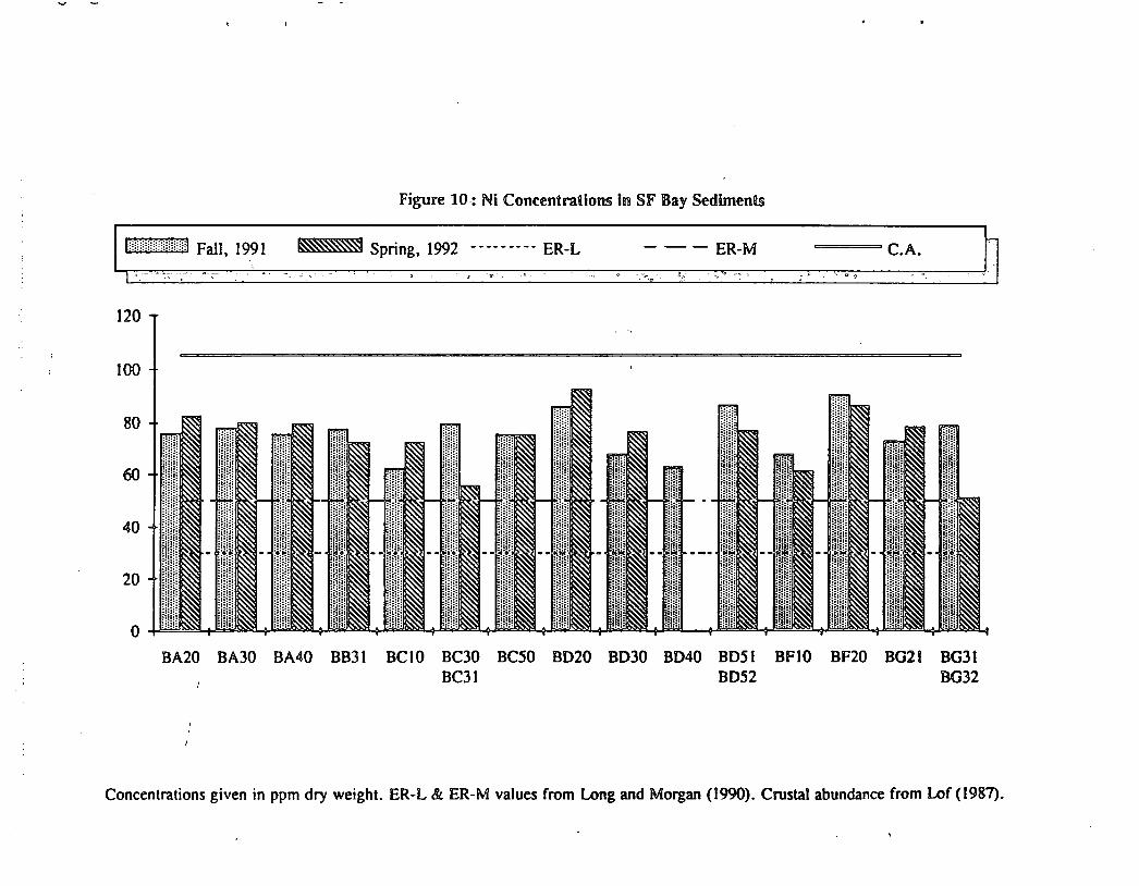
figure 10: Ni Concentrations in SJF Bay Sedimenis

HuHl'tmd Fall 1991 ~ Spring, 1992.,....

ER-L - -- ER-M--------- C.A.,

I' '" ',' " ,""

~"""':. <..;-~ " go

120

100

80

60

40

20

0

BA20 BA30 BA40 BB31 BCI0 BC30 BC50 B020 B030 B040 B051 BFIO BF20 BG2l DG3lBC31 B052 BG32

Concentrations given in ppm dry weight. ER-L & ER-M values from Long and Morgan (1990). Crustal abundance from Lof (1987).

Figure 11: Pb Concentrations in SF Bay Sediments

~ Spring, 1992 ~-------. ER-L - -- ER-M C.A. J120

100

80

60

40

20

o

- -- - - --- - - --- - - - - -- ---.-- - - -- - - _.

BA20 BA30 BA40 DB31 BCtO BC30 Be50 BD20 BD30 BD40 BD51 BFI0 BF20 BG21 B031BC31 BD52 B032

Concentrations given in ppm dry weight. ER-L & ER-M values from Long and Morgan (1990). Crustal abundance from Lor (1987).

.,'"

Figure 12: Zn Concentrations in SF Bay Sediments

300

250

200

150

- -- ER-M ====C.A.

100

50

oBA20 BA30 BA40 BB31 BCtO BC30 BC50 B020 8030 8040 8051 BFIO 8F20 8021

8C31 B052B031B032

Concentrations given in ppm dry weight. ER-L & ER-M values from Long and Morgan (1990). Crustal abundance from Lof (1987).

Figure 13: Ag Concentrations in Bay Area Creeks Bnd Marshes

1....'I@i•.i:1:ln::lml.nH.ml~I~.~cl:.:n.t~.tlio.n.-I-I--.-I-.-.-·.EIRI-IL••••::.IE.RI-.M•••:::~~~.CI·.AI·•••1.:~ 2.50

2.00

1.50

1.00 .

~I.,!j'\

..,.

MMMMMMMMMMMMMMMMMMMMMMMMMMMMMMMMRRRRRRRA B B Bee C C C C C C D D D D DD D D D D D D F F F F F F F F S S S S S S S111212235566112233333333111122221211111o 0,1 0 0 0 1 0 0 1 0 1 0 1 0 1 0 1 2 3 4 5 6 7 0 1 2 3 0 1 2 3 0 0 1 I I I I

Concentrations .given in ppm dry wei~ht. ER-L & ER-M values from Long and Morgan (1990). Crustal abundance from Lor (1987)•

• j

Figure 14: Cd Concentrations in Bay Area Creeks al1ld Marnlhles

mm!immmnA Sediment - - -- - -- _. ER-LConcentration

- -- ER-M ===·C.A.

(19.5)

10.00 111

9.00

8.00

7.00

6.00S 00 •• - - -- - _. - -- - _. - •• - - - _. - -. - - • -- - _. - .- - _•• _. - -- - -- • - - - - -- - _••••• -- - -- • - - -- - - • - - - - .: - - - -- - -- - -- - - - - - .- - -

;:: :11:,1

2.00 ~Il

1.00 .... ill0.00 .F:~~~¥:i£~~~~~~~~~~~~~~~~¥'~-':f!i'-"~"="-~'--~":;;::-'¢~~~~~-~~-~~-~

MMMMMMMMMMMMMMMMMMMMMMMMMMMMMMMMRRRRRRRA B B B C C C C C C C C D D D D D D D D D D D D F F F F F F P F S S S S S S S1 1 1 2 122 3 5 5 661 122 3 3 3 3 3 3 331 1 1 1 222 2 1 2 1 1 1 1 1o 0/1 000 1 0 0 1 0 1 0 1 0 1 0 1 2 345 670 1 230 1 2 300 1 1 1 1 1

Concentrations given in ppm dry weight. ER-L & ER-M values from Long and Morgan (1990). Crustal abundance from Lof (1987).

i:..l.II;";.,.,

I·

-- -

ER-L and ER-M lines removed to adjust scale

Figure 15: Cd Concentrations in Bay Area Creeks and Marshes

11i"'~i"i'*j Sediment Concentl1ltion ---C.A. ~......--- 1(19.5)

I.80 m rl~I'I',1.60 t"

::: I.,1&~ I:O·.·~200!1 i:;..:'..:;,I••:;•.:. ~..,.:'.•:""""':'. r,1i:i.l,~ l:;::.:~,:!.~,; r.!'•••:i.; :Ii,: ~,1,:..:1..:: _.,. _ , :.: :: ;;T'":.:••••,:••••':••••' •••••'; •••••••,1:.•••,; 1m Ii

""1 _ ~ ~ m mrH~HTI~ ~ ;II! 1ill: m 'It ~ mm1: mm

MMMMMMMMMMMMMMMMMMMMMMMMMMMMMMMMRRRRRRRABBBCCCCCCCCDDDDDDDDDDDDFFFFFFFFSSSSSSSJ J J 2 J 2 2 3 5 5 6 6 J J 2 2 3 3 3 3 3 3 3 3· J J I J 2 2 2 2 J 2 I 1 I I Io 0, ] 0 0 0 1 0 0 1 0 J 0 1 0 J 0 12 3 4 5 6 7 0 I 2 3 0 I 2 3 0 0 J I I 1

Concentrations given in ppm dry weight. Crustal abundance from Lof (1987).

Figure 16: Cr Concentrntions in Bay A.rea Creeks aJlluli MalfSiBes

11@@@mmnm Sediment - - -'" - -- _. ER-LConcentration

- -- ER-M ==='C.A.

I : ,- -, "'~ ~. ~" ,.., 0

200

180

160 .

140

:: . ~._._._-- ~ - ""'!I.~~'1f"-.; ••'.'.~ ._.~ ~ illt: ~ m ill 00 In mn ·:~,;.,:,:I.·::i:!::.: P.i!i:: ..!:..,..:.I:.:=•••,1-~..,:; :!::..,:~::: - rn!•.•••••.•••••:i:i•.....,~: .•••...:~·,!:;:' :!:..' :~!::;!:.:::,: . :;!, :!:: ;~!, l~ m ~~ mI j ~ !U Ji i ~ill ~ * ~ :.:: ,l ••••••••.•.•,l:,: :,1 :;.:: .••.....::: :::~ :·,1 :•..:~ ..:,1 ,j ::1::~ ,·:1 ::1 :·:1 ~ * * * * * ~ ~ ~ ¥ • f ~20 II! III III 1111 III I!I III I! III ~Il ;llilli !II~ ;l!~ ;II~ 111o~~~~~~~~~~~~~~~~~~~~~~~~~~~~~~~~~~~~

MMMMMMMMMMMMMMMMMMMMMMMMMMMMMMMMRRRRRRRA B B B C C C C C C C C D D D D D D D D D D D D F F F F F F F F S S S S S S S1 112 1 223 5 5 661 122 3 3 3 3 333 3 1 1 1 1 2 2 2 2 121 1 1 1 1o 0/1 000 1 0 0 1 0 1 0 1 0 lOt 2 3 4 5 670 t 230 1 2 3 0 0 1 1 I 1 I

Concentrations given in ppm dry weight. ER-L & ER-M values from Long and Morgan (1990). Crustal abundance from Lof (1937).

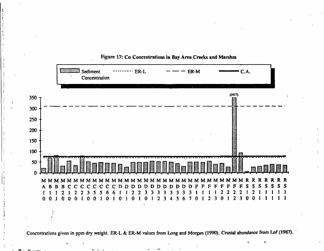
Figure 17: Cu Concentrations in Bay Area Creeks and Marshes

IMW~ti;;i'il ~~~=:"tion .--- ..--. ER·L - - -'- ER·M --- C.A. •________________I(29S7)

_________________________Itll

r:

1.1...\. ::

MMMMMMMMMMMMMMMMMMMMMMMMMMMMMMMMRRRRRRRABBBCCCCCCCCDDDDDDDDDDDDFFFFFFFFSSSSSSSI 1 121 2 2 3 S S 661 1 2 2 3 3 3 3 3 333 1 1 1 122 2 2 121 1 III00) 000 100 101 0 1 0 1 0 1 234 S 6 7 0 1 230 1 2 3 001 1 I 1 I

Concentrations given in ppm dry weight. ER-L & ER-M values from Long and Morgan (1990). Crustal abundance from Lof (1987).

,...,

ER-M tine removed to adjust scale

Figure 18: Cu Concentrrations un l!Jmy Arem C~ks amll MImll'§hes

--------- ER-L• . ".::U;::;L-.,,,,.~ '.,

~ , "'r '.,:,~.".

====C.A.-, -"0-''7-'''-'''--'"'' •

- - ',!"";i' .•

(29S7)

I,::f:..:~~' ~III

100

90

80

70

60­

50

40

30 .

20

10

o

--;; !:~ --- --- --- -~"." ....

I

-_. -- --- --- --- --- --- -- --- - -- --- --- --- ---- --- --- --- -_.. ----- -- -- - =ll

I I ~~

~! III IITo!ill; m II!;IH '11

il; *'.,

iU' Eii:''! m HI

I.::

II!:1' ::1

iii! III II:_:It Eill :li. Ell: Iii! I': ll! III!Ii! hH !H: HI H: iii: .., ~:2: :.:: i'i! ;H 0.:

iii! !"!' F.:!'i

"" ill ."i:l

l! ~!l~ ;m

""'! ;i;'~".!:' !lr!.l ...:II••:i••I...:l,..:1 ~•••••:',•••,;.'",:!,::,:"mIl! .:. 111iii :1' ll'l ill :~ I Iill hI j.1 'il :. .\:,.' :11'II' ii: .11 i:! ill.III Vi!iI l:: :11 ·n i I . r :li.

MMMMMMMMMMMMMMMMMMMMMMMMMMMMMMMMRRRRRRRA B 8 Bee C C C C C C D D D D D D DOD D D D F F F F f F F F S S S S S S S1 112 122 355 661 122 3 3 3 3 3 3 331 1 1 122 2 2 121 1 111001000100101010101234567012301230011111

Concentrations given in ppm dry weight. ER-L & ER-M values from Long and Morgan (1990). Crustal abundance from Lof (1987).

160

140

120

Figure 19: Ni Concentrations in Bay Area Creeks and Marshes

11;~'i,ti');'j"@ ~:~:"tion .._m__ • ER-L - - - ER-M ---C.A. I~........--........--........--I

""!'

t ~ 1!' .~:.::i::!.::::.:~:~II~ JI; .II: II

im

IIIil~ iH

"1W. ~~

III I

.'

MMMMMMMMMMMMMMMMMMMMMMMMMMMMMMMMRRRRRRRABBBCCCCCCCCDDDDDDDDDDDDFFFFFFFFSSSSSSS1 1 121 223 5 5 661 122 3 3 3 3 333 3 1 J J 122 2 2 121 111 100100 0 100 1 0 1 0 1 0 101 2 345 670 I 230 I 2 3 001 111 I

I

Concentrations given in ppm dry weight. ER-L & ER-M values from Long and Morgan (1990). Crustal abundance from Lor (1987).

."

1" i"

, .I. :.,

i !!

Figure 20: I?b Concentrations Dn Bay Area Creeks mruB Mmll"§ll1es

- - - ER-M C.A.

II! - - - - - ~----- - - - - -- -- -----.

I~:~:w@:m:~mml Sediment - - -- - -- _. ER-L

Concentration

50

100

150

200

250

MMMMMMMMMMMMMMMMMMMMMMMMMMMMMMMMRRRRRRRA B B B C C C C C C C C D D D D D DOD D D D D F F F F F F F F S S S S S S SI 112 1 223 5 5 661 122 3 3 3 3 3 333 1 I I 122 2 2 121 I 1 I Io 0, 1 0 0 0 1 0 0 I 0 I 0 I 0 I 0 I 2 3 4 5 6 7 0 I 2 3 0 I 2 3 0 0 I I I I I

Concentrations given in ppm dry weight. ER-L & ER-M values from Long and Morgan (1990). Crustal abundance from l.::of (l9~1).

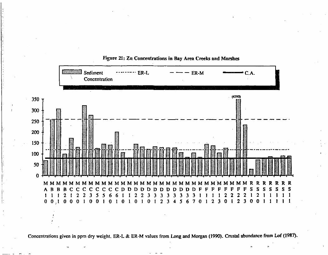
·, Figure 21: Zn Concentrations in Bay Area Creeks and Marshes

1,;,m'I!~'fml ~~::~tion -..-----, ER-L - - - ER-M ---C.A. I_---------------I350

300

250

200

150

100 ~

m

II ,·,~"""":;":~,,,,,,:i:::!.i.JIII

1- ~...:l..:..~...:~:.:: _f:lli1..:~.:.:;..:~...:: - ~.r.:...:!;...:! -;....:...:...: - - ~ ;;; ~ -~- '1_ ~!II !!I iii !!I ill !II

. (4390)

------_.

", ]i- m>---'-f------------:.-

I ~ I ~~~ II ~I II I :1 IiIIJ~ ~1 i~ IIII :11 i .f: 'II. j' i JHe

Ii; :II .m ~i:

MMMMMMMMMMMMMMMMMMMMMMMMMMMMMMMMRRRRRRRA B B B C C C C C C C C D D D DOD D DOD D D F F F F F F F F S S S S S S SI I 121 2 2 3 5 5 661 122 3 3 3 3 3 333 I 1 I 122 2 2 121 1 I I Io 0,10 0 0 100 I 010 1010 12 3 4 5 670 I 230 12 300 I 1 I I 1

Concentrations given in ppm dry weight. ER-L & ER-M values from Long and Morgan (1990). Crustal abundance from Lof (1981).

'f! .. ..

Figure 20: Ph COr1lcentntions in 13m)' Ares Cuwks mllUlI Mmrrslhles

mmm~@@mmi Sediment --------. ER-LConcentration

- -- ER-M 'd'le.A.

250

200

150!II

m100

m

50

0

III_________________ .-:::=a _

MMMMMMMMMMMMMMMMMMMMMMMMMMMMMMMMRRRRRRRA B B Bee C C C C C C D D D D D D D D D D D D F F F F F F F F S S S S S S S1 112 122 3 5 5 661 122 3 3 3 3 3 3 3 3 1 1 1 122 2 2 121 1 ttlo 0 /1 0 0 0 1 0 0 1 0 1 0 1 0 1 0 I 2 3 4 5 6 7 0 I 2 3 0 1 2 3 0 0 1 til 1

Concentrations given in ppm dry weight. ER-L & ER-M values from Long and Morgan (1990). Crustal abundance from lof (19~7).

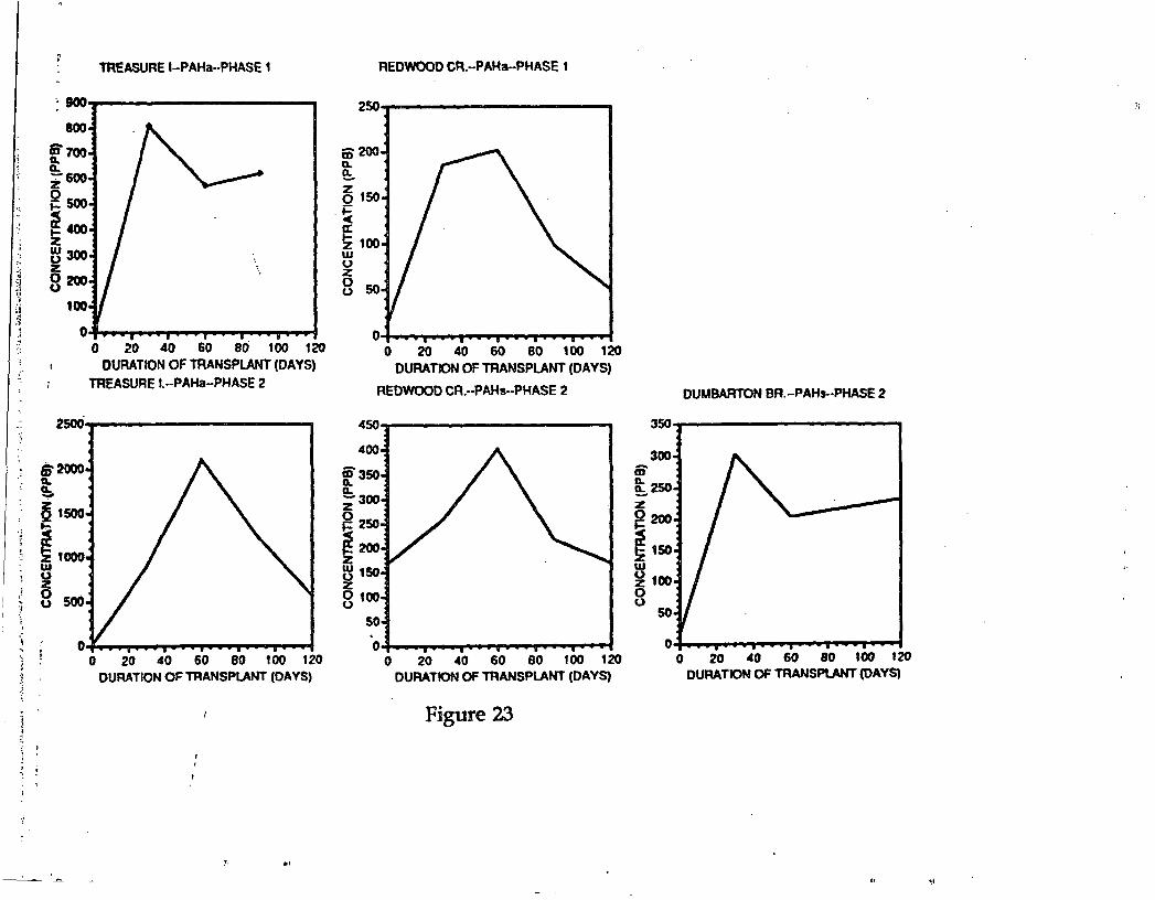
TREASURE I-PAHa··PHASE 1 REDWOOD CR.··PAHa--PHASE 1

: 900....---------..

800

tD'7000..0..

i 600

~SOO

~Coo~300z8 200

100

O.......,,.......-ro.......,.......,,.......,.-..oo4o 20 40 60 80 100 120

DURATION OF TRANSPlANT (DAYS)TREASURE 1.-·PAHa-PHASE 2

250.....----------_

ii)2000..~

~150.~a:!z 100wUz8 50

O~-.....-.._,..,,..........- ............o 20 40 60 80 100 120

DURATION OF TRANSPLANT (DAYS)

REDWOOD CR.--PAHs-PHASE 2 DUUBAATON BR.-PAHs--PHASE 2

50

O.._ ............- ....-..-..,,.--io 20 .0 60 80 100 120

DURATION OF TRANSPLANT (DAYS)

350_----------...

.0+._....._.._,..,,..........- ......- ...

o 20 40 60 80 100 120DURATION OF TRANSPLANT (DAYS)

450_------------.400

m3500..0..z300

°250~200~150z0100u

SO

2500'.....---------......

Oof.-....,,......-yo-'T'P~,....._r.....pofo 20 40 60 80 100 120

DURATION OF TRANSPlANT (DAYS)

fj20000..~

~1500

',: ~ 1000

w

~u 500

Figure 23

.," a'

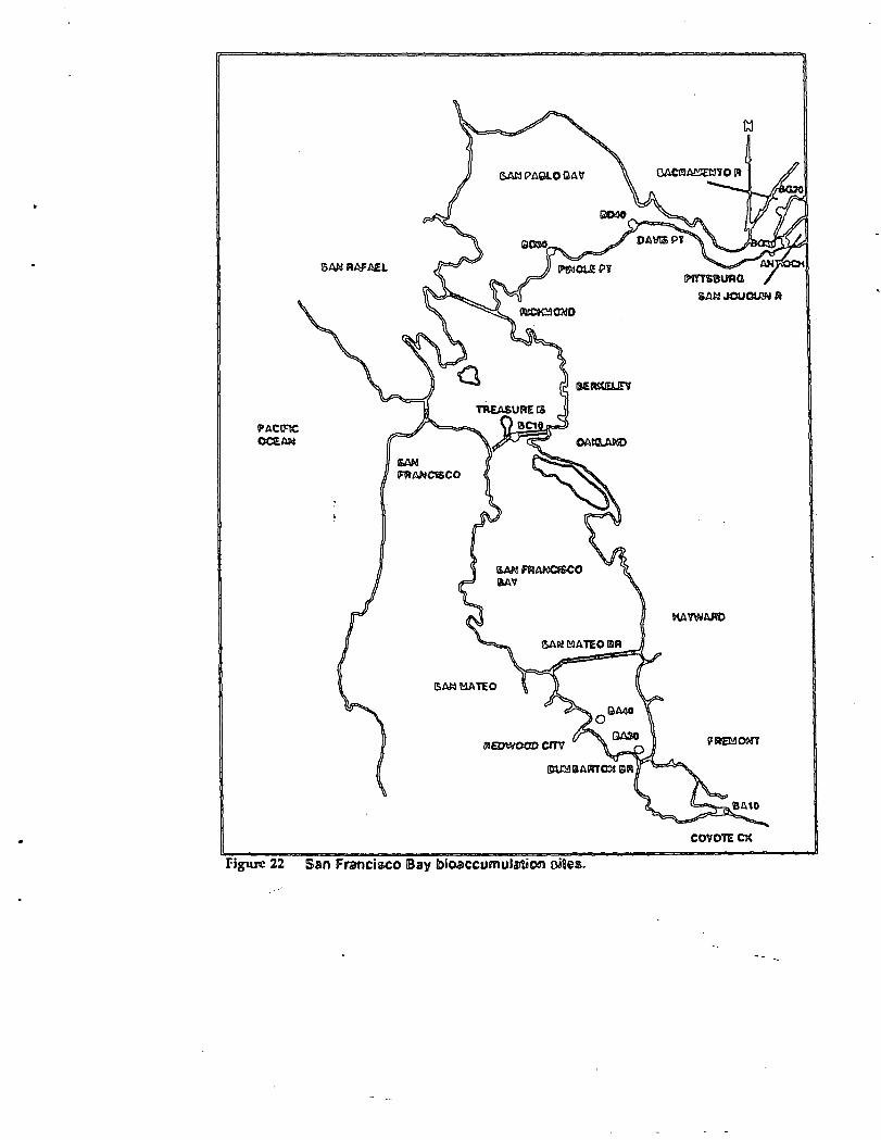
5A1\l RAfAEL

5Ml~ATEO

covon CK

Figure 22 San fr.mci~o Bay loioaccumul&rt.ioo o.ite$.

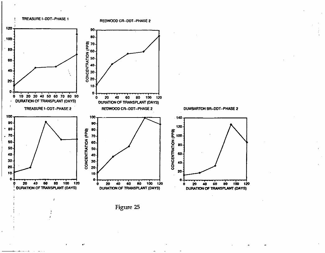
TREASURE I-DDT··PHASE 1 REDWOOD CR··DDT··PHASE 2

100

80.

DUMBARTON BR-DDT-PHASE 2

90.....------------.

80

m700.0.;-60

Q so~~ 40

~ 30z8 20

10

O-l-o-......or_......,r"""""'......,-......,........"""'T"_~o 20 40 60 80 100 120

DURATION OF TRANSPlANT (DAYS)

REDWOOD CR-·DDT-PHASE 2

40

20

O-f-__- .........,.....-.-....,........,.......~o 10 20 30 40 50 60 70 80 90

I DURATION OF TRANSPLANT (DAYS)

TREASURE I-DOT-PHASE 2

120,,1 ...,.

60

100_-----------,

·00

• 80

• 70

60

50

40

30

20

10

O....-~-or_......,..__-~-_fo 20 40 60 80 100 1201DURATION OF TRANSPlANT (DAYS)I

1oo-r----------r----,90

iii 800.~ 70z 60

~ 50~ 40w~ 30

8 20

10O~ ..._........._-.....-r_--t

o 20 40 60 80 100 120DURATION OF TRANSPlANT (DAYS)

140""1""'""------------,

120iii~1oozQ 80~

~ 60w~ 40ou

20

O.J-...........-~__,-...,. .........,.-~o 20 40 60 80 100 120

DURATION OF TRANSPlANT (DAYS)

Figure 25

.' .,

..

TREASURE 1··PCBs-PHASE t

3!50CY============;J

so

o~~"iF""v=;;=~;;=v=;r=;=;;=;;"""",=v=;;=v=;;=~1

o 20 40 60 80 100 120DURATION OF TRANSPLANT (DAYS)

TREASURE I..PCB9-·PHASE 2

160-?-------------.

O+--~-T"""-.,__.......,.......-,......._fo 20 40 60 80 100 120

DURATION OF TRANSPLANT (DAYS)I

REDWOOD CR··PCBs-PHASE 1

300.,...------------.

_250co0.0.;;200o~15Oa:.­·z~100zoo 50

o{t.............,.............,__.......T"""""-,..............,I""""'",.....,fo 20 40 60 80 100 120

DURATION OF TRANSPLANT (DAYS)

REDWOOD CR.-PCB9-·PHASE 2

250 __------------,

o-f-t........."T'"'"......'T'"""'.......,.............,............,r-""-1o 20 40 60 80 100 120

DURATION OF TRANSPLANT (DAYS)

Figure 24

DUIVIJBARTO\\I BR.-P CBg-PHASE 2

200-y-----------.....,180

iD 160Q.

~140

a:: 120

~'COi 00au~ 60

8 40

20

0-f--"T'"'"-""'-""""-""""""""r""""""""1o 20 40 60 80 100 120

DURATION OF TRANSPLANT (DAYS)

TREASURE '·-eHLORDANE··PHASE t

t8....-----__~ _

t6

iii't4Q.Q.

Z12

~ 10c~ 8wCo)

~Co)

o 20 40 60 80 100 120DURATION OF TRANSPLANT (DAYS)

TREASURE I-eHLORDANE·-PHASE 2

25....---- _

620~

~ t5

~ 10wCo)

8 5

O~- ..... ...

o 20 40 60 80 100 120DURATION OF TRANSPlANT (DAYS)

..'

em- non

REDWOOD CR.·· CHlORDANE­PHASE t

30....---- -.

-.25mQ.Q.

Z20o~ t5~z~ 10zoo 5

O+-._....._...-~_ ..... ...

o 20 40 60 80 tOO 120DURATION OF TRANSPLANT (DAYS)

REDWOOD CR-CHLORDANE··PHAS2

30....---- _

-.25mQ.

e.. 20zQ~ 15

~~ tozou 5

0+. ..- ...

o 20 40 60 80 100 120DURATION OF TRANSPLANT (DAYS)

Figure 26

DUMBARTON BR.-CHLOROANE-PHASE 2

30....-------.....--..,.

O+.....,,...........-...,...-r-...,.-"1o 20 40 60 80 100 120

DURAT.ION OF mANSPLANT (DAYS)

".,

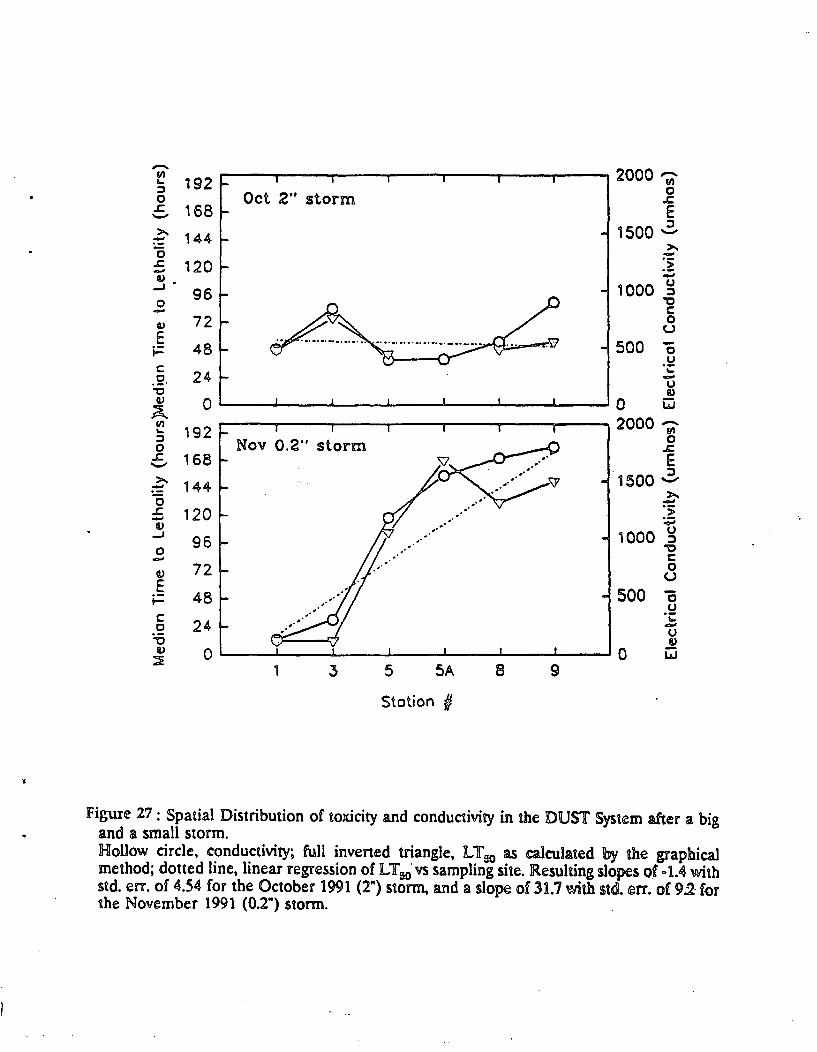
- 2000 Iii"III192~

:::J 00 .c

.J:: 168 E'-'"

1500 2->.. 144cJ

>..'0 cJ

.c 120 :~cJcJ

~.96 1000 g

0 -0C- 0CL) 72 u

E 500t= 48 0u

c ·C24 cJ.51. u

." tlJQ) 0 0 wA

2000 YlIII192~

0:::J0 .r..c 168 E'-'"

1500 2->.. 144-~ >.15 -.J:: 120.;;

cJ :;:;Ci)

1000 u-J96 :::l

0 -0CcJ

0Ci) 72 uE

48 500 "0t= uc .b:

24 ..:oJ0 0:.c flJILl 0 0 w~

Station II

Figure 27 : Spatial Distribution of toxicity and conductivity in the DUST System after a bigand a small storm.Hollow circle, conductivity; full inverted triangle, lLTso IS calculated by die graphicalmethod; dotted line, linear regression of lLTso' vs sampling site. Resulting ~lopes Qf D 1.~ withstd. err. of 4.54 for the October 1991 (2") storm, and a slope of 31.7 with std. err. of 9.2· f-orthe November 1991 (0.2") storm.

-oo 40>.:;"'­::l

II)

~ 20

c:.2-ocE"'­Q)~-(/)Q)~

100

80

60

• I

O~----::E- --J- "'---J

2 5

Doy From Storm Onset

8

Figure 28: Survival of Ceriodaphnia in DUST System samples taken after the storm of March14, 1992.Five field-replicates in each station had S test animals each, with daily renewal and feeding.Survival in all control chambers was 100% at test termination, which was after 7 days exceptfor the test with March 15 samples.· Mean survival after 5-day exposure (Station 5, fulldiamonds) or 7-day exposure (Station 3, full circles) is presented.

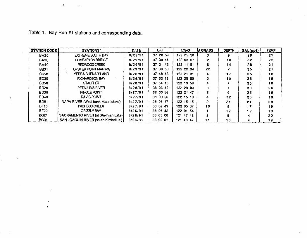
Table 1. Bay Run #1 stations and corresponding data.

STATION CODE STATIONS· DATE tAT LONG 11 GRABS DEP'rn SAL(ppt) TEMP8A20 EXTREME SOUTH BAY 8/29/91 37 28 59 122 05 28 3 9 28 238A30 DUMBARTON 8RIDGE 8/29/91 37 30 44 122 08 07 2 10 32 228MO REDWOOD CREEK 8/29/91 37 31 42 122 11 51 6 14 28 218B31 OYSTER POINT MARINA 8/29/91 37 39 50 122 22 34 20 7 35 218C10

"

VERBA BUENA ISLAND 8/28/91 37 48 46 122 21 31 17 35 184BC30 RICHARDSON BAY 8/28/91 37 52 16 122 29 50 2 10 38 188C50 STAUFFER 8/28/91 37 54 10 122 19 59 4 7 35 188020 PETALUMA RIVER 8/28/91 38 06 42 ' 122 29 00 3 7 30 208030 PINOlE POINT 8/27/91 38 00 56 122 21 47 8 9 25 188040 DAVIS POINT 8/27/91 38 03 20 122 15 10 4 12 25 198051 NAPA RIVER (West bank Mare Island) 8/27/91 38 05 17 122 15 15 2 21 21 20BF10 PACHECO CREEK 8/27/91 38 02 49 122 05 37 10 5 17 19BF20 GRIZZLY BAY 8/26/91 38 05 42 122 01 54 1 12 12 19BG21 SACRAMENTO RIVER (at Sherman Lake) 8/26/91 38 03 06 121 47 42 8 9 4 20BG31 SAN JOAQUIN RIVER (south Kimball Is.) 8/26/91 38 02 01 121 49 42 11 10 4 19

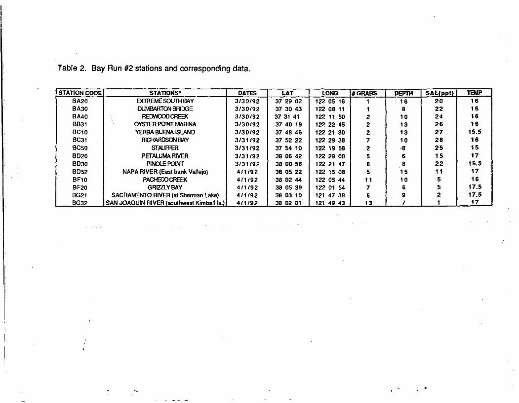
Table 2. Bay Run #2 stations and corresponding data.

STAnON CODE STAnONS· DATES LAT LONG # GRABS DEPTH SAl(ppt) TEMPBA20 EXTREME SOUTH BAY 3/30/92 37 29 02 122 05 16 1 16 20 16BA30 DUMBARTON BRIDGE 3/30/92 37 30 43 122 08 11 1 8 22 16BA40 REIJM:X)[) CREEK 3/30/92 3731 41 122 11 50 2 10 24 16BB31 OYSTER POINT MARINA 3/30/92 37 40 19 122 22 45 2 13 26 16

BC10 VERBA BUENA ISlAND 3/30/92 37 48 46 122 21 30 2 13 27 15.5

BC31 RICHARDSOO BAY 3/31/92 37 52 22 122 29 38 7 10 28 16

BC50 STAUFFER 3/31/92 37 54 10 122 19 58 2 IS- 25 15

B020 PETALUMA RIVER 3/31/92 38 0642 122 29 00 ·5 6 15 17B030 PINOlE POINT 3/31/92 38 00 56 122 21 47 8 8 22 16.5

B052 NAPA RIVER (East bank Vallejo) 4/1/92 38 05 22 122 15 08 5 15 11 17BF10 PACHECOCREE< 4/1/92 38 02 44 122 05 44 11 10 5 16

BF20 GRIZZl..Y BAY 4/1/92 38 05 39 122 01 54 7 6 5 17.5BG21 SACRAMENTO RIVER (at Sherman Lake) 4/1/92 38 03 10 121 47 38 6 9 2 17.5BG32 SAN JOAOUIN RIVER (southwest Kimball Is.) 4/1/92 38 02 01 121 49 43 13 7 1 17

'<., .1

.Table 3. Marsh stations and corresponding data.

STAllON coce STAllONS DAle SAlKllrTV (DDt) TYPE m: COUECTlONMA10 COYOTE HIlLS SLOUGH 11/25/91 19 TlSES11.4910 SAN LEANDRO BAY/ARAOYoIHEAD MARSH 11/25/91 30 T\JBESMB11 SAN LEANDRO BAYIGARRETSON POINT 11/25/91 30 l'\JBESMB20 SANLOOBllZOCREB< 11/25/91 34 TlSESMC10 RDlMONO INNER HARBORtlOFFMAN MARSH 11/26/91 30 TUBESMC20 CEAArTOCREB<MOl1Ili 11/26/91 32 TUBESMC21 ClOflOORNX::E5 CREB< MOUTH 11/26/91 30 TlSESMC30 EMERYVIU.E MARSH1:BMUD SToo.4DRAIN 2/21/92 28 NONalIER SCRAPEMC50 CORTE MADERA MARSH S. OF INDUSTRIAl. ROAD 2/17/92 28 NCRII-OlVER SCRAPEMC51 comE MADERA CREB<.lAAI<SPUR FERRY MARSH 2/17/92 27 NQ'o&.DlVER SCRAPEMC60 SILVA ISLAND MARSl-WEHIND CHEVRON 2118/92 27 NCm:)lI,IER SCRAPEMeGl SILVA ISLAND MARSWSEMINAR DR. STORMDRAIN 2/18/92 28 NO'HlIVER SCRAPE11.4010 MILLER CREEKAAS GALllNAS DISCHARGE 2/19/92 27 NON-OOIER SCRAPE11.4011 MllERCREEKAJPSTREAM FROM OISO-fARGE 2/19/92 28 NON-OIVER SCRAPE11.4020 GALLINAS CREEKOOHN F. McINNIS COUNTY PARK 2/19/92 28 NGH)lVER SCRAPEMD21 NOVATOCREEKIATLOCK 2/19/92 28 NQN.DlVERSCRAPE11.4030 PETALUMA RIVER MO\JTHIE. BANK MARSH 11/1/91 27 lllBESMD31 TOLAY CREEK MOUTH 11/1/91 26 lUBESMD32 NAPA SLOI.IGI-WRIDGE 11/1/91 26 TUBES11.4033 SONOMA CREEK1TUB8S 11/1/91 26 TI.J8ES11.4034 SONOMA~RJDGE 11/1/91 26 TI.J8ES1'.4035 INLET EAST OF NAPA SLOUGH 10/31/91 25 TI.J8ES1'.4036 MARE ISLAND NORll-IEA'l TIP 10/31191 23 ruses11.4037 MARE ISLAND CENTRALIAT PILES 10/31191 25 TlSESMF10 BOYNTON SLOUGH C1 7/23/91 20 OlVER SCRAPEMF11 BOYNTON SLOUGH C3 7/23/91 20 OlVER SCRAPEMF12 BOYNTON SLOUGH C4 7/23/91 20 OIlIER SCRAPEMF13 BOYNTON SLOUGH CR2 7/23/91 20 OIlIER SCRAPEMF20 HILL SLOUGWSaOW BRIDGE 7/24/91 20 OlVER SCRAPEMF21 HILL SLOUGH/ABOVE BRIDGE 7/24/91 21 OIlIER SCRAPEMF22 PEYTON SLOI..JGWAO< END OF SLOUGH 7/24/91 20 OIlIER SCRAPEMF23 PEYTON SLOI.JGK'MOUTl-l OF SLOUGH 7/24/91 21 OIlIER SCRAPEASl0 TOMALES BAY/ BRAZIL BEACH . 29 OIlIER SCRAPEASll TOMALES BAY/ MARCONI COVE .. 22 0lIIER SCRAPERS20 lAKE MENClCClNO ... 20 DIVER SCRAPE

4/8/91,7/16/919/3/91,10/31/91,11/26/91,2/21/92,4/2/92

4/24/91,6110/91,7/16/91,9/16/91

Table 4 Statistical Summary of Trace Element Concentrations in San Francisco Bay Sediments

Fall, 1991 (Dry Weather); n=15

Mean SD Median Max Min

Cr 76 8 78 87 61

Zn 112 16 111 137 77

Co 16 2 16 19 14

Ni 76 8 76 90 62

V 61 6 63 73 50

Cu 45 24 39 124 22

Cd 0.25 0.14 0.23 0.74 0.12

Ph .39 24 36 110 8

Ag 0.60 0.27 0.63 1.16 0.10

Spring, 1992 (Wet Weather) n= 14

Mean SD Median Max Min

Cr 79 12 83 92 47

Zn 109 17 115 127 73

Co 16 2 16 20 II

Ni 74 II.

77 92 51

V 61 9 62 81 41

Cu 41 8 . 40 S4 24

Cd 0.24 0.10 0.21 0.49 0.12

Ph 29 II 29 S6 9Ag 0.42 0.14 0.43 0.63 0.13

Values Reported in mg analyte per kg dry sediment (ppm)

<

Table 5 Bay Sediment Toxicity Tests - EohaustoriusMean survival ± SD of Eohaustorius estuarius in bay test sediments. "Home" (H)treattnents. and reference sediments (RS 11). Significant differences between survival intest sediments and "home" and reference tretments is indicated (ANOVA Fisher multiplerange test of arcsin(x) transfonned % survival values, p,O.OI). n= 5 replicates. with 20 or16 individuals/replicate.

Test Date StationSDaniftt8lDft Jl)ill1~(l~

Mean ±SD IRS lHl19/20/91 RS 11 17 2n=20 H 19 1

BA20 9 2 X XBA30 10 3 X XBA40 10 2 X XBB 31 14 2 X XBC 10 19 1BC30 10 4 X XBC50 17 . 1 XBD20 12 3 X XBD30 15 4 XBD40 18 1BD51 11 2 X XBF 10 14 2 X XBF20 13 2 X XBG21 17 2BG 31 19 0

4/15/92 RS 11 10 2n=16 H 14 1

BA20 7 2 XBA30 8 3 XBA40 10 0 XBB 31 10 2 XBC 10 11 1 XBe31 9 5 XBC50 8 1 XBD20 9 2 XBD30 14 2 XBD52 9 3 XBF 10 11 1 XBF20 8 3 XBG 21 9 3 XBG32 14 2 X

5-35

Table 6 Bay Sediment Toxicity Tests - Rhepoxinius .Mean survival ±SD ofRhepox;n;us abronius in bay test sediments,"Home" (H)treattnent, and reference sediment (RS 11). Significant differences between survival intest sediments and "Home" and reference treatments are indicated (ANOVA Fishermultiple range test of arcsin(x) transfonned % survival values, p<O.OI). n= 5 replicates.with 20 individualslreplicate.

Test Date StationSlpllicant Difference

Mean ±SD RS 11 H9/18,91 RS 11 19 1

H 20 1BA20 13 . 5 X XBA40 17 2BB3. 17 2BC30 14 2 XBC50 17 2BD40 16 ·4

Table 7 Bay Sediment Toxicity Tests - DaphniaMean survival ±SD and mean number of babies ±SO ofDaphnia magna in bay testsediments and reference sediment (RS 20). No significant difference between treatmentswas found (ANOVA Fisher multiple range test of arcsin(x) transformed % survivalvalues and number of babies. p<O.05). n= Sreplicates? with 10 individualslreplicate.

Test Date9/19191

StationRS 20BG21BG 31

. Mean±SDSurvival # of Babies

9 1 56 379· 1 70 379 1 55 41

-.

"'0,' " ~ , ,;. '.~" '_0: ..•••,. ·.r·. , " ' ' ~ ..•'_' ". '__ ' ;:. "~ __ ,

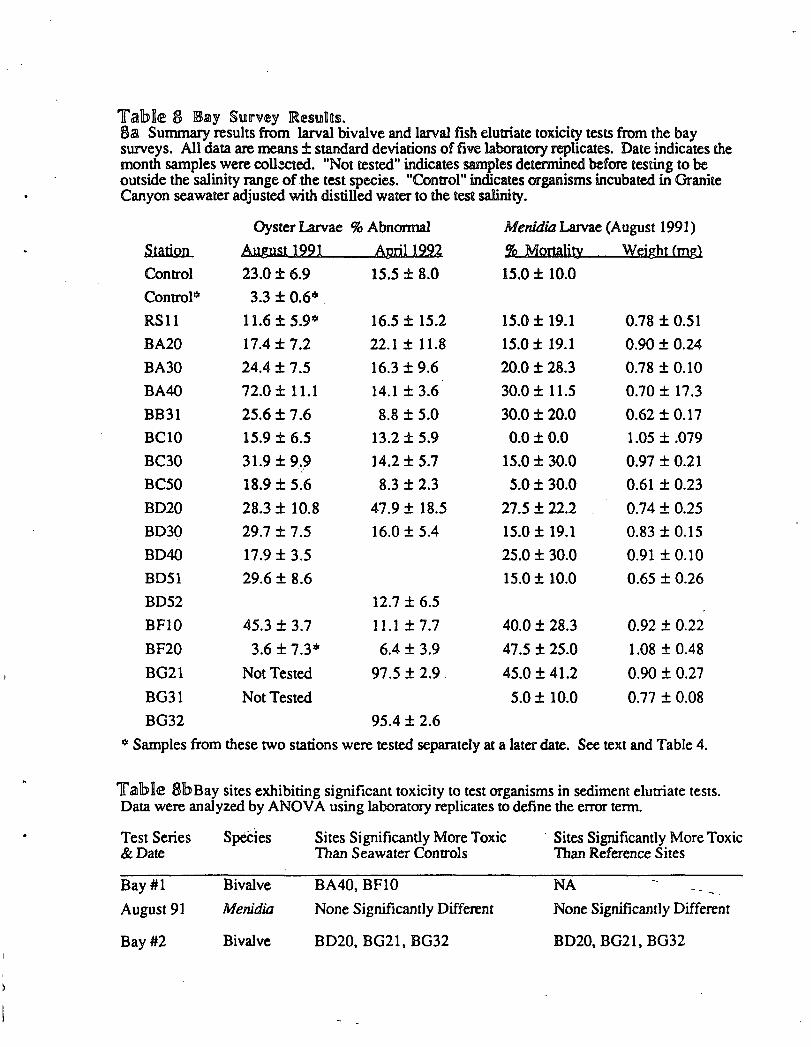
1fclll1blne 8 ~ay SUllIl"'V~Y IRes1llIUs.8:al Summary results from larval bivalve and larval fish elutriate toxicity tests from the baysurveys. All data are means ± standard deviations of five laboratory replicates. Date indicates themonth samples were coll:eted. "Not tested" indicates samples detennined btfore testing to beoutside the salinity range of the test species. "Control" indicates organisms incubated in GraniteCanyon seawater adjusted with distilled water to the tesi salinity.

Oyster Larvae % Abnonnal Menidia Larvae (August 1991)

Station AugYst 1991 A12riI1992 % Mortality Weight (mgl

Control 23.0 ± 6.9 15.5 ± 8.0 15.0 ± 10.0

Control'" 3.3 ± 0.6*

RSll 11.6 ± 5.9* 16.5 ± 15.2 15.0 ± 19.1 0.78 ± 0.51

BA20 17.4 ± 7.2 22.1 ± 11.8 15.0 ± 19.1 0.90 ± 0.24

BA30 24.4 ± 7.5 16.3 ± 9.6 20.0 ± 28.3 0.78 ± 0.10

BA40 72.0 ± 11.1 14.1 ± 3.6 30.0 ± 11.5 0.70 ± 17.3

BB31 25.6 ± 7.6 8.8 ± 5.0 30.0 ± 20.0 0.62 ± 0.17

BC10 15.9 ± 6.5 13.2 ± 5.9 0.0 ± 0.0 1.05 ± .079

BC30 31.9 ± 9.9 14.2 ± 5.7 15.0 ± 30.0 0.97 ± 0.21

BC50 18.9 ± 5.6 8.3 ± 2.3 5.0 ± 30.0 0.61 ± 0.23

BD20 28.3 ± 10.8 47.9 ± 18.5 27.5 ± 22.2 0.74 ± 0.25

BD30 29.7 ± 7.5 16.0 ± 5.4 15.0 ± 19.1 0.83 ± 0.15

BD40 17.9± 3.5 25.0 ± 30.0 0.91 ± 0.10

BD51 29.6 ± 8.6 15.0 ± 10.0 0.65 ± 0.26

BD52 12.7 ± 6.5

BFlO 45.3 ± 3.7 l1.l±7.7 40.0 ± 28.3 0.92 ± 0.22

BF20 3.6 ± 7.3* 6.4 ± 3.9 47.5 ± 25.0 1.08 ± 0.48

BG21 Not Tested 97.5 ± 2.9. 45.0 ± 41.2 0.90 ± 0.27

BG3l Not Tested 5.0 ± 10.0 0.77 ± 0.08

BG32 95.4 ± 2.6

* Samples from these two stations were tested separately at a later date. See text and Table 4.

1falblle 81blBay sites exhibiting significant toxicity to test organisms in sediment elutriate tests.Data were analyzed by ANOVA using laboratory replicates to define the error tenn.

Test Series Species Sites Significantly More Toxic . Sites Significantly More Toxic& Date Than Seawater Controls Than Reference Sites

Bay #1 Bivalve BA40, BFlO NA

August 91 Menidia None Significantly Different None Significantly Different

Bay #2 Bivalve BD20, BG2l, BG32 BD20, BG2l, BG32

5-36

Table 9 Marsh Toxicity Tests· EohtJuStoriusMean survival ±SO of Eohaustorius estuarius in marsh test sediments. "Home" (H)treattnents, and reference sediment (RS 10 or RS 11). Significant differences betweensurvival in test sediments and "Home" and reference trearments me indicated forsignificance levels listed (ANOVA Fisher multiple range test of arcsin(x) transformed %survival values). n=5 replicates. with 20 individuals/replicate in all tests except 7/26/91,in which there were 12 individuals!replicate.

H 10 ~MFI0 4 1 XMFll 5 2· XMF12 5 2 XMF13 8 3 XMF20 6 2 XMF21 5 3 XMF22 6 3 XMF23 8 1 X

p=O.05 H 1MD30 3 XMD31 3 X XMD32 2 X XMD33 2 X XMD34 2 X XMD35 2 XMD36 3MD37 1 X

1p=O.OI· 2

32 X22221

p=O.05 H 18 1 :;;

MC30 11 5 XMCSO 12 3 X

#0'#

MC51 14 3 X XMC60 17 2 XMC61 . 16 2 X XMOIO 15 4 X XMOll 15 3 X XMD20 8 3 XM021 10 2 X

Table l~Msllrsllu SIlIJn'<ey lR<esIlIJDlts.1~aSummary results from larval bivalve and larval fish elutriate to,uclty aests from the marshsurveys. All data are means ± standard deviations of five laboratory replicanes. Date indicates themonth samples were collected. "No~ tested" indicates samples determined ~fore testing to beoutside the salinity range of the test species. "Control" indicates organisms incubated in GraniteCanyon seawater adjusted with distilled water to the test salinity.

Oyster Larvae Menidia Larvae Atherinops LarvaeDate Station % Abnounal % MortalitY WeightCmg) % Mortality Weight (rog)

July 91 Control 15.7 ± 10.0 7.5 ± 6.8 0.70 ± 0.08 0.0 ± 0.0 0.98 ± 0.12

lRSI0 74.8 ± 6.9 7.5 ± 11.2 0.75 ± 0.10 4.0 ± 8.9 1.15 ± 0.15

LM l00.0± 0.0 24.7 ± 12.9 0.72 ±0.13 28.0 ± 30.3 0.98 ±0.31

MFlO 94.6 ± 2.6 10.0 ± 10.5 0.80± 0.09 0.0 ± 0.0 1.16 ± 0.12

MF11 61.0 ± 6.9 5.0 ± 6.8· 0.73 ± 0.08 0.0 ± 0.0 1.11 ± 0.08

MF12 63.3 ± 13.9 10.4 ± 10.6 0.72 ± 0.07 4.0 ± 8.9 1.11 ± 0.10

MF13 73.4 ± 7.3 12.5 ± 12.5 0.82 ± 0.08 8.0 ± 17.9 1.09 ± 0.02

MF20 Not Tested 5.0 ± 6.8 0.76± 0.08 4.0 ± 8.9 0.97 ± 0.16

MF21 Not Tested 10.4 ± 10.6 0.68 ± 0.06 48.0 ± 26.8 1.14 ± 0.21

MF22 12.3 ± 6.6 5.0± 6.8 0.79 ± 0.07 0.0 ± 0.0 1.21 ± 0.12

MF23 39.9 ± 10.1 2.5 ± 5.6 0.69 ± 0.05 0.0 ± 0.0 1.14 ± 0.10

Oct. 91 Control 1.9 ± 1.7 8.0 ± 11.0 1.03 ± 0.19

REll 1.2 ± 1.1 4.0 ± 8.9 1.11 ± 1.24

MOJO 2.6 ± 2.0 O.O± 0.0 1.25 ± 0.17

MD31 1.4 ± 0.6 o.o± 0.0 1.28 ± 0.24

MD32 1.8 ± 1.2 4.0 ± 8.9 1.15 ± .26

M033 1.5 ± 1.4 8.0 ± 11.0 1.18 ± .28

MD34 0.4 ± 0.6 4.0 ± 8.9 1.69 ± .741

MD35 0.7 ± 0.6 O.O± 0.0 1.46 ±0.13

MD36 1.1 ± 0.7 O.O± 0.0 1.16 ± 0.29

MD37 1.2 ± 1.1 O.O± 0.0 1.15 ± 0.23

Oct. 91 OysterLaryae in Pore Water!

Control .- 4.7 ± 1.3

1RE11 10.7 ± 5.9 (n =2)

MD36 6.5 ± 4.2

MD37 4.5 ± 2.1

t Pore water =supernatant water remaining above settled sediment in original sample jars.

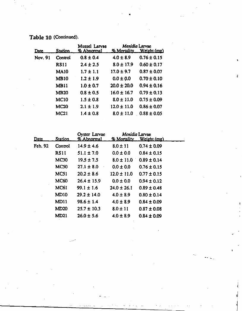
· tl

Menldla Larvae% Monality Wcjabt (ma>StationDate

Table 10 (Continued).

Mussel Larvae% Abnormal

Nov. 91 Control

RSllMAIOMB10

MB11MB20Me10MC20MOl

0.8 ±0.42.4 ± 2.51.7±1.11.2 ± 1.9

1.0 ± 0.70.8 ± 0.51.5 ± 0.82.1 ± 1.91.4 ± 0.8

4.0 ± 8.9 0.76 ± 0.1 58.0 ± 17.9 0.60 ± 0.17

17.0 ± 9.7 0.87 ± 0.07

0.0 ± 0.0 0.70 ± 0.1020.0 ± 20.0 0.94 ± 0.16

16.0 ± 16.7 0.79 ±0.138.0 ± 11.0 0.75 ± 0.09

12..0 ± 11.0 0.86 ±0.078.0 ± 11.0 . 0.88 ±0.05

Date StationOyster Larvae% Abnormal

MenldiQ Larvae% Mortality Wciabt (me)

Feb. 92 Control

RSllMC30MCSO

MCSIMC60MC61

MDJOMDllMD20MD2l

14.9 ± 4.651.1 ± 7.019.5 ± 7.527.1 ± 8.0

20.2 ±8.626.4 ± 15.999.1 ± 1.629.2 ± 14.098.6 ± 1.425.7 ± 10.326.0± 5.6

8.0 ± 11 0.74 ±0.090.0 ± 0.0 0.84 ± 0.158.0 ± 11.0 . 0.89 ±0.140.0 ± 0.0 0.76 ± 0.15

12.0 ± 11.0 0.77 ± 0.150.0 ± 0.0 0.94 ±0.12

24.0 ± 26.1 0.89 ± 0.484.0 ± 8.9' 0.80 ±0.144.0 ± 8.9 0.84 ±0.098.0 ± 11 0.87 ±0.084.0 ± 8.9 0.84 ±0.09

i

l'cill1b>lle lWlbSites exhibiting significant toxicity to test organisms in sediment elutriate tests from themarsh sUIVey. Data were analyzed by~OVA.

Test Series Species Sites Significantly More Toxic Sites Significantly More Toxic&Date Than Seawater Controls Than Reference Sites

Marsh #1 Bivalve All except MF22 (incl. Ref Sites) LM.MFIOJuly 91 Menidia LM 1M

Atherinops I...M. MF21 W. MF21

Marsh #2 All Tests None Significantly Different None Significantly Different

October 91

Marsh #3 All Tests None Significantly Different None Significantly Different

November 91

Marsh #4 Bivalve RSll. MDIO. MDll.lVilC61 MDII.MC61

February 92 Menidia MC61 MC61

Table 11 : Porewater concentrations of trace elements for gradient study

Pb Pb Ag Ag Zn Zn Cu Cu Cd Cd Ni Ni Mn MnCODE Station avg ppb SD avg ppb SD avg ppm SD avg ppb SD avg ppb SD avg ppb SD avg ppm SD

GDIO EVS04 shallow 142 108 6.7 7~9 31 13 509 200 85 30 6377 773 1940 616GD20 EVS04deep 77 22 6.3 4.6 10 3 379 187 20 17 2948 1037 467 46GDl~ Pt. Pinole piling shallo 148 70 12.9 13.0 242 414 3034 3131 329 162 6377 1736 4646 1163GD22 Pt.Pinole piling deep 80 83 27.2 44.4 34 9 284 142 182 185 3324 766 2137 81GD21 CC2deep 16 9 24.6 20.2 17 8 396 137 10 7 2364 477 969 146GD23 CC4deep 2 5 5.4 10.8 10 3 242 46 13 19 2474 315 1463 222CIJO Carr Inlet shallow 340 n=1 39.9 n=1 13 n=1 1651 n=1 139 n=1 2101 n=1 81 n=1CI20 ICarr Inlet deep 79 n=l 0.0 n=1 13 n=l 248 n=1 8 n=1 1174 n=1 494 n==l

Five field replicates for each station, except for Carr Inlet

" ..

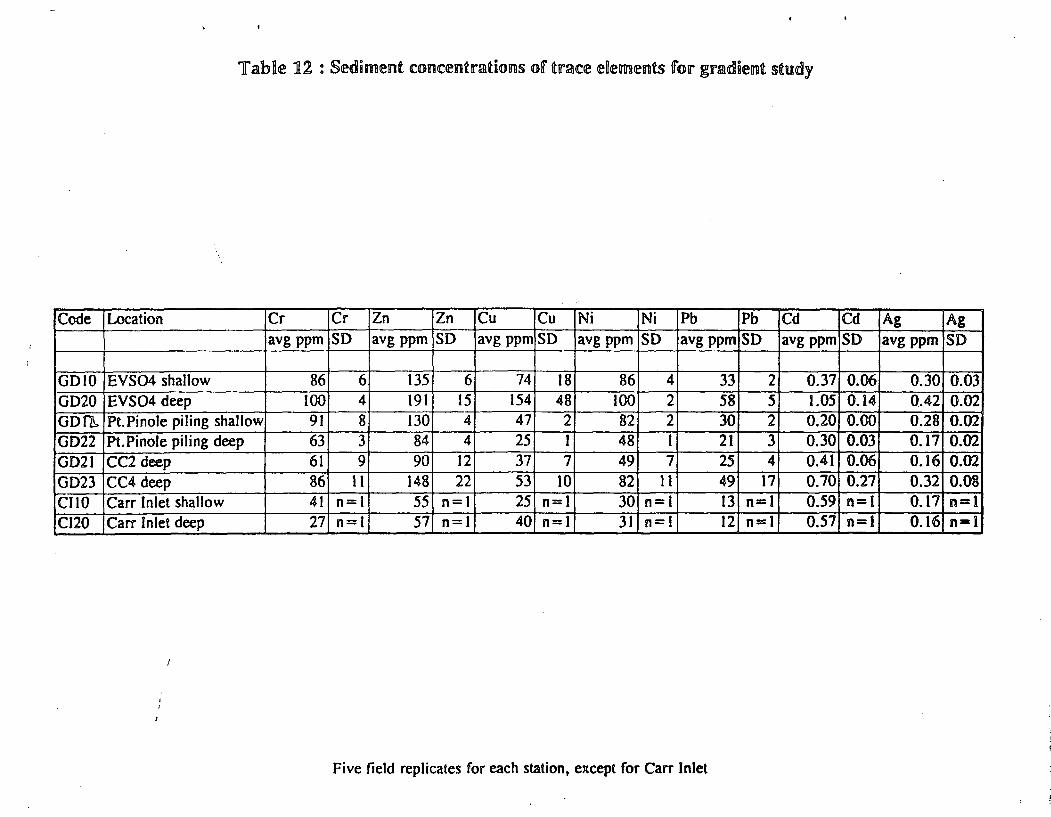
Code Location Cr Cr Zn Zn Cu Cu Ni Ni Pb Pb Cd Cd Ag Agavg ppm SO avg ppm SO avg ppm SD avg ppm SD avg ppm SO avg ppm SD avg ppm SD

GDIO EVS04 shallow 86 6 135 6 74 18 86 4 33 2 0.37 0.06 0.30 0.03GD20 EVS04 deep 100 4 191 15 154 48 100 2 58 5 1.05 0.14 0.42 0.02GDf], Pt.Pinole piling shallow 91 8 130 4 47 2 82 2 30 2 0.20 0.00 0.28 0.02GD22 Pt.Pinole piling deep 63 3 84 4 25 I 48 1 21 3 0.30 0.03 0.17 0.02GD21 CC2 deep 61 9 90 12 37 7 49 7 25 4 0.41 0.06 0.16 0.02GD23 CC4 deep 86 11 148 22 53 10 82 II 49 17 0.70 0.27 0.32 0.08ClIO Carr Inlet shallow 41 n=1 55 n=1 25 n=1 30 n=1 13 n=1 0.59 n=1 0.17 n=1CI20 Carr Inlet deep 27 n=1 57 n=1 40 n=1 31 n=1 12 n=1 0.57 n=l 0.16 n=1

Five field replicates for each station. except for Carr Inlet

Table ~3a Comparisons of various (actors affecting larval oyster toxicity test results from theCast:rO Cove gradient study. ANOVA tests were conducted using means for each field replicate(n=5). Comparisons between field replicates were made using laboratory replicates to define theANOVA error tenn.... Indicates significant differences.b Individual comparisons among sites are given below in Table 3c.

Comparison Samples Used in Comparison Probability"

Between Sites shallow layer. pore water 0.58

Between Sites deep core, pore water O.OOOI*b

Between Sites shallow layer, elutriates 0.24

Between Sites deep core, eJutriates 0.031j1b

Shallow layer (.38) vs Deep Core (.58) pore water, PP and EVS 04 0.35Shallow layer (.10) vs Deep Core (.15) elutriate, PP, EVS 04, and CC2 0.44

Pore water (.38) vs Elutriate (.11) shallow layer. PP and EVS 04 0.06

Pore water (.79) vs Elutriate (.13) deep core, PP, EVS 04, CC2 & CC4 0.0001·

Between Field Reps shallow layer, pore water, PP 0.0001·Between Field Reps shallow layer, pore water, EVS04 0.0001*Between Field Reps deep core, elutriate, CC2 0.03·

Between Field Reps all others >0.05

Table 13blndividual comparisons of sites within the gradient study indicate the following sites hadsignificantly greater toxicity than reference sites at p <0.05 using Dunnett's multiple comparisontest. The proportion abnonnal for each site is given in parentheses.

Type of SampleDeep Core, Pore Water

Deep Core. Elutriate

Reference Site0022 (0.17)

0022 (0.09)

Sites with Significant Toxicity

0020 (0.99)

0023 (1.00)

0021 (0.98)

(CI20 (1.00»

0020 (0.29)

' •• '. • " .... : ..... • ." ft ' ••• ~ ~.

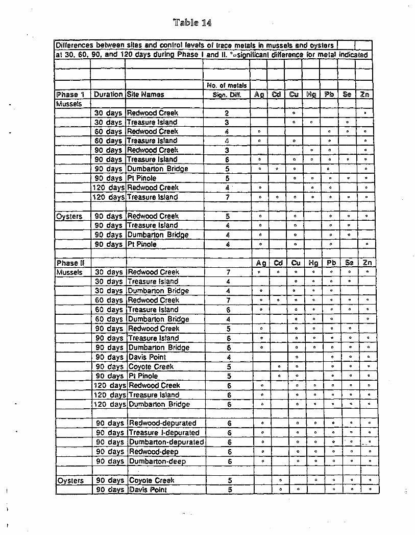
Differences between slles and control levels of trace metals In mussels SInd oysters I Iat 30, 60, 90, and 120 days during Phase I and II. °osionificant difference for metal indicated

No. of metalsPhase'il Duration Site Names Sign. om. Ag Cd Cu lHlCl !?(l) Ss 2nMussels

30 days Redwood Creek 2 .. •30 days Treasure Island 3 0 0 °60 days Redwood Creek ~ 0 0 0 °60 days Treasure Island t3 0 0 0 °90 days Redwood Creek 3 ° 0 °90 days Treasure Island 6 0 0 0 0 0 0

90 days Dumbarton Bridge 5 ° 0 0 0 °90 days Pt Pinole 5 ° 0 0 0 0

120 days Redwood Creek 4" ° 0 0 °120 days Treasure Island 7 0 0 0 0 0 0 °

Oysters 90 days Redwood Creek 5 ° 0 0 0 0

90 days Treasure Island ~ 0 .. 0 0

90 days Dumbarton Bridee 4 0 0 0 °90 days Pt Pinole 4 0 0 0 °

Phase II Aa Cd Cu Ilia Pb Ss 2nMussels 30 days Redwood Creek 7 0 0 0 0 0 0 0

30 days Treasure Island 4 0 0 0 0

30 days Dumbarton Bridge <4 0 .. 0 0

60 days Redwood Creek 7 .. .. .. .. 0 .. ..60 days Treasure Island 6 0 0 0 0 0 0

60 days Dumbarton Bridge <4 0 0 0 0

90 days Redwood Creek 5 0 .. 0 0 0

90 days Treasure Island 6 0 0 0 0 .. 0

90 days Dumbarton Bridge 6 0 0 0 0 0 °90 days Davis Point 4 0 0 0 0

90 days Coyote Creek 5 0 0 0 .. °90 days Pt Pinole 5 0 0 .. 0 0

120 days Redwood Creek 6 0 0 0 0 0 °120 days Treasure Island 6 ° 0 0 .. .. ..120 days Dumbarton Bridge 6 0 0 .. .. .. ..

90 days Redwood-depurated 6 0 0 0 .. 0 •90 days Treasure I-depUrated 6 .. 0 .. 0 " ..90 days Dumbarton-depurated 6 .. 0 0 0 0 0--.90 days Redwood-deep 6 0 0 0 0 0 0

90 days Dumbarton-deep 6 0 0 0 0 .. ..

Oysters 90 days Covote Creek 5 0 0 .. .. ..90 deWS Davis Point 5 0 0 .. 0 ..

I Table 15 ,I I ..

CONTAMINANTS IN SOllT'H. CENTRAL AND NORTH BAY MUSSElSMEAN MEAN MEAN PRErxMNANT'

CONTAMINANT SOUTH TREASl..AE I N:)RJH lleD-.

SLVE'R 0.305 0.345 0.15 NORlHLOWCAD.41lJ,,1 7.25 8.3 9.5 NORlH SUGHTlVHIGHwmt 10 12.5 12.1 C..." -_ NORTH SlIGHTlY HIGHM3=O..RV 0.25 0.295 0.235 N:N:LEAD 2.355 2.5 3.05 NOR'TH SUGHTlVHIGHSB..ENUM 1.75 3.1 2.65 NORTH. CENTRAL SlGHTlVHIGHZNC 230 230 230 N)\E

SUMOOT 226.5 68 92 SOUTHHGHSUM CH.OADANE 60.05 20.35 17 SOUTH HIGHSUMPAH 429.5 936 246.5 CENTRAL AND SOJTH HIGHSlA4PCB 391.5 213 86.5 SOl1TH AND CENTRAL HIGH

MEANS ARE FROM TWO VALUES (PHASE 1 AND PHASE II)

,,' . '.., ,," :", '.~, .....".' ~...". ..... , . .. ... .'" ..... .. .' ... ..",.

Table 16

RATIOS BE'TWE811 MUSSElS AND OYSTERS MEAN MEANMlBSB.S 0'r'STERS RAllO RATIO MU5SB..S 0¥SlERS RAllO RATIO

DOT 117 132 0.89 W'PER 13 240 0.0572 110 0.65 13 200 0.0758 97 0.60 7.5 253 0.0373 124 0.59 9 180 0.05

267 228 1.17 0.78 10 417 0.02 0.04~ 18 18 1.00 tJlRl.Rf 0.27 0.12 2.25

17 31 0.55 0.3 0.13 2.3119 20 0.95 0.2 0.13 1.5425 25 1.00 0.22 0.12 1.9392 70 1.31 0.96 0.2 0.2 1.00 1.79

SUVlPAHS 104 807 0.13 MANGANESE 26 49 0.53621 1905 0.33 26 76 0.34

99 773 0.13 23.6 95 0.25116 978 0.12 32 88 0.36859 1423 0.60 0.26 22.9 56 O.4f 0.38

SJMPalS 129 169 0.76 LEAD 2.2 0.52 4.23300 318 0.94 2.5 0.5' 4.90187 263 0.71 1.8 0.59 3.05252 299 0.84 , .9 0.54 3.52647 368 1.76 1.00 3.9 1.6 2.44 3.63

SlYER 0.2 5.9 0.03 SB...ENU\f 2.6 2.7 0.960.92 6.1 0.15 3 3.5 0.86

0.3 9.3 0.04 2.3 3.5 0.660.41 5.9 0.07 1.2 3.3 0.36

0.1 9 0.01 0.06 2.5 4.3 0.58 0.69~ 8.9 6.1 1.(16 IN; 260 HOO 0.24

7.6 6.6 1.15 260 1100 0.249.8 9 1.23 240 1400 0.17

7 7.9 0.90 250 900 0.2810.1 8.1 1.25 1.20 200 1133 0.18 0.22

~ 15 6 2.50 AlUMINUM 1433 410 3.50

'1 2.9 2,~~ 123~ 770 1.606.1 5 t .22 1400 940 2.199.7 , .8 5.39 1&33 953 '.714.9 4.1 1.17 2.63 1800 750 2.40 2.29

('J

Table 17

AIIdo8 ,..... 01 ......, _at ___81IDN at .... 01 o. 1.2. ,. and 4 fNnlhe In__ In ,.... , aid n"_Ill IOlnecl by ...... nIlt a!;roJfttl"'" llIIl.......

NJ CD OJ fa .. IE III.......~e-_ 0 I , 4 , 0 • 2 0 , 4 2 0 2 , • 0 I 4 , 0 4 , I 0 , • I

T_...."" 0 2 , • • I , 0 0 I 4 , 0 I • , 0 I • , 0 a , • 0 I • ,

.......2 • • , 0 I o , • I o • , I o , • 2 o , I • • , • I

t , •

I , •

• , I 0

• '01

o

o

I , •

I , •

o ., 2

O. I'

o I

o I

, 4

. ,

o • I • ,

-~=--

• I. ,

o

o

It.

t • ,

,...,. ......:,,","I to """"' ....,,,-, 0.0 t.O 1.0 1.0 '.0 ,.. 1.1 0.' '.a '.0 0.0 I.' '.0 I.' t.O 0.0 1.0 1.0 I.' ,.. 0.0 t.' t.' '.0 '.0 '.0 t.O '.0 '.0 '.0 •.• I.' '.0 •.• I.'"-I 0.0 t.7 t.7 1.7 '.0 '.0 '.0 0.7 I.' t.O 0.0 1.0 I.' ,., ,., 0.0 '.0 2.0 1.7 I.' 0.0 t.7 t.7 '.7 '.0 0.0 '.0 I.' ,., ,., 0.0 '.7 I.' '.01.7

o.-t 0.0 ••• t.' I.' '.0 ,.. 2.' 0.' 2.r '.0 0.0 t.' '.0 '.0 I.' 0.0 I.' 1.0 I.' I.' 0.0 t .• t.' , .• '.0 0.0 '.0 t.' '.1 '.1 0.' t.' 1.' 2.' I.'

.. .. .,

A P P E ~ 0 I X 0

Strategy for Establishing Sediment Quality Objecti~es

based on HUGan Health Risk Assess~nt

This report is the product of a contract between the State Water Board and theCalEPA Office of Environmental Health Hazard Assessment. In the future, theState Water Board will consider funding this strategy.

STRATEGY FOR

ESTAlBLISHTING SEDTIMENT QUALITY OJBmCTI'VES

BASED ON

HUMAN HEAlLm mSK ASSESSMEN1r

prepared by

Robert K. Brodberg, Ph. D.Karen Kan, Ph. D.

andGerald A. Pollock, Ph. D.

Office of Environmental Health Hazard AssessmentCalifornia Environmental Protection Agency

601 North 7th StreetP.O. Box 942732

Sacramento, CA 94234-7320

February 1993

PRElFACE

The California Legislature and Governor added Chapter 5.6, Bay Protection and ToxicCleanup (BPTC), to the state Water Code in an effort to protect the valuable resources withinthe estuarine waters and bays of the state. The BPTC section directs the State WaterResources Control Board (SWRCB) to formulate and adopt a plan to accomplish this goal(SWRCB, 1991). This plan is designated the Enclosed Bays and Estuaries Plan (EBEP).

One of the goals of the EBEP is to develop sediment quality objectives (SQO). Theseobjectives will supplement existing water quality criteria. Sediment quality objectives arebeing developed to protect aquatic life and human health from chemical contaminantsaccumulating in sediments. The Office of Environmental Health Hazard Assessment(OEHHA) in cooperation with theSWRCB is responsible for developing recommendations forSQO for California bays and estuaries. This document describes the scientific background anda proposed technical strategy for establishing SQO based on human health concerns.

_________________ 11 _

ACKNOWLEDGEMENTS

The strategy presented in this document reflects an ongoing collaboration between the Officeof Environmental Health Hazard Assessment (OEHHA) and the State Water Resources ControlBoard (SWRCB). Staff of the SWRCB and OEHHA have contributed to the present documentby gathering and reviewing information related to chemical contamination of fish andsediments. OEHHA acknowledges the contributions of these scientists in fonnulating thepresent strategy.

We also thank the following for their diligence in preparing this document: Ms. PatriciaHenry for preparing and organizing the text; Ms. Mercedes Danao for preparing the figure;and Ms. Shirley Brouillette for the tables. .

. --

----------------iii ...:.- _

TABLE OF CONTENTS

Page

PREFACE , ii

ACKNOWLEDGEMENTS ...............................................•............................. iii

TABLE OF CONTENTS iv

LIST OF FIGURES vii

EXECUTIVE SUMMARy ~.- viii

1.0 IN1"RODUCTION : 1

2.0 REGULATORY FOUNDATION FOR SETTING SEDIMENT QUALITYOBJECTIVES 2

3.0 APPROACH TO SETTING SEDIMENT QUALITY OBJECTIVES 5

4.0 SCIENTIFIC BACKGROUND FOR THE SEDIMENT QUALITY STRATEGy 5

4.1. Sediment Quality Objectives for Aquatic Life 5

4.2. Sediment Quality Objectives for Human Health 5

4.2.1. Human Risk Assessment 6

4.2.1.1. Maximum Tissue Levels in Seafood 7

4.2.2. Predicting Bioaccumulation 8

4.2.2.1. Methods for Estimating Bioaccumulation 9

4.2.2.1.1. Bioaccumulation Estimation from Bioconcentrationand Food-Chain Multiplier 10

4.2.2.1.2 Bioaccumulation Estimated from Field Data 10

4.2.2.1.3. Accumulation Factor Model of Bioaccumulation 11

4.2.2.1.4. Army Corps Dredging Model of Bioaccumulation ~- 1-2 -

4.2.2.1.5. Food-Web Equilibrium Model 12

_______________ IV _

Page.

4.2.2.1.6. Kinetic Models of Bioaccumulation :~ 12

4.2.2.1.7. Bioaccumulation Model for SQO Estimation 13

4.2.3. Analysis of Uncertainties for the Sediment QualityObjective Strategy 14

4.2.3.1. Human Health Risk Assessment.. 14

4.2.3.2. Predicting Bioaccumulation 15

5.0 STRATEGY FOR DETERMINATION OF SEDIMENT QUALITY OBJECTIVES 16

5.1. Contaminant Selection and Prioritization (Task 1).: 16

5.2. Human Health Risk Assessment (Tasks 2-4) 16

5.2.1. Hazard Identification and Dose-Response Assessment. 16

5.2.2. Exposure Assessment ; : 17

5.2.3. Calculation of Maximum Tissue Levels 17

5.3. Predicting Bioaccumulation (Task 5) 17.

5.3.1. Predicting Bioaccumulation Using PM 17

5.3.2. Predicting Bioaccumulation Based on the EqP Approach 17

5.3.3. Predicting Bioaccumulation Based on Food-Web Compartments ... 18

5.3.4. Predicting Bioaccumulation Based on a Kinetic Model 18

5.4. Critique of Predicted Bioaccumulation Factors and Sediment "!

Quality Objectives (Task 6) 18

5.5. Recommendation of Sediment Quality Objectives to the State WaterResources Control Board (Task 7) .' 18

6.0 SUMMARY ~;.. :.~ 18

. 7.0 REFERENCES , 20

--------....,....-------v-:-- -:-- _

" • •• .... '. •• •• "'•.~ <' .,. "':' ".' • r:""~'••: ••• ' •• '" ., , _" ~ _~. .' ..

-----'--_....:.-~....:.-_----------'--'---~-'----'--'--_._.=':'.'-'''' . ':..'\.,,~.,~ '.: ... - '.' " , " ~.' ." . "." ". ., .

Page

8.0 GLOSSARY OF TERMS 24

9.0 LIST OF ABBREVIATIONS AND ACRONYMS 28

10.0 APPENDICIES 29

APPENDIX 1 Examples of Estimated Human Health Risks from ContaminatedSeafood 30

APPENDIX 2 List of Priority Pollutants and 301(h) Pesticides ListedAccording to Structural Compound Class and Octanol/WaterPartition Coefficient. 31

_______________ vi ----'- _

FIGURE 1

LIST OF FIGURESPage

Pathways of Human and Wildlife Exposure through a SimplifiedAquatic Food-Web Due to Chemical Contamination of Sediments 4

r

.'

---------------- vii _

EXECUTIVE SUMMARY

This report describes the scientific background and a proposed technical strategy for settingSediment Quality Objectives for environmental chemicals in California based on human healtheffects in California. This strategy was developed by the Office of Environmental HealthHazard Assessment (OEHHA) in cooperation with the State Water Resources Control Board(SWRCB). The state Water Code requires that Sediment Quality Objectives (SQO) bedeveloped in conjunction with the Bay Protection and Toxic Cleanup program.

Sediment quality objectives are levels of a contaminant in sediment which will not result inpotentially unhealthy or hazardous levels of the contaminant in seafood (fish or shellfish) whenconsumed by humans, or which do not result in excessive environmental contamination (WaterCode Section 13391.5). SQO are based on and are intended to be predictive of biologicaleffects or tissue levels. SQO extend the process of protecting water quality by regulatingsediment as a reservoir for contaminants and recognize fish or shellfish ingestion as animportant route of exposure.

The following seven tasks comprise the strategy proposed by OEHHA to developrecommendations for SQO for human health effects in California.

I) Select contaminants of concern based on EPA lists. Prioritize contaminants ofconcern in California based on in-state use, toxicology profile, and Californiamonitoring data.

2) Identify appropriate cancer potency (q [*) or reference dose (RID) for the prioritizedcontaminants of concern identified above.

3) Develop human exposure scenarios considering potentially different patterns ofseafood consumption in California. Include alternative scenarios such as consumptionof finfish and/or shellfish; and consumption by sensitive subpopulations (e.g., fishers,children, ethnic groups).

4) Determine a maximum tissue level of chemical contaminant allowable in fish and/orshellfish tissue using the appropriate seafood consumption scenario(s) and potencyvalues identified above.

----.,.------------- viii ~ _

5) Use all appropriate bioaccumulation models to predict the accumulation of chemicalcontaminant from sediment to finfish and/or shellfish tissue.

6) Evaluate the bioaccumulation predictions by comparison to laboratory and field data.Based on the appropriate bioaccumulation value(s) calculate sediment levels that couldlead to the maximum tissue level identified above. Sediment levels calculated in thisway are proposed SQO based on human health effects.

7) Recommend the proposed SQO to the SWRCB for adoption. Include a discussion ofthe scientific basis and limits of certainty of this recommendation.

The Office of Environmental Health Hazard Assessment recommends adoption of this humanhealth-based strategy to develop SQO.

---------------- ix --:- _

1.0 INTRODUCTION

Chemical contaminants in the environment are a problem because they may reduce our qualityof life and may threaten human health. Contaminants may be merely noxious or have serioustoxic effects. Government agencies have addressed the problem of chemical contaminants inthe environment by setting standards and guidelines for important air and water bornecontaminants with the goal of protecting environmental quality and human health.

Sediments are a significant reservoir of environmental contaminants in aquatic environments(Dickson et al., 1987). At this time, regulatory controls for sediment-bound contaminantshave not been completely incorporated into existing water quality standards. Consequently,recent legislation has focused on developing guidelines for chemical contaminants insediments. These levels have been referred to as "sediment quality objectives" (SQO) inCalifornia (Water Code Section 13391.5), and "sediment quality criteria" (SQC) by the U.S.Environmental Protection Agency (EPA, 1991).

Human exposure to chemical contaminants in contaminated sediments is indirect via theconsumption of seafood. Seafood species may directly assimilate the chemical contaminantfrom sediment or indirectly via consumption of contaminated organisms from lower levels ofaquatic food-webs. This is the primary route through which humans can be exposed tochemicals present in the sediments, potentially leading to adverse health effects.

The purpose of developing SQO is to protect the broad scope of beneficial uses of California'scoastal waters. The accumulation of chemical contaminants in sediments in California's baysand estuaries presents a potential hazard to both aquatic life and human health. Separate SQOwill be developed for the protection of human health and aquatic life. Although both processesare related and equally important, the derived values may be very different. For a givenchemical and site, the lower SQO will protect both endpoints.

Contaminated sediments have already resulted in the contamination of seafood in severallocations in the United States. As an example, estimates of potential human carcinogenic risksfrom consumption of highly contaminated fish and shellfish range from 10-4 to 10-2 (seeAppendix 1). Health advisories regarding consumption of fish or shellfish in contaminatedlocations have been issued throughout the United States including southern California (pollocket al., 1991), Quincy Bay, Massachusetts (Reimold et al., 1988) and Puget Sound, Washington(Tetra Tech, 1988). These evaluations have been based on site-specific seafood tissue levelsdetected after extensive contamination had already occurred. There is a pressing need for theestablishment of regulatory standards for a wide range of chemicals and locations that can beapplied to prevent future contamination.

The objective of this report is to describe a strategy for developing such standards (SQO) forthe protection of human health. While it is clear that sediment-bound contaminants have led toundesirable levels in seafood (see Pollock et al., 1991), a formal process for regulating

contaminants in sediments has not been developed (Shea, 1988). Therefore, a strategy needsto be developed for establishing these levels.

2.0 REGULATORY FOUNDATION FOR SETTING SEDIMENT QUALITYOBJECTIVES

The regulation of chemical contaminants has focused on setting standards and criteria whichprotect humans from excessive exposure to the contaminants. Risk assessment methodology iscurrently used in this process (EPA, 1991). Using this methodology, acceptable exposurelevels can be established for likely environmental exposure routes (typically air and water),and measures can be identified to mitigate excessive exposure.

The regulation of chemical contaminants in the air, soil and water serves to protect not onlyhumans, but also other organisms from the toxic effects of these contaminants; Chemicalcontaminants in an environment can have far ranging adverse effects on organisms occupyingthat environment. Contaminants can have direct toxic effects on single organisms in theenvironment, either increasing or decreasing reproduction or survival. These direct individualeffects may cause changes in the ecosystem by changing population size, species compositionand etc. These changes may affect humans and wildlife that showed no direct toxic responseor had no direct exposure to the source of contaminant.

In aquatic environments, chemical contaminants can directly impact organisms in or on thesediments (Giesy et al., 1990) or those in the water column (Malueg et al., 1983). Theseenvironments may have four or five trophic levels in compl~x food-webs (Dickson et al.,1987). A variety of invertebrate and vertebrate benthic or pelagic organisms can be exposed

. by consumption of lower trophic level organisms and/or direct ingestion or absorption ofcontaminant. Humans or wildlife consuming these organisms as food can be indirectlyexposed to the contaminant and consequently may be put at risk of adverse health effects.Figure 1 shows an aquatic food-web tracing human exposure to a chemical contaminantintroduced into the aquatic environment.

.Federal regulations to protect aquatic environments are promulgated by the EPA and are basedon the premise that the beneficial uses of aquatic environments should be protected (EPA,1991). Protection includes aquatic organisms in these environments, and is extended toinclude the terrestrial organisms (e.g., humans) that use these environments. These aquaticorganisms must,not be adversely effected by exposures to a waterway. General water qualitystandards have been adopted by EPA which 'protect aquatic life and human health. Nationalwater quality criteria are the established means to translate narrative standards into numericvalues. These numeric criteria are used for the control of toxic pollutants in water. __ - ..

Individual states in turn adopt the general standards and objectives or customize them to meettheir specific needs. State procedures generally follow the basic principles used by the EPA

-----------------2 --- _

when adopting objectives to protect aquatic life and human health. Again, risk assessmentmethodology is presently the established foundation for deriving water quality criteria based onhuman health effects.

California has adopted regulatory standards and objectives for water quality (California WaterCode) and will extend them to include SQO (Water Code Section 13392.6 and 13393). TheState Water Resources Control Board (SWRCB) is responsible for the general development andimplementation of these objectives and related programs (Water Code Sections 13390 - 13396)such as the California Enclosed Bays and Estuaries Plan (EBEP). Related programs willutilize SQO to identify and prioritize toxic hot spots in California bays and estuaries.

The Office of Environmental Health Hazard Assessment is charged with formulating SQOrecommendations based on human health risk assessment (Water Code Sections 13393 and13395.5). In developing a SQO strategy, OEHHA has built upon the established process forsetting water quality criteria and incorporated relevant scientific information specific tosediments.

----------------3---------,---------

Humans & Wildlife ...(Seafood ......Consumption)

~~ .4~

Predatory Fish· ...""'I

~ ..

~I Forage· Fish and I~Invenebrates 1 !I~ ~ iI

II

I!

II . I- Phyto-plankton. Deairus ..... 1 Zoo-plankton I! ~I

i.4..

! I \I l

--------.( WATER >'-.'---r-....-....----:-------------

Ai· I

Benthic lnvenebrat~~~~~~~~~~~~~~~~~~~~~~~~~~~~~~~~I 14--" ~

. - I <CONTAMINANT )'------~ I_N_S_E_D_IM_E_NT __

Figure 1: Pathways of Human and Wildlife Exposure through a Simplified AquaticFood-web Due to Chemical Contamination of Sediments _

*

Arrows show movement of contaminant.

There may be more than one trophic level here.

----------------4 _

--------------------_. .- _.- - --.-. - -

3.0 APPROACH TO SETTING SEDIMENT QUALITY OBJECTIVES

The Office of Environmental Health Hazard Assessment proposes a technical strategy fordeveloping SQO recommendations for human health in California.· The strategy has beenorganized as a series of tasks for deriving SQO based on the methodologies of human healthrisk assessment and environmental fate modeling. These tasks include selecting andprioritizing contaminants of concern in California, setting maximum tissue levels for seafoodtissue, predicting bioaccumulation, estimating sediment contaminant levels (proposed SQO)leading to the protective tissue levels, and evaluating the accuracy of each proposed SQO. Theend product of application of this strategy will be a recommendation to the SWRCB foradoption of proposed SQO for selected chemical contaminants in sediments in California.

The scientific background for the strategy is presented below. This is followed by presentationof the seven basic tasks of the strategy.

~.o SCiENTIFIC BACKGROUND FOR THE SEDIMENT QUALITY STRATEGY

~.l. Sediment Quality Objectives For Aquatic Life

Washington State has established standards for regulating the quality of marine sediments byusing the apparent effects threshold (AET) approach (Washington State, Department ofEcology 1991). These AET values for chemical contaminants in sediment were developedbased on the level of contaminant which caused an acute or chronic toxic effect to sensitiveaquatic life forms in laboratory tests. Since toxicological effects in the AET approach dependon the environmental surroundings of a specific site, the sediment quality standards ofWashington State are applicable only to the site for which they were developed, in this casePuget Sound.

EPA recognizes the AET approach as a credible step towards development of sediment qualitycriteria (EPA 1989b). EPA is evaluating this approach and the equilibrium partitioning (EqP)approach (EPA, 1989b, and 1990) for use in setting sediment quality criteria. The EqP is alsobeing used to set contaminant levels in dredged materials (US Army Corps of Engineers andEPA, 1991). Thus far, these approaches have been applied to aquatic life. The SWRCB isalso evaluating the AET approach for setting aquatic life objectives.

~.2. Sediment Quality Objectives For Human Health

A standardized procedure for setting SQO based on human health effects has not beenestablished within the regulatory community (Shea, 1988). Any procedure to set SQ6-must- - _ .recognize the indirect nature of human exposure to sediment contamination and the complexrelationship(s) between contaminant levels in the sediment and in aquatic organisms at differenttrophic levels. The elements for a procedure can be developed by combining the risk

-----------------5 _

assessment process and models estimating the movement and bioaccumulation of chemicalcontaminants in aquatic ecosystems. These models are necessary to predict the sedimentconcentration of a contaminant that would lead to a given concentration in edible seafood.

Risk assessment and bioaccumulation modeling are based on different underlying assumptionsthat incorporate available biological data and facilitate prediction of specified endpoints. Bothare flexible and may incorporate options or methods that are more appropriate in differentsituations. This section reviews the scientific background for risk assessment andbioaccumulation modeling with emphasis on applications for deriving SQO. In addition, someof the underlying uncertainties in risk assessment and bioaccumulation modeling are discussed.Some of the uncertainties in bioaccumulation modeling may be reduced with the collection ofmonitoring data that can be used to calibrate and validate models.

4.2.1. Human Risk Assessment

Human risk assessment can be used to establish acceptable levels of contaminants underspecified exposure conditions (e.g., consumption o(:ontaminated seafood)(EPA, 1989a; NRC,1983; Pastorok, 1988). Risk assessment is the process for evaluating the toxicity of acontaminant and quantifying the potential harm (risk), if any, caused by exposure to thecontaminant. Risk assessment is usually divided into four discrete steps: hazard identification,dose-response assessment, exposure assessment and risk characterization (NAS, 1975; NRC,1983).

Hazard Identification (HI) is the determination of whether a particular chemical is or is notcausally linked to a particular adverse health effect. Cancer and non-cancer (e.g., birthdefects, nerve damage or organ dysfunction) endpoints are considered germane health effectsfor risk assessment. Hazard identification involves a qualitative determination of the toxicityof the contaminant. Pertinent health effects are observed in humans and/or experimentalanimals.

Dose-Response Assessment (ORA) is the determination of the relation between the magnitudeof exposure and the extent of biological response or the probability of occurrence of the healtheffects in question. ORA is the quantitative determination of the potency of a contaminant andmay vary with the route of exposure to the contaminant.

HI and DRA, combined, involve a complete review of the toxicology database, adetermination of the quality of the toxicology studies, and mathematical modeling of the dose­response data. The result of a ORA for a carcinogenic compound is the determination of acarcinogenic potency value (ql *) for the compound. The ql * can be used to estimate excesscancer risk due to exposure to a specified dose of the carcinogenic contaminant.A reference dose (RID), previously referred to ~ an acceptable daily intake (ADO, is usuallydetermined for non-carcinogenic toxicological endpoints (e.g., effects believed to have a

---------------- 6 _

threshold for response). The RID is defined as a daily level of exposure which can betolerated over a lifetime without anticipated adverse effects. The RID is usually determined byidentifying the No Observed Effect Level (NOEL) in animal studies and dividing this level byan uncertainty factor. The uncertainty factor is determined based on the quality, nature, andcompleteness of the database and usually ranges from 10 to 10,000. In some cases, the NOELmay be estimated using a newer approach for evaluating non-carcinogenic data, referred to asthe benchmark dose procedure.

Hazard identification and dose-response assessments of many common contaminants havealready been completed by various organizations such as OERRA, EPA, and the World HealthOrganization. OEHHA maintains a current listing of ql * values determined by Californiaagencies for many contaminants (OEHHA, 1992). The EPA Integrated Risk InformationSystem (IRIS) database also contains ql * and RID information.

Exposure Assessment (EA) is the determination of the extent of exposure before or afterapplication of regulatory controls. The route (e.g., oral, dermal or inhalation), the magnitude,frequency, and duration of exposure are considered in the EA. EA also requires identifyingthe population of health concern (usually a subpopulation with high exposure).

For SQO, the relevant exposure route is consumption of contaminated fish or shellfish. Thus,EA involves estimating human rates of seafood consumption and tissue concentrations ofchemical contaminants in the consumed seafood species. The relevant time-frame for exposuremay vary from a single meal to a lifetime depending on the identified health hazard. Acomprehensive EA would include other sources of exposure (e.g., air or water).

Risk Characterization (RC) is the description of the nature and often the magnitude of humanrisk, including attendant uncertainty. RC brings together the toxicity information from HI andDRA and the exposure information from EA to estimate the potential risks in a specifiedexposure situation.

4.2.1.1. Maximum Tissue Levels in Seafood

Risk assessment, therefore, can be used to calculate acceptable levels of a contaminant inseafood based on a given level of risk (e.g., 1 x 10-6 cancer risk). This major step in settingsediment quality objectives is similar to the EPA I S method for calculation of Reference TissueConcentrations (RTC) for seafood in their Technical Support Document for Water Quality­based Toxics Control (EPA, 1991). The SWRCB adapted EPA's RTC approach in calculatingMaximum Tissue Residue Limits (MTRL) for fish in the Pollutant Policy Document (1988).The difference between the derivation of RTC and MTRL is that MTRL focus on water as the _exposure source. The MTRL equation for carcinogens is:

_________________ 7 ~---------

MTRL (mg/kg) =RLxWT

q * x FC1

(1)

The corresponding MTRL equation for non-carcinogens is:

MTRL (mg/kg) =RID x WT

FC(2)

;

where:

RL =WT =ql* =FC =

risk level (e.g., 10-6),

standard weight of average human adult (70 kg),

cancer potency factor (mg/kg/dayr l ,

daily fish or shellfish consumption (kg/day),

Different values can be used to reflect the eating habits of different

target populations and,

RID = reference dose (mg/kg/day).

These equations will be adapted to develop maximum tissue levels for SQO for bays andestuaries.

4.2.2. Predicting Bioaccumulation

Deriving SQO requires determination of the concentration of contaminant in the sediment thatwould yield the maximum tissue levels. This involves following and predicting the movement·

. and accumulation of a chemical within bay and estuarine food-webs.

The movement and concentration of contaminants from the physical environment to the bio~ istermed bioaccumulation. In some cases, lower concentrations of contaminants accumulate inorganisms, but in many cases the observed concentrations in biota are higher than found in thephysical environment (Dickson et al., 1987; Young, 1988). Quantitative models fordescribing the bioaccumulation of a chemical contaminant have been developed. Generally, ..these models have ·described the property of bioaccumulation as a function of bioconcentrationand other related factors. Bioaccumulation estimates from these models can be used in reverseto calculate sediment levels corresponding to tissue concentrations. These calculated sedimentlevels are derived SQO.

Aquatic organisms can bioaccumulate chemical contaminants from either the water phase orthe solid (particulate and/or sediment) phase (Dickson et al., 1987). Sediments are composed

-- ------------- 8 --,. _

-, •• i "~'':'~' ;. .~'~M:"~".",'. ,. .. ..' .-" ~." '." .... ~ . :;'!'

of a particle phase and an interstitial water phase (pore water). Chemical contaminants tend toeither associate more with water or be bound more closely with particles. Ionic and watersoluble compounds tend to be dissolved in the water. Nonionic or neutral organic compoundstend to be more tightly bound to the particles.

Compounds which are associated with particles or are themselves particles may settle out ofthe water into the sediment. Over time, the accumulated total mass of a contaminant insediment can become much greater than the amount dissolved in the overlying water column.Thus, sediments act as an important reservoir for particle-bound chemical contaminants inaquatic environments (Morel and Schiff, 1983).

Bioaccumulation specifically due to exposure to the water column is designatedbioconcentration and is expressed as a bioconcentration factor (BCF). This form ofaccumulation is defined as the concentration of the chemical in tissue divided by theconcentration in the water column (EPA, 1980; 1991)." BCF can be determined in relativelysimple laboratory tests.

In sediments, benthic organisms are exposed to contaminants within the pore water and byingestion of sediment particles. These organisms can bioaccumulate concentrations of thechemical above the level predicted based on the BCF because they also ingest sediment-boundcontaminants (Dexter and Field, 1989). Similarly, organisms higher in the food-web whichconsume (ingest) contaminated benthic organisms can bioaccumulate levels of contaminantabove that estimated by BCF (Thomann and Connolly, 1984). The total bioaccumulation viaall routes is called the Bioaccumulation Factor (BAF). (See Figure 1 for a diagram of asimplified aquatic food-web.)

4.2.2.1. Methods for Estimating Bioaccumulation

A number of mathematical equations and models using field or laboratory data have beendeveloped to predict the bioaccumulation potential or tissue concentration of contaminantsassociated with sediments or water. These models follow two general approaches:equilibrium-based models and kinetic models. Equilibrium models assume that a chemicallybased equilibrium will be reached for any contaminant within components of the system beingsampled and modeled. The equilibrium approach focuses on the partitioning of chemicalsbetween sediment and benthic organisms assuming that thermodynamic equilibrium existsbetween the sediment and the organisms in the sediment (Lake et al., 1987; McFarland, 1984).This approach simplifies data requirements for these models. Theoretically, equilibrium basedmodels can predict the concentration of non-polar organic chemicals in an organism(bioaccumulation) given a known concentration of chemical in the sediment (Lee, 1992; Tet(a, _Tech, 1985). These models may prove especially useful as screening tools or for organisms atspecific levels in the food-web. The first five models presented below are equilibrium-basedmodels.

-----------------9 _

Kinetic models are needed to predict contaminant movement in complex and variableenvironments in greater detail. These models do not assume equilibrium conditions within thesystem. Simple kinetic models do assume that steady-state conditions exist, while morecomplex forms can model non-steady-state conditions such as those associated with varyingexposures. Kinetic models are based on rates of flux between physical (e.g. organism:water)or physiological compartments (e.g. blood:liver). Most of the fate models used to expressbioaccumulation are undergoing further development and validation (Lee, 1992; Tetra Tech,1985).

4.2.2.1.1. Bioaccumulation Estimation from Bioconcentration andFood-Chain Multiplier

EPA (EPA 1991) has used the bioconcentration factor (BCF) of a chemical contaminantcoupled with an estimated food-chain multiplier (FM) to predict the accumulation of persistentorganic compounds in fish tissue. BAF is then equal to a food-chain multiplier times thebioconcentration factor as shown by the equation:

BAP = FM x BCF (3)

FM values for this equation have been derived by Thomann (1989) based on a four levelfood-chain model. An expanded table of these food-chain multiplier values estimated fromn-octanol/water partition coefficient is given by EPA (U.S. EPA. 1991).

4.2.2.1.2. Bioaccumulation Estimated from Field Data

The BAF for an organism measured in its environment is expressed a~ the ratio of theconcentration of chemical contaminant in the organism I s body to the concentration of thechemical in the exposure source. The general form of this equation has been proposed byThomann et al. (1992) as the Biota Sediment Factor (BSF). This is an expression ofbioaccumulation specifically from a sediment source, and includes accumulation via ingestion.The BSF is not specific to benthic organisms.

BSF = Cb,L /Cs,oc (4)

where:

Cb,L = the lipid-normalized chemical concentration in the organism (b), and

Cs,oc = total organic carbon-normalized chemical concentration in sediment (s)'

10 _

; .. '

---------- ._ •• • 0_-

... ~ r';' •

This relationship can be used to generate BSF values from fish, shellfish and sedimentmonitoring data. In some cases, sufficient California monitoring data may be available for achemical to calculate this bioaccumulation factor. In such cases, the modeling discussed belowmay be unnecessary for specific chemicals or organisms. Monitoring information can alsoprovide data points for evaluation of the accuracy of modeling.

Equations 5 and 6 below are specific modifications of this general equation.

4.2.2.1.3. Accumulation Factor Model of Bioaccumulation

The Accumulation Factor (AF) model is essentially a laboratory based formulation of the BSFmodel. It is also referred to as the equilibrium partitioning approach (EqP). Like the BSFmodel, it assumes that chemical contaminants exchange freely between the organic carbon indifferent sediments and the lipids in different organisms. The AF model includes normalizingsediment for its total organic content and normalizing benthic organisms for total lipid content(Bierman, 1990; Ferraro et al., 1990). Partitioning based on this approach was found to yielda theoretical accumulation factor that was similar to those calculated from laboratory and fielddata (Rubenstein et al., 1987). This Accumulation Factor (AF) is expressed as follows:

AF = (CtJL)/(Cs/TOC)

where:

Ct = tissue concentration at equilibrium (ug/g dry wt),

L = lipid concentration of organism (gig dry wt),

Cs = sediment concentration (ug/g dry wt), and

TOC = total organic carbon in sediment (gIg dry wt).

(5)

Calculating an equilibrium-based AF is very promising for setting sediment quality criteria fornonionic organic chemicals in benthic organisms (Oi Toro et al., 1992), and EPA isconsidering using this approach. This approach yielded conservative estimates of tissueconcentrations (Ferraro, 1990; and Bierman, 1990) when applied to selected neutral organicchemicals. Its applicability to other groups of contaminants (e.g., metals, ionic compounds,etc.) and to non-benthic 'organisms is not as well established and should be further tested.

11

4.2.2.1.4. Anny Corps Dredging Model of Bioaccumulation

A modified EqP approach has been used by the US Army Corps of Engineers and EPA (1991)as a screening tool to estimate the Theoretical Bioaccumulation Potential crBP) ofcontaminants in dredged material. TBP in this model is the tissue concentration, and atheoretically-based constant [4] is equivalent to the AF in equation 5. TBP is expressed as:

TBP = 4 (Cs/TOC) / L

where:

TBP = tissue concentration based on whole-body wet-weight,

Cs = sediment concentration,

(6)

TOC = total organic carbon content of sediment, and

L = species lipid content as a decimal fraction of whole-body wet-weight.

Again, this model is expected to work best for nonionic organic chemicals and benthicorganisms.

4.2.2.1.5. Food-Web Equilibrium Model

Thomann (1989) used an equilibrium-based model to calculate the concentrations of organicchemicals in different compartments of a simple aquatic food-web. However, this model didnot include benthic organisms. Thomann et al. (1992) and Connolly (1991) have extendedsimilar models to successfully predict tissue concentrations in organisms in complex food-websthat include benthic and non-benthic organisms. These models solve for a series ofaccumulation factors (from water or sediment), one for each trophic level. Each accumulationfact0r is dependent on an uptake rate divided by the sum of an elimination rate and a growthrate. Rates are assumed to be at steady-state. Additional equations are presented to estimaterates based on physiochemical properties (e.g., n-octanollwater partition coefficient [Kow)):

4.2.2.1.6. Kinetic Models of Bioaccumulation

...

The kinetic approach views bioaccumulation as resulting from the dynamic uptake andelimination of a contaminant between different parts (compartments) of the system. Kineticmodels therefore are based on the rate of movement of the contaminant between .compartments. These models can be simple so-called first-order one-compartment ~Odels(cf. Davies and Dobbs, 1984) or very complex multi-compartment models; so-calledbioenergetically-based toxicokinetic models (cf. Landrum, 1989). These models may assume a

12 ~__~ _

:.~ ",:..:'. ,.

linear relationship for the rates (which means that threshold processes may be misrepresented),or more complex non-linear relationships can be used.

In the first-erder one-compartment model, bioaccumulation is essentially the ratio between therate of uptake of a chemical and its elimination rate (elimination includes metabolism andexcretion) over infinite time. These rates are assumed to be constant and not a function ofsediment concentration, tissue concentration, or exposure route. The rates are, however,dependent on factors which alter uptake or elimination such as differences in bioavailability,physiology, or feeding patterns of different organisms. Essentially this model views theorganism as a compartment with one input and one elimination rate (Lee, 1992; Tetra Tech,1985).

The bioenergetically-based toxicokinetic models incorporate more compartments and rates forprocesses within the system than the one-compartment models. As an example, thebioavailability or absorption of a contaminant in a specific sediment can be a variable in thismodel (Lee, 1992; Tetra Tech, 1985). Rates used in these models can be estimated, andcomplex models have successfully estimated observed BAF within an order of magnitude.

4.2.2.1.7. lBioaccumulation Model for SQO Estimation

Ultimately, the choice of which model should be used when setting sediment quality objectiveswill depend on which model more accurately predicts bioaccumulation given available data.The EqP approach requires less data but may not be applicable to all contaminants ororganisms. The kinetic approach may be more useful for certain contaminant groups such asmetals whose chemical characteristics are difficult to generalize. Despite differences, Clarket al. (1990) showed that the equilibrium and kinetic models are just different ways ofexpressing the same phenomenon. They also show the importance in any model of accountingfor differences in bioacccumulation between uptake from food and uptake from water.Variations on both models need to be investigated to determine situations where they work bestin California.

A number of general factors will affect the accuracy of bioaccumulation modeling regardlessof model choice. These factors include: physical and chemical properties of the contaminants(e.g., octanol/water partition coefficient); environmental characteristics (e.g., sedimentorganic carbon, pH and temperature); and differences between species composition of thefood-web in an environment (Tetra Tech, 1985). Physical and chemical properties determinethe bioavailability of a particular contaminant. Chemical contaminants with log octanol/waterpartition coefficients (log Kows) below two are highly soluble in water or are rapidly __metabolized and generally do not accumulate in fish. Contaminants with log Kows aboveseven are so tightly bound to sediments that they do not accumulate in the food-web (Connelland Miller, 1984). Environmental characteristics such as pH can alter the bioavailability ofsome chemicals by affecting the ionic state of metals and their movement and toxicity. And

13 ----------------

high organic carbon content in the sediment will increase the sediment's holding capacity fornon-polar organic chemicals. Identical or similar organisms may bioaccumulate differentconcentrations of contaminant due to differences in the species composition and complexity ofthe food-web (Lake et al., 1990).

4.2.3. Analysis Of Uncertainties For The Sediment Quality Objective Strategy

"Although risk assessment and bioaccumulation modeling are based on sound scientificprinciples, it is recognized that uncertainties are introduced by the underlying assumptions andextrapolations involved in these processes. Additional uncertainty and errors may beintroduced by poor quality or inappropriate data. The discussion below identifies some of theways in which uncertainty may be introduced into the process of setting SQO. Recognition ofthese areas of uncertainty is constructive for identifying weaknesses in the process and areas inwhich the process can be improved, and is an integral part of the SQO strategy.

4.2.3.1. Human Health Risk Assessment

The risk assessment process involves making assumptions and extrapolations which createuncertainties in the estimation of acceptable tissue levels (NAS, 1975; NRC, 1983). One ofthe more general assumptions is that the effects caused by a chemical in experimental animalscan predict the possible effects caused in humans. This affects both hazard identification anddose-response assessment. Another more controversial assumption is that the carcinogeniceffects caused by a chemical at high doses will also occur at much lower doses and that theprobability of this occurrence can be extrapolated ba~edon the magnitude of exposure. Theseassumptions affect the dose-response assessment step in risk assessment. The assumptions inthis step of risk assessment are based on toxicological data and hypotheses. They are subjectto evolving interpretations of scientific knowledge which in some cases may result in changingexisting ql * or RID values.

The most significant source of uncertainty in the exposure assessment step of risk assessment. isthe estimation of fish consumption rate (EPA, 1989a, and 1991). Exposure assessmentinvolves determining the dose of chemical contaminant that an individual is exposed to byconsuming contaminated fish. This assessment is primarily based on two factors: (1) theconcentration of chemical contaminant in specified fish tissues and (2) the amount of specified 't

fish tissues consumed. In determining SQO the chemical contaminant concentration in fishtissues is determined by setting the risk and therefore the amount of fish tissue consumed is theonly variable.

-The amount of fish consumption is difficult to estimate because adequate relevant data are notavailable. It is-clear that for some people fish may be a large part of their diet, while othersmay rarely eat any seafood. In reality, a number of subpopulations with different consumption

14 -:-- _

--------------------------

behaviors exist, but for convenience and consistency a single average exposure has often beenused. Estimates most pertinent to setting SQO for California bays and estuaries would bespecific to fish consumption in the state and include different ethnic or other sensitive orvulnerable subpopulations (i.e., pregnant women, children). At least one study would directlyapply to California (Puffer et al., 1982). Unfortunately, this study may be outdated, and itonly determined fish consumption for pier anglers.

Overall, the existing data allow some reasonable best estimates of fish consumption to bemade. However, developing alternative scenarios specifically for finfish or shellfish or forsensitive subpopulations (e.g. fishers or children) should be pursued.

The Office of Environmental Health Hazard Assessment presently uses an exposure scenariothat assumes an individual consumes 23 grams per day of seafood (DRS, 1989). Aconsumption rate of 23 grams per day is equivalent to 18.7 pounds per year, 1. 6 pounds permonth, or roughly one meal (about 6 ounces) per week. This consumption rate is consideredto be a minimum for active anglers and higher consumption rates may be more representativeof anglers (DHS, 1989; Puffer et aI., 1982). It should be noted, however, that estimates ofaverage consumption ranging from 23 to 40 grams per day do not change the calculation oftissue levels by a significant amount. Such calculated levels would vary by less than a factorof two.

4.2.3.2. Predicting Bioaccumulation

Uncertainties can be introduced in the bioaccumulation modeling step due to inappropriate orun met assumptions (Lee, 1992; Tetra Tech, 1985). Each model is most sensitive to variationsin its own set of assumptions. For example, the EqP model will not be accurate when theequilibrium assumption is not met while collecting laboratory data (i.e., data are used fromexperiments which are conducted for less time than necessary for equilibrium to be reached).Poor quality data used to model bioaccumulation can also introduce uncertainty. Laboratoryand field collected data can add different types of uncertainty. Laboratory tests cannotsimulate the complexity of real field situations. This will introduce uncertainty whenestimating bioaccumulation in a real food-web. One source of uncertainty in field generateddata is the assumption that all tissue contamination is due to a constant exposure level at asingle site. When contamination is unevenly distributed or when fish move within largegeographical areas this assumption will be violated.

The magnitude of the uncertainty will be established as these models are tested for specific

situations.

15 ...,......... _

5.0 STRATEGY FOR DETERMINATION OF SEDIMENT QUALITY OBJECTIVES

The OEHHA has divided the elements of the strategy for settingSQO into a series of tasksnecessary for implementation. These tasks are discussed below.

5.1. Contaminant Selection And Prioritization (Task 1)

The selection of contaminants is guided by federal r~quirements under the Clean Water Actwhich directs the states to set criteria for Section 307(a) priority pollutants for which EPA haspublished Section 304(a) criteria. A listing of some priority pollutants and 301(h) pesticides isincluded in Appendix 2.

Task 1: The OEHHA will establish a listing of contaminants for developingCalifornia SQO based on human health. Criteria for listing include comparingthe EPA priority pollutants with California usage and monitoring data onchemical contaminants in bay and estuarine sediments in order to identify thechemicals most frequently discharged and detected in California sediments.Additional factors to be considered in the process of identifying and prioritizingthe chemicals of concern will be the potential for bioaccumulation (e.g., Kow),toxicological concern'(e.g., potency), and the concentrations in sediments.

It is anticipated that this prioritized list of chemical contaminants of concern will be similar tothe list included in the Pollutant Policy Document (1988) for which MTRL have been derived.

5.2. Human Health Risk Assessment (Tasks 2-4)

Human health risk assessment will be used in the SQO strategy to calculate maximum tissuelevels of contaminants. The steps in human risk assessment are relatively straight-forward asdescribed earlier, but interpretation of the data requires profession'al judgement. Tissue levelswill be calculated that correspond to some specified level of health risk. The OEHHA willchoose appropriate risk levels based on the toxicological properties of each contaminant and'health policy considerations.

5.2.1. Hazard Identification And Dose-response Assessment.,'

TASK 2: Appropriate q I * and/or RID values will be added to the prioritiZedlisting of chemicals developed in Task 1.

---------------- 16 _

(

I

5.2.2. Exposure Assessment

Appropriate fish consumption rates must be developed in order to calculate numeric SQObecause consumption rate is a major determinant in the equation for calculating maximumtissue levels.

TASK 3: Consumption scenarios for finfish and shellfish and for sensitivesubpopulations (e.g., fishers or children) will be developed as appropriate.

5.2.3. Calculation of Maximum Tissue Levels

TASK 4: Maximum tissue levels will be determined for the prioritized list ofchemicals using the cancer potency (q, *) or reference dose (RID) values andconsumption scenarios identified above.

5.3. Predicting Bioaccumulation (Task 5)

A critical step in the process of developing SQO is the determination of BAF using one of themodels discussed above. Presently, there is limited consensus regarding the best model forestimation of bioaccumulation.

BAF for the prioritized list of chemicals will be calculated using selected models and theresulting values evaluated. There are differences between these models that may make onemore applicable under specific conditions (e.g., for metals vs. organics). These conditionswill be examined and described and only applicable models will be used for a given chemical.

5.3.1. Predicting Bioaccumulation using FM

TASK 5a: BAF will be determined using equation 3 described in section4.2.2.1.1. which is based on food-chain multipliers.

5.3.2. Predicting Bioaccumulation based on the EqP Approach

TASK 5b: BAF will be determined based on the equilibrium models expressedin equations 4, 5, and 6. The BSF, AF, and TBP variations on this model aredescribed in section 4.2.2.1.2, 4.2.2.1.3, and 4.2.2.1.4. The appropriateequation will be selected based on the available input data.

17 _

5.3.3. Predicting Bioaccumulation based on Food-Web Compartments

TASK 5c: BAF will be determined using the food-web model equations ofThomann et al. (1992) described in section 4.2.2.1.5.

5.3.4. Predicting Bioaccumulation based on a Kinetic Model

TASK 5d: BAF will be determined using kinetic model equations like those ofClark et al. (1990) described in section 4.2.2.1.6.

5.4. Critique of Predicted Bioaccumulation Factors and Calculation of SedimentQuality Objectives (Task 6)

The results of the above calculations of BAF (Task 5) will be evaluated to determine the mostappropriate methods for application in California. Models will be evaluated based onconcordance of their predictions with known laboratory or field measurements' ofbioaccumulation. This critique will include identification of the main sources and estimatedmagnitude of uncertainty in the human risk assessment and the estimation of BAF. The mostappropriate BAF will be used to calculate a sediment level corresponding to the maximumtissue concentration.

TASK 6: The results of this evaluation will be the identification of the mostappropriate BAF based on available data. The evaluation will also includerecommendations for further development and refinements in the process. Theselected BAF will be used to calculated a proposed SQO.

5.5. Recommendation of Sediment Quality Objectives to the State Water ResourcesControl Board

TASK 7: OEHHA will recommend to the SWRCB adoption of the proposedSQO derived as described above. The recommendation will include a summaryof the scientific basis for selection of the BAF and corresponding SQO anddiscussion of related uncertainty.

6.0 SUMMARY

The Office of Environmental Health Hazard Assessment has developed a strategy for-- _development of sediment quality criteria in cooperation with the State Water ResourcesControl Board. The OEHHA recommends that the SWRCB adopt this strategy for

. development of SQO to protect human health. The strategy combines elements of human

18 --'- ~__

health risk assessment with methods for assessing bioaccumulation of contaminants insediments. It includes an evaluation of methods and uncertainties that should be addressedbefore the adoption of California numeric SQO.

Once developed these SQO can be applied to the regulation of chemical contaminants inaquatic sediments, to the identification of toxic hot spots, and to protect the overall beneficialuses of the bays and estuaries of California.

19 -'-- _

7.0 REFERENCES

Bierman, V.I. 1990. Equilibrium partitioning and biomagnification of organic chemicals inbenthic animals. Environ. Sci. Technol. 24: 1407-1412.

Clark, K.E., F.A.P.C. Gobas, and D. Mackay. 1990. Model of organic chemical uptake andclearance by fish from food and water. Environ. Sci. Technol. 24: 1203-1213. •

Connell and Miller. 1984. Chemistry and Ecotoxico!ogy of Pollution. John Wiley & Sons,Inc. New York.

Connolly, J.P. 1991. Application of a food chain model to polychlorinated biphenylcontamination of the lobster and winter flounder food chains in New Bedford Harbor.Environ. Sci. Technol. 25:760-770.

Davies, R.P., and A.J. Dobbs. 1984. The pr~iction ofbioconcentration in fish. Wat. Res.18: 1253-1262.

Department of Health Services (DHS). 1989. Recommendations to the State Water ResourcesControl Board regarding Levels of Fish Consumption. Letter from Dr. K.W. Kizer,Department of Health Services, to Mr. I.W. Baetge, State Water Resources Control Board,September 28, 1989.

Department of-Health Services (DHS). 1991. A Study of the Chemical Contamination ofMarine Fish from Southern California. I. Pilot Study. Health Hazard Assessment Division,California Department of Health Services.

Dexter, R. and I. Field. 1989. A discussion of sediment PCB target levels for the protectionof aquatic organisms. Oceans 89. 2:452-456.

Dickson, K.L., A.W. Maki and W.A. Brungs (Eds.), 1987. Fate and Effects of Sediment­bound Chemicals in Aquatic Systems. Pergamon Press, New York, 445 pp.

Di Toro, D.M., C.S. Zarba, DJ. Hansen, WJ. Berry, R.C. Swartz, C.E. Cowan, S.P.Pavlou, H.E. Allen, N.A. Thomas, and P.R. Paquin. 1991. Technical basis for establishingsediment quality criteria for nonionic organic chemicals using equilibrium partitioning.Environ. Tox. Chern. 10:1541-1583.

EPA. 1980. Water' Quality Criteria Documents; Availability. Federal Register Vol. 45, No.231, Part V pp. 79318-79379.

EPA. 1988. Analysis of Risks from Consumption of Quincy Bay Fish and Shellfish.Environmental Protection Agency. Water Management Division, Region 1. Boston, MA.

EPA. 1989a. Assessing Human Health Risks from Chemically Contaminated.fish andShellfish: a Guidance Manual. Environmental Protection Agency, Office of Marine andEstuarine Protection, Washington, D.C. EPA-503/8-89-002.

---------------- 20 ......- _

-----~----------------------_. -._----.-----

EPA. 1989b. Evaluation of the Apparent Effects Threshold (AET) Approach for assessingSediment Quality. Report of the Sediment Criteria Subcommittee. A Science Advisory BoardReport. U.S. Environmental Protection Agency, Washington, D.C. EPA-SAB-EETFC-89­027.

EPA. 1989c. Risk Assessment Guidance for Superfund. Volume I. Human HealthEvaluation Manual (Part A). Office of Emergency and Remedial Response. U.S.Environmental Protection Agency, Washington, D.C. EPA/540/l-89/002.

EPA. 1989d. Risk Assessment Guidance for Superfund. Volume II. EnvironmentalEvaluation Manual. Office of Emergency and Remedial Response. U.S. EnvironmentalProtection Agency, Washington, D. C. EPA/540/l-89/001.

EPA. 1990. Evaluation of the Equilibrium Partitioning (EqP) Approach for assessingSediment Quality. Report of the sediment criteria subcommittee of the ecological processesand effects committee. A Science Advisory Board Report. U.S. Environmental ProtectionAgency, Washington, D.C. EPA-SAB-EPEC-90-006.

EPA. 1991. Technical Support Document for Water Quality-based Toxic Control. Office ofWater. U.S. Environmental Protection Agency, Washington, D.C. EPA/505/2-90-001March 1991.

Ferraro, S.P., H. Lee II, R.J. Ozretich, and D.T. Specht. 1990. Predicting bioaccumulationpotential: a test of a fugacity-based mode!. Arch. Environ. Contam. Toxicol. 19:386-394.

Giesy, J.P, C.J. Rosiu, R.C. Graney and M.G. Henry. 1990. Benthic invertebrate bioassayswith toxic sediment and pore water. Environ. Toxico!. Chern. 9:233-248.

Lake, J.L., N.J. Rubenstein, H. Lee II, C.A. Lake, J. Helthshe, and S. Pavignano. 1990.Equilibrium partitioning and bioaccumulation of sediment-associated contaminants by infaunalorganisms. Environ. Toxico!. Chern. 9: 1095-1106.

Lake, J.L., N. Rubinstein, and S. Pavignano. 1987. Predicting bioaccumulation:Development of a simple partition model for use as a screening tool for regulating oceandisposal of wastes. Pp. 151-166 in K.L. Dickson, A.W. Maki, and W.A. Brungs (eds.), Fateand Effects of Sediment-Bound Chemicals in Aquatic Systems. Pergamon Press, New York,NY.

Landrum, P. F. 1989. Bioavailability and toxicokinetics of polycyclic aromatic hydrocarbonssorbed to sediments for the amphipod Pomoporeia hoyi. Environ. Sci. Tech. 23:588-595.

Lee II, H. 1992. Models, Muddles, and Mud: Predicting Bioaccumulation of Sediment­Associated Pollutants. Pp. 267-293 in G.A. Burton (ed). Sediment Toxicity Assessment.Lewis Publishers, Ann Arbor.

Malueg, K.W., G.S. Schuytema, J.H. Gakstateer, and S.F. Krawczyk. 1983. Effect ofHexagenia or Daphnia response in sediment toxicity tests. Environ. Toxicol. Chern 2:73-82.

________________ 21 ...,.- _

McFarland V.A. 1984. Activity-based evaluation of potential bioaccumulation fromsediments. Pp. 461-467 in Dredging and Dredged Material Disposal. Vol. I. RoL.Montgomery and J.W. Leach (eds.). American Society of Civil Engineers, New York.

Morel, F.M.M., and S.L. Schiff. 1983. Geochemistry of Municipal Waste in CoastalWaters. Pp. 249-421. In Ocean Disposal of Municipal Wastewater: Impacts on CoastalEnvironment. Vol. 1. E.P. Meyers and E.T. Harding (eds). Sea Grant ColIege Program,MIT, Cambridge, MA.

National Academy of Sciences (NAS). 1975. Prin~iples for Evaluating Chemicals in theEnvironment. Washington, D.C.

National Research Council (NRC). 1983. Risk Assessment in the Federal Government:Managing the Process. The committee on the Institution of Means for the Assessment ofCrisis to Public Health, Washington, D.C.

Office of Environmental Health Hazard Assessment. 1992. California Cancer PotencyFactors. Standards and Criteria Work Group (June memo).

Pastorok, R.A. 1988. Guidance Manual for Assessing Human Risks from ChemicallyContaminated Fish and ShelIfish. PTI Environmental Services, Bellevue, WA.

Pollock, G.A., Y.A. Weider, I.J. Uhaa, A.M. Fan, and R.R. Cook. 1989. Risk Assessmentof Dioxin Contamination of Fish. California Dep'artment of Health Services.

Pollock, G.A., 1.1. Uhaa, A.M. Fan, 1.W. Wisniewski, and 1. Witherell. 1991. A Study ofChemical Contamination of Marine Fish from Southern California. II. Comprehensive StudyOEHHA (September).

Pollock, G.A., 1.1. Uhaa, 1.A. Wisniewski, and I. WitherelI. 1992. Monterey Bay MarineEnvironmental Health Survey. Health Evaluation. OEHHA (February).

Puffer, H. W., S.P. Azen, and M.l. Duda. 1982. Sportfishing activity and catches in pollutedcoastal regions of metropolitan Los Angeles. N. Am. J. Fish. Manage. 1:74-79.

Reimold, R.I., S.E. Bysske, C.B. Cooper, M. Doyle, and M. Garcia. 1988. Analysis ofRisks from'Fish Consumption of Quincy Bay Fish and Shellfish. Metcalf & Eddy, Inc. TaskIV Report (May).

Rubinstein, N.!., 1.L. Lake, RJ. Pruell, H. Lee II, ,B. Taplin, 1. Heltshe, R. Brown, S.Pavignano. 1987. Predicting Bioaccumulation Of Sediment Associated OrganicContaminants: Development Of A Regulatory Tool For Dredged Material Evaluation. U.S.EPA, Environmental Research Laboratory, Narragansett, RI.

SDCDHS. 1990. San Diego Health Risk Study: An Evaluation of the Potential Risk toHuman Health from Fish Caught and Consumed from San Diego Bay. Report preparea-bySan Diego County Department of Health Services for the Port of San Diego, San Diego, CA.

---------------- 22 _

Shea D. 1988. Developing national sediment quality criteria. Environ. Sci. Techno!.22:1256-1261.

State Water Resources Control Board (SWRCB). 1988. Pollutant Policy Document, andproposed revision, 1992.

State Water Resources Control Board. 1991. Water Quality Control Plan for Enclosed Baysand Estuaries of California, Resolution No. 91-33.

Tetra Tech, Inc. 1985. Bioaccumulation Monitoring Guidance: 1. Estimating the Potential forBioaccumulation of Priority Pollutants and 301 (h) Pesticides discharged into Marine andEstuarine Waters.

Tetra Tech, Inc. 1988. Health Risk Assessment of Chemical Contamination in Puget SoundSeafood. Puget Sound Estuary Program. TC-3338-28 Final Report (September).

Thomann, R.Y. 1989. Bioaccumulation model of organic chemical distribution in aquaticfood chains. Environ. Sci. Technol. 23:699-707.

Thomann, R.Y., and J.P. Connolly. 1984. Model of PCB in the Lake Michigan lake troutfood chain. Environ. Sci. Techno!. 18:65-71.

Thomann, R.V., J.P. Connolly, and T.F. Parkerson. 1992. An equilibrium model of organicchemical accumulation in aquatic food webs with sediment interaction. Environ. Tox. Chern.11: 615-629.

U.S. Army Corps of Engineers and U.S. EPA 1991. Evaluation of Dredged MaterialProposed for Ocean Disposal. Testing Manual. Office of Water (WH-556F) EPA-503/8­911001.

Washington State, Dept. of Ecology, Sediment Management Standards. Chapter 173-204WAC, 1991.

Young, D. 1988. Report on the Assessment and Application of Pollutant BiomagnificationPotential in Near Coastal Waters. ERL - Narragansett. EPA 6oo/X-88/295.

________________ 23 _

8.0 GLOSSARY OF TERMS

Accumulation factor (AF) is the calculated bioaccumulation factor in one of the equilibriummodels of bioaccumulation (Rubenstein et al., 1987).

Apparent effects threshold (AET) is a method of generating sediment criteria that focuses onidentifying chemical concentrations in sediments above which adverse effects will alwaysbe found in aquatic species. This method has been used in Washington to set sedimentquality criteria for aquatic life.

Aquatic community is an association of interacting populations of aquatic organisms in agiven waterbody or habitat.

Benthic organisms are those organisms associated with the substrata of a body of water. Thisincludes all organisms living on or moving' in or on the sediments.

Bioaccumulation is the phenomenon whereby the concentration of a chemical in a livingorganism accumulates to a concentration greater than that in the media (e.g., water orsediment) that is the source of the chemical exposure.

Bioaccumulation factor (BAF) is the expression of the total bioaccumulation between anorganism and chemical contaminants in its environment. For aquatic organisms it includeschemical accumulated via absorption (from water) and ingestion (from the food-web).

Bioavailability is a measure of the physiochemical access that a toxicant has to the biologicalprocesses of an organism. In general, the lower the bioavailability of a toxicant, the lowerits toxic effect on an organism.

Bioconcentration is the process by which a compound is absorbed from water through gills orepithelial tissues and is concentrated in the body. This is a restricted form ofbioaccumulation which does not include accumulation from ingestion.

Bioconcentration factor (BCF) is the ratio of a substance's concentration in tissue versus itsconcentration in water in situations where the food chain contamination and exposure is .disregarded, assumed to be minimal, or expressed in some other way. This is a restrictedmeasure of bioaccumulation. For nonmetabolized substances, it represents equilibriumpartitioning between water and organisms.

Biomagnificati0ll..is the process by which the concentration of a compound increases inspecies occupying successive trophic levels.

Biota sediment factor (BSF) is the ratio of the concentration of a chemical in tissue versus its . "concentration in sediment in nature. BSF is similar to, but not equal to BAF. For ~quatic

organisms it includes chemical accumulated via absorption (from water) and ingestion(from the food-web). This is a closely defined expression of bioaccumulation.

--------------- 24 _

:-.. ,

Cancer potency slope faCtor (q 1*) is an indication of a chemical's potential'to cause humancancer. It is derived using animal studies or epidemiological data on human exposure.This factor is the slope of the dose-response curve. It is based on extrapolating high-doselevels over short periods of time to low-dose levels and a lifetime exposure'perio<f. Alinear model is used to perform this extrapolation.

Chemical contaminants are undesirable or toxic chemicals present in excessive levels in anenvironment. Many of these are of anthropogenic origin.

Demersal fIShes are those that'live and feed mainly near the ocean bottom (especially thesediment). '

Dose-response assessment is the determination of the relationship between the magnitude ofexposure and the extent of biological response.

Ecosystem is a functional system of living organisms and their environment, in which thereexists a complementary relationship in the transfer and circulation of energy and matter.

Equilibrium partitioning (EqP) is a method for generating sediment criteria thatfocu~es onthe chemical interaction between sediment and contaminants under presumed equilibriumconditions.

Estuary is the place where fresh water from rivers and streams meet the salt water of theocean. Estuaries are bordered by or partially isolated from the ocean by continental landmasses. Estuaries may be associated with the mouth of a river, bays, and tidal marshes orflats.

Exposure assessment is the determination or estimation (qualitative or quantitative) of themagnitude, frequency, duration, and route of exposure to a chemical or 'physical agent.

Food-chain describes a series of transfers of material and energy from one organism toanother organism in a community as one eats or decomposes the other. These transfersare linear and one directional.

Food-web is the interconnection of food chains to show how resources are shared and linkedin a habitat.

Fugacity or chemical potential is the measure of the tendency of a chemical to move from onephase to another. Hypothetically a chemicals fugacity controls its biological activity.This concept is a fundamental assumption in all bioaccumulation modeling.

Hazard identification is the determination of whether a particular chemical is or is notcausally linked to a particular adverse health ~ffect.

Infauna are animals living in a substrate, especially in sediments.

----------------25 _

Integrated Risk Infonnation System (IRIS) is an EPA database containing verified RIDs andslope factors, and up-to-date health .risk and EPA regulatory information for numerouschemicals. .

Interstitial water (the same as pore water) is the water between sediment particles which istightly associated with sediment.

Kow (n-octanollwater partition coefficient) is the ratio, in a two-phase system consisting ofn-octanol and water at equilibrium, of the concentration of a chemical in the n-octanolphase to that in the water phase. .

No Observed Effect Level (NOEL) is an exposure level at which there are no statistically orbiologically 'significant increases in the frequency or severity of any effect between theexposed population and its appropriate control.

Non-polar organic chemicals ate organic chemicals whose molecules are not polarized byelectrical charges. They typically have high affinity for lipids and a low solubility inwater.

Pelagic organisms are those organisms that mainly'live and move in the ocean water columnas opposed to in or on the ocean-bottom.

Persistent pollutant is not subject to decay, degradation, transformation, volatilization,hydrolysis, or photolysis.

Pore water (the same as interstitial water) is the water between sediment particles which istightly associated with sediment.

Priority pollutants are those pollutants listed by the EPA Administrator under Clean WaterAct Section 307(a).

Reference dose (Rm) is an estimate of the level of daily exposure to a human population thatis likely to be without an appreciable risk of deleterious effect during a lifetime; derivedfrom no observed adverse effect level or lowest observed adverse effect level.

Reference tissue concentration (RTC) is an estimate of the daily exposure from a specifictissue to a human population that is likely to be without an appreciable risk of deleteriouseffect during a lifetime; derived from No Observed Adverse Effect Level or LowestObserved Adverse Level.

Risk assessment is a process to estimate the likelihood that a given chemical exposure maydamage the health of exposed individuals.

. - .

Risk characterization is the description of the natlJre and magnitude of human health risk dueto the exposure to a particular chemical or physical agent.

----------------26 -,- _

Theoretical bioaccumulation potential (TBP) is a tissue concentration of chemical predictedfrom a specific formulation of an equilibrium model for bioaccumulation. This is theequilibrium model recommended by the U.S. Army Corps of Engineers (1991) forapplication to dredged sediments. In calculating TBP a theoretically-based constant isused.

Trophic level is a limited producer or consumer feeding group. Several levels in a communityare arranged in a hierarchical arrangement in food-chains.

Water quality criteria are comprised of numeric and narrative criteria. Numeric criteria arescientifically derived ambient concentrations developed by EPA or states for variouspollutants of concern to protect human health and aquatic life. Narrative criteria arestatements that describe the desired water quality goal.

Water quality standard is a law or regulation that consists of the beneficial designated use oruses of a waterbody, the numeric and narrative water quality criteria that are necessary toprotect the use or uses of that particular waterbody, and an antidegradation statement.

Note: Definitions in the glossary have been adapted from various sources including EPA(1989c, 1989d and 1991).

________________ 27 ~--------

9.0 LIST OF ABBREVIATIONS AND ACRONYMS

ADI -------------------------- Acceptable Daily Intake

AF -------------------'--------- Accumulation Factor

AET-------------------------- Apparent Effects Threshold

BAF -------------------------- Bioaccumulation Factor

BCF ------------------------- Bioconcentration Factor

BPTC ------------------------ Bay Protection ~d Toxic Cleanup

BSF -------------------------- Biota Sediment Factor

DRS-------------------------- Department of Health Services

DRA ------------------------- Dose-Response Assessment

EA---------------------------- Exposure Assessment

EBEP ------------------------ Enclosed Bays and Estuaries Plan

EPA -------------------------- U.S. Environmental Protection Agency

EqP -------------------------- Equilibrium Partitioning

FM: --------------------------- Food-Chain Multiplier

HI ---------------------------- Hazard Identification

Kow -------------------------- n-OctanoJlWater Partition Coefficient

MTRL ----------------------- Maximum Tissue Residue Limit

NAS -------------------------- National Academy of Sciences

NOEL ----------------------- No Observed Effect Level

NRC ------------------------- National Research Council

OEHHA --------------------- Office of Environmental Health Hazard Assessment

q1* --------------------------- Cancer potency slope factor

RC---------------------------- Risk Characterization

RID -------------------------- Reference Dose

RTC-------------------------- Reference Tissue Concentration

SDCDHS-------------------- San Diego County Department of Health Services

. SQC-------------------------- Sediment Quality Criteria

SQO-------------------------- Sediment Quality Objectives

SWRCB -------------------~~State Water Resources Control Board

TBP -------------------------- Theoretical Bioaccumulation Potential

---------------- 28 ---'- _

.~....•.

------- -------- --~ ~----~---_..-.

10.0 AJ?PENPICIrES

-------------- 29 - _

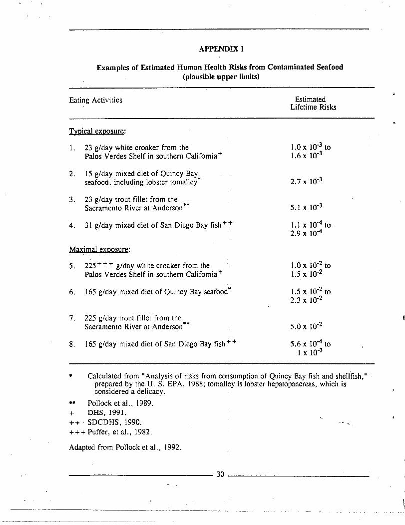
APPENDIX I

Examples of Estimated Human Health Risks from Contaminated Seafood(plausible upper limits)

Eating Activities

Typical exposure:

1. 23 g/day white croaker from thePalos Verdes Shelf in southern California+

2. 15 g/day mixed diet of Quincy Bayseafood. including lobster tomalleY*

3. 23 g/day trout fillet from theSacramento River at Anderson**

4. 31 g/day mixed diet of San Diego Bay fish ++

Maximal eXQOsure:

5. 225 ++ + g/day white croaker from thePalos Verdes Shelf in southern California+

6. 165 g/day mixed diet of Quincy Bay seafood'"

7. 225 g/day trout fillet from the **Sacramento River at Anderson

8. 165 g/day mixed diet of San Diego Bay fish + +

EstimatedLifetime Risks

1.0 x 10-3 to1.6 x 10-3

2.7 x 10-3

5.1 x 10-3

1.1 X 10-4 to·2.9 x 10-4

1.0 x 10-2 to1.5 x 10-2

1.5 x 10-2 to2.3 x 10-2

5.0 x 10-2

5.6 X 10-4 to1 x 10-3

• Calculated from II Analysis of risks from consumption of Quincy Bay fish and shellfish," .prepared by the U. S. EPA, 1988; tomalley is lobster hepatopancreas, which isconsidered a delicacy. ;;.

•• Pollock et al., 1989.+ DHS, 1991.++ SDCDHS, 1990.+++ Puffer, et al., 1982.

Adapted from Pollock et al., 1992.

---------------30 _

-------------------_._•.._ _ -

APPENDIX 2: List of Priority Pollutants and 301 (h) Pesticides Listed According to Structural Compound Class andOctanol/Water Partition Coefficients

Structural Compound Structural CompoundClass ppll Pollutant LogKow Class ppll Pollutant LogKow

Phenols 65 phenol 1.46 High Mol~ular Weight 39 fluoranthene 5.5334 2,4-dimethylphenol 2.42 Polynuclear Aromatic 72 benzo(a)anthracene 5.61

Hydrocarbons (PAH) 73 benzo(a)pyrene 6.00Substituted Phenols 21 2,4,6-trichlorophenol 3.69 74 benzo(b)fluoranlhene 6.60

22 para-chloro-mela-cresol 3.1.0 75 benzo(k)fluoranthene 6.8524 2-chlorophenol 2.16 76 chrysene 5.6031 2,4-dichlorophenol 3.08 79 benzo(ghi)perylene 7.0057 2-nilrophenol 1.77 82 dibenzo(a,h)anthracene 6.0058 4-nitrophenol 2.9 I 83 indeno (J .2,3-cd)pyrene 7.7059 2.4-dinitrophenol 1.53 84 pyrene 4.8860 4.6-dinitro-o-cresol 2.85

I 64 pentachlorophenol 5.00 Chlorinated Aromatic 8 1.2,4-trichlorobenzene 4.23wJ-' Hydrocarbons 9 hexachlorobenzene 5.23I

Organonitrogen 5 benzidine 1.81 20 2-ehloronaphthalene 4.72Compounds 28 3.3'-dichlorobenzidine 3.02 25 1.2-dichlorobenzene 3.40

35 2,4-dinitrotoluene 2.00 26 1.3-dichlorobenzene 3.4436 2,6-dinitrotoluene 2.00 27 1.4-dichlorobenzene 3.5337 1.2-diphenylhydrazine 2.9456 nitrobenzene 1.83 Chlorinated Aliphatic 52 hexachlorobutadiene 4.2861 N-nitrosodimethylamine -.58 Hydrocarbons 12 hexachloroethane 3.9362 N-nitrosodiphenylamine 3.13 53 hexachlorocyclopentadiene 5.5163 N-nitrosodipropylamine 1.31

Halogenated Ethers 18 bis(2-ehloroethyl)ether 1.12Low Mol~ularWeight I acenaphthene 3.92 40 4-ehlorophenyl ether 4.92Polynuclear Aromatic 55 naphthalene 3.59 41 4-bromophenyl ether 5.08Hydrocarbons (PAH) 77 acenaphthlene 4.08 42 bis(2-ehloroisopropyl)ether 2.58

78 anthracene 4.34 43 bis(2-ehloroethoxy)methane 1.2681 phenanthrene 4.4680 fluorene 4.38

I

app: Priority Pollutant designation numberbChlorinated 301 (hI pesticides that are not on the Prio!ity Pollutant lisl.COrganophosphorus 301 (hI pesticides that are not on the Priority Pollutant list.dNA = Not Applicabla

Adaplt:d from Tetra T~h. 1985.

(colltillued)

Structural CompoundClass ppll Pollutant LogKow

Structural CompoundClass ppll Pollutant LogKow

Phthalates 66 bis(2-ethylhexyl)phthalate 4.20 Pesticides (conl'd) 102 a-hexachlorocyclohexane 3.85}. 67 butyl benzyl phthalate 4.05 103 p-hexachlorocyclohexane 3.85

68 di-ll-butyl phthalate 5.15 104 o-hexachlorocyclohexane 3.8569 di-n-octyl phthalate 9.20 105 y-hexachlorocyclohexane 3.85

I 70 diethyl phthalate 1.40 113 toxaphene 3.30t,

71 dimethyl phthalate 1.61 mirexb 6.89methoxychlorb 4.30

Polychlorinated 106 PCB-1242 6.00 h' c 3.81" parat IonBiphenyls (PCB) 107 PCB-I 254 6.48 malathionc 2.89as Aroclors 108 PCB-1221 4.00 guthionc 2.18

109 PCB-1232 4.48 demetonC 1.93110 PCB-1248 6.11III PCB-1260 6.91 Volatile Halogenated 6 tetrachloromethane 2.64

I 112 PCB-1016 5.88 Alkanes 10 I ;2-dichloroethane 1.45l..J

11 I. I. I-trichloroethane 2.47NI Miscellaneous 129 TCDD (dioxin) 6.10 13 I.I-dichloroethane 1.78

Oxgenated 54 isophorone 1.67 14 1.1.2-trichloroethane 2.18Compounds 15 1.1.2.2-tetrachloroethane 2.39

16 chloroethane 1.54Pesticides 89 aldrin 3.00 23 chloroform 1.90

90 dieldrin 5.48 32 1.2-dichloropropane 2.2891 chlordane 6.00 44 dichloromethane 1.3092 DDT 5.75 45 chloromethane 0.9093 DOE 5.69 46 bromomethane 1.0094 DOD 6.00 47 bromoform 2.3095 a-endosulfan 3.60 48 dichlorobromoethane 1.8896 b-endosulfan 3.60 49 fluorotrichloromethane 3.5397 endosulfan sulfate 3.60 50 dichlorodifluromethane 2.1698 endrin 4.56 51 chlorodibromomethane -2.0899 endrin aldehyde 5.60100 heptachlor 5.45101 heptachlor epoxide 5.40

I

epp: Priority Poilutent designetion numberbChlorineted 301 thl pesticides thet ere not on the Priority Pollutent list.COrgenophosphorus 301 (hI pesticides thet ere not on the Priority Pollutant list.dNA = Not Applicable

Adapted from Tetra Tech, 1985.

_'.1 "

i~.':~i'illued)

Structural Compound . Structural CompoundClass ppa Pollutant LogKow Class ppa Pollutant LogKow

Volatile Halogenated 29 I,I-dichloroethylene 1.48 124 nickel NAd

Alkenes 30 1,2-tralls-dichloroethylene 1.97 125 selenium NAd

33 trails-I, 3-dichloropropene 1.98 126 silver NAd

33 cis-I,3-dichloropropene 1.98 127 thallium NAd

85 tetrachloroethene 2.88 128 zinc NAd

87 trichloroethene 2.4288 vinyl chloride 0.60 Miscellaneous 121 cyanide NAd

116 asbestos NAd

Volatile Aromatic 4 benzene 2.11Hydrocarbons 38 ethylbenzene 3.15

86 toluene 2.21

Volatile Chlorinated 7 chlorobenzene 3.79

I Aromatic HydrocarbonswwI Volatile Unsaturated 2 acrolein 0.90

Carbonyl Compounds 3 acrylonitrile 1.20

Volatile Ethers 19 2-chlorethylvinylether 1.28bis(chloromethyl)ether

Metals 114 antimony NAd

115 arsenic NAd

117 beryllium NAd

118 cadmium NAd

119 chromium III NAd

119 chromium VI NAd

120 copper NAd

122 lead NAd

123 mercury NAd

123 methylmercury NAd

123 phenylmercury NAd

Metals (cont',U) 123 mercuric acetate NAd

I

app: Priority Pollutnnt dosionation numbor .bChlorinated 301 (h) pesticides thet are not on tha Priori tv Pollutant list.COrganophosphorus 301 (h) pasticides that ara not on tha Priority Pollutant list.dNA = Not Applicable

Adaptt:d from Tt:lra Tech, 1985.

A P PEN 0 I X E

Staff Report by the Division of Water QualityCriteria to Rank To~ic Hot Spots-in

Enclosed Bays and Estuaries of California

This report is provided for information only. This staff report:will berevised and the various issues discussed in the staff report will be includedin a draft Functional Equivalent Document for amendments to the CaliforniaEnclosed Bays and Estuaries Plan.

SlAlE Of CAlIfOR~IA

STATE ~AT[R RESOURCES CO~TROl BOARDDIVISIO~ Of ~ATER QUALITY

Staff Report:

CRITERIA TO RA~K TOXIC HOT SPOTS I~ E~ClOSED

BAYS A~D ESTUARIES OF CALIFOR~IA

March 1993

DRAFT

•

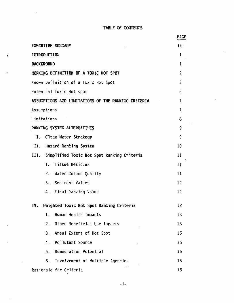
TABLE Of CO~TE~TS

EXECUTIVE S~V

X~TROOUCnOOI

8AC!(GROU~D

WOROCI~G DEFI~XTIOOO Of A TOXIC HOT SPOT

Known Definition of a Toxic Hot Spot

Potential Toxic Hot spot

ASSUMPTiOOOS A~O lIMITATIO~S Of THE RA~OCI~G CRITERIA

Assumptions

Limitat ions

RA~OCI~G SVST~ AlTER~TIVES

I. Clean ~ater Strategy

II. Hazard Ranking System

III. Simplified To~ic Hot Spot Ranking Criteria

1. Tissue Residues

2. Water Column Quality

3. Sediment Values

4. Final Ranking Value

IV. ~eighted lo~ic Hot Spot Ranking Criteria

1. Human Health Impacts

2. Other Beneficial Use Impacts

3. Areal Extent of Hot Spot

4. Pollutant Source

5. Remediation Potential

6. Involvement of Multiple Agenciesf:'

Rationale for Criteria

-i-

PAGE

iii

1

1

2

3

6

7

7

8

9

9

10

11

II

11

12

12

12

13

13

15

15

15

15

15

PAGE

STAFF RECOMMENDATION 21

TRIAL APPLICATION OF THE RANKING CRITERIA 21

RANKING OF POTENTIAL HOT SPOTS 24i

REFERENCES 25 i.

APPENDIX 1 THE CLEAN WATER STRATEGY 28

APPENDIX 2 HAZARD RANKING SYSTEM 44

APPENDIX 3 CHEMICAL SPECIFIC VALUES USED FOR 48HOT SPOT RANKING SYSTEM

-ii-

,

EXEcurI~E S~Y

California Water Code Section 13393.5 requires the State Water Board to adoptcriteria for the priority ranking of toxic hot spots in bays and estuaries.The criteria are to take into consideration factors relating to public health,environmental quality, toxic hazards to fish, shellfish, and wildlife, and theextent to which deferral of remedial action is likely to result in increases inhuman health risks, environmental damage or cleanup costs. The priorityranking of toxic hot spots for each region is to be included in a Toxic HotSpot Cleanup Plan which describes a number of factors including identificationof likely sources of the pollutants that are creating the toxic characteristicsat the site and actions to be taken to remediate each site. Waste dischargerequirements for each source identified as contributing to a toxic hot spot areto be reviewed and revised (with certain exceptions) to prevent furtherpollution of existing toxic hot spots or the creation of new hot spots. Thereevaluation ofpermits is to be conducted in the order established by the priority ranking ofknown tox ic hot spots. '

Staff has reviewed two ranking systems potentially suitable for satisfying theWater Code Section 13393.5 requirements: the State Water Board's Clean WaterStrategy and the U.S. Environmental Protection Agency's Hazard Ranking System.Since these systems were developed for purposes other than ranking of toxic hotspots for Bay Protection and Toxic Cleanup Program (BPTep), they cannot bedirectly applied to the program. Staff has developed two alternative systemsfor State Water Board consideration.

The principal characteristics of the alternatives are that they are based onthe definition of a toxic hot spot and rely only on existing information todevelop the rankings. The principal difference between the two alternatives isthe degree of detail provided in the rankings. The recommended alternative(which is a modification of Clean Water Strategy) utilizes all available,relevant information whereas the other alternative uses only some pertinentinformation. The ranking system is designed to be integrated with monitoringbeing conducted under the BPTep. The monitoring data and other pertinentinformation will be used in establishing site rankings.

This report contains an overview of the statutory and programmaticconsiderations relevant to the development of ranking criteria. A briefdescription of the Clean Water Strategy and the Hazard Ranking System isprovided, followed by the two alternative systems developed by staff. Therecommended alternative and an illustration of its application are alsopresented. Further details on each of the ranking systems are provided in theappendices.

- iii-

CRITERIA TO RANOC TOXIC HOT SPOTS I~

E~ClOSED BAVS A~D ESTUARIES Of CAlIFaR~IA

I~TRODUCTIO~

The development of criteria for the priority ranking of toxic hot spots inenclosed bays and estuaries is required by statute. This report reviews thestatutory requirements, programmatic considerations, various ranking systems,and presents a recommended system for use in the Bay Protection and ToxicCleanup Program (BPTCP). Appendices are included which provide detail on theranking systems reviewed and numeric values for use in the recommended system.

Four alternative ranking systems are reviewed in this staff report. Theseinclude the two existing ranking systems, the State Water Board's Clean WaterStrategy and the U.S. Environmental Protection Agency's Hazard Ranking Systemused for ranking Superfund sites. Two additional ranking systems developedspecifically to address programmatic considerations of the BPTCP are presented.One of these, a modification of the Clean Water Strategy, is proposed for useby the BPTCP.

The site ranking criteria proposals were first discussed at the January 7, 1993State Water Board Workshop. At that workshop, the State Water Board directedthe staff to conduct a staff workshop to solicit public comment. Staffworkshops were held on January 26 and 28, 1993. This staff report and theproposed ranking criteria have been revised as a result of the commentsreceived on this subject.

The working definition of a toxic hot spot is presented below to provide thecontext for recommending site ranking criteria. The State Water Board staff donot recommend the adoption of this definition at this time. The State andRegional Water Board staff would like to gain additional experience with thisdefinition before it is adopted by the State Water Board. After thisdefinition is tested more fully, we will bring the definition before the StateWater Board for consideration as a Statewide plan amendment or forconsideration for adoption by resolution. The ranking criteria proposed inthis staff report will be useable with any definition of a toxic hot spot.

BACOCGROUND

The BPTCP is a comprehensive effort to regulate toxic pollutants in enclosedbays and estuaries of the State. The program consists of both short-term andlong-term activities. The short-term activities include the identification andpriority ranking of toxic hot spots, development and implementation of regionalmonitoring programs designed to identify toxic hot spots, development ofnarrative sediment quality objectives, development and implementation ofcleanup plans, revision of waste discharge requirements as needed to alleviateimpacts of toxic pollutants, and development of a comprehensive databasecontaining informatiori pertinent to describing and managing toxic hot spots.The long-term activities include development of numeric sediment qualityobjectives; development and implementation of strategies to prevent theformation of new toxic hot spots and to reduce the severity of effects from

-1-

existing toxic hot spots; reV1Slon of water quality control plans, cleanupplans, and monitoring programs; and maintenance of the comprehensive database.The California Water Code, Section 13393.5, requires the State Water Board todevelop and adopt criteria for the priority ranking of toxic hot spots inenclosed bays and estuaries. The criteria are to IItake into account pertinentfactors relating to public health and environmental quality, including but notlimited to potential hazards to public health, toxic hazards to fish,shellfish, and wildlife, and the extent to which the deferral of a remedialaction will result or is likely to result in a significant increase inenvironmental damage, health risks or cleanup costs. 1I

The role of the ranking criteria is to provide a prioritized list of sitesbased on the severity of the identified problem. The Water Code calls forwaste discharge requirements to be reevaluated in the ranked order. Water CodeSection 13395 states, in part, that the Regional Boards shall lIinitiate areevaluation of waste discharge requirements for dischargers who, based on thedetermination of the Regional Board, have discharged all or part of thepollutants which have caused the toxic hot spot. These reevaluations shall befor the purpose of ensuring compliance with water quality control plans andwater quality control plan amendments. These reevaluations shall be initiatedaccording to the priority ranking established pursuant to subdivision (a) ofSection 13394 and shall be initiated within 120 days from, and the last shallbe initiated within one year from, the ranking of toxic hot spots. 1I

The priority ranking for each site is to be included in a Toxic Hot SpotCleanup Plan which describes a number of factors including identification oflikely sources of the pollutants that are causing the toxic characteristics andactions to be taken to remediate each site. The regional list of ranked hotspots will be consolidated into a statewide prioritized list of toxic hotspots, and included in the statewide Toxic Hot Spot Cleanup Plan.

Within specificed periods of time, waste discharge requirements for each sourceidentified as contributing to a toxic hot spot are to be reviewed.and revised(with certain exceptions) to prevent further pollution of existing toxic hotspots or the formation of new hot spots. The reevaluation of permits is to beconducted in the order established by the priority ranking of hot spots.

WOR~ING DEFINITION OF A TOXIC HOT SPOT

Water Code Section 13391.5 defines toxic hot spots as "... locations in enclosedbays, estuaries, or any adjacent waters in the 'contiguous zone' or the'ocean' ... the pollution or contamination of which affects the interests of thestate, and where hazardous substances have accumulated in the water or sedimentto levels which (1) may pose a substantial present or potential hazard toaquatic life, wildlife, fisheries, or human health, or (2) may adversely affectthe beneficial uses of the bay, estuary, or ocean waters as defined in waterquality control plans, or (3) exceeds adopted water quality or sediment qualityobjectives. II

While the statutory definition provides the basis for identifying hot spots,practical implementation requires a more detailed definition. Accordingly, theBPTCP has developed a working definition that includes five "triggers" fordetermination of a known toxic hot spot:

-2-

Known Toxic Hot Spot

A site meeting anyone or more of the following conditions is considered to bea known toxic hot spot:

1. Site exceeds water or sediment quality objectives for toxic pollutants thatare contained in appropriate water quality control plans.

This finding requires chemical measurement of water or sediment, ormeasurement of toxicity using tests and objectives stipulated in waterquality control plans. Determination of a toxic hot spot employing thisfinding should rely on recurrent measures over time (at least separatesampling dates). Suitable time intervals between measurements must bedetermined by staff.

2. Water or sediment exhibits toxicity associated with toxic pollutants, basedon confirmatory toxicity tests acceptable to the BPTCP.

To determine whether toxicity exists, recurrent measures (at least 2separate sampling dates) should demonstrate an effect. Appropriatereference and control measures must be included in the toxicity testing.The methods acceptable to and used by the BPTCP may include some toxicitytest protocols not referenced in water quality control plans (Table 1).Toxic pollutants should be present in the media at concentrations sufficientto cause or contribute to toxic responses in order to satisfy thiscondition.

3. Tissue toxic pollutant levels of organisms collected from the site exceedlevels established by the Office of Environmental Health Hazard Assessment(OEHHA), California Department of Health Services (DHS), United States Foodand Drug Administration (FDA) for the protection of human health, or theNational Academy of Sciences (NAS) for the protection of human health orwildlife, or a health warning against the consumption of such organisms hasbeen issued by OEHHA or DHS.

Acceptable tissue concentrations are measured either as muscle tissue(preferred) or whole body residues. Residues in liver tissue alone are notconsidered a suitable measure for known toxic hot spot designation. Animalscan either be deployed (if a resident species) or collected from residentpopulations. Recurrent measurements are required. Residue levelsestablished for the protection of human health can be applied to anyconsumable species.

Shellfish: Except for existing information, each sampling episode shouldinclude a minimum of three replicates and the value of interest is theaverage value of the replicates. Each replicate should be comprised of atleast 15 individuals. For existing State Mussel Watch information relatedto organic pollutants, a single composite (20-100 individuals) sample may beused instead of the replicate measures. When recurrent measurements exceedone of the levels referred to above, the site is considered a known toxichot spot.

-3-

Fin-fish: A mlnlmum of three replicates is necessary. The number ofindividuals needed will depend on the size and availability of the animalscollected; however, a minimum of five animals per replicate is recommended.The value of interest is the average of the three replicates. Animals ofsimilar age and reproductive state should be used.

4. Impairment is associated with toxic pollutants found in residentindividuals.

Impairment means reduction in growth, reduction in reproductive capacity,abnormal development, histopathological abnormalities, or identification ofadverse effects using biomarkers. Each of these measures must·be made incomparison to a reference condition (the endpoint measured in the samespecies and tissue collected from an unpolluted site).

Growth Measures: Reductions in growth can be addressed using suitablebioassays acceptable to the BPTep (Table 1) or through measurements of fieldpopulations.

Reproductive Measures: Reproductive measures must clearly indicatereductions in viability of eggs or offspring, or reductions in fecundity.Suitable measures include pollutant concentrations in tissue, sediment, orwater which have been demonstrated in laboratory tests to cause reproductiveimpairment; significant differences in viability or development of eggsbetween reference and test sites; differences in sex ratios sufficient todecrease reproductive success.

Abnormal Development: Abnormal development can be determined using measuresof physical or behavioral disorders or aberrations. Indications that thedisorder can be caused by toxic pollutants, in whole or in part, must beavailable.

Histopathology: Abnormalities representing distinct adverse effects, suchas carcinomas or tissue necrosis, must be evident. Indications that toxicpollutants are capable of causing or contributing to the disease conditionmust also be available.

Biomarkers: Direct measures of physiological disruption or biochemicalmeasures representing adverse effects, such as significant DNA strandbreakage or perturbation of hormonal balance, must be evident. Biochemicalmeasures of exposure to pollutants, such as induction of stress enzymes, arenot by themselves suitable for determination of known toxic hot spots.Indications that a toxic pollutant causes or contributes to the adverseeffect are needed.

5. Significant degradation in biological populations and/or communitiesassociated with the presence of elevated levels of toxic pollutants.

This condition requires a demonstration that diminished numbers of speciesor changes in the number of individuals of a single species (when comparedto a reference site) are associated with concentrations of toxic pollutants.The analysis should rely on measurements from multiple stations. Careshould be taken to ensure that at least one site is not degraded so that asuitable comparison can be completed.

-4-

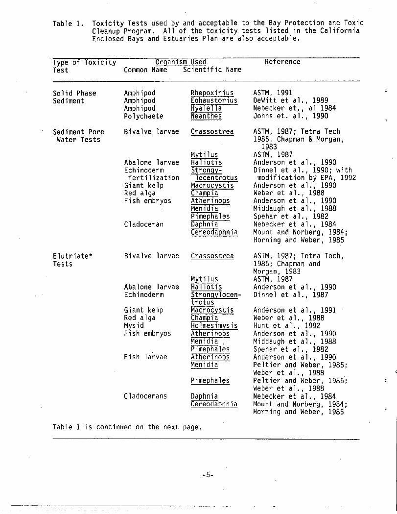
Table 1. Toxicity Tests used by and acceptable to the Bay Protection and ToxicCleanup Program. All of the toxicity tests listed in the CaliforniaEnclosed Bays and Estuaries Plan are also acceptable.

Type of ToxicityTest

Organism UsedCommon Name Scientific Name

Reference

Solid PhaseSediment

Sediment PoreWater Tests

Elutriate*Tests

AmphipodAmphipodAmphipodPolychaete

Bivalve larvae

Abalone larvaeEchinodermfertilization

Giant kelpRed (llgaFish embryos

Cladoceran

Bivalve larvae

Abalone larvaeEchinoderm

Giant kelpRed algaMysidFish embryos

Fish larvae

Cladocerans

Rhe oxin.iusEo austorlUSHyalellaNeanthes

Crassostrea

Myt il usHaliotisStrongy-

locentrotusMacrocystisChampiaAtherinopsMenidiapimephalesDaphniaCereodaphnia

Crassostrea

MytilusHaliotisStrongylocen­trotusMacrocystisChampiaHolmesimysisAtherinopsMenidia ,PimephalesAtherinopsMenidia

Pimephales

DaphniaCereodaphnia

ASTM, 1991DeWitt et al., 1989Nebecker et., al 1984Johns et. al., 1990

ASTM, 1987; Tetra Tech1986, Chapman &Morgan,

1983ASTM, 1987Anderson et al., 1990Dinnel et al., 1990; withmodification by EPA, 1992

Anderson et al., 1990Weber et al., 1988Anderson et al., 1990Middaugh et al., 1988Spehar et al., 1982Nebecker et al., 1984Mount and Norberg, 1984;Horning and Weber, 1985

ASTM, 1987; Tetra Tech,1986; Chapman andMorgan, 1983ASTM, 1987Anderson et al., 1990Dinnel et al., 1987

Anderson et al., 1991Weber et al., 1988Hunt et al., 1992Anderson et al., 1990Middaugh et al., 1988Spehar et al., 1982Anderson et al., 1990Peltier and Weber, 1985;Weber et al., 1988Peltier and Weber, 1985~Weber et al., 1988Nebecker et al., 1984Mount and Norberg, 1984;Horning and Weber, 1985

Table 1 is continued on the next page.

-5-

Table 1 (continued)

Type of Toxicity Organism UsedTest Common Name Scientific Name

Reference

Ambient Water Bivalve larvae

Abalone larvaeEchinodermfertilization

Giant kelpRed algaMysidFish embryos

Fish larvae

Cladocerans

Crassostrea

HaliotisStrongylocen­trotus

MacrocystisChampiaHolmesimysisAtherinopsMenidiaPimephalesAtherinopsMenidia

Pimephales

DaphniaCereodaphnia

ASTM, 1987; Tetra Tech,1986; Chapman andMorgan, 1983Anderson et al., 1990Dinnel et al., 1987;with modifications byEPA, 1992Anderson et al., 1991Weber et al., 1988Hunt et al., 1992Anderson et al., 1990Middaugh et al., 1988Spehar et al., 1982Anderson et al., 1990Peltier and Weber, 1985Weber et al., 1988Peltier and Weber, 1985Weber et al., 1988Nebecker et al., 1984Mount and Norberg, 1984Horning and Weber, 1985

* Elutriate toxicity tests are of value in estimating the toxicity ofdisposed sediments to aquatic organisms. Elutriate test results can beused to qualify a site as a potential hot spot but should not be usedto confirm a site as a known hot spot. Either a pore water or a solidphase test should be used to confirm toxicity.

Sites are designated as known hot spots after generating information whichsatisfies anyone of the five conditions of the working definition. Toutilize this working definition, a list of toxicity tests has beenassembled. This list identifies toxicity tests that can be employed inmonitoring and surveillance activities described in regional monitoringplans and partially satisfies the Water Code requirement [Section13392.5(a)(2)] for standardized analytical methods (Department of Fish andGame Marine Pollutant Studies Laboratory, 1992). The BPTCP toxicity methodsare listed in Table 1.

Potential Toxic Hot Spot

In addition to the identification of known toxic hot spots the statuterequires the identification of suspected or potential hot spots (Water CodeSection 13392.5). Sites with existing information indicating a possibilityof impairment but without sufficient information to allow a findingconsistent with the working definition of a known toxic hot spot areclassified as potential hot spots. More specifically, four conditionssufficient to identify a potential hot spot have been determined. If anyone of these conditions is satisfied a site can be designated a potentialtoxic hot spot. These are:

-6-

1. Concentrations of toxic pollutants are elevated above background levelsbut insufficient data are available on the impacts associated with suchpollutant levels to determine the existence of a known toxic hot spot;

2. Water or sediments containing toxic pollutants exhibit toxicity inscreening tests or tests other than those used by the BPTCP;

3. Tissue toxic pollutant levels in resident or test species are elevatedbut do not meet conditions for determination of the site as a known hotspot; tissue toxic pollutant levels exceed Maximum Tissue Residue levels(MTRLS) derived from water quality objectives contained in appropriatewater quality control plans; or a health warning has been issued for thesite by a local public health agency; and/or

4. The level of pollutant at a site exceeds Clean Water Act, Section 304(a)criterion, or sediment quality guidelines or EPA sediment toxicitycriteria for toxic pollutants.

ASSUMPTIONS AND LIMITATIONS OF THE RANKING CRITERIA

The Water Code Section 13393.5 requires that the criteria take intq account"pertinent factors relating to public health and environmental quality,including but not limited to, potential hazards to public health, toxic hazardsto fish, shellfish, and wildlife, and the extent to which the deferral of aremedial action will result or is likely to result in a significant increase inenvironmental damage, health risks or cleanup costs."

In addition to the considerations stipulated in Water Code Section 13393.5,several assumptions were applied to the evaluation of the various alternativeranking systems.

Assumptions

1. Criteria should address broad programmatic priorities.

2. Criteria are to be used to organize internal work and program activities(i.e., the evaluation of the need to adjust permit limits or monitoringpriorities).

3. Criteria are not designed to determine regulatory enforcement actions.

4. Ranking should be based on existing information at the time of ranking;additional studies should not be required for the purpose of prioritizingknown or potential toxic hot spots (potential toxic hot spots ~ill beidentified and additional information will be needed before a potentialsite can be ranked as a known toxic hot spot).

5. Assessment of cost and feasibility of remedial actions for a site will beconsidered in toxic hot spot cleanup plans but factors that influence costwill be considered.

6. The priority list will be revised periodically.

-7-

v

7. All other factors being equal, sites that are well characterized (i.e.,significant amounts of available data) will rank higher than sites that areless well characterized (i.e., few available data and greater uncertaintyabout the site).

~

1 8. The best available scientific information will be used to evaluate the dataavailable for site ranking.

9. Sites for which cleanup or remediation has been implement~d but whichretain toxic hot spot characteristics will only be considered for rerankingif circumstances change that would allow for further reducing adverseimpacts at the site. A list of sites that have been remediated withoutcomplete removal of toxic hot spot characteristics will be maintained.

10. A site that has been remediated will be removed from the priority list.

Li~itations

The ranking criteria are intended to provide the relative priority of a sitewithin the group of sites considered to be known toxic hot spots. Since notall sites will have the same scope and quality of information available at thetime of ranking, this relative placement should be founded in measures of thepotential for adverse impacts. The determination that some adverse impacts areoccurring at the sites will have been made previously to the ranking and inaccordance with the definition of a toxic hot spot. While the ranking shouldreflect the severity of the demonstrated adverse impacts, the full scope ofecological and human health impacts will likely not be characterized at thetime of ranking, and therefore, should not be the goal of the ran~ing criteria.These impacts may be addressed as part of the activities conducted pursuant tothe cleanup plans. The ranking criteria should provide a mechanism todiscriminate among all those sites considered to be toxic hot spots (using thewater code definition or other more specific definition) and thereby providefor a placement of each site relative to other sites under consideration.

The ranking criteria are not to be used to define a toxic hot spot. Thedetermination of whether a site qualifies to be considered a toxic hot spot isa separate and previous step. The BPTCP has establised a detailed workingdefinition of a toxic hot spot, which is consistent with the statutorydefinition contained in Water Code Section 13391.5. The working definitionpresented above is not proposed for adoption by the State Water Board at thistime.

The ranking criteria are not to be used to define cleanup actions or establishcleanup levels. The actions to be undertaken to cleanup or remediate a sitewill be developed on a case-by-case basis for each site. The considerations tobe addressed at all sites, together with special considerations for each site,will be described in the cleanup plans required by Water Code Section 13394.

-8-

RANKING SYSTEM ALTERNATIVES

Four ranking systems are presented for consideration. Two of these systemswere developed for purposes somewhat different than those of the BPTCP. Theseare the Clean Water Strategy used by the State Water Board for resourceallocations, and the Hazard Ranking System used by US EPA for Superfund siteprioritization. These systems are offered for consideration because they areestablished and have been used with success for their respective purposes.

I. Clean Water Strategy

The State Water Board1s Water Quality Coordinating Committee, in 1990,has developed the Clean Water Strategy (Strategy) as a management tool toprovide a common framework for applying the collective professionaljudgement of State and Regional Water Board staff to identify andprioritize water quality problems (Diaz, 1991). The Strategy consists ofsix phases which, to date, have been partially implemented. These phasesare: (1) collecting water quality information, (2) comparing and rankingthe importance and the condition of water bodies, (3) prioritizing workrequired to address threats and impairments of water quality identifiedin Phase 1, (4) allocation of staff and contract resources to the listgenerated in Phase 3, (5) implementation of the funded work, and (6)review and assessment of results and products. CWS rankings aredeveloped through a collective professional judgement process. Thisprocess uses criteria and numerical ratings to allow statewide staff toseparate and group waters in five levels of importance (value of theresource) and within each each level of importance, to group the severityof problems in five levels. The CWS does not rely on formulas orweighted criteria in developing rankings. The CWS process relies on aseries of IIbite size 'l judgements an d groupings, which when combinedresult in general concensus on final r~nkings.

Phases 1 and 2 of the Strategy might be applied to satisfy the Water Coderequirements for Toxic Hot Spot ranking in the BPTCP. While the basicpurpose of the Strategy is to prioritize responses to water qualityproblems (similar to Toxic Hot Spot ranking) there are some fundamentaldifferences in purpose and approach between the Strategy and therequirements of the BPTCP. The most fundamental difference is that theStrategy creates priorities for work based on ranking of entire waterbodies whereas the Hot Spot Ranking is intended to address hot spotswhich, except in extraordinary cases, are likely to be localized areas.In addition, the Strategy must consider a number of water qualityimpairments other than those caused by toxic pollutants. For instance,depressed levels of dissolved oxygen should be considered in the Strategybut would be excluded for BPTCP purposes. A third difference is that theStrategy generates independent ranked lists for several classes of waterbodies (such as rivers, lakes, and wetlands), while the BPTCP is requiredto rank hot spots together, irrespective of the type of water body (suchas wetlands; fresh, brackish, and marine portions of estuaries; andbays). Finally, the Strategy rankings are designed to support Phases 3and 4; i.e., proposed responsive actions and allocation of resources. Inthe BPTCP, determination of likely responsive actions to hot spotdesignations are included as part of Toxic Hot Spot Cleanup Plans and arenot included in the ranking process.

-9-

Since the Strategy was developed before the BPTCP was established, itwill likely be modified to incorporate new information from the BPTCP. Alikely outcome of this modification will be that the toxic hot spotrankings will be included as one of the many factors used to developwater body rankings in the Strategy. In any case, the Strategy willcontinue to be used for purposes beyond the scope of the BPTCP. Asummary of the ranking process using the Strategy is provided inAppendix 1.

II. Hazard Ran~ing System

The Hazard Ranking System (HRS) was developed as part of theimplementation of the national Superfund program (US EPA, 1990). The HRSis designed to score the relative threat associated with actual orpotential releases of hazardous substances from specific sites and torank the site on the National Priority List for superfund cleanup. TheHRS provides a numerical value derived from the assessment of fourdifferent environmental pathways each evaluated for three specificfactors. The pathways are: (1) ground water migration, (2) surfacewater migration, (3) soil exposure, and (4) air migration. The threefactors are (1) the likelihood of release, (2) waste characteristics, and(3) targets. Through a series of steps, each pathway is assigned anumerical score which integrates the assessment of the three factors forthat pathway. The pathway scores are then combined to produce the finalsite value. The site is ranked against other sites based on this finalsite value; larger numeric values receive a higher priority.

The actual derivation of a final site value is a rather complex processthat requires a significant amount of site-specific information. Somesteps in the process are common to all four pathways while others arespecific to the particular pathway under consideration.

While the HRS provides a somewhat consistent treatment of sites forranking purposes, the requirement of extensive evaluation makes it rathercumbersome and time consuming process. Furthermore, this system stillrequires a number of assumptions and professional judgement in order tocomplete the evaluation and ranking. The HRS was developed underguidance from Congress that the system "to the maximum extent feasible,.. accurately assesses the relative degree of risk to human health andthe environment posed by sites and facilities subject to review" (Fed.Reg. Vol 55, No. 241, pg 51532). Although this directive does notconstitute a mandate for a full risk assessment before ranking, it hasbeen interpreted to require a more detailed analysis (as evidenced by theHRS) than required for the purposes of the BPTCP. The level of detailsrequired to complete an HRS evaluation does not seem justified for BPTCPpurposes.

Furthermore, the HRS is designed to emphasize threats to human health.For example, two of the three factors in the surface water-overland/floodmigration path address human exposure (drinking water threat and humanfood chain threat), and one factor addresses environmental threats(sensitive environments). The scores for these factors further emphasizehuman health by allowing a maximum score for drinking water and foodchain factors of 100 but only a maximum of 60 for environmental threats.

-10-

When scores are computed for the final site value, the emphasis clearly fallson human health considerations. This is in contrast to the BPTCP where humanhealth and environmental (aquatic life and wildlife) considerations are givenequal weight. Appendix II provides further information on the HRS criteria.

III. Simplified Toxic Hot Spot Ranking Criteria

In looking for the simplest approach to ranking, it becomes clear thatusing a single type of information greatly reduces the complexity of theproblem. An approach using only chemical data is presented below. Thisapproach satisfies Water Code requirements. It is quite easy and simpleto use but loses detail in the rankings when compared to the weightedtoxic hot spot ranking criteria discussed subsequently in this report.

SIMPLIFIED RANKING CRITERIA

1. Tissue residues:

Assign values based on criteria listed below and using the averageconcentration of pollutants reported for any organisms collected from thesite for a single sampling event. Assign a value for each substance thatexceeds its MTRL. Select the substance providing the highest score.

If a concentration of a toxic substance in tissue:

Equals or exceeds MTRL1 of 1000 ug/kg assign a value of 1Between MTRL of 10 ug/kg and 1000 ug/kg assign a value of 2Less than or equal to MTRL of 10 ug/kg assign a value of 3

Multiply by 2 if more than one substance exceeds its MTRL in the samesample.

2. Water column quality:

Assign values based on criteria listed below and using the concentration ofpollutants reported for ambient waters collected from the site. Use thesubstance providing the highest score for exceeding water qualityobjectives in the appropriate statewide ;plan. Ranking values are assignedbased on the values below:

For water quality objective equal to or over 1 mg/l, assign a value of 1.

For water quality objective between 100 ug/l and 1 mg/l, assign a value of2.

For water quality objective less than 100 ug/l, assign a value of 3.

Multiply by 2 if more than one substance exceeds its applicable waterquality objective.

1 MTRLs (Maximum Tissue Residue Levels) are calculated by multiplying the'human health water quality objective in the appropriate statewide plan bythe chemical1s bioconcentration factor (BCF) (Cohen, 1993). The BCF isdefined as the ratio of the contaminant concentration in tissue tocontaminant concentration in water. MTRLs proposed for use in the rankingsystem are presented in Appendix 3.

-11-

3. Sediment values:

Assign values based on sediment weight-of-evidence guidelines recommendedfor the State of Florida and the criteria listed below and using the dryweight normalized concentration in bulk sediments collected from the site.Use the substance providing the highest score.

Above the Probable Effects Level (PEL) assign a value of 3.

Between the No Observed Effect Level (NOEL) and PEL assign a value of 2.

Multiply by 2 if more than one substance exceeds to NOEL.

4. Final Ranking Value:

Values should be generated for criteria 1 through 3 wherever possible. Insome cases it will not be possible to generate a criterion. For example, apollutant of concern may not have an associated sediment value. In thesecases assign a value of zero for each criterion that cannot be fullydeveloped.

Sum the values for criteria 1 through 3. The resulting sum is the finalranking value. The site with the highest score will be assigned rank #1.

IV. Weighted Toxic Hot Spot Ran~ing Criteria

The ranking system presented below has been designed to (1) provide asite-specific refinement of the Clean Water Strategy and (2) addressspecific requirements of the BPTCP (Water Code Sections 13390 et seq.).A value for each criterion described below should be developed providedappropriate information exists. Any criterion for which no informationexists should be assigned a value of zero. The sum of the values for thesix criteria will serve as the final ranking score. In developing thescore for each criterion an initial value is identified and then adjustedby one or two correction factors as appropriate.

-12-

dose

WEIGHTED RANKING CRITERIA

1. Human Health Impacts

Potential Exposure: Select from the following the applicable circumstancewith the highest value:

Human Health Advisory issued for consumption of aquatic life from the ~

site (assign a value of 5); Human Health advisory issued for sensitivepopulations consuming aquatic life from the site (4); Tissue residues inaquatic organisms exceed FDA/DHS action level or OEHHA trigger level (ifavailable for the location) (3); Tissue residues in aquatic organismsexceed MTRL (2).

Potential Hazard: Multiply the exposure value selected by one of thefollowing factors:

Pollutant(s) of concern is(are) known or suspected carcinogen2 with acancer potency factor or an other pollu.tant of concernwith a r~ferbce(assign a value of 5); Pollutant(s) of concern is(are) not known orsuspected carcinogens without a cancer potency factor or pollutant ofconcern without an RFD (3); other pollutants of concern (1).

2. Other Beneficial Use Impacts

A. Rare, threatened, or endangered species present: Select from thefollowing the applicable circumstance with the highest value and oneother value if applicable. Do not use any species twice:

Endangered species present at the site (assign a value of 5),Threatened or rare species regularly present at the site (4),Threatened or rare species occasionally present at the site (3).

Multiply each identified value by 2 if multiple species are present inany category. Add all resultant values for final Criteria 2A value.

2 These are substances suspected of being carcinogenic as classified in theEPA Integrated Risk Information System (IRIS), by the Office ofEnvironmental Health Hazard Assessment or by the Department of HealthServices. A list of the substances proposed for use in the ranking systemis provided in Appendix 3.

-13-

B.'Demonstrated aquatic life impacts: Select 'one or 'more 'V:alue('s,~:

Commun ity impa i rments assoc iated with tox ic pollutants (ass+gn C(3 lv'a"hteof 5), statistically significant toxicity demonstrate'd with:'a'cu'tetoxicity tests acceptable to the BPTCP (4), Statistically ~i~nific~nt,

toxicity demonstrated in chronic toxicity tests accepta'ble to the 'BPrCP(3), reproductive impairments documented '(2), toxicity is demonstratedon ly occas iona lly and does not appear s'evere enough to alter res identpopulations (1).

Multiply each value by 2 if the demonstrated effects exceed 80 percentof the organisms in any given test or 80 pecentof the species in theanalysis.

C. Chemical measures3:

i. Tissue residues exceed NAS guideline (assign a value of 3), at orabove State Mussel Watch Elevated Data Level (EDL) 95 (2), greaterthan State Mussel Watch EDL 85 but less than EDL 95 (1).

ii. Water quality objective: Exceeded regularly (assign a value of3), infrequently exceeded (2).

iii. Sediment values (sediment weight of evidence guidelinesrecommended for State of Florida)4: Above the Probable EffectsLeve1 5 (PEL) (3), between the NOEL6 and PEL (2). For asubstance with no calculated PEL: Above the effects rangemedian? (ER-M) (2), between the effects range lowest 10percent? (ER-L) and ER-M (1).

If multiple chemicals are above their respective EDL 85, water qualityobjective or sediment value, select the chemical with the highest valuefor each of the criteria (i) through (iii) above. Add the values for (i)through (iii) (above) to derive the initial value. Multiply the initialvalue by 2 if multiple chemicals are suspected of contributing to thetoxic hot spot.

3 The tissue residue guidelines and sediment values to be used in the rankingsystem should be the most recent version available. The guidelines andsediment values proposed for use in the ranking system are included inAppendix 3. Water quality objectives to be used are found in theCalifornia Enclosed Bays and Estuaries Plan, Inland Surface Waters Plan orCalifornia Ocean Plan (depending on which plan applies). Where a regionalwater quality control plan (Basin Plan) contains a more stringent valuethan the statewide plan. In such a case, the regional water qualityobjective will be used.

Footnotes 4, 5, 6 and 7 are listed on pages 20 and 21.

-14-

3. Areal Extent of Toxic Hot Spot

Select one of the following values:

More than 250 acres (assign a value of 10), 50 to 250 acres (B), 10 to lessthan 50 acres (6), less than 10 acres (4).

4. Pollutant Source

Select one of the following values:

Source of pollution identified (assign a value of 5), Source partiallyaccounted for (3), Source unknown (2), Source is an historic discharge andno longer active (1).

Multiply by 2 if multiple sources are identified.

5. Remediation Potential

Select one of the following values:

Site is unlikely to improve without intervention (4), site mayor may notimprove without intervention (2), site is likely to improve withoutintervention (1).

Multiply the selected value by one of the adjustment factors listed below:

Potential for immediate control of discharge contributing to the toxic hotspot or development of source control/waste minimization programs (assign avalue of 4), potential for implementation of an integrated preventionstrategy involving multiple dischargers (3), site suitable forimplementation of identified remediation methods (2). If site can not beclassified (assign a value of 1).

6. Involvement of multiple agencies

If government agencies other than the State or Regional Water Boards haveinterests in assessing or managing the site, assign a value of 10.

Rationale for Criteria

This section decribes the rationale for each of the six criteria listed above.

1. Human Health Impacts

The human health impacts criterion has two' parts: An estimate of potentialexposure and an estimate of potential hazard. For the exposure estimatethe highest score is given if a general human health advisory has beenissued. This type of advisory is an indication that aquatic life used forconsumption is severly contaminated (i.e., the beneficial use is severelyimpaired). A human health advisory issued for a sensitive population(e.g., pregnant women, subsistence fisherpersons, etc.) is less severe thanthe general advisory because fewer people would generally be affected. The

-15-

FDA/DHS action levels receive a lower score because these values do nottake into consideration the site-specific factors of the risk assesmentsused for human health advisory issued for a site. A tissue residue levelabove the MTRL does not by itself demonstrate a water body impairment.MTRLs receive the lowest scores because they are established for a specificconsumption rate (6.5 g/day for the Inland Surface Waters Plan and theEnclosed Bays and Estuaries Plan and 23 g/day for the California OceanPlan) and at a cancer risk level of one in one million.

The potential hazard factor assumes that the risk posed by known orsuspected carcinogens with a cancer potency developed or an other pollutantof concern with a reference dose available is greater than the risk posedby pollutants without a cancer potency or reference dose available. Thisis consistent with the approach taken in the three Statewide Plans, EPAmethods for calculating water quality criteria, and the approaches of OEHHAand DHS.

2. Other Beneficial Use Impacts

This criterion combines the various factors that should be considered inevaluating impacts on water quality, sediment quality, aquatic life andwildlife.

A. Rare, threatened or endangered species

This criterion evaluates the occurence of rare, threatened or endangeredspecies at a known toxic hot spot. The highest value is assigned if anendangered species is present and lower scores if threatened or rarespecies is regularly or occasionally present at the site. Association withendangered species is considered more severe than regular or occasionalpresence of rare or threatened species.

If multiple species in the categories are present the value is multipliedby 2. This value was selected to reflect the additional complexity of thesituation when more than one rare, threatened or endangered species ispresent.

B. Demonstrated Aquatic Life Impacts

This criterion is a measure of aquatic life impact from the most severeconditions to less severe conditions. Measurements of actual measuredmarine or bay community impairment indicates that there is a directmeasurement of impact. These kinds of impairments are difficult to measureand would only be measureable at the most highly impacted sites. Lowervalues are assigned to acute (short-term) and chronic toxicity (long-termor sensitive life stage tests) which serve as indicators of actual impacts.Reproductive impairements and occasional toxicity are given the lowestvalues because of the difficulty in interpreting these effects on aquaticlife populations.

If multiple species are effected the value is multiplied by 2 to reflect amore severe condition. This multiplier is also applied if over 80 percentof the test organisms are effected. This factor will allow fordistinctions to be made between moderate and more severe reponses oforganisms.

-16-

C. Chemical Measures

This criterion has three parts: (i) Tissue residues, (ii) water qualityobjectives, and (iii) sediment values. As described in the last section ofthis criterion, if multiple chemicals are suspected of contributing to theknown toxic hot spot then the sum of (i) through (iii) is multipled by "2".

i. Tissue Residues and Water Quality Objectives

Tissue residue levels are very difficult to evaluate in terms of impact onaquatic life but some measures do exist to aid in the interpretation ofchemicals bioaccumulated in fish or shellfish tissue. The NAS (1972) hasevaluated tissue residues for several chemicals. In this criterion, if an ~

NAS guideline is exceeded the highest score is received. Elevated datalevels (EDLs) from State Mussel Watch, are given lower values depending onwhether the EDL is above 95 percent or 85 percent. EDLs are given lowerscores because they do not measure actual effect on organisms. EDLs areincluded because State Mussel Watch information is generally available andthese data are valuable in assessing the relative exposure of organisms totoxic pollutants.

The "water quality objective" criterion gives a higher value when a waterquality objective from the appropriate ~ater quality control plan isexceeded regularly. If an objective is infrequently exceeded a lower scoreis given.

i;, Sediment Values

The inclusion of sediment values in evaluating chemical constituentconcentrations deserves some clarification. A major focus of the BayProtection statutes is the assessment of sediment quality. At this pointin time, a comprehensive collection of numeric values for toxic poll~tants

in sediment, similar to water quality objectives, does not exist. However,two related efforts have been completed that provide an overview ofsediment quality. These are the National Oceanic AtmosphericAdministration (NOAA) technical memorandum NOS OMA 52 by Long and Morgan(1990), and the sediment weight-of-evidence guidelines developed for theFlorida Coastal Management Program (1993).

Long and Morgan (1990) assembled data from throughout the country for whichchemical concentrations had been correlated with effects. These dataincluded spiked bioassay results and field data of matched biologicaleffects and chemistry. The product of the analysis is the identificationof two concentrations for each substance evaluated. One level, the EffectsRange-Low (ER-L) was set at the 10th percentile of the ranked data and wastaken to represent the point below which adverse effects are not expectedto occur. The second level, the Effects Range-Median (ER-M), was set atthe 50th percentile and interpreted as the point above which adverseeffects are expected. A direct cause and effect linkage in the field data

..

-17-

was not a requirement for inclusion in the analysis. Therefore, adversebiological effects recorded from a site could be attributed to both a highconcentration of one substance and a low concentration of another substanceif both substances were measured at the site. The adverse effect in fielddata could be caused by either one, or both, or neither of the twosubstances of concern. This introduces a certain degree of ambiguity intothe analysis. Additionally, both fresh and salt water sites were includedin the analysis and no attempt was made to distinguish between these twotypes of sites. Finally, sites not demonstrating any adverse effects wereexcluded from the derivation of the ER-L and ER-M.

The project funded by the State of Florida (1993) revised and expanded theLong and Morgan (1990) data set and then identified two levels of concernfor each substance: the "NOEL" or no observable effect level, and the"PEL" or probable effect level. Some aspects of this work representimprovements in the original Long and Morgan analysis. First, the data wasrestricted to marine and estuarine sites, thereby removing the ambiguitiesassociated with the inclusion of freshwater sites. Second, a small portionof the original Long and Morgan (1990) database was excluded, while aconsiderable increase in the total data was realized due to inclusion ofnew information. The basic criteria for data acceptance and forclassifying the information within the database were essentially the sameas used by Long and Morgan (1990).

The development of the NOEL and PEL differ from Long and Morgan'sdevelopment of ER-L and ER-M in that data showing no effects wereincorporated into the analysis. In the weight-of-evidence approachrecommended for the State of Florida, two databases were assembled; a "no­effects" database and an "effects" database. The PEL was generated bytaking the geometric mean of the 50th percentile value in the effectsdatabase and the 85th percentile value of the no-effects database. TheNOEL was generated by taking the geometric mean of the 15th percentilevalue in the effects database and the 50th percentile value of the no­effects database and dividing by a safety factor of 2. By including the noeffect data in the analysis, a clearer picture of the chemicalconcentrations associated with the three ranges of concern; no-effects,possible effects, and probable effects, can be established. The ER-Mvalues from Long and Morgan (1990) and PEL values from the weight-of­evidence approach recommended for the State of Florida are presented inTable 2. The weight-of-evidence approach recommended for the State ofFlorida has not yet established guidelines for five substances included inthe Long and Morgan (1990) analysis (Table 2). Even though the Long andMorgan (1990) approach may have limitations, it is important ~o include itin evaluating ranking for the six pollutants listed in Table 3 if the dataare available. Because of the limitations in using the ER-M and ER-L,lower values have been assigned as compared to when a PEL and NOEL areavailable.

-18-

3. Areal Extent of Toxic Hot Spot

The rationale for this criterion is to discount smaller sites because thesesites will. be difficult or perhaps may not be practical to remediate. Thiscriterion is an estimate only. If the areal extent is completely unknownthis criterion should be assigned a value of zero. While this estimate mayover- or under-estimate the size of the toxic hot spot, we assume that oneof the first steps in planning for a cleanup of a known toxic hot spot willbe a charaterization of the size of the hot spot before any remedial •activity occurs.

4. Pollutant Source, Remediation Potentialand Involvement of Multiple Agencies

These three criteria involve judgments of whether the sources of pollutantsare identified, the likely remediation potential, and whether the State andRegional Water Boards are likely to be joined in site remediation by otheragencies and the responsible parties. These criteria will be based on theexperience and judgement of the State and Regional Water Board staff.

The "pollutant source" criterion scores a site on the basis of knowledge ofwhether the source of pollutant is known. If the source is a result of ahistoric discharge (no longer active) a site is given the lowest scorebecause it will be impossible to improve the site by modifying existingpractices. The "remediation potential" criterion is an estimate of whetherthe site is amenable to intervention and whether waste minimization orprevention programs (implemented through permits) could be used to solveidentified problems. Sites requiring sediment or other remediation orother expensive approaches receive a lower score. The "involvement ofother agencies" criterion is an estimate of the potential for otheragencies to assist the State and Regional Boards in implementing orinitiating site cleanup or characterizing a site. The rationale of thiscriterion is that if other agencies are involved in addressing the problemat a site the State and Regional Board1s involvement may more expeditiouslycleanup the site.

-19-

Table 2: Comparison of sediment screening4levels developed by NCAA (Long andMorgan, 1990) and the weight-of-evidence approach recommended for the State ofFlorida (1993).

State of Florida NOAA..

SUBSTANCE NOEL6 PELS ER-M7

Organics ug!kg

Total PCBs 25 270 380Acenaphthene 30 450 650Acenaphthylene 35 500Anthracene 80 800 960

Fluorene 25 450 6402-methyl naphthalene 25 330 670Naphthalene 140 1100 2100

Phenanthrene 150 1300 1380Total LMW-PAHs 250 2500

Benz(a)anthracene 160 1500 1600Benzo(a)pyrene 220 1900 2500Chrysene 200 1800 2800Diben~o(a,h)anthracene 60 300 260Fluoranthene 380 3900 3600Pyrene 300 1900 2200

Total HMW-PAHs 900 9000Total PAHs 2900 29000 35000

p,p'-DDE 1.7 100 15Total DDT 2.3 300 350

Metals !!!flfulArsenic 10 70 85Cadmium 1 8.6 9Chromium 35 230 145

Copper 30 200 390Lead 25 170 110Mercury 0.15 1.4 1.3

Silver 2.2 3.5 2.5Zinc 270 70 280

4 Values are for bulk sediment chemistry on a dry weight basis.(footnotes continued on next page)

-20-

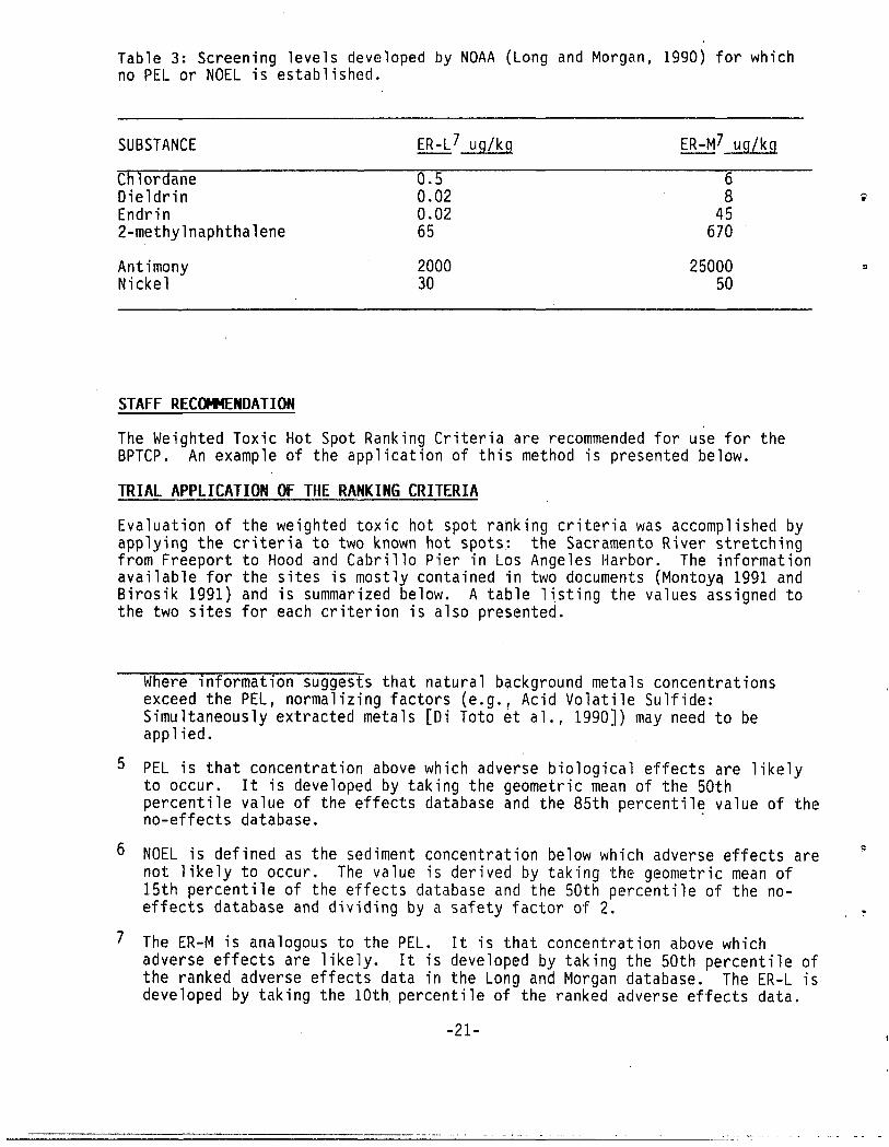
Table 3: Screening levels developed by NOAA (Long and Morgan, 1990) for whichno PEL or NOEL is established.

SUBSTANCE ER-L7 ug/kg ER-M7 ug/kg

Chlordane 0.5 6Dieldrin 0.02 8 ~

Endrin 0.02 452-methylnaphthalene 65 670

Antimony 2000 25000 ;

Nickel 30 50

STAFF RECOMMENDATION

The Weighted Toxic Hot Spot Ranking Criteria are recommended for use for theBPTCP. An example of the application of this method is presented below.

TRIAL APPLICATION OF THE RANKING CRITERIA

Evaluation of the weighted toxic hot spot ranking criteria was accomplished byapplying the criteria to two known hot spots: the Sacramento River stretchingfrom Freeport to Hood and Cabrillo Pier in Los Angeles Harbor. The informationavailable for the sites is mostly contained in two documents (Montoya 1991 andBirosik 1991) and is summarized below. A table l~sting the values assigned tothe two sites for each criterion is also presented.

Where information suggests that natural background metals concentrationsexceed the PEL, normalizing factors (e.g., Acid Volatile Sulfide:Simultaneously extracted metals [Di Toto et al., 1990]) may need to beapplied.

5 PEL is that concentration above which adverse biological effects are likelyto occur. It is developed by taking the geometric mean of the 50thpercentile value of the effects database and the 85th percentile value of theno-effects database. .

6 NOEL is defined as the sediment concentration below which adverse effects arenot likely to occur. The value is derived by taking the geometric mean of15th percentile of the effects database and the 50th percentile of the no­effects database and dividing by a safety factor of 2.

7 The ER-M is analogous to the PEL. It is that concentration above whichadverse effects are likely. It is developed by taking the 50th percentile ofthe ranked adverse effects data in the Long and Morgan database. The ER-L isdeveloped by taking the 10th. percentile of the ranked adverse effects data.

-21-

As summarized by Montoya (1991), the U.S. Geological Survey has reported waterhardness and both dissolved and total concentrations of a variety of metals atthe Sacramento River site for a number of years in both wet and dry seasons.Similar data has been produced by the Central Valley Regional Water QualityControl Board as recently as 1991, and the Regional Water Board has performedthree-species water toxicity testing in recent years. The State Water Board'sToxic Substances Monitoring Program has reported levels of organic chemicals andmetals in game and other fish collected annually at Hood since 1977. The FDAAction Levels are not exceeded but there is a human health warning for mercury(Hg) in Striped Bass. Other relevant information is the presence of anendangered species, winter run chinook salmon (Steinhart, 1990); demonstratedchronic toxicity in multiple species; exceedance of NAS DDT levels; and regularlyexceeded water quality objectives for metals.

Data for the Cabrillo Pier area of Los Angeles Harbor consists largely of arecent human health risk assessment (Pollock et al., 1991). Human health impactsare demonstrated by a sportfishing health advisory against the consumption ofresident species caught in the vicinity of Cabrillo Pier. The hazardoussubstance of concern is DDT, a carcinogen. An endangered species, 'CaliforniaLeast Tern, is present in the area, and exceedance of NAS DDT levels have beenreported.

Areal extent of both sites is relatively difficult to judge because the mediaused to qualify the sites (water in the Sacramento River and fish at CabrilloPier) show greater movement than sediment. Nevertheless, it is safe to assumethat both are larger than 50 acres. Both sites are also similar in that thepollutant sources are multiple and partially accounted for. Metals in theSacramento River can originate from urban runoff, point source discharges,agricultural practices, acid mine drainage, and other sources. DDT and PCB infish caught from Cabrillo Pier can originate from widely scattered reservoirs insediment, urban runoff, and perhaps aerial deposition. Both sites are similar inthat improvement is unlikely to occur soon without intervention.

The two sites differ, however, in their potential for implementation of anintegrated prevention strategy. Controlling metals in the river may besuccessful because the variety of sources can be controlled through wastedischarge requirements; controlling the sources of DDT and PCB is probably notpossible with waste discharge requirements. Finally, due to widespread interestin the health of the Delta and concern for threats to human health at CabrilloPier, both of these sites are likely to gain the interest of multiple agencies.

Ranking criteria scores for these two known toxic hot spots are presented inTable 4. In summary, the Sacramento River hot spot scored higher than theCabrillo Pier site. This was due in large part to the greater chemical andaquatic life impacts and a greater the likelihood of success of an integratedcontrol strategy, these higher values were somewhat compensated for by a greaterhuman health impact at Cabrillo Pier.

-22-

Table 4: Ranking Criteria Scores for Two Known Hot Spotsthe Sacramento River (Freeport to Hood) and Cabrillo Pier

Known Hot SpotSacramento River, L.A. Harbor,Freeport to Hood Cabrillo PierCriterfa

1. Human health impact

a. Potential exposure Human HealthAdvisory (Hg) 5

Human healthadvisory 5

b. Hazard Non-Carcinogen 3with RFD

Carcinogen 5with cancerpotency

c. Total score (a x b)

2. Beneficial use impacts

a. Endangered species

b. Aquat ic 1He

c. Chemical measures ~

i . Tissue residues

i i . Water objective

iii. Sediment values

Total score

3. Areal extent

4. Pollutant source

5. Remediation potential

6. Multiple agencies

15

Endangered speciespresent 5Chronic toxicity

3 x 2 = 6

DDT NAS levelexceeded 3Metals regularlyexceeded 4No data 0

7 x 2 = 14

>50 acres 8

Metals in riverwater from multi­ple sources

3 x 2 = 6Improvement un-1ike ly withoutintervention byan integratedstrategy

4 x 3 = 12Avoiding Delta im­pacts wi 11 1ike lyinterest multipleagencies 10

25

Endangered sp.present 5Not demonstrated

o

DDT NAS levelexceeded 3

No data0

No data 0

3 x 2 = 6

>50 acres 8

DDT &PCB infish from multi­ple sources

3 x 2 = 6Improvement un­likely withoutintervention butstrategy is·un­clear4 x 1 = 4

Remediating theidentified problemsinterests NOAA

10

Cumulative Score 86=

64=

-23-

•

RA~OCI~G Of POT[~TIAl HOT SPOTS

The BPTCP will conduct confirmatory work on potential hot spots to determine ifthey are known toxic hot spots. Since a large number of potential hot spotsare likely to be identified, some manner of scheduling the confirmatory work isneeded.

In contrast to known hot spot ranking, Potential Hot Spots have s~bstantially

less information available for ranking purposes. Furthermore, since monitoringcosts are much lower than probable remediation costs, the ranking of sites formonitoring purposes does not justify the level of detail used for known toxichot spot ranking. Consequently, ranking of these sites is less quantitative,consisting simply of the grouping of sites into high, medium, and lowprobability of qualifying as a known hot spot. The predominant types ofinformation available for ranking are State Mussel Watch (SMW) tissue levels,sediment contaminant levels, and, less frequently, toxicity testing. Otherkinds of data which are only occasionally available include organismimpairment, community degradation, and water contaminant levels.

The highest rank is reserved for sites that are most likely to qualify as knownhot spots due to the existence of data indicative of high risk and falling intoone of the five conditions for qualification as a known toxic hot spot. Suchdata will include positive toxicity testing results, tissue contaminant levelsapproaching NAS, FDA, or OEHHA protective levels, and occasionally otherappropriate data. Sediment contaminant data are not included because nochemical-specific sediment quality objectives have been adopted in waterquality control plans. Generally, old information will have less importancethan recent data, unless the recent data is not particularly useful in judgingthe likelihood for known hot spot qualification. For example, recent positivetoxicity tests will probably be considered equivalent to screening andtherefore require confirmatory toxicity testing. Conversely, recent SMWresults below NAS, FDA, or OEHHA protective levels will probably be judgedunworthy of further tissue testing if territorial fish are unavailable at thatsite.

The "medium" rank consists of sites with high sediment contaminant levels, asjudged first using the PEL sediment screening values, and the values from Longand Morgan (1990) for additional substances where an ER-M is available.Sampling and analysis of fish tissue will focus on SMW sites with EDLs over 85unless the results of high rank sites show that fish are unavailable orincapable of concentrating pesticides, PCB, or mercury above protective levels.

Remaining sites are of low rank and consist predominantly of sedimentcontaminant levels below ER-M, PEL values and/or SMW EDL 85.

-24-

REFERENCES

Anderson, B.S., J.W. Hunt, S.L. Turpen, A.R. Coulon, M. Martin, D.L. McKeown andF.H. Palmer. 1990. Procedures manual for conducting toxicity tests developedby the marine Bioassay Project. California State Water Resources ControlBoard 90-10WQ. Sacramento, California. 113 p.

ASTM. 1987. Standard practice for conducting static acute tests with larvae offour species of bivalve molluscs.' Procedure E724-80. Annual book"of ASTM i

standards; water and environmental technology. Vol 11.4: 382-388. AmericanSociety for Testing and Materials, Philadelphia, PA.

ASTM. 1991. Designation E,1367: Standard guide for conducting 10-day staticstatic sediment toxicity tests with marine and estuarine amphipods. Volume11.04: Pesticides; resource recovery; hazardous substances and oil spillresponses; waste disposal; biological effects. Annual book of standards;water and environmental technology. American Society for Testing andMaterials, Philadelphia, PA.

Birosik, S. 1991. Monitoring Plan for San Pedro Bay. Regional Water QualityControl Board, Los Angeles Region.

Chapman, P.M. and J.D. Morgan. 1983. Sediment bioassays with oyster larvae.Bull. Environ. Contam. Toxicol. 31: 438-444.

Cohen, D.B. 1993. Memorandum to Jesse M. Diaz regarding: Maximum Tissue ResidueLevels (MRTLs) Developed for the Inland Surface Waters Plan (ISWP) and theEnclosed Bays and Estuaries Pl~n (EBEP). January 19, 1993.

Department of Fish and Game, Marine Pollution Studies Laboratory. 1992. QualityAssurance Project and Plan for Toxicity Testing of Bay and Estuarine Water and'Sediment: Bay Protection and Toxic Clearyup Program.

DeWitt, T.H., R.C. Swartz, J.D. Lamberson. 1989. Measuring the acute toxicityof estuarine sediments. Environ. Toxicol. and Chern. 8: 1035-1048.

Diaz, J.M. 1991. Memorandum to Regional Board Executive Officers regardingupdate of the Regional Water Quality Assessments. August 2, 1991

Dinnell, P.J., J. Link, and Q. Stober. 1987. Improved methodology for sea urchinsperm cell bioassay for marine waters. Arch. Envir. Cont. and Toxicol.16: 23-32.

Di Taro, D.M., J.D. Mahony, D.J. Hansen, K.J. Scott, M.B. Hicks, S.M. Mayr, andM.S. Redmond. 1990. Toxicity of Cadmium in Sediments: The Role of AcidVolatile Sulfide. Environmental Toxicology and Chemistry, Vol. 9, pp. 1487-1502. 1990. '

-25-

EPA. 1992. Sea urchin (Strongylocentrouts purpuratus) fertilization test method.Final Draft. Gary A. Chapman, U.S. Environmental Protection Agency. ERL ­Pacific Ecosystems Branch, Newport, Oregon.

Florida Coastal Management Program, Florida Department of EnvironmentalRegulation. 1993. Development of an Approach to the Assessment of SedimentQuality in Florida Coastal Waters. Prepared by D.O. MacDonald, K. Brydges,and M.L. Haines, MacDonald Environmental Sciences Ltd., January 1993.

Horning, W.B. II and C.I. Weber (eds.). 1985. Short-term methods for estimatingthe chronic toxicity of effluents and receiving waters to freshwaterorganisms. Environmental Monitoring and Research Laboratory - CincinnatiOffice of Research and Development. U.S. Environmental Protection Agency,Cincinnati, Ohio. EPA/600/4-85/014.

Hunt, J.W., B.S. Anderson, S.L. Turpen, H.R. Barber, D.L. McKeown, F.H. Palmerand M. Martin. 1991. Marine Bioassay Project Sixth Report: Interlaboratoycomparisons and protocol development with four marine species. Report #91-21­WQ. State Water Resources Control Board, California.

Johns, D.M., T.C. Ginn and D.J. Reish. 1990. The juvenile neanthes sedimentbioassay. Puget Sound Notes, No. 24, U.S. EPA, Seattle, WA.

Long, E.R. and L. Morgan 1990. The potential for Biological Effects of Sediment­sorbed Contaminants Tested in the National Status and Trends Program. NOAATechnical Memorandum NOS OMA 52.

Middaugh, D.P., M.J. Hemmer, and E.M. Lores. 1988. Teratological effects of2,3-dinitrophenol, produced water, and naphthalene on embryos of the inlandsilverside Menidiaberyllina. Dis. Aquat. Org., 4,53 - 65.

Montoya, B.L. 1991. An Analysis of the Toxic Water Quality Impairments in theSacramento-San Joaquin Delta/Estuary. Regional Water Quality Control Board,Central Valley Region.

Mount, 0.1. and T.J. Norberg. 1984. A seven-day life-cycle cladoceran test.Environ. Toxicol. and Chern. 3: 425-434.

Nebecker, A.V., M.A. Cairns, J.H. Gakstatter, K.W. Maleug, G.S. Schuytema, andD.F. Krawezyk. 1984. Biological methods for determining toxicity ofcontaminated freshwater sediments to invertebrates. Environ. Toxicol. andChern. 3:617-630.

Peltier, W.H., and C.I. Weber. 1985. Methods for measuring the acute toxicity ofeffluents to freswater and marine organisms. Environmental Monitoring andSupport Laboratory - Cincinnati Office of Research and Development. U.S.Environmental Protection agency, Cincinnati, Ohio. EPA/600/4-85/013.

-26-

Pollock, G.A., I.J. Uhaa, A.M. Fan, J.A. Wisniewski, and I. Witherell. 1991.A study of Chemical Contamination of Marine Fish From Southern California, II.Comprehensive Study. California Environmental Protection Agency, Office ofEnvironmental Health Hazard Assessment.

Spehar, R.L., D.K. Tanner and J.H. Gibson. 1982. Effects of kelthane and pydrinon early life stages of fathead minnows (Pimephales promelas) arid amphipods(Hyalella azteca). In J.G. Peatson, R.B. Foster and W.E. Bishop, eds.,Aquatic Toxicity and Hazard Assessment: Fifth Conference. STP 766. American z

Society fior Testing and Materials, Philadelphia, PA. pp. 234-244.

State Water Resources Control Board. 1990 .• California Ocean Plan.Resolution No. 90-27.

State Water Resources Control Board. 1991. California Enclosed Bays andEstuaries Plan. Resolution No. 91-33.

State Water Resources Control Board. 1991. California Inland SurfaceWaters Plan. Resolution No. 91-33.

Tetra Tech. 1986. Recommended Protocols for measuring selected environmentalvariables in Puget Sound. Prepared for the Puget Sound Estuary Program by:Tetra Tech Inc., 11820 Northup Way Bellevue, WA 98005. March, 1986.

U.S. EPA. 1990. Hazard Ranking System; Final Rule. Federal Register, Vol. 55,No. 241, Friday, December 14, 1990, pp. 51532 -51667.

Water Quality Coordinating Committee. 1991. The Clean Water Strategy: ProposedCriteria and Method for: Phase II: Prioritizing Water Body Concerns,Phase III: Prioritizing Actions to Address Concerns.

-27-

-------------_._-----_.. _- '-'--- - .--

APPH101)( 1

'THE CLEAN" ~ ~

WATER STRATEGYi"":

GUIDANCE fOR

WATER BODY BASEDDECISION MAKING

-28-

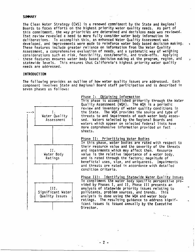
SU~Y

The Clean Water Strategy (CWS) is a renewed commitment by the State and RegionalBoards to focus efforts on the highest priority water quality needs. As part ofthis commitment, the way priorities are determined and decisions made was reviewed.That review revealed a need to more fully consider.water body information indeliberations. To accomplish this, an enhanced Water Quality Assessment was'developed, and improvements were made to reinforce water body based decision making.These features include greater reliance on information from the Water QualityAssessment, a comprehensive evaluation of needs, and a systematic way of weighingconsiderations such as risk, feasibility, cost/benefit, and trade-offs. Applyingthese features ensures water body based decis'ion making at the program, region, andstatewide levels. This ensures that California1s highest priority water qualityneeds are addressed.

INTRODUCTION

The following provides an outline of how water quality issues are addressed. Eachcomponent involves State and Regional Board staff participation and is described inseven phases as follows:

---> I.Water Quality

Assessment

II.. Water Body

Ratings

III.Significant WaterQuality Issues

.'

f

Phase I: Obtaining InformationThis phase is accomplished primarily through the WaterQuality Assessment (WQA). The WQA is a periodicreview and inventory of water quality conditions inthe State. The WQA provides the source and type ofthreats to and impairments of each water body asses­sed. Waters selected by the Regional Boards andwaters which appear on selected federal lists havemore comprehensive information provided on factsheets.

Phase II: Prioritizing Water BodiesIn this phase, water bodies are rated with respect totheir resource value and the severity of the threatsand impairments which may affect them. Resourcevalue is the relative importance of a water body,and is rated through the factors; magnitude ofbeneficial uses, size, and uniqueness. Impairmentsand threats are rated in accordance with detailedcondition criteria.

Phase III: Identif in Statewide Water ualit IssuesTo comp iment t e water body specific perspective pro­vided by Phases I, and II, Phase III presents ananalysis of statewide priority issues relating topollutants, problem sources, and trends. Thisanalysis is done using the WQA and water bodyratings. The resulting guidance to address signif­icant issues i~ issued annually by the ExecutiveDirector.

- 2 -

Phase V: AllocationThe allocation or adjustment of resources reflectingPhase IV priorities is made through budgetiri~ ,decisions.

Phase VII: ResultsResults are determined through water quality mon­itoring and management tracking of programs andcontracts. This final phase enables measurementof the progress and effectiveness of the actionstaken.

Phase VI. ImplementationResources are deployed by appropriate organizationsaccording to the allocation in Phase V.

IV.Action

Priorit ies

V.Allocat ion

VI.Implementation

VI I.Results

<--

Phase IV; Prioritizing ActionsA~t ~ors' ~9 addr¢~~ th~'~'~t~C~P~y priQrH ~e,~ ~WA ~ j~~nlflcant lssues ldentlflealn"Phases II 'anH"III 'ate:'evaluated for feasi~njiY": cQst/p~hefH,'and'H~f'<~c6ncetn~~ Priori~ies'ar~ th~nlqet¢rmired ~y ~4l~~ncing lssues suc~ .s ~r~v~ritiqrCv~. r~storation

efforts, work dealirg ~ith ~ifferent poll~tants anAproblem sources and the level pf ~fforts 1" e,~h .type of water body. . .""

The remainder of this document deals with Phases I through IV where initial CleanWater Strategy efforts have concentrated.

PHASE I: OBTAINING INFORMATION

The Water Quality Assessment (WQA) provides information on water quality conditionsand the pollutants and sources of concern. It is a single integrated data baseapplicable to all water quality program needs. ' .

The WQA includes the most important waters in the state (2500 were included in1991). Information includes size, resource value and condition ratings, descriptionof concerns (location, pollutants, and probable sources), and an accounting of thefederal lists. All information is maintained by the Regional Boards. '

The WQA data base can be used to provide various reports related to waters,pollutants and sources, etc. These reports assist program targeting on waters andthe analysis of statewide issues.

PHASE II: PRIORITIZING ~~TER 80DIES

Water quality information obtained in Phase I is translated into water pody ratirg~

in Phase II. Lists of these rated waters assist the development of program~'regional, and general statewide priorities.

- 3 -

1RAT I NG S

3 5

A few beneficialuses. Low use.

Sever~l importantbeneficial uses. Mod­erate use.

Many importantbeneficial uses.High use.

2b. Water Body Size

This is the aerial extent of 'the water body. The rating scale varies by waterbody type using the units in the Water Quality Assessment.

1 2RAT I NG S

3 4 5

Rivers andStreams (mi) > 100 70-100 40-70 15-40 0-15

Lakes, Reser­voirs, &Saline Lakes (ae). > 5000 2500-5000 1000-2500 200-1000 0-200

Ground Water(sq-mi) > 500

Bays &Harbors (ac) >10000

200-500 100-200 50-100

2500-10000 1000-2500 200-1000

Estuaries (ac)

Wetlands (ac)

> 2500

> 2500

1000-2500

1000-2500

500-1000 200-500

500-1000 200-500

0-50

0-200

0-200

0-200

2c. Uniqueness (surface waters only)

An indicator of unique or exceptional characteristics of the water body notaccounted for in other resource value factors. The criteria and range ofratings for this f~ctor are:

1RAT I NG S

2 3 5

Water body supportscritically importantor unique ecosystem.Examples includeNational EstuarineSanctuaries, Wild andScenic Rivers (onlyWild and Scenic por­tion receives..·"l"rating). .

Presence of threatenedor endangered species(RARE BU), or slightlyless important exampleof "I".

RegionallyUnconnnon

Common

- 5 -

2d. Dependence (ground water only)

An indicator of the extent to which the overlying community or the statedepends on the ground water basin. The criteria and range of ratings for thisfactor are:

1

. Overlying area entir­ely dependent onground water for mu­nicipal purposes(sole source), or

All ground wateris used and is pre­dominantly for mun­icipal uses in over­lying area, exportareas, or both.

RAT I ~ G S2

High municipal depen­dence on ground waterbasin, or total depen­dence for purposes,other than municipal.

3

Moderate tosignificantdependence onground waterbasin.

5

Ground Waternot heavilyre lied on.

3. Each water body is assigned a CONDITION rating reflecting the level of threatto or impairment of beneficial uses. Like resource value, condition is ratedon a scale from one to five. One represents highly threatened or. gros~ly

impaired.

Condition ratings are assigned for each threat to or impairment of a waterbody. These are recorded on Water Quality Assessment fact sheets. Wheremultiple concerns exist, an overall condition rating is assigned to enablestatewide comparisons.

The following criteria is used to provide consistent statewide conditionratings.

3a. Degree of Impairment. This is an indication of the magnitude of impairment ofwater quality. If unknown, indicate "UNK."

RAT I i\l G S1 3 5

Bacteria Longstanding Periodic health Objectives some-continuous de- warnings. times or slight-clared health ly violated.warnings.

BOD . Severe DO Sag Occasional DO Objectives some-causing fish Sags. times or slight-kills. . ly violated.

Metals & . Health warnings No health warn- Minor elevationTrace [le- for fish or ings, but eleva- of leve.ls inments & shellfish can- ted levels in fish and shell-Organics sumption. fish or shell- fish

fish.

- 6 -

Metals &Trace Ele­ments &Organics(contld)

1

· Drinking waterstandard ex­ceeded in ex­isting publicwater supply.

· Critical lifestages com­pletely unsup­ported.

RAT I NG S3

Drinking waterstandard ex­ceeded, exist­ing publicwater supply,not affected.

Critical lifestages onlypai't.ially sup­ported.

5

Objectives some­times or slight­ly violated.

Objectives some­times or slight­ly violated.

Overall absence Benthic organ­of benthic org- isms adverselyanisms. affected.

Sediments con­taminated, butno noticeablechange in ben­thic popula­tion.

Nitrate

Nutrients

· Drinking waterstandard ex­ceeded inexisting publicwater supply.

· Severe constantDO Sag causingfish kills, se~

vere odors, sig­nificant publiccomplaints.

Drinking waterstandard ex­ceeded, publicwater supplynot affected,individualdrinking sup~

plies affected.

Occasional DOSags, FrequentAlgal Blooms,laste and odorproblems indrinking water.

Objectives some­times or slight­ly violated.

Objectives some­times or slight­ly violated.

Resi:rictcd u~e

C'f existing Ag,supply.

Sa 1'i 11 it ~I · Restricted useof existingpub Ii c watersupply.

· Widespread fish Periodic fishkills. ki~ls &overall

population de­cline.

Objectives some­timps or slight­ly violated.

Objectives some­times or slight­ly vioiated.

Critical 'lifestages com­pletely unsup­ported.

Critical lifestages onlypartially sup­ported.

Objectives some­times or slight­ly violated.

Siltation . Widesprpad dis- Siltation oftruction of some spawningspawning areas. areas.

- 7 -

Abnormal turbid­ity.

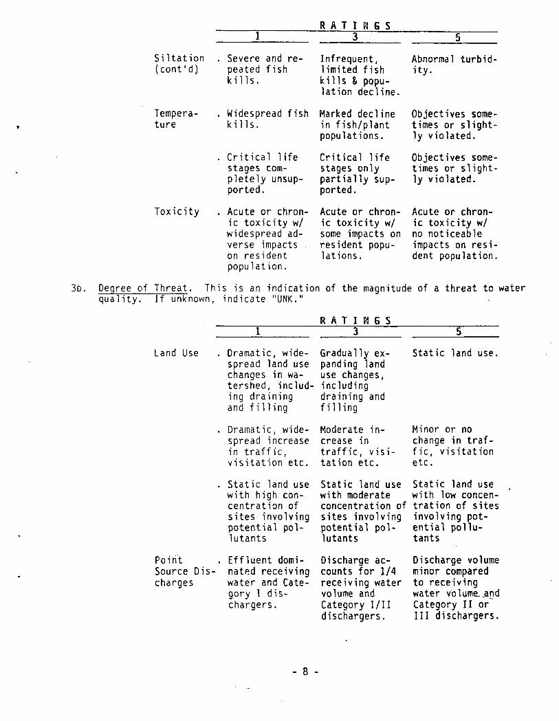
1RAT I NG S

3 5

Siltation(cont'd)

Severe and re­peated fishkills.

Infrequent,limited fishkill s & popu­1ation decline.

Abnormal turbid­ity.

Widespread fish Marked declinekills. in fish/plant

populations.

Tempera­ture

Critical lifestages com­pletely unsup­ported.

Critical lifestages onlypartially sup­ported.

Objectives some­times or slight­ly violated.

Objectives some­times or slight­ly violated.

Acute or chron­ic toxicity w/no noticeableimpacts on resi­dent population.

Acute or chron­ic toxicity w/some impacts onresident popu­lations.

Toxicity . Acute or chron-ic toxicity w/widespread ad­verse impactson residentpopulation.

3b. Degree of Threat. This is an indication of the magnitude of a threat to waterquality. If unknown, indicate "UNK."

1RAT I N G S

3 5

Land Use Dramatic, wide­spread land usechanges in wa­tershed, includ­ing drainingand filling

Graduallyex­panding landuse changes,includingdraining andfilling

Static land use.

Dramatic, wide­spread increasein traffic,visitation etc.

Moderate in­crease intraffic, visi­tation etc.

Minor or nochange in traf­fic, visitationetc.

Static land usewith high con­centration ofsites involvingpotential pol­lutants

Static land use Static land usewith moderate with low concen­concentration of tration of sitessites involving involving pot­potential pol- ential pollu-lutants tants

Point . Effluent domi-Source Dis- natp.d receivingcharges water and Cate-

gory I dis­chargers.

Discharge ac­counts for 1/4receiving watervolume andCategory I/IIdischargers.

Discharge volumeminor comparedto receivingwater volume.._andCategory II or­III dischargers.

- 8 -

1RAT I NG S

3 5

Trends . Dramatic con- Moderate con-stituent level stituent lev-increase in el increaseshort time per- over time.iod.

Minor or no con­stituent levelincrease overtime.

4. Upon completion of the resource value 'and condition ratings, the rated waterbodies are listed in descending order of resource value for each water bodytype. This emph~sizes resource value as the first priority consideration.Waters with the same resource value are arranged in descending order ofcondition ratings to provide further rankings as follows:

WATER BODY TYPE

Waters wlthResource Value of: Impaired List Threatened List

1 Waters in descending severity of impairmentor threat with a resource value of 1.

2 as above for RV=2

3 as above for RV=3

4 as above for RV=4

5 as above for RV=5

IPHASE III: STATEWIDE WATER QUALITY ISSUES

Phase III involves an analysis of the WQA and the water body rankings. Thisanalysis is used to assist the annual preparation of guidance to staff onsignificant watef quality issues. This guidance, in conjunction with Phase II water~body priorities, is used to solicit action proposals, direct program activities, and'to screen and evaluate actions proposed.

- 9 -

Significant issues .gu·idance includes:

a. Identification of the ,most sign'ificant :po'lilutantsand sources ,df :po"ll1:u!Vicfnaffecting California's waters.

b. Identification o,fissues requiring short ,a'nd long term'st·rategies.

c. Identificat~on ~f general actions to ~ddress the significant issues.

Issues are identified .by the Division of Water Quality Monitori"ng and Asse'sSinen'tUnit. Every January the Executive .Director issues Quidance to address issues.

Phase III products ~re not limited to the annual significant issues guidance. On anongoing basis, the Monitoring and Assessment Unit prepares distillations andsummaries of Water Quality Assessment information. These provide an additionallevel of detail and perspective to compliment the Executive Director's gtlidance.Staff should access this information as appropriate.

PHASE IV: PRIORITIZING ACTIONS

Phase IV is preceded by the solicitation of actions which reflect the prioritiesdetermined through Phases II and III. Thh assists the focusing of actions on themost significant concerns.

In Phase IV, the proposed actions addressing the needs of water bodies andpollutant/source concerns are evaluated and prioritized within available resources.Priorities are arrived at through combining Phase II and III rankings and guidancewith feasibility, cost/benefit, and risk considerations. Funding lines are drawnbased on balancing issues such as prevention vs. restoration efforts, work dealingwith different pollutants and problem sources and the level of efforts in each typeof water body (Figure 1).

The following sequence of actions occurs during Phase IV (see Figure One):

1. Phase II and Phase III priorities are distributed.

2. Actions are initially ranked in accordance with the resource value andcondition ratings of the Wcttei' body(s) with which they deal. The result is alisting formatted the same way as described in Phase II. However, these listsinclude only the water bodies for which actions are proposed. For example,assume a program needs to rank actions pertaining to five rivers; a, b, c, d,e. The following list results:

- 10 -

Phase IV

Phase III Interim Priorities

Water body ratings and significantissues priorities

I

Feasibility Considerations

- Technical- Economic/Financial- Institutional- Political/Legal/Environmental/Social

I

Strategic Considerations

Various factors may cause feasible proposals to move up or down onpriority lists. These factors include:

- Cost/Benefit Considerations- Risk Evaluation- Spin-off Benefits

I

Final Balancing

Funding decisions are made palancing the dis­tribution of resources by:

- Water Body Type- Prevention, Assessment, and Cleanup Activities- Pollutant Constituent- Problem Source

I

Priority Actions

A final list of actions is determinedconsistent with available resources

- 11 -

F;gure 1

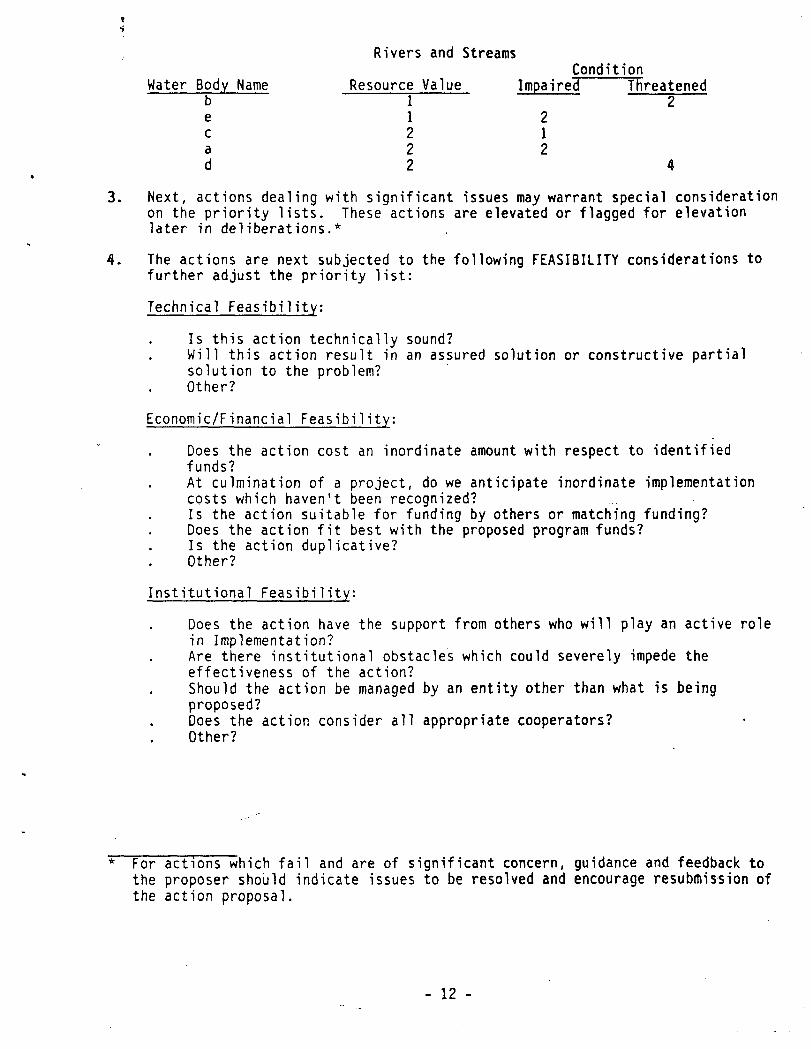
ConditionImpaired Threatened

2Water Body Name

becad

Rivers and Streams

Resource Value11222

212

4

3. Next, actions dealing with significant issues may warrant special considerationon the priority lists. These actions are elevated or flagged for elevationlater in deliberations.*

4. The actions are next subjected to the following FEASIBILITY considerations tofurther adjust the priority list:

Technical Feasibility:

Is this action technically sound?Will this action result in an assured solution or constructive partialsolution to the problem?Other?

Economic/Financial Feasibility:

Does the action cost an inordinate amount with respect to identifiedfunds?At culmination of a project, do we anticipate inordinate implementationcosts which haven't been recognized?.Is the action suitable for funding by others or matching funding?Does the action fit best with the proposed program funds?Is the action duplicative?Other?

Institutional Feasibility:

Does the action have the support from others who will play an active rolein Implementation?Are there institutional obstacles which could severely impede theeffectiveness of the action?Should the action be managed by an entity other than what is beingproposed?Does the action consider all appropriate cooperators?Other?

* For actions which fail and are of significant concern, guidance and feedback tothe proposer sho~ld indicate issues to be resolved and encourage resubmitsion ofthe action proposal.

- 12 -

Political, Environmental, Social, Legal Feasibility:

Are there severe political, environmental, social, or legal difficultieswith respect to the action?Are there legislative aspects which have not been recognized and whichcould limit the success of the action?Other?

Should an action be judged infeasible, that action will be crossed off thepriority list(s) and the reasons documented.* In instances where the staff isconcerned about one feasibility component but is not in a good position to makean ultimate judgement (such as political feasibility) that concern will bedocumented and referred for higher level review.

5. Strategic co~cerns are evaluated and may elevate or lower actions on the·priority lists. The following are considered:

Cost/Benefit: Will a low cost action yield relatively high benefits withrespect to other actions? For example, it may be advantageous to fundseveral low ranked actions rather than one more expensive high rakedaction. In order to achieve the most benefits with available funds,actions which leverage benefits may be elevated on priority lists Tor eachtype of water body.

Risk: Is the action being considered something that has to be doneimmediately, or can it wait? As a result of inaction now, will inordinatecosts or harm occur later?

Spin-off Benefits: Sometimes an action ~n one program or region can yieldinformation useful throughout the organization, or be on the critical pathfor several other actions statewide, or it may leverage significantparticipation by other parties. Actions resulting in such spin-offbenefits should be considered for elevation on priority lists.

Additional Considerations: Any concern or programatic need not coveredabove.

6. The final step in determining priorities involves balancing the distribution ofresources by:

Water Body TypePrevention; Assessment, and Cleanup ActivitiesProblem SourcePollutant Constituent

* For actions whjch faii and ar~ of ~ignificant concern, guidance and feedback tothe proposer should indicate issues to be resolved and encourage resubmission ofthe action proposal.

- 13 -

This ensures that level of efforts are balanced with respect to reducing risksin each type of water body, for each type of pollutant or problem source, andin protection/restoration activities.

Staff recommendations based on the above considerations are then forwarded tomanagement.

NOTE: This phase involves a high degree of best professional judgement. Whilethe above outlines an iterative process involving several considerations, themost important aspect is the assurance that important considerations have beenmade. In practice many of the iterations described above will occursimultaneously.

- 14 -

Examples of Water BodyBased Decision Making

Example One: Statewide Cutbacks

It is 1993 and we have beeh successful in adding 100 pqsitionsfor criticalwork this year. However, a call comes from the Department of Finance--weface ~another general five percent cut. How do we take the cut? Implementation ofthe Clean Water Strategy (CWS) will assist in making this decision.

While the CWS emphasizes water body based decision making, the ultimate goalis efficiency in reducing risk. That is, ensuring that program actions onhigher overall risk situations are covered and that the lower overall risksituations are recognized and addressed subject to available funds. The CWSwater body ratings provide important comparative relationships between watersin the State. By understanding the relationships between water bodies, it ispossible to compare actions to reduce risk, determine priorities, and adjustresources accordingly. The following represents a possible outcome of the1993 situation:

As programs have increasingly focused on higher priority risk reductionsituations, a compaction of work efforts has occurred. For program THIN,instead of barely addressing 100 situations, efforts have been concentrated on40 situations and the same funds are being used to accomplish more overal)risk reduction in the State. In this scenario the number 41 situation isunfunded. Program FAT has also seen compaction and its unfunded situationscan now be compared with number 41 in program THIN. If the highest priorityunfunded situations in each program represent the same risk, then five percent.reductions would be equal in both program~. If program FAT is addressinglower risk priorities, then this program would be targeted for reduction.Conversely, program THIN may be targeted for budget increases or redirectionaugmentations from programs such as FAT.

Example Two: Allocation of New Resources

The Abandoned Mine Program Manager has be~n directed to make recommendationsregarding $3 million in new program resources. The manager must requestproposa 1s from the Reg iana 1 Boards and draH stiiff recoInmendat ions on how the.funds should be u$ed. How ca~1 water body rankings and significant issuesguidance be used to help make recommendations on resource allocation?

First, the program manager should request th~t proposers give firstconsideration to actions addressing high resource value water bodies with themost severe threats or impairments. If the significant issues guidanceindicates any abandoned mines priorities, then these should also behighlighted in the solicitation.

Once proposals. are received, the program manager preliminarily ranks proposalsbased on water body rank~ngs. For example, if proposals were receivedrelating to the Eel River and the Sacramento River, both resource value "1"water bodies, the Sacramento River project would initially be ranked higherdue to the riverls higher level of impairment (a "1 11 impaired rating ~et!us a"3" threat). Next, guidance on significant water quality issues isconsidered. For instance. if the guidance indicatp.s that mercury problems aremost importnnt, then proposals addressing mercury should be considered for

..

...

elevation on priority lists. Similarly, if guidance is focused on abandonedmine problems affecting ground water, then this information should be kept inmind when balancing decisions between different water body types areeventually made.

Next the actions proposed are screened for feasibility. This includesinstitutional, political, legal, economic, environmental, technical, andsocial aspects. If a proposed project is feasible, then the benefits of theproposals are weighed through cost/benefit, timing, and risk considerations.For example, if the proposed Eel River project was to yield the same benefitsas the proposed Sacramento River project for significantly lower cost, the EelRiver project might be elevated above the Sacramento River project.

Finally, balancing decisions are made to distribute the $3 million.Distribution by water hody type, problem source, pollutant constituent, andprevention versus remediation efforts are all considered. Recommendations areforwarded for management review and approval.

Example Three: Managing.Current Resources

Region Ten's Stormwater Program is preparing its annual workp1an. Stablefunding is expected but it's inadequate to address all program needs. How canthe CWS improvements assist the program manager prioritize the workload.

By examining the Water Quality Assessment (WQA) the program manager canidentify waters with threats and impairments related to stormwater. Reportscan be accessed through the WQA which provide specific program targeting lists(see the Monitoring alld Assessment Unit). If more detail is needed, waterbody fact sheets might be of assistance.

The manager would then consider the ratings of the waters (included in the WQAdata base) identified above. These ratings provide the manager with waterbody relationships. In turn, the manager ensures protection of the highestresource value waters through safeguards such as the permitting of stormwaterdischarges, inspections and enforcement. Similarly, for waters impaired bystormwater, the manager ensures that consideration for priority actions firstaddress the highest valued, most severely impaired waters. After all costsand needs are considered, the manager aligns fiscal resources with water bodypriorities. Again, the Executive Director's significant issues guidanceshould also be consulted for related concerns.

APPENDIX 2

HAZARD RANKING SYSTEM

The Hazard Ranking System (HRS) was developed as part of the implementation ofthe national superfund program. The HRS is designed to score the relativethreat associated with actual or potential releases of hazardous substancesfrom specific sites and to assign the site to the National Priority List forSuperfund cleanup. The HRS provides a numerical value derived from theassessment of four different environmental pathways each evaluated for threespecific factors. The pathways are (1) ground water migration, (2) surfacewater migration, (3) soil exposure, and (4) air migration. The three factorsare (1) the likelihood of release, (2) waste characteristics, and (3) targets.A summary of the HRSis provided below beginning with steps common to the fourpathways, followed by a brief description of an evaluation of the surface waterpathway.

The first step in developing a pathway score is to identify sources ofhazardous substances. In the context of the HRS, sources mean Il any area wherea hazardous substance has been deposited, stored, disposed, or placed, plusthose soils that have become contaminated from migration of a hazardoussubstance II (Federal Register, Vol. 55, No. 241, December 14, 1990). Thespecific substance(s) of concern are then identified by either documentation(labels, manifests, monitoring report, etc.) or observation.

At this point the factor assessment begins with the evaluation of thelikelihood of release. When an observed release is demonstrated, a maximumvalue (550) is assigned for this factor. An observed release is definedexplicitly but generally can be considered to be samples with substances atconcentrations three times the background concentration or, if no backgroundvalue exists, concentrations above the quantitative limit. If an observedrelease is not identified then the potential for release is evaluated on apathway specific basis (summarized below for the surface water pat~way).

The next step is evaluation of waste characteristics factor. This involvesevaluating and scoring toxicity and quantity, and then multiplying the scoresfor these characteristics together. The final waste characteristics value fora pathway is derived from a table provided in the regulations.' Wastecharacteristics are evaluated for the substance with the greatest hazard forthe pathway.

To determine which substance poses the greatest hazard, a toxicity factor valueis combined with the mobility, persistence, bioaccumulation factor. Thetoxicity factor is derived from one of three information sources: (1) forcarcinogens the cancer potency factor combined with the substanceclassification as known or potential carcinogen is used, (2) for noncarcinogens •a reference dose (RfD) is used where available, or (3) for noncarcinogens where

-44-

•

an RfD is not available, an acute toxicity value is used. The value of thetoxicity factor is dependent on the numerical value of each of thesecharacteristics (carcinogenicity, reference dose, acute toxicity) and isderived from a table provided in the regulations. Several clarifyingconditions apply to this evaluation.

Once a toxicity factor is identified it is multiplied by a mobility,persistence, and/or bioaccumulation factor. The choice and characterization ofthis second factor is pathway specific. Each toxicity, factor is multiplied byits respective mobility, persistence, bioaccumulation factor, and the substanceyielding the highest product is selected as the hazardous substance of concernfor waste characterization. .

The second major factor to evaluate for waste characterization is wastequantity. This factor is evaluated using a hierarchy of four measures:(1) hazardous constituent quantity, (2) hazardous waste stream quantity,(3) volume, and (4) area. The first of the measures (in order presented) forwhich there is adequate information is used to develop the quantity factor.With some exceptions, the hazardous wastes identified for CERCLA (ComprehensiveEnvironmental Response, Compensation, and Liability Act) purposes constitutethe substances of concern for quantity assessments. The quantity associatedwith each source is characterized (assigned a value according to tablesprOVided) and the sum of the scores for all sources is used to select a finalquantity factor for the pathway. Several specific conditions are consideredwhen determining whether adequate information is available to invoke one of thehiearchical measures.

The final value for the waste characteristics factor is obtained by multiplyingthe toxicity factor, adjusted according to the mobility, persistence, and/orbioaccumulation factor, by the quantity factor. The product of thismultiplication is then applied to a table to select the final wastecharacteristics factor. Special adjustments are made when consideringbioaccumulative substances.

The final factor score needed for developing a site score is a target score.The evaluation of targets is divided into four classes: (1) individual,(2) human population, (3) resources, and (4) sensitive environments. Eachclass is evaluated on the basis of actual or potential releases and theintensity of the exposure. The intensity of the exposure is divided intoLevel I or Level II exposures. Generally, Level I exposures are where theconcentrations of hazardous substances in specific media (i.e., water, tissue,sediment) meet or exceed available regulatory limits (benchmarks) such as waterquality standards or public health warnings or an established dietary risk.Level II exposures are again assigned to observed releases, but in this case,the appropriate benchmark value for the media-specific concentration has notbeen exceeded, or a benchmark does not exist. The final target score isdeveloped differently for each pathway and will be illustrated below forsurface water.

-45-

The development of a value for the surface water migration pathway issummarized below to illustrate the complexity and comprehensiveness of theassessment. Each of the four pathways are treated similarly, although not allpathways contain as many subdivisions as the surface migration path.

Two basic components are included in the surface migration path:(1) Overland/flood migration, and (2) Ground water to surface water migration.The Overland/flood path will be summarized for this illustration. A source ora site of contaminated sediments is identified and a target distance is defined(generally as 15 miles down gradient from the site of contamination). Theevaluation is then broken down into three parts, threat to drinking water,threat to the human food chain, and threat to sensitive environments. Each ofthese components is further subdivided to evaluate the likelihood of release,waste characteristic, and targets. The treatment of these evaluations issubstantially the same but the specific information applied within theindividual evaluations differs. The threat to drinking water evaluation willbe described as an illustration.

The likelihood of release evaluation for the drinking water threat is dividedinto observed releases and potential releases. If an observed release can beestablished, the maximum score is applied to this factor, otherwise a potentialrelease is evaluated. Observed release is explicitly defined for thisevaluation. A potential release is evaluated based on three components:(1) containment, (2) runoff, (3) distance to surface waters. For BPTeppurposes, known toxic hot spots would fall under the observed release category.

Waste characteristics for the threat to drinking water are evaluated next.This evaluation is based on two factors: toxicity/persistence and quantity.An evaluation is conducted for each substance capable of migrating from thesource to surface water. The toxicity factor is developed as described above.Persistence is based on environmental half-life (the result of the combinationof decay processes, biodegradation, hydrolysis, photolysis, and volatilization)and sediment sorption (based on log Kow )' The value for the half-life of thesubstance of concern is generated from an equation provided in the ,regulations.The persistence factor is then selected from a table, using the appropriatevalues for half-life and certain conditional characteristics of the water bodyand drinking water sources present. Toxicity and persistence are combined intoa single value using another table provided. The toxicity/persistence value ismultiplied by a quantity value (see above) and this product is applied toanother table to select the drinking water threat - waste characteristicsvalue.

The drinking water targets value is derived next. This value is based on threefactors: nearest intake, population, and resources. For the intake target andpopulation target a determination is made of whether the target is subject toobserved or potential releases of hazardous substances and whetherconcentrations meet Level I (exceed specified benchmarks) or Level II (belowspecified benchmarks) criteria. A score for the nearest intake is thendeveloped. The drinking water intake nearest to the source and within the

-46-

migr~tion path defined is identified. If thi~ intqk~ is subject to me~~yr~~

concentrations of the substances of concern (Level I or It) it i~ q~~ign~~'~score. Otherwise a score is assigned bq~ed on a dil~tion weight s~lect~q frqma table provided in the regulations.

The population servi~ed by each intake within the migration path is identified(adjusted for blenqed drinking water). The population size subject to Level I,Level II, and potential contamination is determined for the total migrationpath (summing individual intakes) and the sum of these three categories is usedas the population target value. A resource value is assigned based on the useof water for irrigation, livestock watering, water recreation area, actual ordesignated drinking water source, or for commercial food preparatiqn.

The drinking water threats-targets factor is developed by summing the valuesfor intake, population, and resources. The final drinking water threat factorscore is derived by multiplying the likelihood of release value, wastecharacteristics value, and targets values and dividing by 82,500. Theresulting value is then used to select the drinking water threat score from atable provided. This score is then combined with scores for Threat to HumanFood Chain and Environmental Threat to arrive at the score for final score foroverland/flood migration component. This score is in turn combined with ascore for ground water to surface water migration to arrive at the finalSurface Water Migration Path score. The Surface Water Migration Path score iscombined with the other three path scores using an equation provided togenerate the final site score.

-47-

APPENDIX 3

CHEMICAL SPECIFIC VALUES FOR CARCINOGENS USED FOR RANKING TOXIC HOT SPOTS. i

SUBSTANCE PEL! MTRL2 MTRL2 !!.QQ3 wgo3(dry) (Fresh)(Estu~rine) (Fresh) (Marine)mg/kg ug/kg ug/kg ug/l ug/l

~.

acrylonitrile 0.96 11aldrin 0.05 0..33 0.13 0.14arsenic 64 200 5.0 9.3benzene 1.8 110 0.34 21

benzidine 0.005 0.02beryll ium 0.15 2.5bis(2-chloroethyl)ether 0.09 4.3bis(2-ethylhexyl)phthalate 380 1300

carbon tetrachloride 4.1 72chlordane 1.1 1.2 0.00008 0.00008chloroform NA 1800 100 480

4,4 1 DDE 0.13 32.0 32.0DDT, total 0.27 32.0 32.0 0.00059 0.00061,4-dichlorobenzene 550 3600 9.9 64.0

3,3'-dichlorobenzidine 4.5 9.01,2-dichloroethane 0.6 150.01,1-dichloroethylene 0.32 18.0

dichloromethane 4.2 1400 4.6 1600.01,3-dichloropropene 0.4 60dieldrin 0.65 0.7 0.00014 0.000142,4-dinitrotoluene 0.42 35.0

1,2-diphenylhydrazine 1.0 14halomethanes NA 1800 100.0 480.0heptachlor 1.8 1.9 0.00016 0.00017heptachlor epoxide 0.8 0.8 0.00007 0.00007

~.

-48-

APPENDIX 3 (continued)CHEMICAL SPECIFIC VALUES FOR CARCINOGENS USED FOR RANKING TOXIC HOT SPOTS.

SUBSTANCE PEL MTRL MTRL !Kill !Kill~ "[dry} (Fresh}(Estuarine) (Fresh) (Estuarine)

mg/kg ug/kg ug/kg ug/1 ug/1

hexachloroethane 170 760hexachlorobenzene 6 6 0.00066 0.00069hexachlorobutadiene 1.2 140hexachlorocyclohexane (gamma) 2.5 8.1 0.019 0.062

hexachlorocyclohexane (alpha) 0.5 1.71 0.0039 0.013hexachlorocyclohexane (beta) 1.8 6 0.014 0.046isophorone 38 27N-nitrosodimethylamine 0.00006 0.7

N-nitrosodiphenylamine 370 1200pentachlorphenol 3.1 90.0 0.28 8.2PAWs (total) 28.00 0.08 0.93 0.0028 0.031acenaphthene 0.45

anthracene 0.74fluorene 0.46naphthalene 1.10phenanthrene 1.20

LMW-PAH, total 2.40benz(a}anthracene 1. 30benzo(a}pyrene 1. 70chrysene 1. 70

dibenzo(a,h}anthracene 0.32fluoranthene 3.20pyrene 1. 90HMW-PAH, total 8.50

PCB IS (tota l) 0.26 2.2 2.2 0.00007 0.000072,3,7,8-tetrachlorodibenzo-

p-dioxin 0.00007 0.00007TCDD equivalents 0.000000013 0.000000014

toxaphene 8.8 9 0.00067 0.000691,1,2-trichloroethane 2.7 1901,1,2,2-tetrachloroethane 0.86 54.0trichloroethylene 33 980

-49-

APPENDIX 3 (continued)CHEMICAL SPECIFIC VALUES FOR NONCARCINOGENS USED FOR RANKING TOXIC HOT SPOTS. "",SUBSTANCE PEL MTRL MTRL ~ WQO

((Try) (Fresh)(Estuarine) (Fresh) (Estuarine)mg/kg mg/kg mg/kg ug/l ug/l

~i

tetrachloroethylene 19 2102,4,6-trichlorophenol 50 150vinyl chloride 0.15 40acrolein 69 170antimony 0.014 4.3cadmium 7.5 0.64 NA 10** 9.3chlorobenzene NA 46'

4-chloro-3-methylphenol NA NA 3000.0bis(2-chloroisopropyl)ether 3.4 430.0chromium (VI) 240* NA NA 50.0**Chromi urn (II I) 530 11000

copper 170 NA NA ** 2.9cyanides 0.7 220.0di-n-butylphthalate 240 11001,2-dichlorobenzene 150 970 2700.0 18000.0

1,3-dichlorobenzene 22 . 150 400.0 2600.02,4-dichlorophenol NA 32 0.3diethylphthalate 1700 86002,4-dimethylphenol NA 220

dimethylphthalate 11000 1100004,6-dinitro-2-methylphenol 0.07 4.22,4-dinitrophenol 0.11 22endosu lfan-tota 1 0.25 0.5 0.056 0.0087

endrin, total 3.0 3.2 0.0023 0.0023ethyl benzene NA 1100fluoranthene 49 62 42.0 42.0

If

-50-

ApPENDIX 3 (co~ti~~~q)CHEMICAL SPECIFIC VALuES FOR NONCARCINOGENS USED FOR RANKING TOXIC HOT SPOTS.. ,.,.: 1 J'!' -."", . - . I" ' .• "'i" .,'" I' ' ..... " •• ,'.

SUBSTANCE PEL MTRL MTRL wgo WQOWy) (Fresh) (Estuarine) (fresh,) (Estl,J,arine)~g/kg mg/kg mg/kg ug/l ug/l

~~xachlorocyclopentadiene

leadmercurynicke1nitrobenzenephenolseleniumsilver

1601.4

2.5

NANA1.0280.05NANANA

75NA1.02205.46500NANA

50**0.012600**

3005.050.0**

5.00.0258.3

71.02.3

tha 11 i urntoluenetributyltinl,l,l-trichloroethanezinc 300

0.20110

1.1NA

0.732000.362NA

10000.0 30000.020.0 0.005

5000.Q* 86.0

* The PEL is based on total chromium rather than Cr(VI).

** indicates an aquatic life objective exists that may be a lower value thanlisted, due to its dependance on water hardness and/or acidity. The lowervalue of the listed or calculated value should be used.

1 PEL is that concentration above which adverse biological effects are likelyto occur. It is developed by taking the geometric mean of the.50thpercentile value of the effects database and the 85th percentile value ofthe no-effects database.

2 MTRL-Maximum Tissue Residue Level. The MTRL is calc~lated by ~ultiply~~g

the human health water quality objective in the appropriate Statewiqe Planby the che~icalls bioconcentration factor (BCF) (Cohen, 1993). MRTLs' ,,'proposed for use in the ranking system are based on the standards containe~

in the most recent version of the California Enclosed Bays ard EstuariesPl,an.

3 WQO--Water Quality Objectives are the stanqards cortained in statewiqewater quality control plans for freshwaters or enclosed bays and estuaries.These columns qo not contain the water quality objectives adopted by theState Water Board in November 1992 because these WQO have not been approvedby the Office of Administrative Law. The water quality objectives in themost recent version of the Statewide Plans should be used.

, \ . ' ,',. i

-51-

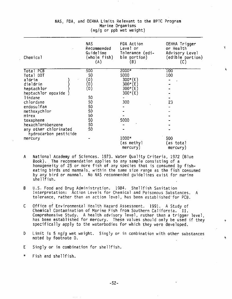
NAS, FDA, and OEHHA Limits Relevant to the BPTC ProgramMarine Organisms

(ng/g or ppb wet weight)

Chemical

Total PCBTotal DDTaldrin )dieldrin )heptachlor )heptachlor epoxide )lindanechlordaneendosu 1fanmethoxychlormirextoxaphenehexachlorobenzeneany other chlorinated

hydrocarbon pesticidemercury

NASRecommendedGuideline(whole fish)

(A)

50050

(D)(D)(D)

50505050505050'50

FDA ActionLevel orTolerance (edi­ble portion)

(B)

2000*5000300*(E)300*(E)300*(E)300*(E)

300

5000

1000*(as me. thylmercury)

OEHHA Triggeror HealthAdvisory Level(edible portion)

(C)

100100

23

500(as totalmercury)

A National Academy of Sciences. 1973. Water Quality Criteria, 1972 (BlueBook). The recommendation applies to any sample consisting of ahomogerieity of 25 or ~ore fish of any species that is consumed by fish­eating birds and mammals, within the same size range as the fish consumedby any bird or mammal. No NAS recommended guidelines exist for marineshellfish.

B u.s. Food and Drug Administration. 1984. Shellfish SanitationInterpretation: Action Levels for Chemical and Poisonous Substances. Atolerance, rather than an action level, has been established-for PCB.

C Office of Environmental Health Hazard Assessment. 1991. A Study ofChemical Contamination of Marine Fish from Southern California. II.Comprehensive Study. A health advisory level, rather than a trigger level,has been established for mercury. These values should only be used if they ~

specifically apply to the waterbodies for which they were developed.

D Limit is 5 ng/g wet weight. Singly or in combination with other substancesnoted by footnote D.

E Singly or in combination for shellfish.

* Fish and shellfish.

-52-

• A P P E ~ 0 I X F

Senate Bill 1084 (Calderon)(Statutes 1993, Chapter 1157)

Bay Protection and Toxic Cleanup ProgramAmendments and Additions to the Water Code

Chapter 5.6 of the Water Code

Amendments toSections 13392.5, 13393, 13393.5, 13394, and 13396.5

AddedSections 13394.6 and 13396.7

•

Senate Bill No. 1084

CHAPTER 1157

An act to amend Sections 13392.5, 13393, 13393.5, 13394, and 13396.5of, and to add Sections 13394.6 and 13396.7 to, the Water Code, relat­ing to water.

[Approved by Governor October 10, 1993. Filed withSecretary of State October 11, 1993.]

LEGISLATIVE COUNSEL'S DIGFSf

SB 1084, Calderon. Bays and estuaries.(1) Existing law, which is to he repealed on January 1, 1994,

requires the State Water Resources Control Board to impose annualfees applicable to all point and nonpoint dischargers who dischargeinto enclosed bays, estuaries, or any adjacent waters in thecontiguous zone or the ocean, as defined. Existing law requires thestate board, on or before January 1, 1993, to make a prescribed reportto the Legislature.

This bill would extend that repeal date to January 1, 1998. The billwould prohibit the state board from imposing a fee on anyagricultural nonpoint source discharger. The bill would extend thedue date applicable to the report to January 1, 1996.

(2) Existing law requires each California regional water qualitycontrol board that has regulatory authority for any enclosed bay orestuary to develop, by January 1, 1992, for each such bay or estuary,a consolidated data base that identifies and describes all suspectedtoxic hot spots.

This bill would instead require those regional boards to develop,by January 30, 1994, a consolidated data base that identifies anddescribes all potential hot spots.

(3) Existing law requires the state board to adopt, by July 1, 1992,general criteria for the assessment and priority ranking of toxic hotspots.

This bill would extend that date to January 30, 1994.(4) Existing law requires each regional board to complete and

submit to the state board, by July 1, 1993, a toxic hot spots cleanupplan. Existing law requires the state board to submit to theLegislature, by January 1, 1994, a consolidated statewide toxic hotspots cleanup plan.

This bill would extend the due date applicable to the toxic hot spotscleanup plan to January 1, 1998, and the due date applicable to theconsolidated statewide toxic hot spots cleanup plan to June 30, 1999.

. (5) Existing law requires the state board to adopt sedimentquality objectives for toxic pollutants.

This bill would require the state board to consider prescribedfederal sediment criteria for toxic pollutants, and to take specified

92 90

Ch. 1157 -2-

•

action, in connection with the adoption of sediment qualityobjectives.

The bill would require the state board to establish a prescribedadvisory committee to assist the state board in carrying out specifiedwater quality functions relating to bays and estuaries.

(6) The bill would require the state board, in consultation with theState Deparbnent of Health Services, to contract with anindependent contractor to conduct a study to detennine the adversehealth effects of urban runoff on swimmers at urban beaches, asprescribed. The bill would make legislative findings and declarations.

The people of the State of California do enact as follows:

SECfION 1. The Legislature finds and declares all of thefollowing:

(a) A significant source of beach contamination results fromurban runoff.

(b) The public use of beaches has declined 25 to 30 percent. Thatdecline is attributable in part to concerns about contamination.

(c) The number of beach closures by local public officialscontinues to increase each year.

SEC. 2. Section 13392.5 of the Water Code is amended to read:13392.5. (a) Each regional board that has regulatory authority

for one or more enclosed bays or estuaries shall, on or before]anuary30, 1994, develop for each enclosed bay or estuary, a consolidateddata base which identifies and describes all known and potentialtoxic hot spots. Each regional board shall, in consultation with thestate board, also develop an ongoing monitoring and surveillanceprogram that includes, but is not limited to, the followingcomponents:

(1) Establishment of a monitoring and surveillance task force thatincludes representation from agencies, including, but not limited to,the State Deparbnent of Health Services and the Deparbnent of Fishand Game, that routinely monitor water quality, sediment, andaquatic life.

(2) Suggested guidelines to promote standardized analyticalmethodologies and consistency in data reporting.

(3) Identification of additional monitoring- and analyses that areneeded to develop a complete toxic hot spot assessment for eachenclosed bay and estuary.

(b) Each regional board shall make available to state and localagencies and the public all information contained in the consolidateddata base, as well as the results of new monitoring and surveillancedata.. SEC. 3. Section 13393 of the Water Code is amended to read:

13393. (a) The state board shall adopt sediment qualityobjectives pursuant to the workplan submitted pursuant.to Section13392.6.

92 140

-3- Ch. U~

(b) The state board shall adopt the sediment quality objectivespursuant to the procedures established by this division for adoptingor ,amending water quality control plans. The sediment qualityobjectives shall be based on scientific information, including, but notlimited to, chemical monitoring, bioassays, or established modelingprocedures, and shall provide adequate protection for the mostsensitive aquatic organisms. The state board shall base the sedimentquality objectives on a health risk assessment if there is a potentialfor exposure of humans to pollutants through the food chain to ediblefish, shellfish, or wildlife.

(c) (1) Notwithstanding subdivision (a), in adopting sedimentquality objectives pursu~nt to this section, the state board shallconsider the federal sediment criteria for toxic pollutants that arebeing prepared, or that have been adopted, by the EnvironmentalProtection Agency pursuant to Section 1314 of Title 33 of the UnitedStates Code.

(2) If federal sediment criteria have been adopted, the state boardshall review the federal sediment criteria and determine if thecriteria meet the requirements of this section. If the state boarddetermines that a federal sediment criterion meets the requirementsof this section, the state board shall adopt the criterion as a sedimentquality objective pursuant to this section. If the state boarddetermines that a federal sediment criterion fails to meet therequirements of this section, the state l;loard shall adopt a sedimentquality objective that meets the requirements of this section.

SEC. 4. Section 13393.5 of the Water Code is amended to read:13393.5. On or before January 30, 1994, the state board, in

consultation with the State Department of Health Services and theDepartment of Fish and Game, shall adopt general criteria for theassessment and priority ranking of toxic hot spots. The criteria shalltake into account the pertinent factors relating to public health andenvironmental quality, including, but not limited to, potentialhazards to public health, toxic hazards to fish, shellfish, and wildlife,and the extent to which the deferral of a remedial action will result,or is likely to result, in a significant increase in environmentaldamage, health risks, or cleanup costs.

SEC. 5. Section 13394 of the Water Code is amended to read:13394. On or before January 1, 1998, each regional board shall

complete and submit to the state board a toxic hot spots cleanup plan.On or before June 30, 1999, the state board shall submit to theLegislature a consolidated statewide toxic hot spots cleanup plan.The cleanup plan submitted' by each regional board and the stateboard shall include, but not be limited to, the following information:

(a) A priority ranking of all hot spots, including the state board'sr~commendations for remedial action at each toxic hot spot site.

,,' (b) A description of each hot spot site including a characterizationof the pollutants present at the site.

(c) An estimate of the total costs to implement the plan.

92 170

Ch. 1157 -4-

•

•

(d) An assessment of the most likely source or sources ofpollutants.

(e) An estimate of the costs that may be recoverable from partiesresponsible for the discharge of pollutants that have accumulated insediment.

(f) A preliminary assessment of the actions required to remedy orrestore a toxic hot spot.

(g) A two-year expenditure schedule identifying state fundsneeded to implement the plan. .

(h) A summary of actions that have been initiated by the regionalboard to reduce the accumulation of pollutants at existing hot spotsites and to prevent the creation of new hot spots.

(i) The plan submitted by the state board shall include findingsand recommendations concerning the need for establishment of atoxic hot spots cleanup program.

SEC. 6. Section 13394.6 is added to the Water Code, to read:13394.6. (a) The state board shall establish an advisory

committee to assist in the implementation of this chapter. Themembers of the advisory committee shall be appointed by the stateboard to represent all of the following interests:

(1) Trade associations whose members are businesses that use thebay, estuaries, and coastal waters of the state as a resource in theirbusiness activities.

(2) Dischargers required to pay fees pursuant to Section 13396.5.(3) Environmental, public interest, public health, and wildlife

conservation organizations.(b) The members of the advisory committee shall select a

member as the chairperson of the committee. The chairperson shallconvene meetings of the committee every three months in anycalendar year. The members of the advisory committee shall servewithout compensation.

(c) The advisory committee shall have access to all informationand documents, except for internal communications, that areprepared to implement this chapter and may provide the state boardwith its views on how that information should be interpreted andused.

SEC. 7. Section 13396.5 of the Water Code is amended to read:13396.5. (a) The state board shall establish fees applicable to all

point and nonpoint dischargers who discharge into enclosed bays,estuaries, or any adjacent waters in the contiguous zone or the oceanas defined in Section 502 of the Federal Water Pollution Control Act(33 U.S.C. Sec. 1362), which shall be collected annually.

(b) The fees shall create incentives to reduce discharges to theocean, bays, and estuaries and shall be based on the relative threatto water quality from point and nonpoint dischargers. The schedule

.. of fees shall be set at an amount sufficient to fund the responsibilitiesand duties of the state board, the Office of Environmental HealthHazard Assessment, and the Depamnent of Fish and Game

',.

:.: ',:, '.

: ' ;

-5- Cb. 1157

iI

established by this chapter. The total amount of fees collectedpursuant to this section shall not exceed four million dollars($4,000,000) per year. Nothing in this section limits or restricts thefunding ofactivities required by this chapter from sources in additionto the fees established by this section.

(c) Fees collected pursuant to this section shall be deposited inthe Bay Protection and To~cCleanup Fund which is hereby created,and shall be available for expenditure by the state board, uponappropriation by the Legislature, for the purposes ofcarrying out thischapter.

(d) Fees collected pursuant to this section shall be in addition tofees established pursuant to Section 13260 and shall not be subject tothe maximum fee established in subdivision (d) of Section 13260,provided that the annual fee,under this section shall not exceed theamount of thirty thousand dollars ($30,000) per discharger.

(e) Any person failing to pay a f~e established under this sectionwhen so requested by the state board is guilty of a misdemeanor andmay be liable civilly in accordance with subdivision (d) of Section13261.

(f) On or before January 1,1996, the state board shall report to theLegislature on the progress made toward meeting the requirementsof this chapter and the adequacy of the fee levels established insubdivisions (b) and (d).

(g) No fee may be imposed pursuant to this section on anyagricultural nonpoint source discharger.

(h) This section shall remain in effect only until January I, 1998,and as of that date is repealed, unless a later enacted statute, whichis enacted before January I, 1998, deletes or extends that date. .

SEC. 8. Section 13396.7 is added to the Water Code, to read:13396.7. (a) The state board, in consultation with the State

Department of Health Services, shall contract with an independentcontractor to conduct a study to determine the adverse health effectsof urban runoff on swimmers at urban beaches. The contract shallinclude a provision that requires the study to be conducted asprescribed in the study proposal approved by the Santa Monica BayRestoration Project. The study shall be paid for by using available

. resources or state funds appropriated in the !lJUlual Budget Act.(b) It is the intent of the Legislature that the state board and the

State Department of Health Services use the results of the studyundertaken pursuant to subdivision (a) to establish recreationalwater quality standards.

o

92 240

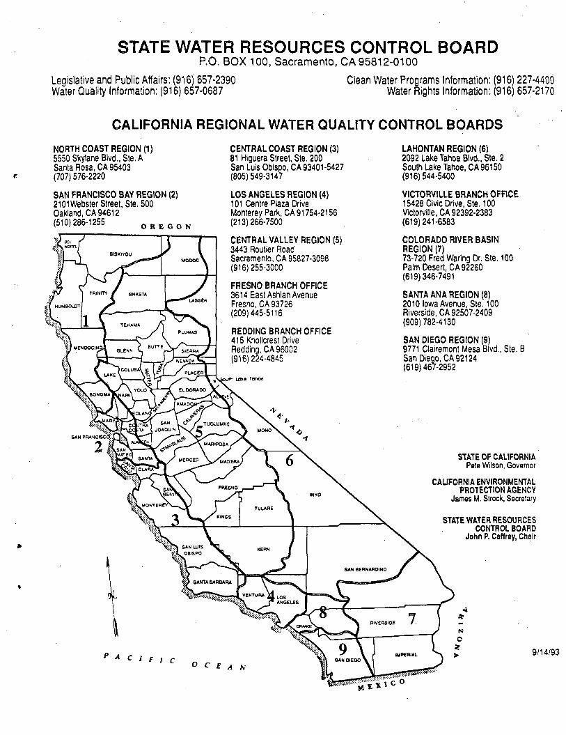
STATE WATER RESOURCES CONTROL BOARDP.O. BOX 100, Sacramento, CA 95812-0100

Legislative and Public Affairs: (916) 657·2390 Clean Water Programs Information: (916) 227·4406Water Quality Information: (916) 657·0687 Water Rights Information: (916) 657·2170

CALIFORNIA REGIONAL WATER QUALITY CONTROL BOARDS

SlAlE OF CALIFORNIAPete Wilson, Governor

STATE WATER RESOURCESCONTROL BOARD

John P. Caffrey, Chair

CAUFORNIA ENVIRONMENTALPROTECTION AGENCY

James M. Strock, Secretary

LAHONTAN REGION (6)2092 Lake Tahoe Blvd., Ste. 2South Lake Tahoe, CA96150(916) 544·5400

VICTORVILLE BRANCH OFFICE15428 Civic Drive, Ste. 100Victorville, CA 92392·2383(619) 241-6583

COLORADO RIVER BASINREGION (7)73-720 Fred Waring Dr. Ste. 100Palm Desert, CA 92260(619) 346-7491

SANTA ANA REGION (8)2010 Iowa Avenue, Ste.100Riverside, CA 92507-2409(909) 782·4130

SAN DIEGO REGION (9)9771 Clairemont Mesa Blvd., Ste. BSan Diego, CA92124 .(619) 467-2952

.Q

7 /If:RIVE~IOE

N

e~

9/'4/93>-

CENTRAL COAST REGION (3)81 Higuera Street, Ste. 200San Luis Obispo, CA 93401·5427(805) 549·3147

LOS ANGELES REGION (4)101 centre Plaza DriveMonterey Park, CA 91754·2156(213) 266·7500

CENTRAL VALLEY REGION (S)3443 Routier RoadSacramento, CA 95827·3098(916) 255·3000

FRESNO BRANCH OFFICE3614 East Ashlan AvenueFresno, CA 93726(209) 445·5116

REDDING BRANCH OFFICE415 Knollcrest DriveRedding, CA 96002(9'6) 224·4845

OREGON

NORTH COAST REGION (1)5550 Skylane Blvd., Ste. ASanta Rosa, CA 95403(707) 576·2220

SAN FRANCISCO BAY REGION (2)2101Webster Street, Ste. 500Oakland, CA 9461 2(510) 286·1255