1

Antitrust Analysis of Mergers with Bundling in Complementary Markets:

Implications for Pricing, Innovation, and Compatibility Choice

By

Jay Pil Choi*

September 2003

Abstract This paper develops a simple model to analyze the effects of mergers in

complementary system markets when the merged firm is able to engage in bundling. In the short-run analysis, I analyze the impact of (mixed) bundling on pricing decisions for existing generations of products. The basic model is then extended to analyze industry dynamics where the implications of mergers for innovation incentives and technical tying/compatibility decisions are explored. Welfare implications of mergers in the short- and long-run will be also analyzed.

Keywords: merger, mixed bundling, complementary markets, compatibility, innovation, and Cournot effect. Correspondent: Jay Pil Choi Department of Economics Michigan State University East Lansing, MI 48824 Tel: 517-353-7281 Fax: 517-432-1068 E-mail: choijay@msu.edu http://www.msu.edu/~choijay/

*I thank Zoltan Biro and Amelia Fletcher for useful discussions. This research is partially funded by the NET Institute whose financial support is gratefully acknowledged.

2

I. Introduction

On July 3, 2001, in one of its most high-profile antitrust decisions ever, the

European Commission blocked the proposed merger (valued at $43 billion) between

General Electric and Honeywell. Since it is the first case in which a proposed merger

between two U.S. companies that had been approved by Washington has been blocked by

European regulators, the decision has been closely scrutinized.1 One of the main issues

raised by the proposed GE/Honeywell merger concerned the possibility of “bundling” and

its likely impact on competition in the markets for jet aircraft engines and avionics.2 The

decision, however, has been criticized by many commentators for the alleged lack of sound

economic models to support.

This paper develops a model to analyze the effects of mergers in complementary

system markets when the merged firm is able to engage in bundling. The model builds on

the framework developed by Economides and Salop (1992). They analyze a model of

competition with complementary products in which they derive equilibrium prices for a

variety of organizational and market structures that differ in their degree of competition and

integration. However, they limit the strategy space of the merged entity and do not consider

the possibility of bundling which is made possible due to the merger.

There are essentially two forms of bundling in which the merged entity could

potentially engage:

� Under ‘mixed bundling’, the firm sells the individual components separately as well

as selling the bundle (but the bundle is offered at a discount to the sum of the stand-

alone prices).

� Under ‘pure bundling’, the firm only sells the bundle and it does not make the

individual components available separately.

1 As of this writing, the case is under appeal in the Court of First Instance of the European Union.

2 Another main issue that proved to be the stumbling block in the remedy negotiations between the merging parties and the Commission was the role and competitive implications of GECAS, GE’s aircraft leasing and financing arm.

3

The paper has two primary components – short-run and long-run analyses – since the form

of bundling undertaken by the merged entity might be expected to differ over time for the

following reasons:

� For existing generations of products, the potential for the merged firm to engage in

pure bundling may be limited.

� For new generations of products with R&D, one might expect the merged firm to

engage increasingly in pure bundling. This pure bundling could take the form of

‘technical tying’, whereby the merged firm would make its products available only as an

integrated system, making them incompatible with the individual components offered by

independent suppliers.

Much of the existing academic literature on bundling focuses on “pure bundling”

[see, for instance, Whinston (1990), Carbajo, de Meza, and Seidman (1990), and Choi and

Stefanadis (2001)].3 In the short-run, however, the merged entity, however, is expected to

engage in “mixed bundling,” continuing to sell the individual components separately but

selling them more cheaply as a bundle.4

Thus, this paper develops a model of mergers that allows mixed bundling. In

particular, I show that when the merging firms bundle their complementary products, the

short-run effects on pricing, market shares, and profits in the industry are as follows:

1. The merged firm will reduce the price of its bundled system and expand market share

relative to the situation prior to the merger. Prior to the merger, any price cut by one of the

merging firms will tend to benefit the other’s sales. In the absence of the merger, neither

party will take account of this benefit of a price cut on the other’s sales. Following the

merger, however, the merged entity can “internalize” these “pricing externalities” arising

3 In a model of strategic market foreclosure of tying, for instance, Whinston (1990) shows that mixed bundling is not a useful strategy. Thus, the motivation for mixed bundling is often found in the monopolistic bundling literature as a price discrimination device. See Adams and Yellen (1976) and McAfee, McMillan, and Whinston (1989).

4 As will be seen later, the incentive to practice mixed bundling rather than pure bundling in the short-run is confirmed in my model.

4

from the complementarity of their components by reducing the price of the bundle to below

the level the two players would choose if acting independently.5 This will expand the

merged firm’s sales and market share.

2. The merged firm will raise the prices of its stand-alone components, relative to their

levels prior to the merger. The merged firm has less to lose from raising its stand-alone

prices because a proportion of those customers that switch away from the stand-alone

components as a result of the price increase will simply switch to the bundle offered by the

merged firm rather than to the competing system. As such, the merged party will have an

increased incentive to set high prices for its components. This raises the price of “mix-and-

match” systems (i.e. systems including a component of the merged firm alongside a

competitor’s component) and makes them less attractive to buyers.

3. Independent rivals selling single components reduce their prices in response but fail to

recapture all market shares. In response to the price cut by the merged firm for their

bundled system and the price increase for the ‘mix-and-match' systems, the independent

rivals will cut price in order to retain some market share. However, they will not cut their

prices as much as the merged firm (i.e. their system will remain more expensive than the

bundled system of the merged firm) since – in the absence of counter-merger - they cannot

internalize the externality arising from the complementarity of their components. As a

result, they will fail to recapture all of their prior market shares. The merger would

therefore reduce the profits of the merged firm’s competitors. This reduction in profits

follows directly from the combination of a loss of market share and the need to cut prices.

Thus, there is a distinct possibility of exit by outside rival firms.

Bundling in my model entails both pro-competitive and anti-competitive effects.

There is no clear-cut answer to how mixed bundling by the merging parties would affect

consumer and social welfare. With heterogeneous consumer preferences, some buyers gain

5 Cournot (1838) is the first one to note that mergers among complements reduce prices. He considered the merger of two monopolists that produce complementary goods (zinc and copper) that are used as inputs for a final good (brass). My model extends his analysis to a case where both input producers face oligopolistic competition.

5

and others lose. For instance, those who previously purchased both products from the two

merging firms would gain due to the lower bundle price. However, those who continue to

purchase a mix and match system would suffer due to the increased stand-alone prices

charged by the merged firm. As a result, the overall impact on consumer and social welfare

is ambiguous. Numerical simulation results, however, suggest that the overall effects of

such a merger would be welfare-reducing if the substitution between systems were

sufficiently price-sensitive.

In the long-run analysis, I consider the effects of mergers on R&D incentives. It is

shown that the merging firms’ R&D incentives increase at the expense of the rival firms’.

The intuition for this result is the appropriability of the innovation benefit. Mergers with

bundling allow the merged entity to capture a larger market share in the systems market.

This implies that any cost reduction from an innovation translates into a larger profit with

merged firms. This leads to more aggressive R&D investment. For the same reason,

mergers with bundling dull the R&D incentives of outside rival firms. Finally, I also

consider the possibility of technical tying for new generations of products and show that it

can be an effective strategy for the exclusion of rivals.

The rest of the paper is organized in the following way. Section II sets up the basic

model and conducts a short-run analysis investigating the effects of mergers with mixed

bundling on pricing decisions. Section III deals with dynamic issues in the industry by

extending the model to allow for R&D opportunities and technical tying. Welfare

implications of mergers in the short- and long-run will be also analysed in sections 2 and 3,

respectively. Section IV concludes.

II. A Model of Mergers with Mixed Bundling

Consider two complementary components, A and B, which are valuable only when

used together. Customers combine A and B in fixed proportions on a one-to-one basis to

form a final product. For instance, I can consider A and B as operating systems and

application software, respectively, for computer, or cable/satellite service and content

providers, respectively, to provide entertainment. In the case of the proposed

6

GE/Honeywell merger, they correspond to engines and avionics, respectively, to form an

aircraft.

There are two differentiated brands of each of the two components A (A1 and A2)

and B (B1 and B2). Consequently, there are four ways to form a composite product, A1B1,

A1B2, A2B1, A2B2. Let the price of brand Ai be pi and the price of brand Bj be qj, where

i=1,2 and j=1,2. Then, the composite product AiBj is available at the total system price of sij

= pi + qj. Let Dij denote demand for the composite product AiBj. The combinations of

products and suppliers in this stylized model result in four possible systems, as shown in

Figure 1.

Figure 1: Diagrammatic representation of the pre-merger situation

As in Economides and Salop (1992), I assume that the four potential composite

goods are substitutes for one another: Dij is decreasing in its own price and increasing in the

prices of the three substitute composite goods. For instance, D11 is decreasing in s11, and

increasing in s12, s21, and s22. I can derive the demand functions for the components from

A1

A2

B1

B2

p 1

q 1

p 2

q 2

7

the demand functions for the composite goods. For instance, component Ai is sold as a part

of composite goods AiB1 and AiB2. Thus, the demand for component Ai is given by

DAi = Di1 + Di2

Similarly, the demand for component Bj is given by

DBj =D1j +D2j

I assume demand functions are linear and the demand system is symmetric:

D11(s11, s12, s21, s22 ) = a –b s11+ c s12+d s21+ e s22

D12(s12, s11, s22, s21 ) = a –b s12+ c s11+d s22+ e s21

D21(s21, s22, s11, s12 ) = a –b s21+ c s22+d s11+ e s12

D22(s22, s21, s12, s11 ) = a –b s22+ c s21+d s12+ e s11, where a, b, c, d, e>0.

I also assume that b> c+ d+ e to ensure that composite goods are gross substitutes, i.e., an

equal increase in the prices of all composite goods reduces the demand of each composite

good. To illustrate the effects of the merger, I further simplify the analysis by assuming that

all four composite products are equally substitutable, that is, c=d=e with the parameter

restriction of b>3c. Without loss of generality, I assume that constant unit production costs

are zero.6 The “a” parameter then represents the basic level of demand that would exist for

each system if the per unit margins on each system were zero. The “b” parameter describes

how demand for a given system falls as its own price increases (i.e. it reflects the own-price

elasticity of demand for that system). The “c” parameter describes how demand for a given

system rises as the prices of its competitors increase (i.e. it reflects the cross-price elasticity

of demand across systems). I now analyze how the market equilibrium changes depending

on the market structure.

II.1. Pre-merger situation

As a benchmark, I consider the case where all component brands Ai and Bj are

independently owned implying there are four separate firms. This case is analyzed in

Economides and Salop (1992) and describes the situation before a merger. Let p1, p2 , q1,

6 If there are positive constant unit production costs, the prices in the model can be interpreted as per unit margins.

8

and q2 denote the prices set by firms A1, A2, B1, and B2, respectively. Then I can write

each firm’s profit as:

ΠA1 = p1 (D11+D12); ΠA2 = p2 (D21+D22); ΠB1 = q1 (D11+D21); ΠB2 = q2 (D12+D22)

where:

D11 = a –b (p1 + q1 )+ c (p1 + q2 )+c (p2 + q1 )+ c (p2 + q2 )

D12 = a –b (p1 + q2 )+ c (p1 + q1 )+ c (p2 + q2 )+ c (p2 + q1 )

D21 = a –b (p2 + q1 )+ c (p2 + q2 )+ c (p1 + q1 )+ c (p1 + q2 )

D22 = a –b (p2 + q2 )+ c (p2 + q1 )+ c (p1 + q2 ) + c (p1 + q1 )

The market equilibrium (Nash equilibrium prices) is characterized by the following first-

order conditions:

∂ΠA1 /∂ p1 = 2a – 4(b - c) p1 + 4c p2 – (b - 3c) q1 – (b - 3c) q2 = 0

∂ΠB1 /∂ q1 = 2a – (b - 3c) p1 – (b - 3c) p2 – 4(b - c) q1 + 4c q2 = 0

∂ΠA2/∂ p2 = 2a + 4 c p1 – 4(b - c) p2 (b – 3c) q1 (b - 3c) q2 = 0

∂ΠB2/∂ q2 = 2a - (b - 3c) p1 – (b - 3c) p2 + 4 c q1 – 4(b - c) q2 = 0

The equilibrium prices under this regime ( Ip1 , Ip2 , Iq1 , Iq2 ), where superscript I denotes

Independent Ownership (i.e. the pre-merger situation)) are given as follows:

Ip1 = Ip2 = Iq1 = Iq2 =)73( cb

a−

Thus, the total system price of each composite good is given by:

sij = Iip + I

jq =)73(

2cb

a−

, where i, j = 1,2.

With the symmetry of the model, all four systems (A1B1, A1B2, A2B1, A2B2) have the same

market share of ¼ in the systems market by substituting the equilibrium prices back into the

demand function:

D11 = D12 = D21 = D22 = 2

2 2( )

3 9 4a b c

b bc c−

− +

Thus, each firm has the same market share of ½ with demand of 2

2 22 ( )

3 9 4a b c

b bc c−

− +in the

relevant stand-alone markets. Each firm’s profit in turn can be derived as:

9

ΠA1 = ΠA2 = ΠB1 = ΠB2 = 2

22 ( )(3 7 )a b cb c

−−

II.2. Merger between A1 and B1 with Mixed Bundling

Now suppose that A1 and B1 merge. As a merged entity, A1-B1 can offer three

prices, s for the bundled product (A1B1) and 1~p and 1

~q for individual components A1 and

B1, respectively. A2 and B2 remain independent and charge prices 2~p and 2

~q , respectively.

Figure 2 describes the post-merger situation with mixed bundling.

Figure 2: Diagrammatic representation of post -merger with mixed bundling

( Ip1 < 1~p )

( Ip1 + Ip2

>s)

A1

B1

B2

A2

( Iq1 < 1~q ) ( Iq2 > 2

~q )

( Ip2 > 2~p )

B1

A1

Then, the profit functions for the merged firm (A1-B1) and independent firms (A2

and B2) are respectively given by

ΠA1 –B1= sD11 + p1 D12 + q1 D21

ΠA2 = p2 (D21 + D22) and ΠB2= q2 (D12 + D22) , where

D11 = a –b s+ c (p1 + q2)+c (p2 + q1 )+ c (p2 + q2)

D12 = a –b (p1 + q2)+ c s+ c (p2 + q2)+ c (p2 + q1)

D21 = a –b (p2 + q1)+ c (p2 + q2)+ c s+ c (p1 + q2)

D22 = a –b (p2 + q2)+ c (p2 + q1)+ c (p1 + q2) + c s

10

The merged firm’s profit, ΠA1 –B1, consists of three components: the profit from selling the

bundle A1B1 ( sD11), the profit from selling stand-alone product A1 as part of the mix-and-

match system A1B2 (p1 D12), and the profit from selling stand-alone product B1 as part of the

mix-and-match system A2B1 (q1 D21).

The market equilibrium (Nash equilibrium prices) is characterized by the following

first-order conditions:

∂ΠA1 –B1/∂s = a – 2 b s + 2c p1 + 2 c p2 + 2c q1 +2c q2 = 0

∂ΠA1 –B1/∂ p1 = a + 2 c s – 2b p1 + 2 c p2 + 2c q1 – (b - c) q2 = 0

∂ΠA1 –B1/∂ q1 = a + 2 c s + 2c p1 – (b - c) p2 – 2b q1 + 2c q2 = 0

∂ΠA2/∂ p2 = 2a + 2 c s + 2c p1 – 4(b - c) p2 – (b - c) q1 (b - 3c) q2 = 0

∂ΠB2/∂ q2 = 2a + 2 c s – (b - c) p1 – (b - 3c) p2 + 2 c q1 - 4(b - c) q2 = 0

By taking advantage of the symmetry of the model, I can derive the equilibrium market

prices as 1~p = 1

~q = x, and 2~p = 2

~q =y, where x and y satisfy

a – 2 b s + 4c (x+y) = 0

a + 2 c s – 2(b – c) x – (b - 3c) y = 0

2 a + 2 c s – (b - 3c) x – (5b - 7c )y = 0

Solving the equations above simultaneously yields:

)493(2)3(~

22 cbcbcbas+−

−= (the bundle price)

1~p = 1

~q = 22 493 cbcbab

+− (stand-alone product price by the merged firm)

2~p = 2

~q = 22 493)(

cbcbcba+−

− (independent firms’ component price)

With the parameter restriction b>3c, I have the following result.

Proposition 1. The model shows that mixed bundling following the merger would have the

following implications for prices.

11

� First, the price of the bundle post-merger is lower than the sum of the pre-merger

component prices ()493(2

)3(~22 cbcb

cbas+−

−= < Iijs = I

ip + Ijq =

cba73

2−

).7

� Second, the merged firm’s prices for individual components are higher with mixed

bundling ( 1~p = 1

~q = 22 493 cbcbab

+−> Ip1 = Iq1 =

cba

73 −)

� Third, the independent firms also cut their prices ( 2~p = 2

~q = 22 493)(

cbcbcba+−

−

< Ip2 = Iq2 =cb

a73 −

).

With the equilibrium prices derived for mixed bundling, I can calculate the changes in

market shares and profits after the merger. The demand for each system after the merger is

given by:

�D 11 = 2 2(3 5 )

2(3 9 4 )ab b cb bc c

−− +

�D 12 = �D 21 = 2 2

2 2(2 5 )

2(3 9 4 )a b bc c

b bc c− +

− +

�D 22 =2 2

2 2(2 3 3 )

2(3 9 4 )a b bc c

b bc c− +− +

The profits of the merged firm and outside firms are given by:

�Π A1-B1 = 2 2 2

2 2 2(17 38 9 )

4(3 9 4 )a b b bc c

b bc c− +

− +

�Π A2 = �Π B2 =2 3

2 2 22 ( )

(3 9 4 )a b c

b bc c−

− +

7 This can be easily proved with our assumption of the gross substitutability of the demand systems, that is, b>3c.

12

Proposition 2. Mixed bundling following the merger would have the following implications

for market shares and profits.

� First, the demands for the bundle (A1B1) and the system comprised of outside firms’

components (A2B2) increase at the expense of mix-and-match systems (A1B2 and

A2B1 ). Since the bundle price is lower than the sum of the outside firms’ component

prices, the increase in the demand for the bundle is larger than that for the outside

system, that is, �D 11 > �D 22 > (Dij) > �D 12 = �D 21.

� Second, the derived demand for the components increases for the merging firms at

the expense of the derived demand for outside firms ( �D 11+ �D 12 = �D 11+ �D 21 > D11 +

D12 =D11 + D21 , �D 21 + �D 22 = �D 12 + �D 22 < D21 + D22 =D12 + D22).

� Third, the merging firms’ profits increase at the expense of independent firms’

profits ( �Π A1-B1 > ΠA1 + ΠB2 , �Π A2 = �Π B2 < ΠA2 = ΠB2 ). The merger would

therefore reduce the profits of the merged firm’s competitors. This reduction in

profits follows directly from the combination of a loss of market share and the need

to cut prices. 8

Example. Consider the case where a=b=1 and c=1/4. Then I can show that with the

independent ownership (pre-merger) structure, Ip1 = Ip2 = Iq1 = Iq2 =4/5. The total price of

each composite good is 8/5 and each firm gets the profits of 24/25.

After the merger between A1 and B1, the merged entity (A1-B1) charges s� =11/8 for

the bundle and 1~p = 1

~q =1 for separate components. Thus, it offers discount for the

bundle (11/8 < 1+1=2). Independent producers, A2 and B2, charge 2~p = 2

~q = ¾ for their

component products. Thus, the prices for composite products, A1B1, A1B2, A2B1, and A2B2

8 All results can be easily proved algebraically by simple manipulations with the assumption of b>3c, except the merging firms’ profit changes. The Mathematica program, however, shows that the merging firms’ profits increase after the merger.

13

are given by 11/8, 7/4, 7/4, and 3/2, respectively, where 7/4>3/2>11/8. After the merger

A1-B1 receives the profits of 129/64 (>24/25+24/25), whereas independent producers get

27/32 (<24/25). This implies that A1 and B1 together increase their combined profits after

merger while independent producers’ profits decrease.

II.3. Welfare Analysis

I perform a welfare analysis of the effects of a merger in the absence of foreclosure.

I take the sum of consumer and producer surplus as a measure of social welfare. To derive

the consumer surplus, I first invert the demand system to obtain inverse demand functions

(that is, demand functions in which the price of a system is given as a function of sales

volumes for all systems). The inverse demand system can be written as:

s11 (D11, D12

, D21, D22) = (β+γ) a – (β−2γ)D11– γ D12

– γ D21 – γ D22

s12 (D11, D12

, D21, D22) = (β+γ) a – γ D11– (β−2γ)D12

– γ D21 – γ D22

s21 (D11, D12

, D21, D22) = (β+γ) a – γ D11– γ D12

–(β−2γ) D21 – γ D22

s22 (D11, D12

, D21, D22) = (β+γ) a – γ D11– γ D12

– γ D21 – (β−2γ)D22

,

where β=

))(3( cbcbb

+−and γ=

))(3( cbcbc

+−.

These inverse demand functions imply that the utility function is given by:

U(D11, D12

, D21, D22) = (β+γ) a [D11

+ D12 + D21

+ D22] −

22γβ − [

211( )D + 212( )D +

221( )D + 222( )D ] – γ [ D11 D12 + D11 D21 + D11 D22 + D12 D21 + D12 D22 + D21 D22

]

Having calculated this utility function, it is possible to calculate total consumer valuations of

the products purchased.

In my linear model, the level of the demand intercept “a” has no effect on the relative

prices. Similarly, the parameters b and c only affect the results through the ratio of b/c. I

14

thus normalize a = b =1 and analyze the effects of a merger on social welfare as I change the

c parameter. With the assumption of the gross substitutability of composite goods, the

normalization of b=1 implies that c∈ (0, 1/3). With these restrictions, I can calculate pre-

merger social welfare, W, and post-merger social welfare, W~ , as follows:

W = )31()73()13185(2

2

2

cccc

−−+− , W~ = 22

432

)493)(31(88842174145587

ccccccc

+−−+−+−

I plot the changes in social welfare due to the merger in Figure 3.

222

5432

)493()37(832814713152227464863~

ccccccccWW

+−−−+−+−=−

)13185()493(16)8842174145587()73(~

222

4322

ccccccccc

WW

+−+−+−+−−=

Figure 3. Absolute Changes and the Ratio of Social Welfare due to a Merger

15

I emphasize that the above calculations assume there is no foreclosure due to the

merger and the merging firm does not behave strategically with anticompetitive intent.

Otherwise, the effects of a merger on social welfare would be decidedly negative. For

instance, suppose that there is a fixed cost of operation F that can be avoided by exiting the

industry. If I have a situation such that �Π A2 = �Π B2 < F <ΠA2 = ΠB2, a merger between A1

and B1 will induce exit by the outsiders, and social welfare will be unambiguously affected

in a negative way.

Even in the absence of such foreclosure effects, there could be significant welfare

loss when c (cross-substitutability parameter) is sufficiently large. When c is close to zero,

each system is essentially a separate product, and there is little direct competition between

systems. In this case, the structure of each system market is equivalent to the one

considered by Cournot and mergers are welfare enhancing. In cases with high degrees of

substitutability and intense competition among systems (i.e., high c), however, the model

suggests that the effects of mergers on social welfare are negative.

III. The Effects of Mergers on the R&D Incentives Compatibility Decision

In the previous section, I have analyzed the effects of mergers on pricing assuming

that the product characteristics and cost structures are given. I now extend the basic

framework laid out in section II to analyze the impact of mergers on R&D incentives and

incentives to engage in pure bundling when technical tying is feasible as a result of the

merger. To this end, I consider a two-stage game in which price competition is preceded by

R&D competition/ compatibility decision. The basic model indicates that bundling (or

incompatible product design) on the part of the merged firm reduces the future market

available to independent rivals and consequently reduces their incentives to invest in cost

reducing R&D. The main intuition is that firms’ incentives to engage in R&D activities are

proportional to their outputs in the product market since R&D costs are largely sunk (Choi,

forthcoming). Any reduction in the future market available will thus reduce expected future

profits and current R&D spending. The analysis of the incentives to bundle can also be

16

applied to the compatibility decision for the merged firm with the rest of the suppliers since

pure bundling is the same as the choice of incompatibility in its economic effects.

III.1. The Effects of Mergers (with Mixed Bundling) on R&D Incentives

This subsection describes how the reduced output by independent firms due to the A1-B1

merger will adversely affect independent firms’ R&D incentives.

Let me denote A1, A2, B1, and B2’s marginal costs as α1, α 2, β1, and β 2, respectively.

Let

γγγγ = ( α1, α 2 , β1, β 2 ) be the vector of marginal costs. Then I can represent each firm’s

equilibrium profits in the pre-merger situation as:

));(),(),(),(( 21211 γγγγγ qqppAΠ

));(),(),(),(( 21212 γγγγγ qqppAΠ

));(),(),(),(( 21211 γγγγγ qqppBΠ

));(),(),(),(( 21212 γγγγγ qqppBΠ ,

where )(1 γp , )(2 γp , )(1 γq , and )(2 γq are equilibrium prices for A1, A2, B1, and B2 when

γγγγ is the industry cost structure.

Prior to the merger between A1 and B1, the R&D incentives for A2 can be represented by:

2 2 2 2 2 21 2 1 2

2 2 1 2 2 2 1 2 2 2

A A A A A Ad p p q qd p p q qα α α α α α

Π ∂Π ∂Π ∂ ∂Π ∂ ∂Π ∂ ∂Π ∂− = − + + + + ∂ ∂ ∂ ∂ ∂ ∂ ∂ ∂ ∂

The expression above yields the marginal benefit to A2 from decreasing its production cost

and thus represents the R&D incentives for A2. By the envelope theorem:

2

2

A

α∂Π∂

= − (D21+D22)

which is the equilibrium output level for A2 prior to innovation, and

17

2

2

A

p∂Π∂

= 0.

Therefore, I can rewrite the expression for A2’s R&D incentives as:

2 2 2 221 22 1 1 2

2 1 2 1 2 2 2( )

A A A Ad p q qD Dd p q qα α α α

Π ∂Π ∂ ∂Π ∂ ∂Π ∂− = + − + + ∂ ∂ ∂ ∂ ∂ ∂

I can interpret the term (D21+D22) as the direct effects of innovation through cost saving and

the second term:

2 2 21 1 2

1 2 1 2 2 2

A A Ap q qp q qα α α

∂Π ∂ ∂Π ∂ ∂Π ∂− + + ∂ ∂ ∂ ∂ ∂ ∂

as the indirect effects of innovation through price competition.

After the A1-B1 merger, I can represent each firm’s equilibrium profits in the pre-merger

situation as:

));(~),(~),(~),(~),(~(~2121

11 γγγγγγ qqppsBA −Π

));(~),(~),(~),(~),(~(~2121

1 γγγγγγ qqppsBΠ

));(~),(~),(~),(~),(~(~2121

2 γγγγγγ qqppsBΠ ,

where )(~ γs is the bundle price, and other variables corresponding with the post merger

situation are denoted with a tilde. Then the post-merger expression for A2’s R&D

incentives can be written as:

2 2 2 2 2 2 21 2 1 2

2 2 2 1 2 2 2 1 2 2 2

A A A A A A Ad s p p q qd s p p q qα α α α α α α

Π ∂Π ∂Π ∂ ∂Π ∂ ∂Π ∂ ∂Π ∂ ∂Π ∂− = − + + + + + ∂ ∂ ∂ ∂ ∂ ∂ ∂ ∂ ∂ ∂ ∂

� � � � � � �� � � � �

� � � � �

Once again, by the envelope theorem,

18

2

2

AddαΠ� = −( 21~D + 22~D ),

which is the post-merger equilibrium output level for A2 prior to innovation, and

2

2

A

p∂Π∂

�

�= 0.

Therefore, I can rewrite the expression for A2’s R&D incentives as:

2 2 2 2 221 22 1 1 2

2 2 1 2 1 2 2 2( )

A A A A Ad s p q qD Dd s p q qα α α α α

Π ∂Π ∂ ∂Π ∂ ∂Π ∂ ∂Π ∂− = + − + + + ∂ ∂ ∂ ∂ ∂ ∂ ∂ ∂

� � � � �� � � �� �

� � � �

Once again, I can interpret the first term −( 21~D + 22~D ) as the direct effects and the second

term

2 2 2 21 1 2

2 1 2 1 2 2 2

A A A As p q qs p q qα α α α

∂Π ∂ ∂Π ∂ ∂Π ∂ ∂Π ∂− + + + ∂ ∂ ∂ ∂ ∂ ∂ ∂ ∂

� � � �� � � �

� � � �

as the indirect effects.

If I compare the direct effects of innovation, A2 will unambiguously reduce R&D

expenditures since its market output contracts after the A1-B1 merger; (D21+D22)

> ( 21~D + 22~D ).

In general, the indirect effects of innovation through price competition before and after the

merger are not directly comparable. However, if the merged firm responds more

aggressively to other firms’ price cuts after the merger, I expect that:

2 2 2 2

1 1 2

2 1 2 1 2 2 2

A A A As p q qs p q qα α α α

∂Π ∂ ∂Π ∂ ∂Π ∂ ∂Π ∂− + + + ∂ ∂ ∂ ∂ ∂ ∂ ∂ ∂

� � � �� � � �

� � � �

is smaller than

19

2 2 2

1 1 2

1 2 1 2 2 2

A A Ap q qp q qα α α

∂Π ∂ ∂Π ∂ ∂Π ∂− + + ∂ ∂ ∂ ∂ ∂ ∂ .

Then A2 will unambiguously reduce its R&D. Even if the last inequality is reversed, if the

direct effects of innovation are sufficiently large compared to the indirect effects, A2 will

still reduce its R&D.

In the Appendix, I conduct a simulation analysis in which I confirm that the merged

firm increases its R&D level whereas outside rival firms reduce their R&D levels in a linear

demand model with quadratic R&D cost functions. I also perform a dynamic welfare

analysis and show that the effects of mergers can be especially harmful in industries with

more R&D opportunities.

III.2. Pure Bundling/Compatibility Choice and Foreclosure

Until now, I have analyzed only the possibility of mixed bundling after a merger

between complementary producers in which the merged firm sells the individual

components separately as well as selling the bundle (but the bundle is offered at a discount

to the sum of the stand-alone prices). In this subsection, I consider another type of practice

known as pure bundling, under which the firm only sells the bundle and does not make the

individual components available individually. For existing generations of products, it is a

reasonable assumption that the merged firm’s ability to engage in pure bundling is limited

since pure bundling is typically not an ex post optimal strategy for the merged firm, and thus

it requires a commitment device. 9

In the long run, however, the merged firm can commit to pure bundling in the form

of technical tying, especially for new generations of products, by making its products

available only as an integrated system, incompatible with the individual components offered

by outside suppliers. In such a case, the only available systems in the market are A1-B1 and

9 See Whinston (1990) for a classical analysis of pure bundling in which he shows the importance of commitment ability for bundling to have any impact on competition.

20

A2-B2 since A1 and B1 will only function effectively as part of the bundled system and

cannot be used alongside components from other suppliers. By inverting the inverse

demand system in section II.3 with the constraint D12 = D21

= 0, I can derive the following

demand system:

D11(s, p2, q2 ) =( )( )b cb c

+− 2 2[ ( 2 )( ) ]a b c p q cs− − + +

D22(s, p2, q2 ) =( )( )b cb c

+− 2 2[ ( 2 )( ) ]a b c p q cs− − + + ,

where s = the merged firm’s price for system A1-B1 , 2p = the price of A2 and

2q =the price of B2.

Then the profit functions for the merged firm (A1-B1) and independent firms (A2 and B2)

with pure bundling are respectively given by

ΠA1 –B1= sD11 , ΠA2 = p2 D22 and ΠB2= q2 D22

The market equilibrium (Nash equilibrium prices) is characterized by the following first-

order conditions:∂ΠA1 –B1/∂s = 0,∂ΠA2/∂ p2 = 0, and∂ΠB2/∂ q2 = 0. Solving the conditions

simultaneously yields:

2 2(3 4 )

2(3 12 11 )a b cs

b bc c−=

− + (the bundle price)

2p = 2q = 2 2(2 3 )

2(3 12 11 )a b c

b bc c−

− + (independent firms’ component price)

As in the case of mixed bundling, the bundle price offered by the merged firm is lower than

the sum of independent firms’ component prices. As a result, the merged firm dominates the

outside firms in terms of market share.

I conduct a numerical analysis to investigate the profitability of mergering with pure

bundling. Once again, I normalize parameters with a=b=1. With this normalization, the

effects of a merger with pure bundling on the merging and outside firms’ profits are plotted

in Figures 4 and 5.

21

1 1A B−Π 1 1( )A B− Π + Π

0.05 0.1 0.15 0.2 0.25 0.3

1

2

3

4

5

6

b

1 1A B−Π = merged entity’s profit with pure bundling

1AΠ = pre-merger profit for firm A1

1BΠ = pre-merger profit for firm B1

Figure 4. Changes in Profits for the Merging Firms with Pure Bundling

2AΠ − 2AΠ and

2BΠ − 2BΠ

0.05 0.1 0.15 0.2 0.25 0.3

-0.2

-0.1

0.1

2AΠ ,

2BΠ = post-merger profits for outsiders with pure bundling

2AΠ , 2BΠ = pre-merger profits for firms A2 and B2, respectively

Figure 5. Changes in Profits for the Outsiders with Pure Bundling

22

Thus, the merger with pure bundling is profitable for merging firms A1 and B1. However,

pure bundling is less profitable than mixed bundling for the merged entity as shown in

Figure 6.

1 1A B−Π −�

1 1A B−Π

0.05 0.1 0.15 0.2 0.25 0.3

-0.3

-0.2

-0.1

0.1

1 1A B−Π = merged entity’s profit with pure bundling

�1 1A B−

Π = merged entity’s profit with mixed bundling

Figure 6. Mergers with Pure Bundling vs. Mixed Bundling

I can thus conclude that the merged firm will not practice pure bundling since mixed

bundling yields higher profits as an accommodation strategy. However, as in Whinston

(1990), pure bundling can be still profitable if the exclusion of rivals through predation is

possible with pure bundling, but not with mixed bundling. This may occur because

outsiders’ profits are affected more adversely with pure bundling. To see this, I plot the

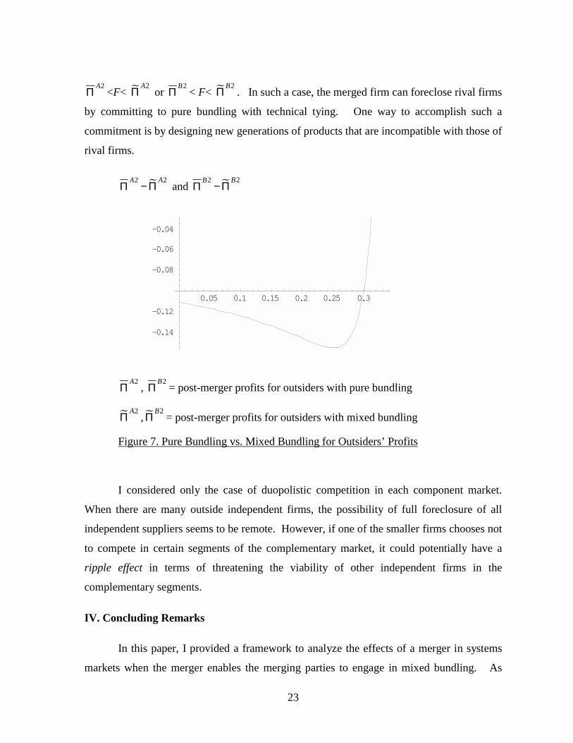
differences in outsiders’ profits with pure bundling and mixed bundling in Figure 7.10

Thus, I can imagine a situation where there is a fixed cost of operation and rival

firms can recoup fixed costs with mixed bundling but not with pure bundling, that is,

10 For the sake of brevity, I report only the effects of pure bundling with price competition. However, similar results can be derived when we introduce the possibility of R&D competition in the model.

23

2AΠ <F< �

2AΠ or

2BΠ < F< �

2BΠ . In such a case, the merged firm can foreclose rival firms

by committing to pure bundling with technical tying. One way to accomplish such a

commitment is by designing new generations of products that are incompatible with those of

rival firms.

2AΠ −�

2AΠ and

2BΠ −�

2BΠ

0.05 0.1 0.15 0.2 0.25 0.3

-0.14

-0.12

-0.08

-0.06

-0.04

2AΠ ,

2BΠ = post-merger profits for outsiders with pure bundling

�2A

Π , �2B

Π = post-merger profits for outsiders with mixed bundling

Figure 7. Pure Bundling vs. Mixed Bundling for Outsiders’ Profits

I considered only the case of duopolistic competition in each component market.

When there are many outside independent firms, the possibility of full foreclosure of all

independent suppliers seems to be remote. However, if one of the smaller firms chooses not

to compete in certain segments of the complementary market, it could potentially have a

ripple effect in terms of threatening the viability of other independent firms in the

complementary segments.

IV. Concluding Remarks

In this paper, I provided a framework to analyze the effects of a merger in systems

markets when the merger enables the merging parties to engage in mixed bundling. As

24

such, it can shed some light on merger/divestiture issues in network industries such as

“portfolio effects” or “range effects.” The model, for instance, can be applied to the recent

proposed merger between GE and Honeywell. When the European Commission blocked

the proposed merger, the decision was heavily, and in my opinion unfairly, criticized in the

popular press and by the U.S. antitrust agencies and senior administration officials, raising

fears of escalating trade disputes between the US and EU.11 In particular, there have been

some unfortunate suggestions in the newspapers that the decision was made without any

theoretical support.12 This paper, in contrast, shows that the effects of bundling can be

analyzed with sound economic modeling.

My model suggests that mergers with bundling in systems markets could entail both

pro-competitive and anti-competitive effects. In the event of any foreclosure of competitors,

however, conglomerate mergers with mixed bundling would be predominantly anti-

competitive. Even in the absence of such foreclosure effects, there is no clear-cut answer to

how mixed bundling by the merging parties would affect consumer and social welfare.

With heterogeneous consumer preferences, some buyers gain and others lose. For instance,

those who previously purchased both products from the two merging firms would gain due

to the lower bundle price. However, those who continue to purchase a mix-and-match

system would suffer due to the increased stand-alone prices charged by the merged firm. As

a result, the overall impact on consumer and social welfare is ambiguous. In general,

conglomerate mergers would have different implications for competition depending on

specific market conditions such as market shares of the merging parties in their individual

markets, economies of scale due to avoidable fixed costs, ease of entry, etc. To sort out pro-

competitive effects and anti-competitive effects of each conglomerate merger case, the

relative magnitudes of these countervailing effects and the likelihood of the foreclosure of

11 See, for instance, the address by William J. Kolasky (2001), Deputy Assistant Attorney General for International Affairs in the Antitrust Division of the U.S. Department of Justice.

12 Interestingly enough, the EC’s bundling theory was described as “19th-century thinking” in the New York Times whereas it was described as “novel” in the Wall Street Journal. See Hal R. Varian, Economic Scene; In Europe, GE and Honeywell ran afoul of 19th-century thinking.," N.Y. Times, June 28, 2001 and Editorial, Europe to GE: Go Home, Wall Street J., June 15, 2001.

25

one or more competitors need to be assessed. Blanket approvals of conglomerate mergers

with the presumption that bundling is either pro-competitive or competitively neutral are

certainly not warranted.

26

References

Adams, William, J. and Yellen, Janet L., “Commodity Bundling and the Burden of Monopoly”, Quarterly Journal of Economics, 90, August 1976, p. 475-498.

Carbajo, Jose, De Meza, David and Seidman, Daniel J., "A Strategic Motivation for Commodity Bundling," Journal of Industrial Economics, March 1990, 38, pp. 283-298.

Choi, Jay P., “Preemptive R&D, Rent Dissipation, and the Leverage Theory,” Quarterly Journal of Economics, 1996, pp. 1153-1181.

Choi, Jay. P., “Tying and Innovation: A Dynamic Analysis of Tying Arrangements,” Economic Journal, forthcoming.

Choi, Jay P. and Stefanadis, Chris, “Tying, Investment, and the Dynamic Leverage Theory”, Rand Journal of Economics, 2001, pp. 52-71.

Cournot, Augustine, “Researches into the Mathematical Principles of the Theory of Wealth”, originally published in French (1838), translated by Nathaniel Bacon, New York: Macmillan, 1927.

Economides, Nicholas and Salop, Steven C., “Competition and Integration among Complements, and Network Market Structure,” Journal of Industrial Economics, XL, 1992, pp. 105-123.

Kolasky, William, J. “Conglomerate Mergers and Range Effects: It's a Long Way From Chicago to Brussels,” Address before the George Mason University Symposium, Washington, DC, November 9, 2001. Available at http://www.usdoj.gov/atr/public/speeches/9536.htm.

Matutes, Carmen and Regibeau, Pierre, “Mix and Match: Product Compatibility Without Network Externalities,” Rand Journal of Economics, 1988, pp. 221-234.

McAfee, Preston R., McMillan, John and Whinston, Michael D., “Multiproduct Monopoly, Commodity Bundling, and Correlation of Values”, Quarterly Journal of Economics, 104, May 1989, pp. 371-384.

Whinston, Michael D., “Tying, Foreclosure, and Exclusion”, American Economic Review, Vol. 80, No. 4, 1990, pp.

27

Appendix. The Effects of Merger with Mixed Bundling on R&D Incentives

In this appendix, I conduct a simulation analysis on the effects of mergers on R&D

incentives and welfare implications in a linear demand model with a quadratic R&D cost

function. For the sake of presentation, I consider R&D that improves the quality of

components and shifts the system demand curves outward. More precisely, let ( 1∆ , 2∆ ,

1δ , 2δ ) denote quality improvements of components A1, A2, B1, B2, respectively, which

represent consumers’ willingness to pay for the systems that contain them. For instance,

consumers’ willingness to pay for the system AiBj increases by i∆ + jδ . Let me assume

that the cost of improving the quality of each component is given by k 2∆ /2, where ∆ is the

amount of quality improvement and k is an R&D cost parameter.

The inverse demand system can be written as:

s11 (D11, D12

, D21, D22) = (β+γ) a + ( 1∆ + 1δ ) – (β−2γ)D11– γ D12

– γ D21 – γ D22

s12 (D11, D12

, D21, D22) = (β+γ) a + ( 1∆ + 2δ ) – γ D11– (β−2γ)D12

– γ D21 – γ D22

s21 (D11, D12

, D21, D22) = (β+γ) a + ( 2∆ + 1δ ) – γ D11– γ D12

–(β−2γ) D21 – γ D22

s22 (D11, D12

, D21, D22) = (β+γ) a + ( 2∆ + 2δ )– γ D11– γ D12

– γ D21 – (β−2γ)D22

,

where β=

))(3( cbcbb

+−and γ=

))(3( cbcbc

+−.

Then, the inverse demand system implies the following system demand functions given

( 1∆ , 2∆ , 1δ , 2δ ):

D11 = a + (b−c) ( 1∆ + 1δ ) –2c( 2∆ + 2δ ) –b (p1 + q1 )+ c (p1 + q2 )+c (p2 + q1 )+ c (p2 + q2 )

D12 = a + (b−c) ( 1∆ + 2δ ) –2c( 2∆ + 1δ ) –b (p1 + q2 )+ c (p1 + q1 )+ c (p2 + q2 )+ c (p2 + q1 )

D21 = a + (b−c) ( 2∆ + 1δ ) –2c( 1∆ + 2δ ) –b (p2 + q1 )+ c (p2 + q2 )+ c (p1 + q1 )+ c (p1 + q2 )

28

D22 = a + (b−c) ( 2∆ + 2δ ) –2c( 1∆ + 1δ )–b (p2 + q2 )+ c (p2 + q1 )+ c (p1 + q2 ) + c (p1 + q1 )

For a simulation analysis, let me normalize the parameters to a=b=1. Then, Figures

A-1 and A-2 show the changes in profits due to the A1-B1 merger for the merging firms (A1

and B1) and outsider firms (A2 and B2) for parameter values k ∈ [20,100] and c∈ [0,1/3].

0

0.1

0.2

0.3 20

40

60

80

100

0

0.005

0.01

0.015

0

0.1

0.2

0.3

Figure A-1. Changes in Profits for the Merging Firms with R&D

0

0.1

0.2

0.3 20

40

60

80

100

-0.004

-0.002

0

0

0.1

0.2

0.3

Figure A-2. Changes in Profits for the Outsider Firms with R&D

29

Our simulation results suggest that for wide ranges of parameter spaces, the merger is

profitable for A1 and B1 whereas it reduces the outsider firms’ profits. Welfare implications

of the merger in the presence of R&D are represented in Figure A-3.

0

0.1

0.2

0.3 20

40

60

80

100

-0.3-0.2-0.1

00.1

0

0.1

0.2

0.3

Figure A-2. Changes in Welfare due to Mergers in the Presence of R&D

As in the case without R&D, simulation results suggest that welfare results are

ambiguous and depend crucially on c (cross-substitutability parameter). Once again, when c

is close to zero, each system is essentially a separate product and there is little direct

competition between systems. In this case, the structure of each system market is equivalent

to the one considered by Cournot and the merger is welfare enhancing. In cases with high

degrees of substitutability and intense competition among systems, the effects of mergers on

social welfare are negative.

To investigate the effects of the R&D cost parameter, I also plot the changes in

welfare due to mergers with three different values of k in Figure A-3. The results suggest

that mergers are more likely to reduce welfare when there are more opportunities for cost

reduction through R&D, that is, when k is lower.

30

�W W−

0.05 0.1 0.15 0.2 0.25

-2

-1.5

-1

-0.5

for k=20

�W W−

0.05 0.1 0.15 0.2 0.25

-0.6

-0.4

-0.2

for k=50

�W W−

0.05 0.1 0.15 0.2 0.25

-0.4

-0.3

-0.2

-0.1

0.1

for k=100

Figure A-3. The Effects of R&D Opportunities on Changes in Welfare due to Mergers