The Welfare Effects of Bundling in Multichannel

Television Markets ∗

Gregory S. Crawford† Ali Yurukoglu‡

July 2010

Abstract

We measure how the bundling of television channels affects social welfare. We estimate an

industry model of viewership, demand, pricing, bundling, and input market bargaining using

data on ratings, purchases, prices, bundle composition, and aggregate input costs. We conduct

counterfactual simulations of à la carte policies that require distributors to offer individual chan-

nels for sale to consumers. We estimate that input costs riseby 145.2% in equilibrium under à

la carte. These are passed on as higher prices, offsetting consumer surplus benefits from pur-

chasing individual channels. Before any implementation and marketing costs, mean consumer,

producer, and total surplus change by an estimated -1.0%, 13.0%, and 5.3%.

∗We would like to thank Dan Ackerberg, Derek Baine, Lanier Benkard, Liran Einav, Catherine de Fonte-nay, Philip Leslie, Alessandro Pavan, David Pearce, Amil Petrin, Peter Reiss, Paulo Somaini, Alan Sorensen,Steve Stern, John Thanassoulis, Tracy Waldon, and seminar participants at numerous universities and con-ferences. We especially thank Yurukoglu’s dissertation advisers Ariel Pakes, Luis Cabral, John Asker, andAllan Collard-Wexler. Robin Lee’s collaboration on another project helped us to improve several aspects ofthe paper.

†Department of Economics, University of Warwick‡Graduate School of Business, Stanford University

1

1 Introduction

Bundling is widespread in multichannel television markets.1 In theory, bundling can be a profitable

form of price discrimination. It makes consumer tastes morehomogenous which facilitates surplus

extraction, but it has ambiguous effects on total welfare (Stigler (1963), Adams and Yellen (1976),

McAfee, McMillan and Whinston (1989)). Regulations mandatingà la cartepricing would radically

alter the choice sets of the roughly 110 million U.S. television households who collectively spend

more than $50 billion annually and watch an average of more than seven hours of television per day.

This paper predicts the impact of such a regulation on the distribution of consumer and producer

welfare.

There are widely differing opinions among policy makers, consumers, and industry participants

about the effects of mandating à la carte pricing in the U.S.2 This lack of consensus is partly because

regulations mandating unbundling have not been implemented in enough similar circumstances to

provide direct evidence.3 Experimentation is impractical as unbundling would changenot only

outcomes at the retail level, but also industry-wide negotiations between content providers and dis-

tributors.4 We develop a model to evaluate à la carte pricing.

We model viewership, demand, pricing, bundling, and input market bargaining of multichannel

television services. We estimate the distribution of household preferences for almost fifty cable

television channels using ratings and bundle market share data. We estimate the input costs that

distributors, such as Comcast and DirecTV, currently pay tocontent providers, such as ESPN and

CNN, using aggregate cost data and observed pricing and bundling decisions. We use the demand

and cost estimates to estimate the parameters of a bilateralbargaining with externalities model of the

input market. Finally, we hold the estimated demand and bargaining parameters fixed, and force dis-

1Cable and satellite television systems are called multichannel video program distributors (MVPDs).2In addition to numerous articles in the popular press (e.g. Reuters (2003), Shatz (2006)), the Federal Com-

munications Commission (FCC) has published two reports analyzing à la carte pricing (FCC (2004), FCC (2006)).The National Cable and Telecommunications Association (NCTA) has a webpage summarizing industry oppositionto à la carte at http://www.ncta.com/IssueBrief.aspx?contentId=15. Supporters of à la carte include the ConsumersUnion http://www.consumersunion.org/pub/core_telecom_and_utilities/000925.html and The Parents Television Coun-cil http://www.howcableshouldbe.com/. According to a 2007 poll by Zogby, 52 of cable subscribers sampled support àla carte http://www.zogby.com/news/readnews.cfm?ID=1377.

3Internationally, Canada, Hong Kong, and India have introduced various forms of regulations mandating unbundling

in multichannel television markets, but idiosyncratic features of these regulations limit generalizations.4Some local experimentation would be useful to gather evidence on how distributors would set prices to consumers.

2

tributors to unbundle channels, critically allowing for the renegotiation of contracts between channel

conglomerates and distributors. In these counterfactual simulations, equilibrium input costs are an

estimated 145.2% higher than when distributors sell bundles. These higher costs are passed into

prices, offsetting the welfare benefits to consumers from being able to purchase individual channels.

We estimate that, accounting for higher equilibrium input costs but before any implementation and

marketing costs, consumer, producer, and total welfare change by an estimated -1.0%, 13.0%, and

5.3%.

The model has three types of agents: consumers, downstream distributors, and upstream channels.

We estimate consumer preferences using both individual-level and market-level data on viewership,

i.e. which channels consumers watch and for how long, and market-level data on bundle purchases,

i.e. which bundle of channels consumers purchase and at whatprice. We assume a functional form

for consumer utility which has the property that the more a consumer watches a television channel,

the more she is willing to pay for it. The viewership data provides the empirical evidence necessary

for flexibly estimating a high dimensional distribution of preferences for television channels. The

bundle purchase data provides the empirical evidence necessary to estimate how households value

the pleasure they derive from viewing channels relative to income.

On the supply side, downstream distributors compete with each other by choosing both bundles and

prices and by negotiating input costs with upstream channels. We assume that observed prices and

bundles are a Nash equilibrium given estimated preferences. We estimate input costs as those which

make the Nash equilibrium assumption hold. We use the procedure in Pakes, Porter, Ho and Ishii

(2006) to incorporate a subset of necessary conditions implied by Nash equilibrium in bundle choice

into the estimation. This restricts estimated input costs to reflect that adding or dropping a channel

from an observed bundle should reduce profits on average for the firms making the decision.

To model the determination of input costs, we fix an industry bargaining protocol based on the

model of Horn and Wolinsky (1988). The bargaining protocol features bilateral meetings between

conglomerates of channels and distributors whose outcomesimpose externalities on other firms

due to downstream competition. We employ the equilibrium concept of contract equilibrium, as

in Cremer and Riordan (1987), which requires that no pair of distributor and conglomerate would

like to change their agreement given all other agreements. One notable empirical paper that also

studies bargaining with externalities due to downstream competition is Ho (2009) which studies

3

hospital-HMO negotiations in the U.S. This paper contributes to this line of research by using a

bargaining model that includes Ho’s take-it-or-leave-it offers as a special case. We estimate channel

conglomerate-distributor specific bargaining parametersthat produce the estimated input costs in

equilibrium.

The estimated distribution of channel preferences replicates many features of the ratings data. For

example, willingness-to-pay (WTP) for Black Entertainment Television (BET) is estimated to be

higher on average for black households. Similarly, WTP for Nickelodeon and Disney Channel are

estimated to be higher on average for family households thanfor non-family households. Only

about 5% of the dispersion in WTP for channels is attributable to demographics. We find moderate

correlations in WTP for most pairs of channels. Estimated own-price elasticities for basic cable,

expanded basic cable, and satellite services are on average-2.79, -5.58, and -4.8, respectively.

We estimate that large distributors, such as Comcast, have about 13% lower input costs than small,

independent distributors. We also estimate that vertical integration between channels and distributors

does not affect input costs for the integrated distributor relative to other distributors.

The estimated bargaining parameters reject take-it-or-leave-it offers as a model of the input market.

On average, we estimate that most distributors have higher bargaining parameters than channel

conglomerates. For any given distributor, estimated bargaining parameters are higher for satellite

providers than for cable firms.

We use these estimates to simulate the welfare effects of an àla carte pricing regulation. In the

counterfactual simulation, we consider an economic environment with one large and one small cable

market (each served by a single cable system), where the cable system and two “national” satellite

distributors compete by charging a fixed fee and separate prices for each of the almost fifty cable

television channels in our specification. We also simulate the welfare effects of themed tiers and

a bundle-size-pricing regulation as in Chu, Leslie and Sorensen (2010). In all cases, we allow for

input market renegotiation between channel conglomeratesand distributors.

There are two countervailing forces that largely determineour results. First, for fixed input costs,

bundling appears to facilitate surplus extraction by firms:if we do not allow for input market renego-

tiation, forcing channels to be offered à la carte increasesconsumer welfare by 16.7% and reduces

firm profits by 3.7%. Allowing renegotiation, however, dramatically increases costs (by an esti-

4

mated 145.2%) as low-value customers are not served under à la carte and equilibrium input costs

are roughly proportional to the average valuation per subscriber to the channel. Prices follow suit,

eliminating the aforementioned consumer surplus gains andslightly decreasing estimated total sur-

plus from 7.5% to 5.3%. Industry profits are estimated to increase by 13.0%, but this is before

any implementation or marketing expenses in an à la carte world. While the specific numbers vary

slightly, the qualitative conclusion that consumers wouldbenefit from à la carte at existing input

costs but do not due to input cost renegotiation is robust to avariety of alternative assumptions about

demand, cost, and bargaining outcomes.

Related Work This paper is related to a number of empirical papers evaluating policy issues in

these markets (Crawford (2000), Chipty (2001), Goolsbee and Petrin (2004)) as well as several

papers addressing the identical topic. Crawford (2007) tests the implications of bundling in cable

markets using reduced-form techniques. While suggestive,he does not identify the structure of

channel demand required to estimate the welfare effects of bundling. Byzalov (2008) estimates a

model of demand for multichannel television using household-level survey data from a cross-section

of four large DMA’s in 2004. He finds that forcing cable distributors to offer themed tiers would

decrease average consumer welfare at fixed wholesale prices. His household data are advantageous

compared to our individual data, but his market data are limited to a small sample of markets in 2004

rather than multiple thousands of systems over ten years as in this study. Furthermore, he does not

compute equilibrium input costs in his counterfactual analysis. Rennhoff and Serfes (2009) develop

a two-channel, two-distributor model with consumer preferences distributed uniformly on a circle to

analytically study bundling and the wholesale market. Rennhoff and Serfes (2008) estimate a logit

demand system for channels. In both studies, they conclude that à la carte regulations would likely

increase consumer surplus.

2 Intuition for Results

The contribution of this paper can be understood by appreciating the insights of, and interaction

between, two theoretical literatures in economics. The first evaluates the welfare consequences of

bundling when input costs to the bundling firm are fixed (Stigler (1963), Adams and Yellen (1976),

5

McAfee et al. (1989)). The second models how those input costs are determined in a bilateral

bargaining setting under oligopoly (Horn and Wolinsky (1988)). The ultimate welfare effects of à

la carte depend on the interaction of the effects analyzed inthese literatures, in particular on the

magnitude of input cost increases that are likely to arise under à la carte. The three figures we now

describe provide intuition for the results of this paper.

Figure 1 demonstrates the price discrimination incentive for bundling by a monopolist. Consider two

goods with dispersed valuations and fixed marginal costs of zero given by the dashed lines in the

figure. No matter the prices it charges, pricing each good individually requires a seller to miss out

on the surplus from high valuation consumers willing to pay more than its price and low valuation

consumers willing to pay less than its price but more than itscost. Compare that to the demand

curve for the bundle. As long as valuations between the two goods are not perfectly correlated,

consumers’ valuation of the bundle will be less dispersed than those for the components, allowing

the seller to capture more of the combined surplus with a single price. While we choose valuations

that are highly negatively correlated in the figure to emphasize this point, it is quite general: à la

carte regulations can unlock surplus and improve consumer welfare, for given input costs.

The complication is that marginal costs can change under à lacarte. Forgetting bundling for a

moment, consider the determination of input costs for a single good in a bilateral monopoly with

linear fee contracts, as in the two left-most panels of Figure 2. For a given input cost from the y-axis

in the first panel, the downstream distributor in the second panel maximizes profit by choosing price

to equate marginal revenue and marginal cost. The area of theupper producer surplus rectangle

is the downstream seller’s profit; the area of the lower producer surplus rectangle is the upstream

producer’s profit. The bargaining literature cited above argues equilibrium input costs with linear fee

contracts are determined as a function of a weighted geometric average of these two profits called

the Nash product. The left panel traces out the Nash product for each possible input cost.5 The

equilibrium input cost maximizes the Nash product.

The third and fourth panels of Figure 2 combines the insightsof these two literatures to determine

input costs under bundling versus à la carte. It repeats the first two panels for two goods which have

the same underlying mean valuations, but different dispersions. One can see that the equilibrium

5In this demonstration, we use equal weights. In our results,we estimateζfK , the weighting for each pair of

distributor and channel conglomerate.

6

input cost for the more dispersed (à la carte) good is higher than that for the less dispersed (bundled)

good. For many distributions of preferences, this drives upcosts.6

The key to understanding the welfare effects of à la carte is to know how much input costs would

rise under mandatory à la carte. If modest, the insights of the bundling literature likely obtain and

à la carte could be consumer and total welfare-enhancing. Ifextreme, prices under à la carte will

also be high, making it much more likely to be welfare-reducing. How much input costs rise under

à la carte in practice particularly depends on the structureof preferences for individual channels and

the relative bargaining power of channels and distributors. These are the focus of our econometric

estimation in the sections to follow.

3 The Data

We divide our data into two categories: market data, which measure households’ purchasing deci-

sions or firms’ production decisions, and viewership data, also called ratings, which measure house-

holds’ utilization of the cable channels available to them.

Our market data comes from two sources: Warren Communications and SNL Kagan. Warren pro-

duces the Television and Cable Factbook Electronic Editionmonthly (henceforth Factbook). The

Factbook provides data at the local market level on bundle composition, prices, market shares, sys-

tem ownership, and other system characteristics. SNL Kaganproduces the Economics of Basic

Cable Networks yearly (henceforth EBCN). EBCN provides data at the level of channels on a vari-

ety of revenue, cost, and subscriber quantities.

Cable System (Factbook) and Satellite Data Our Factbook sample spans the time period 1997-

2007. The Factbook collects the data by telephone and mail survey of cable systems. The key data

in Factbook are the cable system’s bundle compositions, theprices of its bundles, the number of

monthly subscribers per bundle, the number of homes passed by the cable system, and ownership.

6There is an additional, opposite effect on à la carte pricingon input costs. Bundling creates a negative externalityin a channel’s bargaining problem as a higher input cost weakens demand for the other channels in the bundle. Thisexternality makes input costs higher under bundles; eliminating it pushes input costslower under ALC. On average,we find input costs rise considerably, so in aggregate this externality effect is dominated by the niche pricing effectdescribed in the text. However, for some channels it is the dominant effect.

7

Table 1 and part of Table 2 provide summary statistics for theFactbook data. An observation is a

system-bundle-year, e.g. NY0108’s Expanded Basic in 2000.We observe almost 25,000 system-

bundle-years, based on almost 19,000 system-years from just over 8,000 systems. Most systems in

our data offer a single bundle, while the majority of the restoffer just two bundles. Much of our data

comes from early in the sample period when fewer offerings were the norm.

For each of these bundles and by market type, Table 1 reports the average price of the bundle in 2000

dollars, it’s market share, and the number of cable channelsoffered. In markets with two or more

bundles, the average Basic service in our data costs about $13.50 and offers about 9 cable channels

and the average Expanded Basic bundle costs around $30.00 and offers about 30 cable channels.7

There is variation in the composition of bundles across markets and over time. Table 2 presents the

share of systems in our sample that offer each of the channelsin our specification. The first column

indicates whether the channel is carried on any tier of service, while the second column indicates

whether the channel is offered on the basic tier. For example, ESPN is carried by almost all systems

(96%) in our data. Of these, most (77%) carry it on Basic Service. Smaller channels are frequently

offered on Digital Service.

Unlike for cable service, satellite offerings do not vary bygeography. We collected satellite menus

and prices by hand. We then matched this to aggregate satellite market share data at the DMA level

from Nielsen Media Research.8

Aggregate Channel (SNL Kagan) Data We use the 2006 edition of the Economics of Basic Ca-

ble Networks (EBCN). The 2006 sample covers 120 cable channels with yearly observations dating

back to 1994 when applicable. Information collected includes total subscribers, license fee rev-

enue, advertising revenue, and ownership. The data are collected by survey, private communication,

consulting information, and some estimation. The exact methods used are not disclosed. The key

variables we use are the average input cost (denotedτc for a given channelc later in the paper),

and the advertising revenue for each channel. The average input cost for a channel is its license fee

7Digital basic packages were made possible by cable systems investments in digital infrastructure in the late 1990’sand 2000’s. This dramatically increased the bandwidth available for delivering television channels. Prior to digitalupgrades, most systems offered simply a basic bundle or a basic bundle and an expanded basic bundle. Following thedigital upgrades, many systems also offered a higher tier, often called digital basic.

8Designated Market Areas, or DMAs, correspond to local broadcast television coverage areas. There are usually

several cable systems within a DMA.

8

revenue divided by the number of subscribers. It measures how much distributors are paying for the

channel per subscriber, averaged across distributors. In 2007, this ranged from $3.26 for ESPN to

$0.03 for MTV2 for the roughly fifty channels in our model.

Viewership Data Our viewership data comes from two sources: Nielsen and Mediamark. The

Nielsen data is DMA-level tuning (viewing) data. The Mediamark data is individual-level survey

data.

Nielsen DMA Tuning Data The Nielsen data comes from the 56 largest DMA’s for about 50 of the

biggest cable channels over the period 2000-2006 in each of the “sweeps” months of February, May,

July, and November. The main variables are the DMA, the program, the channel, and the program’s

rating.. The rating is the percentage of households with at least one television in the DMA viewing

the programming on that channel.

We aggregate the information across programs on each channel within each month of our data. Thus

an observation is a channel-DMA-year-month, e.g. the average rating for ESPN in the Boston DMA

in February, 2004. We have 1,482 such combinations. The third column in Table 2 presents the

average rating for each of the channels in our analysis.

We observe that channels’ ratings vary from DMA to DMA and within DMA across months and

years. One important type of variation we use is how ratings vary with the demographic composition

of a DMA. We focus on six demographic factors: Family status,Income, Race, Education, and Age.9

Mediamark Individual level Data The Mediamark data comes from surveying a random sample

of consumers in the US about their media usage, consumer behavior, and demographics. They

survey roughly 25,000 individuals per year. Our data spans the years 2000 to 2007. Individuals

report how many hours they watch each of over 75 cable channels in a given week.

In columns four and five of Table 2, we present the mean and the standard deviation of the fraction of

households reporting viewing a certain channel per hour.10 This is analogous to an average Nielsen

rating for that channel and for that reason we call them “ratings” in the table. The final column

9We follow U.S. Census definitions for each of these variables.10These are fictional households are created from the real individual data as detailed in the Data Quality section.

9

reports what fraction of households report positive viewing of each channel. In industry parlance,

this is known as the “cume,” short for cumulative audience.

Data Quality Issues About two-thirds of the possible observations in the Factbook on market

share and price for cable bundles are either missing, not updated from the previous year, or both. We

assume this data is missing at random conditional on the observable characteristics of the system.

Most systems show up at least once in the time period of the data set.

We only observe the aggregate satellite market share at the DMA level. For the demand estimation,

we assume that there is only one satellite firm offering DirecTV’s Total Choice package. In reality,

both DirecTV and Dish offer three to four tiers of service each.

The Mediamark data is at the individual level while our modelis at the household level. To use this

data to estimate our model, we create synthetic households by matching individuals to households

based on observable characteristics like age, cable or satellite subscription, marital status, household

income, and race. For each observation, we randomly draw an individual level observation. We

then draw more individuals with similar characteristics tofill in the other members of the reported

household size. If several individuals could fit into a givenhousehold, we choose at random. If

individuals who share the same tastes in television tend to marry, then we will overestimate the

number of channels watched by households, while if opposites attract, we will underestimate that

number with this procedure.

4 The Industry Model

The industry model predicts household demand for multichannel television services, household

viewership of channels, prices and bundles offered by distributors, and distributor-channel specific

input costs. This section derives those predictions in terms of a variable set of parameters. The next

section, on identification, estimation, and inference, picks a particular set of parameters so that the

predictions from the model align with their empirical counterparts.

In stage 1, channels and distributors bargain bilaterally to decide input costs; instage 2distributors

set prices and bundles; instage 3households make purchases; and instage 4, households view

television channels. We start from the last stage and work backwards.

10

4.1 Household Viewing

Let j index a bundle of programming being offered by cable systemn in DMA d in month-yearm

(e.g. Comcast Digital Basic in Arlington, VA in the Washington, DC DMA in November 2003) and

let bdnm be the set of all such bundles.11,12 We will suppress the market subscriptsn, d, andm for

the moment. Letc index channels and letCj be the set of channels offered in bundlej. We assume

the utility to householdi from spending their time watching television and doing non-television

activities has the Cobb-Douglas in logs form:

vij(tij) =∑

c∈Cj

γic log(1 + tijc) (1)

wheretij is a vector with componentstijc which denote the number of hours householdi watches

channelc when the channels in bundlej are available, andγic is a parameter representingi’s tastes

for channelc. We will later estimate the distribution ofγ allowing for positive or negative corre-

lations in tastes for pairs of channels. Households may opt to not watch any channel, and we call

this state channel 0,0 ∈ Cj ∀j, with tij0 the amount of time household i spends on non-television

activities andγi0 their preferences for such activities.

Each householdi solves:

maxtij

∑

c γic log(1 + tijc) (2)

subject to∑

c tijc ≤ T

with the additional restrictions that the time spent watching any channel must be non-negative, and

the time spent on channels not in bundlej is zero.

The solution to this maximization problem yields householdi’s indirect utility from viewing the

channels in bundlej:

v∗ij(γi, Cj) =∑

c∈Cjγic log(1 + t∗ijc) (3)

11For convenience, we index month-year combinations (e.g. November, 2003; May, 2004; November, 2004) by thesingle index,m.

12We have two geographic identifiers: cable marketsn and Nielsen DMAsd. This is necessary due to the differentlevels of geographic aggregation in our data.

11

4.2 Bundle Purchases

A household’s choice of cable bundle will depend onv∗ij as well as other characteristics of the

bundle and cable system such as the bundle’s price. We assumethe utility householdi derives from

subscribing to bundlej in marketn in DMA d in monthm as:

uijndm = v∗ijndm + z′jndmψ + αipjndm + ξjndm + ǫijndm (4)

where,v∗ijndm = v∗ijndm(γi, Cjndm), from (3), represents the indirect utility to householdi from

viewing the channels available on bundlej, pjndm is the monthly subscription fee of bundlej, and

zjndm are other observed system and bundle characteristics of bundle j in marketn, DMA d, and

monthm. For convenience, we will sometimes refer to this triple as “marketndm”. αi = α+ πpyi,

with yi householdi’s income, is a taste parameter measuring the marginal utility of income. ψ

is a parameter measuring tastes for system and other bundle characteristics.ξjndm andǫijndm are

unobserved portions of householdi’s utility. We assume that the unobserved term has a component

which is common to all households in the market,ξjndm, and an idiosyncratic term,ǫijndm. We

further assume that the idiosyncratic term is an i.i.d. drawfrom a type I Extreme Value distribution

whose variance we set to one.

The components ofzjndm include by which MSO, if any, the bundle is being offered, theyear

the bundle is being offered, and bundle name dummies (e.g. “Basic”, “Expanded Basic”, etc.).

ξjndm represents the deviation of unobserved demand shocks or bundle attributes from the MSO-

year-bundle name mean. These unobserved attributes in our data include price and quality of tied

Internet service, high definition (HD) service, promotional activity, technical service, and quality

of equipment. Theory predicts that these unobservable attributes will be correlated with price. In

the estimation section, we will use instrumental variablesto disentangle the effect of price from any

correlation with unobservable attributes.

Defineδjdnm = z′jndmψ+αpjndm+ξjndm andµijndm = v∗ijndm+πpyipjndm. LetF n be the distribution

of household preferences and demographics in marketn. By the distributional shape assumption on

ǫijndm, the model’s predicted market share for bundlej in marketn in DMA d in monthm is:

sjndm =

∫

exp((δjndm + µijndm))dFn(i)

1 +∑

k∈ndm exp((δkndm + µikndm))(5)

Our model assumes that the amount of time spent by householdswatching channels is informative

12

for what they are willing to pay for access to those channels.This would not be good assumption if

households valued the option of watching The Weather Channel in case of bad weather, but never

watch under normal circumstances. Another problematic case would be if some programming is

highly valued but only watched for a short period of time relative to other programming.13 We also

assume that all households have non-negative willingness to pay for channels.14

4.3 Supply: Downstream Distributors

Distributors compete by choosing the composition and priceof their bundles to maximize profits.

We assume that observed prices and bundles form a Nash equilibrium of the price and bundle choice

game.

The profit of a distributor before fixed costs is:

Πfndm(bndm,pndm) =∑

j∈bfndm

(pjndm −∑

c∈Cjndm

τfc)sjndm(bndm,pndm) (6)

wheref denotes distributor,n market,d DMA, m month, andj bundle.bndm is a list of offered

bundles in marketndm with corresponding pricespndm andbfndm are the bundles offered by firm

f . τfc are distributor-channel specific license fees. Taking a distributor’s perspective, we refer to

these as “input costs” throughout this paper. Distributorf pays channelc a payment ofτfc for every

household which receives channelc from firm f . Following the nature of programming contracts in

the industry, these vary by firm and channel, but not across the markets served by firmf .

Separate the bundles offered in marketndm into those offered by distributorf and not:bndm =

(bfndm,b−fndm). The same for prices:pndm = (pfndm,p−fndm). Nash equilibrium assumes:

Nash Assumption ∀f and∀ndm,bfndm andpfndm maximizeΠfndm(bndm,pndm) givenb−fndm andp−fndm.

The Nash assumption implies that bundle prices satisfy the downstream firm’s first-order necessary

conditions for maximizing profit. Furthermore, if an observed bundle is modified by adding or

13If this is the case, we will tend to under-estimate WTP for relatively high-value-per-minute programming and over-estimate WTP for relatively low-value-per-minute programming.

14Households are free to not watch or block programming they don’t like. However, some groups indicate that they

might be willing to pay to not receive some channels. For example, evangelical Christian groups support à la carte so

that they may block MTV whose content they find distasteful. Some liberal groups have expressed interest in à la carte

as a way to protest Fox News Channel, whose content they find slanted towards conservative viewpoints.

13

removing a channel, then the profit will be less than or equal to the original bundle’s profit, no

matter the price of the new bundle. Identification and estimation of input costs is partly based on

these implications of the Nash assumption.

We do not have a uniqueness result for the Nash equilibria of this pricing and bundling game. The

estimation of input costs relies only on the necessary conditions of Nash equilibrium. Therefore,

multiple equilibria does not affect the properties of our estimated parameters. Multiple Nash equilib-

ria would negatively affect both the estimation of bargaining parameters and the simulation analysis

of unrealized policies. While we can not prove uniqueness, we do numerically search for multiple

equilibria by changing the starting values when computing an equilibrium by best-response dynam-

ics, but do not find multiple equilibria.

4.4 Supply: Bargaining Between Distributors and Channel Conglomerates

Input costs are the outcome of bilateral negotiations between upstream channels and downstream

distributors. Bilateral negotiations have been studied extensively building on Nash (1950) and Ru-

binstein (1982), as detailed in Muthoo (1999). Chipty and Snyder (1999) use such models to analyze

mergers in the multichannel television industry before theemergence of satellite television. This

paper’s environment differs from those models because payoffs depend on outcomes of bilateral

negotiations that firms are not party to. These cross-negotiation externalities are due to downstream

competition. Horn and Wolinsky (1988), Hart and Tirole (1990), McAfee and Schwartz (1994), and

Segal and Whinston (2003) study these environments when oneside of the market has one or two

agents. Raskovich (2003) extends these models to capture the notion of pivotal buyers in the multi-

channel television industry. de Fontenay and Gans (2007) extend these models to allow for arbitrary

numbers of agents on both sides of the market.

We too model this situation as a game involving the upstream channels, or conglomerates of chan-

nels, and the downstream distributors. Distributors and conglomerates meet bilaterally. Following

industry practice, we assume distributors (MSOs) negotiate on behalf of all their component systems

and channel conglomerates bargain on behalf of their component channels. They bargain à la Nash

to determine whether to form an agreement, and if so, at what input cost. The ultimate payoffs are

determined by downstream competition at the agreed upon input costs.

14

We assume that the agreements between channel and distributor are simple linear fees: how much

must the distributor pay to the channel each month for each subscriber who receives the channel.

In reality, payments are linear, but contain other provisions as well: descriptions of the service to

be provided by each side, standards for technical service, marketing agreements, most favored na-

tion clauses, division of advertising spots, tiering requirements, and auditing, confidentiality, and

severability clauses. However, few contain fixed monetary transfers, and if they do, they are negli-

gible with respect to the contract’s total value. We model the contracts as only a linear fee for each

distributor and channel.15

Let Ψ = {τfc} be a set of input costs, a scalar for each pair of distributor and channel. In the bar-

gaining stage, each conglomerate of channels and distributor meets separately and simultaneously.

We denote a conglomerate byK and a channel byc. Let τfK be the vector of input costs for con-

glomerateK. We assume these meetings result in the asymmetric Nash bargaining solution. In each

bilateral meeting,τfK maximizes firm f and conglomerate K’s bilateral Nash product:

NPfK(τfK ; Ψ−fK) =[

Πf (τfK ; Ψ−fK)−Πf (∞; Ψ−fK)]ζfK

[

ΠK(τfK ; Ψ−fK)−ΠK(∞; Ψ−fK)]

1−ζfK(7)

whereΠf is the sum over markets (ndm) of firm f ’s profit function in (6) and

ΠK(τfK ; Ψ−fK) =∑

c∈K

(

∑

f

τfcQfc(Ψ)

)

+ radc tc(Ψ)

is conglomerateK ’s profit function before fixed costs.Qfc(Ψ) is the total number of subscribers of

channelc coming from distributorf andradc is the advertising revenue of channelc per household

hour watched. The endogenous viewership,tc(Ψ), is recomputed in every downstream equilibrium

using the consumer demand and viewership model. In words, the conglomerate profit function is

the sum over distributors of license fee plus advertising revenue. Advertising revenue depends on

the advertising rates and endogenous viewership of the conglomerate’s channels. If there is no

agreement between a distributor and a conglomerate, then the input cost for each channel in the

conglomerate is positive infinity.

15Linear input costs above the production marginal cost, in this case zero, are often considered unrealistic because

with downstream monopoly, the upstream and downstream firmscan find fixed transfers that make both better off

after changing the input cost to marginal cost. However, when there is downstream competition, committing to linear

contracts is one way of avoiding the dissipation of profits due to such competition.

15

Negotiations are simultaneous and separate, soΨ−fK , the set of all other input costs, is not known

but conjectured.ζfK is the bargaining parameter of distributorf when meeting conglomerateK.

Allowing ζfK 6= 0.5 distinguishes asymmetric from symmetric Nash bargaining.SettingζfK to zero

is equivalent to assuming Nash-Bertrand pricing behavior by the upstream firms.

Bargaining Equilibrium ∀f, ∀K, τfK maximizesNPfK(τfK ; Ψ−fK) givenΨ−fK .

The interpretation of this equilibrium, due to Horn and Wolinsky (1988), is a Nash equilibrium be-

tween Nash bargains. To paraphrase, consider a simultaneous move game where the players are the

bargaining pairs, each pair’s strategy isτfK , and each pair’s payoff is its Nash product. The bar-

gaining equilibrium is the Nash equilibrium of that game. This setup does not allow for advantages

due to informational asymmetries. Each distributor and each conglomerate sends separate represen-

tatives to each meeting. Once negotiations start, representatives of the same firm do not coordinate

with each other.16 We view this absence of informational asymmetries as a weakness of the bar-

gaining model. However, in return we gain tractability in determining how the threat of unilateral

disagreement determines input costs in a bilaterally oligopolistic setting.

Another issue, also raised in Horn and Wolinsky (1988) and discussed in Raskovich (2003), is how to

define the disagreement payoffs. Following the Nash equilibrium reasoning, we assume that agree-

ments are binding in all contingencies. In previous versions of this paper, we have solved alternative

cases where if a pair disagrees, all other firms renegotiate conditional on the disagreeing pair drop-

ping out forever. This case is reminiscent of the reasoning in the Shapley value.17 This alternative

model generated different estimates of bargaining parameters, but did not affect our ultimate results.

Solving this alternative game is computationally more challenging because one must compute pay-

offs for every possible configuration of agreement or disagreement. Without more industry specific

information on what might happen to other negotiations whena pair disagrees, and given that both

models deliver similar ultimate conclusions, we chose the simpler model.

16As a separate issue, we also ignore moral hazard. For example, we ignore the imperfectly observable choice of effort

exerted by channels into making compelling programming following an agreement. Descriptions of the programming

are often written into the agreements, but it is not clear if there is a conflict between the two parties about these terms.

Linear fees also may help resolve any more hazard issues upstream.17de Fontenay and Gans (2007) make an explicit connection witha cooperative solution that has the flavor of the

Shapley value.

16

In our baseline specification, we treat each conglomerate asan indivisible block of channels. This

implies, for example, that if bargaining breaks down between ABC Disney, which owns ESPN,

ESPN 2, Disney Channel, ABC Family, SOAPNet, and other channels, and Comcast, then Comcast

will not carry any of the ABC Disney channels. We also have solved a specification where we

treat each channel as an individual firm. We assume that the disagreement profits for each of these

channels are the profits from only that channel being dropped, rather than from all or a subset of

channels from the conglomerate being dropped. Recent details of negotiations which became public

provide evidence for both assumptions: Viacom threatened to pull all of its channels, including

MTV, Comedy Central, and Nickelodeon, during negotiationswith Time Warner Cable in late 2008,

whereas Comcast’s content division pulled Versus from DirecTV in 2009 following an unsuccessful

negotiation, but continued to serve its other channels, such as Golf Channel and E!, through DirecTV.

How multi-product firms decide between potentially complexbargaining threats is an open question.

5 Estimation

We first estimate the distribution of preferences for channels, γi, using ratings data, jointly with the

distribution of marginal utility of income,αi, and non-price preference parameters,ψ, using market

share, price, and bundle characteristics data. We then use these demand estimates to separately

estimate a parameterized cost function which predicts an input cost,τfK , for each pair of distributor

f and channel conglomerateK. Finally, given the estimated demand and cost parameters, we choose

bargaining parameters,ζfc, for each pair so that the bargaining model induces the estimated set of

input costs in equilibrium. While it would be efficient to estimate all the parameters jointly, we

found it simpler to code and estimate the model as this sequence of separate steps.

5.1 Household Preference Parameters

We jointly estimate a parameterized distribution ofγ with a parameterized distribution ofαi and non-

price preference parameters,ψ. The moments used in estimation are: (1) the fraction of households

that watch zero hours by channel for the eight combinations of three demographic groups (black,

age, and family), (2) mean hours watched per household per channel by demographic group, (3) the

17

covariance in DMA ratings with DMA mean demographics, (4) mean hours watched per household

per channel, (5) the cross channel covariance in household hours watched, (6) the aggregate cable

and satellite market share by income level, and (7) the covariance of demand-side instruments,Zjndm

with the unobserved demand shockξjndm.

Householdi’s time spent viewing the programming on bundlej, tijndm depends on their vector

of channel preferences,γi, and the channels available on bundlej, Cjndm. The ratings data are

measurements of time spent viewing at the individual and market level. We estimate the distribution

of γ by matching moments of the model’s predictions of time spentviewing to moments of the

ratings data. We parameterize the distribution ofγ as:

γi = χi ◦ (Πoi + vi)

whereχi is a vector whose components are indicator random variables

χic =

0, w. probρoic

1, w. prob1− ρoic

In words, each household’s vector of channel preferences consists of individual channel preferences,

γic, which is zero for a given channel with some probability depending on household demographics.

If γic is not zero, it is a random variable whose mean depends linearly on household demographics

Πoi, whereoi is a vector of demographic attributes of householdi. There is a layer of unobservable

heterogeneity in channel preferences due to the vectorvi which we assume is drawn from a multi-

dimensional distribution namedG with exponential marginal distributions (whose parametersΛ we

estimate) and a correlation structure described by a Gaussian copulaΣ (which we also estimate).

With this parametrization, the household maximization in Equation (2) yieldstijcndm(Π, ρ,Λ,Σ),

each household’s time watched of channelc in bundlej.

One can only observe ratings data for channels which a household has elected to receive. We ac-

commodate the selection into bundles by matching moments ofthe model’s predictions of time spent

viewing conditional on bundle choice to ratings data which exhibit the same conditioning. The con-

ditioning on bundle choice requires knowing parameters from the model of bundle choice (stage

three of our model, given in equation (4)). We jointly estimate the parameters of the distribution of

channel preferences together with bundle choice parameters as in Lee (2010). In our later analysis,

18

household preferences for channels they do not receive willbe a key ingredient. We conduct this

analysis by extrapolating from the distributions that we estimate.

Te population moments of the model’s predicted time spent viewing are sensitive to a limited set of

parameters. One may casually think of those moments’ observed counterparts as "empirically iden-

tifying" these parameters. Using this terminology,ρdic is empirically identified by (1), the fraction

of households that watch zero hours by channel by demographic group,Π by (2), the mean hours

watched by household by demographic group, and (3), the covariance in DMA ratings with DMA

demographics,G’s marginal distribution exponential parameters by (4), the mean and variance in

hours watched by household, and the correlation structure of G by (5), the cross channel covariance

of household hours watched (net of variance attributed to demographics). Identification of the other

demand parameters is discussed below.

Positive correlation for a pair of channels could arise if a certain demographic group watches both

channels, or even in the absence of demographic patterns, ifthose who watch one of the channels

also watch the other. Negative correlation could arise if exclusive demographic groups watch each

channel, for example if rich households watch one of the channels and poor households the other, or

even in the absence of demographic patterns, if those who watch one channel don’t watch the other.

We parameterize the distribution ofαi asαi = α + πpyi whereyi is householdi’s income. We

estimateα, πp, andψ as in Berry, Levinsohn and Pakes (2004) and Petrin (2003). This part of

the estimation is based on Equation (5). For given values ofπp and the distribution ofγ, we find

the values ofδjndm which equate observed market shares with predicted market shares using the

contraction mapping from Berry, Levinsohn and Pakes (1995). Givenδjndm, we estimateα andψ

by linear instrumental variables regression using instrument vector,Zjndm = [zjndm wndm].

We assume observed non-price product characteristics (dummy variables for non-channel bundle

characteristics such as firm, year, and tier name),zjndm, are independent ofξjndm. We accommodate

the endogeneity of price by instrumenting for it withwndm, wherewndm is the average price of other

cable systems bundles within the same DMA as cable systemn. These will be valid instrumental

variables if, for bundlej in marketn, (a) the unobservable demand shock,ξjndm, is uncorrelated and

(b) marginal costs are correlated with prices withinn’s DMA outside marketn. Cable systems are

physically distinct entities for which local managers havewide authority, so bundle prices should

be uncorrelated with non-competing bundles’ unobservablecharacteristics. Labor costs and adver-

19

tising rates are often correlated within DMAs. Following Hausman (1996), these are often called

“Hausman” instruments.πp is empirically identified by the total cable and satellite market share by

income level.

The model’s predicted time spent by householdi watching channelc when subscribing to bundle

j is given bytijcndm(δ, πp,Π, ρ,Λ,Σ) and depends on the data in addition to the indicated depen-

dence on model parameters. The model’s predicted market share for householdi for bundlej is

sijndm(δ, πp,Π, ρ,Λ,Σ). Explicitly, the moment conditions used in estimation are:

(1)

(2)

(3)

(4)

(5)

(6)

(7)

1

Nndm

∑

ndm1

Nondm

∑Nondm

i=1(∑

j∈bndm1{tijcndm>0}sijndm)− rcume

co

1

Nndm

∑

ndm1

Nondm

∑Nondm

i=1(∑

j∈bndmtijcndmsijndm)− tco

1

D

∑D

d=1(tcd − tc)(od − o)− σrcd,od

1

D

∑D

d=1tcd − rcd

1

Nndm

∑

ndm1

N

∑N

i=1(∑

j∈bndm(tijcndmsijndm − tc)(tijc′ndmsijndm − tc′))− σtc,tc′

1

Nndm

∑

ndm

∑

j∈bndm

1

Nondm

∑Nondm

i=1sijndm − so

1

Nndm

∑

ndm

∑

j∈bndmξjndmZrjndm

= 0

where∑

ndm is the sum over markets, DMAs, and months in our data,Nndm is the number of such

market-DMA-months,tcd = 1

Nnm

∑

nm

∑

j∈bndm

1

N

∑N

i=1tijcndmsijndm is the average time spent

watching channelc in DMA d andod = 1

Nnm

∑

nm

∑

j∈bndm

1

N

∑N

i=1oindm is the average of de-

mographico in DMA d in the third moment (withtc and o the across-DMA averages of those),

Zrjndm is therth instrument inZjndm, and we’ve suppressed the dependence of predicted time and

market shares on the model’s parameters and data to economize on space. On the right-hand side of

the first six moment conditions are the corresponding moments in our data.rcumeco is the share of MRI

households of demographico that have positive viewing to channelc, tco is the average time MRI

households of demographico spend watching channelc, σrcd,od is the across-DMA covariation in

Nielsen ratings for channelc and demographico, rcd is the across-month average Nielsen rating for

channelc in DMA d, σtc,tc′ is the covariation in MRI households’ time spent watching each pair of

channels,c andc′, andso is the market share for cable (and, separately, satellite) by demographic.

Nondm is the total number of households who have demographic characteristico in marketndm and

D is the total number of DMA’s. The set of demographic characteristics we use depends on the set of

20

moments. For the set of moments associated with the first row,we use each of eight combinations of

black, family, and whether the head of household is aged over55. For the set of moments associated

with the second and third rows, we use whether the household is a family or not, income level, race,

whether the head of household has a bachelor’s degree, and the age of the head of household. For the

moments associated with the second-to-last row, we use income quartiles only. For convenience, the

labeling of the moments to the left of the brackets corresponds to their description on the previous

page.

5.2 Cost Estimation

National-average input costs, the necessary conditions implied by Nash equilibrium in prices and

bundles, and the observed prices and bundles identify inputcosts. National-average input costs are

direct evidence. The rest is indirect evidence; what could input costs have been given the Nash

assumption and observed prices and bundles?

We parameterizeτfc as a function of channel characteristics scaled by a function of firm and channel

characteristics:

τfc(η, ϕ) = (η1 + η2xc)exp(ϕ1MSOSIZEf + ϕ2V Ifc)

wherexc is the Kagan average input cost for channelc, MSOSIZEf is firm f ’s total number of

subscribers, andV Ifc is the ownership share firmf has in channelc.18 While different channels may

have different base rates, we assume the functional form of the effect of distributor size and vertical

integration on input costs is the same for all channels. If Comcast has a 30% discount on the base

rate of ESPN, it also has a 30% discount on the base rate of CNN,and for any other channel that it

is not vertically integrated with.

A weighted average ofτfc over firms predicts the national-average input cost for eachchannelc. The

Kagan EBCN data set’s channel input costs are the empirical counterpart of these averages. The first

set of moment conditions is that the model’s predicted aggregate input costs should equal observed

aggregate input costs:{τc}.

Ef [τfc(η, ϕ)]− τc = 0

18This information was collected from a number of different sources, primarily various years of SNL Kagan’s EBCNand historical issues ofMultichannel News.

21

The first order condition to maximize firmf ’s profits with respect to the price of bundlek in market

ndm is:

dΠfndm(bndm,pndm)

dpkndm=

∑

j∈Bfndm

(pjndm −∑

c∈Cjndm

τfc)dsjndm(bndm,pndm)

dpkndm+ skndm(bndm,pndm)

This says that bundlek’s optimal price is equal to the input cost of bundlek plus a mark-up that

depends on demand conditions and the other bundles in the market. This condition holds in a Nash

equilibrium for each firm in each market, given all other bundles and prices. Given the estimated

demand parameters and observed prices and bundles, we solvefor the implied∑

c∈Cjndmτfc for each

bundle which we callmcjndm. The second set of moment conditions is that the difference between

mcjndm and∑

c∈Cjndmτfc(η, ϕ) should have zero covariance with the size of bundlej’s MSO and

the number of own vertically integrated channels included in bundlej.

The Nash assumption also implies the necessary conditions of profit maximizing bundle choice

for each firm given the price and bundle choices of its rivals.Our estimation uses a subset of

these necessary conditions as moment inequalities. The logic is the same as for the optimal pricing

conditions. There are only certain cost parameters which satisfy that adding or dropping channels

is less profitable than keeping the observed bundles. We punish candidate parameter estimates if

they imply that altering observed bundles are profitable deviations for distributors. Firms may have

unobservable information about these decisions which, if left unaddressed, would bias our estimates.

We assume that the firm’s unobservable information is fixed for a given channel across markets, and

sum the profit of changing from observed choices across opposite decisions for a given firm and

channel pair. For example, we may see Comcast carry Comedy Central in one market and not in

another. Our moment inequality conditions are that the sum of the difference between the observed

and deviation profits should be weakly positive.

Because adding or dropping channels is a discrete choice, the implied restrictions are inequalities.

We follow the set-up in Pakes et al. (2006). From the Nash assumption, the profits to firmf in

marketn are higher for its chosen and observed bundles and prices than for alternate bundles:

Πfndm((bfndm,b−fndm), (pfndm,p−fndm)) ≥ Πfndm((b′fndm

,b−fndm), (p′fndm

,p−fndm))

We approximateΠfndm using the profits predicted from the model,rfndm, which of course depend

22

on input costs.

Πfndm((bfndm,b−fndm), (pfndm,p−fndm)) ≈ rfndm((bfndm,b−fndm), (pfndm,p−fndm)) + νfndmb,1 + νfndmb,2

νfndmb,1 is the error in the approximation that is unknown to the firms when making their bundling

decision. νfndmb,1 contains measurement error and firm uncertainty.νfndmb,2 is the error in the

approximation known to firms at that time.νfndmb,2 contains, for example, the loss a vertically

integrated channel would suffer if its integrated distributor carried a competing channel.

Following Pakes et al. (2006), we define

∆Πfndm(b, b′) ≡ Πfndm((bfndm,b−fndm), (pfndm,p−fndm))− Πfndm((b

′fndm

,b−fndm), (p′fndm

,p−fndm))

and

∆rfndm(b, b′) ≡ rfndm((bfndm,b−fndm), (pfndm,p−fndm))− rfndm((b

′fndm

,b−fndm), (p′fndm

,p−fndm))

νfndm,b,b′,1 ≡ νfndmb,2 − νfndmb′,2

νfndm,b,b′,2 ≡ νfndmb,2 − νfndmb′,2

We assume that for two marketsndm andndm′ and the same firm,νfndm,b,b′,2 = νfndm′,b,b′,2 =

νf,b,b′,2.

Therefore, any unobservable error in the approximation of profits for adding or dropping channels is

common to all markets for a given firm. For example, the benefitof adding Turner Classic Movies,

a channel vertically integrated with Time Warner Cable, that is not accounted for in the function∆r

is the same in any Time Warner Cable market.

This assumption and the Nash condition imply the optimal bundling moment conditions:

E[∆rfndm(b, b′) + ∆rfndm′(b′, b)] ≥ 0

The estimation routine punishes input cost parameters whose impliedr functions violate this condi-

tion.

The optimal pricing condition identifies the cost parameters on its own. Furthermore, in its absence

the cost parameters are partially identified. Stacking the three sets of moment conditions together:

23

Agg. Input Costs

Nash Pricing

Nash Pricing

Nash Bundling

Ef [τfc(η, ϕ)]− τc

1

J

∑

j SZjndm(mcjndm −∑

c∈Cjndmτfc(η, ϕ))

1

J

∑

j V Ijndm(mcjndm −∑

c∈Cjndmτfc(η, ϕ))

min(0, 1

J

∑

j ∆rfndm(bjndm, b′; η, ϕ) + ∆rfndm′(b′, bjndm; η, ϕ))

= 0

We estimateη andϕ by minimizing the empirical analog of these moment conditions.

5.3 Channel-Distributor Bargaining Parameter Estimation

The unobserved parameters of the bargaining game are each conglomerate and distributor’s pair-

wise bargaining parametersζfK . We use no additional data in identifying the bargaining parameters.

They are functions of the estimated cost and demand parameters and the protocol of the bargaining

game.

In practice, we choose the values ofζfK to minimize the distance of the bargaining model’s equi-

librium input costs and estimated input costs. The demand and pricing model implies a set of input

costs which deliver higher profits for both channel and distributor than no agreement. If this set is

non-empty, it will usually be an uncountable set. In this case, the two firms will disagree over what

point in the set should be chosen. The conglomerate will mostoften prefer higher input costs, the

distributor will always prefer lower input costs. The bargaining model, for a fixed vector ofζK,

resolves this disagreement. Part of the resolution is due tothe bargaining protocol and the respective

parties’ outside options. The rest is due to the bargaining parametersζK. The estimated input costs

are an estimate of the actual resolution point. Therefore, the estimated bargaining powers are the

ζK which imply equilibrium input costs from the bargaining model as close as possible to estimated

input costs.

Identification ofζfK relies on two key ingredients. First, we are able to estimatepair-specific input

costs. Second, the marginal cost of upstream production is commonly known to be zero. When costs

are not observed nor separately estimated, they are not separately identified from the bargaining

parameters. The analyst would not know if the input costs arehigh because marginal cost is high or

because the upstream firm’s bargaining parameter is high. Inthis application, because of these two

ingredients, we are able to separately identify the bargaining parameters from cost parameters.

24

The ultimate payoffs for each of the parties involved in bargaining is determined after downstream

competition has taken place. When solving for equilibrium input costs, we re-compute, for each

potential input cost, the viewership, subscription, and pricing decisions at each stage of the model.

These equilibrium quantities determine how much advertising revenue is sold and how much rev-

enue the conglomerate receives from each distributor. We model the advertising revenue as a linear

function of household hours watched. We estimate a channel-specific advertising price using Ka-

gan advertising revenue data and Nielsen ratings data. Eachchannel’s estimated advertising price is

simply its advertising revenue divided by its average national household rating.

Computing equilibrium input costs is computationally demanding. For both the estimation of the

bargaining parameters and the counterfactual, we simplifythe computational burden by assuming

there is one large market and one small market. We further assume there is one cable distributor

for the large market and a separate cable distributor for thesmall market. There are two “national”

satellite providers that compete with the cable operators in each market, but must set the same prices

and packages in both markets. The simplified industry structure reduces the number of players in the

bargaining game, which in turn reduces the computational burden of estimation. The downstream

local market structure is the same as in the estimation, and in reality during the time period of the

sample: one cable and two satellite options per market. Without a simplification, it would be neces-

sary to solve the bargaining game with many simultaneous negotiations, and to have the downstream

competition take place in thousands of markets. The simplification allows a connection to the es-

timated cost parameters by having different sized distributors while economizing on computational

time.

6 Estimation Results

Demand Estimates Table 3 presents estimates of the price sensitivity parameter (α), the impact of

income on price sensitivity (πp), and differences across demographics in tastes for the outside good.

The estimated price sensitivity parameter is−0.44.19 In markets that offer Basic, Expanded Basic,

and Digital Basic cable services, this yields an average ownprice elasticity for Basic of−2.79, for

19Moving from OLS (α = −0.27) to IV (α = −0.44) suggests that our instrumental variables strategy is working astheory would predict.

25

Expanded Basic of−5.58, for Digital Basic of−12.31, and for Satellite of−4.81. These are on par

with most previous estimates in the literature.20

Table 4 reports, for each channel, information about the distributions of WTP implied by our esti-

mates. The first three columns of the table report, for a simulated set of 20,000 households, the mean

and standard deviation in WTP for the channel among those that value it positively and the share of

households that value it positively. Figure 4 presents estimates of the full marginal distribution of

WTP for a subset of these channels.

The WTP estimates mimic the patterns in the Nielsen ratings and Mediamark consumer survey data.

The mean and standard deviation of WTP for ESPN ($2.75, $4.08) are higher than for Bravo ($0.59,

$0.68) because the mean and variance of ESPN’s ratings are higher than Bravo’s. The estimated

share of households with positive tastes for TNT (0.72) is higher than for the Golf Channel (0.08)

because more consumers report watching TNT than the Golf Channel.

The dispersion in WTP for any given channel can be decomposedinto the dispersion which can be

attributed to demographics and that which cannot. Dispersion due to demographics comes through

the impact of demographics on tastes (i.e.,Π or ρdic) while further dispersion comes through the

distribution of unobserved tastes for channels,G. On average across channels, 5% of the dispersion

in WTP can be attributed to demographics, although this can be much higher for individual chan-

nels.21 Columns three and four provide an example of demographic effects by reporting mean WTP

for family and black households, respectively. Family households are estimated to prefer channels

offering family-oriented programming like the Disney Channel and Nickelodeon. Black households

are estimated to generally value channels more highly, witha strong effect for BET ($4.13 versus

$1.14 among all households).

Correlations in WTP between pairs of channels can arise through demographic groups sharing tastes

for those channels, or through the correlations estimated in G. Most pairwise correlations are be-

tween -0.1 and 0.1, although some pairs of channels have stronger correlations. We estimate that

20The FCC (2002) (-2.19), the GAO (2003) (-3.22), Beard, Ford,Hill and Saba (2005) (-2.5), Chipty (2001) (-5.9),and Goolsbee and Petrin (2004) (-1.5 for EB, -3.2 for DB, -2.4for Satellite), have all separately estimated the averageown price elasticity of cable services, using market share regressions, diverse data sets, and instrumental variablestechniques.

21We calculate this by regressing, for each channel, WTP for the channel among 20,000 simulated households ontheir demographics and then constructing a weighted average of theR2 from those regressions using the mean WTP forthe channel as a weight.

26

ESPN and ESPN2 have a correlation in household WTP of 0.45, ESPN and Fox Sports of 0.29,

MTV and SoapNet of -0.16, and CNBC and Comedy Central of -0.17. The last column in Table 4

shows that the channel estimated to have the highest correlation in tastes for each channel accords

with intuition in who is likely to be the target audience of the programming on both channels.

Input Cost Estimates We estimate median marginal costs for bundles to vary from $7.96 for Basic

to $47.31 for Digital Basic packages. For Basic and ExpandedBasic, these imply margins for cable

systems consistent with that reported in FCC (2008); for Digital Basic, they imply slightly negative

margins.22

The demand estimates are combined with Nash pricing and bundling assumptions and EBCN aver-

age input costs per channel to estimate differences in per-channel input costs across distributors. We

attempted to project the estimated bundle marginal costs onto the channels in the bundle, but did not

find enough variation in the bundles to do so with any statistical power. By bringing the extra in-

formation contained in EBCN’s average costs and the Nash in bundling assumptions, we are able to

estimate not only channel specific input costs, but also how those input costs differ for downstream

firms based on size and vertical integration.

The estimated input cost parameters,η andϕ, in Table 5 imply that Comcast, a distributor with

roughly 23 million subscribers, faces input costs 13% belowthose of a small distributor. The esti-

mated effect of vertical integration is slightly positive,contrary to economic theory, but not statis-

tically significantly different from zero. Of the three moment conditions, the EBCN average costs

help pin down the overall level of input costs while the Nash in pricing and bundling assumptions

help pin down how those input costs vary across distributorsof different size and/or integration sta-

tus. For robustness, the second set of columns of Table 5 report the same estimates excluding the

Nash in bundle moments conditions. There are few differences.

The patterns in the data generating these estimates are clear from Table 6. It shows that observed

prices and estimated marginal costs are lower on average forlarge distributors, conditional on the

characteristics of the bundle. Consequently, we estimate large distributors to have lower per-channel

input costs. Similarly, prices and estimated marginal costs for bundles don’t vary in a statistically

significant way for distributors who offer many of their own vertically integrated channels. One

22We conjecture this is due to introductory pricing of new digital services.

27

might expect these distributors to at least carry their vertically integrated channels more often than

other distributors, but this is not true for most of the vertically integrated channels we examine.23

Bargaining Parameter Estimates We report our estimates of channel conglomerates’ bargaining

parameters relative to distributors in Table 7. Smaller values indicate relatively more bargaining

power for channels. We estimate that bargaining parametersare usually between 0.25 and 0.75.

These estimates discourage assuming take-it-or-leave-itoffers as the estimated bargaining param-

eters are neither zero, which would imply channels take all the marginal surplus, nor one, which

would imply distributors do. ABC Disney, Time Warner, News Corporation and Lifetime (jointly

owned by Disney, Hearst, and NBC) are estimated to have the greatest bargaining power among

channel conglomerates.

We find that the bargaining parameters are higher for satellite firms than cable firms. In equilibrium,

big cable firms have lower input costs than satellite firms dueto primitives like market size and

preferences for cable versus satellite. This discount would be larger if the two firms had equal

bargaining parameters. Within cable firms, big cable firms and small cable firms have roughly equal

estimated bargaining parameters.

7 The Welfare Effects of À La Carte

7.1 Theoretical Predictions

For a fixed set of channels and ignoring capacity constraints, the socially optimal allocation would

deliver every channel in existence to each household that has a positive willingness to pay for that

channel. Bundling excludes households that have positive willingness to pay for some channels,

23It is true for some new and small channels that are too small tobe included in either the TMS or Nielsen viewingdata and are therefore not part of the analysis. For example,both CNN, a large and highly watched news channel,and CNN International, a smaller channel targeted towards an international audience, were vertically integrated withTime Warner Cable during the sample period. Pricing and carriage decisions for bundles with CNN do not differsystematically for Time Warner Cable compared to other distributors. CNN International, on the other hand, is carriedmuch more often by Time Warner Cable than by other distributors. More analysis would be necessary to determinewhether Time Warner Cable’s specific markets have higher tastes for international news, but the pattern holds conditionalon market characteristics. Chipty (2001) focuses on a smalland specific group of vertically integrated channels to findthat integration does affect costs and carriage. Here, we show that this is indeed true if one looks at certain less-established channels, but not for the established channels.

28

but do not derive a value from the full bundle that justifies its price. À la carte pricing of channels

allows for those excluded under bundling to purchase some channels. However, à la carte partially

excludes households who have positive valuations for channels that do not exceed the prices at which

the channels are being sold. Which of these two effects dominates determines the total welfare effect

of à la carte, and is one output of the counterfactual exercise.

How the surplus generated by multichannel television service is split between and within consumers

and firms is also of importance to policy makers. Bundling theory under monopoly suggests that

consumers with highly variant preferences, as we estimate television households to be, are better off

underla carte pricing in the short run (Adams and Yellen (1976)). The theory under oligopoly is less

established and offers ambiguous predictions about the effects of à la carte on consumer welfare.

Furthermore, neither of these literatures consider the welfare effects allowing for renegotiation of

linear contracts between upstream and downstream firms.

In the long run, the conclusions of economic theory on the welfare effects of à la carte are even less

clear. Many opponents of à la carte claim smaller channels appealing to niche tastes will become

unprofitable and exit in an à la carte environment. Others claim they may invest less in program

quality. We do not model the impact of à la carte on these long-run outcomes. Further research of

their evolution in an equilibrium setting is necessary to assess these effects of à la carte regulations.

7.2 Counterfactual Simulations

Supporters have suggested various implementations of à la carte policies. These range from requir-

ing firms which bundle to allow consumers to opt out of programming and receive a rebate (as in the

Family and Consumer Choice Act of 2007) to separately pricedthemed tiers to offering separately

priced individual channels. We simulate three outcomes: full à la carte (ALC), themed tiers (TT),

and bundle-sized pricing (BSP).

In all our simulations, we make a number of assumptions consistent with a short-run analysis. We

assume that preferences are invariant to the policy change.As discussed above, we assume that

channels do not alter their programming following the policy change, nor do new channels enter

or existing channels exit. We assume the technical, administration, billing, and marketing costs of

firms are the same when firms are allowed to bundle as when firms are forced to sell channels à la

29

carte. Finally, we assume that households don’t incur any extra cognitive costs from choosing from

the larger choice set.

In what follows, we describe in some detail our preferred results. They represent our best esti-

mates of what outcomes would be under various counterfactual policy environments. We recognize,

however, that there are many assumptions underlying the specific numbers we present below. In

Appendix B, we assess the robustness of our conclusions to alternative assumptions underlying our

analysis.

Full ALC Our baseline simulation has one large and one small cable market as in the bargaining

power estimation. Each is served by its own cable provider and two “national” satellite providers.

The demographic distribution for each market is that of the whole United States.

Table 8 summarizes our baseline results. We report economicoutcomes implied by our estimates

under three scenarios. The first scenario is a bundling equilibrium where each distributor competes

by setting a single fixed fee for a bundle of all the 49 channelsin our analysis. Table 9 lists the

included channels. The second scenario is a Full ALC equilibrium without renegotiation. In this

counterfactual, each distributor competes by setting a fixed fee and separate à la carte prices for

each channel in the specification. The input costs they face do not allow for renegotiation, however.

That is, the input costs are the same as those we estimate. While unrealistic in television markets,

this is the maintained assumption in most of the theory literature analyzing this issue. The last

scenario is again Full ALC, but allows for the renegotiationof input costs.24

We also simulate the effects of ALC on channels’ advertisingrevenue. For each channel, we assume

that the price per minute of advertising they receive under bundling will also be what they receive

under ALC. The change in their advertising revenue is then simply given by their current adver-

24 In this equilibrium, we made the simplifying assumption that distributors set ALC prices equal to their agreed-upon input costs and earned profits only on fixed fees for access to their platforms. We did so primarily for com-putational reasons. Solving for renegotiated input costs in the full ALC equilibrium requires repeatedly solving fordownstream prices at candidate input costs. Numerical errors in those pricing equilibria appear to propagate into thebargaining equilibria at tractable convergence tolerances, making that optimization non-smooth. It also makes it ex-tremely time-consuming as the pricing equilibria must be repeated at each iteration in the solution of the input costsfor each distributor-conglomerate pair and these in turn must be iterated to obtain the bargaining equilibrium. We feelcomfortable with this assumption for two reasons. First, before imposing it we were finding downstream markups ofbetween -5 and 10% for input costs close to but not quite reaching equilibrium values. Second, it is consistent with thepredictions of Armstrong and Vickers (2001) and Rochet and Stole (2002) who find cost-based two-part tariffs charac-terize the equilibria in some settings analyzing competition among price-discriminating firms. In Appendix B, we allowfor downstream margins to be 10% rather than 0 and obtain qualitatively similar results.

30

tising revenue times the percentage change in their viewingimplied by the counterfactual. This is

converted to a per-household basis when calculating total revenue in Tables 8 and 9.

The top panels in Table 8 present general features of the various equilibria. We see that while most

households purchase some cable or satellite service in the bundling equilibrium, this is even greater

under à la carte as households unwilling to pay the full cost of the bundle opt to purchase a smaller

number of channels. As expected, households under ALC purchase fewer than the full complement

of channels.

The bottom panels in Table 8 summarize the welfare effects ofALC. Comparing first the bundling

and Full ALC without renegotiation, we see that channel profits drop significantly (despite an in-

crease in advertising revenue), distributor profits increase slightly, and overall industry profits fall

(by 3.7%). Consistent with the theory literature, consumersurplus rises by 16.7%, driven both by

reduced expenditure among those that previously purchasedthe bundle and the addition of house-

holds that were previously excluded from the market. The increase in consumer surplus outweighs

the fall in profits, meaning total surplus rises by 7.5%.

Allowing for renegotiation in the last set of columns changes these conclusions. Most input costs

increase, some dramatically so. The total for the channels in our analysis increases an estimated

145.2%, increasing prices paid by households. Mean consumer expenditure increases an estimated

14.2%.

These input cost increases also have important effects on welfare. Instead of reducing channel prof-

its, all of channel, distributor and industry profits are estimated to increase, the latter by 13.0%.25 In-

stead of modestly increasing consumer surplus, estimated consumer surplus is effectively unchanged

(-1.0%). The predicted change in total welfare is still positive, but lower than before renegotiation as

some households no longer purchase some channels of moderate value whose input costs and thus

prices rise.

Table 9 breaks down the input cost and profit effects by the channels included in our analysis. The

first three columns report the estimated monthly license feeper subscriber under bundling for the

25This need not be surprising. There is tremendous uncertainty in the industry about outcomes in an ALC world.Neither channel nor distributors may know the structure of demand for channels and/or bargaining outcomes underALC. Our results suggest ALC would be profitable for the industry. Of course, any equipment, administration, billing,or marketing costs arising under ALC would reduce these profits, possibly further reducing consumer surplus and evencausing total surplus to fall.

31

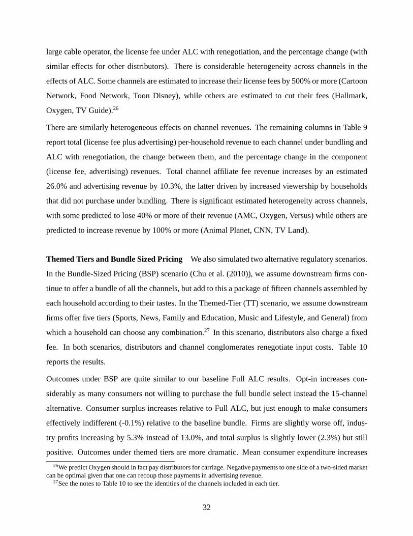
large cable operator, the license fee under ALC with renegotiation, and the percentage change (with

similar effects for other distributors). There is considerable heterogeneity across channels in the

effects of ALC. Some channels are estimated to increase their license fees by 500% or more (Cartoon

Network, Food Network, Toon Disney), while others are estimated to cut their fees (Hallmark,

Oxygen, TV Guide).26

There are similarly heterogeneous effects on channel revenues. The remaining columns in Table 9

report total (license fee plus advertising) per-householdrevenue to each channel under bundling and

ALC with renegotiation, the change between them, and the percentage change in the component

(license fee, advertising) revenues. Total channel affiliate fee revenue increases by an estimated

26.0% and advertising revenue by 10.3%, the latter driven byincreased viewership by households

that did not purchase under bundling. There is significant estimated heterogeneity across channels,

with some predicted to lose 40% or more of their revenue (AMC,Oxygen, Versus) while others are

predicted to increase revenue by 100% or more (Animal Planet, CNN, TV Land).

Themed Tiers and Bundle Sized Pricing We also simulated two alternative regulatory scenarios.

In the Bundle-Sized Pricing (BSP) scenario (Chu et al. (2010)), we assume downstream firms con-

tinue to offer a bundle of all the channels, but add to this a package of fifteen channels assembled by

each household according to their tastes. In the Themed-Tier (TT) scenario, we assume downstream

firms offer five tiers (Sports, News, Family and Education, Music and Lifestyle, and General) from

which a household can choose any combination.27 In this scenario, distributors also charge a fixed

fee. In both scenarios, distributors and channel conglomerates renegotiate input costs. Table 10

reports the results.

Outcomes under BSP are quite similar to our baseline Full ALCresults. Opt-in increases con-

siderably as many consumers not willing to purchase the fullbundle select instead the 15-channel

alternative. Consumer surplus increases relative to Full ALC, but just enough to make consumers

effectively indifferent (-0.1%) relative to the baseline bundle. Firms are slightly worse off, indus-

try profits increasing by 5.3% instead of 13.0%, and total surplus is slightly lower (2.3%) but still

positive. Outcomes under themed tiers are more dramatic. Mean consumer expenditure increases

26We predict Oxygen should in fact pay distributors for carriage. Negative payments to one side of a two-sided marketcan be optimal given that one can recoup those payments in advertising revenue.

27See the notes to Table 10 to see the identities of the channelsincluded in each tier.

32

considerably despite a fall in channels watched. Estimatedconsumer surplus therefore falls consid-

erably (-20.7%). Channel profits soar, yielding an aggregate predicted industry profit increase of

31.1%. Total surplus remains weakly positive.

Results Summary Our findings confirm the intuition regarding the likely effects of ALC described

in Section 2. When we do not allow for renegotiation (Table 8,Columns 2-3), we turn off the

input-cost-raising bargaining effect and find consumer surplus increases considerably (+16.7%) and

industry profits fall (-3.7%). As suggested by much of the bundling literature, for fixed input costs,

we find bundling transfers surplus from consumers to firms. When we allow for renegotiation (Ta-

ble 8, Columns 4-5), costs rise (+145.2%), prices follow suit, and these consumer surplus gains are

eliminated (-1.0%). Things are even worse for consumers under themed tiers (Table 10, Columns 4

& 7). The bundling of channels within the tiers eliminates much of the consumer surplus benefits

accruing under Full ALC andstill yields (67%) higher input costs. This worst-of-both-worlds out-

come significantly lowers consumer surplus (-20.7%). Our qualitative conclusion is that consumers

could in principle benefit from mandatory à la carte at existing input costs, but would not in practice

benefit due to input cost renegotiation in an à la carte world.

Robustness Our goal is to accurately measure the welfare effects of à la carte pricing in multichan-

nel television markets. As such, it is important to have confidence that this fundamental conclusion

is robust and not sensitive to particular assumptions underlying the model, estimation, or counterfac-

tual simulations. In Appendix B, we consider the robustnessof our results to alternative assumptions

on demand, cost, and bargaining, including allowing for positive channel margins for distributors in

the counterfactual, different distributional assumptions for preferences, turning off unobserved cor-

relation in tastes, and allowing renegotiated input costs to be half or double what we estimate. Of

these, only the last has a material effect on our welfare estimates and the most likely direction for

these (input cost doubling) merely reinforces our qualitative conclusions that à la carte is unlikely to

benefit consumers.

33

8 Conclusion

This paper has combined a model of the multichannel television industry with market and viewership

data in order to evaluate the welfare effects of proposed à lacarte pricing regulations. We extend

a standard demand model to a setting of joint purchasing and viewership decisions and combine it

with a model of distributor pricing and bundling, and channel-distributor bargaining. We estimate

the model using demand, pricing, viewership, and cost data from the industry. We use the estimated

model to simulate an unrealized regulatory environment: à la carte pricing regulations. Critically, we

allow for the renegotiation of supply contracts under à la carte and find that total input costs for the

49 channels in our analysis would rise by 145.2%. We compare the distributions of consumer and

producer surplus under a simulated bundling setting with those under à la carte allowing for these

cost increases and predict that, in the short run, consumer welfare would decrease approximately

1.0% under à la carte regulations, while industry profits andtotal surplus would increase by 13.0%

and 5.3%, respectively. Any implementation or marketing costs of à la carte could make it worse for

all.

One could improve our analysis of bundling in this industry in future work by either improving upon

the specifics of the model and estimation we propose, or by adding more levels of strategic behavior.

Regarding the former, we employed a model of bargaining which can be improved upon in several

dimensions. An extensive form game which accounts for the information asymmetries about secret

contracts would be a major improvement. Regarding the latter, the long-run effects of à la carte

regulations on entry, exit, content, and quality of channels are often raised as concerns by policy

makers.

34

Figure 1: Dispersion in WTP for components is higher than dispersion in WTP for a bundle

0 0.2 0.4 0.6 0.8 10

2

4

6

8

10

12

14

16

Market Share

Pric

e

Demand for Components and Demand for BundleAdams and Yellen QJE 1976

Demand for Good 1Demand for Good 2Demand for Bundle

Figure 2: Nash Bargaining for Input Costs

00.511.520

2

4

6

8

10

12

Nash Product0 0.2 0.4 0.6 0.8 1

0

2

4

6

8

10

12

Pric

e

Market Share

Πf

Πc

τ*

p*

DemandMarg. Revenue

00.511.522.50

2

4

6

8

10

12

Nash Product0 0.2 0.4 0.6 0.8 1

0

2

4

6

8

10

12

Market Share

τbun*

τalc*

Less Dispersion (Bun)More Dispersion (ALC)

Notes:These figures provide the intuition for the determination ofinput costs under Nash Bargaining. The left figure

shows the value for the input cost that maximizes the Nash Product under bilateral monopoly with linear fee contracts

and symmetric bargaining parameters. The solid lines in theright panel of the left figure show the demand and marginal

revenue for the product faced by the downstream firm. Total (gross) profit is divided between the downstream distributor

(πf ) and the upstream content providers (πc) according to an input cost (τ ). The marginal cost to the content provider

is assumed to be zero. The left panel of the left figure reportsthe value of Nash Product (as in Equation (7) for different

values ofτ . The reported input cost maximizes the Nash Product.

The right figure demonstrates the consequences to input costs of the firm facing a product with more dispersion in

tastes (as typically happens under à la carte pricing). At the optimal input price in the left figure, the downstream firm

wishes to raise price and earns a greater share of the total profit. The upstream content provider recognizes this and

bargains for a higher input cost. These dynamics are evidentin the shape of the Nash Product for the more dispersed

tastes.

35

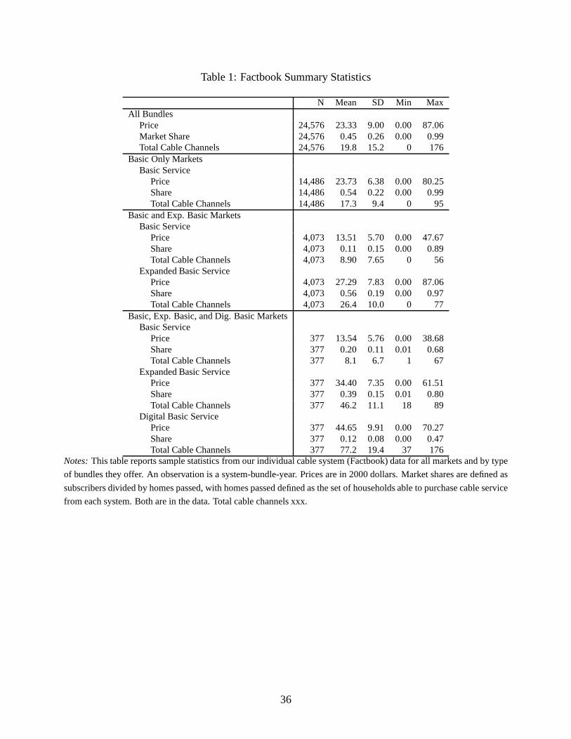
Table 1: Factbook Summary Statistics

N Mean SD Min MaxAll Bundles

Price 24,576 23.33 9.00 0.00 87.06Market Share 24,576 0.45 0.26 0.00 0.99Total Cable Channels 24,576 19.8 15.2 0 176

Basic Only MarketsBasic Service

Price 14,486 23.73 6.38 0.00 80.25Share 14,486 0.54 0.22 0.00 0.99Total Cable Channels 14,486 17.3 9.4 0 95

Basic and Exp. Basic MarketsBasic Service

Price 4,073 13.51 5.70 0.00 47.67Share 4,073 0.11 0.15 0.00 0.89Total Cable Channels 4,073 8.90 7.65 0 56

Expanded Basic ServicePrice 4,073 27.29 7.83 0.00 87.06Share 4,073 0.56 0.19 0.00 0.97Total Cable Channels 4,073 26.4 10.0 0 77

Basic, Exp. Basic, and Dig. Basic MarketsBasic Service

Price 377 13.54 5.76 0.00 38.68Share 377 0.20 0.11 0.01 0.68Total Cable Channels 377 8.1 6.7 1 67

Expanded Basic ServicePrice 377 34.40 7.35 0.00 61.51Share 377 0.39 0.15 0.01 0.80Total Cable Channels 377 46.2 11.1 18 89

Digital Basic ServicePrice 377 44.65 9.91 0.00 70.27Share 377 0.12 0.08 0.00 0.47Total Cable Channels 377 77.2 19.4 37 176

Notes:This table reports sample statistics from our individual cable system (Factbook) data for all markets and by type

of bundles they offer. An observation is a system-bundle-year. Prices are in 2000 dollars. Market shares are defined as

subscribers divided by homes passed, with homes passed defined as the set of households able to purchase cable service

from each system. Both are in the data. Total cable channels xxx.

36

Table 2: Channel Summary Statistics

Cable System Carriage Household ViewershipData Source Factbook Nielsen Mediamark

Any Tier Basic Tier Mean Mean StdDevChannel (Pcntge) (Pcntge) Rating Rating Rating CumeABC Family Channel 89.9 76.1 0.4 0.6 1.5 31.6AMC 47.1 30.7 0.5 0.6 1.4 27.2Animal Planet 17.9 11.9 0.3 0.6 1.5 34.8Arts & Entertainment 63.3 48.7 0.7 0.8 1.7 37.8BET Networks 16.3 11.0 0.4 0.3 1.5 10.6Bravo 7.7 3.3 0.2 0.2 0.7 14.4Cartoon Network 23.4 15.6 1.6 0.5 1.8 20.9CNBC 29.5 19.8 0.2 0.5 1.4 29.5CNN 93.5 78.0 0.7 1.8 3.0 53.8Comedy Central 18.3 11.0 0.5 0.5 1.3 27.6Country Music TV 46.1 37.3 0.2 0.2 1.0 13.5Court TV 10.7 4.5 0.4 0.4 1.4 18.1Discovery Channel 85.6 71.9 0.6 1.1 1.9 50.9Disney Channel 37.8 29.3 1.2 0.5 1.4 21.2E! Entertainment Television 17.1 10.8 0.3 0.3 0.9 24.4ESPN 96.0 77.0 0.9 1.1 2.2 40.7ESPN 2 30.8 21.2 0.3 0.5 1.4 25.2Food Network 8.3 4.4 0.4 0.5 1.5 26.7Fox News Channel 14.9 9.8 0.8 1.0 2.2 40.0Fox Sports Net 27.7 18.3 0.3 0.4 1.2 20.2FX 15.1 9.6 0.5 0.4 1.2 23.3GSN 4.0 0.7 0.2 0.2 0.9 7.4Golf Channel 5.6 1.8 0.0 0.1 0.6 6.9Hallmark Channel 4.7 3.1 0.3 0.2 1.0 10.8HGTV 20.2 13.0 0.6 0.6 1.6 27.5History Channel 26.3 18.2 0.6 0.8 1.7 37.9Lifetime 55.5 41.8 0.9 1.0 2.2 34.4MSNBC 9.3 5.0 0.3 0.5 1.3 30.2MTV 43.3 30.2 0.7 0.4 1.4 21.8MTV2 0.7 0.1 0.0 0.1 0.7 7.8National Geographic Channel 3.3 1.1 0.1 0.2 0.8 13.2Nickelodeon 67.9 52.8 1.8 0.4 1.3 17.7Oxygen 1.1 0.3 0.1 0.1 0.5 7.2Syfy 27.2 18.4 0.5 0.4 1.4 20.9SoapNet 1.8 0.4 0.1 0.1 0.6 2.5Speed Channel 7.0 3.1 0.1 0.1 0.7 7.8Spike TV 18.8 14.3 0.5 0.4 1.1 18.9TBS Superstation 96.3 91.2 1.1 0.9 1.7 39.8The Weather Channel 57.2 46.0 0.3 0.7 1.3 50.3TLC 39.6 29.8 0.5 0.5 1.3 29.0TNT 82.2 63.8 1.3 0.9 1.8 41.3Toon Disney 4.8 2.0 0.2 0.1 0.7 6.1Travel Channel 12.4 8.2 0.2 0.2 0.7 18.7TV Guide Channel 13.4 11.2 0.2 0.2 0.6 17.5TV Land 19.5 14.9 0.8 0.6 1.8 23.9USA Network 86.1 66.7 1.2 0.8 1.6 37.4Versus 4.7 1.4 0.1 0.1 0.5 4.8VH1 32.6 22.6 0.4 0.3 0.9 18.2WE: Women’s Entertainment 3.2 0.8 0.1 0.1 0.5 5.9

Notes: This table reports summary statistics for channels from both our cable system (Factbook) and viewership

(Nielsen, Mediamark) data. The channels reported are thosecable channels for which we could get complete data

from all three channel data sources used in our analysis. Thefirst column reports the average carriage of each cable

channel on any offered tier of service across our system-years. The second column reports average channel carriage on

just the Basic tier. The last four columns report summary statistics about household viewing patterns across channels

from our Nielsen and Mediamark data. The third column reports the average rating for all programs on that channel for

the four Nielsen sweeps months (Feb, May, Aug, Nov) between 2000 and 2006. The fourth and fifth columns report

the mean and standard deviation of the fraction of households reporting viewing each channel per hour for our sample

of Mediamark households from 2000 to 2007. This is analogousto an average Nielsen rating for that channel and we

therefore call them “ratings” above. The last column reports the fraction of Mediamark households reporting positive

viewing for each channel. This is known as the channel’s “cume,” short for cumulative audience.37

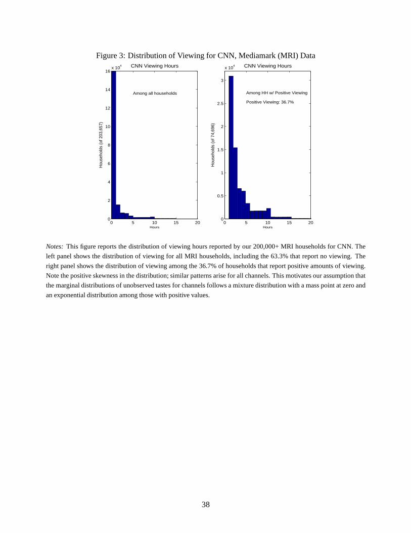
Figure 3: Distribution of Viewing for CNN, Mediamark (MRI) Data

0 5 10 15 200

2

4

6

8

10

12

14

16x 10

4 CNN Viewing Hours

Hou

seho

lds

(of 2

03,6

57)

Hours

Among all households

0 5 10 15 200

0.5

1

1.5

2

2.5

3

x 104 CNN Viewing Hours

Hou

seho

lds

(of 7

4,69

6)

Hours

Among HH w/ Positive Viewing

Positive Viewing: 36.7%

Notes:This figure reports the distribution of viewing hours reported by our 200,000+ MRI households for CNN. The

left panel shows the distribution of viewing for all MRI households, including the 63.3% that report no viewing. The

right panel shows the distribution of viewing among the 36.7% of households that report positive amounts of viewing.

Note the positive skewness in the distribution; similar patterns arise for all channels. This motivates our assumptionthat

the marginal distributions of unobserved tastes for channels follows a mixture distribution with a mass point at zero and

an exponential distribution among those with positive values.

38

Figure 4: Estimated WTP for a Subset of Channels

0 2 4 6 80

1000

2000

3000ABC Family Channel

Hou

seho

lds

(of 2

0,00

0)

WTP (Year 2000 Dollars)

Pos: 49%

0 5 100

1000

2000

3000BET Networks

Hou

seho

lds

(of 2

0,00

0)WTP (Year 2000 Dollars)

Pos: 39%

0 10 200

1000

2000

3000

4000CNN

Hou

seho

lds

(of 2

0,00

0)

WTP (Year 2000 Dollars)

Pos: 69%

0 5 100

2000

4000

6000Comedy Central

Hou

seho

lds

(of 2

0,00

0)

WTP (Year 2000 Dollars)

Pos: 58%

0 5 100

2000

4000

6000Disney Channel

Hou

seho

lds

(of 2

0,00

0)

WTP (Year 2000 Dollars)

Pos: 61%

0 5 10 150

1000

2000

3000ESPN

Hou

seho

lds

(of 2

0,00

0)

WTP (Year 2000 Dollars)

Pos: 57%

0 5 100

2000

4000

6000MTV

Hou

seho

lds

(of 2

0,00

0)

WTP (Year 2000 Dollars)

Pos: 61%

0 5 100

2000

4000

6000TNT

Hou

seho

lds

(of 2

0,00

0)

WTP (Year 2000 Dollars)

Pos: 72%

0 5 100

1000

2000

3000

4000USA Network

Hou

seho

lds

(of 2

0,00

0)

WTP (Year 2000 Dollars)

Pos: 47%

Notes:This figure documents the estimated willingness-to-pay fora subset of cable channels among 20,000 simulated

households. Reported is the share of those households that value each network positively and the distribution of WTP

among that subset. In each figure, the y-axis reports households and the x-axis reports WTP in 2000 dollars.

39

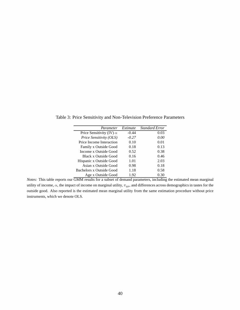
Table 3: Price Sensitivity and Non-Television Preference Parameters

Parameter Estimate Standard ErrorPrice Sensitivity (IV)α -0.44 0.03Price Sensitivity (OLS) -0.27 0.00

Price Income Interaction 0.10 0.01Family x Outside Good 0.18 0.13Income x Outside Good 0.52 0.38

Black x Outside Good 0.16 0.46Hispanic x Outside Good 1.01 2.03

Asian x Outside Good 0.98 0.18Bachelors x Outside Good 1.18 0.58

Age x Outside Good 1.92 0.30Notes:This table reports our GMM results for a subset of demand parameters, including the estimated mean marginal

utility of income,α, the impact of income on marginal utility,πyp, and differences across demographics in tastes for the

outside good. Also reported is the estimated mean marginal utility from the same estimation procedure without price

instruments, which we denote OLS.

40

Table 4: Estimated WTP

Mean Mean HighestMean StdDev Share WTP WTP Correlated

Channel WTP WTP Positive Family HH Black HH ChannelABC Family Channel 1.39 2.13 0.49 1.44 1.48 TV LandAMC 1.25 1.44 0.51 1.06 1.54 MSNBCAnimal Planet 1.96 3.06 0.54 1.97 1.78 National Geographic ChannelArts & Entertainment 1.84 2.28 0.58 1.67 1.82 VH1BET Networks 1.14 2.26 0.39 1.11 4.13 MTV2Bravo 0.59 0.68 0.58 0.58 0.67 ESPNCartoon Network 1.89 3.76 0.48 2.07 2.27 Disney ChannelCNBC 1.92 2.77 0.54 1.74 1.88 CNNCNN 4.82 5.44 0.69 4.51 7.37 CNBCComedy Central 1.38 2.35 0.58 1.38 1.32 VH1Country Music TV 0.78 1.35 0.56 0.78 0.67 Food NetworkCourt TV 1.65 2.88 0.51 1.70 2.10 Animal PlanetDiscovery Channel 2.53 2.89 0.63 2.36 2.59 Animal PlanetDisney Channel 1.35 2.27 0.61 1.45 1.63 NickelodeonE! Entertainment Television 1.00 1.56 0.62 1.00 0.91 WE: Womens EntertainmentESPN 2.75 4.08 0.57 2.55 3.33 ESPN 2ESPN 2 1.70 2.92 0.55 1.64 1.83 ESPNFood Network 1.86 2.95 0.69 1.87 2.15 TV Guide ChannelFox News Channel 3.74 5.85 0.58 3.89 4.20 CNNFox Sports Net 1.58 2.78 0.56 1.54 1.37 ESPN 2FX 1.30 2.41 0.48 1.33 1.35 USA NetworkGSN 0.73 3.34 0.07 0.78 1.37 ESPN 2Golf Channel 0.68 2.62 0.09 0.56 0.84 HGTVHallmark Channel 1.26 4.00 0.13 1.21 1.84 VersusHGTV 2.55 4.75 0.41 2.58 3.14 Food NetworkHistory Channel 2.48 3.96 0.37 2.40 2.67 Arts & EntertainmentLifetime 2.11 3.84 0.27 2.28 5.14 AMCMSNBC 1.75 3.58 0.25 1.60 2.71 AMCMTV 1.30 2.20 0.61 1.29 1.37 VH1MTV2 0.65 1.32 0.46 0.66 0.64 VH1National Geographic Channel 0.94 1.48 0.63 0.94 0.85 Animal PlanetNickelodeon 1.20 2.53 0.45 1.29 1.30 Disney ChannelOxygen 0.33 0.37 0.59 0.42 0.49 Speed ChannelSyfy 1.66 2.94 0.53 1.66 1.68 USA NetworkSoapNet 0.39 0.84 0.40 0.41 0.51 TBS SuperstationSpeed Channel 0.24 0.30 0.56 0.29 0.17 VersusSpike TV 1.16 1.97 0.54 1.15 1.05 The Weather ChannelTBS Superstation 1.94 2.72 0.67 1.89 2.05 TNTThe Weather Channel 1.53 1.66 0.65 1.44 1.59 Spike TVTLC 1.76 2.72 0.58 1.80 1.55 Discovery ChannelTNT 2.19 2.92 0.72 2.17 2.15 TBS SuperstationToon Disney 0.37 1.50 0.12 0.48 0.89 LifetimeTravel Channel 0.75 2.52 0.11 0.77 0.85 NickelodeonTV Guide Channel 0.47 0.74 0.56 0.50 0.63 Food NetworkTV Land 2.08 3.56 0.53 2.12 2.46 ABC Family ChannelUSA Network 1.89 2.71 0.47 2.03 2.54 TNTVersus 0.20 0.28 0.50 0.24 0.20 Speed ChannelVH1 0.74 1.27 0.55 0.75 0.84 MTV2WE: Womens Entertainment 0.37 0.59 0.49 0.40 0.38 National Geographic Channel

Notes:This table reports information of the distribution of WTP for channels implied by our estimates. The first two

columns report the mean and standard deviation in WTP for each channel among those that value it positively. The third

column reports the estimate share of households that do so. The fourth and fifth columns report estimated WTP among

family and black households. The last column reports the channel estimated to have the highest correlation in WTP for

each channel. WTP is measured in year 2000 dollars per month per household.

41

Table 5: Input Cost Parameters

All No BundlingMoments Moments

Standard StandardParameter Estimate Error Estimate ErrorConstant -0.03 0.00 0.00 0.00Kagan Scale 1.04 0.01 1.07 0.01MSO Size -0.04 0.01 -0.05 0.01Vertical Integration 0.00 0.07 0.07 0.08

Notes:This table reports the impact of various factors on our estimated input costs. Kagan scale refers to the input cost

for that channel as estimated by Kagan World Media (2008). Distributor (MSO) size is measured in tens of millions of

households. Vertical integration is the share of the channel owned by that distributor (between 0 and 1).

Table 6: Regression Analysis of Distributor Size on Price and Estimated Marginal CostPrice Regression Estimated Marginal Cost Regression

Coef SE t Statistic Coef SE t StatisticDistributor Size -0.057 0.010 -5.720-0.100 0.038 -2.632

Number of Integrated Channels -0.005 0.058 -0.086-0.251 0.216 -1.160Dummy Variables

Channels Yes YesYear Yes YesTier Yes Yes

Number of Bundles Yes YesYear x Tier Yes Yes

Number of Bundles x Tier Yes YesN 24576 24576

R-squared 0.547 0.211F(262, 24313) 111.92 24.82

Notes:This table reports the results of regressions designed to highlight the identification of our input cost estimates.

The first set of columns reports the results of a regression ofbundle prices on the size of the distributor offering the

bundle and a sum of the number of vertically integrated channels in the distributor’s bundle. We condition on various

variables that might affect marginal costs. The second set of columns reports the results of a regression of our estimated

bundle marginal costs on the same covariates.

42

Table 7: Conglomerate Bargaining Parameters

Conglomerate Big Cable Small Cable DirecTV Dish NetworkABC Disney 0.352 0.359 0.306 0.319

Viacom 0.582 0.588 0.678 0.696NBC Universal 0.518 0.528 0.581 0.594

Comcast Content Division 0.559 0.575 0.623 0.638Scripps 0.550 0.568 0.613 0.625

News Corporation 0.450 0.450 0.456 0.469Rainbow Media 0.756 0.759 0.784 0.791

Discovery Networks 0.522 0.535 0.586 0.604Time Warner 0.421 0.431 0.450 0.463

Hallmark 0.736 0.752 0.793 0.803Lifetime 0.450 0.459 0.497 0.509Oxygen 0.761 0.770 0.786 0.794

Weather Channel 0.556 0.569 0.619 0.628TV Guide 0.785 0.795 0.832 0.836

Notes:This table reports our estimated bargaining parameters forchannel conglomerates versus distributors of various

types. Smaller values of the bargaining parameters indicate relatively more bargaining power for channels. Channel

conglomerates are ABC Disney (ABC Family Channel, Disney Channel, ESPN, ESPN2, Soap Net, Toon Disney), Vi-

acom (BET Networks, Comedy Central, Country Music TV, GSN, MTV, MTV2, Nickelodeon, Spike TV, TV Land,

VH1), NBC Universal (Arts & Entertainment, Bravo, CNBC, MSNBC, Syfy, USA Network), Comcast (E! Entertain-

ment Television, Golf Channel, Versus), Scripps (Food Network, HGTV), News Corporation (Fox News Channel, Fox

Sports Net, FX, National Geographic Channel, Speed Channel), Rainbow Media (AMC, WE: Women’s Entertainment),

Discovery Networks (Animal Planet, Discovery Channel, History Channel, TLC, Travel Channel), Time Warner (Car-

toon Network, CNN, Court TV, TBS Superstation, TNT). Hallmark, Lifetime, Oxygen, Weather Channel, and TV Guide

are single-channel “conglomerates.” See the end of Section5 for descriptions of the distributor types.

43

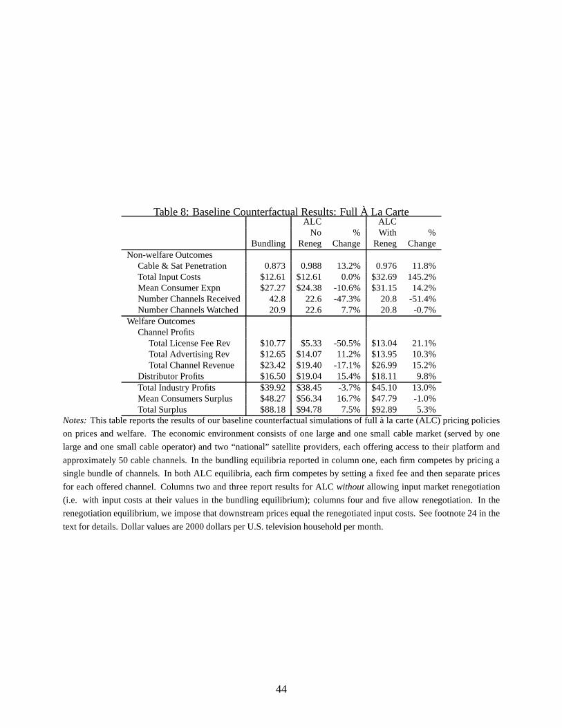
Table 8: Baseline Counterfactual Results: Full À La CarteALC ALC

No % With %Bundling Reneg Change Reneg Change

Non-welfare OutcomesCable & Sat Penetration 0.873 0.988 13.2% 0.976 11.8%Total Input Costs $12.61 $12.61 0.0% $32.69 145.2%Mean Consumer Expn $27.27 $24.38 -10.6% $31.15 14.2%Number Channels Received 42.8 22.6 -47.3% 20.8 -51.4%Number Channels Watched 20.9 22.6 7.7% 20.8 -0.7%

Welfare OutcomesChannel Profits

Total License Fee Rev $10.77 $5.33 -50.5% $13.04 21.1%Total Advertising Rev $12.65 $14.07 11.2% $13.95 10.3%Total Channel Revenue $23.42 $19.40 -17.1% $26.99 15.2%

Distributor Profits $16.50 $19.04 15.4% $18.11 9.8%Total Industry Profits $39.92 $38.45 -3.7% $45.10 13.0%Mean Consumers Surplus $48.27 $56.34 16.7% $47.79 -1.0%Total Surplus $88.18 $94.78 7.5% $92.89 5.3%

Notes:This table reports the results of our baseline counterfactual simulations of full à la carte (ALC) pricing policies

on prices and welfare. The economic environment consists ofone large and one small cable market (served by one

large and one small cable operator) and two “national” satellite providers, each offering access to their platform and

approximately 50 cable channels. In the bundling equilibria reported in column one, each firm competes by pricing a

single bundle of channels. In both ALC equilibria, each firm competes by setting a fixed fee and then separate prices

for each offered channel. Columns two and three report results for ALC without allowing input market renegotiation

(i.e. with input costs at their values in the bundling equilibrium); columns four and five allow renegotiation. In the

renegotiation equilibrium, we impose that downstream prices equal the renegotiated input costs. See footnote 24 in the

text for details. Dollar values are 2000 dollars per U.S. television household per month.

44

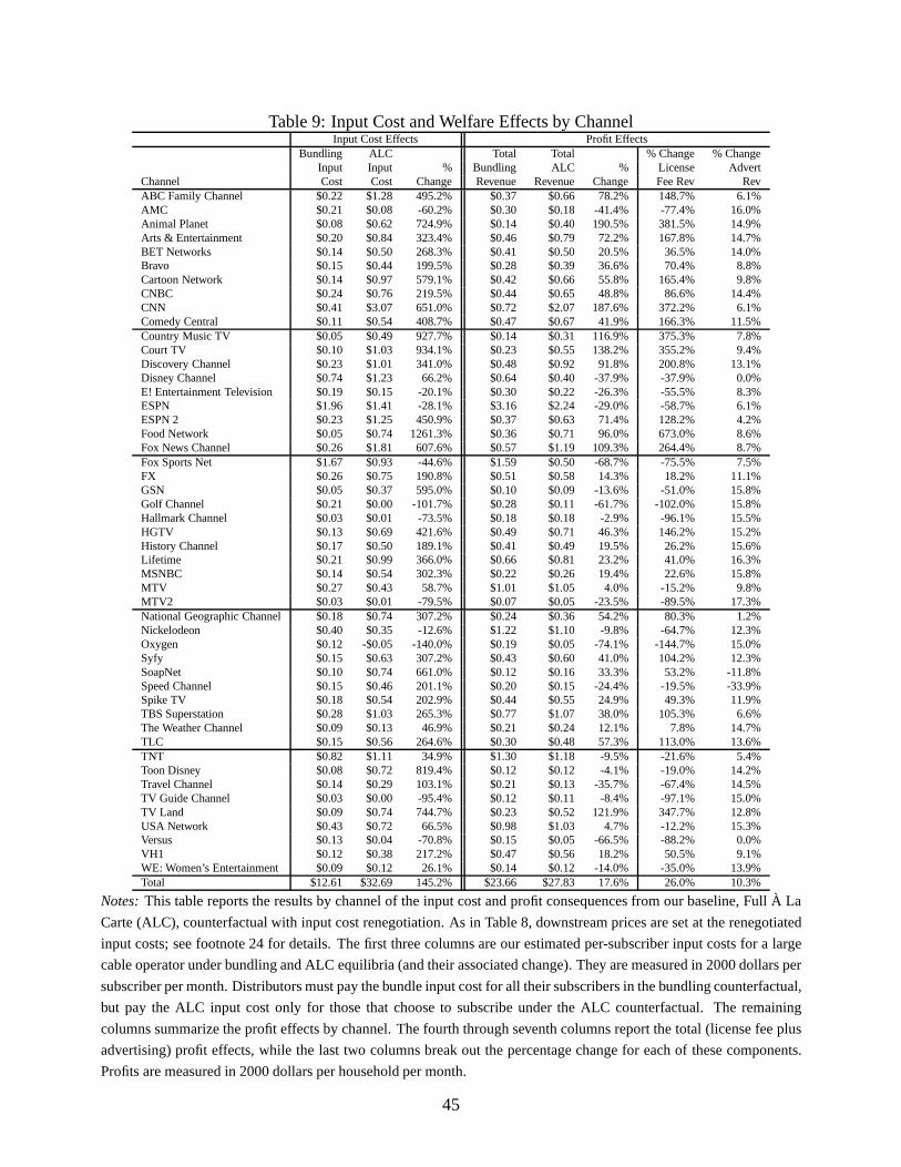
Table 9: Input Cost and Welfare Effects by ChannelInput Cost Effects Profit Effects

Bundling ALC Total Total % Change % ChangeInput Input % Bundling ALC % License Advert

Channel Cost Cost Change Revenue Revenue Change Fee Rev RevABC Family Channel $0.22 $1.28 495.2% $0.37 $0.66 78.2% 148.7% 6.1%AMC $0.21 $0.08 -60.2% $0.30 $0.18 -41.4% -77.4% 16.0%Animal Planet $0.08 $0.62 724.9% $0.14 $0.40 190.5% 381.5% 14.9%Arts & Entertainment $0.20 $0.84 323.4% $0.46 $0.79 72.2% 167.8% 14.7%BET Networks $0.14 $0.50 268.3% $0.41 $0.50 20.5% 36.5% 14.0%Bravo $0.15 $0.44 199.5% $0.28 $0.39 36.6% 70.4% 8.8%Cartoon Network $0.14 $0.97 579.1% $0.42 $0.66 55.8% 165.4% 9.8%CNBC $0.24 $0.76 219.5% $0.44 $0.65 48.8% 86.6% 14.4%CNN $0.41 $3.07 651.0% $0.72 $2.07 187.6% 372.2% 6.1%Comedy Central $0.11 $0.54 408.7% $0.47 $0.67 41.9% 166.3% 11.5%Country Music TV $0.05 $0.49 927.7% $0.14 $0.31 116.9% 375.3% 7.8%Court TV $0.10 $1.03 934.1% $0.23 $0.55 138.2% 355.2% 9.4%Discovery Channel $0.23 $1.01 341.0% $0.48 $0.92 91.8% 200.8% 13.1%Disney Channel $0.74 $1.23 66.2% $0.64 $0.40 -37.9% -37.9% 0.0%E! Entertainment Television $0.19 $0.15 -20.1% $0.30 $0.22 -26.3% -55.5% 8.3%ESPN $1.96 $1.41 -28.1% $3.16 $2.24 -29.0% -58.7% 6.1%ESPN 2 $0.23 $1.25 450.9% $0.37 $0.63 71.4% 128.2% 4.2%Food Network $0.05 $0.74 1261.3% $0.36 $0.71 96.0% 673.0% 8.6%Fox News Channel $0.26 $1.81 607.6% $0.57 $1.19 109.3% 264.4% 8.7%Fox Sports Net $1.67 $0.93 -44.6% $1.59 $0.50 -68.7% -75.5% 7.5%FX $0.26 $0.75 190.8% $0.51 $0.58 14.3% 18.2% 11.1%GSN $0.05 $0.37 595.0% $0.10 $0.09 -13.6% -51.0% 15.8%Golf Channel $0.21 $0.00 -101.7% $0.28 $0.11 -61.7% -102.0% 15.8%Hallmark Channel $0.03 $0.01 -73.5% $0.18 $0.18 -2.9% -96.1% 15.5%HGTV $0.13 $0.69 421.6% $0.49 $0.71 46.3% 146.2% 15.2%History Channel $0.17 $0.50 189.1% $0.41 $0.49 19.5% 26.2% 15.6%Lifetime $0.21 $0.99 366.0% $0.66 $0.81 23.2% 41.0% 16.3%MSNBC $0.14 $0.54 302.3% $0.22 $0.26 19.4% 22.6% 15.8%MTV $0.27 $0.43 58.7% $1.01 $1.05 4.0% -15.2% 9.8%MTV2 $0.03 $0.01 -79.5% $0.07 $0.05 -23.5% -89.5% 17.3%National Geographic Channel $0.18 $0.74 307.2% $0.24 $0.36 54.2% 80.3% 1.2%Nickelodeon $0.40 $0.35 -12.6% $1.22 $1.10 -9.8% -64.7% 12.3%Oxygen $0.12 -$0.05 -140.0% $0.19 $0.05 -74.1% -144.7% 15.0%Syfy $0.15 $0.63 307.2% $0.43 $0.60 41.0% 104.2% 12.3%SoapNet $0.10 $0.74 661.0% $0.12 $0.16 33.3% 53.2% -11.8%Speed Channel $0.15 $0.46 201.1% $0.20 $0.15 -24.4% -19.5% -33.9%Spike TV $0.18 $0.54 202.9% $0.44 $0.55 24.9% 49.3% 11.9%TBS Superstation $0.28 $1.03 265.3% $0.77 $1.07 38.0% 105.3% 6.6%The Weather Channel $0.09 $0.13 46.9% $0.21 $0.24 12.1% 7.8% 14.7%TLC $0.15 $0.56 264.6% $0.30 $0.48 57.3% 113.0% 13.6%TNT $0.82 $1.11 34.9% $1.30 $1.18 -9.5% -21.6% 5.4%Toon Disney $0.08 $0.72 819.4% $0.12 $0.12 -4.1% -19.0% 14.2%Travel Channel $0.14 $0.29 103.1% $0.21 $0.13 -35.7% -67.4% 14.5%TV Guide Channel $0.03 $0.00 -95.4% $0.12 $0.11 -8.4% -97.1% 15.0%TV Land $0.09 $0.74 744.7% $0.23 $0.52 121.9% 347.7% 12.8%USA Network $0.43 $0.72 66.5% $0.98 $1.03 4.7% -12.2% 15.3%Versus $0.13 $0.04 -70.8% $0.15 $0.05 -66.5% -88.2% 0.0%VH1 $0.12 $0.38 217.2% $0.47 $0.56 18.2% 50.5% 9.1%WE: Women’s Entertainment $0.09 $0.12 26.1% $0.14 $0.12 -14.0% -35.0% 13.9%Total $12.61 $32.69 145.2% $23.66 $27.83 17.6% 26.0% 10.3%

Notes:This table reports the results by channel of the input cost and profit consequences from our baseline, Full À La

Carte (ALC), counterfactual with input cost renegotiation. As in Table 8, downstream prices are set at the renegotiated

input costs; see footnote 24 for details. The first three columns are our estimated per-subscriber input costs for a large

cable operator under bundling and ALC equilibria (and theirassociated change). They are measured in 2000 dollars per

subscriber per month. Distributors must pay the bundle input cost for all their subscribers in the bundling counterfactual,

but pay the ALC input cost only for those that choose to subscribe under the ALC counterfactual. The remaining

columns summarize the profit effects by channel. The fourth through seventh columns report the total (license fee plus

advertising) profit effects, while the last two columns break out the percentage change for each of these components.

Profits are measured in 2000 dollars per household per month.

45

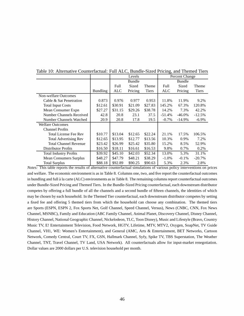
Table 10: Alternative Counterfactual: Full ALC, Bundle-Sized Pricing, and Themed TiersLevels Percent ChangeBundle Bundle

Full Sized Theme Full Sized ThemeBundling ALC Pricing Tiers ALC Pricing Tiers

Non-welfare OutcomesCable & Sat Penetration 0.873 0.976 0.977 0.953 11.8% 11.9% 9.2%Total Input Costs $12.61 $30.91 $21.09 $27.83 145.2% 67.3% 120.8%Mean Consumer Expn $27.27 $31.15 $29.26 $38.78 14.2% 7.3% 42.2%Number Channels Received 42.8 20.8 23.1 37.5 -51.4% -46.0% -12.5%Number Channels Watched 20.9 20.8 17.8 19.5 -0.7% -14.9% -6.9%

Welfare OutcomesChannel Profits

Total License Fee Rev $10.77 $13.04 $12.65 $22.24 21.1% 17.5% 106.5%Total Advertising Rev $12.65 $13.95 $12.77 $13.56 10.3% 0.9% 7.2%Total Channel Revenue $23.42 $26.99 $25.42 $35.80 15.2% 8.5% 52.9%

Distributor Profits $16.50 $18.11 $16.61 $16.53 9.8% 0.7% 0.2%Total Industry Profits $39.92 $45.10 $42.03 $52.34 13.0% 5.3% 31.1%Mean Consumers Surplus $48.27 $47.79 $48.21 $38.29 -1.0% -0.1% -20.7%Total Surplus $88.18 $92.89 $90.25 $90.63 5.3% 2.3% 2.8%

Notes:This table reports the results of alternative counterfactual simulations of various policy interventions on prices

and welfare. The economic environment is as in Table 8. Columns one, two, and five report the counterfactual outcomes

in bundling and full à la carte (ALC) environments as in Table8. The remaining columns report counterfactual outcomes

under Bundle-Sized Pricing and Themed Tiers. In the Bundle-Sized Pricing counterfactual, each downstream distributor

competes by offering a full bundle of all the channels and a second bundle of fifteen channels, the identities of which

may be chosen by each household. In the Themed Tier counterfactual, each downstream distributor competes by setting

a fixed fee and offering 5 themed tiers from which the household can choose any combination. The themed tiers

are Sports (ESPN, ESPN 2, Fox Sports Net, Golf Channel, SpeedChannel, Versus), News (CNBC, CNN, Fox News

Channel, MSNBC), Family and Education (ABC Family Channel,Animal Planet, Discovery Channel, Disney Channel,

History Channel, National Geographic Channel, Nickelodeon, TLC, Toon Disney), Music and Lifestyle (Bravo, Country

Music TV, E! Entertainment Television, Food Network, HGTV,Lifetime, MTV, MTV2, Oxygen, SoapNet, TV Guide

Channel, VH1, WE: Women’s Entertainment), and General (AMC, Arts & Entertainment, BET Networks, Cartoon

Network, Comedy Central, Court TV, FX, GSN, Hallmark Channel, Syfy, Spike TV, TBS Superstation, The Weather

Channel, TNT, Travel Channel, TV Land, USA Network). All counterfactuals allow for input-market renegotiation.

Dollar values are 2000 dollars per U.S. television household per month.

46

References

Adams, William James and Janet L. Yellen, “Commodity Bundling and the Burden of Monopoly,”

The Quarterly Journal of Economics, 1976,90 (3), 475–498.

Armstrong, M. and J. Vickers, “Competitive Price Discrimination,”RAND Journgal of Economics,

2001,32 (4), 579–605.

Beard, T. R., G. S. Ford, R. C. Hill, and R. P. Saba, “Fragmented Duopoly: A Conceptual and

Empirical Investigation,”Journal of Business, 2005,78.

Berry, Steven, James Levinsohn, and Ariel Pakes, “Automobile Prices in Market Equilibrium,”

Econometrica, 1995,63 (4), 841–890.

, , and , “Differentiated Products Demand Systems from a Combination of Micro

and Macro Data: The New Car Market,”The Journal of Political Economy, 2004,112 (1),

68–105.

Byzalov, Dmitri , “Unbundling Cable Television: An Empirical Analysis,” 2008. mimeo, Harvard

University.

Chipty, Tasneem, “Vertical Integration, Market Foreclosure, and ConsumerWelfare in the Cable

Television Industry,”American Economic Review, 2001,91 (3), 428–453.

and Christopher Snyder, “The Role of Firm Size in Bilateral Bargaining: A Study of the

Cable Television Industry,”Review of Economics and Statistics, 1999,31 (2), 326–340.

Chu, Sean, Phillip Leslie, and Alan Sorensen, “Bundle-Size Pricing as an Approximation to

Mixed Bundling,” 2010. Forthcoming, American Economic Review.

Crawford, G. , “The Impact of the 1992 Cable Act on Household Demand and Welfare,” RAND

Journal of Economics, Autumn 2000,31 (3), 422–449.

, “The Discriminatory Incentives to Bundle in the Cable Television Industry,” 2007. forthcom-

ing, Quantitative Marketing and Economics.

47

Cremer, Jacques and Michael H. Riordan, “On Governing Multilateral Transactions with Bilat-

eral Contracts,”The RAND Journal of Economics, 1987,18 (3), 436–451.

de Fontenay, Catherine and Joshua Gans, “Bilateral Bargaining with Externalities,” 2007. Avail-

able http://works.bepress.com/joshuagans/14.

FCC, “2001 Report on Cable Industry Prices,” Technical Report,Federal Communications Com-

mission 2002. Available at http://www.fcc.gov/mb/csrptpg.html.

, “Report on the Packaging and Sale of Video Programming to the Public,” Technical

Report, Federal Communications Commission 2004. November18, 2004. Available at

http://www.fcc.gov/mb/csrptpg.html.

, “Further Report on the Packaging and Sale of Video Programming to the Public,” Tech-

nical Report, Federal Communications Commission 2006. February, 2006. Available at

http://www.fcc.gov/mb/csrptpg.html.

, “2006-2008 Report on Cable Industry Prices,” Technical Report, Federal Communications

Commission 2008. Draft internal FCC report.

GAO, “Issues Related to Competition and Subscriber Rates in theCable Television Industry,” Tech-

nical Report, General Accounting Office October 2003. GAO-04-8.

Goolsbee, Austan and Amil Petrin, “Consumer Gains from Direct Broadcast Satellites and the

Competition with Cable TV,”Econometrica, 2004,72 (2), 351–81.

Hart, Oliver and Jean Tirole , “Vertical Integration and Market Foreclosure,”Brookings Papers on

Economic Activity. Microeconomics, 1990,1990, 205–286.

Hausman, J., “Valuation of New Goods under Perfect and Imperfect Competition,” in T. Bresnahan

and R. Gordon, eds.,The Economics of New Goods, University of Chicago Press, 1996.

Ho, Katherine, “Insurer-Provider Networks in the Medical Care Market,”American Economic Re-

view, 2009,99 (1), 393–430.

Horn, Henrik and Asher Wolinsky , “Bilateral Monopoly and Incentives for Merger,”The RAND

Journal of Economics, 1988,19, 408–419.

48

Kagan World Media , “Economics of Basic Cable Television Networks,” Technical Report, Kagan

World Media 2008.

Lee, Robin S., “Dynamic Demand Estimation in Platform and Two-Sided Markets,” 2010. Working

Paper, NYU Stern.

McAfee, R. P., J. McMillan, and M. Whinston, “Multiproduct Monopoly, Commodity Bundling,

and Correlation of Values,”Quarterly Journal of Economics, 1989,104(2), 371–383.

McAfee, R. Preston and Marius Schwartz, “Opportunism in Multilateral Vertical Contracting:

Nondiscrimination, Exclusivity, and Uniformity,”The American Economic Review, 1994,84

(1), 210–230.

Muthoo, Abhinay, Bargaining Theory with Applications, Cambridge: Cambridge University Press,

1999.

Nash, John F., “The Bargaining Problem,”Econometrica, 1950,18 (2), 155–162.

Pakes, Ariel, Jack Porter, Katherine Ho, and Joy Ishii, “Moment Inequalities and Their Appli-

cation,” 2006. mimeo, Harvard University.

Petrin, Amil , “Quantifying the Benefits of New Products: The Case of the Minivan,” Journal of

Political Economy, 2003,110(4), 705–729.

Raskovich, Alexander, “Pivotal Buyers and Bargaining Position,”Journal of Industrial Economics,

2003,51 (4), 405–426.

Rennhoff, Adam D. and Konstantinos Serfes, “Estimating the Effects of a la Carte Pricing: The

Case of Cable Television,”SSRN eLibrary, 2008.

and , “The Role of Upstream-Downstream Competition on BundlingDecisions: Should

Regulators Force Firms to Unbundle?,”Journal of Economics and Management Strategy, 2009,

18, 547–588.

Reuters, “U.S. Lawmaker Urges A La Carte Cable Channel Rates,”Reuters News Service, 2003.

March 14, 2003.

49

Rochet, J.-C. and L. Stole, “Nonlinear Pricing with Random Participation,”Review of Economic

Studies, 2002,69 (1), 277–311.

Rubinstein, Ariel , “Perfect Equilibrium in a Bargaining Model,”Econometrica, 1982,50 (1), 97–

109.

Segal, Ilya and Michael D. Whinston, “Robust Predictions for Bilateral Contracting with Exter-

nalities,”Econometrica, 2003,71 (3), 757–791.

Shatz, Amy, “À la Carte Pricing May Cut Bills For Cable Customers, FCC Says,” Wall Street

Journal, 2006. February 10, 2006.

Stigler, G., “United States v. Loew’s Inc.: A Note on Block Booking,” in P. Kurland, ed.,The

Supreme Court Review: 1963, University of Chicago Press, 1963, pp. 152–157.

50

A The Multi-Channel Television Industry

The multi-channel television market is a two-sided market.Cable and satellite systems provide a

platform connecting households with both program producers and advertisers. Figure 5 provides a

graphical representation of the supply chain by which programming is produced and sold to house-

holds and audiences are created and sold to advertisers. Downward arrows represent the flow of

programming from content providers to households.28 Upward arrows represent the creation and

sale of audiences to advertisers. The various sub-markets that characterize the purchase and sale of

content or audiences are indicated at each step in the chain.In this paper, we focus on the for-pay

distribution and advertising markets.

Cable television systems choose a portfolio of television channels, bundle them into services, and

offer these services to consumers in local, geographicallyseparate, markets. Satellite television sys-

tems similarly choose and bundle channels into services, but offer them to consumers on a national

basis.

All cable and satellite systems offer four main types of channels.Broadcast channelsare advertising-

supported television signals broadcast over the air in the local cable market by television stations and

then collected and retransmitted by cable systems. Examples include the major, national broadcast

channels – ABC, CBS, NBC, and FOX – as well as public and independent television stations.Ca-

ble programming channelsare advertising- and fee-supported general and special-interest channels

distributed nationally to systems via satellite. Examplesinclude MTV, CNN, and ESPN.Premium

programming channelsare advertising-free entertainment channels. Examples include HBO and

Showtime.Pay-Per-Vieware specialty channels devoted to on-demand viewing of the most recent

theatrical releases and specialty sporting events.

Broadcast channels and cable channels are typically bundled and offered asBasic Servicewhile pre-

mium programming channels are typically unbundled and soldasPremium Services.29 Distributors

28The distribution rights to content (e.g. a television program like “Crocodile Hunter”) is purchased by a televisionchannel (e.g. CBS or The Discovery Channel) and placed in itsprogramming lineup. These channels are then distributedto consumers in one of two ways. Broadcast networks, like ABC, CBS, and NBC, distribute their programming overthe air via local broadcast television stations at no cost tohouseholds. Cable channels like The Discovery Channel,MTV, and ESPN distribute their programming via cable or satellite television systems that charge fees to consumers.The dashed arrow between content providers and consumers represents the small but growing trend to distribute somecontent directly to households via the Internet.

29In the last 5 years, premium channels have begun “multiplexing” their programming, i.e. offering multiple channelsunder a single brand (e.g. HBO, HBO 2, HBO Family, etc.).

51

now offer cable channels on multiple services, calledExpanded BasicandDigital Services.

Most advertising space is sold by channels, but also for a fewminutes per hour by the local cable

system.30 Advertising revenues account for nearly one half of total channel revenues. Advertising

revenues depend on the total number and demographics of viewers. These figures, called ratings, are

measured by Nielsen Media Research (hereafter Nielsen). Ratings are measured at the Designated

Metropolitan Area (DMA) level, of which there are 210 in the United States. In urban areas, the

DMA corresponds to the greater metropolitan area. DMA’s usually include multiple cable systems

with different owners.

B Counterfactual Robustness

Our goal is to accurately measure the welfare effects of à la carte pricing in multichannel television

markets. As such, it is important to have confidence that our qualitative results are robust and not

sensitive to particular assumptions underlying the counterfactual exercises. In this sub-section we

consider the robustness of our results to alternative assumptions on downstream markups, demand,

and bargaining in our counterfactual exercises.

Due to the computational cost of estimating the full model, all of these robustness exercises are

undertaken for the counterfactual analysis only.31 The method used to appropriately conduct the

counterfactual under each alternative assumption varied;the specifics for each are described below.

We evaluated the robustness of our results in the following dimensions:

Downstream Markups As described in footnote 24 in the text, for computational reasons we as-

sume that downstream channel markups are zero in our counterfactual analysis and that distributors

instead earn profit on the fixed fees that they charge. In this robustness exercise, we allow down-

stream margins to be 10% instead of zero. This is at the upper end of the range we were finding

when we tried to flexibly solve for them in the counterfactualequilibrium.

30Local advertising revenue to cable systems for 2006 accounted for approximately 5% of total cable system revenue.31For example, estimating the full demand model under alternative assumptions for marginal distributions would take

several weeks for each assumption considered.

52

Demand: Marginal Distributions One of the critical assumptions underlying our demand model

is the shape of households’ distribution of preferences (WTP) for the individual channels that con-

stitute existing service bundles. As discussed in Section 5and motivated by our individual-level

data as shown in Figure 3, we assume that the marginal distribution of unobserved tastes for each

channel is a mixture of a mass point at zero and an exponentialdistribution whose (single) mean and

variance parameter we estimate for each channel. To evaluate the robustness of this assumption, we

conducted our counterfactual analysis under two alternative families of marginal distributions: the

Rayleigh Distribution and the Log-Normal Distribution. The Rayleigh distribution is also a single-

parameter family, but, relative to the exponential, it has aslightly smaller coefficient of variation

(COV), a non-zero mode, and smaller skewness and kurtosis. It looks a bit like a log-normal, but

with a thinner right tail than both it and the exponential. The Log-Normal distribution is a two-

parameter family which, for mean and variance comparable tothose we find for individual channels

using our exponential distribution, also has a non-zero mode and larger skewness and kurtosis. With

these choices, we are effectively allowing tastes to (1) have more mass nearer the center of the

distribution and (2) relatively thinner or thicker tails than an exponential.

To evaluate the robustness of our distributional assumption on the marginals, we maintain the as-

sumption of the zero mass point,32 but calibrate the parameters of the Rayleigh or Log-Normal for

each channel to match as closely as possible the implied meanand variance of the estimated WTP

for that channel.33 We then re-estimated our Full ALC counterfactual using these implied marginal

distributions and the input costs implied by renegotiationunder the exponential distribution.34

Demand: Correlations One of the primary motivations for bundling identified in thetheoretical

literature is the degree of correlation in tastes for bundlecomponents. We allow for correlation

from both demographic differences in tastes as well as correlation in unobserved tastes. We evalu-

ate the robustness of our findings to these correlations by conducting our Full ALC counterfactual

32It is an important factor allowing us to accurately predict the number of channels watched by households whenoffered a bundle of channels.

33In doing this calibration, we tried to match the mean and variance for the marginal distribution ofG for each channelusing a weight of one for the mean and ten for the variance.

34Using the renegotiation input costs under our exponential assumption was also necessary due to the high computa-tional costs of calculating renegotiation equilibria. Overall mean WTP for the bundle under the alternative distributionsdiffered slightly from that coming out of the exponential. To ensure comparability across the counterfactuals, we allo-cated this mean WTP difference to CS and/or Profit at the same proportion as that implied by the counterfactual for thatdistributional family.

53

eliminating unobserved correlations.35 To do so, we set all off-diagonal elements of the copula gen-

erating our estimatedG() distribution to zero. For the same reasons as for the marginal distribution

calculations above, we do so at the renegotiated input costsimplied by the full (with correlation)

model.

Bargaining: Halve/Double Input Costs A key element of this paper is our ability to estimate

bargaining parameters and predict renegotiated input costs in an ALC environment. It is possible,

however, that true bargaining outcomes would differ from our predictions. To get a sense of how

important this might be, we evaluate our Full ALC counterfactual under two different assumptions:

that estimated input costs are either half or double our estimated renegotiated values.

Table 11 at the end of this Appendix reports the results of these robustness exercises. For each dif-

ferent assumption considered, we report the percent changein consumer surplus, industry profit, and

total surplus. The first row replicates these values for our baseline, Full À La Carte counterfactual.

Assuming the larger 10% markup downstream actually improves consumer outcomes and reduces

industry profits relative to our Full ALC baseline. This is due to changes in the bargaining equilib-

rium: distributors earn slightly more but channels substantially less (+11.9% instead of +15.2% in

the baseline). Prices fall and consumers are better off. Allthe predicted changes are quite small,

however, and do not change our qualitative conclusions thatestimated consumer welfare gains from

ALC would be negligible.

Changes in demand assumptions have slightly larger effects, at least on estimated industry profits.

Using a distribution with a thinner (fatter) tail as in the Rayleigh (Log-Normal) distribution yielded

greater (lesser) industry profits under ALC. This is intuitive as firms have trouble capturing sur-

plus the more dispersed are preferences for channels. Consumer surplus effects are opposite the

profit effects with very minor changes in total surplus. Eliminating correlation in unobserved tastes,

nominally an important profit motivation for bundling, had (surprisingly) little effect on any of the

outcomes.

Alternative bargaining assumptions had substantial effects on our estimated welfare effects. Recall

the total increase in input costs under our baseline counterfactual was an estimated 145.2%. If

35It is more complicated to eliminate correlations due to demographics as they influence both the mean and variance-covariance matrix of tastes for channels. Because demographics explained only 5% of the variation in mean tastes, wedecided to simply eliminate correlation due to the unobserved component.

54

we halve those, we find a substantially different picture: consumer welfare increases considerably

(+14.3%), industry profits increase only modestly (+2.0%, before any implementation or marketing

costs), and total surplus increases. These effects are qualitatively similar to that which we found

when evaluating the welfare effects while keeping input costs at their level in a bundling equilibrium:

it is the sharp rise in input costs (and prices) that preventsa significant increase in consumer welfare

under ALC.

Doubling our estimated renegotiation input costs would, not surprisingly, be even worse for con-

sumers, reducing consumer surplus by an estimated 21.3%. Industry profits rise in this setting, with

more than all of those gains accruing to channels. Distributors are worse off (+3.4% instead of

+9.8%), the reason we don’t see this outcome in equilibrium.

Only the changes in bargaining outcomes have a meaningful impact on the magnitude of our esti-

mated welfare effects. How then should one interpret them?If our assumptions on renegotiated

input costs under à la carte are incorrect, we conclude that because a doubling of input costs in-

creases industry profits, that makes that it the more likely of the two deviations. If so, prospects are

even worse for consumer and total welfare than in our baseline results presented in the body of the

text. Like our baseline, these results also do not take into account any additional implementation

or marketing costs that might arise in an à la carte environment. We therefore conclude that our

qualitative conclusions about à la carte are robust: in the absence of input costs changes, it would

likely improve consumer welfare, but in their presence, consumers are likely better off with existing

bundles.

55

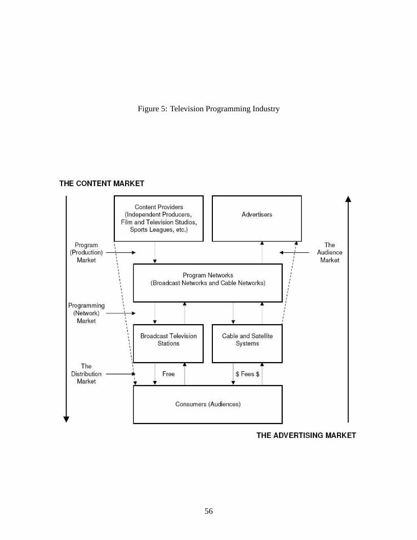
Figure 5: Television Programming Industry

56

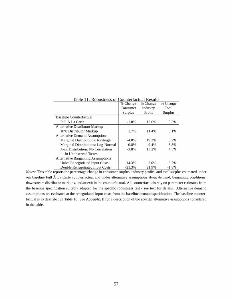
Table 11: Robustness of Counterfactual Results% Change % Change % ChangeConsumer Industry TotalSurplus Profit Surplus

Baseline CounterfactualFull À La Carte -1.0% 13.0% 5.3%

Alternative Distributor Markup10% Distributor Markup 1.7% 11.4% 6.1%

Alternative Demand AssumptionsMarginal Distributions: Rayleigh -4.8% 19.2% 5.2%Marginal Distributions: Log-Normal -0.8% 9.4% 3.8%Joint Distribution: No Correlation -3.8% 13.2% 4.3%

in Unobserved TastesAlternative Bargaining Assumptions

Halve Renegotiated Input Costs 14.3% 2.0% 8.7%Double Renegotiated Input Costs -21.3% 21.9% -1.8%

Notes:This table reports the percentage change in consumer surplus, industry profits, and total surplus estimated under

our baseline Full À La Carte counterfactual and under alternative assumptions about demand, bargaining conditions,

downstream distributor markups, and/or exit in the counterfactual. All counterfactuals rely on parameter estimates from

the baseline specification suitably adapted for the specificrobustness test - see text for details. Alternative demand

assumptions are evaluated at the renegotiated input costs from the baseline demand specification. The baseline counter-

factual is as described in Table 10. See Appendix B for a description of the specific alternative assumptions considered

in the table.

57