electronics

Article

Antenna Design by Means of the Fruit FlyOptimization Algorithm

Lucas Polo-López *,† ID , Juan Córcoles ID and Jorge A. Ruiz-Cruz ID

Department of Electronic and Communication Technology, Universidad Autónoma de Madrid, E-28049 Madrid,Spain; Juan.corcoles@uam.es (J.C.); Jorge.ruizcruz@uam.es (J.A.R.-C.)* Correspondence: lucas.polo@uam.es; Tel.: +34-91-497-7478† C/Francisco Tomás y Valiente 11, Escuela Politécnica Superior, E-28049 Madrid, Spain.

Received: 14 November 2017; Accepted: 29 December 2017; Published: 3 January 2018

Abstract: In this work a heuristic optimization algorithm known as the Fruit fly Optimization Algorithmis applied to antenna design problems. The original formulation of the algorithm is presented and it isadapted to array factor and horn antenna optimization problems. Specifically, it is applied to the arrayfactor synthesis of uniformly-fed, non-equispaced arrays and to the profile optimization of multimodehorn antennas. Several numerical examples are presented and the obtained results are compared withthose provided by a deterministic optimization based on a simplex method and another well-knownheuristic approach, the Genetic Algorithm.

Keywords: antenna; global optimization; horn design

1. Introduction

The design of microwave and millimetre-wave devices is tightly related to optimization processes.In the first stages of the design process a circuital approximation of the problem may be used in somecases (e.g., filters, couplers, etc.), and the parameters of this circuit can be optimized to obtain an initialdesign of the device. Nevertheless, these approximations do not take complex electromagnetic effectsinto account. Therefore, in complex designs an optimization of a proper full-wave model of the deviceis necessary to fine tune the main parameters of the device and obtain the final design.

Many optimization processes are based on deterministic routines that traditionally make use ofthe derivatives of a certain cost function. Nevertheless, modern computational power allows the use ofheuristic or evolutionary techniques such as the Genetic Algorithm (GA) [1–5], Ant Colony Optimization(ACO) [6–8], Particle Swarm Optimization (PSO) [9–12], or Gravitational Search Algorithm (GSA) [13,14]among others. These algorithms are especially suited for problems where the derivative of the costfunction is unknown or not easily computed. Additionally, they are also less prone to get stuck at a localminima of the cost function than the techniques based on derivatives.

In this work, one of these algorithms, known as the Fruit fly Optimization Algorithm (FOA) [15],is presented and adapted for its application to the design of antenna devices. This algorithm wascreated to study financial distress models [15] and it has also been successfully applied to otherproblems [16,17]. Nevertheless, the application of this algorithm to antenna design optimization hasbeen very limited; few examples exist in the literature [18,19] and all of them are dedicated to thesynthesis of array factor analytical functions.

To illustrate the performance of the implemented algorithm different numerical examples arepresented. Specifically, the FOA will be first applied to the problem of synthesizing an array factor(as an initial validation example) and then to the more complex case of the optimization of horn antennaprofiles, which are of primary interest in the front-end of modern communication systems [3,4]. To thebest of the authors’ knowledge the FOA has not been applied to complex radiation problems like these,which require full wave simulations.

Electronics 2018, 7, 3; doi:10.3390/electronics7010003 www.mdpi.com/journal/electronics

Electronics 2018, 7, 3 2 of 14

2. Description of the Algorithm

The FOA is based on the food searching behaviour of a swarm of fruit flies. These insects arecapable of finding food kilometres away from their location by using two mechanisms: osphresis andvision. The osphresis organs of each fly in a swarm can smell all types of scents and make each flymove according to its osphresis sensing. Then, after each fly gets close to the estimated food locationfollowing its own smell concentration judgement, the whole swarm moves by using vision towardsthe fly whose location provides the actual highest smell concentration of food [15].

The computational implementation of the algorithm repeats this process for a defined number ofiterations. The flies move in a two-dimensional space with coordinates X and Y, and the parameters tobe optimized are related to the smell concentration judgement of each fly.

Consequently, in each iteration of the FOA, the following steps must be carried out:

• The swarm is positioned at the location (X(0); Y(0)), with a given smell concentration Smell(0).For each fly i in the swarm:

1. The fly moves around a random distance, searching for food by using the osphresis:

X(i) = X(0) + RX , Y(i) = Y(0) + RY, (1)

where RX and RY are random values.

2. The smell concentration judgement value is defined as the reciprocal of the distance to theorigin of coordinates:

S(i) =1√

(X(i))2 + (Y(i))2(2)

3. Compute the smell concentration of the fly’s current location by using the smell concentrationfunction (equivalent to a fitness function):

Smell(i) = Function(S(i)) (3)

• Look for the specific fly I with the best smell concentration. If this value is better than the valuein the initial location of the swarm (X(0); Y(0)) then move the swarm towards the position of thefly I by using the vision sense:

X(0) = X(I), Y(0) = Y(I) (4)

The described behaviour of the algorithm is represented in Figure 1.

(0; 0)

𝐹𝐹𝐹𝐹𝐹𝐹 𝑓𝑓𝐹𝐹𝑓𝑓𝑓𝑓𝑓𝑓𝑋𝑋(0);𝑌𝑌(0)

𝐹𝐹𝐹𝐹𝐹𝐹 1𝑋𝑋(1);𝑌𝑌(1)

𝐹𝐹𝐹𝐹𝐹𝐹 2𝑋𝑋(2);𝑌𝑌(2)

𝐹𝐹𝐹𝐹𝐹𝐹 3𝑋𝑋(3);𝑌𝑌(3)

Food𝐼𝐼𝐼𝐼𝐼𝐼𝐼𝐼𝐼𝐼𝐼𝐼𝐼𝐼𝐼𝐼𝐼𝐼 𝐼𝐼𝐼𝐼𝑓𝑓𝐹𝐹𝑒𝑒𝐼𝐼𝐼𝐼𝑓𝑓𝑒𝑒

𝑥𝑥 𝐴𝐴𝑥𝑥𝐼𝐼𝐴𝐴

y𝐴𝐴𝑥𝑥𝐼𝐼𝐴𝐴

Figure 1. Schematic representation of the FOA behaviour.

In order to guarantee that the FOA converges, and that this convergence is reached in a reasonableamount of time, two important factors must be considered: the initial positions of the fly swarms andthe generation of the random values RX and RY.

Electronics 2018, 7, 3 3 of 14

The swarm positions could be initialized randomly, but a significantly faster convergence can beachieved by using some prior knowledge of the problem, as it is typical with heuristic algorithms, andmanually initializing them to values in the range of the solution values, making a rough approximation.

The random values RX and RY are generated using a uniform distribution. The interval of thisdistribution must be chosen carefully since if it is very big the search will be erratic and the algorithmwill have trouble converging to a maximum. On the other hand, if it is too small the search will be veryslow and, in addition, the risk of getting stuck in a local maximum of the smell function (equivalent toa minimum of a cost function) will be larger.

As it happens with most of these heuristic techniques, this FOA description may recall to anotheralgorithm of this family like, in this case, the PSO. Nevertheless, it is worth mentioning that despitetheir similarities there are usually subtle but relevant differences between these algorithms. As anexample, the particles of PSO present inertia, whereas the flies of FOA do not.

3. Numerical Examples

3.1. Application to Array Factor Synthesis

As an initial proof of concept the implemented FOA has been applied to the problem of optimizingan array factor. This example has been chosen since the evaluation of the required smell function is notcomputationally expensive and therefore it allows for a faster testing of the implemented algorithm.In the next section a problem with a more sophisticated smell function will be presented.

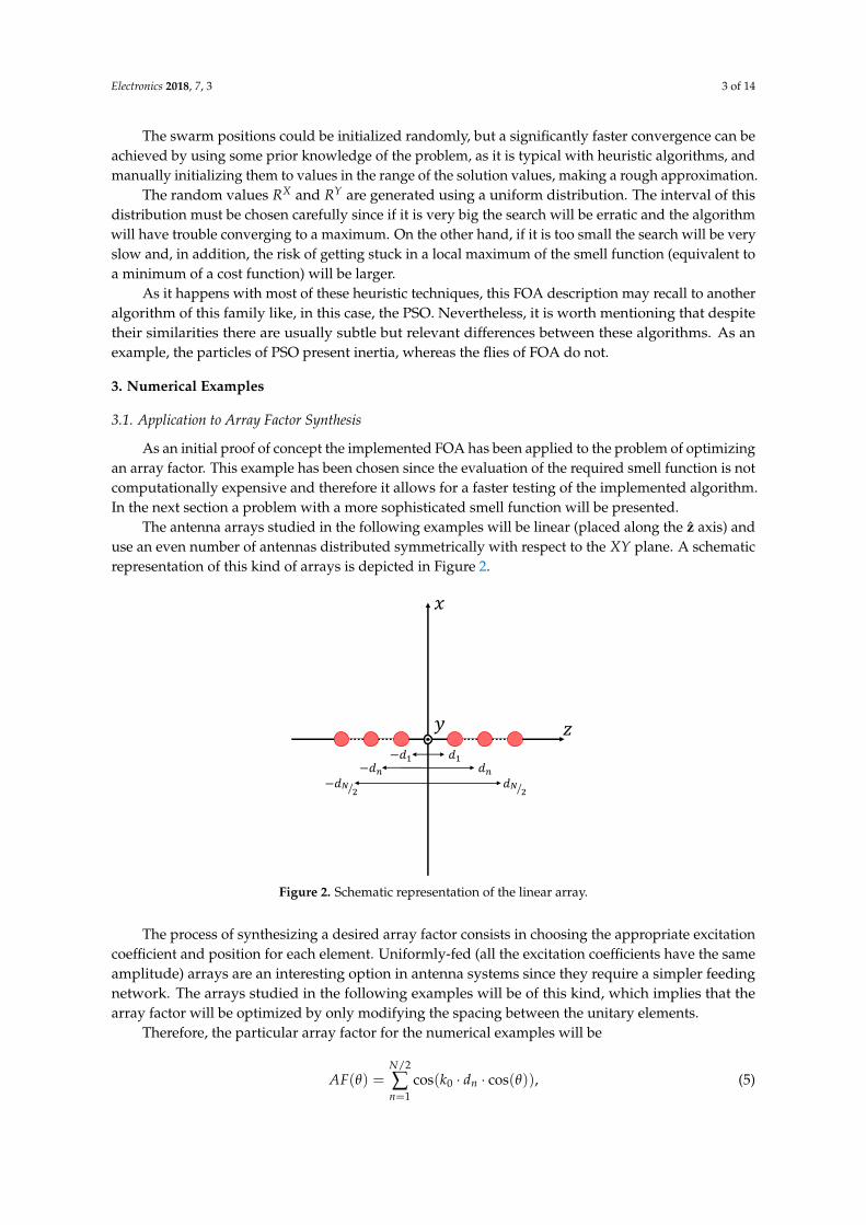
The antenna arrays studied in the following examples will be linear (placed along the z axis) anduse an even number of antennas distributed symmetrically with respect to the XY plane. A schematicrepresentation of this kind of arrays is depicted in Figure 2.

𝑦

𝑥

𝑧𝑑1

𝑑𝑛𝑑 ൗ𝑁 2

−𝑑1−𝑑𝑛

−𝑑 ൗ𝑁 2

Figure 2. Schematic representation of the linear array.

The process of synthesizing a desired array factor consists in choosing the appropriate excitationcoefficient and position for each element. Uniformly-fed (all the excitation coefficients have the sameamplitude) arrays are an interesting option in antenna systems since they require a simpler feedingnetwork. The arrays studied in the following examples will be of this kind, which implies that thearray factor will be optimized by only modifying the spacing between the unitary elements.

Therefore, the particular array factor for the numerical examples will be

AF(θ) =N/2

∑n=1

cos(k0 · dn · cos(θ)), (5)

Electronics 2018, 7, 3 4 of 14

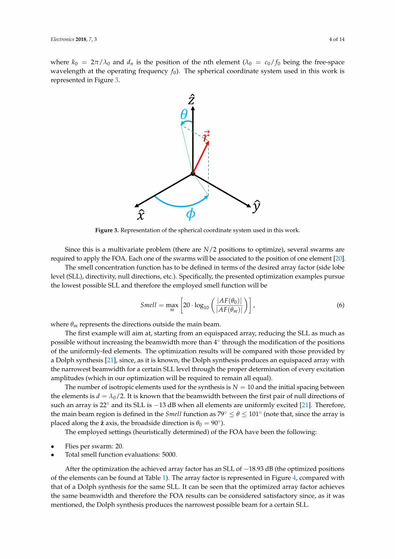
where k0 = 2π/λ0 and dn is the position of the nth element (λ0 = c0/ f0 being the free-spacewavelength at the operating frequency f0). The spherical coordinate system used in this work isrepresented in Figure 3.

ො𝑥

Ƹ𝑧

𝜙

𝜃

Ԧ𝑟

ො𝑦

Figure 3. Representation of the spherical coordinate system used in this work.

Since this is a multivariate problem (there are N/2 positions to optimize), several swarms arerequired to apply the FOA. Each one of the swarms will be associated to the position of one element [20].

The smell concentration function has to be defined in terms of the desired array factor (side lobelevel (SLL), directivity, null directions, etc.). Specifically, the presented optimization examples pursuethe lowest possible SLL and therefore the employed smell function will be

Smell = maxm

[20 · log10

(|AF(θ0)||AF(θm)|

)], (6)

where θm represents the directions outside the main beam.The first example will aim at, starting from an equispaced array, reducing the SLL as much as

possible without increasing the beamwidth more than 4◦ through the modification of the positionsof the uniformly-fed elements. The optimization results will be compared with those provided bya Dolph synthesis [21], since, as it is known, the Dolph synthesis produces an equispaced array withthe narrowest beamwidth for a certain SLL level through the proper determination of every excitationamplitudes (which in our optimization will be required to remain all equal).

The number of isotropic elements used for the synthesis is N = 10 and the initial spacing betweenthe elements is d = λ0/2. It is known that the beamwidth between the first pair of null directions ofsuch an array is 22◦ and its SLL is −13 dB when all elements are uniformly excited [21]. Therefore,the main beam region is defined in the Smell function as 79◦ ≤ θ ≤ 101◦ (note that, since the array isplaced along the z axis, the broadside direction is θ0 = 90◦).

The employed settings (heuristically determined) of the FOA have been the following:

• Flies per swarm: 20.• Total smell function evaluations: 5000.

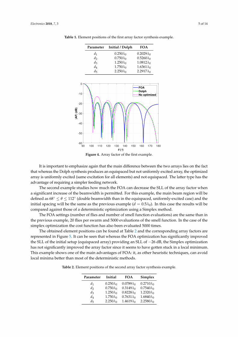
After the optimization the achieved array factor has an SLL of −18.93 dB (the optimized positionsof the elements can be found at Table 1). The array factor is represented in Figure 4, compared withthat of a Dolph synthesis for the same SLL. It can be seen that the optimized array factor achievesthe same beamwidth and therefore the FOA results can be considered satisfactory since, as it wasmentioned, the Dolph synthesis produces the narrowest possible beam for a certain SLL.

Electronics 2018, 7, 3 5 of 14

Table 1. Element positions of the first array factor synthesis example.

Parameter Initial / Dolph FOA

d1 0.250λ0 0.2029λ0d2 0.750λ0 0.5260λ0d3 1.250λ0 1.0812λ0d4 1.750λ0 1.6361λ0d5 2.250λ0 2.2917λ0

90 100 110 120 130 140 150 160 170 180

(°)

-60

-50

-40

-30

-20

-10

0

|AF

| (d

B)

FOA

Dolph

No optimized

Figure 4. Array factor of the first example.

It is important to emphasize again that the main difference between the two arrays lies on the factthat whereas the Dolph synthesis produces an equispaced but not uniformly excited array, the optimizedarray is uniformly excited (same excitation for all elements) and not equispaced. The latter type has theadvantage of requiring a simpler feeding network.

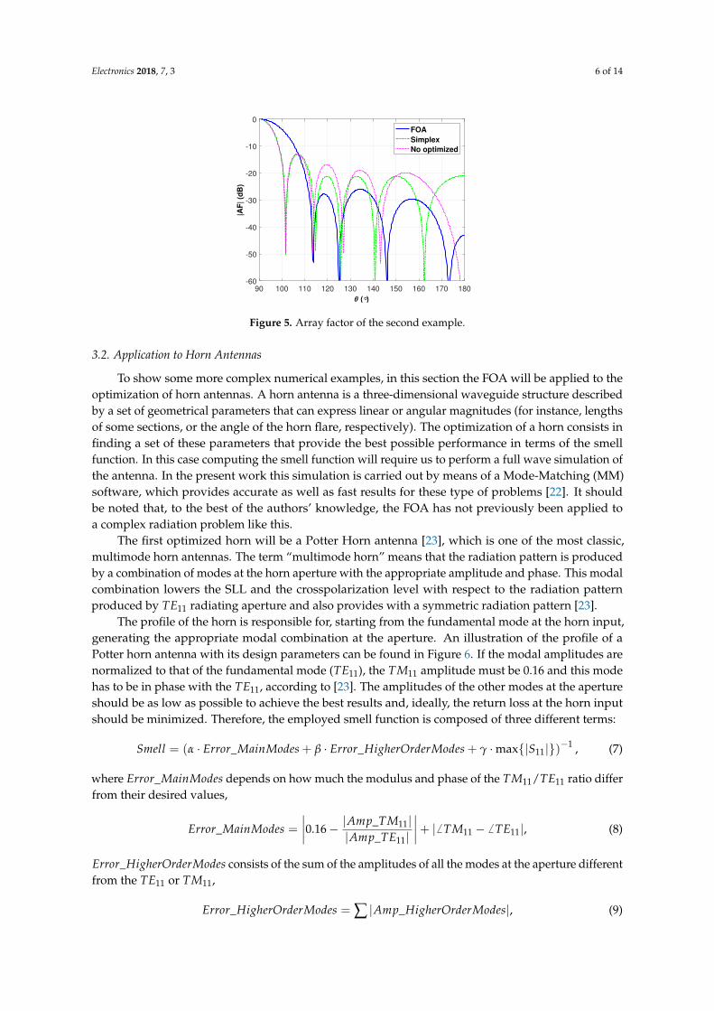
The second example studies how much the FOA can decrease the SLL of the array factor whena significant increase of the beamwidth is permitted. For this example, the main beam region will bedefined as 68◦ ≤ θ ≤ 112◦ (double beamwidth than in the equispaced, uniformly-excited case) and theinitial spacing will be the same as the previous example (d = 0.5λ0). In this case the results will becompared against those of a deterministic optimization using a Simplex method.

The FOA settings (number of flies and number of smell function evaluations) are the same than inthe previous example, 20 flies per swarm and 5000 evaluations of the smell function. In the case of thesimplex optimization the cost function has also been evaluated 5000 times.

The obtained element positions can be found at Table 2 and the corresponding array factors arerepresented in Figure 5. It can be seen that whereas the FOA optimization has significantly improvedthe SLL of the initial setup (equispaced array) providing an SLL of −26 dB, the Simplex optimizationhas not significantly improved the array factor since it seems to have gotten stuck in a local minimum.This example shows one of the main advantages of FOA: it, as other heuristic techniques, can avoidlocal minima better than most of the deterministic methods.

Table 2. Element positions of the second array factor synthesis example.

Parameter Initial FOA Simplex

d1 0.250λ0 0.0789λ0 0.2710λ0d2 0.750λ0 0.3149λ0 0.7540λ0d3 1.250λ0 0.8228λ0 1.2320λ0d4 1.750λ0 0.7631λ0 1.6840λ0d5 2.250λ0 1.4619λ0 2.2580λ0

Electronics 2018, 7, 3 6 of 14

90 100 110 120 130 140 150 160 170 180

(°)

-60

-50

-40

-30

-20

-10

0

|AF

| (d

B)

FOA

Simplex

No optimized

Figure 5. Array factor of the second example.

3.2. Application to Horn Antennas

To show some more complex numerical examples, in this section the FOA will be applied to theoptimization of horn antennas. A horn antenna is a three-dimensional waveguide structure describedby a set of geometrical parameters that can express linear or angular magnitudes (for instance, lengthsof some sections, or the angle of the horn flare, respectively). The optimization of a horn consists infinding a set of these parameters that provide the best possible performance in terms of the smellfunction. In this case computing the smell function will require us to perform a full wave simulation ofthe antenna. In the present work this simulation is carried out by means of a Mode-Matching (MM)software, which provides accurate as well as fast results for these type of problems [22]. It shouldbe noted that, to the best of the authors’ knowledge, the FOA has not previously been applied toa complex radiation problem like this.

The first optimized horn will be a Potter Horn antenna [23], which is one of the most classic,multimode horn antennas. The term “multimode horn” means that the radiation pattern is producedby a combination of modes at the horn aperture with the appropriate amplitude and phase. This modalcombination lowers the SLL and the crosspolarization level with respect to the radiation patternproduced by TE11 radiating aperture and also provides with a symmetric radiation pattern [23].

The profile of the horn is responsible for, starting from the fundamental mode at the horn input,generating the appropriate modal combination at the aperture. An illustration of the profile of aPotter horn antenna with its design parameters can be found in Figure 6. If the modal amplitudes arenormalized to that of the fundamental mode (TE11), the TM11 amplitude must be 0.16 and this modehas to be in phase with the TE11, according to [23]. The amplitudes of the other modes at the apertureshould be as low as possible to achieve the best results and, ideally, the return loss at the horn inputshould be minimized. Therefore, the employed smell function is composed of three different terms:

Smell = (α · Error_MainModes + β · Error_HigherOrderModes + γ ·max{|S11|})−1 , (7)

where Error_MainModes depends on how much the modulus and phase of the TM11/TE11 ratio differfrom their desired values,

Error_MainModes =∣∣∣∣0.16− |Amp_TM11|

|Amp_TE11|

∣∣∣∣+ | 6 TM11 − 6 TE11|, (8)

Error_HigherOrderModes consists of the sum of the amplitudes of all the modes at the aperture differentfrom the TE11 or TM11,

Error_HigherOrderModes = ∑ |Amp_HigherOrderModes|, (9)

Electronics 2018, 7, 3 7 of 14

S11 is the reflection coefficient of the fundamental mode at the input waveguide and α, β, γ areweighting coefficients to balance the three different terms. The modal amplitudes have to be evaluatedat the design frequency which for this design will be 94 GHz.

Figure 6. Representation of the Potter horn profile.

The optimization of the parameters represented in Figure 6 must maximize the smell function in (7).The step from r2 to r3 is responsible for generating the TM11 mode with the appropriate amplitude and,by varying the length L2, the correct phasing between the two modes can be adjusted. The step betweenr1 and r2 is used just to achieve a better return loss value, since the value of r2 is bounded to only allowthe propagation of the fundamental mode. Finally, the flaring angle θ is chosen around 6.5◦ but its finalvalue must be optimized depending on the values chosen for the rest of the design parameters.

Since this is a well known problem there are some design formulas in the literature that can beused to obtain a first approximation of the horn profile [23]. The values provided by these formulasare used as a starting point for the optimization and can be found in Table 3.

Table 3. Values of the Potter horn design parameters obtained by different methods.

Parameter Initial FOA Simplex

r2 1.50 mm 1.70 mm 1.64 mmL2 1.60 mm 6.11 mm 2.78 mmr3 1.95 mm 2.44 mm 2.13 mmL3 3.99 mm 2.64 mm 2.76 mmθ 6.5◦ 5.29◦ 7.72◦

The FOA is configured to use 40 flies per swarm and to evaluate the smell function just 3000 times(this same constraint is also used for the simplex method). Additionally the maximum variation rangefor each parameter in a single iteration is configured as following:

• Radii: 0.15 mm• Lengths: 0.15 · λ0• Angle: 0.25◦

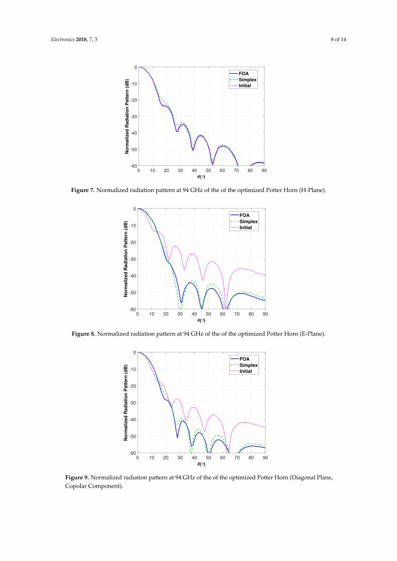
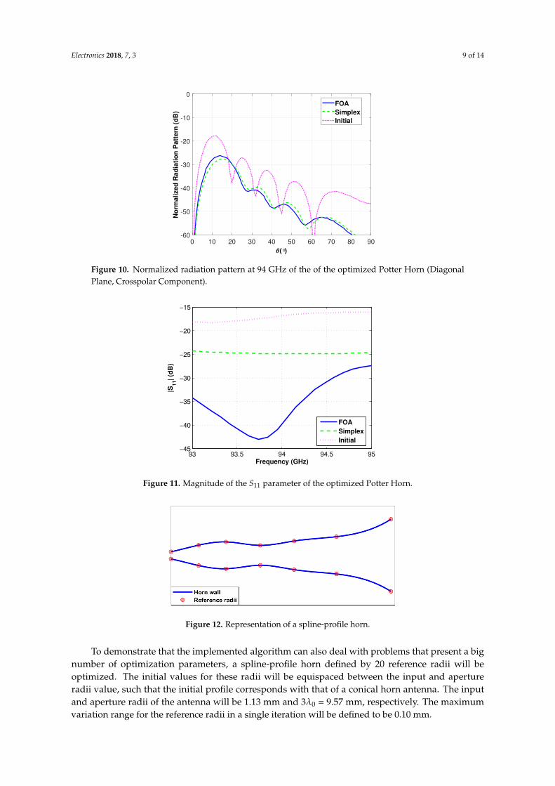
After the optimization, by means of the FOA and the simplex method, the resultant designparameters are the ones presented in Table 3. The different components of the radiation pattern can befound in Figures 7–10. The magnitude of the S11 parameter is represented in Figure 11.

It can be seen that the design provided by the FOA is slightly better in terms of SLL and beamsymmetry, and it also presents a significantly better return loss.

The second horn that will be studied is a spline-profile horn. This is another type of multimodehorn that uses a smooth varying profile (instead of using steps or corrugations) to achieve a certainmode combination at its aperture [24]. The profile of one of these antennas is defined by the splinecurve that passes across a set of reference radii, as illustrated in Figure 12. Therefore by correctlyvarying the value of these radii the modal combination at the aperture can be adjusted.

Electronics 2018, 7, 3 8 of 14

0 10 20 30 40 50 60 70 80 90

(°)

-60

-50

-40

-30

-20

-10

0

No

rmalized

Rad

iati

on

Patt

ern

(d

B)

FOA

Simplex

Initial

Figure 7. Normalized radiation pattern at 94 GHz of the of the optimized Potter Horn (H-Plane).

0 10 20 30 40 50 60 70 80 90

(°)

-60

-50

-40

-30

-20

-10

0

No

rmalized

Rad

iati

on

Patt

ern

(d

B)

FOA

Simplex

Initial

Figure 8. Normalized radiation pattern at 94 GHz of the of the optimized Potter Horn (E-Plane).

0 10 20 30 40 50 60 70 80 90

(°)

-60

-50

-40

-30

-20

-10

0

No

rmalized

Rad

iati

on

Patt

ern

(d

B)

FOA

Simplex

Initial

Figure 9. Normalized radiation pattern at 94 GHz of the of the optimized Potter Horn (Diagonal Plane,Copolar Component).

Electronics 2018, 7, 3 9 of 14

0 10 20 30 40 50 60 70 80 90

(°)

-60

-50

-40

-30

-20

-10

0

No

rmalized

Rad

iati

on

Patt

ern

(d

B)

FOA

Simplex

Initial

Figure 10. Normalized radiation pattern at 94 GHz of the of the optimized Potter Horn (DiagonalPlane, Crosspolar Component).

93 93.5 94 94.5 95−45

−40

−35

−30

−25

−20

−15

Frequency (GHz)

|S1

1|

(dB

)

FOA

Simplex

Initial

Figure 11. Magnitude of the S11 parameter of the optimized Potter Horn.

Figure 12. Representation of a spline-profile horn.

To demonstrate that the implemented algorithm can also deal with problems that present a bignumber of optimization parameters, a spline-profile horn defined by 20 reference radii will beoptimized. The initial values for these radii will be equispaced between the input and apertureradii value, such that the initial profile corresponds with that of a conical horn antenna. The inputand aperture radii of the antenna will be 1.13 mm and 3λ0 = 9.57 mm, respectively. The maximumvariation range for the reference radii in a single iteration will be defined to be 0.10 mm.

Electronics 2018, 7, 3 10 of 14

The same smell function used for the optimization of the Potter Horn antenna, (7), will be usedin this design since it provides with a good mode combination to increase directivity and decreasethe crosspolarisation level. The resultant radiation pattern after the FOA optimization can be foundin Figure 13, where it can be seen that it presents a crosspolarisation level significantly lower than−20 dB and a good main beam symmetry. The S11 is illustrated in Figure 14, revealing a value lowerthan −30 dB for the band of interest.

0 10 20 30 40 50 60 70 80 90

(°)

-60

-50

-40

-30

-20

-10

0N

orm

alize

d R

ad

iati

on

Pa

tte

rn (

dB

) =0°

=90°

=45° (Cop)

=45° (Cxp)

Figure 13. Normalized radiation pattern at 94 GHz of the of the optimized spline-profile horn.

93 93.5 94 94.5 95

Frequency (GHz)

-35

-30

-25

-20

-15

-10

-5

0

|S11|

(dB

)

Figure 14. Magnitude of the S11 parameter of the optimized spline-profile horn.

3.3. Statistical Analysis of the Results

One of the drawbacks of heuristic optimization techniques is that, because of its random nature,the results may not always be the same for different realizations. Therefore obtaining a good result fora certain optimization problem does not guarantee that the algorithm gives, in general, good resultsfor that problem.

To asses this, a statistical study of the FOA performance has been carried out. This study consistedin performing 100 optimizations of the already presented Potter horn and then analysing the obtainedsmell values to compare them with the results achieved by the simplex method. In both cases (FOAand Simplex) the number of cost function evaluations has been set to 3000.

Electronics 2018, 7, 3 11 of 14

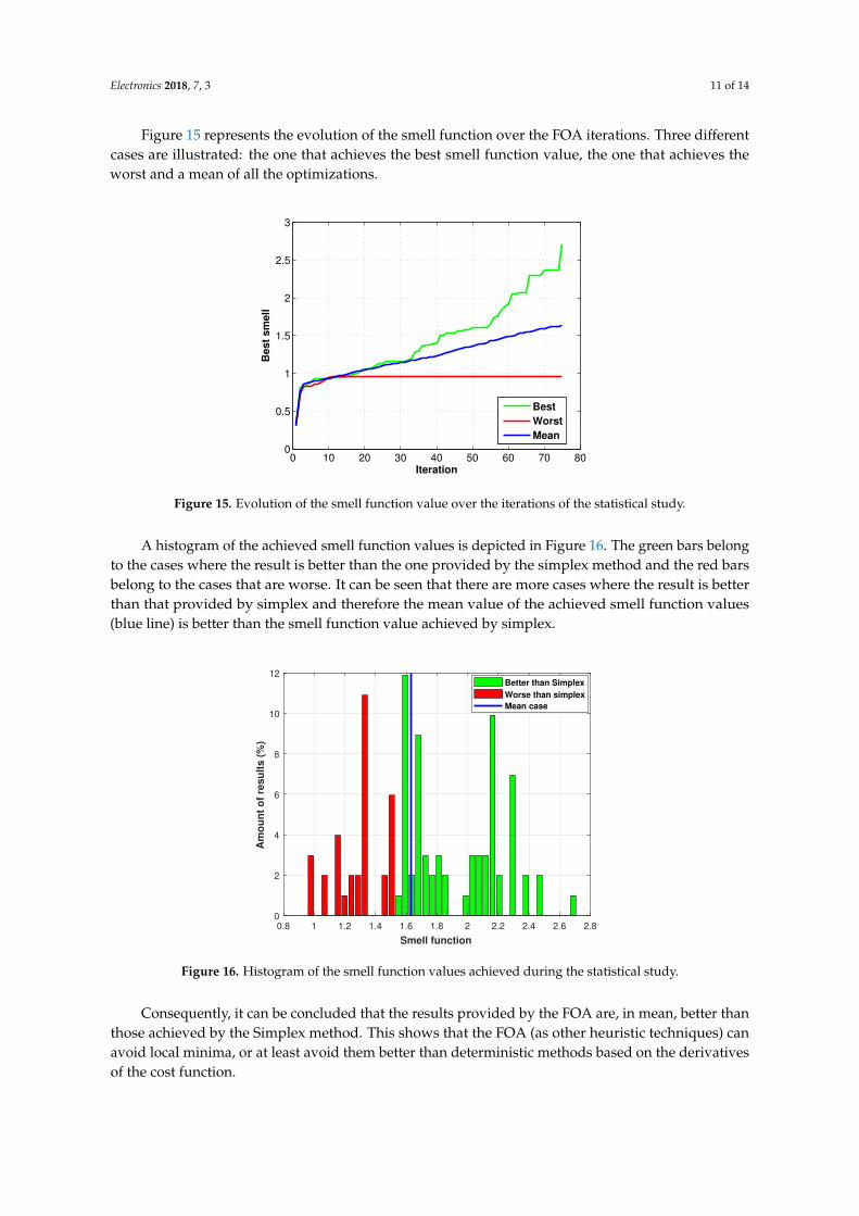
Figure 15 represents the evolution of the smell function over the FOA iterations. Three differentcases are illustrated: the one that achieves the best smell function value, the one that achieves theworst and a mean of all the optimizations.

0 10 20 30 40 50 60 70 800

0.5

1

1.5

2

2.5

3

Iteration

Be

st

sm

ell

Best

Worst

Mean

Figure 15. Evolution of the smell function value over the iterations of the statistical study.

A histogram of the achieved smell function values is depicted in Figure 16. The green bars belongto the cases where the result is better than the one provided by the simplex method and the red barsbelong to the cases that are worse. It can be seen that there are more cases where the result is betterthan that provided by simplex and therefore the mean value of the achieved smell function values(blue line) is better than the smell function value achieved by simplex.

0.8 1 1.2 1.4 1.6 1.8 2 2.2 2.4 2.6 2.8

Smell function

0

2

4

6

8

10

12

Am

ou

nt

of

resu

lts (

%)

Better than Simplex

Worse than simplex

Mean case

Figure 16. Histogram of the smell function values achieved during the statistical study.

Consequently, it can be concluded that the results provided by the FOA are, in mean, better thanthose achieved by the Simplex method. This shows that the FOA (as other heuristic techniques) canavoid local minima, or at least avoid them better than deterministic methods based on the derivativesof the cost function.

Electronics 2018, 7, 3 12 of 14

3.4. Comparison with a Genetic Algorithm

As a final test, results from the FOA have been compared with the ones provided by anotherheuristic method, the Genetic Algorithm (GA), specifically with its commercial implementationprovided by Matlab [25].

The initial population of the GA has been initialized to the same value used as a starting point forthe FOA optimization. Since the used implementation of the GA does not allow us to set the maximumvariation range of each parameter for every single iteration, global upper/lower boundaries have beenprovided for the design parameters to be optimized. This is done in order to prevent the GA fromachieving unrealistic values. These boundaries (presented in Table 4) have been chosen based on thebest design provided by the FOA, with an increased interval to allow the GA to find a better maximumfor the smell function.

Table 4. Boundaries for the design parameters during the Genetic Algorithm optimization.

Parameter Lower Boundary Upper Boundary

r2 1.13 mm 9.57 mmL2 1.00 mm 10.00 mmr3 1.13 mm 9.57 mmL3 1.00 mm 10.00 mmθ 2.0◦ 10.0◦

Figure 17 shows two histograms representing the distribution of smell function values obtained byboth algorithms. It can be seen that the FOA results are similar to those of the GA for the Potter Horndesign. It should be borne in mind that a rigorous global comparison would require the analysis ofa larger span of application problems, which is beyond the scope of this paper (focused on presentingthe FOA and its application to antenna design). Overall, it can be concluded that the performance ofthe implemented algorithm for this problem is comparable to that of other heuristic algorithms likethe commercial implementation of the GA.

0.5 1 1.5 2 2.5 3 3.5

Smell value

0

2

4

6

8

10

12

14

Am

ou

nt

of

res

ult

s (

%)

FOA

GA

Figure 17. Comparison of the results provided by the implemented FOA and a commercial implementationof a GA. SmellFOA = 1.73, σFOA = 0.41, SmellGA = 1.71, σGA = 0.49. Mean value (Smellx) and variance (σx)of the Smell function results.

Electronics 2018, 7, 3 13 of 14

4. Conclusions

In the present work an algorithm for heuristic optimization known as the Fruit fly OptimizationAlgorithm (FOA) has been presented. The original algorithm has been adapted for its application totwo different antenna design problems: array factor synthesis and design of horn antennas.

To illustrate the usefulness of the implemented algorithm different numerical examples havebeen presented. The FOA has been used to synthesize two uniformly-fed, non-equispaced arrays withminimum SLL parting from an equispaced array. Additionally, two horns have been optimized withvery good results. The optimization of these antennas required to perform a full wave simulation of thedevice (which was done using a Mode-Matching software) to compute the smell function, validatingthe use of this algorithm in complex electromagnetic problems..

In both cases the FOA results were compared with a deterministic optimization (based ona Simplex method), which obtained worse results since it kept getting stuck in a local minima. Finally,a small statistical study in which the FOA results were compared not only with a simplex algorithmbut also with a Genetic Algorithm has been presented. All these studies show that the FOA is a veryuseful optimization tool for challenging antenna designs in microwave and millimetre-wave systems.

Acknowledgments: This work was supported by contracts TEC2016-76070-C3-1-R (AEI/FEDER, UE) andS2013/ICE-3000 (Comunidad de Madrid).

Author Contributions: All authors contributed to the development of the code for the full-wave analyses and theoptimization algorithm. L. Polo-López made the final simulations and graphs for the paper, revised by J. Córcolesand J.A. Ruiz-Cruz.

Conflicts of Interest: The authors declare no conflict of interest.

Abbreviations

The following abbreviations are used in this manuscript:

FOA Fruit fly Optimization AlgorithmSLL Side Lobe LevelTE Transverse ElectricTM Transverse MagneticGA Genetic Algorithm

References

1. Haupt, R.L.; Menozzi, J.J.; McCormack, C.J. Thinned arrays using genetic algorithms. In Proceedings of theIEEE Antennas and Propagation Society International Symposium, Ann Arbor, MI, USA, 28 June–2 July 1993;Volume 2, pp. 712–715.

2. Johnson, J.M.; Rahmat-Samii, V. Genetic algorithms in engineering electromagnetics. IEEE Antennas Propag. Mag.1997, 39, 7–21.

3. Ares-Pena, F.J.; Rodriguez-Gonzalez, J.A.; Villanueva-Lopez, E.; Rengarajan, S.R. Genetic algorithms in thedesign and optimization of antenna array patterns. IEEE Trans. Antennas Propag. 1999, 47, 506–510.

4. Dey, R.; Chakrabarty, S.; Jyoti, R.; Kurian, T. Synthesis and analysis of multi-mode profile horn using modematching technique and evolutionary algorithm. IET Microw. Antennas Propag. 2016, 10, 276–282.

5. Rolland, A.; Ettorre, M.; Drissi, M.; Coq, L.L.; Sauleau, R. Optimization of Reduced-Size Smooth-WalledConical Horns Using BoR-FDTD and Genetic Algorithm. IEEE Trans. Antennas Propag. 2010, 58, 3094–3100.

6. Quevedo-Teruel, O.; Rajo-Iglesias, E. Ant Colony Optimization in Thinned Array Synthesis With MinimumSidelobe Level. IEEE Antennas Wirel. Propag. Lett. 2006, 5, 349–352.

7. Mosca, S.; Ciattaglia, M. Ant Colony Optimization to Design Thinned Arrays. In Proceedings of the 2006IEEE Antennas and Propagation Society International Symposium, Albuquerque, NM, USA, 9–14 July 2006;pp. 4675–4678.

8. Rajo-Iglesias, E.; Quevedo-Teruel, O. Linear array synthesis using an ant-colony-optimization-based algorithm.IEEE Antennas Propag. Mag. 2007, 49, 70–79.

Electronics 2018, 7, 3 14 of 14

9. Khodier, M.M.; Christodoulou, C.G. Linear array geometry synthesis with minimum sidelobe level and nullcontrol using particle swarm optimization. IEEE Trans. Antennas Propag. 2005, 53, 2674–2679.

10. Donelli, M.; Martini, A.; Massa, A. A Hybrid Approach Based on PSO and Hadamard Difference Sets for theSynthesis of Square Thinned Arrays. IEEE Trans. Antennas Propag. 2009, 57, 2491–2495.

11. Robinson, J.; Sinton, S.; Rahmat-Samii, Y. Particle swarm, genetic algorithm, and their hybrids: Optimizationof a profiled corrugated horn antenna. In Proceedings of the IEEE Antennas and Propagation SocietyInternational Symposium (IEEE Cat. No.02CH37313), San Antonio, TX, USA, 16–21 June 2002; Volume 1,pp. 314–317.

12. Moradi, A.; Mohajeri, F. Reduction of SLL in a square horn antenna in presence of metamaterial surfacesby using of particle swarm optimization. In Proceedings of the 2016 24th Iranian Conference on ElectricalEngineering (ICEE), Shiraz, Iran, 10–12 May 2016; pp. 598–603.

13. Rashedi, E.; Nezamabadi-pour, H.; Saryazdi, S. GSA: A Gravitational Search Algorithm. Inf. Sci. 2009, 179,2232–2248.

14. Pelusi, D.; Mascella, R.; Tallini, L. Revised Gravitational Search Algorithms Based on Evolutionary-FuzzySystems. Algorithms 2017, 10, doi:10.3390/a10020044.

15. Pan, W.T. A new Fruit Fly Optimization Algorithm: Taking the financial distress model as an example.Knowl.-Based Syst. 2012, 26, 69–74.

16. Liu, Y.; Wang, X.; Li, Y. A Modified Fruit-Fly Optimization Algorithm aided PID controller designing.In Proceedings of the 10th World Congress on Intelligent Control and Automation, Beijing, China, 6–8 July 2012;pp. 233–238.

17. Li, H.Z.; Guo, S.; Li, C.J.; Sun, J.Q. A hybrid annual power load forecasting model based on generalizedregression neural network with fruit fly optimization algorithm. Knowl.-Based Syst. 2013, 37, 378–387.

18. Mhudtongon, N.; Phongcharoenpanich, C.; Kawdungta, S. Modified Fruit Fly Optimization Algorithm forAnalysis of Large Antenna Array. Int. J. Antennas Propag. 2015, 2015, 124675.

19. Mhudtongon, N.; Phongcharoenpanich, C.; Watanabe, K. Linear antenna synthesis with maximum directivityusing improved fruit fly optimization algorithm. In Proceedings of the 2016 URSI International Symposiumon Electromagnetic Theory (EMTS), Espoo, Finland, 14–18 August 2016; pp. 698–701.

20. Pan, W.T. Fruit Fly Optimization Algorithm (Using MATLAB). 2014. Available online:https://www.mathworks.com/matlabcentral/answers/uploaded_files/20100/Fruit%20Fly%20Optimization%20Algorithm_Second%20Edition.pdf (accessed on 1 February 2014).

21. Stutzman, W.L.; Thiele, G. Antenna Theory and Design; John Wiley & Sons: Hoboken, NJ, USA, 1998.22. Conciauro, G.; Guglielmi, M.; Sorrentino, R. Advanced Modal Analysis: CAD Techniques for Waveguide Components

and Filters; John Wiley & Sons: Hoboken, NJ, USA, 2000.23. Olver, A.; Clarricoats, P.; Kishk, A.; Shafai, L. Microwave Horns and Feeds; Electromagnetic Waves Series; IEE:

London, UK; IEEE: New York, NY, USA, 1994.24. Granet, C.; James, G.L.; Bolton, R.; Moorey, G. A smooth-walled spline-profile horn as an alternative to the

corrugated horn for wide band millimeter-wave applications. IEEE Trans. Antennas Propag. 2004, 52, 848–854.25. MATLAB R2016b; The MathWorks, Inc.: Natick, MA, USA, 2017.

c© 2018 by the authors. Licensee MDPI, Basel, Switzerland. This article is an open accessarticle distributed under the terms and conditions of the Creative Commons Attribution(CC BY) license (http://creativecommons.org/licenses/by/4.0/).