WP/05/16

The Russian Flat Tax Reform

Anna Ivanova, Michael Keen, and Alexander Klemm

© 2005 International Monetary Fund WP/05/16

IMF Working Paper

Fiscal Affairs Department

The Russian Flat Tax Reform

Prepared by Anna Ivanova, Michael Keen, and Alexander Klemm1

January 2005

Abstract

This Working Paper should not be reported as representing the views of the IMF. The views expressed in this Working Paper are those of the author(s) and do not necessarily represent those of the IMF or IMF policy. Working Papers describe research in progress by the author(s) and are published to elicit comments and to further debate.

Russia dramatically reduced its higher rates of personal income tax (PIT) in 2001 establishing a single marginal rate at the low level of 13 percent. In the following year, real revenue from the PIT actually increased by about 26 percent. This ‘flat tax’ experience has attracted much attention (and emulation) among policymakers, making it perhaps the most important tax reform of recent years. But it has been little studied. This paper asks whether the strong revenue performance of the PIT was itself a consequence of this reform, using both macro evidence and, in particular, micro-level data on the experiences of individuals and households affected by the reform to varying degrees. It concludes that there is no evidence of a strong supply side effect of the reform. Compliance, however, did improve quite substantially—by about one third according to our estimates—though it remains unclear whether this was due to the parametric reforms or to accompanying changes in enforcement. JEL Classification Numbers: H24, H26, H31 Keywords: Tax reform; flat tax; tax evasion Author(s) E-Mail Address: aivanova@imf.org; mkeen@imf.org; a.klemm@ifs.org.uk

1 Anna Ivanova and Michael Keen are in the Middle East and Central Asia Department and the Fiscal Affairs Departments of the IMF respectively; Alexander Klemm is with the Institute for Fiscal Studies, London. We thank Richard Blundell, Dale Chua, Gohoon Kwon, Victoria Perry, Ian Preston, John Oddling Smee, David Owen, Carlos Silvani, Stephen Smith, Antonio Spilimbergo, and Victor Thuronyi for comments and suggestions on this work. Views and errors are ours alone, and should not be attributed to the Institute for Fiscal Studies or the International Monetary Fund.

- 2 -

Contents Page I. Introduction........................................................................................................................ 4 II. PIT and the 2001 Tax Reforms.......................................................................................... 6 III. Predictions of Theory......................................................................................................... 9 IV. The PIT Reform in a Wider Context................................................................................ 15 V. Micro Evidence: Data, Methodology, and Hypotheses ................................................... 21 VI Panel Data Results ........................................................................................................... 29 VII. Conclusions...................................................................................................................... 39 Text Tables 1. The PIT Rate Structure Before and After Reform............................................................. 6 2. Social Tax Rate Structure Before and After Reform......................................................... 8 3. General Government Revenues, 1994–2003 ................................................................... 16 4. Analyzing Official Income and Tax Data........................................................................ 18 5. Comparisions of RLMS Sample and Official Data ......................................................... 23 6. PIT Payments at Individual Level, Split by Initial Marginal Tax Rate ........................... 29 7. PIT Payments at Individual Level, Split Between Lower- and Higher-Rate Payers ....................................................................................... 30 8. PIT Payments at Individual Level, Extended Definition of Treatment Group ................ 31 9. Difference-in-Differences Estimators for PIT, Total Tax and Gross Income, at Individual-Level................................................................ 32 10. Difference-in-Differences Estimators for Hours Worked and Wage Rate, at Individual-Level .................................................................... 33 11. Changes in PIT Paid at Household-Level, Treatment and Control Defined on Basis of Reported Income.................................................... 35 12. Changes in PIT Paid at Household-Level, Treatment and Control Defined by Consumption-Based Estimate of Gross Income ............................... 36 13. Difference-in-Differences Estimates for PIT, Total Tax and Declared Income, at Household-Level.......................................................... 37 14. Difference-in-Differences Estimates for Compliance, at Household-Level.................... 38 15. Difference-in-Differences Estimates for Gross Income, at Household-Level................. 38 16. Difference-in-Differences Estimates for Hours Worked and Wage Rate, Household-Level ....................................................................... 39

17. Estimates of the share of the hidden economy in transition countries………………….42

- 3 -

Text Figures 1. Labor Supply Before and After Reform .......................................................................... 12 2. Dynamics of Average Labor Productivity, Output, and Wages ...................................... 20 3. Share of Wages and Net Profits in GDP.......................................................................... 20 4. Marginal Tax Rates (Including Social Taxes) Before and After the Reform.................. 25 Appendix 1. Data .................................................................................................................................. 43 Appendix Tables 18. Cleaning of Individual-Level Data .................................................................................. 45 19. Cleaning of Household-Level Data ................................................................................. 45 Reference ..................................................................................................................................... 46

- 4 -

I. INTRODUCTION

At the start of 2001, Russia unified its marginal rates of personal income taxation—previously at 12, 20, and 30 percent—at the flat rate of just 13 percent.2 Over the next year, revenue from the personal income tax (PIT) increased by about 46 percent: about 26 percent in real terms. As a percentage of GDP, PIT revenues increased by nearly one-fifth. Such a strong revenue performance following a marked reduction of marginal tax rates quickly attracted attention, and emulation, both in the countries of the former Soviet Union and, more recently, elsewhere. Ukraine and Slovakia have adopted “flat taxes”—meaning personal income tax structures with a single positive marginal tax rate, set at a relatively low level—at 12 and 19 percent respectively. Similar reforms have been under consideration in Belarus, Georgia, Guatemala, the Kyrgyz Republic, El Salvador, Paraguay, and Poland.3 The Russian reform has thus become an extraordinarily influential one4—arguably the most important tax reform of the last decade. Given the importance of the reform not only for Russia itself but also for the many countries that have adopted, or are considering adopting, similar measures, it is clearly important also to understand that experience, and the lessons that can appropriately be drawn from it. Did the reform indeed have the strong positive effects on compliance and/or labor supply (especially the former) that its advocates have claimed? Were these effects even so strong that the lower tax rates “paid for themselves”? The purpose of this paper is to address these and related questions, both by taking a macroeconomic perspective on wider revenue developments at this time and, in particular, by using the individual- and household level panel data that is now available in the Russian Longitudinal Monitoring Survey (RLMS), spanning pre- and post-reform periods, to provide a clear assessment of the impact of the reform on tax revenue, work effort, wage rates, and taxpayer compliance. Though it has been much commented on, and admired, the Russian experience has been subject to very little rigorous empirical analysis.5 The only econometric analysis of which we are aware is presented in a series of papers from the Institute for Economies in Transition. 2 Note that this is not a flat tax in the sense of Hall and Rabushka (1995), which is essentially an expenditure tax implemented by combining a rate tax on wage income and a cash flow business tax levied at the same rate. Nevertheless, Rabushka (2003) has spoken positively of the Russian experience.

3 As a variant, Armenia has redesigned its progressive PIT and regressive social insurance schedule so that the combination of the two has a single positive marginal rate.

4 Though Russia has been the most influential exponent of the flat tax, it was not in fact the first: Bolivia has had a single rate of personal income tax since 1986, Estonia adopted such a structure in 1994, as did Latvia in 1995.

5 Informal accounts are provided in IMF (2002) and Chua (2003).

- 5 -

The empirical strategy in this work—as in Sinelnikov-Mourylev et al. (2003),6 for instance—has been to use the RLMS to construct observations at the level of the regions of Russia and ask whether the implied PIT base has increased more in those regions where the weighted average marginal tax rate was most reduced. The conclusion drawn is that there has indeed been a significant effect of this sort, with the authors ultimately attributing about half of the revenue gain to the reduction in marginal rates. Though striking, these results are subject to a number of limitations. It could be the case, for instance, that those regions in which the proportion of incomes subject to the higher rates of tax prior to reform were also systematically those which saw, for some reason, the greatest increase in the incomes of those subject to essentially the same marginal rate before and after reform (and hence also the greatest increase in the tax base). Micro-level panel data need to be available and exploited to identify such possibilities, offering potentially the best basis upon which to assess the implications of the reform. That is the approach pursued here. The concern throughout the analysis here, it should be stressed, is solely with positive aspects of the reform, in terms of its impact on revenue, compliance, and labor supply; we do not attempt to gauge the extent of any efficiency or welfare gains, or to evaluate its distributional impact.7 The structure of the paper is as follows. Section II describes the PIT and (important in understanding its effects) related tax reforms in 2001. Section III briefly reviews the lessons of theory as to the likely effects of the reform, and section IV takes a macro perspective on the assessment of the reform. The main analysis, based on micro panel data, is in Section V, which describes the data and methodology used, and in section VI, which reports results. Section VII concludes.

6 See also Chapter 4 of Glavatskaya and Ser'yanova (2003).

7 Sinelnikov-Mourylev et al. (2003) argue that reduced evasion (and hence higher tax payments) by higher-rate taxpayers actually increased the effective progressivity of the PIT with respect to wage income (while finding no conclusive result for its progressivity with respect to total income).

- 6 -

II. PIT AND THE 2001 TAX REFORMS

The change in the rate structure of the PIT, which took effect on January 1, 2001, are summarized in Table 1.

Table 1: The PIT Rate Structure Before and After Reform

Before Reform (2000) After Reform (2001)

Taxable Income1 Marginal Rate Taxable Income1 Marginal Rate Below 3,168 0 Below 4,800 0

3,168 to 50,000 12 Above 4,800 13

50,000 to 150,000 20

Above 150,000 30

Source: Russian Tax Code, Part II. 1 In Russian rubles.

The threshold level of taxable income at which the higher rates began prior to reform is high: about 187 percent of the average wage in 2000. It should be noted too that although the basic exemption grew by 30 percent in real terms between 2000 and 2001, it remained roughly unchanged relative to the average wage (at about 12 percent).8 Strictly, the post-reform PIT was actually not a single rate tax, since some kinds of income—from gambling, lottery prizes, some insurance payments, from loans at less than market rates and from ‘excessive bank interest9—were taxed at an increased rate of 35 percent in an attempt to close popular avoidance schemes (some of which showed quite considerable adroitness).10 Dividends were taxed at 30 percent (up from 15 percent in 2000). 8 Both before and after reform, this allowance was withdrawn in discrete jumps at higher levels of income (as described in the data appendix). This is taken fully into account in the empirical analysis reported below, but for simplicity ignored in the discussion that follows and in Table 1 and Figure 4.

9 Bank interest became taxable if paid at a rate exceeding 75 percent of the Central Banks’ refinancing rate on ruble deposits or nine percent on foreign currency deposits. Since most deposits earned less than this, interest income was generally untaxed.

10 Under one scheme, for instance, the enterprise purchased insurance against a very low probability event (deducting its premiums). At the same time, its employees entered a contract with the same insurance company for a very high probability event. Employees thus received compensation in the form of an insurance payout, which was not taxable.

- 7 -

There were also changes in 2001 to the base of the PIT, with the elimination of various exclusions for military servicemen and expatriates (such as housing costs, business trips) and the introduction of a simplified system of deductions (standard, social, property and professional). Moreover, there was a modification of the sharing agreement of PIT between federal and regional governments: in 2000 regional governments receive only 80 percent of PIT, from 2001 they received 100 percent. This will have strengthened the collection incentive of regional governments. These changes to the PIT structure were not, however, the only tax reform at this time. Most important for present purposes, Part II of the new tax code also significantly altered the structure of social insurance payments, as shown in Table 2. Prior to the reform, separate contributions were paid to the pension, social, medical and employment funds at a combined rate, at all income levels, of 38.5 percent on the employer and one percent on the employee (the last to the pension fund). After the reform, a single ‘unified social tax’ was charged on the employer—for firms meeting various additional requirements11—at marginal rates decreasing from 35.6 to 5 percent, with the lowest marginal rate applying to salaries in excess of (the very high level of) 600,000 rubles.12 Below 100,000 rubles (about 254 percent of the average wage), the marginal and average rate of the social insurance tax fell by 7.3 points. For those initially paying PIT at the lower rate of 12 percent, the net effect of the 2001 reforms was a reduction in the combined marginal rate of PIT and social insurance of about 1.3 percentage points.13 Several other tax changes also took effect at the start of 2001: • While the combined federal and regional rate of the corporate income tax (CIT)

remained at a maximum of 30 percent,14 local municipalities were allowed to impose a profit tax of up to 5 percent (a power which was used). Thus the combined maximum rose to 35 percent.15

11To qualify for the regressive rate, average payment per employee had to be below a threshold (2500 rubles in 2001) when a certain number of employees with the highest incomes excluded from the calculation. The rationale for this was apparently to encourage compliance on a broad base by denying benefit to firms that declared only a few highly-paid individuals. Moreover, to discourage income shifting, the regressive social scheme in 2001 could be applied only by taking into account average payment per employee in 2000.

12 From 2002 this was reduced further to 2 percent.

13 Because the social taxes are charged on a tax-exclusive basis, this is calculated as the difference between (012+0.01+ 0.385)/(1.385) and (0.13+0.356)/(1.356).

14 Comprising a federal rate of 11 percent plus a regional tax at up to 19 percent.

15 There was also some alignment of the corporate tax bases at the three levels of government. The maximum CIT rate was reduced to 24 percent in 2002 (comprising federal tax at 7.5 percent, regional at between 10.5 and 14.5 percent, and local at up to 2 percent). Investment incentives were also scaled back in 2002 (with preannouncement in 2001) —notably by the removal of investment allowances—and replaced by accelerated

(continued…)

- 8 -

Table 2: Social Tax Rate Structure Before and After Reform 1/

Legal Incidence Before Reform (2000) After Reform (2001)

Income Range Marginal Rate Income Range Marginal Rate

Employee Any 1 Any 0

Employer Any 38.5 2/ Below 100,000 35.6

100,000-300,000 20

300,000-600,000 10

Above 600,000 5 (from 2002: 2)

Source: Russian Tax Code, Part II. 1/ Different rates apply to agricultural workers, lawyers and self-employed. In some regions some additional charges were levied, e.g. in Moscow an Education Levy of one percent. 2/ This made up of contributions to the Pension Fund (28 percent), Social Insurance Fund (5.4), State Employment Fund (1.5), and Medical Insurance Fund (3.6). • The dividend tax was increased, as noted above, but accompanied by the introduction

of a non-refundable credit for underlying CIT paid.16 • The Social Infrastructure Maintenance Tax, effectively a turnover tax at 1.5 percent,

was abolished, and the Road User tax, another turnover tax, was reduced from 2.5 to 1.5 percent.17 There were no changes in the rates of the value added tax,18 but there was some scaling back of exemptions (including a narrowing of the exemption for pharmaceuticals), a shift in mid-year from the origin to the destination basis for trade with other CIS countries (except for trade with Belarus, and on energy), together with the adoption of measures to reduce the compliance burden on small traders.19

depreciation together with a less restrictive regime for the deduction of interest costs (related to capital assets) and other expenses, together with an increase in the length of carry forward from 5 to 10 years.

16 The dividend tax rate was lowered to 6 percent in 2002, when the imputation credit was eliminated.

17 It was abolished at the start of 2003.

18 The basic rate remained at 20 percent, with a reduced rate of 10 percent for basic foodstuffs, children’s’ goods and some other items.

19 Including the adoption of a threshold for compulsory registration of 1 million rubles of sales (in the preceding month).

- 9 -

Tax administration was also undergoing significant change at the time of the PIT reform, as described in Chua (2003). Part I of the new tax code, which became effective on January 1, 1999 in many respects strengthened the legal power of the tax authorities, notably by providing for the introduction of a common taxpayer identification number and allowing, in certain cases, for the indirect assessment of tax liability.20 More authority was also given to the State Tax Service, in particular, in allocating income, deductions and credits across related taxpayers, and in enforcing debt repayments by liquidated companies. Importantly, Part I also eliminated a ceiling on interest accrued on overdue taxes. Some of its provisions, however, worked in the opposite direction: for example, tax obligations were deemed discharged once the taxpayer had provided a payment order to a bank, which allowed taxpayers to claim fulfillment of their obligations without actually paying any tax. Nevertheless, the general thrust of the reform was to strengthen the powers of the tax administration (and further measures to the same effect were taken in 2002)21. How these reforms in the legal framework changed actual practice is harder to judge. There was thus much more going on at the start of 2001 than simply the change in the rate structure of the PIT. One key implication is that it is difficult to isolate effects of the PIT reform alone. The reductions in social insurance taxes, in particular, would be expected to trigger quite similar behavioral responses as the cut in PIT rates, making it especially difficult to disentangle the two.

III. PREDICTIONS OF THEORY

To provide a stylized framework for coming to grips with the anatomy of the 2001 reform, write revenue from the personal income tax, R, as Lw...λτ , where τ denotes the (tax-exclusive) tax rate, λ the ratio of declared taxable income to true taxable income (and so describes the degree of compliance, with 1=λ corresponding to fully truthful reporting), w the gross wage rate and L the level of employment (here abstracting, for simplicity, from capital income components of the PIT base). Denoting proportionate changes by hats, the revenue effect of any reform is then approximated by

.ˆˆˆˆˆ LwR +++≈ λτ (1)

Though some elements of the 2001 PIT reform tended to increase revenue at unchanged behavior, these were relatively minor (the most important probably being the elimination of the exemption for military servicemen). Thus the reform corresponds, for those initially 20 Item 3 of Chapter 91 in Part I of the Tax Code gives the tax authority the power “to assess the tax liability from the data on the taxpayer (or another obligor) available to the tax authority, or by analogy” if access to the taxpayer’s grounds or premises (other than living quarters) is impeded.

21 In particular, the tax police were authorized to conduct tax audits provided a sufficient evidence of a suspected tax crime was available, and to investigate nontax commercial crimes such as money laundering.

- 10 -

paying PIT at a higher rate, to a substantial reduction in τ, amplified by the reduction in social insurance taxes. The question is whether the three types of response to the reform on the right of (1) could have led to such an increase in the tax base as to account, to any substantial degree, for the strong performance of PIT revenue subsequent to the reform. The rest of this section considers each in turn, and considers also the possibility that the reform may have led to some income-shifting between the CIT and PIT.

Gross wage rates

In the formal sector (meaning that in which some tax is paid), one would expect the gross wage w to fall as a consequence of the reduced tax wedge (both PIT and social taxes), reinforcing the direct revenue effect of the tax cut.22 Translated into the terms of the empirical exercise below, the implication is that gross wage rates of groups most affected by the reform should have fallen relative to those of groups less affected. In the informal sector, the gross wage might conceivably have risen (in order to leave take-home wages in line with those available in the formal sector); but this would have had no direct impact on tax revenue.

22 Take, for instance, the natural benchmark case of a competitive labor market, characterized by equality between the demand for labor, D(w)¸ and the supply of labor, S[w(1-λτ)] (taken to depend on the wage net of taxes actually paid, so ignoring for simplicity the risks associated with non-compliance). Denoting the elasticities of labor demand and supply by De and Se (both defined to be positive numbers) it is then routine to show that

)ˆˆ(1

ˆ λτλτ

λτ+⎟

⎠⎞

⎜⎝⎛

−⎟⎟⎠

⎞⎜⎜⎝

⎛

+= DS

S

eeew

so that the gross wage falls unless compliance increases by a greater proportion than the tax rate falls. Using this relationship (and now ignoring, counter-factually but for clarity, the social taxes that would also be expected to affect net wage and hence labor supply), it is straightforward to show that in this simple framework the overall effect on PIT revenue is

)ˆˆ(11

)1(ˆ λτλτ

λτ+

⎥⎥⎦

⎤

⎢⎢⎣

⎡+⎟

⎠⎞

⎜⎝⎛−⎟

⎟⎠

⎞⎜⎜⎝

⎛

+−

= DS

DS

eeeeR .

Thus revenue is more likely to rise (for given )0ˆˆ <+ λτ the greater is the elasticity of demand for labor (indeed a necessary condition for revenue to rise is that this exceed unity), the greater is the elasticity of the supply of labor, the higher is the tax rate and the higher is the initial level of compliance.

- 11 -

Work effort

Effects might be expected from both the change in gross wage rates and the change in the parameters of the PIT and social taxes. The former depends routinely on the elasticity of labor supply, so the latter is the focus here. To simplify, imagine a reform that leaves the exempt amount and starting marginal rate of tax unchanged but lowers, to the same level, the (single) top rate. (In fact, as seen above, the starting marginal rate—inclusive of social insurance—fell by 1.3 percentage points and the pattern of effects at the higher rate was more diverse). As shown in Figure 1, by reducing the higher marginal rate to the level of the standard rate the reform has the effect of rotating the budget constraint relating before- and after-tax income anti-clockwise around the kink point (at the level of income at which that higher rate initially applied) until the budget constraint becomes a straight line. The upper panel of Figure 1 illustrates the impact of this on a taxpayer who pays at higher than the standard rate prior to the reform. The substitution effect of the reform—isolated by comparing the initial choice at a to that which would be made under the hypothetical dashed budget constraint passing through a but parallel to the new budget constraint—is to increase pre-tax income, to a point like b (and hence also to increase the tax base), reflecting the reduction in the marginal tax rate. Acting in the opposite direction, however, is an income effect—represented by the comparison b and the choice that would be made under the post-reform budget constraint—that arises not only from the increase in the marginal wage but also from the increase in net income consequent upon the reduced taxation of intra-marginal income initially taxed at the higher rate. Under the standard assumption that leisure is normal, this tends to reduce work effort, and, hence, the tax base. For an individual who, prior to the reform, locates himself interior to the segment of the budget constraint corresponding to the standard rate it is clear—and so not illustrated—that the reform simply has no effect on work effort or, hence, the tax base. There is, however, another important possibility. The individual shown in the middle panel of the figure locates himself, prior to reform, exactly at the kink point at which the higher rate of tax begins. In this case the reform has only a substitution effect, and work effort increases from that at a to that at a point like b. This may seem an extreme case—though one might in principle expect to some ‘bunching’ of taxpayers at kink points of this kind—but points to a possibility of some importance to our empirical work. Suppose that individuals do not chose, as has been implicit in the figures so far, between a continuum of possibilities along the budget constraint but rather must choose between distinct alternatives located discretely along the budget line. Consider, for example, the individual shown in the third panel, and who can chose only between gross income levels at a and at b. Prior to the reform, a is preferred: the individual pays tax at the standard rate. After the reform, however, the contract offering the higher level

- 12 -

Figure 1: Labor Supply Before and After Reform

pre-tax income

a

b pre-reform

post-reform

a

b

a

b

after tax income

c

of gross income—the net income from which has now increased to c—becomes the more attractive of the two. In such a case the reform elicits a positive supply response even from an individual who, prior to the reform, paid tax at the lower rate. Similar effects may arise, it can readily be seen, if individuals simply make errors in their optimization. Recognizing this possibility—that the reform might increase the work effort of those not directly affected by it—will be important in the empirical work below.23 23 There is another case in which the reform might increase work effort: workers who face some fixed cost in working might shift, as a consequence of the reform, from inactivity to earning a level of pre-tax income higher than that at which the higher rate previously began. (It could not be optimal to enter work at a lower income level, since that option was available but rejected prior to the reform). This seems very unlikely to be important in practice, given the very high income level at which the higher rates began.

- 13 -

Compliance

The analysis above assumes that individuals are perfectly truthful in their tax affairs. The second main route by which the reform might affect the tax base, however, is through an impact on compliance.24 And indeed this is the route that tends to be stressed in positive assessments of the reform. Much theory predicts, however, that a reduction in the tax rate will actually reduce compliance. In the classic Allingham-Sandmo (1972) model of tax evasion as a gamble, a tax reduction reduces compliance so long as the fine on concealed income is proportional to the amount of tax evaded.25 The intuition is straightforward: a cut in the tax rate increases after-tax income at any initial level of evasion, which tends to increase the desired riskiness of portfolio holdings (a sufficient condition for this being the standard assumption of decreasing absolute risk aversion); which means an increase in the proportion of income that is concealed. Other models also predict that a reduction in the tax rate will increase evasion (or, at least, not reduce it). This would also be expected to be the case, for example, when tax payments are determined as the outcome of bargaining between the taxpayer and a corruptible tax inspector (with both risk-neutral): for so long as the bargain is efficient, it will maximize the collective surplus of the two side, which is the taxpayer’s income net of the sum of expected taxes and penalties. Assuming the penalty to be proportional to the tax evaded, this will imply a corner solution in which—depending on the probability of detection and fine rate, but not on the tax rate—either all income is truthfully declared or all is concealed.26 If the marginal penalty increases with the amount of tax evaded, evasion will again actually increase as the tax rate is reduced.27 24 Labor supply and compliance decisions are in principle inter-related. But the analysis of that joint decision proves cumbersome, and for present purposes adds little to the insights gained by considering each in isolation (as discussed, for instance, by Slemrod and Yitzhaki (2002)).

25 The result is due to Yitzhaki (1974). The assumption that the fine is proportional to (or, more generally, increasing in) the amount of tax evaded is critical. If—as in the original analysis of Allingham and Sandmo (1972)—the payment made in the event of detection depends on the amount of income concealed, not the tax evaded, then the impact of a change on the tax rate on the extent of evasion is theoretically ambiguous. The assumption that the fine is at least proportional to the amount of tax evaded appears a reasonable one in the Russian context. For instance, failure to pay taxes due as a result of understatement of the tax base or incorrect assessment was subject to a fine of 20 per cent of the unpaid tax if the omission was unintentional, and 40 percent if intentional. Moreover, the effective penalty rate will be increasing with the amount evaded to the extent that the interest charged on overdue payments exceeds the taxpayer’s cost of capital.

26 More formally, surplus is ))(()()1( eFtYpeYpY ττ +−−−− , where Y is true income, e is income concealed, p is the probability of detection and ),( τeF denote the collective fine of taxpayer and collector if caught. The necessary condition on e is that ),()1( eFpp τ′=− so that e is either at a corner or decreases with τ.

27 To see why it is a reasonably common result that evasion is decreases with the tax rate, consider a general case in which the amount of income concealed, e, is chosen to maximize some function ),,( τeW where τ denotes the tax rate. The form of )(⋅W might reflect, for instance, the impact of evasion on the probability of

(continued…)

- 14 -

There are though considerations pointing in the opposite direction, towards fuller compliance as a result of a cut in tax rates.28 Engel and Hines (1999), for instance, show that increased tax rates may also lead to more evasion when individuals are aware that past declarations will be re-opened if they are selected for audit. Moreover, the tax base is potentially eroded not only by illegal evasion but also by legal avoidance. Though the borderline between the two is somewhat blurred, the nature of the penalty in the event of being ‘caught’ is likely to be quite different. In particular, while avoidance may also be risky, and perhaps costly, the loss in the event of failure (over and above the need to pay tax) is unlikely to depend on the tax rate. Since, as noted above, that dependence is a key component of the prediction that evasion rises as the tax rate falls, it may well be that avoidance will decrease as the tax rate falls. Suppose, for instance, that the costs incurred by the taxpayer in concealing income depend only on the amount concealed.29 Intuitively, avoidance is then taken to the point at which the marginal resource cost of legally excluding $1 from the tax base is equated to the private benefit from doing so, which is the marginal tax rate. So long as the marginal cost of avoidance increases with the amount avoided, an increase in the tax rate will thus lead to an increase in the amount of income excluded from the tax base.

The relationship between the levels of taxation and compliance is thus more complex than it might at first seem, with even the direction of the relationship unclear in principle. Nor has econometric work led to any clear-cut conclusion as to the sign of the effect in practice: the review by Andreoni, Erard and Feinstein (1999) found that empirical conclusions have been mixed. The same is also true of more recent work: Schneider and Enste (2000)) conclude that high tax rates encourage the concealment of activity; Friedman et al (2000) find the opposite.

detection, or informational and other costs involved in evading—the underlying interpretation need not concern us. It is reasonable to suppose that an increase in the tax rate worsens the outcome for the private sector, so that (denoting derivatives by subscripts) 0),( <ττ eW . It is also plausible to suppose—so long as the fine increases with the tax rate—that an increase in the tax rate hurts most those who evade most: they suffer from an increased penalty if detected, but,, since they are declaring relatively little income in any event, gain little in terms of a reduced payment if not detected. Thus .0),( <ττ eW e From the first-order condition 0)),(( =ττeWe defining the relationship between the amount evaded and the tax rate, one then finds that :0/)( <−=′ eee WWe ττ an increase in the tax rate reduces evasion. 28 Note too that the extent of any effect is mitigated by the fact that the theoretical results generally relate to a change in the average rate of tax, not the marginal rate. For those affected by the Russian reform, the latter will have been far less than the former, since the rate applied to the first tranche of income remained essentially unchanged. Thus the effect will be more muted than a simple comparison of pre- and post-reform marginal rates suggests. Indeed for those initially evading so much that they declare income only at the lower (unchanging rate), the prediction would be of no change in the amount evaded. 29 This is a special case of the model in Slemrod (2001).

- 15 -

Recharacterizing income

Apart for the incentive and compliance routes, there is one other way—beyond those captured in (1)—in which the reform might have affected the PIT base. This is by inducing a reclassification of income as personal rather than corporate, either by an explicit change in organizational form or by paying out earnings to those with an ownership interest (or related parties) as salary or other forms, such as pensions or interest, that generate deductions against the business tax but are taxable as personal income.30 With both the maximum corporate tax rate and the tax on dividends increased at the start of 2001, at the same time as the higher rates of PIT and social taxes were cut, it might seem that receiving payments as personal income rather than in the form of retained earnings did indeed become more attractive. Two considerations seem likely to mitigate the impact of this, however. The first is the adoption of imputation in 2001, which reduced the effective tax rate on distributed corporate earnings from 40.5 percent (=1-(1-0.15)(1-0.3)) to 35 percent (the imputation credit being nonrefundable). Second, whereas the most marked reduction in the PIT and social insurance rates only applied to income in excess of the pre-reform thresholds for the higher rate, this reduction in the rate on distributed corporate earnings applied essentially to all profits. Thus the tax advantage of personal income may not have increased by as much as at it first seems. Whether the reform is likely to have led to significant recharacterization is thus a priori unclear.

IV. THE PIT REFORM IN A WIDER CONTEXT

Before turning in the next section to evidence on behavioral responses to the reform at the individual and household level, it is useful to consider what the available macro data suggests to have been its impact. For this we look first at the revenue performance of the wider tax system over the same period, and then examine the official data on movements in the aggregates underlying PIT revenue.

Revenue performance

As wider context within which to evaluate the reform, the level and composition of general government revenues—consolidated, that is, across all levels of government—is shown in Table 3, for the years up to and immediately after the 2001 reform. Revenue from the PIT, increased by about 20 percent relative to GDP;31 in nominal terms, it increased by about 46 percent, and in real terms by around one-quarter. But what is also

30 Gordon and Mackie-Mason (1994) and Gordon and Slemrod (1998) find this to have been of some importance in the United States.

31 Officially reported GDP in Russia, used throughout this paper, includes an estimate of unreported activity (which is in the order of 25 percent of reported GDP).

- 16 -

Table 3: General Government Revenues, 1994–2003 (In percent of GDP)

1994 1995 1996 1997 1998 1999 2000 2001 2002 2003

Total Revenue 34.6 36.8 35.8 39.3 34.4 33.6 36.9 37.4 37.6 36.6o/w Personal income tax 2.9 2.6 2.8 3.2 2.7 2.4 2.4 2.9 3.3 3.4 Profit tax 8.0 8.2 4.9 4.4 3.7 4.5 5.5 5.8 4.3 4.0 VAT 7.0 6.9 7.6 7.3 6.4 5.9 6.3 7.2 6.9 6.6 Excises 1.2 1.7 2.8 2.7 2.7 2.2 2.3 2.7 2.4 2.6 Taxes on trade 1.0 1.7 1.1 1.2 1.3 1.8 3.1 3.7 3.0 3.4 Payroll taxes 1/ 8.9 8.1 8.2 9.7 8.4 7.7 7.7 7.3 8.0 7.8 Resource taxes 0.0 0.9 1.1 1.5 0.9 0.9 1.1 1.4 3.1 3.0 Other tax revenue 5.1 3.4 3.6 4.9 3.6 2.9 2.8 2.4 2.8 2.3 Non-tax revenue 0.0 1.5 1.2 1.2 1.5 1.7 1.8 2.3 2.5 2.6 Budgetary funds 2/ 0.5 1.9 2.4 3.2 3.1 3.4 4.0 1.8 1.3 0.9 Source: Ministry of Finance, CBR, Goskomstat, and IMF staff estimates.

1/ Payroll taxes include annual accumulation of a fully-funded state pension system. Budgetary funds inclusive of on-budget and off-budget regional road funds. striking from the table is that—with three exceptions, to which we shall return—revenue from all sources, not just the PIT, increased substantially in 2001, relative to GDP. The PIT showed the greatest increase, but the indirect and trade taxes performed almost as well. The breadth of this increase in revenues, which was itself to a large degree a recovery towards levels prior to the 1998 crisis, points to some common underlying cause. The most obvious candidate is the increase in energy prices from late 2000. Natural gas prices reached a peak in 2001, declined in 2002 and then increased in 2003; oil prices increased and peaked somewhat earlier. Oil-related revenues accounted at this time for about one-third of federal government revenues, so that—given too the potential impact on the wider macro economy—one might expect substantial revenue gains as a result. Indeed Kwon (2003) attributes about 80 percent of the recovery of revenues after the crisis to the strength of the oil and gas sector (which accounted for about 20 percent of GDP). As one would expect, revenues from resource taxes, and excises and taxes on trade, track energy prices quite closely. The likely impact on profit tax receipts is less clear-cut, with gains from the sector itself and reduced profitability of oil/gas users acting in the opposite direction. The link between energy prices and PIT revenue, however, is much less direct. There can have been only very limited positive effects through levels of employment, since end-of-year employment increased by only 1.3 percent in 2001 (and year average employment by only 0.3 percent) mostly due to an increase in employment by small businesses, which account for about one-third of all employment. Moreover, it is striking that the increase in PIT revenues

- 17 -

continued into 2003, when other sources declined—suggesting that this was not simply a consequence of strong energy prices. All this makes it hard to attribute the strong performance of the PIT to the strength of energy prices alone. As noted, revenues from three sources actually fell, relative to GDP, between 2000 and 2001. The decline in budgetary fund revenue is attributable mostly to the reduction in the turnover taxes; there is no obvious single explanation for that in “other tax revenue,” which includes small business taxes, property taxes, and many other small items. Most interesting for present purposes is that payroll taxes, which are levied on a similar base as personal income taxes, actually fell by about 5 percent relative to GDP—increasing in nominal terms by only about 16 percent—at the same time as PIT revenues rose so strikingly. This seems to reflect the marked reduction in the combined rate of the social tax, which unlike the PIT reductions, reduced tax rates throughout the entire range of incomes. Still, revenues from this source fell by less than would have been expected had real incomes remained static.32 Just like the boom in PIT revenues, this suggests—if more weakly—that the base for these taxes has expanded. One other feature that stands out in Table 3 is the relatively poor revenue performance of profit tax revenue in 2001 and the decline in revenues thereafter, when that from PIT continued to increase. This is difficult to interpret, given the range of potential and diverse influences at the time: the increase in energy prices will tend to have increased revenues from energy producing firms while reducing those from energy users; the increase in the maximum rate of profit tax, from 30 to 35 percent, will have tended to increase revenues; the extension of other deductions will have had the opposite effect; some enterprises may also have brought forward investment in anticipation of the pre-announced reduction in tax allowances from 2002. All this precludes any clear-cut conclusion on the possibility, discussed in the previous section that the tax reform may have led to income-shifting from corporate to personal incomes. Nevertheless, the continued and marked growth of PIT revenues in 2002 and 2003, despite significant cuts in the tax rates on both profits and dividends (while the PIT structure remained unchanged) suggests that any such income-shifting was of limited importance.

Wage developments

In Russia as elsewhere, the bulk of revenue from the PIT comes from wages and salaries, so that it is here that one must look first to understand the anatomy of PIT revenue developments.33 The first five rows in Table 4 report official estimates of reported and hidden incomes, and of PIT and social tax revenues. These estimates imply that the average effective PIT rate increased slightly (as noted above), from 11.2 to 11.8 percent. Thus, the one point increase in the PIT rate for lower income earners, together with the base expansion

32 This is so even taking into account that 7 percent of UST payments in 2001 were for arrears.

33 Dividend tax receipts are recorded under CIT in Russia’s fiscal accounts.

- 18 -

Table 4: Analyzing Official Income and Tax Data

1999 2000 2001 2002

Billions of rubles

Gross wage income 1/ 1934 2937 3819 4995 o/w: Reported 1408 2126 2826 3749 Hidden 526 811 993 1246 PIT revenue 117 175 256 358 UST revenue 373 561 652 865 Reported wage income base 2/ 1035 1565 2175 2883 Net wage income 918 1390 1919 2525 Average effective PIT rate 11.3 11.2 11.8 12.4 Average effective UST rate 36.0 35.8 30.0 30.0 Average effective tax rate 3/ 34.8 34.6 32.1 32.6 Compliance 4/ 72.8 72.4 74.0 75.1

Percentage change Gross wage income 1/ 52.9 51.8 30.0 30.8 Reported 41.7 50.9 32.9 32.6 Hidden 94.1 54.2 22.4 25.5 PIT revenue 64.5 49.3 46.3 40.1 UST revenue 67.9 50.4 16.2 32.8 Reported wage income base 2/ 34.2 51.1 39.0 32.6 Net wage income 31.1 51.4 38.0 31.6 Average effective PIT rate 22.6 -1.2 5.3 5.7 Average effective UST rate 25.1 -0.5 -16.4 0.2 Average effective tax rate 3/ 17.9 -0.5 -7.2 1.7 Compliance 4/ -7.3 -0.6 2.2 1.4 Source: Goskomstat and authors' estimates. 1/ Inclusive of taxes paid by employer and employee. 2/Calculated ignoring the collection of tax arrears, which comprised 7 percent of UST revenue in 2001. 3/ Inclusive of social taxes. 4/ Calculated as the ratio of reported to total wages. due to the elimination of exemptions,34 slightly more than offsets the effect of the rate cut at the higher end. The average effective rate of the social taxes—dropped markedly from 35.8 to 30 percent, reflecting the reduction in statutory rate at all income levels. Overall, the average effective tax rate inclusive of employer paid taxes decreased by only 2.5 percentage points, despite the dramatic reduction in marginal tax rates. Though the direct impact of the reforms was thus potentially very substantial for the very highly paid, the average rate cut was quite modest. 34 Sinelnikov-Mourylev, et al. (2003) estimate the effect of removal of this exemption at 2 percent of total PIT growth, consistent with the evidence presented in this section.

- 19 -

Official Russian statistics also include an estimate of hidden wages, and so generate an estimate of the degree of compliance. While the source and reliability of the estimate of hidden wage income is unclear, taken at face value the data imply that 72.4 percent of total wages were officially reported to the tax authority in 2000, rising to 74 percent: an improvement of a little over 2 percent. The implications of the official data in for the structure of the increase in PIT revenues can be seen by writing these as ,..)1.( 1 IR USTPIT λττ −+= where the subscripts distinguish the rates of the PIT and UST and I≡w.L denotes gross income (inclusive of PIT and UST). Approximating as in (1) above,35 the official data imply that about 13 percent of the increase in PIT revenue reflects the increase in the effective rate of the PIT itself, about 10 percent is due to the lower rate of social taxation (through the effect of increasing the PIT base for any level of gross income), about 5 percent reflects improved compliance and the bulk—over 70 percent—is associated with an increase in gross incomes. The modest increase in UST revenues reflects the dominance of this increase in gross incomes over the large cut in the average effective rate of the tax. Wage developments thus appear to be a large part of any explanation of the performance of PIT (and of social tax) revenues. The growth in real wage income over this period was indeed spectacular, as can be seen from Figure 2.36 After-tax real wage income grew by 18.5 percent in 2001, while gross real wages grew more slowly (at only 11.6 percent), reflecting the reduction in tax rates. Still, both gross and net wages outpaced the GDP growth, which amounted to 5.1 percent, and average labor productivity that grew only by 2.3 percent in 2001, implying an increase in the labor share in this year.37 Changes in labor and net profit shares from the mid-1990s are plotted in Figure 3. What is clear is that while there was a significant increase in labor share around the time of the tax reform, this was in effect a recovery to its level prior to the 1998 crisis. The figure also demonstrates that fluctuations in the labor share are driven mostly by the changes in the reported wages, while hidden wages remained constant at about 10 percent of GDP. The pattern suggests that labor seems to have taken a stronger hit during 1998 crisis than did other factors, and benefited more from economic recovery afterwards. While such procyclical behavior of the labor share is unusual compared to other countries, an increase in the labor share in 2001 fits a pattern previously observed for Russia, with real wages tending

35 More precisely, PIT revenue growth is approximately .ˆˆˆ)1/((ˆ IUSTUSTUSTPIT +++− λττττ

36 The minimum wage was increased in 2001 by 127 percent (in nominal terms). But starting from 2000, changes in the public sector wages were decoupled from increases in the minimum wage, so that the direct impact of this increase on wage income is likely to have been very limited.

37 The labor share is calculated as gross real wage relative to average labor productivity.

- 20 -

Figure 2: Dynamics of Average Labor Productivity, Output and Wages

-30

-20

-10

0

10

20

30

1995 1996 1997 1998 1999 2000 2001 2002

Year

Perc

enta

ge c

hang

e

Real gross wages

Real GDP

Real net wage

Average labor productivity

Figure 3: Share of Wages and Net Profits in GDP

0

10

20

30

40

50

60

1994 1995 1996 1997 1998 1999 2000 2001 2002Year

Perc

ent o

f GD

P

Reported gross wagesHidden wagesTotal gross wagesNet profits

- 21 -

to overshoot real GDP growth.38 With relatively small changes in employment over the period, as can be seen from Figure 2 (average labor productivity closely follows real GDP growth), wage adjustments seem to be more marked in Russia than employment adjustments. Explaining this, however, lies beyond the scope of this paper. The picture that emerges from these data is thus a fairly straightforward one, with the strength of PIT revenues due overwhelmingly to a marked increase in gross incomes between 2000 and 2001, and any gain in compliance being very modest. Aggregate data of the kind just reviewed can be no more than suggestive as to the likely impact of the reform, since—even leaving aside data deficiencies, including in the measurement of hidden wages—it can cast no direct light on the underlying behavioral responses to the reform. These data leave open, in particular, the question of whether the increase in wage income reflected incentive effects of the reform. Nor is it clear how reliable are the official data on hidden wages. For sharper insights into these key issues one looks to individual- or household level data, and it is to this that we now turn.

V. MICRO EVIDENCE: DATA, METHODOLOGY, AND HYPOTHESES

This section describes the RLMS panel data and methodology that we use. Results are in the next section.

Data

The dataset best suited to analyzing micro-level responses to the tax reform is the Russian Longitudinal Monitoring Survey (RLMS) of the Carolina Population Center at the University of North Carolina, which is described in the data appendix. It provides information on the incomes and other attributes of around 3,500 adults for every year (except 1997 and 1999) between 1994 and 2002, though here we use only data for 2000 and 2001. The dataset does not contain all of the variables one would ideally want. Most importantly, there are no data on tax payments or on pre-tax incomes, so that these have to be inferred from reported after-tax incomes. This requires some assumption—clearly critical given the importance of compliance effects in evaluating the reform—as to whether an individual did indeed pay taxes and whether only official or also undeclared income is being reported in the survey. Moreover, the survey does not provide enough information to calculate all tax deductions. A further and more serious problem, common to all voluntary surveys touching on financial issues, is that both the best- and the worst-off individuals are under-represented. The former are commonly especially reluctant to disclose their incomes (perhaps for fear of investigation), or may simply value their time too highly to comply with the survey; the latter may not be included because they have no home (the RLMS being an address-based survey).

38 See, for example, Konings and Lehmann (2002).

- 22 -

There are several income variables in the RLMS. That on which we focus is the response to the question “What was your average monthly wage after taxes over the last 12 months from the primary employer regardless of whether it was paid on time or not.” The answer to this may for some respondents include information from the pre-reform era, but this is unlikely to greatly bias the results: all interviews are undertaken in the last quarter of the calendar (and fiscal) year, so that prereform months will be a small part of the total. The survey also asks: “How much money in the last 30 days did you receive from your primary job after taxes?” But this is available less frequently and is less well-suited for the calculation of taxes paid (see the data appendix). In any event, the results are essentially the same for both income variables. There are also questions on income from secondary and additional employment. These are not included in the results shown here, as it is less clear whether they are taxed: again, however, the results that follow are broadly robust to this choice. Before using the data we do some limited amount of cleaning. Individuals between 20 and 60 years of age throughout 2000 and 2001 are kept; those who do not report how many hours they work, report working more than 84 hours a week, do not report any income from their primary employment,39 and/or who own their own business are all dropped. While this last group would be of particular interest, as such individuals are likely to have more possibilities to evade and avoid taxes, there are simply too few of them in the sample (17 in the year 2000) to make analysis worthwhile. All this leaves 3,722 individuals. This is further reduced in the regressions, as we then only keep individuals who are present in both years and for whom the left hand-side variable is available. Despite these various weaknesses, the key features of the RLMS sample match the corresponding official aggregates extremely closely, as shown in Table 5. Average salaries are very close to the corresponding population averages. Still more strikingly, at 45.2 percent the growth in PIT payments in the sample over the year following the PIT reform—which we have calculated by applying the tax schedule to reported after-tax incomes (as described more fully below)—almost exactly matches the growth in the population. Note that the official figures reported in Table 5 do not include any estimate of incomes from the informal economy. The close match between the estimates from the sample and their population counterparts suggests that in answering the RLMS income questions respondents tend to conceal their receipts from informal activities and report only the net earnings that have been properly taxed, This is certainly weak evidence for such an interpretation, but there is little else to build on. In any event, this is an interpretation that we shall make heavy use of below. More details on the data used here, and on the calculation of variables, are given in the Data Appendix.

39 At this stage, individuals are kept if they report positive income in at least one income. They are later dropped if they do not report the variable required.

- 23 -

Table 5: Comparisons of RLMS Sample and Official Data

Year Estimated Published Data

Average wage/salary 1998 1092 1051

2000 2174 2223

2001 3310 3282

2002 4332 4426 Nominal increase in PIT revenue

2000/2001 45.2% 46.3%

Source: Authors’ calculations. 1/The average wage quoted is gross of income tax, but net of employer’s social taxes. Official wage data are from Goskomstat (website), tax data are from the Ministry of Taxation of the Russian Federation. Estimated data are based on RLMS sample, cleaned as described in the text; personal tax payments are calculated from reported average income over the last 12 months (pjpayt).

Methodology

The approach taken in using these panel data is to compare the experiences of individuals affected by the reform with the experiences of those who are not (or, at least, are much less) affected. This ‘difference in differences’ methodology has been used by Feldstein (1995) and Eissa (1995) to study the U.S. 1986 tax reform act and, combined with a structural approach, by Blundell, et al. (1998) to study the effects of U.K. tax reforms. It is especially appropriate in the context of the Russian reform, because the structure of that reform is such that there are both taxpayers who are strongly affected by the reform, and so form a natural ‘treatment’ group (all those taxpayers who, prior to the reform, were liable to PIT at a rate higher than the minimum) and taxpayers who are largely unaffected and so form a natural ‘control’ group (those in the lowest tax bracket, who, as seen above, faced a one point increase in the marginal PIT rate and a 1.3 point reduction in the marginal rate of PIT and social insurance combined). As social insurance taxes were changed at the same time as the PIT, they too need to be taken into account when analyzing the PIT reform Social taxes in Russia are formally incident on employers,40 but of course this does not imply anything about their economic incidence: at least in the long run. the effective incidence of a tax is expected to be independent of its legal incidence. Moreover, both PIT and social taxes are generally levied by withholding, with the employer legally responsible for its proper payment. In the short run, it might be the case that

40 Except for the 1 percent fund levy mentioned above.

- 24 -

labor supply decisions depend more on taxes levied on the employee, if contracts are specified in terms of nominal wages paid after deduction of social tax but prior to PIT. A case could thus be made for looking only at taxes levied on the employee. This case is weak, however, as there is no strong reason to believe that contracts in Russia are particularly sticky and because data were in any event collected in the last quarter of the year, allowing significant time for adjustments in response to the reform. Furthermore, to the extent that tax evasion decisions are taken jointly by employer and employee, they will be affected in the same way by each tax. Therefore, while we report both results focusing on revenues from the PIT and from the PIT and social insurance combined, we do not attempt to identify distinct behavioral effects from the synchronous PIT and social insurance reforms. The effects of the reform on the pattern of marginal tax rates (PIT and social taxes combined) are shown in Figure 4. From this, it might seem simple to construct groups of individuals who are hardly affected, somewhat affected, and greatly affected by the reform. The actual distribution of incomes in the sample, however—also shown in the figure—is such that very few people in the sample saw their marginal tax rates fall very noticeably. For most individuals, the higher tax rate brackets (before the reform) and lower rate social tax brackets (after the reform) are irrelevant. Most individuals are virtually unaffected, while a few are slightly affected. While about ten percent of the sample paid PIT at a higher rate prior to the reform,41 there is only one individual who after reform benefited from the lowest social insurance rate of 5 percent and so enjoyed the maximum possible benefit from the reform. Given this pattern of effects, an obvious definition of the treatment group for empirical purposes would be those individuals initially paying a higher tax rate. The issue of whether or not social taxes are included in the analysis therefore does not affect the definition of treatment and control group. The only difference is that, including social taxes, there is now a tax cut even in the control group. But since it is much smaller than for the treatment group (1.3 percentage points compared to between 7.1 and 33), one would still expect a differential response to the reform. Apart from the tax rates, the small increase in the personal allowance also affects control and treatment groups differently. This is because the increase will be proportionally worth more to poorer tax payers. Furthermore, the personal allowance is withdrawn at a faster pace after the reform. The increased allowance is therefore likely to be more important for the control group.42 But any effect is likely to be small, as the personal allowance is very low: while it could be up to two minimum wages before the reform, the minimum wage is extremely low,

41 There appear to be no official data on the number (or incomes) of taxpayers in the various rate bands prior to reform, it does seem to be widely believed that the vast majority of those who paid tax prior to reform did so at the lowest rate.

42 In Russia, because the allowance is withdrawn as income increases, the value of the allowances (allowance times tax rate) is a decreasing function of gross income, although not a monotonic one. Earners who pass the next income tax threshold see the value of the allowance going slightly up, because of the higher tax rate and then fall again as it is further withdrawn.

- 25 -

Figure 4: Marginal Tax Rates (Including Social Taxes) Before and After the Reform

0.0

0001

.000

02.0

0003

Den

sity

.2.3

.4.5

Mar

gina

l tax

rate

0 250000 500000 700000Yearly gross income

2000 2001Density

Source: Authors’ calculations. Note: The density shown is the kernel of the distribution of gross incomes in 2000. One individual reporting earnings of 2,353,564 rubles was dropped for improved clarity of the chart. As this individual did not participate in the 2001 survey, he or she is not included in the regression analysis either. serving as a unit of calculation rather than an actual minimum required to cover the basic needs. Once treatment and control group are defined, the methodology can be used to study not only PIT payments but also the various components shown in equation (1). It can indicate whether a reaction occurred, and how large it was compared to other groups. The method is less well suited, however, to estimating the deadweight loss of taxation, and also has the drawback of presuming that both groups would have had the same relative changes in incomes had there been no reform. This might be problematic, given that the high and low-income individuals being compared may have different income dynamics. This problem is, however, common in this literature. The typical alternative assumption is of constant trend growth in the absence of a reform. But this seems even less attractive, since there are many reasons why trend growth rates can change, not all of which could be controlled for.

- 26 -

Formally, the analysis involves regressions of the form:

( ) ittitiit uPTPTy +×+++= 3210 ββββ (2)

where yit is the endogenous variable of interest (such as PIT paid) for the ith individual/household at time t, Ti a dummy taking the value unity for the treatment group, Pt a dummy indicating the post-reform period and uit a random disturbance (which may be heteroskedastic). β0 to β3 are the estimated coefficients: β0 is a constant, β1 indicates by how much the endogenous variable increased during the reform, β2 by how much the endogenous variable is higher for the treatment group and β3 is the difference in difference estimator, indicating by how much more the endogenous variable increased for the treatment group.43 We also consider regressions in growth rates:

iii uTy ++= 10 γγ) . (3)

These are estimated both using ordinary least squares, allowing for heteroskedasticity, and by a median regression (also known as least absolute value model). The latter has the advantage that the median is less likely to be affected by outliers, which are especially likely to arise when using growth rates (for instance if the level in the first year is close to zero). The null hypotheses of interest

The primary question of interest is whether the 2001 reform caused the subsequent increase in PIT revenue. As discussed above, the reform is likely to have had effects on gross wage rates, labor supply and compliance. But in order to conclude that the revenue boom was caused by the flat-rate reform, it must be the case that PIT payments of the treatment group have grown faster than those of the control group. The key null hypothesis is therefore:

CTRL RRH ∆>∆:0 (4)

where R is tax paid, subscripts T and C indicate treatment and control group; and subscript L indicates that comparison is in levels. If R

LH 0 is rejected, then the revenue boom had some cause other than the flat tax. We also consider the analogous hypothesis on the relative growth rates of PIT payments in treatment and control groups:

CTRG RRH ˆˆ:0 > (5)

43 The coefficient β3 can also be estimated by the simpler regression iiit eTy ++=∆ 30 ββ if one is not interested in the other coefficients.

- 27 -

where subscript G indicates the specification in growth rates. Both specifications, in levels and growth rates, are of interest. That in growth rates may make the comparisons between the two groups more transparent, though as noted above, special care must be taken in the latter to avoid results being contaminated by outliers. Note that τ in the nulls above could be either PIT revenue alone or PIT and social insurance revenue combined. The former is our principal concern, Nevertheless, since PIT and social insurance were changed together, and are likely to have similar incidence, it is also of interest to examine the effect on PIT and social insurance combined. When considering these hypotheses, it is necessary to remember that the reform also reduced taxes slightly in the control group. If the hypotheses are rejected, it could thus be that the stronger overall revenue growth was the result of its impact on the control group. Nevertheless, rejection would still rule out that the effect was due to the differentially larger reduction of the higher rates. Clearly too a rejection of the nulls on tax revenue would not mean that the reform did not have important effects. It might still have boosted labor supply or compliance. But these effects either cancelled each other out, or were not sufficient to counteract the fall in the tax rate. More generally, even if the nulls above are rejected there remains more to be analyzed in understanding the anatomy of the impact of the reform. The first question is whether declared income also increased faster in the treatment group:

)()(:0 CCTTIL IIH λλλ ∆>∆ (6)

where I ≡ w.L denotes reported income.(Again, we also consider the hypothesis in growth rates ( λI

GH 0 )—as we shall in all further hypotheses). If this is rejected, then the reform not only failed to boost taxable incomes sufficiently to offset the tax rate cut: it did not boost them at all. Next, and whether or not λIH 0. is rejected, it is of interest to test for effects on true gross pretax income and, especially, compliance:

CTL

CTIL

H

IIH

λλλ ∆>∆

∆>∆

:

:

0

0

Whether the reform was associated with an increase in compliance, in particular, is of crucial importance to the assessment of the reform (as well as casting light on the general issues of the relationship between tax rates and compliance). The direction and extent of any supply-side effects is also key to the debate on the flat tax, so that we also separately analyze gross wage rates per hour and the number of hours worked, with corresponding null hypotheses wH 0. and LH 0. .

- 28 -

An immediate and fundamental difficulty in testing these hypotheses is that RLMS does not provide data on tax payments, compliance, or even declared gross incomes. It provides only reported net incomes, but we do not know what exactly they represent, and in particular to what extent they include untaxed incomes. The basic assumption in the empirical work reported below is that the net incomes declared by survey respondents, N, are those associated with the income that is actually declared for tax purposes. That is:

( )λτλ IIN −= (7)

where )(Yτ is the tax function. This seems a reasonable interpretation, since it is the answer that individuals would give if they referred to their last pay slip (literally or metaphorically) to answer the income question. It certainly seems plausible to suppose that reported net incomes will generally not include undeclared incomes, since individuals may not fully trust in the anonymity of the survey and so prefer not to disclose any income on which tax has been evaded. And even if they did trust in the anonymity, they would have a strategic incentive not to reveal their illegal income so as not to allow this phenomenon to be detected and acted upon. Moreover, such an interpretation is consistent with the close match between the estimates from the sample, calculated on the basis on (7), and their population counterparts that emerged in Table 5 above. If the incomes reported in the sample did included unofficial incomes, then one would expect to find much higher incomes and tax payments than in the official figures shown there, which do not include the hidden economy. Denoting by )()( YYYn τ−≡ the function giving net income as a function of gross, the assumption in (7) enables the gross reported income of a respondent to be calculated as

)(1 NnI −=λ and their tax payments as ))(( 1 Nn −τ . These estimates enable tests of hypotheses HR

0 and HIλ0. To test the others we use the

consumption data in the survey, under the assumption that these correspond to true net income:

( )λτ IIc −= (8)

Although somewhat extreme in assuming savings to be zero, this may be a reasonable approximation for many in the sample. In any event, it seems the only way to make further progress. Armed with this assumption, gross income and compliance can be estimated as

INnIcI)()(

1−

=

+=

λ

λτ (9)

As total hours worked are reported directly by respondents, the hypotheses on labor supply are easily tested; and so, by dividing gross incomes by hours worked, are those regarding the wage rate.

- 29 -

VI. PANEL DATA RESULTS

The key step in testing the hypotheses above is to define the treatment and control groups. To deal with this clearly and systematically, we proceed first under the assumption that taxes are fully complied with (so that λ=1), in which case individuals can be allocated between these groups simply on the basis of the income reported in the survey, and then turn to the more general case in which there may be some concealment from the tax authorities.

Results assuming full compliance

We will consider a variety of ways of splitting taxpayers into groups. The first is according to the marginal tax rate faced by each individual before the reform, which is the approach taken by Feldstein (1995) and others. Results for PIT payments are shown in Table 6.

Table 6: PIT Payments at Individual Level, Split by Initial Marginal Tax Rate (Figures in real 1995 rubles)

Marginal Tax Rate, 2000 0 12 percent 20 percent 30 percent Levels No. of taxpayers 100 2130 173 11

Pre reform 0 373.1 2355.0 7621.1

Change 80.6 165.6 -104.3 -3961.0

No. of taxpayers 0 2130 173 11 Growth rates (percent) Mean - 104.3 -0.4 -45.6

Median - 34.0 -6.3 -35.1

Source: Authors’ calculations.

The first row gives the number of tax payers in each group. As mentioned above, the number of individuals paying tax at a higher rate pre-reform—and especially at the highest rate—is rather small. There are also relatively few individuals earning less than the personal allowance, since as noted above this is very low. The second row shows how much tax, including social tax, individuals paid on average in each group (in real 1995 rubles). The third row shows by how much tax payments changed between 2000 and 2001. Strikingly, tax payments have fallen for all groups except those initially paying low tax rates. Those groups with the largest tax cuts have witnessed the largest falls in tax payments.44 44 There a number of possible differences in differences in levels that can be analyzed. Comparing each group with the one just below (those paying tax at 30 percent to those paying at 20 percent, and so on.), all differences are statistically significant—and point to a greater increase in PIT payments at the lower marginal rate groups--except that between those paying 12 percent and those facing a zero marginal tax rate.

- 30 -

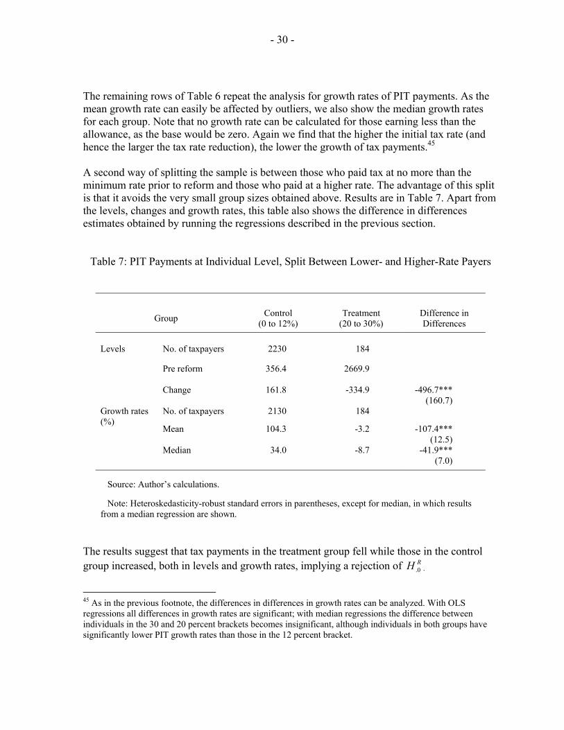
The remaining rows of Table 6 repeat the analysis for growth rates of PIT payments. As the mean growth rate can easily be affected by outliers, we also show the median growth rates for each group. Note that no growth rate can be calculated for those earning less than the allowance, as the base would be zero. Again we find that the higher the initial tax rate (and hence the larger the tax rate reduction), the lower the growth of tax payments.45 A second way of splitting the sample is between those who paid tax at no more than the minimum rate prior to reform and those who paid at a higher rate. The advantage of this split is that it avoids the very small group sizes obtained above. Results are in Table 7. Apart from the levels, changes and growth rates, this table also shows the difference in differences estimates obtained by running the regressions described in the previous section.

Table 7: PIT Payments at Individual Level, Split Between Lower- and Higher-Rate Payers

Group Control (0 to 12%)

Treatment (20 to 30%)

Difference in Differences

Levels No. of taxpayers 2230 184

Pre reform 356.4 2669.9

Change 161.8 -334.9 -496.7*** (160.7)

No. of taxpayers 2130 184 Growth rates (%)

Mean 104.3 -3.2 -107.4*** (12.5)

Median 34.0 -8.7 -41.9*** (7.0)

Source: Author’s calculations. Note: Heteroskedasticity-robust standard errors in parentheses, except for median, in which results from a median regression are shown.

The results suggest that tax payments in the treatment group fell while those in the control group increased, both in levels and growth rates, implying a rejection of RH 0. .

45 As in the previous footnote, the differences in differences in growth rates can be analyzed. With OLS regressions all differences in growth rates are significant; with median regressions the difference between individuals in the 30 and 20 percent brackets becomes insignificant, although individuals in both groups have significantly lower PIT growth rates than those in the 12 percent bracket.

- 31 -

It was stressed in Section III above, however, that if there is no continuum of wage contracts then even some individuals paying tax at the lower rate might have been affected by the reform. To deal with this possibility, we next split the sample by considering a treatment group consisting of all those individuals earning, before the reform, more than 75 percent of the threshold income level at which the higher rates began (which is likely to err on the side of including too many individuals in the treatment group). The results, shown in Table 8, lead to the same conclusion as above: that the reform did not cause the growth of PIT revenues.

Table 8: PIT Payments at Individual Level, Extended Definition of Treatment Group

Control Treatment Difference in Differences

Levels No. of taxpayers 2076 338 Pre reform 306.3 1923.1

Change 156.5 -75.8 -232.3** (104.2)

No. of taxpayers 1976 338 Growth rates (percent) Mean 110.6 8.7 -102.0***

(13.2) Median 35.8 3.0 -32.9***

(5.1) Source: Authors’ calculations. Notes: Heteroskedasticity-robust standard errors in parentheses, except for median, in which results from a median regression are shown. Treatment group defined to include all individuals earning at least 75 percent of the higher-rate threshold.

Turning to the impact of the reform on other variables of interest. Table 9 reports results on payments of PIT and social insurance combined, and for gross incomes, using the same definitions of treatment and control groups as in Table 7 and with a variant of that in Table 8 (including those earning at least half of the higher-rate threshold). For clarity, only the difference in differences estimators are shown, once more both for the levels and for the growth rates. The first and fourth rows show results for PIT payments, and so repeat the results of Table 7 and Table 8. The next row shows results for the sum of PIT and social insurance payments. The next row then shows results for gross income, and the following rows consider the same variables but in growth rates.

- 32 -

Table 9: Difference-in-Differences Estimators for PIT, Total Tax and Gross Income, at Individual-Level

Diff. in Diff., Treatment

Group: 20–30 Percent Diff. in Diff., Extended

Treatment Group Levels Change in PIT -496.7***

(160.7) -232.3** (104.2)

Change in total tax -1860.2*** (452)

-1110.0*** (303.9)

Change in gross income -158.8 (100.9)

-100.9 (67.6)

Growth rates (percent)

Mean growth rate, PIT -107.4*** (125.3)

-102.0*** (13.2)

Mean growth rate, total tax

-51.1*** (3.8)

-47.2*** (3.4)

Mean growth rate, gross income

-41.9*** (3.9)

-41.2*** (3.3)

Median growth rate, PIT -41.9*** (7.0)

-32.9*** (5.1)

Median growth rate, total tax

-28.3*** (4.7)

-24.2*** (3.1)

Median growth rate, gross income

-26.0*** (5.7)

-25.5*** (3.5)

Source: Authors’ calculations. Notes: Heteroskedasticity-robust standard errors in parentheses, except for median, in which results from a median regression are shown. All regressions based on 2,414 individuals. Total tax and PIT show annual figures, while the gross income is a monthly figure. Gross income is gross of PIT and social tax. The extended treatment group is defined to include all individuals earning at least 75 percent of the higher-rate threshold. The results show that it was not only PIT payments that fell in the treatment group relative to the control group, but also the sum of PIT and social insurance payments. Thus RH 0. is also rejected for the sum. So too is the hypothesis that gross income grew more in the treatment groups was higher than in the control group )( 0.

λIH , though not significantly so for the regression in levels. Interestingly, this is in stark contrast to the results for the United States reported in Feldstein (1995), who found that, following the 1986 tax reform, gross incomes increased more, the higher the tax cut. Having found that gross incomes tend to have increased less in the treatment than in the control group, the question is whether this is because the treatment group reduced its labor supply and/or because gross wage rates for these individuals have fallen (in each case relative to the control group). Table 10 reports on this, the results there suggesting that (relative) reductions in both the wage rate and labor supply play a significant role in explaining the relative decline in the gross incomes of the treatment group.

- 33 -

Table 10: Difference in Differences Estimators for Hours Worked and Wage Rate, at Individual-Level

Diff. in Diff., Treatment Group = 20–30 Percent Payers

Diff. in Diff., Extended Treatment Group

Levels Change in hours worked -2.155**

(1.174) -2.135*** (0.811)

Change in wage rate -0.491 (0.564)

-0.280 (0.367)

Growth rates (percent)

Mean growth rate, hours worked

-5.6*** (1.5)

-5.9*** (1.2)

Mean growth rate, wage rate

-37.7*** (5.5)

-38.1*** (4.4)

Median growth rate, hours worked

0 (2.4)

0 (1.8)

Median growth rate, wage rate

-22.4*** (5.4)

-23.4*** (3.8)

Source: Authors’ calculations. Notes: Heteroskedasticity-robust standard errors in parentheses, except for median, in which results from a median regression are shown. All regressions based on 2414 individuals. Total tax and PIT show annual figures, while the gross wage is a monthly figure. The wage rate is gross of PIT and social tax. The extended treatment group is defined to include all individuals earning at least 75 percent of the higher-rate threshold. The thrust of these results is robust to a number of extension, including the use of different definitions of income (including secondary jobs and casual employment), and experimenting with the exclusion of under-employed individuals (working less than 10 hours per week). For brevity, these results are not reported here. All this assumes, however, that survey respondents were fully compliant. The next subsection relaxes this heroic assumption. Allowing for tax evasion and underreporting

In the presence of tax evasion, the allocation of individuals into control and treatment groups is more complicated. One problem is that gross incomes cannot be inferred from reported net incomes, since it is not known how much of that income stems from taxed activities. However, even if gross income data were available, the question would arise of whether an individual whose true income is greater than the higher rate threshold, but who under-declares and so pays tax at the lower rate, should be allocated to the treatment or control group. If such individuals continue not to pay tax after the reform, it may seem that

- 34 -

they were unaffected. In fact though they will be affected, because the cost and benefits of under-declaration have changed. We therefore include them in the treatment group.46 The remaining problem is then how to estimate true gross income. As described above, this can be done using consumption data as a proxy for true total net income, which is less likely to be prone to underreporting in the survey. Indeed we find that consumption, even restricted to non-durable goods, is for many survey families much higher than income. Unlike income, however, consumption data are only available in RLMS at the family level. Individual level consumption data would have enabled the analysis to continue at the individual level, but family level consumption data may be more reliable in that the person providing the information about household consumption will presumably be aware of most major expenditure occurring in the household although not necessarily about the incomes financing the consumption. Formally, for household j comprising individuals I, we thus estimate gross family income as ∑+=

iijj IcI )( λτ .

The use of consumption data provides a further unrelated advantage: consumption is a much better proxy for permanent income than even truthfully reported current income. This is because current income might be affected by temporary shocks. Individuals with a positive (negative) income shock would be wrongly allocated to the treatment (control) group, biasing the results by making a fall in income amongst the treatment group (and a rise in the control group) more likely. To prevent similar effects from the purchase of expensive consumer durables, the consumption variable used here includes only expenditure on non-durables. It is less obvious how to construct treatment and control groups when working at household rather than individual level. The approach here is to take as treatment group those families whose gross family income from employment (that is, gross income estimated as described above, less any pensions or unemployment benefits) per working adult suggests that they would have had one higher rate taxpayer if their incomes had been fully taxed. This, in turn, we take to be the case if gross employment income per working adult is equal to or greater than the threshold at which the higher rate applied prior to reform. Of course, this will exclude some families that would have been subject to the higher rate, since even relatively lower incomes can lead to higher tax rates if they are not equally distributed across working age adults. To check that any differences in results from the previous section are not simply due to moving from individual to household data, Table 11 reports regressions in which the treatment group consists of families that (under the assumption of full compliance) included

46 The point is similar to that which led us to consider individuals close to the threshold as being affected: while such individuals did not face higher tax rates, they are still affected by the tax cut since the costs of avoiding higher tax rates changes.

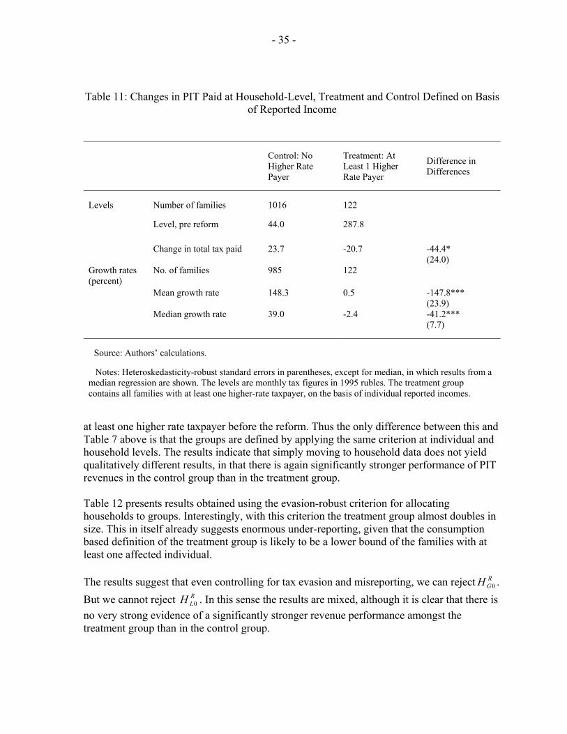
- 35 -

Table 11: Changes in PIT Paid at Household-Level, Treatment and Control Defined on Basis of Reported Income

Control: No Higher Rate Payer

Treatment: At Least 1 Higher Rate Payer

Difference in Differences

Levels Number of families 1016 122

Level, pre reform 44.0 287.8

Change in total tax paid 23.7 -20.7 -44.4* (24.0)

No. of families 985 122 Growth rates (percent)

Mean growth rate 148.3 0.5 -147.8*** (23.9)

Median growth rate 39.0 -2.4 -41.2*** (7.7)

Source: Authors’ calculations. Notes: Heteroskedasticity-robust standard errors in parentheses, except for median, in which results from a median regression are shown. The levels are monthly tax figures in 1995 rubles. The treatment group contains all families with at least one higher-rate taxpayer, on the basis of individual reported incomes.

at least one higher rate taxpayer before the reform. Thus the only difference between this and Table 7 above is that the groups are defined by applying the same criterion at individual and household levels. The results indicate that simply moving to household data does not yield qualitatively different results, in that there is again significantly stronger performance of PIT revenues in the control group than in the treatment group. Table 12 presents results obtained using the evasion-robust criterion for allocating households to groups. Interestingly, with this criterion the treatment group almost doubles in size. This in itself already suggests enormous under-reporting, given that the consumption based definition of the treatment group is likely to be a lower bound of the families with at least one affected individual. The results suggest that even controlling for tax evasion and misreporting, we can reject R

GH 0 . But we cannot reject R

LH 0 . In this sense the results are mixed, although it is clear that there is no very strong evidence of a significantly stronger revenue performance amongst the treatment group than in the control group.

- 36 -

Table 12: Changes in PIT Paid at Household-Level, Treatment and Control Defined by Consumption-Based Estimate of Gross Income

Control Treatment Difference in Differences

Levels Number of families 946 192

Level, pre reform 52.7 156.0

Change in total tax paid 21.7 5.4 -16.3 (19.0)

No. of families 918 189 Growth rates (percent) Mean growth rate 143.4 76.4 -67.0**

(29.8)

Median growth rate 36.7 18.5 -18.3*** (3.7)

Source: Authors’ calculations. Notes: Heteroskedasticity-robust standard errors in parentheses, except for median, in which results from a median regression are shown. Control and treatment group defined using the consumption criterion. Table 13 repeats the analysis for the payment of PIT and social insurance combined, and for gross incomes. The findings for specifications in levels are similar to those in Table 12, in that none of them yields significant differences in levels. For growth rates, however, we find that only for PIT is the difference in differences estimate consistently statistically significant. A key concern in evaluating the 2001 reform is the nature and extent of any impact on compliance. The approach adopted here enables this to be quantified. As reported in Table 14, it implies that prior to the reform individuals in the treatment group declared on average only 52 percent of their incomes, while those in the control group declared 74 percent (which in itself suggests that higher tax rates are associated with lower compliance). Reform leaves compliance amongst the control group virtually unchanged, but for the treatment group it increases by 16 points, to 68 percent. The weighted average growth rate of compliance in the treatment group is thus about one-third. The unweighted average and the median growth rate are very different at 101 percent and 34 percent, suggesting a very skewed distribution. All approaches, however, lead to very high estimates of improvements in compliance in the treatment group. The assumptions underlying these estimates are inevitably quite strong, of course (and especially likely to effect the results in terms of levels). Moreover, it may be that any improvement in compliance was due not to the parametric tax reform but to a synchronous strengthening of tax administration. Nevertheless, the potential magnitude of the improvement in compliance is striking.

- 37 -

Table 13: Difference-in-Differences Estimates for PIT, Total Tax and Declared Income, at Household-Level

Difference in Differences Levels Change in PIT -16.3

(19.0) Change in total tax -63.3

(61.4) Change in declared income -20.9

(167.9) Growth rates (percent)

Mean growth rate, PIT -67.0** (29.8)

Mean growth rate, total tax -10.2 (13.1)

Mean growth rate, declared income -8.5 (11.6)

Median growth rate, PIT -18.3*** (3.7)

Median growth rate, total tax -9.4** (4.0)

Median growth rate, declared income -8.2* (4.6)

Source: Authors’ calculations. Notes: Heteroskedasticity-robust standard errors in parentheses, except for median, in which results from a median regression are shown. Declared income is gross of PIT and social tax. Control and treatment group defined using the consumption criterion.

Table 15 shows that relative gross incomes fell in the treatment group. To establish whether this is due to reduced labor supply or to lower wage rates, Table 16 considers separately gross wages per hour and the number of hours worked, suggesting that the fall in gross income was due only to a lower gross wage rate. Such a fall is precisely what theory predicts, as seen in Section III. Labor supply, for which the theoretical prediction is ambiguous, did not change differentially across groups.

- 38 -

Table 14: Difference-in-Differences Estimates for Compliance, at Household Level

Control Treatment Difference in Differences

Number of families 946 192

Levels Pre reform 73.8 52.0

Change -0.9 16.4 17.3*** (4.4)

Growth rates (%) Mean 22.0 123.3 101.3*** (24.8)

Median 1.1 33.0 34.3*** (5.6)

Source: Authors’ calculations. Notes: Heteroskedasticity-robust standard errors in parentheses, except for median, in which results from a median regression are shown. Control and treatment group defined using the consumption criterion.

Table 15: Difference-in-Differences Estimates for Gross Income, at Household-Level

Control Treatment Difference in Differences

Number of families 946 192

Levels Pre reform 975.0 3124.8

Change 320.6 -556.7 -877.3*** (214.7)

Growth rates (%) Mean 52.2 -2.0 -54.3*** (5.9)

Median 27.4 -13.9 -41.1*** (5.0)

Source: Authors’ calculations. Notes: Heteroskedasticity-robust standard errors in parentheses, except for median, in which results from a median regression are shown. Gross income is gross of PIT and social tax. Control and treatment group defined using the consumption criterion.

- 39 -

Table 16: Difference-in-Differences Estimates for Hours Worked and Wage Rate, Household-Level

Difference in Differences Levels Change in hours worked 1.66

(3.99) Change in wage rate -12.8***

(3.1) Growth rates (%) Mean growth rate, hours worked 4.2

(4.4) Mean growth rate, wage rate -56.8***

(7.6) Median growth rate, hours worked 0

(0.2) Median growth rate, wage rate -38.8***

(7.0) Source: Authors’ calculations. Notes: Heteroskedasticity-robust standard errors in parentheses, except for median, in which results from a median regression are shown. Gross wage rate is gross of PIT and social tax. Control and treatment group defined using the consumption criterion. Summary of results

Whether or not one takes account of tax evasion and misreporting of true incomes in the data, the evidence is that the 2001 reform led to much lower tax revenues from affected individuals—suggesting that the revenue boom which followed was not caused by it. When investigating further the effect on incomes, we find that while the reform reduced gross wage rates, had no measurable effect on labor supply, it strongly boosted compliance.

VII. CONCLUSIONS AND LESSONS

The 2001 Russia flat tax reform has been one of the most influential and widely emulated tax reforms of recent years. Understanding its effects is far from simple, however, given not only the limitations on data—the panel data we use do not include direct observations on tax payments or true gross incomes—but also the wide range of tax and other changes occurring at the same time. In particular, the synchronous substantial reduction in social insurance contributions means that the change in the PIT structure was not the only major change in labor taxation in 2001, so that changes in PIT revenue, and in such other quantities of interest as labor supply and wage rates, cannot be attributed to changes in the PIT alone. Nevertheless, the analysis here does provide some sharp insights into the effect of the PIT reform.

- 40 -

Most important, it is hard to attribute the very strong performance of PIT revenues after the reform to tax reform itself. This conclusion emerges from both the broad macro evidence and, even more strikingly, from the analysis of micro-level data. Evidence of the latter kind is especially compelling in the context of the Russian tax reform, since its structure was such as to have little impact on many individuals and households, so lending itself to a difference in differences analysis comparing developments between a control group of those little affected and a treatment group of those quite strongly affected. And that analysis shows quite robustly that the strongest growth in PIT payments came systematically from those who were little affected by the reform. This is true, for example, whether or not one assumes that survey respondents report their true disposable incomes truthfully, and is robust to a range of empirical strategies. Nor are there any clear signs that the increase in PIT revenue was due to large scale shifting of income from the corporate to personal sectors. There is, in short, no strong evidence that tax reform itself caused the PIT revenue boom. Nor is there any evidence that the rate reduction had any strong incentive effect, with labor supply changes over this period being essentially the same for both those affected and those unaffected. What can be found in the data is a significant reduction in the relative gross wage rates of those most affected by the reform. All this is consistent with, for instance, the elasticity of supply of higher-paid labor being low relative to that of labor demand. This is not to say, however, that the reform did not have significant behavioral effects. For the evidence also points to a marked increase in tax compliance following the reform, with the evidence pointing to an increase of around 16 percentage points in the proportion of their income declared by those affected by the reform. Though the precise estimate should be treated with great caution, there are clear signs of a significant effect. One cannot necessarily attribute this improvement in compliance to the parametric tax reform itself, however. It might reflect the efforts in improved enforcement undertaken by the Russian authorities at around the same time. There is, however, no obvious way of exploring this potential explanation with the data available to us. One could hope to identify effects from any differential changes in enforcement (audit rates and the like) across the regions (enabling a further dimension on differencing), but we have not been able to track down information of this kind. Whatever its cause, however, there is little doubt that a strong improvement in compliance did take place around the time of the flat tax reform, and that this at least mitigated the revenue loss otherwise associated with the parametric reform. What lessons can be drawn for other countries considering the adoption of similar reforms? The purpose here has not been to explain the strong performance of PIT revenues, but only to ask whether this can itself be attributed to the reform. Given that our answer to this question is essentially negative, a key lesson must be that tax-cutting reforms of this kind should not be expected to pay for themselves by greater work effort and improved compliance. Our analysis suggests that the strength of PIT revenues in Russia over this period was largely driven by an increase in real wage rates unrelated to the reform. This may have been associated with the strong energy prices, wider structural reforms, or simply a return to more normal trend levels, and in any event a full understanding is likely to hinge on features of

- 41 -

Russian labor markets. These structural differences may in part account for the difference between the present results for Russia and the finding of strong effects for the United States by Feldstein (1995). Many of those same structural features and rigidities will be present in other transition countries, at least the slowest reformers among them, and so would also be likely to intermediate the effects of similar reforms there. To the extent that the apparent improvement in compliance in Russia was conditioned on the initially high level of noncompliance there, similar effects might be expected, prima facie, in other countries with similar levels of noncompliance. The estimates of the hidden economy47 reported in Table 17 show significant heterogeneity but suggest that Russia has not been atypical. Thus the Russian experience is likely to be relevant for a number of these countries, and the key lesson from the analysis here—whatever the reason for the PIT revenue boom, it lies in something other than behavioral responses to the PIT reform itself—serves an important cautionary note for would-be emulators.

47 Most measures used in transition economies are based on electricity use, the idea being to use differences in the growth rates of electricity usage (as a proxy for the real economy) and reported GDP to deduce size of the shadow economy. There are other methods, however, which are briefly summarised in Eilat and Zinnes (2000) pp. 17-20. All methods, it should be noted, are better suited to identifying changes in the extent of the hidden economy rather than its level.

- 42 -

Table 17. Estimates of the share of the hidden economy in transition countries

Country EZ JKZ Lacko FU Average Russia 33 41 28 35 34 Average of other countries 32 29 27 38 32 Armenia 37 37 Azerbaijan 48 59 33 55 49 Belarus 20 19 31 28 25 Bulgaria 28 33 26 29 Croatia 25 28 26 Czech Republic 19 15 19 18 Estonia 41 19 27 31 29 Georgia 55 63 38 55 53 Hungary 26 29 24 26 Kazakhstan 28 34 28 30 30 Kyrgyz Republic 67 27 59 51 Latvia 26 35 30 25 29 Lithuania 29 25 32 24 28 Macedonia 50 32 41 Moldova 56 38 47 47 Poland 14 14 21 16 Romania 11 18 24 17 Slovakia 12 11 23 15 Slovenia 25 19 22 Tajikistan 52 52 Turkmenistan 11 24.6 18 Ukraine 46 47 35 47.2 44 Uzbekistan 8 8 22 34 18 Notes: The figures give estimates of the share of the shadow economy in total economic activity. The estimates given are the average for 1994/95, except for FU which are the average for 1989-2001. Sources: EZ, JKZ, Lacko: all quoted from Eilat and Zinnes (2000), where EZ are their own estimates, the other two are Johnson, Kaufmann and Zoido-Lobaton (1998) and Lacko (1999). Eilat and Zinnes report the ratio of the shadow to the official economy, which we have converted to a share in the total economic activity. Feige and Urban (2003) report results for different specifications, we quote those estimated with GLS.

- 43 - APPENDIX

DATA

Data sources

Panel data: RLMS GDP deflator: IMF World Economic Outlook.`

RLMS

The individual and household data used in the panel data analysis are from the Russian Longitudinal Monitoring Survey (RLMS) of the Carolina Population Center at the University of North Carolina. The raw data comprise 10,975 (12,121) individuals and 4,006 (4,528) households in the year 2000 (2001). Data are also available for the years 1994 to 1996, 1998, and 2002, but are not used in this paper. The data contain hundreds of variables. Those of interest here are: Individual level data:

pjpayt Average monthly wage over the last 12 months after taxes from primary employer.

wagelm Money received after tax in last 30 days from primary job.

otjwag Money received after tax in last 30 days from secondary job. inciea Money or equivalent from additional employment.

pwrkwh Hours worked in usual week at primary employment. owrkwh Hours worked in usual week at secondary employment.

hrsieapw Hours worked in additional employment during last 30 days. ownent Whether respondent is owner or co-owner of enterprise.

Household level data:

alcohln, breadn, dairyn, eatoutn, eggsn, fatn, fishn, fruitsn, meatn, ofoodn, potaton, sugarn, vegetn

Nominal expenditure on different food items.

fuelaun, clothn, fuelgsn, fuelwdn, paymntn, rentun, servicn, tobacn, assistn, luxurn

Nominal expenditure on different non-food non-durable items.

ncat1 – ncat6 Number of individuals falling into following categories: 1: children <7 yrs; 2: children 7-18 yrs; 3: working age males; 4: working age females, 5: post-work age males; 6; post-work age females.

- 44 - APPENDIX

Calculation of tax payments When calculating tax revenues and pre-tax incomes, care has to be taken to correctly account for the personal allowances individuals are entitled to. This is complicated by the fact that the total yearly allowance depends on the monthly pattern of income receipts. For instance, in the year 2000 an individual received a monthly allowance of 264 rubles until the month in which cumulative yearly income exceeded 20,000 rubles. From that month onwards the allowance was 132 rubles until the cumulative yearly income reached 50,000 rubles, beyond which there was no further entitlement to an allowance. In order to be able to calculate the yearly allowance, an assumption needs to be made about the distribution of wage payments over the year. We assume that the same nominal wage is paid evenly throughout the year, although in theory there was an incentive to postpone payments to later months, to benefit as long as possible from the allowances. This incentive is unlikely to be strong, however, given the low level of the allowance. Any additional allowances, such as those linked to dependents or incapacity, are ignored. Having obtained an estimate of the allowance, the remaining calculations are straightforward applications of the published tax rates and thresholds. As taxes are assessed at the individual level, there is no further difficulty in calculating taxes at the household level, which are just the sum of individual taxes. Cleaning Individual data The raw data consist of 23,096 observations, 10,975 from 2000 and 12,121 from 2001. The following table shows how many observations are lost due to cleaning for each of a list of criteria. Note that the total number of lost observations is smaller than the sum for each individual criterion, because individuals can fulfill more than one of the criteria. Dropping individuals who own their own business, for example, only leads to the additional loss of 17 individuals in 2000, once the previous criteria have been applied. Statistics reported in the paper are based on the data cleaned only on the criteria in the upper half of the table (7,913 observations). The regressions are generally based on the balanced panel with the “pjpayt” variable present (4,828 observations or 2,414 individuals). Household data The raw data consist of 8,534 observations, 4,006 from 2000 and 4,528 from 2001. The following table reports the numbers of observation lost due to cleaning.

- 45 - APPENDIX

Table 18: Cleaning of Individual-Level Data

Criterion Observations Dropped (Remaining)

Keep if between 20 and 60 years of age throughout 2000 to 2001 10400 Drop if do not report how many hours they work or claim to work more than 84 hours per week

4516

Drop if do not report any income from primary employment 14131 Drop if own their own business 63 All of the above 15183 (7913) Additionally

keep if report “wagelm” (necessary for Table 5) 1117 (6796) keep if report “pjpayt” 704 (7209) keep if present in both 2000 and 2001 2437 (5476) keep if present in both 2000 and 2001 and report “wagelm” 3637 (4276) keep if present in both 2000 and 2001 and report “pjpayt” (basis for

regressions from Table 6 onwards) 3085 (4828)

Source: Authors’ calculations.

Table 19: Cleaning of Household-Level Data

Criterion Observations Dropped (Remaining)

Keep if can be matched to individual data, in case of family split keep larger part of a family

1267 (7267)

Additionally keep if at least one working-age adult in household 1860 (5407) keep if report “pjpayt” for at least one member of household 2771 (4496) both of the above 2989 (4278) Additionally keep if households present in 2000 and 2001 and the household composition

does not change 2002 (2776)

Source: Authors’ calculations.

- 46 -

REFERENCES

Allingham, Michael, and Agnar Sandmo, 1972, “Income Tax Evasion: A Theoretical Analysis,” Journal of Public Economics, Vol. 1, pp. 323–38.

Andreoni, James, Brian Erard, and Jonathan Feinstein, 1999, “Tax Compliance,” Journal of

Economic Literature, Vol. 36, pp. 818–60. Blundell, R., A. Duncan, and C. Meghir, 1998, “Estimating Labor Supply Responses Using

Tax Reforms,” Econometrica, Vol., 66, pp. 827–62. Chua, Dale, 2003, “Tax Reform in Russia,” in Russia Rebounds, ed. by David Owen and

David Robinson (Washington: International Monetary Fund). Eissa, N., 1995, “Taxation and Labor Supply of Married Women: The Tax Reform Act of

1986 As a Natural Experiment,” NBER Working Paper No. 5023 (Cambridge, Massachusetts: NBER).

Eilat, Y., and C. Zinnes, 2000, “The Evolution of the Shadow Economy in Transition

Countries: Consequences for Economic Growth and Donor Assistance,” CAER II Discussion Paper No. 83 (Cambridge, Massachusetts: Harvard Institute for International Development).

Engel, Eduardo E., and James R. Hines, Jr., 1999, “Understanding Tax Evasion Dynamics,”

NBER Working Paper 6903 (Cambridge, Massachusetts: NBER). Feige, E.L., and I. Urban, 2003, “Estimating the Size and Growth of Unrecorded Economic

Activity in Transition Countries: A Reevaluation of Electric Consumption Method Estimates and Their Implications,” William Davidson Institute Working Paper 636.

Feldstein, M., 1995, “The Effect of Marginal Tax Rates on Taxable Income: A Panel Study

of the 1986 Tax Reform Act,” Journal of Political Economy, Vol. 103, pp. 551–72. Friedman, Eric, Simon Johnson, Daniel Kaufman, and Pablo Zoido-Lobaton, 2000, “Dodging

the Grabbing Hand: The Determinants of Unofficial Activity in 69 Countries,” Journal of Public Economics, Vol. 76, pp.459–93.

Glavatskaya, N., and K. Seryanova, eds., 2003, “Tax Reform in Russia: Problems and

Solutions,” Institute for Economies in Transition Working Paper No. 67. (In Russian; available at http://www.iet.ru/papers/67/.)

Gordon, Roger, and Jeffrey Mackie-Mason, 1994, “Tax Distortions to the Choice of

Organizational Form,” Journal of Public Economics, Vol. 55, pp. 297–306.

- 47 -

Gordon, Roger, and Joel Slemrod, 1998, “Are ‘Real’ Responses to Taxes Simply Income Shifting Between Corporate and Personal Tax Bases?” NBER Working Paper 6576 (Cambridge, Massachusetts: NBER).

Hall, Robert E., and Alvin Rabushka, 1995, The Flat Tax, 2nd edition (Stanford: Hoover

Institution Press). International Monetary Fund, 2000, “Russian Federation: Selected Issues and Statistical

Appendix” (Country Report 02/75), April 2002. Johnson, S., D. Kaufmann, and P. Zoido-Lobaton, 1998, “Regulatory Discretion and the

Unofficial Economy,” American Economic Review, Vol. 88 (2), pp. 387–432. Konings, Jozef, and Hartmut Lehmann, 2002, “Marshall and Labor Demand in Russia: Going

Back to Basics,” Journal of Comparative Economics, Vol. 30, pp.134–59. Kwon, Gohoon, 2003, “Post-Crisis Fiscal Revenue Developments in Russia: From an Oil

Perspective,” Public Finance and Management, Vol. 3, pp. 503–30. Lacko, M., 1996, “Hidden Economy—An Unknown Quantity? Comparative Analysis of

Hidden Economies in Transition Countries in 1989–1995, Working Paper No. 9905 (University of Linz: Department of Economics).

Rabushka, Alvin, 2003, “The Flat Tax in Russia and the New Europe,” Brief No. 2003

(Washington: National Center for Policy Analysis). RLMS, 2004, “Russian Longitudinal Monitoring Survey” (Carolina Population Center:

University of North Carolina). Schneider, Friedrich, and Dominik Enste, 2000, “Shadow Economies: Sizes, Causes, and

Consequences,” Journal of Economic Literature, Vol. 38, pp. 77–114. Sinelnikov-Mourylev, S. S. Batkibekov, P. Kadochnikov, and D. Nekipelov, 2003,

“Evaluation of the Results of Personal Income Tax Reform in Russian Federation” (Institute for Economies in Transition Working Paper), at http://www.iet.ru/papers/52/index.htm

Slemrod, Joel, 2001, “A General Model of the Behavioral Response to Taxation,”

International Tax and Public Finance, Vol. 8, pp.119–28. Slemrod, Joel, and Schlomo Yitzhaki, 2002, “Tax Avoidance, Evasion, and Administration,”

in Handbook of Public Economics, ed. by Alan Auerbach and Martin Feldstein (North-Holland: Amsterdam) pp. 1423–70.

Yitzhaki, Schlomo, 1974, “A Note on ‘Income Tax Evasion: A Theoretical Analysis’,”

Journal of Public Economics, Vol. 3, pp. 201–02.