anisotropic-ray-theory geodesic deviation and two...

Anisotropic-ray-theory geodesic deviationand two-point ray tracingthrough a split intersection singularity

Petr Bulant & Ludek Klimes

Department of Geophysics, Faculty of Mathematics and Physics, Charles University inPrague, Ke Karlovu 3, 121 16 Praha 2, Czech Republic,http://sw3d.cz/staff/bulant.htm, http://sw3d.cz/staff/klimes.htm

Summary

We demonstrate the principal problems with tracing the anisotropic–ray–theory S–waverays. While the initial–value rays can safely be traced by solving Hamilton’s equationsof rays, it is often impossible to determine the coefficients of the equations of geodesicdeviation (paraxial ray equations, dynamic ray tracing equations) and to solve themnumerically. As the result, we often know neither the matrix of geometrical spreadingnor the phase shift due to caustics. We show how surprisingly large is the number ofrays which cannot be correctly calculated in the velocity model with a split intersectionsingularity.

Keywords

Wave propagation, elastic anisotropy, heterogeneous media, anisotropic ray theory,geodesic deviation, KMAH index, two–point ray tracing, S–wave singularities.

1. Introduction

In a generally anisotropic medium, the S–wave slowness sheets of the slowness surfaceare usually mostly separated and intersect in at up to 32 point S–wave singularities(Vavrycuk, 2005a; 2005b). In this case, outside the point singularities, the anisotropic–ray–theory rays stay at the faster or slower S–wave slowness sheet, respectively. Whenapproaching the point singularities, the limiting case again corresponds to staying at thefaster or slower S–wave slowness sheet, respectively. In a generally anisotropic medium,we thus have to separate the slowness surface into the P–wave slowness sheet, the fasterS–wave slowness sheet and the slower S–wave slowness sheet.

However, in a transversely isotropic medium, the S–wave slowness sheets mayintersect along intersection singularities (Vavrycuk, 2003). If a medium is close totransversely isotropic but is not transversely isotropic, the intersection singularity issplit, the slower S–wave slowness sheet separates from the faster S–wave slowness sheet,forming smooth but very sharp edges on both sheets.

When the slowness vector of a ray smoothly pass through a split intersectionsingularity or close to the vicinity of a conical or wedge singularity, the ray–velocityvector rapidly changes its direction and creates a sharp bend on the ray. This sharpbend is connected with a rapid rotation of the eigenvectors of the Christoffel matrix.The sharply bent rays thus cannot describe the correct wave propagation and indicatea failure of ray methods.

Seismic Waves in Complex 3–D Structures, 24 (2014), 179–187 (ISSN 2336–3827, online at http://sw3d.cz)

179

The sharply bent rays can safely be traced by solving Hamilton’s equations of rays.On the other hand, the dependence of the second derivatives of the Hamiltonian functionwith respect to the slowness vector along the ray contains a narrow spike resemblinga Dirac distribution. This narrow spike destroys the numerical integration of theequations of geodesic deviation (paraxial ray equations, dynamic ray tracing equations),and the matrix of geometrical spreading becomes random behind the spike. Moreoverthe numerical integration can generate several spurious changes of the signature of thematrix of geometrical spreading, which may result in various incorrectly large KMAHindices. Random incorrect KMAH indices cannot be used for the determination of rayhistories during two–point ray tracing. Even if we removed the KMAH index from rayhistories, we could not use the randomly generated matrix of geometrical spreading fortwo–point ray tracing.

In this paper, we numerically demonstrate the problems with two–point ray tracingin velocity model SC1 II which contains a split intersection singularity.

2. Velocity model SC1 II

At the depth of 0 km, velocity model SC1 II is transversely isotropic with the tilted axisof symmetry. At this depth, the slowness surface contains an intersection singularity.At the depth of 1.5 km, velocity model SC1 II is very close to isotropic, but is slightlycubic and its symmetry axes coincide with the coordinate axes. This means that, at alldepths except 0 km, velocity model SC1 II is very close to transversely isotropic, but isslightly tetragonal. Whereas the transversely isotropic medium contains the intersectionsingularity through which the rays pass without rotation of the eigenvectors of theChristoffel matrix (Vavrycuk, 2001, sec. 4.3), in the slightly tetragonal medium, theS–wave slowness surface is split at this unstable singularity (Crampin, 1981) and theeigenvectors of the Christoffel matrix rapidly rotate by 90◦ there.

3. Initial–value tracing of anisotropic–ray–theory S–wave rays

Previous versions of the SW3D software package CRT were designed to trace theanisotropic–ray–theory P–wave rays and the anisotropic common S–wave rays using theaverage S–wave Hamiltonian function according to Klimes (2006). We did not consideranisotropic–ray–theory S–wave rays for obvious problems with S–wave slowness surfacesingularities. Now we have added an optional possibility to calculate anisotropic–ray–theory S–wave rays to the package CRT version 7.10 (Bucha & Bulant, 2014) for testingpurposes.

Optional tracing of anisotropic–ray–theory S–wave rays is designed for generalanisotropy with point S–wave singularities only. We thus a priori choose the fasterS wave or the slower S wave. In each step of anisotropic–ray–theory S–wave ray tracing,the Christoffel matrix is calculated together with its eigenvalues and correspondingeigenvectors. We then select the a priori given anisotropic–ray–theory S wave (theslower one or the faster one) for the calculation of the ray.

The rays of the selected anisotropic–ray–theory S wave can safely be traced bysolving Hamilton’s equations of rays. Unfortunately, the equations of geodesic de-viation (paraxial ray equations, dynamic ray tracing equations) contain the second–order derivatives of the Hamiltonian function with respect to the slowness vector.Expressions for these derivatives contain the difference of the S–wave eigenvalues of

180

the Christoffel matrix in the denominator. If the difference of the S–wave eigenvalues ofthe Christoffel matrix is smaller than the rounding error, the second–order derivativesof the Hamiltonian function with respect to the slowness vector become random and,in consequence, the matrix of geometrical spreading becomes random, too. If we wishthe rays with a reasonably defined matrix of geometrical spreading and a reasonablydefined phase shift due to caustics, we have to terminate tracing of a ray if the relativedifference between the S-wave eigenvalues of the Christoffel matrix is smaller then theprescribed limit which we named DSWAVE. The maximum angular numerical error of theeigenvectors of the Christoffel matrix in radians is then roughly equal to the ratio ofthe relative rounding error to parameter DSWAVE.

4. Problems of two–point rays tracing in velocity model SC1 II

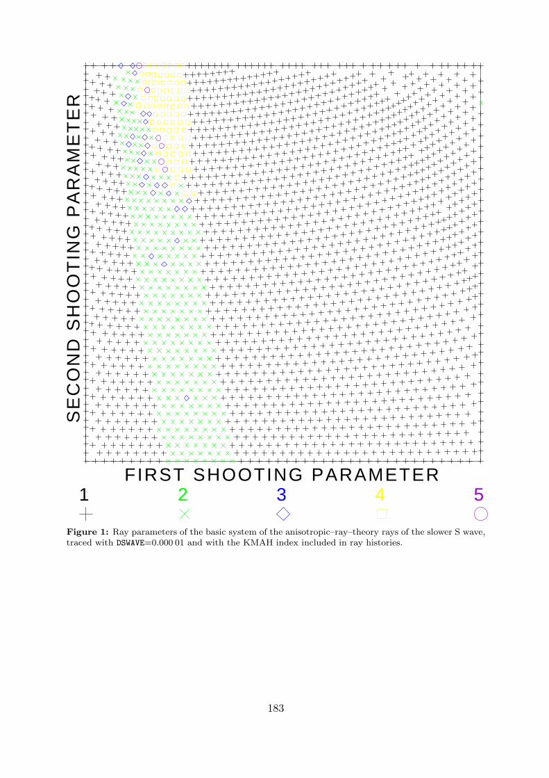
We chose the value 0.000 01 of the above mentioned parameter DSWAVE and traced theinitial–value rays of the slower S wave. The ray parameters of the rays are displayed inFigure 1. The black plus crosses (ray history 1) correspond to the rays which do nottouch a caustic and thus have the KMAH index of 0. The belt of other symbols roughlycorresponds to the sharply bent rays (Klimes & Bulant, 2014, fig. 3) which should havethe KMAH index of 1. The yellow squares (ray history 4) indeed correspond to rayswith the KMAH index of 1. We see that the boundary between the KMAH index of0 and the KMAH index of 1 is not smooth, which means that the value of the KMAHindex is sometimes incorrect for the chosen value of parameter DSWAVE. We also observeviolet circles (ray history 5) corresponding to the rays with the incorrect value 2 of theKMAH index. The value 0.000 01 of parameter DSWAVE is thus too small for the correctdetermination of the matrix of geometrical spreading and of the KMAH index. Onthe other hand, green times crosses (ray history 2, KMAH=0) and blue diamonds (rayhistory 3, KMAH=1) correspond to the rays whose tracing has been terminated dueto the relative difference of the S–wave eigenvalues smaller than DSWAVE=0.000 01. Therays whose tracing has been terminated completely cover the region of the two–pointrays corresponding to the reverse branch of the wavefront triplication, refer to Figures3 and 5, and to Klimes & Bulant (2014, figs. 3, 4). If we wish to obtain these two–pointrays, we have to considerably decrease the value of parameter DSWAVE, although weknow, that the matrix of geometrical spreading and the KMAH index will then becomerandom.

We thus chose the value 0.000 000 000 01 of parameter DSWAVE and traced the initial–value rays of the slower S wave. The ray parameters of the rays are displayed in Figure 2.The only ray whose tracing has been terminated corresponds to the violet circle (rayhistory 5). All other initial–value rays have been calculated, but with random values ofthe KMAH index. The random values of the KMAH index are 0 (ray history 1), 1 (rayhistory 2), 2 (ray history 3) and 4 (ray history 4).

During two–point ray tracing according to Bulant (1996; 1999), we have to deter-mine the boundaries between the regions of different ray histories, in this case betweenthe regions of different KMAH indices. Determination of the boundaries between theregions of random KMAH indices of Figure 2, using additional auxiliary rays with againrandom KMAH indices, obviously represents a disaster for the two–point ray tracingalgorithm. The ray parameters of all anisotropic–ray–theory rays of the slower S wavetraced with DSWAVE=0.000 000 000 01 during the two–point ray tracing are displayed inFigure 3 together with the triangulation of the ray–parameter domain. The random

181

values of the KMAH index are 0 (ray history 1), 1 (ray history 2), 2 (ray history 3),3 (ray history 5), 4 (ray history 4), 5 (ray history 9), 6 (ray history 7) and 10 (rayhistory 8). Ray history 6 corresponds to the ray whose tracing has been terminated.The large red plus crosses correspond to the rays approximately leading to the receivers.The receivers are located in a vertical well at a distance of 1 km from the source. Thereceivers extend from the depth of 1.32 km below the source to the elevation of 0.48 kmabove the source with spacing of 0.04 km (Klimes & Bulant, 2014, fig. 3).

In order to trace the anisotropic–ray–theory rays of the slower S wave in velocitymodel SC1 II, we have optionally removed the KMAH index from ray histories. Theray parameters of the initial–value rays traced with DSWAVE=0.000 000 000 01 and withthe KMAH index removed from ray histories are displayed in Figure 4. In this case, theonly ray whose tracing has been terminated corresponds to the green times cross (rayhistory 2). All other rays have been calculated and have equal ray history 1. In thisway, we can find the rays approximately leading to the receivers, see Figure 5. For thepictures of ray trajectories and wavefronts refer to Klimes & Bulant (2014, figs. 3, 4).

Acknowledgements

The research has been supported by the Grant Agency of the Czech Republic under con-tract P210/10/0736, by the Ministry of Education of the Czech Republic within researchprojects MSM0021620860 and CzechGeo/EPOS LM2010008, and by the members of theconsortium “Seismic Waves in Complex 3–D Structures” (see “http://sw3d.cz”).

References

Bucha, V. & Bulant, P. (eds.) (2014): SW3D–CD–18 (DVD–ROM). Seismic Waves inComplex 3–D Structures, 23, 211–212, online at “http://sw3d.cz”.

Bulant, P. (1996): Two–point ray tracing in 3-D. Pure appl. Geophys., 148, 421–447.Bulant, P. (1999): Two–point ray–tracing and controlled initial–value ray–tracing in

3-D heterogeneous block structures. J. seism. Explor., 8, 57–75.Crampin, S. (1981): A review of wave motion in anisotropic and cracked elastic–media.

Wave Motion, 3, 343–391.Klimes, L. (2006): Common–ray tracing and dynamic ray tracing for S waves in a

smooth elastic anisotropic medium. Stud. geophys. geod., 50, 449–461.Klimes, L. & Bulant, P. (2014): Anisotropic–ray–theory rays in velocity model SC1 II

with a split intersection singularity. Seismic Waves in Complex 3–D Structures,24, 189–205, online at “http://sw3d.cz”.

Vavrycuk, V. (2001): Ray tracing in anisotropic media with singularities. Geophys. J.int., 145, 265–276.

Vavrycuk, V. (2003): Generation of triplications in transversely isotropic media. Phys.Rev. B, 68, 054107-1–054107-8.

Vavrycuk, V. (2005a): Acoustic axes in weak triclinic anisotropy. Geophys. J. int., 163,629–638.

Vavrycuk, V. (2005b): Acoustic axes in triclinic anisotropy. J. acoust. Soc. Am., 118,647–653.

182

FIRST SHOOTING PARAMETER

SE

CO

ND

SH

OO

TIN

G P

AR

AM

ET

ER

1 2 3 4 5

Figure 1: Ray parameters of the basic system of the anisotropic–ray–theory rays of the slower S wave,

traced with DSWAVE=0.000 01 and with the KMAH index included in ray histories.

183


SE

CO

ND

SH

OO

TIN

G P

AR

AM

ET

ER

1 2 3 4 5


traced with DSWAVE=0.000 000 000 01 and with the KMAH index included in ray histories.

184


SE

CO

ND

SH

OO

TIN

G P

AR

AM

ET

ER

1 2 3 4 5 6 7 8 9

Figure 3: Ray parameters of all traced anisotropic–ray–theory rays of the slower S wave, including the

triangulation of the ray–parameter domain. The rays are traced with DSWAVE=0.000 000 000 01 and with

the KMAH index included in ray histories. The large red crosses correspond to the rays approximately

leading to the receivers.

185


SE

CO

ND

SH

OO

TIN

G P

AR

AM

ET

ER

1 2


traced with DSWAVE=0.000 000 000 01 and with the KMAH index removed from ray histories.

186


SE

CO

ND

SH

OO

TIN

G P

AR

AM

ET

ER

Figure 5: Ray parameters of all traced anisotropic–ray–theory rays of the slower S wave, including

the triangulation of the ray–parameter domain. The rays are traced with DSWAVE=0.000 000 000 01

and with the KMAH index removed from ray histories. The large red crosses correspond to the rays

approximately leading to the receivers. It is obvious from the distribution of auxiliary rays shot towards

the receivers that the paraxial approximation inevitably failed in the belt of sharply bent rays. The

isolated cluster of auxiliary rays corresponds to the ray which could not be traced, refer to the green

times cross in Figure 4.

187

anisotropic-ray-theory geodesic deviation and two...

Documents