Geodesic Deviation and Weak-Field Solutions

Luciano Rezzolla∗

SISSA, International School for Advanced Studies and INFN, Trieste, Italy

Department of Physics and Astronomy, Louisiana State University, Baton Rouge, LA 70803 USA

Lectures given at the:

3rd VIRGO-EGO-SIGRAV School on Gravitational Waves

May 24th - 28th , 2004 Cascina (PI), Italy

∗www.sissa.it/∼rezzolla

1

A note on conventions

I here use a spacelike signature (−, +, +, +) and a system of units in which c = 1. Greek

indices are taken to run from 0 to 3, Latin indices from 1 to 3, and we adopt the standard

convention for the summation over repeated indices. Furthermore we will indicate three-

vectors with an arrow (e.g. ~U ), four-vectors with bold symbols or Greek letters (e.g. U or

ξ), and tensors with slanted bold symbols (e.g. T ).

1 Geodesic deviation equation

1.1 Geodesic Equation

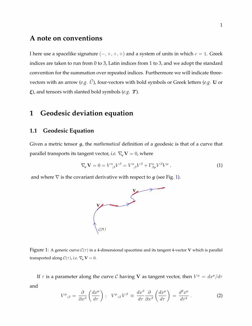
Given a metric tensor g , the mathematical definition of a geodesic is that of a curve that

parallel transports its tangent vector, i.e. ∇VV = 0, where

∇VV = 0 = V α

;βV β = V α,βV β + Γα

βµVβV µ , (1)

and where ∇ is the covariant derivative with respect to g (see Fig. 1).

V

V

C( )τ

Figure 1: A generic curve C(τ) in a 4-dimensional spacetime and its tangent 4-vector V which is parallel

transported along C(τ), i.e. ∇VV = 0.

If τ is a parameter along the curve C having V as tangent vector, then V µ = dxµ/dτ

and

V µ,β =∂

∂xβ

(dxµ

dτ

); V µ,β V β ≡ dxβ

dτ

∂

∂xβ

(dxµ

dτ

)=

d2xµ

dτ 2. (2)

2

so that the geodesic equation (1) can be written as a second-order differential equation

d2xµ

dτ 2+ Γµ

αβ

dxα

dτ

dxβ

dτ= 0 , (3)

having xµ(P0) and dxµ/dτ(P0) as initial conditions. If the particle has a nonzero mass, τ

can then be associated to the proper time measured by the particle along C.

On the other hand, a physical definition of a geodesic is that of a curve along which

a freely falling particle moves. Note that the sense of “geodetic-deviation” is not that

of a deviation from a purely geodetic motion resulting from the application of a force.

Rather, the concept of geodetic deviation follows from the comparison between two ad-

jacent geodesics and measures how and when their separation varies. In this Section in

particular, we will show how the deviation from a geodesic motion (meant as the evolu-

tion of the separation measured between two adjacent geodesics) can indeed be related

to a nonzero curvature of the spacetime, or, to use a Newtonian language, to the presence

of tidal force.

However, before we consider the concept of geodesic deviation in full General Rela-

tivity, it is instructive to first look at this problem in Newtonian gravity, where the basic

features are also present.

1.2 Geodesic deviation in Newtonian gravity

For this, let us consider the Newtonian gravitational potential

Φ = Φ(xa) , (4)

and two curves C1 and C2 of parameter t (e.g. the coordinate time) describing the motion

of two test particles P and Q in the gravitational potential Φ. At any given time t the two

particles will have positions xa and za which will clearly vary in time. Furthermore, let

ηa(t) be the components of the 3-vector separating the two particles at any time, i.e. (see

Fig. 2)

za = za(t) = xa(t) + ηa(t) . (5)

3

aη

az

xa

P0

PQ

C C1 2

Q0

Figure 2: Trajectories of two freely falling particles in a gravitational potential Φ. The 3-vector ~η measures

the distance between the two particles at any time.

Because there is only one force applied (the gravitational one), the equations of motion

will be particularly simple and have the form

xa(t) = −(∂aΦ)P , (6)

za(t) = −(∂aΦ)Q = xa(t) + ηa(t) , (7)

where xa ≡ d2xa/dt2 and (∂aΦ)P,Q are the gravitational forces at time t acting on P and Q,

respectively. We can now expand in a Taylor series the gravitational field Φ in Q in terms

of the separating 3-vector ηa, i.e.

(Φ)Q = (Φ)P + ηb(∂bΦ)P +O(ηaηa) , (8)

so that equations (6) and (7) can be written as

za = xa + ηa = −(∂aΦ)Q = −∂a[(Φ)P + ηb(∂bΦ)P ] = −(∂aΦ)P − ηb(∂a∂bΦ)P , (9)

or equivalently

ηa = −(∂a∂bΦ)ηb = −Kabη

b . (10)

where Kab ≡ ∂a∂bΦ.

Equation (10) represents the geodesic deviation equation in Newtonian physics and ex-

presses the fact that the distance between the two freely falling particles will vary if they

4

move in a gravitational field that is nonuniform. Furthermore, since ηa = 0 at all times if

Kab = 0 at all times, equation (10) underlines how, in principle, the relative acceleration

between the two particles cannot distinguish between a uniform gravitational field (i.e.

∂aΦ = 0) and a zero one (i.e. Φ = 0). Of course, we know from astronomical observations

that in Newtonian gravity Φ ∼ 1/r and so Kab ∼ 0 only at large distances from the source

of Φ, where Φ ∼ 0.

In the following Section we will see that many of the considerations made here con-

tinue to hold true also in General Relativity.

5

1.3 Geodesic deviation in General Relativity

With the insight gained in Newtonian gravity, we can now consider the problem of geode-

tic deviation in General Relativity. It has been shown that the differences that emerge

when a 4-vector V is parallel transported along a loop along two different routes is di-

rectly related to the curvature tensor of the spacetime in which the loop lies. Using an

index notation, this is expressed by the equation

2∇[α∇β]Vµ = Rµ

ναβV ν , (11)

where

2∇[α∇β]Vµ = ∇αβV µ −∇βαV µ = V µ

;αβ − V µ;βα , (12)

and R is the Riemann (or curvature) tensor defined as

Rµνβα ≡ Γµ

να,β − Γµνβ,α + Γµ

σβΓσνα − Γµ

σαΓσνβ . (13)

Note that because the Christoffel symbols are linear combinations of the first-order partial

derivatives of the metric, the Riemann tensor R (13) is effectively a combination of first

and second-order partial derivatives of the metric.

Equation (11) is important for a number of different reasons. Firstly it shows that, in

general, in a curved spacetime the covariant derivatives do not commute. Secondly it

expresses a relation between a “failed parallel transport” (i.e. ∇[α∇β]Vµ 6= 0) and the local

curvature, i.e.

(deviation from parallel transport) ! (curvature) . (14)

On the other hand, we have also seen the relation between parallel transport and geodesic

motion, i.e.

(parallel transport) ! (geodesic motion) , (15)

and it would not be surprising, therefore, to find out that there is a close logical connection

between the deviation from a geodesic in the presence of curvature, i.e.

(deviation from parallelism in geodesic motion) ! (curvature) . (16)

6

This is what we will show in a rigorous way.

Consider therefore a congruence of geodesic curves of parameter τ and tangent vector

V, where

V α ≡ dxα

dτ, and ∇

VV = 0 . (17)

ν1

C C1 2

V

ξ

ν2

ν3

ν4

ν5

Figure 3: Congruence of geodesic curves of parameter τ and tangent vector V, where each geodesic is

distinguished by the value of a parameter ν so that the 4-vector ξ represents the separation vector.

Each geodesic is distinguished by the value of a parameter ν so that the separation vector

ξ between two adjacent geodesics is given by

ξα ≡ dxα

dν. (18)

It is now not difficult to show that the commutator between V and ξ is given by

[V, ξ]α ≡ V β∂βξα − ξβ∂βV α =

=

(dxβ

dτ

∂

∂xβ

)ξα −

(dxβ

dν

∂

∂xβ

)V α =

=d2xα

dτdν− d2xα

dνdτ= 0 , (19)

from which we can deduce that the Lie derivative of ξ along V is also zero, i.e.

LVξ ≡ [V, ξ] = 0 . (20)

7

A more extended discussion of the Lie derivatives and of its properties is presented in the

Appendix 1.4.

We can now use the result (20) to show that

LVξβ = V α∂αξβ − ξα∂αV β =

= ξβ,αV α − V β

,αξα =

= ξβ;αV α − V β

;αξα =

= ∇Vξβ −∇ξV

β = 0 , (21)

where we have used the property that in taking the Lie derivative of a contravariant

vector the partial derivatives can be replaced by the covariant derivatives1.

Stated it differently, expression (21) shows that the parallel transport of ξ along V is

equivalent to the parallel transport of V along ξ, i.e.

∇Vξ = ∇ξV .

Recalling that we are interested in finding out about the geodesic deviation through

the second-order covariant derivative, we can now use (1.3) to calculate the double co-

variant derivative of ξ along V, which turns out to be

∇V(∇

Vξ) = ∇

V(∇ξV) . (23)

At this point it is quite easy to appreciate the similarities between the left-hand-side

of expression (23) and the corresponding lef-thand-side of the Newtonian equation (10).

In particular, the following association is quite natural

ηa : (separation of particles′ trajectories) ! ξα : (separation of geodesics) , (24)

1This property is rooted in the symmetry of the lower indices of the Christoffel symbols Γαβµ, i.e.

LV

ξα = ξα;βV β − V α

;βξβ = ξα,βV β − ξα

,βV β + Γαβµ

[V βξµ − V µξβ

]= ξα

,βV β − ξα,βV β . (22)

8

as well as

t : (parameter along the particles′ trajectories) ! τ : (parameter along the geodesics) ,

(25)

from which it follows that

ηa ! ∇V∇

Vξα =

D2

Dτ 2ξα , (26)

where we have introduced the symbol D/Dxα to indicate the covariant derivative along

xα and D/Dτ as a shorthand for the directional covariant derivative along the tangent

vector V, i.e.

;α =D

Dxα, (27)

∇V

= V α D

Dxα=

dxα

dτ

D

Dxα=

D

Dτ, (28)

so thatD2ξα

Dτ 2≡ d2ξα

dτ 2+ Γα

µν

dξµ

dτ

dξν

dτ. (29)

At this point we need to quantify ∇V∇

Vξα and fortunately this is rather easy if one

uses the following identity (prove it!)2

2∇[X∇

Y]Zα −∇

[X,Y]Zα = ∇

X(∇

YZα)−∇

Y(∇

XZα)−∇[X,Y]Z

α = RαβµνZ

βXµY ν . (32)

where X, Y are generic 4-vectors.

If we now take X = Z = V and Y = ξ, then ∇[V,ξ]Vα = 0 (i.e. V and ξ commute) and

expression (32) simplifies into

2∇[V∇ξ]Vα = Rα

βµνVβV µξν , (33)

2In your proof bear in mind that

2∇[X∇Y]Zα = ∇

X(∇

YZα)−∇

Y(∇

XZα) , (30)

and that

∇[X,Y]Zα = Xµ(∇µY ν)(∇νZα)− Y µ(∇µXν)(∇νZα) . (31)

9

Exploiting now the fact that∇VV α = 0 (V is the tangent vector of a geodesic curve) and

∇V∇ξV = ∇

V∇

Vξ [i.e. equation (23)], the left-hand-side of equation (33) can be written

explicitely as

∇V∇ξV

α −∇ξ∇VV α = ∇

V∇ξV

α = ∇V∇

Vξα. (34)

thus finally leading to the expression for the equation of geodesic deviation

∇V∇

Vξα = Rα

βµνVβV µξν . (35)

This tells us about the “forces” acting on an object, i.e. how geodesics change their dis-

tance as they whirl in spacetime.

Recalling expression (27) for the directional covariant derivative along the tangent

vector V, then equation (35) can be also written as

D2ξα

Dτ 2= −Kα

µξµ , (36)

where we have exploited the antisymmetry on the last two indices of the Riemann tensor3

to rewrite (35) as

∇V∇

Vξα = −Rα

βνµVβξνV µ = −Rα

βµνVβξµV ν , (39)

and where we have defined

Kαµ ≡ Rα

βµνVβV ν . (40)

The analogies between the Newtonian expression for the variation of the freely falling

particles (10) and the general relativistic expression for the geodesic deviation (36) is par-

ticularly apparent when we compare side-by-side the two expressions, i.e

d2ηα

dt2= −Ka

bηb ,

D2ξα

Dτ 2= −Kα

βξβ . (41)

(Newtonian) (general relativistic)

3I recall that the Riemann tensor satisfies the following identities:

Rαβµν = −Rβαµν , Rαβµν = −Rβανµ , (37)

Rαβµν = Rµναβ , Rα[βµν] = 0 , (38)

10

A number of considerations are worth making at this point. Firstly, as in Newto-

nian gravity, equation (35) expresses the fact that the separation between two adjacent

geodesics will vary if they move in a spacetime with nonzero curvature (i.e. Kαβ 6= 0).

Secondly, since D2ξα/Dτ 2 = 0 if and only if Kαβ = 0, equation (35) underlines that only in

a flat spacetime two geodesics will remain parallel (i.e. with constant separation). Thirdly,

note how in General Relativity the limits of a uniform gravitational field (i.e. ∂aΦ = 0) and

of a zero gravitational field (i.e. Φ = 0) merge into the limit of flat spacetime. Finally, it is

important to underline that equation (35) does not describe the force acting on a particle

moving along a geodesic. Rather, it expresses how the spacetime curvature influences

two nearby geodesics, making them either diverge or converge. Because of this, equation

(35) is effectively measuring tidal effects.

Equation (35) will be used in Section 2.2 to study the effect that a incident gravitational

wave will have on a set of freely falling particles. Before that, however, it is interesting

to study the tidal effects in what is (in some sense) the simplest example of a curved

spacetime: i.e., that of a Schwarzschild black hole.

11

1.4 Tidal Forces in a Schwarzschild Spacetime

The Schwarzschild solution is one of the best-known exact solutions of the Einstein equa-

tions and was derived a few months after the theory was proposed. Consider, therefore,

a spherical coordinate system (t, r, θ, φ) in vacuum. Impose the constraints that the metric

is spherically symmetric and static (i.e. none of the functions gµν depends on t, θ, φ) and

that the spacetime is asymptotically flat (i.e. gµν = 1 for r →∞). Under these conditions,

the solution to the Einstein equations has a line element

ds2 = −dt2(

1− 2M

r

)+ dr2

(1− 2M

r

)−1

+ r2(dθ2 + sin2 θdφ2) . (42)

The spacetime described by (42) is that of a Schwarzschild black hole, where M is the

“black-hole mass”. Note that despite your intuition and the familiar concept of “mass”,

the Schwarzschild metric is a solution of the Einstein equations in vacuum, i.e.

Rµν = 0 . (43)

Indeed, the line element (42) is the only spherically symmetric and asymptotically flat

solution that the equations admit (this is the thesis of Birkhoff’s theorem). Because of

this, the spacetime exterior (i.e. for r ≥ R∗, where R∗ is the stellar radius) to a relativistic

spherical (i.e. non rotating) star will also be given by the line element (42) (The interior

spacetime, on the other hand, will be different from that of a Schwarzschild black hole

and is in general dependent on the stellar structure and equation of state.).

Let us consider what happens to an extended body located outside the black hole

event horizon, is defined as the position at which the metric function gtt = 0, i.e. at r =

2M . We will also assume that all the particles in the body move along geodesics (i.e.

the body has zero internal stresses and is infinitely deformable) and monitor how the

separation between two nearby geodesics varies in time. In particular, using the same

notation defined above, we build the spatial separation vector

ηµ ≡ hµνξ

ν , (44)

12

where h represents the spatial projection tensor orthogonal to g , i.e.

hµν ≡ gµν + uµuν , and h · g = 0 . (45)

Clearly, the spatial part of η coincides with the 3-vector ~η introduced in Section 1.2.

The solution of the geodesic deviation equation (35) in the spacetime (42) leads to the

following expressions for the spatial components of η

D2ηr

Dτ 2=

2M

r3ηr , (46)

D2ηθ

Dτ 2= −M

r3ηθ , (47)

D2ηφ

Dτ 2= −M

r3ηφ , (48)

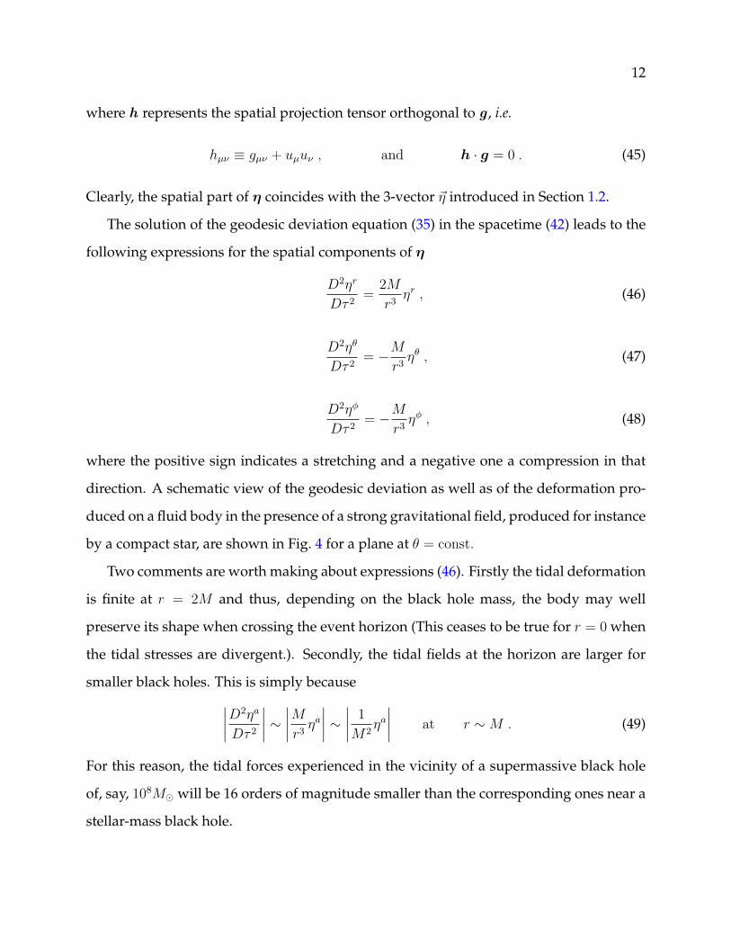
where the positive sign indicates a stretching and a negative one a compression in that

direction. A schematic view of the geodesic deviation as well as of the deformation pro-

duced on a fluid body in the presence of a strong gravitational field, produced for instance

by a compact star, are shown in Fig. 4 for a plane at θ = const.

Two comments are worth making about expressions (46). Firstly the tidal deformation

is finite at r = 2M and thus, depending on the black hole mass, the body may well

preserve its shape when crossing the event horizon (This ceases to be true for r = 0 when

the tidal stresses are divergent.). Secondly, the tidal fields at the horizon are larger for

smaller black holes. This is simply because∣∣∣∣D2ηa

Dτ 2

∣∣∣∣ ∼ ∣∣∣∣Mr3ηa

∣∣∣∣ ∼ ∣∣∣∣ 1

M2ηa

∣∣∣∣ at r ∼ M . (49)

For this reason, the tidal forces experienced in the vicinity of a supermassive black hole

of, say, 108M� will be 16 orders of magnitude smaller than the corresponding ones near a

stellar-mass black hole.

13

η

T = 0

T > 0

µν

µν

Figure 4: Schematic view of the geodesic deviation as well as of the deformation produced on a fluid body

in the presence of a strong gravitational field. In the case considered here the source of the gravitational

field is represented by a massive body (i.e. Tµν > 0) but a qualitative similar scheme would be true also in

the case of a black hole.

Appendix: Lie Derivative

That of the Lie derivative is a useful concept which lays the road for the more generic

concept of the covariant derivative. In many respects, the Lie derivative can be considered

as the extension of the directional derivative (i.e. the derivative of along a vector) to the

directional derivative in a space where the coordinates are allowed to vary.

Consider therefore a vector field V(xµ) and the family of curves having V as a tangent

vector, i.e. (cf. Fig. 1) .

V µ(xµ) ≡ dxµ

dτ, (50)

where τ is the parameter chosen for the curve (This operation is equivalent to finding the

streamlines out of velocity vector field.).

The basic idea behind the Lie derivative is then that of comparing tensors that are

“dragged” along a certain curve defined by a vector field and taking the limit for infinites-

14

V(Q)

C

T(P)

Q

P

V(P)

T(Q)

tensor dragged at Q

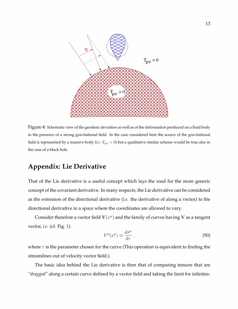
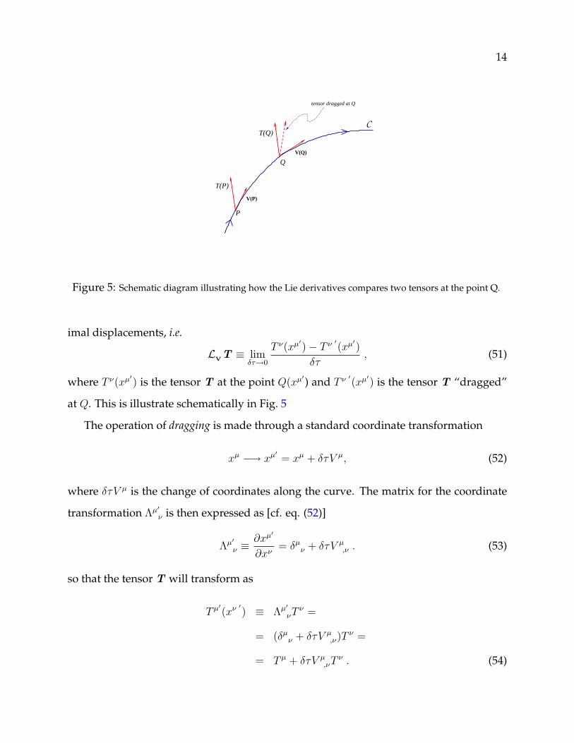
Figure 5: Schematic diagram illustrating how the Lie derivatives compares two tensors at the point Q.

imal displacements, i.e.

LVT ≡ lim

δτ→0

T ν(xµ′)− T ν ′(xµ′)

δτ, (51)

where T ν(xµ′) is the tensor T at the point Q(xµ′) and T ν ′(xµ′) is the tensor T “dragged”

at Q. This is illustrate schematically in Fig. 5

The operation of dragging is made through a standard coordinate transformation

xµ −→ xµ′ = xµ + δτV µ, (52)

where δτV µ is the change of coordinates along the curve. The matrix for the coordinate

transformation Λµ′ν is then expressed as [cf. eq. (52)]

Λµ′

ν ≡∂xµ′

∂xν= δµ

ν + δτV µ,ν . (53)

so that the tensor T will transform as

T µ′(xν ′) ≡ Λµ′

νTν =

= (δµν + δτV µ

,ν)Tν =

= T µ + δτV µ,νT

ν . (54)

15

On the other hand, T µ(x′) can be calculated through a Taylor expansion around the

point Q, thus yielding

T µ(xµ′) = T µ(xν ′) =

= T µ(xν + δxν +O((δxν)2)

)=

= T µ(xν + δτV ν +O(δτ 2)

)=

= T µ(xν) + δτV ν ∂T µ

∂xν+O(δτ 2) . (55)

Collecting now expressions (54) and (55) in the definition (51) and taking the limit for

infinitesimal displacements on the curve one obtains that the Lie derivative of T along

the vector field V is

(LVT )µ = T µ

,νVν − V µ

,νTν = L

VT µ , (56)

(LVT )µ = Tµ, νV

ν + V ν,µTν = L

VTµ . (57)

Note that in addition to the simple derivative along V (i.e. T µ,νV

ν), the Lie derivative (56)

also contains a second term (i.e. V µ,νT

ν) providing information on how the coordinates

themselves change along the curve with tangent vector V.

For a generic mixed tensor with m covariant components and n contravariant ones

(i.e. Tα1...αm

β1...βn), the Lie derivative will then be expressed as

LVTα1...αm

β1...βn= Tα1...αm

β1...βn,νVν − V α1

,νTνα2...αm

β1...βn− . . .− V αm

νTα1...αm−1ν

β1...βn−

V ,νβ1

Tα1...αm

νβ2...βn+ . . . + V ,ν

βnTα1...αm

β1...βn−1ν . (58)

1.5 Properties of the Lie derivative

1. It is a linear operator

Given two generic tensors Y , and Z , the

LV(τY αν + σZβν) = τL

VY αν + σL

VZβν . (59)

where τ and σ are two constant real coefficients.

16

2. It follows the Leibniz rule

Given two generic tensors Z , and U , then

LV(ZµνUαβ) = L

V(Zµν)Uαβ + ZµνL

VUαβ . (60)

3. It is “type-preserving”

Given a generic

m

n

-form, its Lie derivative is still a

m

n

-form

LV

m

n

form

=

m

n

form . (61)

.

4. Directional derivative

When acted upon a scalar function Φ(xα), the Lie derivative provides a directional

derivative

LVΦ = Φ,νV

ν . (62)

5. It commutes with contraction

Given a generic tensor T then

δνµ(L

VT µ

ν) = LV(δν

µTµν) = L

VT ν

ν . (63)

6. It is equivalent to the commutator operator

Given two generic tensors Y , and X (hereafter just two 4-vectors), then

LXY µ = Y µ,νX

ν −Xµ,νY

ν = [X,Y]µ . (64)

17

2 Linearized Einstein Equations

The starting point in discussing gravitational waves cannot but come from the Einstein

field equations, expressing the close equivalence between matter-energy and curvature

Gµν ≡ Rµν −1

2gµνR = 8πTµν . (65)

In the 10 linearly independent equations (65), Rµν and R are the Ricci tensor and scalar,

respectively, gµν and Gµν are the metric and Einstein tensors, respectively, while Tµν is the

stress-energy tensor of the matter in the spacetime considered.

Looking at the Einstein equations (65) as a set of second-order partial differential equa-

tions it is not easy to predict that there exist solutions behaving as waves. Indeed, and

as it will become more apparent in this Section, the concept of gravitational waves as so-

lutions of Einstein equations is valid only under some rather idealized assumptions such

as: a vacuum and asymptotically flat spacetime and a linearized regime for the gravi-

tational fields. If these assumptions are removed, the definition of gravitational waves

becomes much more difficult. In these cases, in fact, the full nonlinearity of the Einstein

equations complicates the treatment considerably and solutions can be found only nu-

merically. It should be noted, however, that in this respect gravitational waves are not

peculiar. Any wave-like phenomenon, in fact, can be described in terms of homogenous

wave equations only under very simplified assumptions such as those requiring an uni-

form “background” for the fields propagating as waves.

These considerations suggest that the search for wave-like solutions to Einstein equa-

tions should be made in a spacetime with very modest curvature and with a metric line

element which is that of flat spacetime but for small deviations of nonzero curvature, i.e.

gµν = ηµν + hµν +O([hµν ]2) , (66)

where

ηµν = diag(−1, 1, 1, 1) , (67)

18

and the linearized regime is guaranteed by the fact that

|hµν | � 1 . (68)

Is this condition verified in Cascina???

19

Fortunately, the conditions expressed by equations (66) and (68) are, at least in our

Solar system, rather easy to reproduce and, in fact, the deviation away from flat spacetime

that could be measured, for instance, on the surface of the Sun are

|hµν | ∼ |h00| 'M�

R�∼ 10−6 , (69)

and which should be compared with the equivalent value as measured on the surface of

the Earth M⊕/R⊕ ∼ 10−9.

Before writing the linearized version of the Einstein equations (65) it is necessary to

derive the linearized expression for the Christoffel symbols. In a coordinate basis (as the

one will will assume hereafter), the general expression for the affine connection is

Γµαβ =

1

2gµν(gνα,β + gβν,α − gαβ,ν) , (70)

where the partial derivatives are readily calculated as

gνα,β = ηνα,β + hνα,β = hνα,β , (71)

so that the linearized Christoffel symbols become

Γµαβ =

1

2ηµν(hνα,β + hβν,α − hαβ,ν) =

=1

2(h µ

α ,β + h µβ ,α − h ,µ

αβ ) . (72)

Note that the operation of lowering and raising the indices in expression (72) is not made

through the metric tensors gµν and gµν but, rather, through the spacetime metric tensors

ηµν and ηµν . This is just the consequence of linearized approximation and, despite this,

the spacetime is really curved!

Once the linearized Christoffel symbols have been computed, it is possible to derive

the linearized expression for the Ricci tensor which takes the form

Rµν = Γαµν,α − Γα

µα,ν

=1

2(h α

µ ,να + h αν , µα − h α

µν, α − h, µν) , (73)

20

where

h ≡ hαα = ηµαhµα , (74)

is the trace of the metric perturbations. The resulting Ricci scalar is then given by

R ≡ gµνRµν ' ηµνRµν . (75)

Making now use of (73) and (75) it is possible to rewrite the Einstein equations (65) in

a linearized form as

h αµα, ν + h α

να, µ − h αµν, α − h,µν − ηµν(h

αβαβ, − h α

,α ) = 16πTµν . (76)

Although linearized, the Einstein equations (76) do not seem yet to suggest a wave-

like behaviour. A good step in the direction of unveiling this behaviour can be made if a

more compact notation is introduced and which makes use of “trace-free” tensors defined

as

hµν ≡ hµν −1

2ηµνh , (77)

where the “bar-operator” can be applied to any symmetric tensor so that, for instance,

Rµν = Gµν and ¯hµν = hµν4. Using this notation, the linearized Einstein equations (76) take

the more compact form

− h αµν,α − ηµν h

αβαβ, + h α

να, µ = 16πTµν . (78)

It is now straightforward to recognize that the first term on the right-hand-side of

equation (78) is simply the Dalambertian (or wave) operator

h αµν,α = �hµν = −(−∂2

t + ∂2x + ∂2

y + ∂2z )hµν , (79)

where the last equality is valid for a Cartesian (t, x, y, z) coordinate system only. At this

stage the gauge freedom inherent to General Relativity can (and should) be exploited to

recast equations (79) in a more convenient form. A good way of exploiting this gauge

freedom is by choosing the metric perturbations hµν so as to eliminate the terms in (78)

4Note that the “bar” operator can in principle be applied also to the trace so that h = −h

21

that spoil the wave-like structure. Most notably, the metric perturbations can be selected

so that

hµα,α = 0 . (80)

Making use of the gauge (80), which is also known as “Lorentz” (or Hilbert) gauge, the

linearized field equations take the form

�hµν = −16πTµν . (81)

Despite they are treated in a linearized regime and with a proper choice of variables

and gauges, Einstein equations (81) do not yet represent wave-like equations if matter

is present (i.e. if Tµν 6= 0). A further and final step needs therefore to be taken and this

amounts to consider a spacetime devoid of matter, in which the Einstein equations can

finally be written as

�hµν = 0 , (82)

indicating that, in the Lorentz gauge, the “gravitational field” propagates in spacetime as

a wave perturbing flat spacetime.

Having recast the Einstein field equations in a wave-like form has brought us just half-

way towards analysing the properties of these objects. More will be needed in order to

discuss the nature and features of gravitational waves and this is what is presented in the

following Section.

22

2.1 A Wave Solution to Einstein Equations

The simplest solution to the linearized Einstein equations (82) is that of a plane wave of

the type

hµν = <{Aµν exp(iκαxα)} , (83)

where < selects the real part, A is the “amplitude tensor”, and κ is a null four-vector,

i.e. κακα = 0. In such a solution, the plane wave (83) travels in the spatial direction

~k = (κx, κy, κz)/κ0 with frequency ω ≡ κ0 = (κjκj)

1/2.

Note that the amplitude tensor A in the wave solution (83) has in principle 16−6 = 10

independent components. On the other hand, a number of considerations indicate that

there are only two dynamical degrees of freedom in General Relativity. This “excess” of

independent components can be explained simply. Firstly, A and κ cannot be arbitrary if

they have to describe a plane wave; as a result, an orthogonality condition between the

two quantities will constrain four of the ten components of A (see condition (a) below).

Secondly, while a global Lorentz gauge has been chosen [cf. equation (80)], this does

not fix completely the coordinate system of a linearized theory. A residual ambiguity, in

fact, is preserved through arbitrary ”gauge changes”, i.e. through infinitesimal coordinate

transformations that are not entirely constrained, even if a global gauge has been selected.

To better appreciate this, consider an infinitesimal coordinate transformation in terms of

a small but otherwise arbitrary displacement four-vector ξ

xα′ = xα + ξα . (84)

Applying this transformation to the linearized metric (66) generates a “new” metric tensor

that at the lowest order is

gNEW

µ′ν′ = ηµν + hOLD

µν − ξµ,ν − ξν,µ , (85)

so that the “new” and “old” perturbations are related by the following expression

hNEW

µ′ν′ = hOLD

µν − ξµ,ν − ξν,µ . (86)

23

or, alternatively, by

hNEW

µ′ν′ = hOLD

µν − ξµ,ν − ξν,µ + ηµνξα

,α . (87)

Requiring now that the new coordinates satisfy the condition (80) of the Lorentz gauge

hNEW ,ν′

µ′ν′ = 0, forces the displacement vector to be solution of the homogeneous wave

equation

ξα,ββ = 0 . (88)

As a result, the plane-wave vector with components

ξα ≡ −iCαexp(iκβxβ) , (89)

generates, through the four arbitrary constants Cα, a gauge transformation that changes

arbitrarily four components of A in addition to those coming from the condition A ·κ = 0.

Effectively, therefore, Aµν has only 10 − 4 − 4 = 2 linearly independent components,

corresponding to the number of degrees of freedom in General Relativity [1].

Note that all this is very similar to what happens in classical electrodynamics, where

the Maxwell equations are invariant under transformations of the vector potentials of the

type Aµ → Aµ′ = Aµ + Ψ,µ, so that the corresponding electromagnetic tensor FNEW

µ′ν′ =

Aµ′,ν′ − Aν′,µ′ = FOLD

µ′ν′ . Similarly, in a linearized theory of General Relativity, the gauge

transformation (86) will preserve the components of the Riemann tensor, i.e. RNEW

αβµν =

ROLD

αβµν .

To summarize, it is convenient to constrain the components of the amplitude tensor

through the following conditions:

(a): Orthogonality Condition: four components of the amplitude tensor can be specified

if A and κ are chosen to be orthogonal, i.e.

Aµνκν = 0 . (90)

(b): Global Lorentz Frame: just like in Special Relativity, a global Lorentz frame relative

24

to an observer with four-velocity u can be defined. In this case, three5 components

of the amplitude tensor can be specified after selecting a four-velocity u orthogonal

to A, i.e.

Aµνuν = 0 . (91)

(c): Infinitesimal Gauge Transformation: one final independent component in the am-

plitude tensor can be eliminated after selecting the infinitesimal displacement vector

ξµ = iCµ exp(iκαxα) so that

Aµµ = 0 . (92)

Conditions (a), (b) and (c) define the so called “Transverse and Traceless” (TT) gauge and

represent the standard gauge for the analysis of gravitational waves.

To appreciate the significance of the constraint conditions (90)–(92), consider them im-

plemented in a reference frame which is globally at rest, i.e. uα = (1, 0, 0, 0). In this frame,

the components of the wave vector κµ do not appear directly, and the above conditions

for the amplitude tensor can be written as

(a):

Aµνκν = 0 ⇐⇒ hij,j = 0 , (93)

i.e. the spatial components of hµν are divergence-free.

(b):

Aµνuν = 0 ⇐⇒ hµ0 = 0 , (94)

i.e. only the spatial components of hµν are nonzero (hence the transverse character of

the TT -gauge).

5Note that the conditions (90) fix three and not four components because one further constraint needs to

be satisfied, i.e. κµAµνuν = 0.

25

(c):

Aµµ = 0 ⇐⇒ h = hj

j = 0 , (95)

i.e. the spatial components of hµν are trace-free hence the trace-free character of the

TT -gauge). Because of this, and only in this gauge, hµν = hµν

An obvious question that might emerge at this point is about the generality of the TT

gauge. A simple answer to this question can be provided by reminding that any linear

gravitational wave can, just like any electromagnetic wave, be decomposed in the linear

superposition of planar waves. Because all of the conditions (94)–(95) are linear in hµν ,

any of the composing planar waves can be chosen to satisfy (94)–(95), which, as a result,

are satisfied also by the original gravitational wave. Indeed, all of what just stated is

contained in a theorem establishing that: once a global Lorentz frame has been chosen in

which uα = δα0, it is then always possible to find a gauge in which the conditions (94)–(95)

are satisfied.

26

2.2 Making Sense of the TT Gauge

As introduced so far, the TT gauge might appear rather abstract and not particularly in-

teresting. Quite the opposite, the TT gauge introduces a number of important advantages

and simplifications in the study of gravitational waves. The most important of these is

that, in this gauge, the only nonzero components of the Riemann tensor are

Rj0k0 = R0j0k = −Rj00k = −R0jk0 . (96)

Since, however,

Rj0k0 = −1

2h

TT

jk,00 , (97)

the use of the TT gauge indicates that a travelling gravitational wave with periodic time

behaviour hTT

jk ∝ exp(iωt) can be associated to a local oscillation of the spacetime curva-

ture, i.e.

hTT

jk,00 ∼ −ω2 exp(iωt) ∼ Rj0k0 , (98)

and thus

Rj0k0 =1

2ω2h

TT

jk . (99)

To better appreciate the effects of the propagation of a gravitational wave, it is useful

to consider the separation between two neighbouring particles A and B on a geodesic

motion and how this separation changes in the presence of an incident gravitational wave

(see Fig. 6). Note that considering a single particle would not be sufficient to establish the

effect of an incident gravitational wave. Its coordinate position does not change at the

passage of the wave and it is, indeed, the relative displacement between two adjacent

particles that allows for the detection of the measurement.

For this purpose, let us introduce a coordinate system xα in the neighbourhood of

particle A so that along the worldline of the particle A the line element will have the form

ds2 = −dτ 2 + δijdxidxj +O(|xj|2)dxαdxβ , (100)

where, of course, we are interested exactly in quantifying the O(|xj|2) terms.

27

The arrival of a gravitational wave will perturb the geodesic motion of the two par-

ticles and produce a nonzero contribution to the geodesic deviation equation. I remind

that the changes in the separation four-vector ξ between two geodesic trajectories with

tangent four-vector V are expressed through the geodesic deviation equation [cf. equa-

tion (35)]

V γV βξα;βγ = −Rα

βγδVβξγV δ , (101)

or, equivalently, as

V γV β

(D2ξα

Dτ 2

)≡ V γV β

(d2ξα

dτ 2+ Γα

βγ

dξα

dτ

dξβ

dτ

)= −Rα

βγδVβξγV δ . (102)

njA

k

k

B

Figure 6: Schematic diagram for the changes in the separation vector between two particles A and B mov-

ing along geodesic trajectories produced by the interaction with a gravitational wave propagating along the

direction ~k.

Indicating now with njB≡ hj

αξα = xjB− xj

A= xj

Bthe components of the separation

three-vector in the positions of the two particles, the geodesic deviation equation (102)

can be written asD2xj

B

Dτ 2= −Rj

0k0xk

B. (103)

28

A first simplification to these equations comes from the fact that around the particle A

the affine connections vanish (i.e. Γj

αβ= 0) and the covariant derivative in (103) can

be replaced by an ordinary total derivative. Furthermore, because in the TT gauge the

coordinate system xα moves together with the particle A, the proper and the coordinate

time coincide at first order in the metric perturbation [i.e. τ = t at O(hTT

µν )]. As a result,

equation (103) effectively becomes

d2xjB

dt2=

1

2

(∂2h

TT

jk

∂t2

)xk

B, (104)

and has solution

xjB(t) = xk

B(0)

[δjk +

1

2h

TT

jk(t)

]. (105)

Equation (105) has a straightforward interpretation and indicates that, in the reference

frame comoving with A, the particle B is seen oscillating with an amplitude proportional

to hTT

jk.

Note that because these are transverse waves, they will produce a local deformation of

the spacetime only in the plane orthogonal to their direction of propagation. As a result,

if the two particles lay along the direction of propagation (i.e. if ~n ‖ ~k), then [cf eq. (90)]

hTT

jkxj

B(0) ∝ h

TT

jkκj

B(0) = 0 , (106)

and no oscillation will be recorded by A [cf. equation (93)]

Let us now consider a concrete example and in particular a planar gravitational wave

propagating in the positive z-direction. In this case the only nonzero metric functions will

be

hTT

xx = −hTT

yy = <{A+ exp[−iω(t− z)]} , (107)

hTT

xy = hTT

yx = <{A× exp[−iω(t− z)]} , (108)

where A+ and A× represent the only two independent degrees of freedom.

29

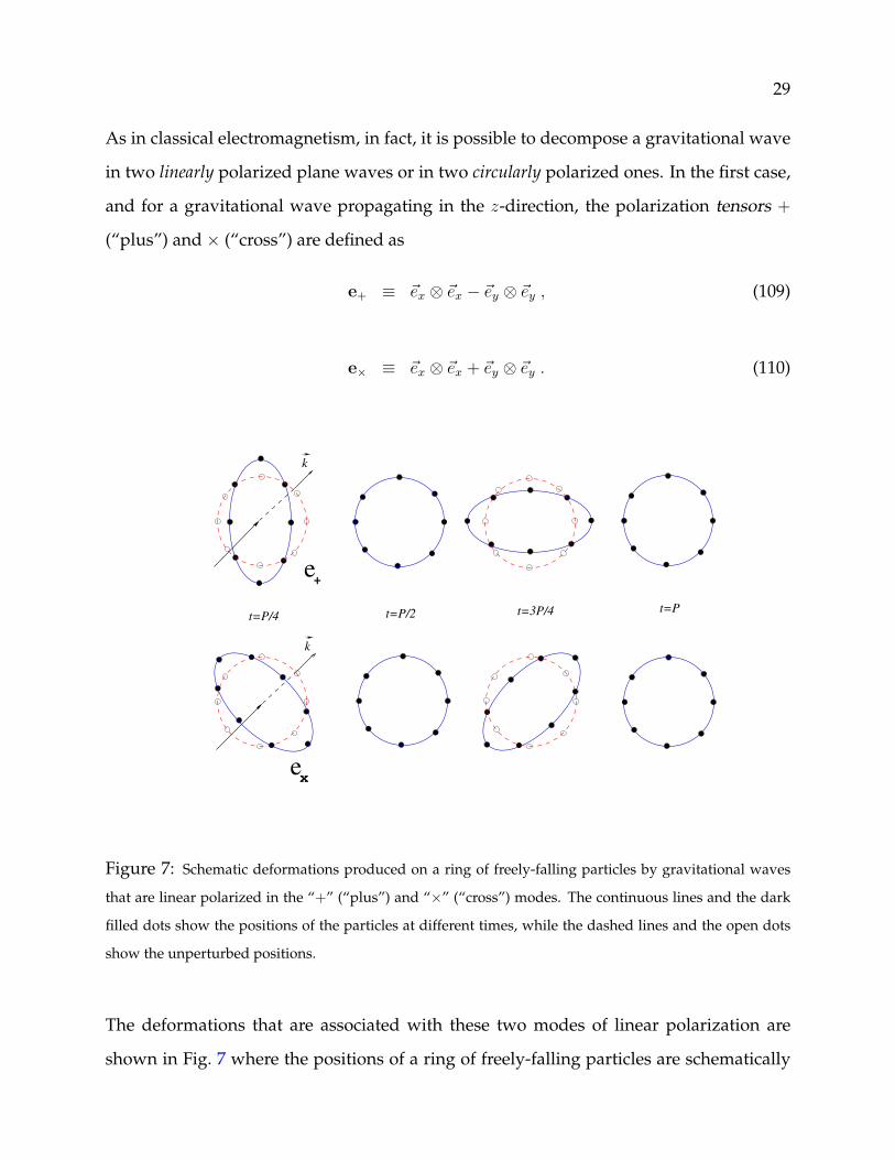
As in classical electromagnetism, in fact, it is possible to decompose a gravitational wave

in two linearly polarized plane waves or in two circularly polarized ones. In the first case,

and for a gravitational wave propagating in the z-direction, the polarization tensors +

(“plus”) and × (“cross”) are defined as

e+ ≡ ~ex ⊗ ~ex − ~ey ⊗ ~ey , (109)

e× ≡ ~ex ⊗ ~ex + ~ey ⊗ ~ey . (110)

e+

t=P/4 t=P/2 t=3P/4 t=P

ex

k

k

Figure 7: Schematic deformations produced on a ring of freely-falling particles by gravitational waves

that are linear polarized in the “+” (“plus”) and “×” (“cross”) modes. The continuous lines and the dark

filled dots show the positions of the particles at different times, while the dashed lines and the open dots

show the unperturbed positions.

The deformations that are associated with these two modes of linear polarization are

shown in Fig. 7 where the positions of a ring of freely-falling particles are schematically

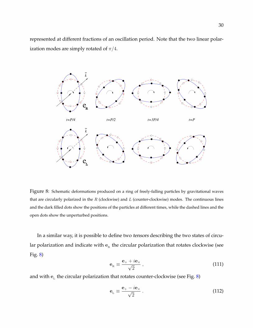
30

represented at different fractions of an oscillation period. Note that the two linear polar-

ization modes are simply rotated of π/4.

eR

eL

t=P/4 t=P/2 t=3P/4 t=P

k

k

Figure 8: Schematic deformations produced on a ring of freely-falling particles by gravitational waves

that are circularly polarized in the R (clockwise) and L (counter-clockwise) modes. The continuous lines

and the dark filled dots show the positions of the particles at different times, while the dashed lines and the

open dots show the unperturbed positions.

In a similar way, it is possible to define two tensors describing the two states of circu-

lar polarization and indicate with eR

the circular polarization that rotates clockwise (see

Fig. 8)

eR≡ e+ + ie×√

2, (111)

and with eL

the circular polarization that rotates counter-clockwise (see Fig. 8)

eL≡ e+ − ie×√

2. (112)

31

The deformations that are associated to these two modes of circular polarization are

shown in Fig. 8

2.3 Generation of Gravitational Waves

In what follows I briefly discuss the amounts of energy carried by gravitational waves and

provide simple expressions to estimate the gravitational radiation luminosity of potential

sources. Despite the estimates made here come from analogies with electromagnetism

and are based on a Newtonian description of gravity, they provide a reasonable approx-

imation to more accurate expressions from which they differ for factors of O(few). Note

also that if obtaining such a level of accuracy requires only a small effort, reaching the

accuracy necessary for a realistic detection of gravitational waves is far more difficult and

often imposes the use of numerical relativity calculations on modern supercomputers.

In classical electrodynamics, the energy emitted per unit time by an oscillating electric

dipole d is easily estimated to be

Lelectric dip. ≡(energy emitted)

(unit time)=

2

3q2x2 =

2

3(d)2 , (113)

where

d ≡ qx , and d ≡ qx , (114)

with q being the electrical charge and the number of “dots” counting the order of the

total time derivative. Equally simple is to calculate the corresponding luminosity in grav-

itational waves produced by an oscillating mass-dipole. In the case of a system of N

point-like particles of mass mA (A = 1, 2, . . . , N ), in fact, the total mass-dipole and its first

time derivative are

~d ≡N∑

A=1

mA~xA , (115)

and

~d ≡N∑

A=1

mA~xA = ~p , (116)

32

respectively. However, the requirement that the system conserves its total linear momen-

tum

~d ≡ ~p = 0 , (117)

forces to conclude that Lmass dipole = 0, i.e. that there is no mass-dipole radiation in Gen-

eral Relativity (This is equivalent to the impossibility of having electromagnetic radiation

from an oscillating electric monopole.). Next, consider the electromagnetic energy emis-

sion produced by an oscillating electric quadrupole. In classical electrodynamics, this

energy loss is given by

Lelectric quad. ≡1

20(...Q)2 =

1

20(...Qjk

...Qjk) , (118)

where

Qjk ≡N∑

A=1

qA

[(xA)j(xA)k −

1

3δjk(xA)i(xA)i

], (119)

is the electric quadrupole for a distribution of N charges (q1, q2, . . . , qN).

In close analogy with expression (118), the energy loss per unit time due to an oscillating

mass quadrupole is calculated to be

Lmass quadrupole ≡1

5〈

...I

2 〉 =1

5〈...I−jk

...I−jk〉 , (120)

where I−jk is the trace-less mass quadrupole (or “reduced” mass quadrupole), defined as

I−jk ≡N∑

A=1

mA

[(xA)j(xA)k −

1

3δjk(xA)i(xA)i

]=

∫ρ

(xjxk −

1

3δjkxix

i

)dV , (121)

and the brackets 〈 〉 indicate a time average [Clearly, the second expression in (121) refers

to a continuous distribution of particles with rest-mass density ρ.].

A crude estimate of the third derivative of the mass quadrupole of the system is given by

...I−jk ∼

(mass of the system in motion)× (size of the system)2

(time scale)3∼ MR2

τ 3∼ M〈v2〉

τ, (122)

where 〈v〉 is the mean internal velocity. Stated differently,

...I−jk ∼ Linternal , (123)

33

where Linternal is the power of the system flowing from one part of the system to the other.

As a result, the gravitational-wave luminosity in the quadrupole approximation can

be calculated to be

Lmass quadrupole ∼(

M〈v2〉τ

)2

∼(

M

R

)5

∼ (Linternal)2 , (124)

where the second equality has been derived using the Virial theorem for which the kinetic

energy is of the same order of the potential one and thus M〈v2〉 ∼ M2/R and the timescale

is set by the frequency of the fundamental mode of oscillation τ ∼ 1/f ∼√

R3/M . Note

that the apparently weird association of a luminosity to a luminosity squared is the con-

sequence of the use of geometrized units in which the power is dimensionless.

Although extremely simplified, expressions (122) and (124) contain the two most im-

portant pieces of information about the generation of gravitational waves. The first one

is that the conversion of any type of energy into gravitational waves is, in general, not

efficient. To see this it is necessary to bear in mind that expression (120) is in geometrized

units and that the conversion to conventional units occurs by multiplying (120) by the

factor L0 ≡ c5/G = 2.63 × 1059 erg s−1. On the other hand, expression (124) shows that

L � 1 and thus the gravitational-wave luminosity in conventional units is suppressed by

a coefficient of O(10−59).

The second information is about the time variation of the mass quadrupole, which can

become considerable only for very large masses moving at relativistic speeds. Clearly, these

conditions cannot be reached by sources in terrestrial laboratories, but can be easily met

by astrophysical compact objects, which therefore become the most promising sources of

gravitational radiation.

34

References

[1] C. W. Misner, K. S. Thorne and J. A. Wheeler, “Gravitation”, Freeman, NY (1974)

[2] B. F. Schutz, “An Introduction to General Relativity”, Cambrige Univ. Press, Cambridge

UK (1984)

[3] R. d’Inverno, “Introducing Einstein’s Relativity”, Oxford Univ. Press, Oxford UK (1990)

[4] S. Chandrasekhar, “The Mathematical Theory of Black Holes”, Oxford Univ. Press, Ox-

ford UK (1992)

[5] B. F. Schutz Detection of gravitational waves in Proceedings of “Astrophysical sources

of gravitational radiation”, J.A. Marck and J.P. Lasota Eds., Cambridge Univ. Press

(1996)