anisotropic poisson processes of cylinders - ulm · materials are usually modeled as homogeneous...

Methodol Comput Appl Probab (2011) 13:801–819DOI 10.1007/s11009-010-9193-8

Anisotropic Poisson Processes of Cylinders

Malte Spiess · Evgeny Spodarev

Received: 23 December 2009 / Revised: 23 June 2010 /Accepted: 25 August 2010 / Published online: 7 September 2010© Springer Science+Business Media, LLC 2010

Abstract Main characteristics of stationary anisotropic Poisson processes of cylin-ders (dilated k-dimensional flats) in d-dimensional Euclidean space are studied.Explicit formulae for the capacity functional, the covariance function, the contactdistribution function, the volume fraction, and the intensity of the surface areameasure are given which can be used directly in applications.

Keywords Porous media · Fiber process · Anisotropy · Intrinsic volumes ·Stochastic geometry

AMS 2000 Subject Classifications 60D05 · 60G10

1 Introduction

Porous fiber materials find vast applications in modern material technologies. Theiruse ranges from light polymer-based non-woven materials, see Helfen et al. (2003),to fiber-reinforced textile and fuel cells as in Mukherjee and Wang (2006). Theirporosity, percolation, acoustic absorption and liquid permeability are of specialinterest. It is known that these properties depend to a great extent on the microscopicstructure of fibers, in particular, on the orientation of a typical fiber. If all directionsof fibers are equiprobable one speaks of isotropy. Many materials are made bypressing an isotropic collection of fibers together thus producing strongly anisotropicstructures. As examples, pressed non-woven materials used as an acoustic trim incar production, see Schladitz et al. (2006), paper making process as in Corte and

M. Spiess (B) · E. SpodarevInstitute of Stochastics, Ulm University, Helmholtzstr. 18, 89069 Ulm, Germanye-mail: [email protected]

E. Spodareve-mail: [email protected]

802 Methodol Comput Appl Probab (2011) 13:801–819

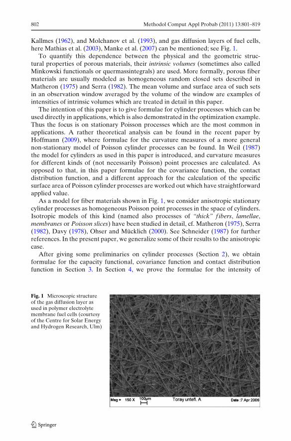
Kallmes (1962), and Molchanov et al. (1993), and gas diffusion layers of fuel cells,here Mathias et al. (2003), Manke et al. (2007) can be mentioned; see Fig. 1.

To quantify this dependence between the physical and the geometric struc-tural properties of porous materials, their intrinsic volumes (sometimes also calledMinkowski functionals or quermassintegrals) are used. More formally, porous fibermaterials are usually modeled as homogeneous random closed sets described inMatheron (1975) and Serra (1982). The mean volume and surface area of such setsin an observation window averaged by the volume of the window are examples ofintensities of intrinsic volumes which are treated in detail in this paper.

The intention of this paper is to give formulae for cylinder processes which can beused directly in applications, which is also demonstrated in the optimization example.Thus the focus is on stationary Poisson processes which are the most common inapplications. A rather theoretical analysis can be found in the recent paper byHoffmann (2009), where formulae for the curvature measures of a more generalnon-stationary model of Poisson cylinder processes can be found. In Weil (1987)the model for cylinders as used in this paper is introduced, and curvature measuresfor different kinds of (not necessarily Poisson) point processes are calculated. Asopposed to that, in this paper formulae for the covariance function, the contactdistribution function, and a different approach for the calculation of the specificsurface area of Poisson cylinder processes are worked out which have straightforwardapplied value.

As a model for fiber materials shown in Fig. 1, we consider anisotropic stationarycylinder processes as homogeneous Poisson point processes in the space of cylinders.Isotropic models of this kind (named also processes of “thick” f ibers, lamellae,membranes or Poisson slices) have been studied in detail, cf. Matheron (1975), Serra(1982), Davy (1978), Ohser and Mücklich (2000). See Schneider (1987) for furtherreferences. In the present paper, we generalize some of their results to the anisotropiccase.

After giving some preliminaries on cylinder processes (Section 2), we obtainformulae for the capacity functional, covariance function and contact distributionfunction in Section 3. In Section 4, we prove the formulae for the intensity of

Fig. 1 Microscopic structureof the gas diffusion layer asused in polymer electrolytemembrane fuel cells (courtesyof the Centre for Solar Energyand Hydrogen Research, Ulm)

Methodol Comput Appl Probab (2011) 13:801–819 803

the surface area measure of anisotropic stationary Poisson processes of cylinders.Formulae for the intensities of other intrinsic volumes can be found in the recentpaper by Hoffmann (2009). In the last section, we show how the volume fraction of ananisotropic Poisson process of cylinders can be maximized under certain constraints.In the solution, we use the formulae obtained in previous sections.

Since the formulae obtained in Sections 3 and 4 are rather complex, examplesin the most interesting dimensions 2 and 3 are given, which can be directly used inapplications.

2 Cylinder Processes

Let G(k, d) be the Grassmann manifold of all non-oriented k-dimensional linearsubspaces of R

d, and G the σ -algebra of Borel subsets of G(k, d) in its usual topology.Let C (K) be the set of all compact (compact convex) non-empty sets in R

d. Denoteby R the convex ring, i.e., the family of all finite unions of non-empty compact convexsets. We provide these sets with the Hausdorff metric, and denote the resulting Borelσ -algebra of R by R.

Denote by νk(·) the k-dimensional Lebesgue measure in Rk, and by Hk(·) the

k-dimensional Hausdorff measure. For any set S ⊂ Rd denote by S⊥ the linear

subspace of the vectors which are orthogonal to all elements of S. For ξ beinga k-dimensional flat (i.e. a k-dimensional linear subspace) we denote the (d − k)-dimensional Lebesgue measure in ξ⊥ by ν

ξ

d−k. Let κk (ωk) be the volume (surfacearea) of a unit k-dimensional ball, respectively.

For a convex set K ∈ K and x ∈ Rd let p(K, x) be the unique point in K which is

the closest to x. Then there exist measures �k(K, ·) on B(Rd), for k = 0, . . . , d with

νd({x ∈ K ⊕ Br(o) : p(K, x) ∈ B}) =d∑

k=0

rd−kκd−k�k(K, B),

where K1 ⊕ K2 = {k1 + k2|k1 ∈ K1, k2 ∈ K2}, and Br(o) is the ball of radius r cen-tered in the origin o. Furthermore we define �k(∅, B) = 0 for all B ∈ B(Rd). Thesemeasures are called curvature measures. Since they are locally determined, theycan be extended to functions with locally polyconvex sets as first argument insuch a way that they remain additive. One should remark that these generalizedcurvatures measures are not necessarily positive, but signed measures. For a detailedintroduction, see Schneider and Weil (2008). The intrinsic volumes of K can bedefined as total curvature measures Vd

k(K) = �k(K, Rd) for k = 0, . . . , d.

Following the approach introduced in Weil (1987), we define a cylinder as theMinkowski sum of a flat ξ ∈ G(k, d) and a set K ⊂ ξ⊥ with K ∈ R. Note that K isnot limited to sets with an associated point in the origin. The flat ξ is also calledthe direction space of ξ ⊕ K and K is called the cross section or base. For a cylinderZ = K ⊕ ξ we define the functions L(Z ) = ξ and K(Z ) = K. Furthermore, defineZk as the set of all cylinders which have a k-dimensional direction space and basein R. For the volume of the cross-section of the cylinder we introduce the notationA(Z ) = ν

L(Z )

d−k (K(Z )). By S(K) we denote the surface area of a set K. In the caseof K being the cross-section of a cylinder K ⊕ L we shall use this notation for thesurface area of K in the space L⊥.


We call a measure ϕ on Zk locally f inite if ϕ({Z ∈ Zk|Z ∩ K �= ∅}) < ∞ for allK ∈ C. Let M(Zk) be the set of locally finite counting measures on Zk suppliedwith the usual σ -algebra M. A point process on Zk which is a measurablemapping from a probability space (,F , P) into (M(Zk),M) is called a cylin-der process. Its distribution is given by the probability measure P : M → [0, 1],P(·) = P( ∈ ·). A cylinder process is called Poisson if (B) is Poisson distributedwith mean �(B) for some locally finite measure � on Zk and all Borel setsB ⊂ Zk, and (B1),(B2), . . . , (Bn) are independent for all disjoint Borel setsB1, B2, . . . , Bn ⊂ Zk, and all n ≥ 2, see details in Schneider and Weil (2008). Themeasure � is called the intensity measure of . The Poisson cylinder process is calledsimple, if it has no multiple points. This is the case if and only if � is diffuse. For therest of this paper we assume that is a simple Poisson cylinder process. In this case,the union U = ∪Z∈ Z is a random closed set, see Schneider and Weil (2008, p. 96),where we denote by Z ∈ the cylinders Z in the support set of .

The cylinder process is called stationary if its distribution is invariant withrespect to translations in R

d and isotropic if it is invariant w.r.t. rotations about theorigin. Let Zo

k be the set of all cylinders K ⊕ ξ with ξ ∈ G(k, d), K ⊂ ξ⊥, and forwhich the midpoint of the circumsphere of K lies in the origin.

Following Weil (1987), we define i : (x, Z ) → x + Z for x ∈ Rd and Z ∈ Zo

k . If

is stationary, then a number λ ≥ 0 and a probability measure θ on Zok exist such that

�(i(A × C)) = λ

∫

Cν

L(Z )

d−k (A)θ(dZ )

for all Borel sets A ⊂ Rd, C ⊂ Zo

k . Then λ is called the intensity and θ the shapedistribution of .

As shown in König and Schmidt (1991, p. 61), θ can be decomposed further.Analogously to i define j: (� × ξ) → � ⊕ ξ for � ∈ R and ξ ∈ G(k, d). Then thereexist a probability measure α on G (directional distribution of ) and a probabilitykernel β : R × G(k, d) → [0, 1] for which β(·, ξ) is concentrated on subsets of ξ⊥such that for arbitrary R ∈ R and G ∈ G the equation

θ( j(R × G)) =∫

Gβ(R, ξ)α(dξ) (1)

holds.

3 Capacity Functional and Related Characteristics

In this section, we calculate the capacity functional (cf. Stoyan et al. 1995, p. 195) forthe union set U of the stationary Poisson process of cylinders with k-dimensionaldirection space introduced as above. As a corollary, explicit formulae for the volumefraction, the covariance function, and the contact distribution function of U followeasily. It is worth mentioning that the resulting formula (2) for the capacity functionalgeneralizes the formula in Serra (1982, pp. 572–573), given for Poisson slices in R

3,and a model with this capacity functional has already been proposed in Matheron(1975, p. 148).


3.1 Capacity Functional

For any random closed set X, the capacity functional TX(B) = P(X ∩ B �= ∅), B ∈ C,determines uniquely the distribution of X.

Let πη(B) be the orthogonal projection of a set B ⊂ Rd along a linear subspace

η ⊂ Rd onto η⊥.

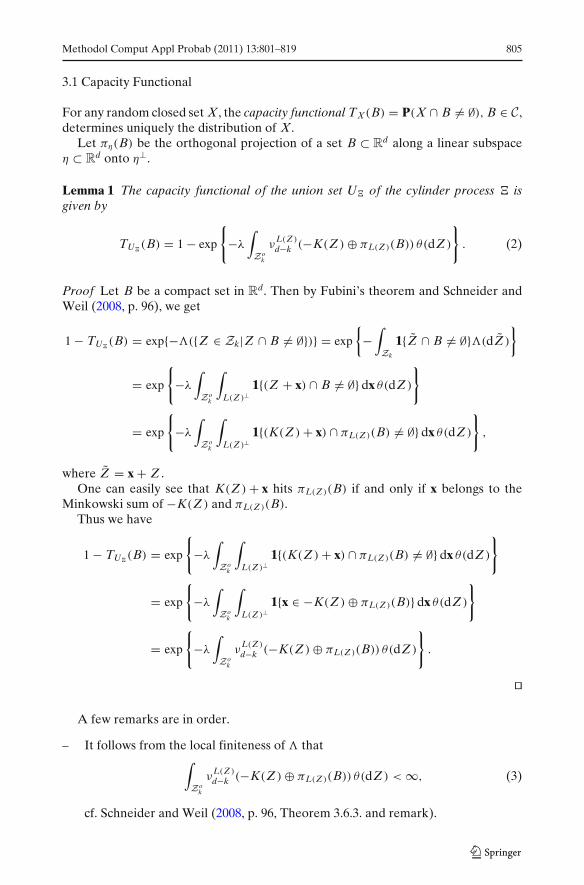
Lemma 1 The capacity functional of the union set U of the cylinder process isgiven by

TU(B) = 1 − exp

{−λ

∫

Zok

νL(Z )

d−k (−K(Z ) ⊕ πL(Z )(B)) θ(dZ )

}. (2)

Proof Let B be a compact set in Rd. Then by Fubini’s theorem and Schneider and

Weil (2008, p. 96), we get

1 − TU(B) = exp{−�({Z ∈ Zk|Z ∩ B �= ∅})} = exp

{−

∫

Zk

1{Z̃ ∩ B �= ∅}�(dZ̃ )

}

= exp

{−λ

∫

Zok

∫

L(Z )⊥1{(Z + x) ∩ B �= ∅} dx θ(dZ )

}

= exp

{−λ

∫

Zok

∫

L(Z )⊥1{(K(Z ) + x) ∩ πL(Z )(B) �= ∅} dx θ(dZ )

},

where Z̃ = x + Z .One can easily see that K(Z ) + x hits πL(Z )(B) if and only if x belongs to the

Minkowski sum of −K(Z ) and πL(Z )(B).Thus we have

1 − TU(B) = exp

{−λ

∫

Zok

∫

L(Z )⊥1{(K(Z ) + x) ∩ πL(Z )(B) �= ∅} dx θ(dZ )

}

= exp

{−λ

∫

Zok

∫

L(Z )⊥1{x ∈ −K(Z ) ⊕ πL(Z )(B)} dx θ(dZ )

}

= exp

{−λ

∫

Zok

νL(Z )

d−k (−K(Z ) ⊕ πL(Z )(B)) θ(dZ )

}.

��

A few remarks are in order.

– It follows from the local finiteness of � that∫

Zok

νL(Z )

d−k (−K(Z ) ⊕ πL(Z )(B)) θ(dZ ) < ∞, (3)

cf. Schneider and Weil (2008, p. 96, Theorem 3.6.3. and remark).


– The choice of k = 0 yields the capacity functional of the stationary BooleanModel ′ with the primary grain K and intensity λ, cf. Matheron (1975, p. 62):

T′(B) = 1 − e−λEνd(−K⊕B) .

– Another important special case is that of K being a.s. a point. Then the modelcoincides with a k-flat process ′′, cf. Matheron (1975, p. 67) with the capacityfunctional

T′′(B) = 1 − exp

{−λ

∫

Zok

νL(Z )

d−k (πL(Z )(B)) θ(dZ )

}.

– The case of B = {o} yields the volume fraction p = P(o ∈ U) = Eνd(U ∩[0, 1]d) of U:

p = TU({o}) = 1 − exp

{−λ

∫

Zok

A(Z ) θ(dZ )

}. (4)

A generalization of this formula can also be found in Hoffmann (2009) in thenon-stationary setting.Throughout this paper, we assume that p > 0, i.e.

∫Zo

kA(Z )θ(dZ ) > 0. Thus, we

have p ∈ (0, 1), cf. inequality (3).

3.2 Covariance Function

In the following we investigate the covariance function of U. It is defined asCU

(h) = P(o, h ∈ ), h ∈ Rd, cf. Stoyan et al. (1995, p. 68).

Because of the relation CU(h) = P(o, h ∈ ) = 2p − TU

({o, h}) it is closelyconnected with the capacity functional of the set B = {o, h}, which is

TU({o, h}) = 1 − exp

{−λ

∫

Zok

νL(Z )

d−k ({o, πL(Z )(h)} ⊕ −K(Z )) θ(dZ )

}. (5)

Let γA denote the covariogram of a measurable set A ⊂ L(Z )⊥ defined by

γA(x) = νL(Z )

d−k (A ∩ (A − x))

for x ∈ L(Z )⊥.

Lemma 2 For h ∈ Rd we have

CU(h) = 1 − 2 exp

{−λ

∫

Zok

A(Z ) θ(dZ )

}

+ exp

{−2λ

∫

Zok

A(Z ) θ(dZ ) + λ

∫

Zok

γK(Z )(πL(Z )(h)) θ(dZ )

}. (6)


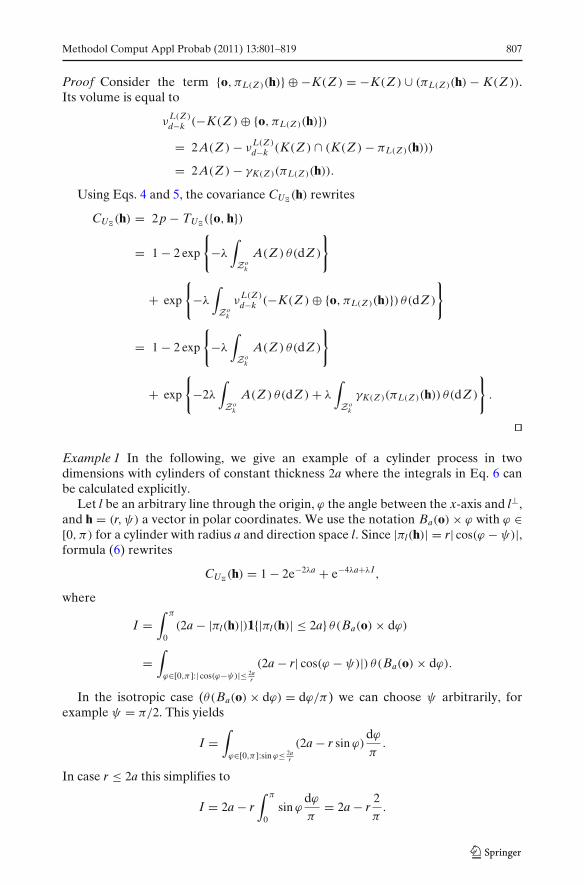
Proof Consider the term {o, πL(Z )(h)} ⊕ −K(Z ) = −K(Z ) ∪ (πL(Z )(h) − K(Z )).Its volume is equal to

νL(Z )

d−k (−K(Z ) ⊕ {o, πL(Z )(h)})= 2A(Z ) − ν

L(Z )

d−k (K(Z ) ∩ (K(Z ) − πL(Z )(h)))

= 2A(Z ) − γK(Z )(πL(Z )(h)).

Using Eqs. 4 and 5, the covariance CU(h) rewrites

CU(h) = 2p − TU

({o, h})

= 1 − 2 exp

{−λ

∫

Zok

A(Z ) θ(dZ )

}

+ exp

{−λ

∫

Zok

νL(Z )

d−k (−K(Z ) ⊕ {o, πL(Z )(h)}) θ(dZ )

}

= 1 − 2 exp

{−λ

∫

Zok

A(Z ) θ(dZ )

}

+ exp

{−2λ

∫

Zok

A(Z ) θ(dZ ) + λ

∫

Zok

γK(Z )(πL(Z )(h)) θ(dZ )

}.

��

Example 1 In the following, we give an example of a cylinder process in twodimensions with cylinders of constant thickness 2a where the integrals in Eq. 6 canbe calculated explicitly.

Let l be an arbitrary line through the origin, ϕ the angle between the x-axis and l⊥,and h = (r, ψ) a vector in polar coordinates. We use the notation Ba(o) × ϕ with ϕ ∈[0, π) for a cylinder with radius a and direction space l. Since |πl(h)| = r| cos(ϕ − ψ)|,formula (6) rewrites

CU(h) = 1 − 2e−2λa + e−4λa+λI,

where

I =∫ π

0(2a − |πl(h)|)1{|πl(h)| ≤ 2a} θ(Ba(o) × dϕ)

=∫

ϕ∈[0,π]:| cos(ϕ−ψ)|≤ 2ar

(2a − r| cos(ϕ − ψ)|) θ(Ba(o) × dϕ).

In the isotropic case (θ(Ba(o) × dϕ) = dϕ/π) we can choose ψ arbitrarily, forexample ψ = π/2. This yields

I =∫

ϕ∈[0,π]:sin ϕ≤ 2ar

(2a − r sin ϕ)dϕ

π.

In case r ≤ 2a this simplifies to

I = 2a − r∫ π

0sin ϕ

dϕ

π= 2a − r

2

π.


And for r > 2a we get

I = 2aπ

(∫ arcsin 2ar

0dϕ +

∫ π

π−arcsin 2ar

dϕ

)

+ rπ

(∫ arcsin 2ar

0(− sin ϕ) dϕ +

∫ π

π−arcsin 2ar

(− sin ϕ) dϕ

)

= 4aπ

arcsin

(2ar

)+ 2r

π

(cos

(arcsin

(2ar

))− 1

)

= 2a − 4aπ

arccos

(2ar

)− 2r

π

⎛

⎝1 −√

1 −(

2ar

)2⎞

⎠ ,

which gives us the final formula

CU(h) =

⎧⎪⎪⎪⎪⎨

⎪⎪⎪⎪⎩

1 − 2e−2λa + e−2λa− 2λrπ , if r ≤ 2a,

1 − 2e−2λa + exp

{− 2λa−

− λπ

(4a arccos

(2ar

) + 2r(

1 −√

1 − 4a2

r2

))}, if r > 2a.

The first derivative of CU(h) will be needed later for the calculation of the

intensity S of the surface area measure of U.

Proposition 1 Suppose that is a simple stationary Poisson cylinder process withshape distribution θ and

∫Zo

kS(K(Z ))θ(dZ ) < ∞. Then the derivative of the covari-

ance function in direction h at the origin is given by

C′U

(o, h) = λ exp

{−λ

∫

Zok

A(Z ) θ(dZ )

}∫

Zok

γ ′K(Z )(o, πL(Z )(h)) [h, L(Z )] θ(dZ ),

where γ ′A(o, η) denotes the derivative of γA at the origin in direction η, and [ξ, η] is

the volume of the parallelepiped spanned over the orthonormal bases of the linearsubspaces of ξ and η.

Proof To simplify the notation, we shall also write [x, η] for [ξ, η] if ξ is the linespanned by x. By Eq. 4, we have

CU(o) = p = 1 − exp

{−λ

∫

Zok

A(Z ) θ(dZ )

}

and thus

CU(h) − CU

(o) = exp

{−λ

∫

Zok

A(Z ) θ(dZ )

}(eJ − 1),

where

J = λ

∫

Zok

[γK(Z )(πL(Z )(h)) − A(Z )] θ(dZ ).


We observe that A(Z ) − νL(Z )

d−k (K(Z ) ∩ (K(Z ) − πL(Z )(h))) is equal to zero ifπL(Z )(h) = o, and is less than or equal to |πL(Z )(h)|S(K(Z )), otherwise.

This yields

|J| ≤ λ|h|∫

Zok

S(K(Z )) θ(dZ ) = O(|h|), h → o.

Thus we obtain eJ − 1 = J + o(J) = J + o(|h|) for h → o, and

C′U

(o, h) = limh→o

CU(h) − CU

(o)

|h| = exp

{−λ

∫

Zok

A(Z ) θ(dZ )

}(limh→o

J|h|

).

So we need to investigate the behavior of J/|h| as h → o. By the dominatedconvergence theorem, we get

limh→o

J|h| = λ

∫

Zok

limh→o

(ν

L(Z )

d−k (K(Z ) ∩ (K(Z ) − πL(Z )(h))) − A(Z )

|h||πL(Z )(h)| |πL(Z )(h)|

)θ(dZ )

= λ

∫

Zok

limt→o

(ν

L(Z )

d−k (K(Z ) ∩ (K(Z ) − t)) − A(Z )

|t|)

| cos ∠(h, L(Z )⊥)| θ(dZ )

= λ

∫

Zok

γ ′K(Z )(o, t) [h, L(Z )] θ(dZ ),

where |πL(Z )(h)|/|h| = | cos ∠(h, L(Z )⊥)|, t = πL(Z )(h), and ∠(h, L(Z )⊥) is the an-gle between vector h and plane L(Z )⊥. ��

3.3 Contact Distribution Function

Let B be an arbitrary compact set with o ∈ B (called the structuring element), andlet r > 0. The contact distribution function (cf. Stoyan et al. 1995, p. 71) HB(r) =P(U ∩ rB �= ∅ | o /∈ U) of the union set of the stationary Poisson cylinder process with structuring element B and volume fraction p ∈ (0, 1) can be calculated asfollows:

HB(r) = 1 − P(U ∩ rB = ∅)

1 − p= 1 − 1 − TU

(rB)

1 − p

= 1 −exp

{−λ

∫Zo

kν

L(Z )

d−k (−K(Z ) ⊕ πL(Z )(rB)) θ(dZ )}

exp{−λ

∫Zo

kA(Z ) θ(dZ )

}

= 1 − exp

{−λ

∫

Zok

[ν

L(Z )

d−k (−K(Z ) ⊕ πL(Z )(rB)) − A(Z )]

θ(dZ )

}. (7)

Further simplification of this formula is possible in some special cases.Consider the contact distribution function HB with B being a line segment

between the origin and a unit vector η. In this special case the contact distributionfunction is called linear. With a slight abuse of notation we shall use a vector torepresent the line segment between the origin and the endpoint of the vector. It willbe clear from the context whether the vector or the line segment is meant.


Lemma 3 If the probability kernel β(·, ξ) (cf. Eq. 1) is concentrated on convex bodiesand isotropic in the f irst argument for all ξ ∈ G(k, d) then for a unit vector η the linearcontact distribution function of U is given by

Hη(r) = 1 − e−λrCo(η) (8)

with

Co(η) = cd,k

∫

G(k,d)

∫

K∩ξ⊥S(K)β(dK, ξ)[ξ, η]α(dξ),

cd,k = ωd−k+1

2πωd−k, and K ∩ ξ⊥ denotes the family of all convex bodies in ξ⊥.

Proof 1 It follows from Eq. 7 that Eq. 8 holds iff

r Co(η) =∫

Zok

[ν

L(Z )

d−k (−K(Z ) ⊕ πL(Z )(rη)) − A(Z )]

θ(dZ ).

Using the notation introduced in Schneider (1993, p. 275–279) for mixed volumes(here all mixed volumes and surface measures are w.r.t. L(Z )⊥) we calculate

νL(Z )

d−k (−K(Z ) ⊕ πL(Z )(rη)) − A(Z )

= (d − k)V(πL(Z )(rη), K(Z ), . . . , K(Z ))

= r2

∫

Sd−1∩L(Z )⊥|〈u, πL(Z )(η)〉| Sd−k−1(K(Z ), du),

where 〈·, ·〉 denotes the scalar product, and Sd−k−1(K(Z ), ·) is the surface areameasure of K(Z ) in L(Z )⊥.

Thus,

Co(η) = 1

2

∫

Zok

∫

Sd−1∩L(Z )⊥|〈u, πL(Z )(η)〉| Sd−k−1(K(Z ), du) θ(dZ )

= 1

2

∫

G(k,d)

∫

K∩ξ⊥

∫

Sd−1∩ξ⊥|〈u, πξ (η)〉| Sd−k−1(K, du) β(dK, ξ) α(dξ).

Because of the rotation invariance of β(·, ξ), the value of the integral does notchange if we replace K with ϑ K for an arbitrary rotation ϑ in ξ⊥. Furthermore, weget the following equation since the surface area measure is invariant w.r.t. rotationswhen they are applied to both arguments.

∫

Sd−1∩ξ⊥|〈u, πξ (η)〉| Sd−k−1(ϑ K, du) =

∫

Sd−1∩ξ⊥|〈ϑu, πξ (η)〉| Sd−k−1(K, du).


Thus, integration over the group rot(ξ⊥) of rotations in ξ⊥ equipped with the Haarprobability measure leads to

∫

Sd−1∩ξ⊥|〈u, πξ (η)〉| Sd−k−1(K, du)

=∫

rot(ξ⊥)

∫

Sd−1∩ξ⊥|〈u, πξ (η)〉| Sd−k−1(K, du) dϑ

=∫

Sd−1∩ξ⊥

∫

rot(ξ⊥)

|〈ϑu, πξ (η)〉| dϑ Sd−k−1(K, du)

= 2cd,k S(K)[ξ, η],where cd,k is the constant from the claim, and we used Spodarev (2002, Corollary 5.2)for the last equality.

This leads to

Co(η) = cd,k

∫

G(k,d)

∫

K∩ξ⊥S(K)β(dK, ξ)[ξ, η]α(dξ).

��

Now let the structuring element B be the ball B1(o). In this case the contactdistribution function is called spherical. It is obvious that πL(Z )(Br(o)) is a ball ofradius r in the (d − k)-dimensional subspace L(Z )⊥. If K(Z ) is almost surely convexthen the use of the classical Steiner formula leads to

EνL(Z )

d−k (−K(Z ) ⊕ πL(Z )(Br(o))) = EA(Z ) +d−k∑

i=1

κi EVd−kd−k−i(K(Z ))ri,

which yields

HB1(o)(r) = 1 − exp

{−λ

d−k∑

i=1

κiri∫

Zok

Vd−kd−k−i(K(Z )) θ(dZ )

}.

Example 2 In what follows, the case of dimensions two and three is considered indetail. It is assumed that the conditions of Lemma 3 hold.

– For d = 2, k = 1 Lemma 3 yields

Co(η) = c2,1

∫

G(1,2)

∫

K∩ξ⊥S(K)β(dK, ξ)[ξ, η]α(dξ) =

∫

G(1,2)

2[ξ, η]α(dξ).

Hence, it holds Hη(r) = 1 − exp{−2λ r

∫G(1,2)

[ξ, η]α(dξ)}

, and so Hη(r) does notdepend on K(Z ).And for the structuring element being B = B1(o) one gets

HB1(o)(r) = 1 − exp

{−2λ r

∫

Zo1

V10(K(Z )) θ(dZ )

}= 1 − e−2λ r.

Interestingly the result does not depend on the distribution of the cross section.


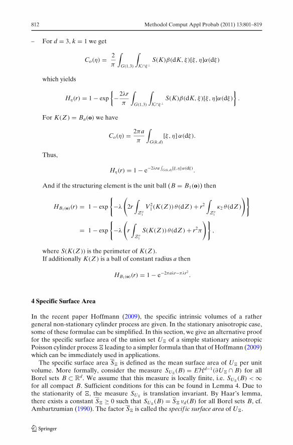
– For d = 3, k = 1 we get

Co(η) = 2

π

∫

G(1,3)

∫

K∩ξ⊥S(K)β(dK, ξ)[ξ, η]α(dξ)

which yields

Hη(r) = 1 − exp

{−2λr

π

∫

G(1,3)

∫

K∩ξ⊥S(K)β(dK, ξ)[ξ, η]α(dξ)

}.

For K(Z ) = Ba(o) we have

Co(η) = 2πaπ

∫

G(k,d)

[ξ, η] α(dξ).

Thus,

Hη(r) = 1 − e−2λra∫

G(k,d)[ξ,η]α(dξ).

And if the structuring element is the unit ball (B = B1(o)) then

HB1(o)(r) = 1 − exp

{−λ

(2r

∫

Zo1

V21(K(Z )) θ(dZ ) + r2

∫

Zo1

κ2 θ(dZ )

)}

= 1 − exp

{−λ

(r∫

Zo1

S(K(Z )) θ(dZ ) + r2π

)},

where S(K(Z )) is the perimeter of K(Z ).If additionally K(Z ) is a ball of constant radius a then

HB1(o)(r) = 1 − e−2πaλr−πλr2.

4 Specific Surface Area

In the recent paper Hoffmann (2009), the specific intrinsic volumes of a rathergeneral non-stationary cylinder process are given. In the stationary anisotropic case,some of these formulae can be simplified. In this section, we give an alternative prooffor the specific surface area of the union set U of a simple stationary anisotropicPoisson cylinder process leading to a simpler formula than that of Hoffmann (2009)which can be immediately used in applications.

The specific surface area S is defined as the mean surface area of U per unitvolume. More formally, consider the measure SU

(B) = EHd−1(∂U ∩ B) for allBorel sets B ⊂ R

d. We assume that this measure is locally finite, i.e. SU(B) < ∞

for all compact B. Sufficient conditions for this can be found in Lemma 4. Due tothe stationarity of , the measure SU

is translation invariant. By Haar’s lemma,there exists a constant S ≥ 0 such that SU

(B) = S νd(B) for all Borel sets B, cf.Ambartzumian (1990). The factor S is called the specif ic surface area of U.


Lemma 4 The specif ic surface area S of the union set U of a stationary anisotropiccylinder process is f inite if

∫Zo

kS(K(Z ))θ(dZ ) < ∞.

Proof Let B := B1(o) be the unit ball about the origin. Then we calculate using theabbreviation Lo = L(Zo) and Campbell’s theorem

SU(B) = EHd−1(∂U ∩ B) ≤ E

∑

Z∈

Hd−1(∂ Z ∩ B) =∫

Zk

Hd−1(∂ Z ∩ B)�(dZ )

= λ

∫

Zok

∫

L⊥o

Hd−1((∂ Zo + x) ∩ B) νLod−k(dx) θ(dZo)

= λ

∫

Zok

∫

L⊥o

∫

∂ Zo+x1B(y)Hd−1(dy) ν

Lod−k(dx) θ(dZo)

= λ

∫

Zok

∫

L⊥o

∫

∂ Zo

1B(y + x)Hd−1(dy) νLod−k(dx) θ(dZo)

≤ λ

∫

Zok

∫

∂ Zo

∫

L⊥o

1πL⊥o

(B)(πL⊥o(y))1πLo (B)(πLo(y) + x)ν

Lod−k(dx)Hd−1(dy) θ(dZo)

= λ

∫

Zok

∫

∂ Zo

1πL⊥o

(B)(πL⊥o(y))ν

Lod−k(πLo(B))Hd−1(dy) θ(dZo)

= λνLod−k(πLo(B))

∫

Zok

Hd−1(∂ Zo ∩ (πL⊥o(B) × L⊥

o )) θ(dZo)

= λκd−k

∫

Zok

νL⊥

od−k(πL⊥

o(B))Hd−k−1(∂K(Zo)) θ(dZo)

= λκkκd−k

∫

Zok

S(K(Zo)) θ(dZo).

This yields S = SU(B)/νd(B) < ∞. ��

The following results hold for any random closed set X with realizations almostsurely from the extended convex ring S which is defined as the family of sets B withB ∩ W ∈ R for any convex compact observation window W.

Lemma 5 Let X ∈ S be an arbitrary stationary random closed set with f inite specif icsurface area. Then the specif ic surface area of X is given by

SX = dκd

κd−1

∫

G(1,d)

λ(ξ)dξ, (9)

where dξ is the Haar probability measure on G(1, d), λ(ξ) = 12 E�0(X ∩ ξ, B1(o) ∩ ξ)

is the intensity of the number of connected components of X ∩ ξ on a line ξ ∈ G(1, d).


Proof By Crofton’s formula for polyconvex sets (cf. Schneider and Weil 2008,Th. 6.4.3) and Fubini’s theorem, we have

SX = 1

κdEHd−1(∂ X ∩ B1(o)) = 2

κdE�d−1(X, B1(o))

= 2�( d+12 )

√π

κd�(d/2)E

∫

G(1,d)

∫

ξ⊥�0(X ∩ (ξ + x), B1(o) ∩ (ξ + x))ν

ξ

d−1(dx)dξ

= dκd

κd−1

∫

G(1,d)

1

2E�0(X ∩ ξ, B1(o) ∩ ξ)dξ.

��

The following result generalizes the well-known formula

SX = − dκd

κd−1C′

X(0) (10)

Stoyan et al. (1995, p. 204), for stationary, isotropic, and a.s. regular random closedsets X ∈ S to the anisotropic case. A closed set is called regular if it coincides withthe closure of its interior. Note that, since in the isotropic case CX(h), h ∈ R

d dependsonly on the length of h, and not on h itself, in this formula CX is a function of a realvariable, namely the length of h. For the particular case of stationary anisotropicrandom sets in R

3 formula (11) can also be found (without a rigorous proof) inBerryman (1987).

Theorem 1 Let X be an a.s. regular stationary random closed set with realizationsfrom S and f inite specif ic surface area. If CX(h) is its covariance function then thespecif ic surface area of X is given by the formula

SX = − dκd

κd−1

∫

G(1,d)

C′X(o, rξ )dξ, (11)

where C′X(h, v) is the derivative of CX(h) at h in direction of unit vector v, and rξ is a

direction unit vector of a line ξ ∈ G(1, d).

Proof For a stationary random closed set U ⊂ R from the extended convex ringdenote by −U the set reflected at the origin. Define a random variable V which isuniformly distributed on {−1, 1} and independent of U . The random closed set UV isobviously isotropic, and thus formula (10) yields SUV = −2C′

UV(0). Since SU = SUV

and C′U (0) = C′

UV(0), this means that SU = −2C′U (0).

Applying this to U = X ∩ ξ , ξ ∈ G(1, d), we get λ(ξ) = 12 SX∩ξ = −C′

X∩ξ (0) =−C′

X(o, rξ ). Lemma 5 completes the proof. ��

If X is an a.s. regular two-dimensional stationary random closed set with realiza-tions in S , formula (11) simplifies to

SX = −π

∫ π

0C′

X(o, ϕ)dϕ

π= −

∫ π

0C′

X(o, ϕ)dϕ.

The following result is a direct corollary of Proposition 1, Theorem 1, and Fubini’stheorem.


Corollary 1 Let be a stationary Poisson cylinder process with intensity λ, shapedistribution θ and cylinders with regular cross-section K(Z ) ∈ R for θ -almost all Z ∈Zk and f inite specif ic surface area. Then, the specif ic surface area of U is given bythe formula

S = −λκddκd−1

∫

Zok

∫

G(1,d)

γ ′K(Z )(o, πL(Z )(rξ )) [ξ, L(Z )] dξ θ(dZ )

× exp

{−λ

∫

Zok

A(Z ) θ(dZ )

}.

Example 3 Assume that K(Z ) is convex and regular for θ -almost all Z ∈ Zk.

– For arbitrary d, and k = d − 1 it holds for dξ -a.e. line ξ ∈ G(1, d) that

γ ′K(Z )(o, πL(Z )(rξ )) = −1

and∫

G(1,d)

[ξ, L(Z )] dξ =∫

G(d−1,d)

[ξ⊥, L(Z )] dξ = (d + 1)κd+1κ1

dκd2κ2= (d + 1)κd+1

dκdπ,

see Spodarev (2002, Corollary 5.2).This yields

S = λ(d + 1)κd+1

πκd−1exp

{−λ

∫

Zod−1

νL(Z )1 (K(Z )) θ(dZ )

}

= 2λ exp

{−λ

∫

Zod−1

νL(Z )1 (K(Z )) θ(dZ )

}.

– For d = 3, k = 1, K = Ba(o) it can be calculated that γ ′K(Z )(o, πL(Z )(ξ)) = −πa,∫

G(1,3)[ξ, L(Z )] dξ = 1/2 (see also Stoyan et al. 1995, p. 298, or Spodarev 2002,

Corollary 5.2), and thus we have

S = 4λ1

2πae−λπa2 = 2πaλe−λπa2

,

which coincides with the case of isotropic cylinders, compare Ohser and Mück-lich (2000, p. 64).

5 Optimization Example

In this section we show how the formulae from Sections 3 and 4 can be applied tosolve an optimization problem for cylinder processes.

The following problem originates from the fuel cell research. The gas diffusionlayer of a polymer electrolyte membrane fuel cell is a porous material made ofpolymer fibers (see Fig. 1) which can be modeled well by an anisotropic Poissonprocess of cylinders in R

3. In a gas diffusion layer, the volume fraction of thepolymer material lies between 70 and 80%, and the directional distribution of fibersis concentrated on a small neighborhood of a great circle of a unit sphere S2, i.e.


all fibers are almost horizontal. In order to optimize the water and gas transportproperties, it is desirable to have a relatively small variation of the size of pores inthe medium, where we define a pore at a point x in the complement of U as themaximal ball with center in x which does not hit U.

We investigate the following mathematical simplification of this problem, whichcan be solved analytically in some particular cases.

For a fixed intensity λ of the Poisson cylinder process , find a shape distributionof cylinders θ which maximizes the volume fraction p of U provided that thevariance of the typical pore radius H is small. In other words, solve the optimizationproblem

{p → maxθ ,

VarH < ε,(12)

where H is a random variable with distribution function HB1(o)(r).As it will be clear later, the condition on the directional distribution α of fibers that

all fibers are almost horizontal can be neglected since the directional component ofthe shape distribution θ has no influence on the solution.

To simplify the notation, let cs = ∫Zo

1S(K(Z ))θ(dZ ) and �(x) be the distribution

function of a standard normally distributed random variable.First we take a look at the moments of the pore radius H (assuming that r ≥ 0),

remembering that HB1(o)(r) = 1 − e−λ(rcs+r2π) (as shown in an example in Section 3.3)and thus the density of H is equal to d

dr HB1(o)(r) = λ(cs + 2πr)e−λ(rcs+r2π). It holds

EH =∫ ∞

0rλ(cs + 2πr) exp

(−πλ

(r + cs

2π

)2)

exp

(c2

s λ

4π

)dr

= exp

(c2

s λ

4π

)λ

∫ ∞

cs2π

(r − cs

2π

)(2πr) e−πλr2

dr

= exp

(c2

s λ

4π

)1√λ

(1 − �

(cs

√λ

2π

)).

Furthermore it can be calculated that

EH2 = exp

(c2

s λ

4π

)λ

∫ ∞

0r2(cs + 2πr) exp

(−πλ

(r + cs

2π

)2)

dr

= 1

πλ− exp

(c2

s λ

4π

)cs

π√

λ

(1 − �

(cs

√λ

2π

)).

Defining ce = exp(

c2s λ

4π

)and c� =

(1 − �

(cs

√λ

2π

)), this leads to

EH2 − (EH)2 = 1

πλ− cec�cs

π√

λ− c2

ec2�

λ≤ ε,

multiplication with πλ yields the equivalent condition

1 − √λcec�cs − πc2

ec2� ≤ επλ,


which holds if and only if(

cec� +√

λcs

2π

)2

− λc2s

4π2+ (ελ − 1/π) ≥ 0.

This is always fulfilled if ε ≥ 1πλ

and λc2s

4π2 − (ελ − 1/π) ≤ 0 or, equivalently, cs ≤2π

√ε − 1

πλ.

In the following we always assume that ε ≥ 1πλ

and replace the conditionVarH < ε by a stronger sufficient condition

cs =∫

Zo1

S(K(Z ))θ(dZ ) ≤ 2π

√ε − 1

πλ. (13)

Hence, Eq. 12 is reduced to the optimization problem⎧⎨

⎩

∫Zo

1A(Z )θ(dZ ) → maxθ ,

∫Zo

1S(K(Z ))θ(dZ ) ≤ 2π

√ε − 1

πλ.

(14)

The solution of the optimization problem (14) yields cylinders with θ -a.s. circularbase. Notice that this solution does not depend on the directional distributioncomponent α of θ . Indeed, cylinders Z can be replaced by cylinders Z ′ which havethe same direction space and surface area (S(K(Z )) = S(K(Z ′))) but are circular.Then the isoperimetric inequality yields A(Z ′) ≥ A(Z ). Thus, it holds that

∫

Zo1

S(K(Z ))θ(dZ ) =∫

Zo1

S(K(Z ′))θ(dZ )

and∫

Zo1

A(Z )θ(dZ ) ≤∫

Zo1

A(Z ′)θ(dZ ),

which means that the circular version is at least not worse than the original version.Thus, we assume that the cylinders are θ -a.s. circular and denote the radius of a

cylinder Z by R(Z ). It follows from condition (13) that∫

Zo1

S(K(Z ))θ(dZ ) = 2π

∫

Zo1

R(Z )θ(dZ ) ≤ 2π

√ε − 1

πλ,

i.e. the new condition is that the expectation of the radius of a typical cylinder is less

or equal than√

ε − 1πλ

.Furthermore, it follows from Eq. 14 that maximizing p is equivalent to maximizing∫

Zo1

R(Z )2 θ(dZ ).The above calculation shows that the volume fraction of 70%–80% in the opti-

mized gas diffusion layer of a fuel cell can be achieved best by taking fibers withcircular cross sections, relatively small mean radius and high variance of this radius.

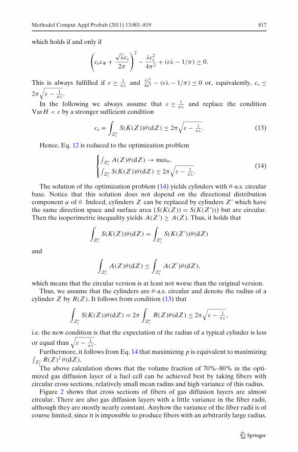
Figure 2 shows that cross sections of fibers of gas diffusion layers are almostcircular. There are also gas diffusion layers with a little variance in the fiber radii,although they are mostly nearly constant. Anyhow the variance of the fiber radii is ofcourse limited, since it is impossible to produce fibers with an arbitrarily large radius.


Fig. 2 Microscopic pictureof the gas diffusion layer

We have to remark that from a practical point of view the optimization prob-lem (12) is not well posed. For the construction of gas diffusion layers, mainly theintensity of the fibers λ can be varied. Hence a practically relevant optimizationshould involve maximizing the volume fraction p with respect to λ as well. Sincethe latter problem is much more involved than the one discussed here, it would gobeyond the scope of this paper.

Acknowledgements We would like to thank Werner Nagel, Rolf Schneider, Dietrich Stoyan,Wolfgang Weil, and anonymous referees for their useful comments which helped us to improve thepaper. Furthermore, we are indebted to Christoph Hartnig and Werner Lehnert for discussions aboutfuel cells and for providing Figs. 1 and 2.

References

Ambartzumian RV (1990) Factorization calculus and geometric probability, encyclopedia of mathe-matics and its applications, vol 33. Cambridge University Press, Cambridge

Berryman JG (1987) Relationship between specific surface area and spatial correlation functions foranisotropic porous media. J Math Phys 28:244–245

Corte H, Kallmes O (1962) Formation and structure of paper: statistical geometry of a fiber network.In: Transactions 2nd fundamental research symposium 1961. Oxford, pp 13–46

Davy P (1978) Stereology—a statistical viewpoint. PhD thesis, Australian National University,Canberra

Helfen L, Baumbach T, Schladitz K, Ohser J (2003) Determination of structural properties oflight materials by three–dimensional synchrotron–radiation imaging and image analysis. G I TImaging Microsc 4:55–57

Hoffmann LM (2009) Mixed measures of convex cylinders and quermass densities of Booleanmodels. Acta Appl Math 105(2):141–156

König D, Schmidt V (1991) Zufällige Punktprozesse. Teubner, StuttgartManke I, Hartnig C, Grünerbel M, Lehnert W, Kardjilov N, Haibel A, Hilger A, Banhart J (2007)

Investigation of water evolution and transport in fuel cells with high resolution synchrotronX-ray radiography. Appl Phys Lett 90:174,105

Matheron G (1975) Random sets and integral geometry. Wiley, New York


Mathias M, Roth J, Fleming J, Lehnert W (2003) Diffusion media materials and characterisation.Handbook of Fuel Cells III

Molchanov IS, Stoyan D, Fyodorov KM (1993) Directional analysis of planar fibre networks: appli-cation to cardboard microstructure. J Microsc 172:257–261

Mukherjee PP, Wang CY (2006) Stochastic microstructure reconstruction and direct numericalsimulation of the PEFC catalyst layer. J Electrochem Soc 153(5):A840–A849

Ohser J, Mücklich F (2000) Statistical analysis of microstructures in materials science. Wiley,Chichester

Schladitz K, Peters S, Reinel-Bitzer D, Wiegmann A, Ohser J (2006) Design of acoustic trim basedon geometric modelling and flow simulation for non-woven. Comput Mater Sci 38(1):56–66

Schneider R (1987) Geometric inequalities for Poisson processes of convex bodies and cylinders.Results Math 11:165–185

Schneider R (1993) Convex bodies. The Brunn–Minkowski theory. Cambridge University Press,Cambridge

Schneider R, Weil W (2008) Stochastic and integral geometry. Probability and its applications.Springer

Serra J (1982) Image Analysis and Mathematical Morphology. Academic Press, LondonSpodarev E (2002) Cauchy–Kubota-type integral formulae for the generalized cosine transforms.

Izv Akad Nauk Armen, Mat [J Contemp Math Anal, Armen Acad Sci] 37(1):47–64Stoyan D, Kendall WS, Mecke J (1995) Stochastic geometry and its applications, 2nd edn. Wiley,

ChichesterWeil W (1987) Point processes of cylinders, particles and flats. Acta Appl Math 9:103–136

anisotropic poisson processes of cylinders - ulm · materials are usually modeled as homogeneous...

Documents