Analyzing the Relationship between Personal Income Tax

Progressivity and Income Inequality

Gevorg Khandamiryan

Supervisor: Yuriy Gorodnichenko

University of California, Berkeley

1 Abstract

Motivated by increasing economic interest in inequality and its impact on society, this study aims

to reveal the relationship between the personal income tax progressivity and inequality level, as

measured by GINI index. This paper implements a new index for tax progressivity, with two

specifications, using splicing technique to accommodate for data consistency from two distinct

sources. The new progressivity index captures the marginal tax rate progression of 100, 200, 300

and 400 percent of average income earners from 1981 to 2005 and 67, 100, 133 and 167 percent

of average income earners for selected OECD countries from 2000 to 2018. The study establishes

a statistically significant relationship between the flat tax indicator dummy and inequality index,

but concludes insignificant results between multiple progressivity indices and the inequality level.

A separate analysis is performed on countries with flat tax, which corresponds to zero progressivity.

Response functions of flat tax policy are shown with respect to time, capturing their effect on

inequality. Lagged flat tax indicator dummy interestingly has the opposite (negative) effect on

GINI, explained by adjusting expectations.

1

2 Ackowledgements

I would like to thank Professor Yuriy Gorodnichenko at University of California, Berkeley for

guiding and supervising me during this research and supporting through this process. Professor

Gorodnichenko has a crucial role in modelling and advising this research and I am very thankful to

him.

3 Introduction

The issue of optimal taxation has always been a debate in economics. As Laffer curve’s inverted

U-shape suggests, increasing tax rates can eventually cause a loss of tax revenue. This was the

ambition for many governments for many years – to increase the efficiency of tax system that would

secure increasing cash inflow into treasuries. However, in recent years the topic of taxation has

far diverted from the realm of government revenue and efficiency. With the rise of development

economics and with ever-diverging income distribution, it seems that taxation is the only tool left to

combat inequality through re-distributing policies. Thus, the perspective has shifted from efficiency

to equity.

To understand the motivation of this paper, it is important to examine the status of inequality

in economic circles. Numerous papers have concentrated on between-country differences in wealth

and prosperity, and many claim the global inequality to significantly rise between 1750 and 1975

when post-industrial technological advancements introduced significant discrepancies between the

human capital and physical capital per labour (DeLong 2016). However, the rise of within-country

inequality has not received as much attention. The middle of 20th century was the years of high

marginal personal income tax rates, which assumed to guarantee enough income redistribution

between social categories, as opposed to the beginnings of the same century. However, since 1970’s

many studies started to concentrate on the issue of income inequality within a societal aspect

(Bourguignon 2015). Initially, these income discrepancies were attributed to unequal education

levels within the labor market. But this argument could not fully explain the trend, not to mention

2

the more accessible higher education since the end of the 20th century.

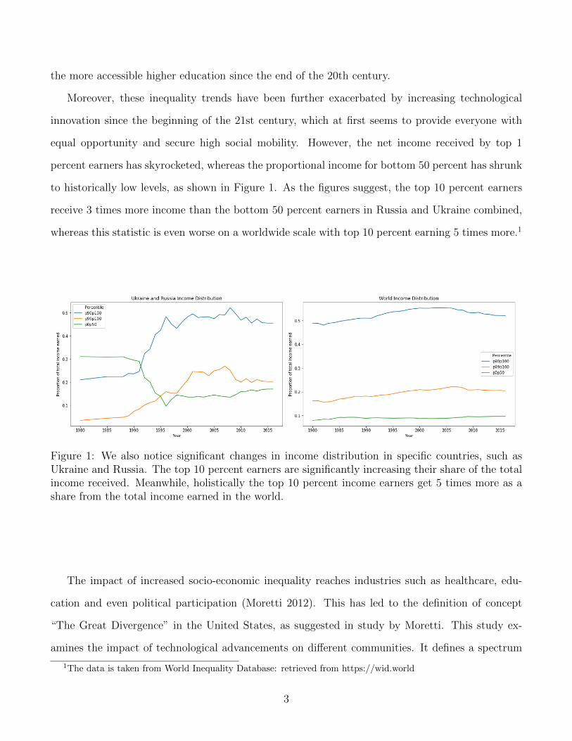
Moreover, these inequality trends have been further exacerbated by increasing technological

innovation since the beginning of the 21st century, which at first seems to provide everyone with

equal opportunity and secure high social mobility. However, the net income received by top 1

percent earners has skyrocketed, whereas the proportional income for bottom 50 percent has shrunk

to historically low levels, as shown in Figure 1. As the figures suggest, the top 10 percent earners

receive 3 times more income than the bottom 50 percent earners in Russia and Ukraine combined,

whereas this statistic is even worse on a worldwide scale with top 10 percent earning 5 times more.1

Figure 1: We also notice significant changes in income distribution in specific countries, such asUkraine and Russia. The top 10 percent earners are significantly increasing their share of the totalincome received. Meanwhile, holistically the top 10 percent income earners get 5 times more as ashare from the total income earned in the world.

The impact of increased socio-economic inequality reaches industries such as healthcare, edu-

cation and even political participation (Moretti 2012). This has led to the definition of concept

“The Great Divergence” in the United States, as suggested in study by Moretti. This study ex-

amines the impact of technological advancements on different communities. It defines a spectrum

1The data is taken from World Inequality Database: retrieved from https://wid.world

3

of cities into three main categories: cities that are adjusting fast to innovation, have high human

capital and are highly investing in research and development (such as San Francisco, San Jose),

cities that are far behind these trends and are failing to incorporate technology into manufacturing

or other industries (such as Flint, Merced), and cities that are somewhere in between. This study’s

key point illustrates that the differences in socio-economic, educational and other fields show no

signs of shrinking. Richer and innovative communities with high proportion of college graduates

are excelling and becoming richer in time, whereas those communities that were already lagging

behind the trends are becoming more incompetitive with obsolete skillsets. These increasing in-

equality leads to huge discrepancies in political participation, nutritional habits and even average

life expectancy.2

Another question in this aspect is what do we mean by defining inequality? The notion of

inequality has both objective and normative features. The former incorporates statistical measures

that capture the variation of tax burden depending on income variation, while the latter has no

empirical or positive economic analysis and is solely based on value judgments and ethical evaluation

(Amartya Sen et al. 1972). Thus, the topic of inequality touches both positive and normative

economic analyses, with the latter being a huge source of debate and disagreement. This paper,

however, analyzes concepts positively and quantitatively, leaving any normative judgments to the

reader.

This paper aims to analyze the relationship between tax progressivity and income inequality,

dig into the phenomenon of flat tax policy that has actively and recently been adopted in numerous

countries. We will utilize the standard notion of inequality as measured by the GINI coefficient

which is calculated from the Lorenz curve of income distribution. As specified in the literature review

later, there are numerous existing progressivity indices, such as Suits or Kakwani idex (1977) and

there are also multiple papers that come up with new measures. However, in this study we will

use a new index as specified in the methodology section of the paper. It is worth to differentiate

2This refers to the book ”The New Geography of Jobs”, Houghton Mifflin Harcourt, 2012, by Enrico Moretti whoexamines the forces of the Great Divergence in America. The book gives holistic view of the economic history, labormarket and the set of new rules that shape today’s technologically driven economy.

4

between two categories of progressivity – structural and effective. Structural progressivity does

not incorporate data about post-taxation income distribution: in other words, it does not measure

how in fact the redistribution happens within the society using the initial (pre-tax) and final (post-

tax) data. Rather it gives a hypothetical measure to the tax system solely based on its income

brackets and tax rates, evaluating the capability of the system to redistribute income. Structural

progressivity ignores what in fact the tax system achieves in the end. On the other hand, effective

progressivity aims to approximate the efficiency of the equitability of the tax system. In ideal case

of no tax evasion and perfect execution of tax rules these two concepts can be used interchangeably.

To refine what other factors rather than tax progressivity we can include later in our model, it

is worth to investigate the time series data of average tax rates. In fact, many papers do not use

complicated progressivity indices and rather opt for average tax rate or top marginal tax rate as

a proxy to measure how progressive is the structure of the existing tax system. A closer look into

the time series reveals that simultaneously with the increase of GINI index, there is a noticeable

trend of decreasing average tax rates for almost all countries. Some of those countries with their

respective average tax rates and GINI indices are shown in Figure 3.

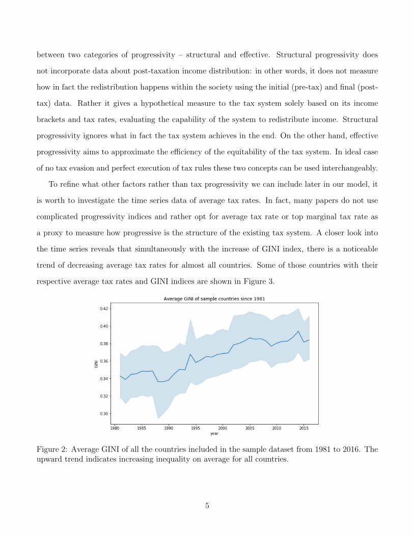
Figure 2: Average GINI of all the countries included in the sample dataset from 1981 to 2016. Theupward trend indicates increasing inequality on average for all countries.

5

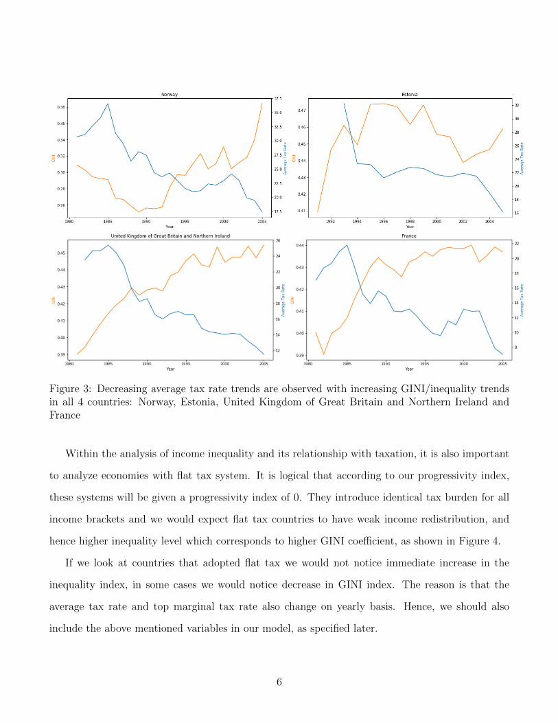
Figure 3: Decreasing average tax rate trends are observed with increasing GINI/inequality trendsin all 4 countries: Norway, Estonia, United Kingdom of Great Britain and Northern Ireland andFrance

Within the analysis of income inequality and its relationship with taxation, it is also important

to analyze economies with flat tax system. It is logical that according to our progressivity index,

these systems will be given a progressivity index of 0. They introduce identical tax burden for all

income brackets and we would expect flat tax countries to have weak income redistribution, and

hence higher inequality level which corresponds to higher GINI coefficient, as shown in Figure 4.

If we look at countries that adopted flat tax we would not notice immediate increase in the

inequality index, in some cases we would notice decrease in GINI index. The reason is that the

average tax rate and top marginal tax rate also change on yearly basis. Hence, we should also

include the above mentioned variables in our model, as specified later.

6

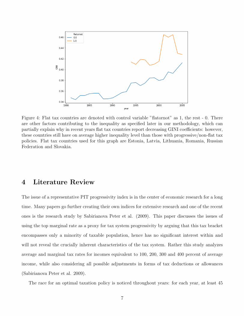
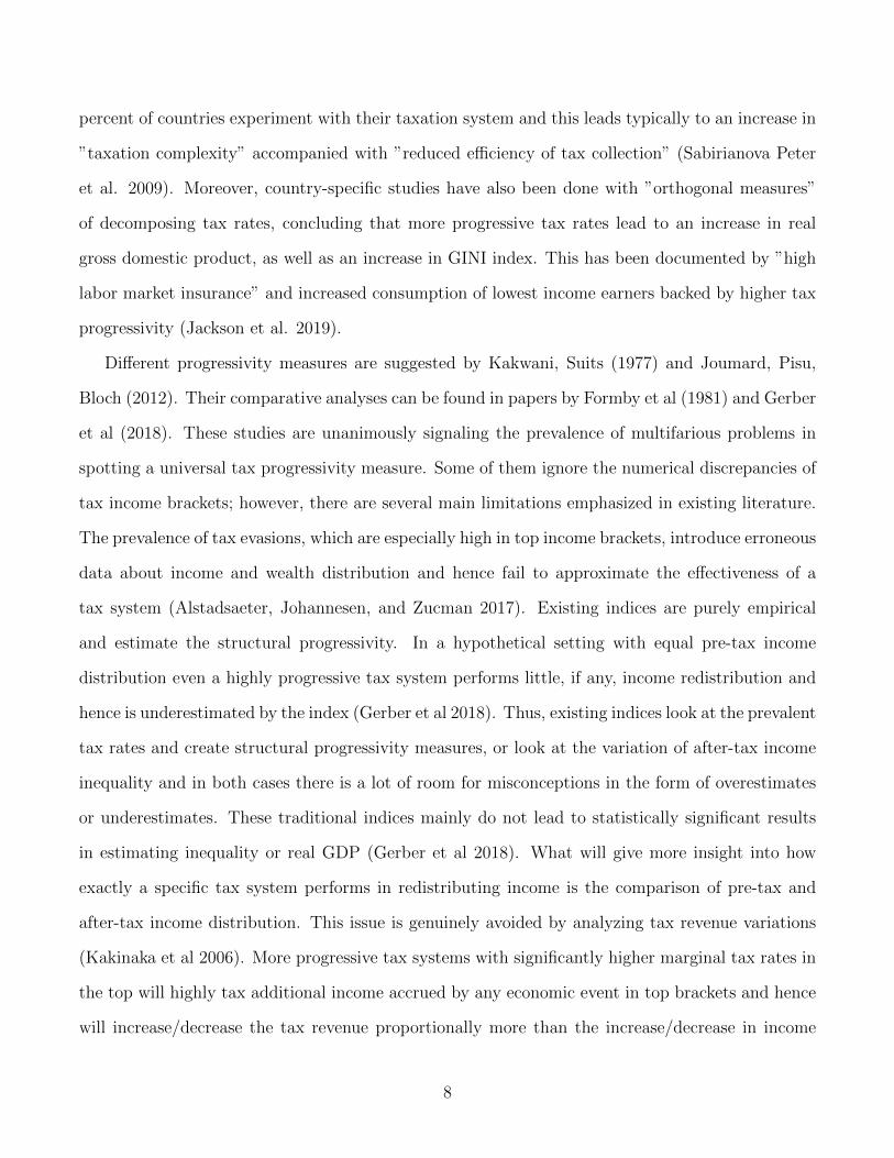
Figure 4: Flat tax countries are denoted with control variable ”flatornot” as 1, the rest - 0. Thereare other factors contributing to the inequality as specified later in our methodology, which canpartially explain why in recent years flat tax countries report decreasing GINI coefficients: however,these countries still have on average higher inequality level than those with progressive/non-flat taxpolicies. Flat tax countries used for this graph are Estonia, Latvia, Lithuania, Romania, RussianFederation and Slovakia.

4 Literature Review

The issue of a representative PIT progressivity index is in the center of economic research for a long

time. Many papers go further creating their own indices for extensive research and one of the recent

ones is the research study by Sabirianova Peter et al. (2009). This paper discusses the issues of

using the top marginal rate as a proxy for tax system progressivity by arguing that this tax bracket

encompasses only a minority of taxable population, hence has no significant interest within and

will not reveal the crucially inherent characteristics of the tax system. Rather this study analyzes

average and marginal tax rates for incomes equivalent to 100, 200, 300 and 400 percent of average

income, while also considering all possible adjustments in forms of tax deductions or allowances

(Sabirianova Peter et al. 2009).

The race for an optimal taxation policy is noticed throughout years: for each year, at least 45

7

percent of countries experiment with their taxation system and this leads typically to an increase in

”taxation complexity” accompanied with ”reduced efficiency of tax collection” (Sabirianova Peter

et al. 2009). Moreover, country-specific studies have also been done with ”orthogonal measures”

of decomposing tax rates, concluding that more progressive tax rates lead to an increase in real

gross domestic product, as well as an increase in GINI index. This has been documented by ”high

labor market insurance” and increased consumption of lowest income earners backed by higher tax

progressivity (Jackson et al. 2019).

Different progressivity measures are suggested by Kakwani, Suits (1977) and Joumard, Pisu,

Bloch (2012). Their comparative analyses can be found in papers by Formby et al (1981) and Gerber

et al (2018). These studies are unanimously signaling the prevalence of multifarious problems in

spotting a universal tax progressivity measure. Some of them ignore the numerical discrepancies of

tax income brackets; however, there are several main limitations emphasized in existing literature.

The prevalence of tax evasions, which are especially high in top income brackets, introduce erroneous

data about income and wealth distribution and hence fail to approximate the effectiveness of a

tax system (Alstadsaeter, Johannesen, and Zucman 2017). Existing indices are purely empirical

and estimate the structural progressivity. In a hypothetical setting with equal pre-tax income

distribution even a highly progressive tax system performs little, if any, income redistribution and

hence is underestimated by the index (Gerber et al 2018). Thus, existing indices look at the prevalent

tax rates and create structural progressivity measures, or look at the variation of after-tax income

inequality and in both cases there is a lot of room for misconceptions in the form of overestimates

or underestimates. These traditional indices mainly do not lead to statistically significant results

in estimating inequality or real GDP (Gerber et al 2018). What will give more insight into how

exactly a specific tax system performs in redistributing income is the comparison of pre-tax and

after-tax income distribution. This issue is genuinely avoided by analyzing tax revenue variations

(Kakinaka et al 2006). More progressive tax systems with significantly higher marginal tax rates in

the top will highly tax additional income accrued by any economic event in top brackets and hence

will increase/decrease the tax revenue proportionally more than the increase/decrease in income

8

that initially led to more/less taxable income (Kakinaka et al 2006). To sum up, Kakinaka’s main

idea in creating a new index is that with progressive systems growth in the tax revenue exceeds the

growth in income. This is unambiguously an effective progressivity measure, because, as opposed

to the structural ones, this index does not use any data about the current tax system, but rather

uses only macroeconomic real-time data and deals with the actual results that the tax system has

achieved. However, the issues of tax avoidance, unreported income and shadow market are still an

issue.

Ever increasing gap between social categories, supported by rising inequality especially observed

since the middle of 20th century (Facundo Alvaredo, Lucas Chancel, Thomas Piketty, Emmanuel

Saez, and Gabriel Zucman, 2005), definitely raise multiple questions of how to combat this inequality

or moderate its consequences, and what is the efficient state of equilibrium in economy. Is inequality

irreversible? Is it good and unavoidable for a growing economy? Many papers have also undertaken

the task to qualitatively tackle this question. However, all existing quantitative approaches have

their drawbacks. What is clear is that the most vulnerable members of the society are earning less

and less income shares each year, while governments are not succeeding in the task of optimally

redistributing income (Thomas Piketty, Emmanuel Saez, Gabriel Zucman, 2018).

5 Data

For this study we need extensive coverage of tax policies, specifically personal income tax indi-

cators that can be further used to construct a new index of progressivity, as well as be used as

a covariate in the linear regression model. The largest available tax database belongs to Andrew

Young School World Tax Indicators, which we will utilize in this study. This dataset covers 189

countries with all income categories and in all regions of the world. This dataset includes variables,

such as average tax rate for income equivalent to 100, 200, 300 and 400 percent of average income,

identical statistics for marginal tax rates, as well as average and marginal tax rate progressivities

(ARPall, ARPmid,MRPall,MRPmid), which correspond to regression coefficients of their respective

9

tax rates regressed on the logarithm of gross income using specific ranges. Even though this statistic

is a good proxy of a country’s structural capacity to redistribute income, we will not use it, because

of several reasons. First, previous studies found no significant relationship between this progres-

sivity measure and inequality. Second, this measure, although uses the logarithm of gross income,

introduces discrepancies between countries that have highly varying income tax brackets. Instead

we will use the marginal tax rates specified in this dataset to construct a new index of structural

tax progressivity. The drawback of this dataset is that it includes data up until the year of 2005.

Data regarding average tax rates from 2000 to 2018 will be taken from OECD tax database, using

the marginal tax rates for income equivalent to 67, 100, 133, 167 percent of average income as set

by central government. OECD dataset covers only 36 countries with no African countries present.

Most of the countries in this dataset are upper-middle or high income countries. Because we need

to include years after 2005 in our analysis, we will study only countries that are covered by both

datasets, total 36 countries all of which are included in OECD tax database. The selection of only

central government tax rates is due to the fact that these tax rates most closely resemble those that

are present in the first dataset. We will also use dataset from the paper by Ligthart and Ji (2012)

to document the countries that have adopted flat tax policy at some point in their history. If in a

specific year, a country adopted flat tax, we will denote a dummy variable with 1, otherwise 0.

Overall, we construct a panel data, where each row corresponds to a specific year, country

with its unique set of variables specified above. We will also add data about the top marginal

tax rates for each country on yearly basis. This corresponds to the marginal tax rate for the

highest income bracket. The original sources for these data are OECD tax database and Michigan

World Tax Database. Note that, from OECD tax database, the data corresponds to column “Top

statutory personal income tax rates” for 2000 - 2018. The data for 1975 – 1999 is from Michigan

World Tax Database. Data for Russia and Ukraine is taken from KPMG individual income tax

table. GINI data for 36 countries will be retrieved from World Inequality Database, as well as real

gross domestic product data from Penn World Tables to account for currency changes and other

confounding factors. Overall, we create a dataset consisting of 38 countries: Australia, Austria,

10

Belgium, Canada, Chile, Czech Republic, Denmark, Estonia, Finland, France, Germany, Greece,

Hungary, Iceland, Ireland, Israel, Italy, Japan, Republic of Korea, Latvia, Lithuania, Luxembourg,

Mexico, Netherlands, New Zealand, Norway, Poland, Portugal, Slovakia, Slovenia, Spain, Sweden,

Switzerland, Turkey, United Kingdom of Great Britain and Northern Ireland, United States of

America, Ukraine, Russian Federation. Overall, our sample consists of 38 countries over 38 years

and equipped with 21 features.

5.1 New Structural Progressivity Index

We will use variables MRy,MR2y,MR3y and MR4y to construct the structural progressivity indices

for each country each year with respect to marginal tax rates.

In order to consider for differences in standard of living and income brackets for different coun-

tries we will not use any nominal variables in any monetary terms, but will rather opt for stan-

dardized approach. Thus, we will denote the α proportion of average income earner as a point on

horizontal axis with x-value equal to alpha. The marginal tax rate applicable to this earner will be

denoted by MRalpha and will be the vertical y value of the point. For each year and each country

we will use linear regression model to fit these points with the following model:

MarginalTaxRateα,r,t= β0 + β1r,t ∗ StandardizedIncomeα,r,t (1)

where r is the index for country, t for year, α is the proportion/multiple of average income,

MarginalTaxRate is the marginal tax rate equivalent to α multiples of the average income earner.

α takes values of 1, 2, 3 and 4 for years 1981-2005 and values 0.67, 1, 1.33 and 1.67 for years

2000-2018.

11

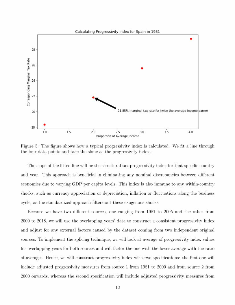
Figure 5: The figure shows how a typical progressivity index is calculated. We fit a line throughthe four data points and take the slope as the progressivity index.

The slope of the fitted line will be the structural tax progressivity index for that specific country

and year. This approach is beneficial in eliminating any nominal discrepancies between different

economies due to varying GDP per capita levels. This index is also immune to any within-country

shocks, such as currency appreciation or depreciation, inflation or fluctuations along the business

cycle, as the standardized approach filters out these exogenous shocks.

Because we have two different sources, one ranging from 1981 to 2005 and the other from

2000 to 2018, we will use the overlapping years’ data to construct a consistent progressivity index

and adjust for any external factors caused by the dataset coming from two independent original

sources. To implement the splicing technique, we will look at average of progressivity index values

for overlapping years for both sources and will factor the one with the lower average with the ratio

of averages. Hence, we will construct progressivity index with two specifications: the first one will

include adjusted progressivity measures from source 1 from 1981 to 2000 and from source 2 from

2000 onwards, whereas the second specification will include adjusted progressivity measures from

12

source 1 from 1981 to 2005 and from source 2 from 2005 onwards.

6 Methodology

The main model is:

GINIt+h,r = α+γh∗Progressivityt,r+θh∗Flatornott,r+δh∗TopRatet,r+σh∗AverageTaxRatet,r+

GINIt−1,r + 1-Year-Lag of Covariates + λr + ηt + εt,r(2)

where h takes values greater than or equal to 0 and is the variable in index used to trace policy

response functions, Progressivityt,r is the index of progressivity, Flatornott,r is the dummy variable

for country r in year t being 1 if the country has flat tax policy enacted in year t and 0 otherwise,

TopRatet,r is the marginal tax rate of the highest income bracket, AverageTaxRatet,r is the avergae

tax rate of average income earner in country r in year t, and the last terms are the 1-year-lags of

the dependent variable and independent variables, country fixed effects, time fixed effects and an

error term. In this study, we will test h values ranging from 0 to 5. Hence, plotting values of θh

with respect to h will show the effect of flat tax policy h years after its implementation. Similar

reasoning holds for other covariates. For example, plotting γh will reveal the response function of

how GINI coefficient is impacted from the Progressivity index prevailing in the economy h years

ago. It is reasonable to expect inverted U-shape response functions for some of these variables due

to time lags of a typical policy.

13

6.1 Why do we include Flatornot

As suggested by Figure 4, flat tax countries have higher inequality. Thus, whether the country

adopted a flat tax system or not can possibly explain the changes in GINI coefficient. In order

to avoid omitted variable bias, the dummy variable for flat tax should be included in the main

model. Moreover, it gives us opportunity to analyze the impact of flat tax policy through response

functions.

6.2 Why do we include AverageTaxRate and TopRate

Figure 6: The relationship between dependent variable GINI and covariate AverageTaxRate.

Figure 6 shows the downward sloping relationship between the average tax rate of an average

income earner and the inequality index (considering also country fixed effects). A higher average

14

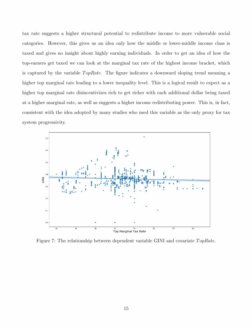
tax rate suggests a higher structural potential to redistribute income to more vulnerable social

categories. However, this gives us an idea only how the middle or lower-middle income class is

taxed and gives no insight about highly earning individuals. In order to get an idea of how the

top-earners get taxed we can look at the marginal tax rate of the highest income bracket, which

is captured by the variable TopRate. The figure indicates a downward sloping trend meaning a

higher top marginal rate leading to a lower inequality level. This is a logical result to expect as a

higher top marginal rate disincentivizes rich to get richer with each additional dollar being taxed

at a higher marginal rate, as well as suggests a higher income redistributing power. This is, in fact,

consistent with the idea adopted by many studies who used this variable as the only proxy for tax

system progressivity.

Figure 7: The relationship between dependent variable GINI and covariate TopRate.

15

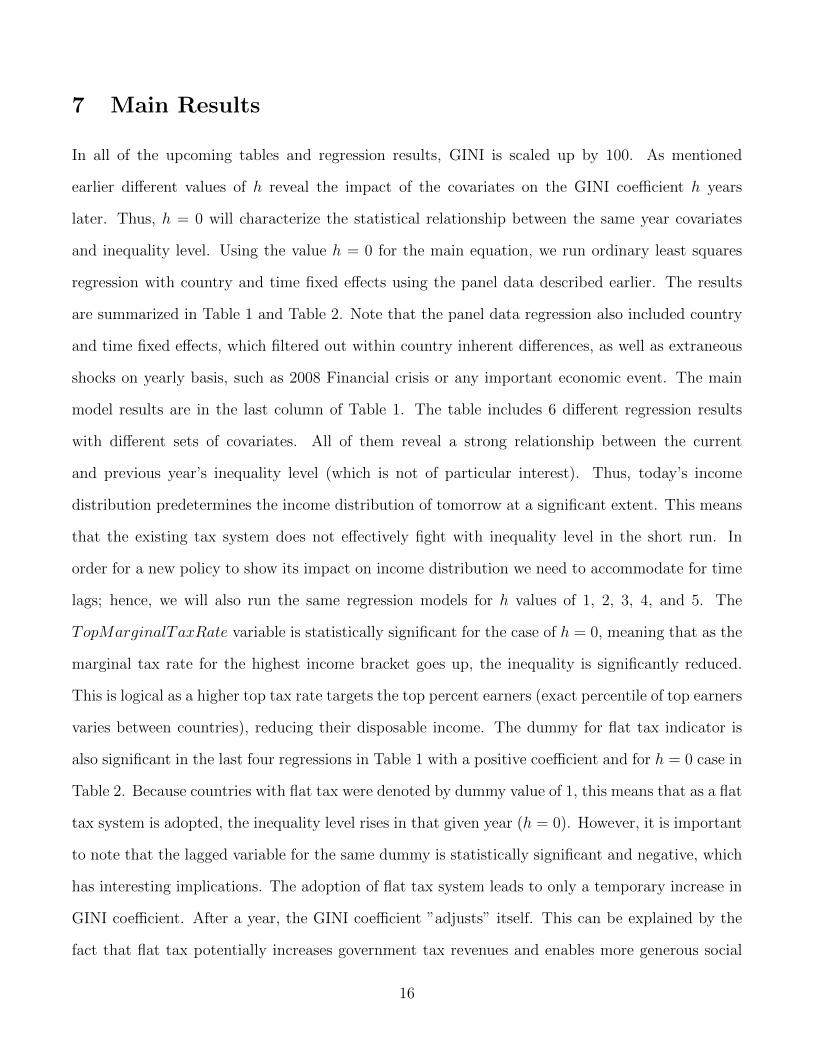
7 Main Results

In all of the upcoming tables and regression results, GINI is scaled up by 100. As mentioned

earlier different values of h reveal the impact of the covariates on the GINI coefficient h years

later. Thus, h = 0 will characterize the statistical relationship between the same year covariates

and inequality level. Using the value h = 0 for the main equation, we run ordinary least squares

regression with country and time fixed effects using the panel data described earlier. The results

are summarized in Table 1 and Table 2. Note that the panel data regression also included country

and time fixed effects, which filtered out within country inherent differences, as well as extraneous

shocks on yearly basis, such as 2008 Financial crisis or any important economic event. The main

model results are in the last column of Table 1. The table includes 6 different regression results

with different sets of covariates. All of them reveal a strong relationship between the current

and previous year’s inequality level (which is not of particular interest). Thus, today’s income

distribution predetermines the income distribution of tomorrow at a significant extent. This means

that the existing tax system does not effectively fight with inequality level in the short run. In

order for a new policy to show its impact on income distribution we need to accommodate for time

lags; hence, we will also run the same regression models for h values of 1, 2, 3, 4, and 5. The

TopMarginalTaxRate variable is statistically significant for the case of h = 0, meaning that as the

marginal tax rate for the highest income bracket goes up, the inequality is significantly reduced.

This is logical as a higher top tax rate targets the top percent earners (exact percentile of top earners

varies between countries), reducing their disposable income. The dummy for flat tax indicator is

also significant in the last four regressions in Table 1 with a positive coefficient and for h = 0 case in

Table 2. Because countries with flat tax were denoted by dummy value of 1, this means that as a flat

tax system is adopted, the inequality level rises in that given year (h = 0). However, it is important

to note that the lagged variable for the same dummy is statistically significant and negative, which

has interesting implications. The adoption of flat tax system leads to only a temporary increase in

GINI coefficient. After a year, the GINI coefficient ”adjusts” itself. This can be explained by the

fact that flat tax potentially increases government tax revenues and enables more generous social

16

assistance programs. The effect of the newly constructed tax progressivity index is not significant

at 90 percent confidence level.

VariablesAverage Tax Rate(for avg. earner)

-0.0151(0.0142)

-0.0124*(6.98e-03)

-0.0117*(6.98e-03)

-0.0111(6.99e-03)

8.05e-03(0.0146)

9.30e-03(0.0149)

Top MarginalTax Rate

-0.0103(9.76e-03)

-3.67e-03(4.80e-03)

-4.35e-03(4.80e-03)

-0.0155*(9.15e-03)

-0.0155*(9.17e-03)

-0.0155*(9.18e-03)

Dummy forFlat tax

-0.322(0.486)

0.252(0.242)

0.773**(0.349)

0.696**(0.353)

0.897**(0.376)

0.905**(0.377)

Progressivityindex 1

-1.59e-03(3.06e-03)

9.70e-04(1.48e-03)

1.04e-03(1.47e-03)

9.97e-04(1.47e-03)

1.07e-03(1.47e-03)

1.86e-03(2.27e-03)

1-year-lagGINI

81.0***(1.82)

80.8***(1.81)

81.0***(1.82)

81.2***(1.85)

81.2***(1.85)

1-year-lagDummy for Flat tax

-0.667**(0.323)

-0.553*(0.333)

-0.638*(0.366)

-0.642*(0.366)

1-year-lagTop Marginal Rate

0.0125(9.01e-03)

0.0130(9.04e-03)

0.0132(9.06e-03)

1-year-lagAverage Tax Rate(for avg. earner)

-0.0208(0.0143)

-0.0221(0.0146)

1-year-lagProgressivity index 1

-1.03e-03(2.27e-03)

Constant34.9***(0.915)

6.78***(0.751)

6.86***(0.750)

6.67***(0.762)

6.42***(0.783)

6.42***(0.784)

Observations 845 820 820 820 812 812R-squared 0.313 0.827 0.828 0.828 0.826 0.826

Table 1: The following table includes 6 different regression model results with different sets ofcovariates. GINI is scaled up by 100. The main model results with all specified covariates includedis in the last column. For this last column, Top Marginal Tax Rate, Dummy for Flat tax, 1-year-lagof Dummy for Flat tax, 1-year-lag of GINI are statistically significant. An interesting case is thesign change of flat tax dummy from current year to the lagged year. *** p < 0.01, ** p < 0.05, *p < 0.1 : Standard errors in parentheses.

17

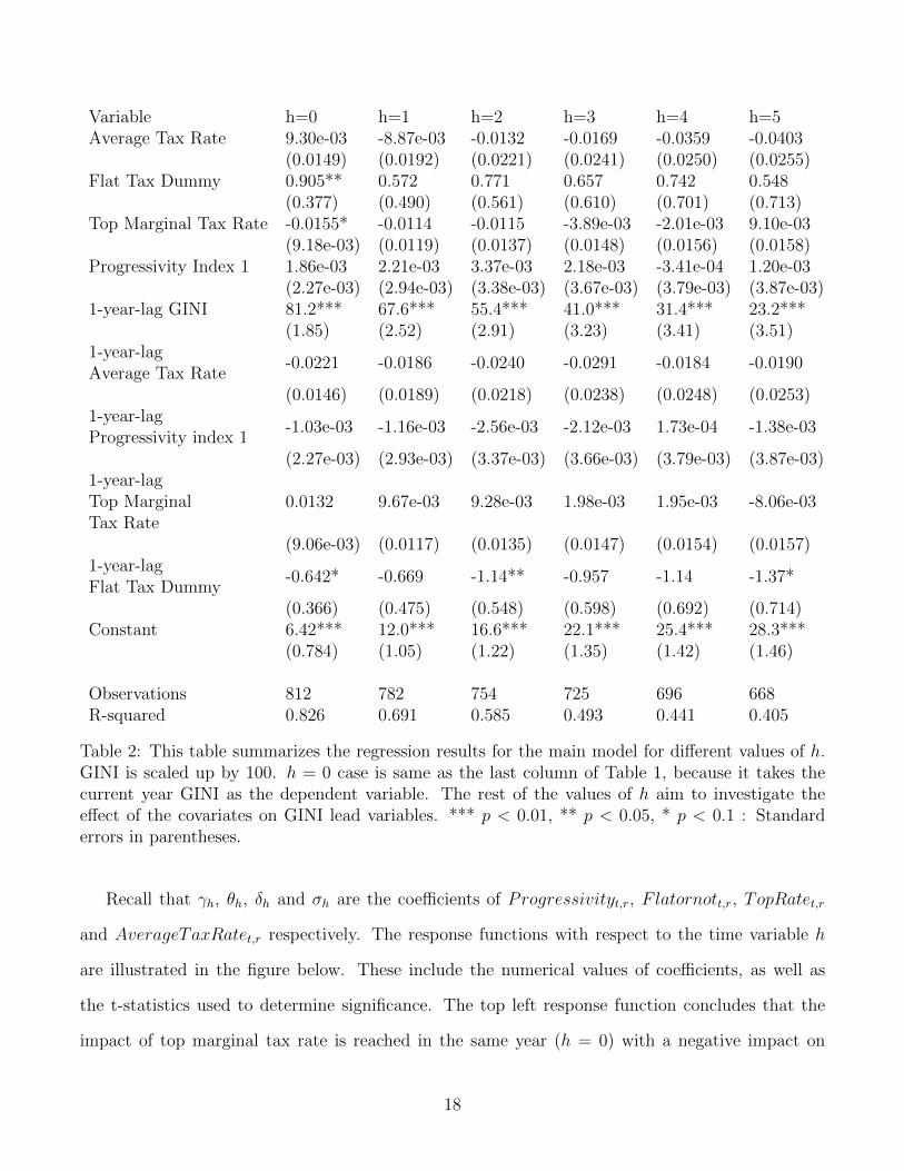
Variable h=0 h=1 h=2 h=3 h=4 h=5Average Tax Rate 9.30e-03 -8.87e-03 -0.0132 -0.0169 -0.0359 -0.0403

(0.0149) (0.0192) (0.0221) (0.0241) (0.0250) (0.0255)Flat Tax Dummy 0.905** 0.572 0.771 0.657 0.742 0.548

(0.377) (0.490) (0.561) (0.610) (0.701) (0.713)Top Marginal Tax Rate -0.0155* -0.0114 -0.0115 -3.89e-03 -2.01e-03 9.10e-03

(9.18e-03) (0.0119) (0.0137) (0.0148) (0.0156) (0.0158)Progressivity Index 1 1.86e-03 2.21e-03 3.37e-03 2.18e-03 -3.41e-04 1.20e-03

(2.27e-03) (2.94e-03) (3.38e-03) (3.67e-03) (3.79e-03) (3.87e-03)1-year-lag GINI 81.2*** 67.6*** 55.4*** 41.0*** 31.4*** 23.2***

(1.85) (2.52) (2.91) (3.23) (3.41) (3.51)1-year-lagAverage Tax Rate

-0.0221 -0.0186 -0.0240 -0.0291 -0.0184 -0.0190

(0.0146) (0.0189) (0.0218) (0.0238) (0.0248) (0.0253)1-year-lagProgressivity index 1

-1.03e-03 -1.16e-03 -2.56e-03 -2.12e-03 1.73e-04 -1.38e-03

(2.27e-03) (2.93e-03) (3.37e-03) (3.66e-03) (3.79e-03) (3.87e-03)1-year-lagTop MarginalTax Rate

0.0132 9.67e-03 9.28e-03 1.98e-03 1.95e-03 -8.06e-03

(9.06e-03) (0.0117) (0.0135) (0.0147) (0.0154) (0.0157)1-year-lagFlat Tax Dummy

-0.642* -0.669 -1.14** -0.957 -1.14 -1.37*

(0.366) (0.475) (0.548) (0.598) (0.692) (0.714)Constant 6.42*** 12.0*** 16.6*** 22.1*** 25.4*** 28.3***

(0.784) (1.05) (1.22) (1.35) (1.42) (1.46)

Observations 812 782 754 725 696 668R-squared 0.826 0.691 0.585 0.493 0.441 0.405

Table 2: This table summarizes the regression results for the main model for different values of h.GINI is scaled up by 100. h = 0 case is same as the last column of Table 1, because it takes thecurrent year GINI as the dependent variable. The rest of the values of h aim to investigate theeffect of the covariates on GINI lead variables. *** p < 0.01, ** p < 0.05, * p < 0.1 : Standarderrors in parentheses.

Recall that γh, θh, δh and σh are the coefficients of Progressivityt,r, Flatornott,r, TopRatet,r

and AverageTaxRatet,r respectively. The response functions with respect to the time variable h

are illustrated in the figure below. These include the numerical values of coefficients, as well as

the t-statistics used to determine significance. The top left response function concludes that the

impact of top marginal tax rate is reached in the same year (h = 0) with a negative impact on

18

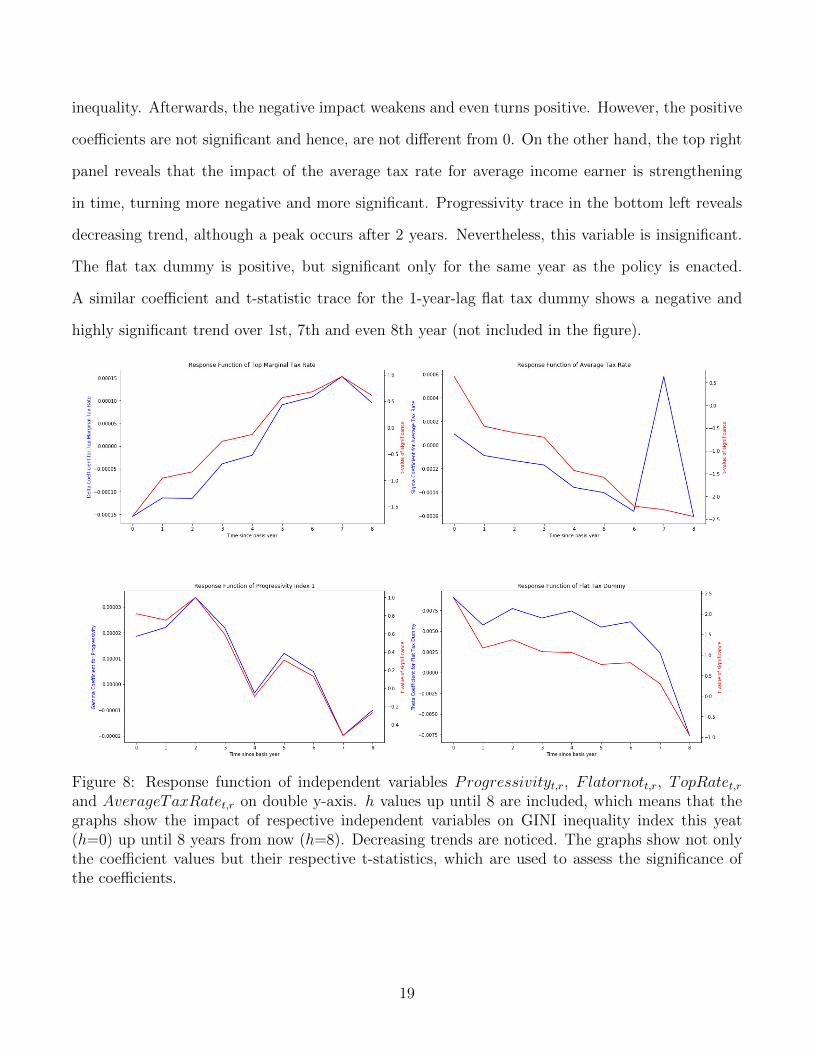
inequality. Afterwards, the negative impact weakens and even turns positive. However, the positive

coefficients are not significant and hence, are not different from 0. On the other hand, the top right

panel reveals that the impact of the average tax rate for average income earner is strengthening

in time, turning more negative and more significant. Progressivity trace in the bottom left reveals

decreasing trend, although a peak occurs after 2 years. Nevertheless, this variable is insignificant.

The flat tax dummy is positive, but significant only for the same year as the policy is enacted.

A similar coefficient and t-statistic trace for the 1-year-lag flat tax dummy shows a negative and

highly significant trend over 1st, 7th and even 8th year (not included in the figure).

Figure 8: Response function of independent variables Progressivityt,r, Flatornott,r, TopRatet,rand AverageTaxRatet,r on double y-axis. h values up until 8 are included, which means that thegraphs show the impact of respective independent variables on GINI inequality index this yeat(h=0) up until 8 years from now (h=8). Decreasing trends are noticed. The graphs show not onlythe coefficient values but their respective t-statistics, which are used to assess the significance ofthe coefficients.

19

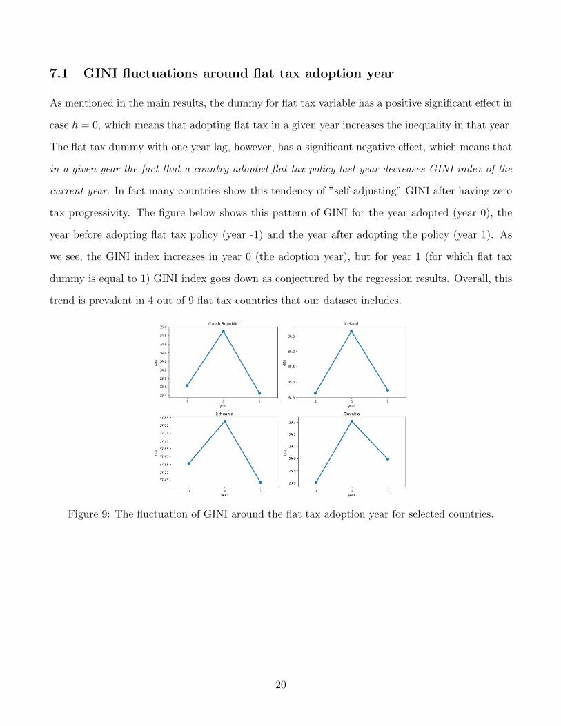
7.1 GINI fluctuations around flat tax adoption year

As mentioned in the main results, the dummy for flat tax variable has a positive significant effect in

case h = 0, which means that adopting flat tax in a given year increases the inequality in that year.

The flat tax dummy with one year lag, however, has a significant negative effect, which means that

in a given year the fact that a country adopted flat tax policy last year decreases GINI index of the

current year. In fact many countries show this tendency of ”self-adjusting” GINI after having zero

tax progressivity. The figure below shows this pattern of GINI for the year adopted (year 0), the

year before adopting flat tax policy (year -1) and the year after adopting the policy (year 1). As

we see, the GINI index increases in year 0 (the adoption year), but for year 1 (for which flat tax

dummy is equal to 1) GINI index goes down as conjectured by the regression results. Overall, this

trend is prevalent in 4 out of 9 flat tax countries that our dataset includes.

Figure 9: The fluctuation of GINI around the flat tax adoption year for selected countries.

20

8 Robustness checks

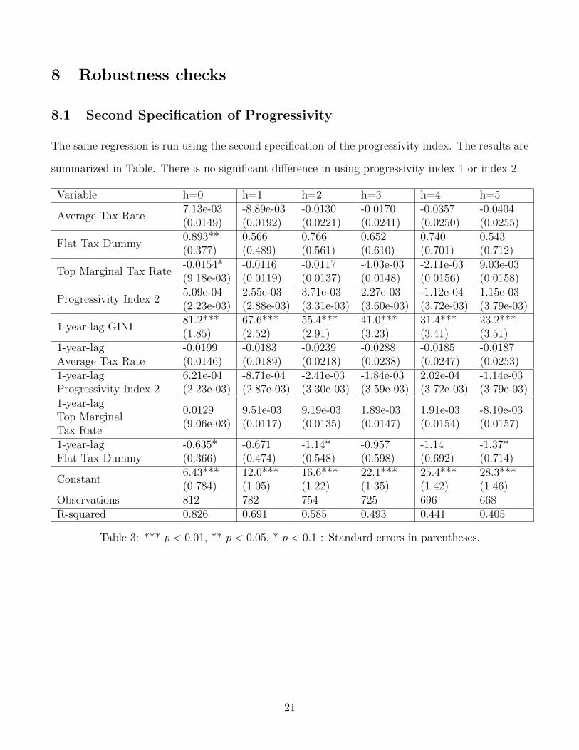
8.1 Second Specification of Progressivity

The same regression is run using the second specification of the progressivity index. The results are

summarized in Table. There is no significant difference in using progressivity index 1 or index 2.

Variable h=0 h=1 h=2 h=3 h=4 h=5

Average Tax Rate7.13e-03(0.0149)

-8.89e-03(0.0192)

-0.0130(0.0221)

-0.0170(0.0241)

-0.0357(0.0250)

-0.0404(0.0255)

Flat Tax Dummy0.893**(0.377)

0.566(0.489)

0.766(0.561)

0.652(0.610)

0.740(0.701)

0.543(0.712)

Top Marginal Tax Rate-0.0154*(9.18e-03)

-0.0116(0.0119)

-0.0117(0.0137)

-4.03e-03(0.0148)

-2.11e-03(0.0156)

9.03e-03(0.0158)

Progressivity Index 25.09e-04(2.23e-03)

2.55e-03(2.88e-03)

3.71e-03(3.31e-03)

2.27e-03(3.60e-03)

-1.12e-04(3.72e-03)

1.15e-03(3.79e-03)

1-year-lag GINI81.2***(1.85)

67.6***(2.52)

55.4***(2.91)

41.0***(3.23)

31.4***(3.41)

23.2***(3.51)

1-year-lagAverage Tax Rate

-0.0199(0.0146)

-0.0183(0.0189)

-0.0239(0.0218)

-0.0288(0.0238)

-0.0185(0.0247)

-0.0187(0.0253)

1-year-lagProgressivity Index 2

6.21e-04(2.23e-03)

-8.71e-04(2.87e-03)

-2.41e-03(3.30e-03)

-1.84e-03(3.59e-03)

2.02e-04(3.72e-03)

-1.14e-03(3.79e-03)

1-year-lagTop MarginalTax Rate

0.0129(9.06e-03)

9.51e-03(0.0117)

9.19e-03(0.0135)

1.89e-03(0.0147)

1.91e-03(0.0154)

-8.10e-03(0.0157)

1-year-lagFlat Tax Dummy

-0.635*(0.366)

-0.671(0.474)

-1.14*(0.548)

-0.957(0.598)

-1.14(0.692)

-1.37*(0.714)

Constant6.43***(0.784)

12.0***(1.05)

16.6***(1.22)

22.1***(1.35)

25.4***(1.42)

28.3***(1.46)

Observations 812 782 754 725 696 668R-squared 0.826 0.691 0.585 0.493 0.441 0.405

Table 3: *** p < 0.01, ** p < 0.05, * p < 0.1 : Standard errors in parentheses.

21

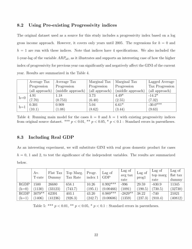
8.2 Using Pre-existing Progressivity indices

The original dataset used as a source for this study includes a progressivity index based on a log

gross income approach. However, it covers only years until 2005. The regressions for h = 0 and

h = 1 are run with these indices. Note that indices have 4 specifications. We also included the

1-year-lag of the variable ARPall, as it illustrates and supports an interesting case of how the higher

index of progressivity for previous year can significantly and negatively affect the GINI of the current

year. Results are summarized in the Table 4.

Average TaxProgression(all approach)

Average TaxProgression(middle approach)

Marginal TaxProgression(all approach)

Marginal TaxProgression(middle approach)

Lagged AverageTax Progression(all approach)

h=04.91(7.70)

1.18(0.753)

3.73(6.40)

4.49*(2.55)

-14.2*(7.32)

h=10.301(10.1)

0.909(1.08)

5.04(8.62)

6.61*(3.44)

-30.0***(9.63)

Table 4: Running main model for the cases h = 0 and h = 1 with existing progressivity indicesfrom original source dataset. *** p < 0.01, ** p < 0.05, * p < 0.1 : Standard errors in parentheses.

8.3 Including Real GDP

As an interesting experiment, we will substitute GINI with real gross domestic product for cases

h = 0, 1 and 2, to test the significance of the independent variables. The results are summarized

below.

Av.T-rate

Flat TaxDummy

Top Marg.Tax Rate

Progr.index 1

Lag ofGDP

Lag ofavg taxrate

Lag ofprog1

Lag oftop margrate

Lag offlat taxdummy

RGDP(h=0)

1500(1130)

26680(33123)

658.1(743.7)

10.26(195.1)

0.992***(0.00466)

-996(1091)

29.59(190.5)

-830.9(730.5)

11345(32730)

RGDP(h=1)

3079**(1406)

62391(41236)

403.1(926.3)

43.20(242.7)

0.989***(0.00606)

-2829**(1359)

38.22(237.3)

-740(910.4)

21021(40812)

Table 5: *** p < 0.01, ** p < 0.05, * p < 0.1 : Standard errors in parentheses.

22

9 Conclusion and Discussion

The insignificance of progressivity index in the model signals that there is no statistically significant

difference in inequality levels based on how ”progressive” the tax system is. In other words, as long as

the tax system is progressive, the tax system will not significantly increase or decrease the inequality

level, and hence, is an inefficient tool to affect GINI index. This result is solely based on the index

we created, as well as several other indices used in the robustness checks section of this paper.

However, the main model revealed an interesting implication of flat tax policy we did not intend

to discover in the initial stages of developing this paper. As the country switches from progressive

system to a flat tax system, its inequality level measured by GINI index is significantly increased,

emphasizing that the main beneficiaries of the flat tax policy are the top earners, who enjoy higher

disposable incomes after the policy. Yet, this effect is completely reversed in 4 of the 9 flat tax

countries analyzed, with lagged dummy flat tax variable yielding negative significant coefficients

for almost all values of h in the main model (see Table 2). This opens an interesting discussion of

whether the equilibrium inequality level in the economy is ”self-adjusting” in time or has a long-run

equilibrium level to which it converges with the flat tax policy being the process through which it

reaches certain level of inequality rather than the reason. Do certain countries benefit from flat

tax depending on where they are located on income spectrum or the general state of the economic

development (why mostly Eastern European countries are adopting flat tax policies)? A conjecture

might be that flat tax policy increases the tax revenues for a government a year after and enables a

more generous package of social assistance similar to the trickle-up economics argument by Jackson

et al. (2019).

10 Departing Notes

This paper showed that progressive systems have the same power to combat inequality, regardless of

their measure of progressivity. A truly equitable society has not been achieved in practice. This and

many already existing papers could not establish taxation as an effective method for significantly

23

affecting income distribution; taxation can be thought of as a lost tool to fight inequality. The

realms of economic and social inequality have long been rooted and grown into so many aspects of

life that thinking about inequality through a GINI coefficient is a naive idea. Our view of inequality

ignores the opportunities available to people and the presence of these opportunities conditioned

by economic inequality, location, demography and else. The notion of inequality needs to reflect

the social complexity we are living in.

11 References

1 Alstadsæter, A., Niels Johannesen, and Gabriel Zucman. ”Tax evasion and inequality (No.

w23772).” National Bureau of Economic Research, www. nber. org/papers/w23772, accessed

April 1 (2017): 2018.

2 Alvaredo, Facundo, Lucas Chancel, Thomas Piketty, Emmanuel Saez, and Gabriel Zucman. 2017.

”Global Inequality Dynamics: New Findings from WID.world.” American Economic Review,

107 (5): 404-09.

3 Bourguignon, Francois. ”Revisiting the Debate on Inequality and Economic Development”, Re-

vue d’economie politique, vol. vol. 125, no. 5, 2015, pp. 633-663.

4 DeLong, J. Bradford. ”A Brief History of Modern Inequality.” World Economic Forum. Vol. 28.

2016.

24

5 Formby, John P., Terry G. Seaks, and W. James Smith. ”A comparison of two new measures of

tax progressivity.” The Economic Journal 91.364 (1981): 1015-1019.

6 Gerber, Claudia, et al. Personal income tax progressivity: trends and implications. International

Monetary Fund, 2018.

7 Jackson, Laura E., Christopher Otrok, and Michael T. Owyang. Tax Progressivity, Economic

Booms, and Trickle-Up Economics. No. 2019-34. 2019.

8 Joumard, Isabelle, Mauro Pisu, and Debra Bloch. ”Less income inequality and more growth–are

they compatible? Part 3. Income redistribution via taxes and transfers across OECD coun-

tries.” (2012). APA

9 Ji, Kan and Jenny E. Ligthart. “The Causes and Consequences of the Flat Income Tax.” (2012).

10 Kakinaka, Makoto, and Rodrigo M. Pereira. ”A new measurement of tax progressivity.” In-

ternational University of Japan, Graduate School of International Relations Working Paper

EDP06-7 (2006).

11 Kuznets, Simon. ”Economic growth and income inequality.” The American economic review

45.1 (1955): 1-28.

12 Moretti, Enrico. The new geography of jobs. Houghton Mifflin Harcourt, 2012.

25

13 Piketty, Thomas, Emmanuel Saez, and Gabriel Zucman. ”Distributional national accounts:

methods and estimates for the United States.” The Quarterly Journal of Economics 133.2

(2018): 553-609.

14 Sabirianova Peter, Klara, Steve Buttrick, and Denvil Duncan. ”Global reform of personal

income taxation, 1981-2005: Evidence from 189 countries.” Andrew Young School of Policy

Studies Research Paper Series 08-08 (2009). APA

15 Sen, Amartya, et al. On economic inequality. Oxford University Press, 1997.

16 Slemrod, Joel. ”Taxation and inequality: a time-exposure perspective.” Tax policy and the

economy 6 (1992): 105-127.

26