Analyzing the Income Distribution in Hawaii

August 2021 Department of Business, Economic Development & Tourism Research and Economic Analysis Division

This report is prepared by Dr. Wayne Liou, Economist, under the direction of Dr. Eugene Tian, Division Administrator. Dr. Joseph Roos, Economic Research Program Manager, reviewed the report and provided valuable recommendations.

Table of Contents I. Introduction ............................................................................................................................. 4

II. Data and Methodology ......................................................................................................... 5

III. Income Distribution in Hawaii............................................................................................. 6

IV. Household and Housing Characteristics by Household Income Quintiles .......................... 7

V. Annual Household Income Source Breakdown ................................................................. 15

VI. Individual Characteristics by Individual Income Quintiles ............................................... 16

VII. Conclusion ......................................................................................................................... 23

4 | P a g e

I. Introduction Within the past few years, there has been increased attention paid to evaluating income distribution and the effects of growing income inequality. Work by Piketty1 and Saez and Zucman2 are usually pointed to as bringing rather technical analyses of income distribution and inequality into the mainstream; Piketty’s Capital in the Twenty-First Century, for example, was a New York Times #1 Bestseller and spawned a Netflix documentary. Case and Deaton3 coined the (now) commonly used term “deaths of despair,” pointing to the association between rising inequality and increased suffering among the working class that has led to a growth in deaths by drugs, alcohol, and suicide. From a macro standpoint, international organizations like the International Monetary Fund (IMF)4 and Organization for Economic Cooperation and Development (OECD)5 have analyzed how income inequality can negatively affect economic growth. Looking beyond academia, recent protests highlight concerns about how income inequality is affecting social fabric. (That being said, some income inequality is unavoidable – e.g. younger workers with less experience earning less than older, more experienced workers – and can be good for economic growth by providing incentives to be productive6).

This report looks to initiate a closer look at income inequality in Hawaii by considering the different characteristics of households and individuals across the income distribution. As an initial baseline analysis, this report is intended to serve as making note of factors that can contribute to household or individual income inequality without delving too deeply into a complex model of how a particular characteristic contributes to a particular amount of inequality. Accordingly, the primary analysis of this report is dividing households and workers into income quintiles and comparing characteristics of households and workers across quintiles. This report does not explore the role that income mobility plays in the socioeconomic wellbeing of the community, in part due to the difficulty in tracking one’s income across multiple years.

There are at least two other written products that provide a closer look at income inequality in Hawaii. Recently, the Economic Research Organization at the University of Hawaii (UHERO) posted a blog in 2014 looking at income inequality in Hawaii since the 1950s using IRS and

1 Piketty, T. (2014). Capital in the Twenty-First Century. Harvard University Press. 2 Saez, E. and Zucman, G. (2016). Wealth Inequality in the United States Since 1913: Evidence from Capitalized Income Tax Data. Quarterly Journal of Economics, 131(2): 519-578. Also, Picketty, T., Saez, E., and Zucman, G. (2018). Distributional National Accounts: Methods and Estimates for the United States. Quarterly Journal of Economics, 133(2): 553-609. 3 Case, A. and Deaton, A. (2017). Mortality and Morbidity in the 21st Century. Brookings Papers on Economic Activity. 4 Aiyar, S. and Ebeke, C. (2019). Inequality of Opportunity, Inequality of Income and Economic Growth. IMF Working Paper 19/34. Available at https://www.imf.org/en/Publications/WP/Issues/2019/02/15/Inequality-of-Opportunity-Inequality-of-Income-and-Economic-Growth-46566. 5 Cingano, F. (2014). Trends in Income Inequality and its Impact on Economic Growth. OECD Social, Employment and Migration Working Papers, No. 163. Available at https://www.oecd-ilibrary.org/social-issues-migration-health/trends-in-income-inequality-and-its-impact-on-economic-growth_5jxrjncwxv6j-en. 6 Grigoli, F. (2017). “A New Twist on the Link Between Inequality and Economic Development.” IMF Blog. Available at https://blogs.imf.org/2017/05/11/a-new-twist-in-the-link-between-inequality-and-economic-development/.

5 | P a g e

Hawaii Department of Taxation data7. Another product is a 2007 report from the East-West Center by Dr. Seiji Naya, looking at the income distribution of Native Hawaiians in particular. This East-West Center report examines income distribution and its relation to poverty, highlighting the high poverty rates among Native Hawaiians8.

II. Data and Methodology There are a couple of common ways to evaluate a population’s income distribution. Perhaps the most common way is via the Gini coefficient. The basic idea of the Gini coefficient is to measure how differently income is distributed relative to a society where everyone earns the same income and income is distributed evenly. The Lorenz Curve is a graphical representation of income inequality, plotting the cumulative share of the population’s income or wealth on the vertical axis with the percentiles of the population along the horizontal axis. A population with zero income inequality (everyone earns the same amount) will have a Lorenz Curve that is a line at 45 degrees; a population with total income inequality (one person earns the entire population’s income and everyone else earns $0) will have a Lorenz Curve that is a flat line along the x-axis until the 100th percentile, where the curve jumps up to the 100% cumulative income mark. The area between a population’s Lorenz Curve and the 45 degree line is the Gini coefficient. A Gini coefficient of zero means there is no area between the Lorenz Curve and the 45 degree line, meaning there is no income inequality. A Gini coefficient of 1 means there is complete income inequality, as the Lorenz curve’s flatness along the x-axis until the 100th percentile leads to the area between the 45 degree line and the Lorenz Curve being the totality of the area under the 45 degree line.

A second summary measure of income distribution is the Kuznets Ratio. This is the ratio of income received by the top 20% of the population to the income received by the bottom 40% of the population. A higher ratio indicates that more income is earned by the richer income groups. This measure is easier to calculate than the Gini coefficient, and ties with the next method of analyzing income distribution.

This report focuses its analysis of income distribution by separating households into quintiles based on household income. This follows conventional income distribution analyses as conducted by researchers like those at the U.S. Census Bureau9, U.S. Bureau of Economic Analysis10, and U.S. Congressional Budget Office11. Comparing the average income within each quintile provides additional insight into how much the poorest households are earning relative to

7 Page, J. and Halliday, T. (2014). Income Inequality in Hawaii Since Statehood. Available at https://uhero.hawaii.edu/income-inequality-in-hawaii-since-statehood/. 8 Naya, S. (2007). Income Distribution and Poverty Alleviation for the Native Hawaiian Community. East-West Center Working Papers, Economic Series, No. 91. Available at https://www.eastwestcenter.org/publications/income-distribution-and-poverty-alleviation-native-hawaiian-community. 9 Current Population Survey Tables for Household Income, Table HINC-05, “Percent Distribution of Households, by Selected Characteristics Within Income Quintile and Top 5 Percent,” available at https://www.census.gov/data/tables/time-series/demo/income-poverty/cps-hinc/hinc-05.html. 10 Distribution of Personal Income, available at https://www.bea.gov/data/special-topics/distribution-of-personal-income. Note that the tables include income distribution by deciles, among other percentiles. 11 Reports by the U.S. Congressional Budget Office on income distribution are available at https://www.cbo.gov/topics/income-distribution.

6 | P a g e

the richest, and approximately what the median household income of the population is. An additional benefit to dividing the population into income quintiles is that characteristics of households and individuals within each quintile can be analyzed, providing closer insight into what factors could affect or are affected by income. To provide additional context to the current state of the income distribution in Hawaii, historical measures of income distribution in the U.S. and Hawaii are included.

To analyze the different income quintiles, this report relies on data from the American Community Survey (ACS), using the most recent ACS 5-year sample available, 2015-2019. The main unit of analysis with respect to income is the household, as it is generally at the household level that decisions about whether to work and earn income or stay at home and focus on household production, or to have a roommate or tenant to help with housing costs. With that being said, certain demographics and socioeconomic characteristics are more correlated to an individual’s income – an individual’s educational attainment is going to be more closely aligned with the individual’s own personal income, though it will likely be correlated to a spouse’s education (and thus the spouse’s and household income). To address these factors, a brief analysis of individual income distribution will be done in this report. (Using the individual as a unit of analysis will also allow analysis of individuals living in group quarters).

III. Income Distribution in Hawaii The Gini coefficient and Kuznets Ratio for Hawaii and the U.S. are provided in the table below (Table 1). The income distribution is evolving to a more unequal distribution, with both Gini coefficient and Kuznets ratio generally growing in the U.S. and in Hawaii. These measures point to less income inequality in Hawaii relative to the nation.

Table 1. Income Inequality in Hawaii and the U.S., by Household Income, 2010-2019

Year Gini coefficient Kuznets Ratio

Hawaii U.S. Hawaii U.S. 2019 0.440 0.481 3.61 4.43 2018 0.445 0.485 3.74 4.53 2017 0.446 0.482 3.77 4.48 2016 0.442 0.482 3.68 4.49 2015 0.435 0.482 3.52 4.46 2014 0.433 0.480 3.48 4.46 2013 0.440 0.481 3.63 4.47 2012 0.426 0.476 3.41 4.36 2011 0.430 0.475 3.45 4.35 2010 0.433 0.469 3.51 4.23

Source: U.S. Census Bureau tables, B19083: Gini Index of Income Inequality, and B19082: Shares of Aggregate Household Income by Quintile. American Community Survey, 1-year sample. Available at https://data.census.gov/cedsci/.

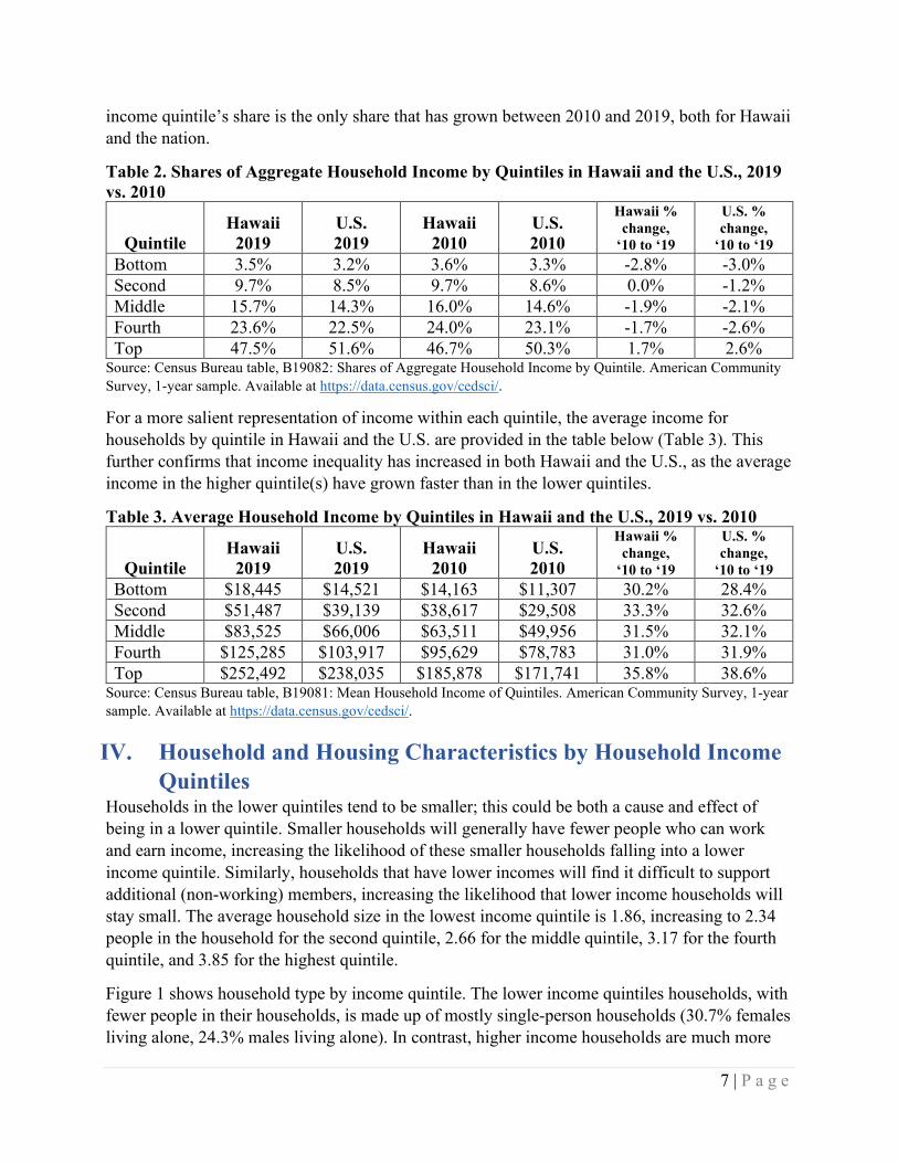
The share of total household income received by each income quintile (which factors into the calculation of the Kuzents Ratio) is in Table 2. Hawaii has a higher share of income in the lower income quintiles relative to the U.S., pointing to less income inequality in Hawaii. The top

7 | P a g e

income quintile’s share is the only share that has grown between 2010 and 2019, both for Hawaii and the nation.

Table 2. Shares of Aggregate Household Income by Quintiles in Hawaii and the U.S., 2019 vs. 2010

Quintile Hawaii

2019 U.S. 2019

Hawaii 2010

U.S. 2010

Hawaii % change,

‘10 to ‘19

U.S. % change,

‘10 to ‘19 Bottom 3.5% 3.2% 3.6% 3.3% -2.8% -3.0% Second 9.7% 8.5% 9.7% 8.6% 0.0% -1.2% Middle 15.7% 14.3% 16.0% 14.6% -1.9% -2.1% Fourth 23.6% 22.5% 24.0% 23.1% -1.7% -2.6% Top 47.5% 51.6% 46.7% 50.3% 1.7% 2.6%

Source: Census Bureau table, B19082: Shares of Aggregate Household Income by Quintile. American Community Survey, 1-year sample. Available at https://data.census.gov/cedsci/.

For a more salient representation of income within each quintile, the average income for households by quintile in Hawaii and the U.S. are provided in the table below (Table 3). This further confirms that income inequality has increased in both Hawaii and the U.S., as the average income in the higher quintile(s) have grown faster than in the lower quintiles.

Table 3. Average Household Income by Quintiles in Hawaii and the U.S., 2019 vs. 2010

Quintile Hawaii

2019 U.S. 2019

Hawaii 2010

U.S. 2010

Hawaii % change,

‘10 to ‘19

U.S. % change,

‘10 to ‘19 Bottom $18,445 $14,521 $14,163 $11,307 30.2% 28.4% Second $51,487 $39,139 $38,617 $29,508 33.3% 32.6% Middle $83,525 $66,006 $63,511 $49,956 31.5% 32.1% Fourth $125,285 $103,917 $95,629 $78,783 31.0% 31.9% Top $252,492 $238,035 $185,878 $171,741 35.8% 38.6%

Source: Census Bureau table, B19081: Mean Household Income of Quintiles. American Community Survey, 1-year sample. Available at https://data.census.gov/cedsci/.

IV. Household and Housing Characteristics by Household Income Quintiles

Households in the lower quintiles tend to be smaller; this could be both a cause and effect of being in a lower quintile. Smaller households will generally have fewer people who can work and earn income, increasing the likelihood of these smaller households falling into a lower income quintile. Similarly, households that have lower incomes will find it difficult to support additional (non-working) members, increasing the likelihood that lower income households will stay small. The average household size in the lowest income quintile is 1.86, increasing to 2.34 people in the household for the second quintile, 2.66 for the middle quintile, 3.17 for the fourth quintile, and 3.85 for the highest quintile.

Figure 1 shows household type by income quintile. The lower income quintiles households, with fewer people in their households, is made up of mostly single-person households (30.7% females living alone, 24.3% males living alone). In contrast, higher income households are much more

8 | P a g e

likely to be married, both with children and without children (27.0% and 48.6%, respectively, for the top quintile). The latter could still have other relatives (parents, siblings, or in-laws) and non-relatives in the household, so an average household size of significantly more than two people among these higher income quintiles is not unreasonable. Childless households where a spouse or partner or not present, but another relative is, are prevalent in relatively stable numbers across the income quintiles.

Figure 1. Household Type by Household Income Quintile

Source: American Community Survey, 2015-2019 5-year sample.

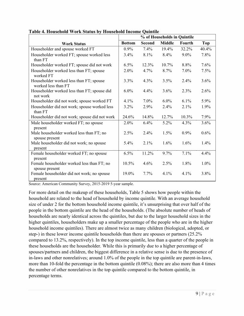
Table 4 shows the work status of the household as a percentage within each income quintile. Higher income quintiles are far more likely to have a householder and spouse working, with over 40% of households in the top quintile having both householder and spouse working full time. In contrast, in almost a quarter of households in the bottom quintile, neither householder nor spouse is working at all; in almost 30% of households in the bottom quintile, a female householder with no spouse present is working less than full time.

7.4%15.5%

19.9%26.3% 27.0%14.7%

24.5%

34.7%

40.6%48.6%

2.2%

3.5%

4.8%

4.8%

3.8%

30.7%

16.7%

9.4%

3.4%

2.4%

7.6%4.5%

2.6%1.6%

6.0%8.6%

7.0%7.4%

6.1%24.3% 16.3%

11.0%5.9% 3.0%

2.6% 3.6% 3.3% 3.6% 3.2%

0

10000

20000

30000

40000

50000

60000

70000

80000

90000

100000

Bottom Second Middle Fourth Top

Num

ber o

f hou

seho

lds

Male householder, no spouse/partner present,only nonrelatives present

Male householder, no spouse/partner present,with relatives, no children of the householderless than 18Male householder, no spouse/partner present,with children of the householder less than 18

Male householder, no spouse/partner present,living alone

Female householder, no spouse/partnerpresent, only nonrelatives present

Female householder, no spouse/partnerpresent, with relatives, no children of thehouseholder less than 18Female householder, no spouse/partnerpresent, with children of the householder lessthan 18Female householder, no spouse/partnerpresent, living alone

Cohabiting couple household, no children of thehouseholder less than 18

Cohabiting couple household with children ofthe householder less than 18

Married couple household, no children of thehouseholder less than 18

Married couple household with children of thehouseholder less than 18

9 | P a g e

Table 4. Household Work Status by Household Income Quintile

Work Status % of Households in Quintile

Bottom Second Middle Fourth Top Householder and spouse worked FT 0.9% 7.4% 19.4% 32.2% 40.4% Householder worked FT; spouse worked less

than FT 3.4% 8.1% 8.4% 9.0% 7.8%

Householder worked FT; spouse did not work 6.5% 12.3% 10.7% 8.8% 7.6% Householder worked less than FT; spouse

worked FT 2.0% 4.7% 8.7% 7.0% 7.5%

Householder worked less than FT; spouse worked less than FT

3.3% 4.3% 3.5% 2.4% 3.6%

Householder worked less than FT; spouse did not work

6.0% 4.4% 3.6% 2.3% 2.6%

Householder did not work; spouse worked FT 4.1% 7.0% 6.0% 6.1% 5.9% Householder did not work; spouse worked less

than FT 3.2% 2.9% 2.4% 2.1% 1.9%

Householder did not work; spouse did not work 24.6% 14.8% 12.7% 10.3% 7.9% Male householder worked FT; no spouse

present 2.0% 6.4% 5.2% 4.3% 3.6%

Male householder worked less than FT; no spouse present

2.5% 2.4% 1.5% 0.9% 0.6%

Male householder did not work; no spouse present

5.4% 2.1% 1.6% 1.6% 1.4%

Female householder worked FT; no spouse present

6.5% 11.2% 9.7% 7.1% 4.4%

Female householder worked less than FT; no spouse present

10.5% 4.6% 2.5% 1.8% 1.0%

Female householder did not work; no spouse present

19.0% 7.7% 4.1% 4.1% 3.8%

Source: American Community Survey, 2015-2019 5-year sample.

For more detail on the makeup of these households, Table 5 shows how people within the household are related to the head of household by income quintile. With an average household size of under 2 for the bottom household income quintile, it’s unsurprising that over half of the people in the bottom quintile are the head of the households. (The absolute number of heads of households are nearly identical across the quintiles, but due to the larger household sizes in the higher quintiles, householders make up a smaller percentage of the people who are in the higher household income quintiles). There are almost twice as many children (biological, adopted, or step-) in these lower income quintile households than there are spouses or partners (25.2% compared to 13.2%, respectively). In the top income quintile, less than a quarter of the people in these households are the householder. While this is primarily due to a higher percentage of spouses/partners and children, the biggest difference in a relative sense is due to the presence of in-laws and other nonrelatives; around 1.0% of the people in the top quintile are parent-in-laws, more than 10-fold the percentage in the bottom quintile (0.08%); there are also more than 4 times the number of other nonrelatives in the top quintile compared to the bottom quintile, in percentage terms.

10 | P a g e

Table 5. Relationships to Household Head by Household Income Quintile

Relationship to Household Head % of Households in Quintile

Bottom Second Middle Fourth Top Head of household 51.7% 40.1% 35.5% 28.9% 23.2% Opposite-sex husband/wife/spouse 11.4% 15.9% 18.9% 19.2% 17.4% Opposite-sex unmarried partner 1.8% 2.2% 2.5% 1.8% 1.1% Same-sex husband/wife/spouse 0.1% 0.1% 0.3% 0.2% 0.2% Same-sex unmarried partner 0.1% 0.1% 0.2% 0.2% 0.1% Biological son or daughter 23.9% 26.2% 26.6% 28.7% 27.1% Adopted son or daughter 0.7% 0.5% 0.7% 0.7% 0.6% Stepson or stepdaughter 0.5% 0.9% 0.8% 0.9% 1.0% Brother or sister 1.3% 1.7% 1.7% 1.9% 2.7% Father or mother 1.5% 2.0% 1.9% 2.2% 2.6% Grandchild 2.5% 3.5% 3.3% 5.0% 6.5% Parent-in-law 0.08% 0.3% 0.4% 0.6% 1.0% Son-in-law or daughter-in-law 0.3% 0.6% 0.9% 1.7% 2.8% Other relative 1.3% 2.3% 2.4% 3.1% 5.7% Roommate or housemate 1.4% 1.6% 1.7% 2.2% 2.4% Foster child 0.1% 0.1% 0.1% 0.0% 0.1% Other nonrelative 1.3% 2.0% 2.0% 2.7% 5.5%

Source: American Community Survey, 2015-2019 5-year sample.

Figure 2 and Figure 3 present the gender and age of the head of household. Lower income quintiles are headed by females at a higher rate compared to higher income quintiles. Even though culturally it’s more likely for the head of household to be male, in the bottom household income quintile, a female is the head of household 56.2% of the time; for the other quintiles, the majority of householders are male. In the top income quintile, 10.3% of householders are single females and 8.8% of householders are single males (see Figure 1), meaning that just over 40% of married and cohabiting couples in the top quintile have female heads of households. This percentage is about the same for the bottom income quintile and slightly higher for the middle and fourth quintile (about 43% and 42%, respectively).

11 | P a g e

Figure 2. Gender of Householder by Household Income Quintile

Source: American Community Survey, 2015-2019 5-year sample.

The bottom couple of quintiles are relatively more likely to be older than 65 and younger than 25. This could point to both older households where the householder is retired and not earning labor income and younger households that are still in school, earning minimal labor income. The middle few quintiles are more likely to have householders between the age of 26 and 45, adults who are more likely to be working full time, but perhaps still limited in their income sources – peak career earnings tend to happen later in life, and there has not been as much time to accumulate assets that provide additional income (e.g., stock market and real estate investments).

Figure 3. Age of Householder by Household Income Quintile

Source: American Community Survey, 2015-2019 5-year sample.

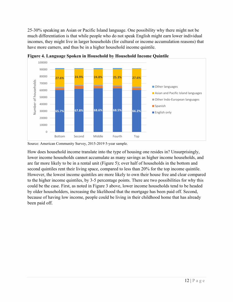
The language spoken in the household does not differentiate much across the different income quintiles (Figure 4). Around 65-70% of households within each quintile speak English only, with

43.8%51.1% 52.6% 55.3% 56.7%

56.2%48.9% 47.4% 44.7% 43.3%

0

10000

20000

30000

40000

50000

60000

70000

80000

90000

100000

Bottom Second Middle Fourth Top

Num

ber o

f hou

seho

lds

Female

Male

6.4% 6.5% 4.8%

12.5% 17.5% 16.5%14.3%

8.9%

10.5%14.4% 18.9%

20.4%17.5%

12.0%

14.3% 16.4% 20.2%22.9%

20.5%

17.3%19.2% 20.6%

25.0%

38.0%30.0% 24.2% 22.7% 25.0%

0

10000

20000

30000

40000

50000

60000

70000

80000

90000

100000

Bottom Second Middle Fourth Top

Num

ber o

f hou

seho

lds

Older than 65

56 to 65

46 to 55

36 to 45

26 to 35

18 to 25

12 | P a g e

25-30% speaking an Asian or Pacific Island language. One possibility why there might not be much differentiation is that while people who do not speak English might earn lower individual incomes, they might live in larger households (for cultural or income accumulation reasons) that have more earners, and thus be in a higher household income quintile.

Figure 4. Language Spoken in Household by Household Income Quintile

Source: American Community Survey, 2015-2019 5-year sample.

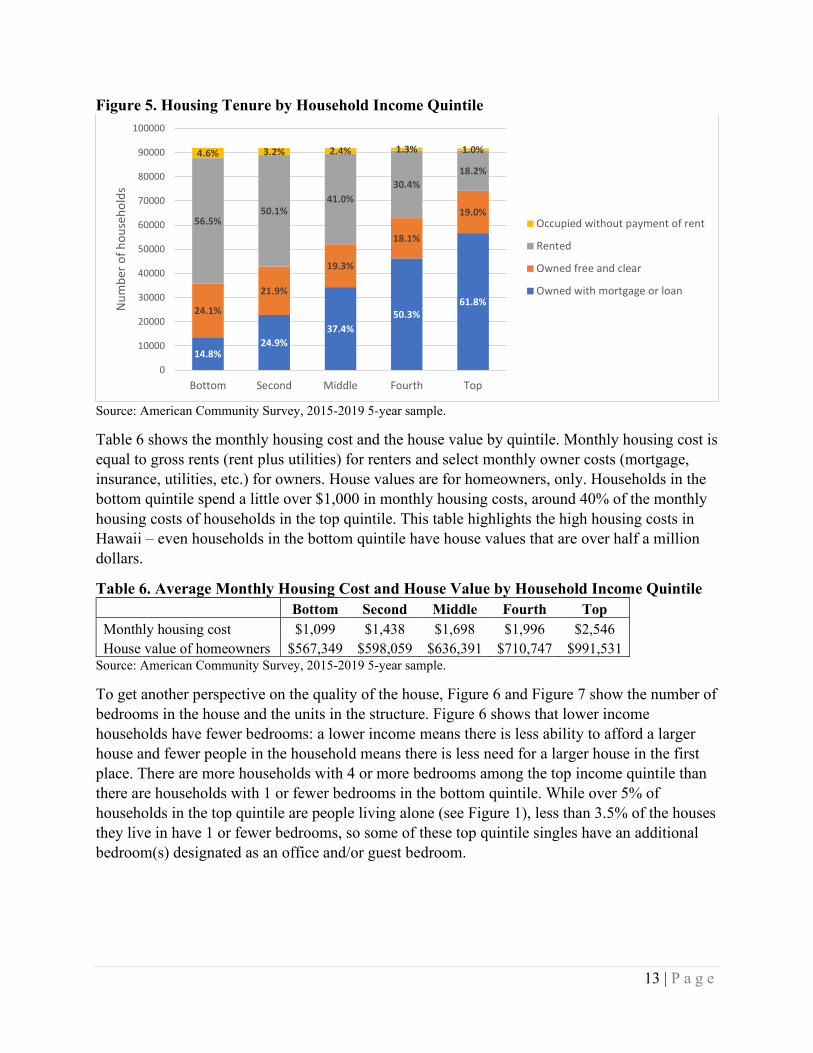
How does household income translate into the type of housing one resides in? Unsurprisingly, lower income households cannot accumulate as many savings as higher income households, and are far more likely to be in a rental unit (Figure 5); over half of households in the bottom and second quintiles rent their living space, compared to less than 20% for the top income quintile. However, the lowest income quintiles are more likely to own their house free and clear compared to the higher income quintiles, by 3-5 percentage points. There are two possibilities for why this could be the case. First, as noted in Figure 3 above, lower income households tend to be headed by older householders, increasing the likelihood that the mortgage has been paid off. Second, because of having low income, people could be living in their childhood home that has already been paid off.

65.7% 67.8% 68.6% 68.5% 66.2%

27.6% 24.9% 24.8% 25.3% 27.6%

0

10000

20000

30000

40000

50000

60000

70000

80000

90000

100000

Bottom Second Middle Fourth Top

Num

ber o

f hou

seho

lds

Other languages

Asian and Pacific Island languages

Other Indo-European languages

Spanish

English only

13 | P a g e

Figure 5. Housing Tenure by Household Income Quintile

Source: American Community Survey, 2015-2019 5-year sample.

Table 6 shows the monthly housing cost and the house value by quintile. Monthly housing cost is equal to gross rents (rent plus utilities) for renters and select monthly owner costs (mortgage, insurance, utilities, etc.) for owners. House values are for homeowners, only. Households in the bottom quintile spend a little over $1,000 in monthly housing costs, around 40% of the monthly housing costs of households in the top quintile. This table highlights the high housing costs in Hawaii – even households in the bottom quintile have house values that are over half a million dollars.

Table 6. Average Monthly Housing Cost and House Value by Household Income Quintile Bottom Second Middle Fourth Top Monthly housing cost $1,099 $1,438 $1,698 $1,996 $2,546 House value of homeowners $567,349 $598,059 $636,391 $710,747 $991,531

Source: American Community Survey, 2015-2019 5-year sample.

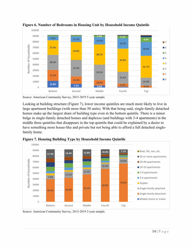
To get another perspective on the quality of the house, Figure 6 and Figure 7 show the number of bedrooms in the house and the units in the structure. Figure 6 shows that lower income households have fewer bedrooms: a lower income means there is less ability to afford a larger house and fewer people in the household means there is less need for a larger house in the first place. There are more households with 4 or more bedrooms among the top income quintile than there are households with 1 or fewer bedrooms in the bottom quintile. While over 5% of households in the top quintile are people living alone (see Figure 1), less than 3.5% of the houses they live in have 1 or fewer bedrooms, so some of these top quintile singles have an additional bedroom(s) designated as an office and/or guest bedroom.

14.8%24.9%

37.4%50.3%

61.8%24.1%

21.9%

19.3%

18.1%

19.0%56.5%

50.1%41.0%

30.4%18.2%

4.6% 3.2% 2.4% 1.3% 1.0%

0

10000

20000

30000

40000

50000

60000

70000

80000

90000

100000

Bottom Second Middle Fourth Top

Num

ber o

f hou

seho

lds

Occupied without payment of rent

Rented

Owned free and clear

Owned with mortgage or loan

14 | P a g e

Figure 6. Number of Bedrooms in Housing Unit by Household Income Quintile

Source: American Community Survey, 2015-2019 5-year sample.

Looking at building structure (Figure 7), lower income quintiles are much more likely to live in large apartment buildings (with more than 50 units). With that being said, single-family detached homes make up the largest share of building type even in the bottom quintile. There is a minor bulge in single-family detached homes and duplexes (and buildings with 3-4 apartments) in the middle three quintiles that disappears in the top quintile that could be explained by a desire to have something more house-like and private but not being able to afford a full detached single-family home.

Figure 7. Housing Building Type by Household Income Quintile

Source: American Community Survey, 2015-2019 5-year sample.

12.8% 7.2% 4.4%

21.2%

14.4%10.0%

6.1% 3.3%

28.3%

31.2%

29.5%

22.4%

15.0%

27.6%33.8%

38.2%

44.0%

41.7%

7.6% 11.1% 14.3%19.3%

26.6%

2.9% 5.1%8.9%

0

10000

20000

30000

40000

50000

60000

70000

80000

90000

100000

Bottom Second Middle Fourth Top

Num

ber o

f hou

seho

lds

7

6

5

4

3

2

1

0

43.3% 46.0% 52.1%62.8%

73.0%

7.4%11.5%

11.1%

10.2%

10.0%

17.3% 14.4% 12.8% 10.0% 7.1%

0

10000

20000

30000

40000

50000

60000

70000

80000

90000

100000

Bottom Second Middle Fourth Top

Num

ber o

f hou

seho

lds

Boat, RV, van, etc.

50 or more apartments

20-49 apartments

10-19 apartments

5-9 apartments

3-4 apartments

Duplex

Single family attached

Single family detached

Mobile home or trailer

15 | P a g e

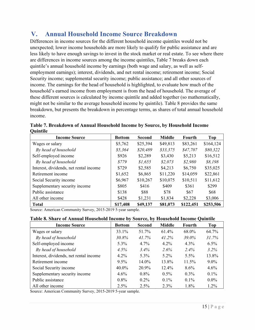
V. Annual Household Income Source Breakdown Differences in income sources for the different household income quintiles would not be unexpected; lower income households are more likely to qualify for public assistance and are less likely to have enough savings to invest in the stock market or real estate. To see where there are differences in income sources among the income quintiles, Table 7 breaks down each quintile’s annual household income by earnings (both wage and salary, as well as self-employment earnings); interest, dividends, and net rental income; retirement income; Social Security income; supplemental security income; public assistance; and all other sources of income. The earnings for the head of household is highlighted, to evaluate how much of the household’s earned income from employment is from the head of household. The average of these different sources is calculated by income quintile and added together (so mathematically, might not be similar to the average household income by quintile). Table 8 provides the same breakdown, but presents the breakdown in percentage terms, as shares of total annual household income.

Table 7. Breakdown of Annual Household Income by Source, by Household Income Quintile

Income Source Bottom Second Middle Fourth Top Wages or salary $5,762 $25,394 $49,813 $83,261 $164,124 By head of household $5,364 $20,489 $33,375 $47,707 $80,322 Self-employed income $926 $2,289 $3,430 $5,213 $16,512 By head of household $779 $1,655 $2,073 $2,980 $8,198 Interest, dividends, net rental income $729 $2,585 $4,213 $6,750 $35,025 Retirement income $1,652 $6,865 $11,220 $14,059 $22,861 Social Security income $6,967 $10,267 $10,075 $10,511 $11,612 Supplementary security income $805 $416 $409 $361 $299 Public assistance $138 $88 $78 $67 $68 All other income $428 $1,231 $1,834 $2,228 $3,006 Total $17,408 $49,137 $81,073 $122,451 $253,506

Source: American Community Survey, 2015-2019 5-year sample.

Table 8. Share of Annual Household Income by Source, by Household Income Quintile Income Source Bottom Second Middle Fourth Top

Wages or salary 33.1% 51.7% 61.4% 68.0% 64.7% By head of household 30.8% 41.7% 41.2% 39.0% 31.7% Self-employed income 5.3% 4.7% 4.2% 4.3% 6.5% By head of household 4.5% 3.4% 2.6% 2.4% 3.2% Interest, dividends, net rental income 4.2% 5.3% 5.2% 5.5% 13.8% Retirement income 9.5% 14.0% 13.8% 11.5% 9.0% Social Security income 40.0% 20.9% 12.4% 8.6% 4.6% Supplementary security income 4.6% 0.8% 0.5% 0.3% 0.1% Public assistance 0.8% 0.2% 0.1% 0.1% 0.0% All other income 2.5% 2.5% 2.3% 1.8% 1.2%

Source: American Community Survey, 2015-2019 5-year sample.

16 | P a g e

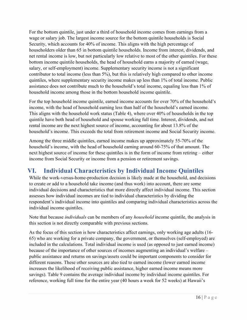
For the bottom quintile, just under a third of household income comes from earnings from a wage or salary job. The largest income source for the bottom quintile households is Social Security, which accounts for 40% of income. This aligns with the high percentage of householders older than 65 in bottom quintile households. Income from interest, dividends, and net rental income is low, but not particularly low relative to most of the other quintiles. For these bottom income quintile households, the head of household earns a majority of earned (wage, salary, or self-employment) income. Supplementary security income is not a significant contributor to total income (less than 5%), but this is relatively high compared to other income quintiles, where supplementary security income makes up less than 1% of total income. Public assistance does not contribute much to the household’s total income, equaling less than 1% of household income among those in the bottom household income quintile.

For the top household income quintile, earned income accounts for over 70% of the household’s income, with the head of household earning less than half of the household’s earned income. This aligns with the household work status (Table 4), where over 40% of households in the top quintile have both head of household and spouse working full time. Interest, dividends, and net rental income are the next highest source of income, accounting for about 13.8% of the household’s income. This exceeds the total from retirement income and Social Security income.

Among the three middle quintiles, earned income makes up approximately 55-70% of the household’s income, with the head of household earning around 60-75% of that amount. The next highest source of income for these quintiles is in the form of income from retiring – either income from Social Security or income from a pension or retirement savings.

VI. Individual Characteristics by Individual Income Quintiles While the work-versus-home-production decision is likely made at the household, and decisions to create or add to a household take income (and thus work) into account, there are some individual decisions and characteristics that more directly affect individual income. This section assesses how individual incomes are tied to individual characteristics by dividing the respondent’s individual income into quintiles and comparing individual characteristics across the individual income quintiles.

Note that because individuals can be members of any household income quintile, the analysis in this section is not directly comparable with previous sections.

As the focus of this section is how characteristics affect earnings, only working age adults (16-65) who are working for a private company, the government, or themselves (self-employed) are included in the calculations. Total individual income is used (as opposed to just earned income) because of the importance of other sources of incomes augmenting an individual’s welfare – public assistance and returns on savings/assets could be important components to consider for different reasons. These other sources are also tied to earned income (lower earned income increases the likelihood of receiving public assistance, higher earned income means more savings). Table 9 contains the average individual income by individual income quintiles. For reference, working full time for the entire year (40 hours a week for 52 weeks) at Hawaii’s

17 | P a g e

minimum wage ($10.10 an hour) means an annual income of $21,008. The self-sufficiency wage for one adult in Hawaii is just over $35,000 in 201812.

Table 9. Average Annual Individual Income by Individual Income Quintile Bottom Second Middle Fourth Top Individual income $9,168 $26,433 $41,052 $61,515 $132,511

Source: American Community Survey, 2015-2019 5-year sample.

Table 10 shows how the worker is related to the head of household by individual income quintile. Over 30% of the workers in the bottom quintile are children of the head of household, so there might be less concern for the average individual income for this quintile ($9,168) being less than a third of the single adult self-sufficiency wage. However, over 35% of people in this quintile are either the head of household or spouse/partner, and so a couple with each partner earning in the bottom quintile would fall significantly below the self-sufficiency wage. Further, some of these children could be adult children still living with their parents. Almost 60% of the top quintile workers are heads of household, and over a quarter of workers in this quintile are the spouse/partner.

Table 10. Relationship to Household Head by Individual Income Quintile % of Workers in Quintile

Relationship to Household Head Bottom Second Middle Fourth Top Head of household 22.2% 29.3% 38.3% 47.2% 59.4% Opposite-sex husband/wife/spouse 13.5% 16.8% 20.5% 24.3% 24.9% Opposite-sex unmarried partner 2.6% 3.4% 2.9% 2.9% 1.6% Same-sex husband/wife/spouse 0.1% 0.2% 0.2% 0.3% 0.3% Same-sex unmarried partner 0.1% 0.3% 0.3% 0.3% 0.2% Biological son or daughter 30.0% 19.3% 16.5% 10.1% 5.7% Adopted son or daughter 0.8% 0.5% 0.4% 0.2% 0.1% Stepson or stepdaughter 1.3% 0.7% 0.5% 0.3% 0.2% Brother or sister 2.8% 3.6% 2.9% 2.0% 1.0% Father or mother 1.0% 1.4% 0.6% 0.6% 0.4% Grandchild 4.4% 1.9% 1.4% 0.8% 0.3% Parent-in-law 0.3% 0.4% 0.1% 0.1% 0.1% Son-in-law or daughter-in-law 2.4% 3.0% 3.0% 2.2% 1.4% Other relative 4.6% 4.6% 3.2% 2.1% 0.9% Roommate or housemate 3.4% 3.6% 3.3% 3.1% 1.4% Other nonrelative 4.6% 4.4% 4.8% 3.0% 1.8% Group quarters population 5.7% 6.9% 1.2% 0.4% 0.1%

Source: American Community Survey, 2015-2019 5-year sample. Note: Foster children omitted from calculations due to small sample size. Columns might not sum to100% due to rounding.

12 Department of Business, Economic Development and Tourism. (2019). Self-Sufficiency Income Standard: Estimates for Hawaii 2018. Available at https://files.hawaii.gov/dbedt/economic/reports/self-sufficiency/self-sufficiency_2018.pdf.

18 | P a g e

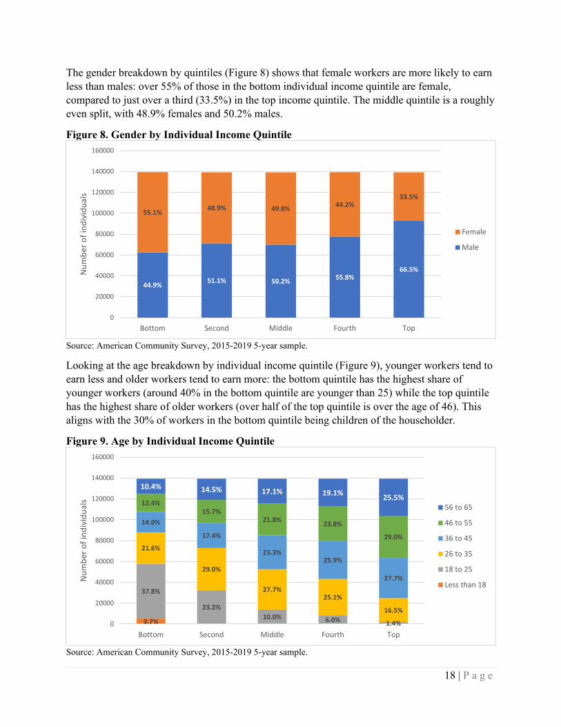
The gender breakdown by quintiles (Figure 8) shows that female workers are more likely to earn less than males: over 55% of those in the bottom individual income quintile are female, compared to just over a third (33.5%) in the top income quintile. The middle quintile is a roughly even split, with 48.9% females and 50.2% males.

Figure 8. Gender by Individual Income Quintile

Source: American Community Survey, 2015-2019 5-year sample.

Looking at the age breakdown by individual income quintile (Figure 9), younger workers tend to earn less and older workers tend to earn more: the bottom quintile has the highest share of younger workers (around 40% in the bottom quintile are younger than 25) while the top quintile has the highest share of older workers (over half of the top quintile is over the age of 46). This aligns with the 30% of workers in the bottom quintile being children of the householder.

Figure 9. Age by Individual Income Quintile

Source: American Community Survey, 2015-2019 5-year sample.

44.9% 51.1% 50.2% 55.8%66.5%

55.1% 48.9% 49.8% 44.2%33.5%

0

20000

40000

60000

80000

100000

120000

140000

160000

Bottom Second Middle Fourth Top

Num

ber o

f ind

ivid

uals

Female

Male

3.7%

37.8%

23.2%10.0% 6.0% 1.4%

21.6%

29.0%

27.7%25.1%

16.5%

14.0%

17.4%

23.3%25.9%

27.7%

12.4%15.7%

21.8% 23.8%

29.0%

10.4% 14.5% 17.1% 19.1% 25.5%

0

20000

40000

60000

80000

100000

120000

140000

160000

Bottom Second Middle Fourth Top

Num

ber o

f ind

ivid

uals 56 to 65

46 to 55

36 to 45

26 to 35

18 to 25

Less than 18

19 | P a g e

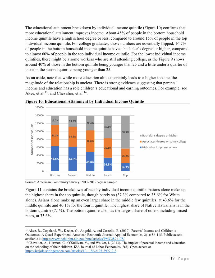
The educational attainment breakdown by individual income quintile (Figure 10) confirms that more educational attainment improves income. About 45% of people in the bottom household income quintile have a high school degree or less, compared to around 15% of people in the top individual income quintile. For college graduates, those numbers are essentially flipped; 16.7% of people in the bottom household income quintile have a bachelor’s degree or higher, compared to almost 60% of people in the top individual income quintile. For the lower individual income quintiles, there might be a some workers who are still attending college, as the Figure 9 shows around 40% of those in the bottom quintile being younger than 25 and a little under a quarter of those in the second quintile being younger than 25.

As an aside, note that while more education almost certainly leads to a higher income, the magnitude of the relationship is unclear. There is strong evidence suggesting that parents’ income and education has a role children’s educational and earning outcomes. For example, see Akee, et al.13, and Chevalier, et al.14.

Figure 10. Educational Attainment by Individual Income Quintile

Source: American Community Survey, 2015-2019 5-year sample.

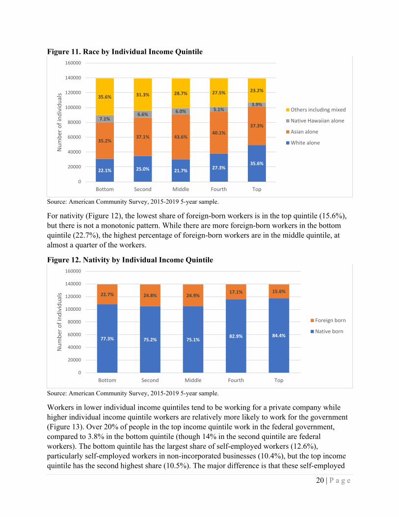
Figure 11 contains the breakdown of race by individual income quintile. Asians alone make up the highest share in the top quintile, though barely so (37.3% compared to 35.6% for White alone). Asians alone make up an even larger share in the middle few quintiles, at 43.6% for the middle quintile and 40.1% for the fourth quintile. The highest share of Native Hawaiians is in the bottom quintile (7.1%). The bottom quintile also has the largest share of others including mixed races, at 35.6%.

13 Akee, R., Copeland, W., Keeler, G., Angold, A, and Costello, E. (2010). Parents’ Income and Children’s Outcomes: A Quasi-Experiment. American Economic Journal: Applied Economics, 2(1): 86-115. Public access available at https://www.ncbi.nlm.nih.gov/pmc/articles/PMC2891175/. 14 Chevalier, A., Harmon, C., O’Sullivan, V., and Walker, I. (2013). The impact of parental income and education on the schooling of their children. IZA Journal of Labor Economics, 2(8). Open access at https://izajole.springeropen.com/articles/10.1186/2193-8997-2-8.

45.6% 44.6%34.8%

24.8%14.9%

37.7% 36.2%

38.8%

35.1%

26.2%

16.7% 19.3%26.4%

40.1%

58.9%

0

20000

40000

60000

80000

100000

120000

140000

160000

Bottom Second Middle Fourth Top

Num

ber o

f ind

ivid

uals

Bachelor's degree or higher

Associates degree or some college

High school diploma or less

20 | P a g e

Figure 11. Race by Individual Income Quintile

Source: American Community Survey, 2015-2019 5-year sample.

For nativity (Figure 12), the lowest share of foreign-born workers is in the top quintile (15.6%), but there is not a monotonic pattern. While there are more foreign-born workers in the bottom quintile (22.7%), the highest percentage of foreign-born workers are in the middle quintile, at almost a quarter of the workers.

Figure 12. Nativity by Individual Income Quintile

Source: American Community Survey, 2015-2019 5-year sample.

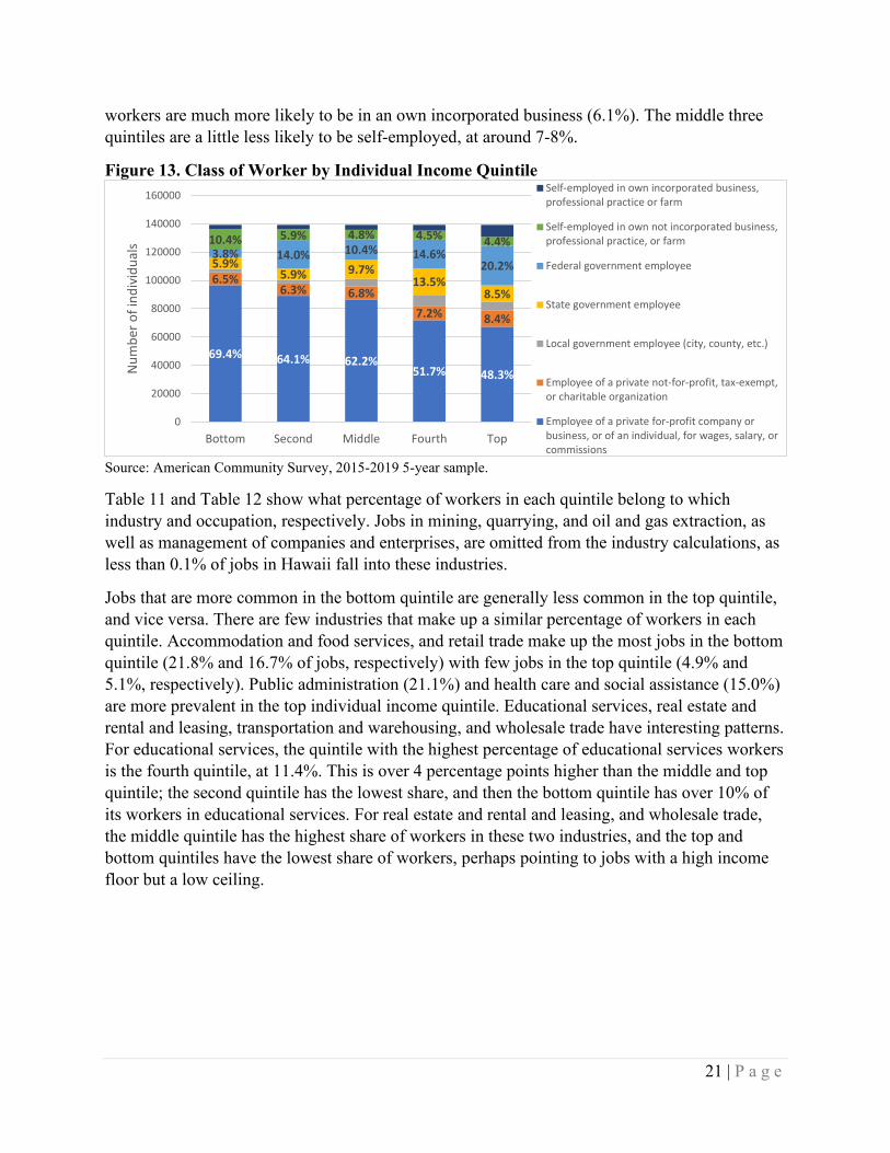
Workers in lower individual income quintiles tend to be working for a private company while higher individual income quintile workers are relatively more likely to work for the government (Figure 13). Over 20% of people in the top income quintile work in the federal government, compared to 3.8% in the bottom quintile (though 14% in the second quintile are federal workers). The bottom quintile has the largest share of self-employed workers (12.6%), particularly self-employed workers in non-incorporated businesses (10.4%), but the top income quintile has the second highest share (10.5%). The major difference is that these self-employed

22.1% 25.0% 21.7% 27.3%35.6%

35.2%37.1% 43.6%

40.1%37.3%

7.1%6.6% 6.0% 5.1%

3.9%35.6% 31.3% 28.7% 27.5% 23.2%

0

20000

40000

60000

80000

100000

120000

140000

160000

Bottom Second Middle Fourth Top

Num

ber o

f ind

ivid

uals

Others including mixed

Native Hawaiian alone

Asian alone

White alone

77.3% 75.2% 75.1%82.9% 84.4%

22.7% 24.8% 24.9%17.1% 15.6%

0

20000

40000

60000

80000

100000

120000

140000

160000

Bottom Second Middle Fourth Top

Num

ber o

f ind

ivid

uals

Foreign born

Native born

21 | P a g e

workers are much more likely to be in an own incorporated business (6.1%). The middle three quintiles are a little less likely to be self-employed, at around 7-8%.

Figure 13. Class of Worker by Individual Income Quintile

Source: American Community Survey, 2015-2019 5-year sample.

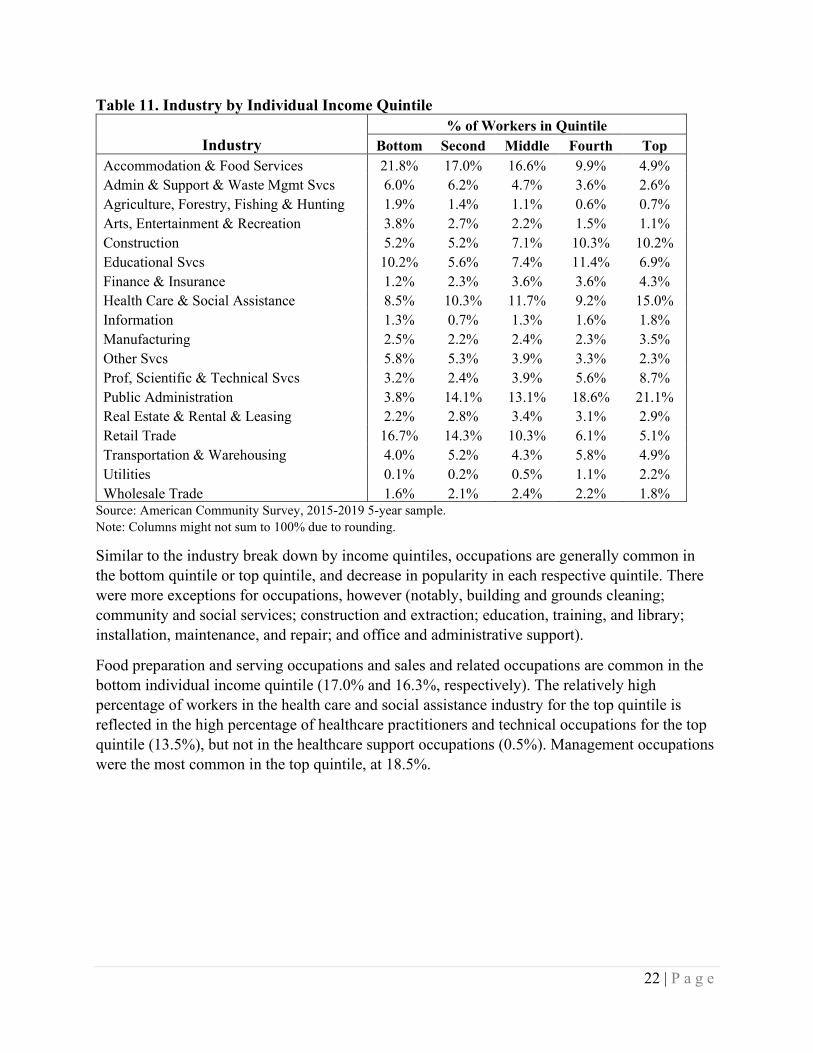
Table 11 and Table 12 show what percentage of workers in each quintile belong to which industry and occupation, respectively. Jobs in mining, quarrying, and oil and gas extraction, as well as management of companies and enterprises, are omitted from the industry calculations, as less than 0.1% of jobs in Hawaii fall into these industries.

Jobs that are more common in the bottom quintile are generally less common in the top quintile, and vice versa. There are few industries that make up a similar percentage of workers in each quintile. Accommodation and food services, and retail trade make up the most jobs in the bottom quintile (21.8% and 16.7% of jobs, respectively) with few jobs in the top quintile (4.9% and 5.1%, respectively). Public administration (21.1%) and health care and social assistance (15.0%) are more prevalent in the top individual income quintile. Educational services, real estate and rental and leasing, transportation and warehousing, and wholesale trade have interesting patterns. For educational services, the quintile with the highest percentage of educational services workers is the fourth quintile, at 11.4%. This is over 4 percentage points higher than the middle and top quintile; the second quintile has the lowest share, and then the bottom quintile has over 10% of its workers in educational services. For real estate and rental and leasing, and wholesale trade, the middle quintile has the highest share of workers in these two industries, and the top and bottom quintiles have the lowest share of workers, perhaps pointing to jobs with a high income floor but a low ceiling.

69.4% 64.1% 62.2%51.7% 48.3%

6.5%6.3% 6.8%

7.2% 8.4%

5.9%5.9% 9.7%

13.5%8.5%

3.8% 14.0% 10.4% 14.6%20.2%

10.4% 5.9% 4.8% 4.5% 4.4%

0

20000

40000

60000

80000

100000

120000

140000

160000

Bottom Second Middle Fourth Top

Num

ber o

f ind

ivid

uals

Self-employed in own incorporated business,professional practice or farm

Self-employed in own not incorporated business,professional practice, or farm

Federal government employee

State government employee

Local government employee (city, county, etc.)

Employee of a private not-for-profit, tax-exempt,or charitable organization

Employee of a private for-profit company orbusiness, or of an individual, for wages, salary, orcommissions

22 | P a g e

Table 11. Industry by Individual Income Quintile % of Workers in Quintile

Industry Bottom Second Middle Fourth Top Accommodation & Food Services 21.8% 17.0% 16.6% 9.9% 4.9% Admin & Support & Waste Mgmt Svcs 6.0% 6.2% 4.7% 3.6% 2.6% Agriculture, Forestry, Fishing & Hunting 1.9% 1.4% 1.1% 0.6% 0.7% Arts, Entertainment & Recreation 3.8% 2.7% 2.2% 1.5% 1.1% Construction 5.2% 5.2% 7.1% 10.3% 10.2% Educational Svcs 10.2% 5.6% 7.4% 11.4% 6.9% Finance & Insurance 1.2% 2.3% 3.6% 3.6% 4.3% Health Care & Social Assistance 8.5% 10.3% 11.7% 9.2% 15.0% Information 1.3% 0.7% 1.3% 1.6% 1.8% Manufacturing 2.5% 2.2% 2.4% 2.3% 3.5% Other Svcs 5.8% 5.3% 3.9% 3.3% 2.3% Prof, Scientific & Technical Svcs 3.2% 2.4% 3.9% 5.6% 8.7% Public Administration 3.8% 14.1% 13.1% 18.6% 21.1% Real Estate & Rental & Leasing 2.2% 2.8% 3.4% 3.1% 2.9% Retail Trade 16.7% 14.3% 10.3% 6.1% 5.1% Transportation & Warehousing 4.0% 5.2% 4.3% 5.8% 4.9% Utilities 0.1% 0.2% 0.5% 1.1% 2.2% Wholesale Trade 1.6% 2.1% 2.4% 2.2% 1.8%

Source: American Community Survey, 2015-2019 5-year sample. Note: Columns might not sum to 100% due to rounding.

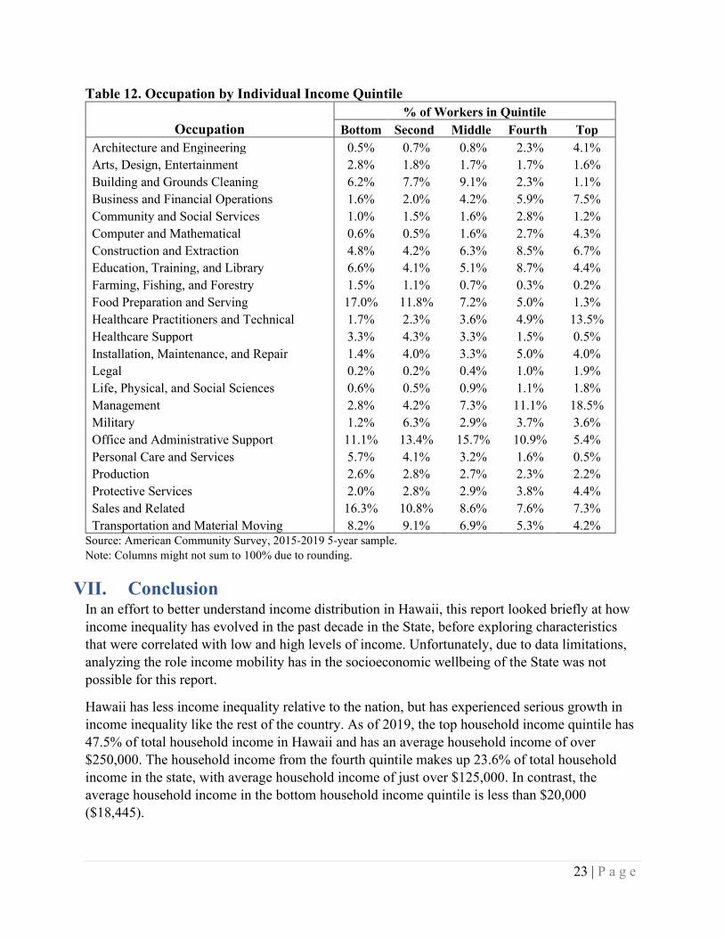
Similar to the industry break down by income quintiles, occupations are generally common in the bottom quintile or top quintile, and decrease in popularity in each respective quintile. There were more exceptions for occupations, however (notably, building and grounds cleaning; community and social services; construction and extraction; education, training, and library; installation, maintenance, and repair; and office and administrative support).

Food preparation and serving occupations and sales and related occupations are common in the bottom individual income quintile (17.0% and 16.3%, respectively). The relatively high percentage of workers in the health care and social assistance industry for the top quintile is reflected in the high percentage of healthcare practitioners and technical occupations for the top quintile (13.5%), but not in the healthcare support occupations (0.5%). Management occupations were the most common in the top quintile, at 18.5%.

23 | P a g e

Table 12. Occupation by Individual Income Quintile % of Workers in Quintile

Occupation Bottom Second Middle Fourth Top Architecture and Engineering 0.5% 0.7% 0.8% 2.3% 4.1% Arts, Design, Entertainment 2.8% 1.8% 1.7% 1.7% 1.6% Building and Grounds Cleaning 6.2% 7.7% 9.1% 2.3% 1.1% Business and Financial Operations 1.6% 2.0% 4.2% 5.9% 7.5% Community and Social Services 1.0% 1.5% 1.6% 2.8% 1.2% Computer and Mathematical 0.6% 0.5% 1.6% 2.7% 4.3% Construction and Extraction 4.8% 4.2% 6.3% 8.5% 6.7% Education, Training, and Library 6.6% 4.1% 5.1% 8.7% 4.4% Farming, Fishing, and Forestry 1.5% 1.1% 0.7% 0.3% 0.2% Food Preparation and Serving 17.0% 11.8% 7.2% 5.0% 1.3% Healthcare Practitioners and Technical 1.7% 2.3% 3.6% 4.9% 13.5% Healthcare Support 3.3% 4.3% 3.3% 1.5% 0.5% Installation, Maintenance, and Repair 1.4% 4.0% 3.3% 5.0% 4.0% Legal 0.2% 0.2% 0.4% 1.0% 1.9% Life, Physical, and Social Sciences 0.6% 0.5% 0.9% 1.1% 1.8% Management 2.8% 4.2% 7.3% 11.1% 18.5% Military 1.2% 6.3% 2.9% 3.7% 3.6% Office and Administrative Support 11.1% 13.4% 15.7% 10.9% 5.4% Personal Care and Services 5.7% 4.1% 3.2% 1.6% 0.5% Production 2.6% 2.8% 2.7% 2.3% 2.2% Protective Services 2.0% 2.8% 2.9% 3.8% 4.4% Sales and Related 16.3% 10.8% 8.6% 7.6% 7.3% Transportation and Material Moving 8.2% 9.1% 6.9% 5.3% 4.2%

Source: American Community Survey, 2015-2019 5-year sample. Note: Columns might not sum to 100% due to rounding.

VII. Conclusion In an effort to better understand income distribution in Hawaii, this report looked briefly at how income inequality has evolved in the past decade in the State, before exploring characteristics that were correlated with low and high levels of income. Unfortunately, due to data limitations, analyzing the role income mobility has in the socioeconomic wellbeing of the State was not possible for this report.

Hawaii has less income inequality relative to the nation, but has experienced serious growth in income inequality like the rest of the country. As of 2019, the top household income quintile has 47.5% of total household income in Hawaii and has an average household income of over $250,000. The household income from the fourth quintile makes up 23.6% of total household income in the state, with average household income of just over $125,000. In contrast, the average household income in the bottom household income quintile is less than $20,000 ($18,445).

24 | P a g e

Household size is positively correlated with income, with an average household size of 1.86 for the bottom quintile, growing to 3.85 for the top quintile. This could both be a cause and effect relationship; smaller households have fewer people to earn income, while having less income discourages adding non-earning members to the household. These smaller households in the bottom income quintile mean over half of these households are single householders with no spouse/partner, children, or non-relative present. Over three quarters of top quintile households are married couple households, with about two thirds of these married couple households not having any own children under 18 present in the household. Comparing work experience, almost a quarter of households in the bottom household income quintile have neither the householder or spouse working, whereas in the top quintile, 40% of these households have both spouses working full time. The head of household for top income quintiles are more likely to be male and in prime earning age (36-55 years old); the head of household for lower income quintiles are more likely to be female and older than 65 (retired and not earning much income) or younger than 25 (not enough work experience to be earning high income).

While top household income quintile households are far more likely to own their house compared to the lower income quintiles (over 68% in the top quintile compared to just under 29% for the bottom quintile), the lower income quintiles are more likely to own their house free and clear, 24% compared to 18%. Smaller household sizes among the bottom quintile means houses tend to be smaller from a number-of-bedrooms perspective. Lower income quintile households are less likely to be in a single family detached home and more likely to be in a large apartment complex. Among homeowners, the bottom income quintile has an average house value of under $570,000, compared to the top quintile average house value of around $990,000.

Breaking down income sources by income quintile, bottom income quintile households have a lower share of their income coming from wage and salary (33.1%) and investments/equity (4.2%) compared to the top income quintile households (64.7% and 13.8%, respectively). In contrast, Social Security, supplementary security, and public assistance income makes up 45.4% of the lowest quintile’s household income, compared to 4.7% for the top income quintile households.

To more directly look at how individual characteristics affect individual income, this report compared individual characteristics of working-age (16-65 years old) adults who are working for a private company, the government, or themselves (self-employed) by individual income quintile. The average individual income for the top quintile was almost 15 times that of the bottom quintile (approximately $132,500 versus approximately $9,200). Workers in the top individual income quintile tended to be male, older, and with a bachelor’s degree or higher. They were more likely to work for the federal government and less likely to work at a for-profit business. Top quintile workers tended to work in the government, health care, or construction industries, whereas bottom quintile workers were more concentrated in the tourism-related industries (accommodations and food services, retail). With regards to occupation, top quintile workers tended to be in health care or management occupations, while bottom quintile workers were more likely to work in food preparation, office support, or sales.