Analyzing Runoff Dynamics of Paved Soil Surface

Using Weighable Lysimeters

vorgelegt vonDipl.-Ing.

Yong-Nam Rimaus Pyongyang, Korea (DVR)

Von der Fakultat VI - Planen | Bauen | Umweltder Technischen Universitat Berlin

zur Erlangung des akademischen GradesDoktor der Ingenieurwissenschaften

- Dr. -Ing. -

genehmigte Dissertation

Promotionsausschuss:

Vorsitzender: Prof. Dr. Bernd-Michael WilkeBerichter: Prof. Dr. Gerd WessolekBerichter: Prof. Dr. Wilfred Endlicher

Tag der wissenschaftlichen Aussprache: 28.04.2011

Berlin 2011

D83

2

Danksagung

Mein großter Dank gilt Prof. Dr. Gerd Wessolek, dass er mir als “Außenste-hender” die Moglichkeit gab, an seinem Fachgebiet wissenschaftlich arbeiten zukonnen. Danke fur das Verstandnis, die herzliche Forderung und das mir stetsentgegengebrachte Vertrauen. Dank ihm weiß ich, was wissenschaftliches Ar-beiten heißt und wie man es anfangt.

Weiterer Dank gilt Prof. Dr. Wilfred Endlicher fur die Bereitschaft, meine Ar-beit zu begutachten, vor allem dafur, dass er mir als Sprecher des gesamtenGraduiertenkollegs wertvolle Impulse gab und mich motivierte, forderte und mireine außergewohnliche Sichtweise des Forschens vermittelte.

Ich danke Dr. Thomas Nehls ganz herzlichst dafur, dass er mit Geduld, Verstandnisund breiter Diskussion meine Forschungsarbeit angeleitet, mit offenen Ohrenmeiner wenigen Kenntnis großes Selbsbewusstsein geschenkt und mich die ganzeStrecke lang herzlich begleitet hat.

Ohne die wissenschaftstechnische und praktische Wegleitung durch Dr. SteffenTrinks ware das Projekt so nicht zustande gekommen. Ich danke ihm fur dietatkraftige Unterstutzung, besonders wahrend der Anfangsphase meiner Arbeit.

Weiterhin danke an Dr. Norbert Litz fur die Verfugbarkeit der Lysimeterstationund Dr. Norbert Markwardt fur die Kooperation beim technischen Aufbau derAnlage. Mein Dank gilt auch an Herrn Michael Facklam, Karl Botscher und FrauUte Lesner fur die Hilfe an den regnerischen und windigen Tagen wahrend desAufbaus und der Fertigstellung der Lysimeteranlage sowie an Dr. Bjorn Kluge,Alexandra Toland und Dr. Andre Peters fur die vielen Diskussionen und Anre-gungen.

Allen Doktoranden des DFG-Graduiertenkollegs “Stadtokologische Perspektiven780/3” gilt mein Dank fur die gemeinsame, freudige Zeit der Ausbildung zu “Stad-texperten”.

Schließlich danke ich meinen Eltern und Schwester fur das Vertrauen, das langeWarten, Geduld und all das, was ich heute bin, ganz besonders fur die stetigeZuversicht uber meine Entscheidung.

3

Preface

I studied the urban water balance, especially the runoff dynamics of permeablepavements. My work was initiated within the Graduate School “Perspectiveson Urban Ecology” (DFG-GRK 780/3). This interdisciplinary research programhas been supported by German Science Foundation (Deutsche Forschungsgemein-schaft) and represented by Prof. Dr. Wilfred Endlicher at the Department Gerog-raphy of Humboldt Universitat zu Berlin. DFG-GRK 780/3 has included projectsin social and natural sciences and started in 2002 at Humboldt Universitat zuBerlin, Technische Universitat Berlin, and Freie Universitat Berlin. Since then,the three phases concentrated on different topics:

Cohort 1 (2002–2005): Perspectives on Urban Ecology I - The Example ofthe European Metropolis of Berlin

Cohort 2 (2005–2008): Perspectives on Urban Ecology II - Shrinking cities:structural changes as opportunities for the development of urban nature andenhanced environmental quality for city dwellers

Cohort 3 (2008–2011): Perspectives on Urban Ecology III - Optimizing urbannature development–Dynamic change of nature functions and the urban environ-ment of city dwellers.

The aim of my (third) cohort (2008–2011) was to understand the functionsof ecological processes in the city impacting the quality of life for urban humanpopulation. Scenarios take into account the profound issues of change in climate,demographics, economy, and all their consequences for nature and environmentin metropolitan areas. The chosen interdisciplinary approach integrated the fol-lowing research clusters:

Cluster 1 - Optimize ecological functions and biodiversity of urban roadsides

Cluster 2 - Reuse of former housing estates and urban brownfields

Cluster 3 - Strategies for temporarily used urban sites

Cluster 4 - Psychological health and mental state of urban dwellers

My work, as a part of cluster 1, was developed from the two predecessorprojects in the graduate school. Dr. Thomas Nehls investigated the proper-ties of paved urban soils and the sorption and transport of heavy metals (Nehls,2007). Dr. Eva Klingelmann studied leaching of the pesticide glyphosate from

4

urban pavements (Klingelmann, 2009). Both studies suffered from the lack ofprocess-based hydrologic model for paved soils in their solute transport simula-tions. Therefore, I started with the aim to develop such a process-based modelfrom lysimeter experiments. I hope that the expanded understanding of urbanrunoff processes contributes to the improvement of life circumstances for urbandwellers.

December 2010.

5

Summary

Soil hydrology investigates the dynamic equilibrium between precipitation, runoff,evapotranspiration, and infiltration processes at the soil surface. Although it isknown that these dynamic processes also play a role for fully and partly paved soilsurfaces, the departments of urban water managements have mostly understoodsurface hydrologic processes in terms of simplified and empiric model. The runoffcoefficient for the design storms allows the quantification of the occurring surfacerunoff water. Such a rational approach was the basic concept for flood-orientedurban design.

In consideration of urban adaption strategies to climate change and watershortages, it becomes clear that process-based models are necessary in order topredict the availability of water resources with high temporal and spatial reso-lution. Surface water is no more to get lost, but to be available for utilization.This clearly reflects the paradigm change to the resource-oriented handling withthe rainwater in urban areas.

Many studies investigated the effective parameters for describing runoff be-haviors only based on the runoff measurement from the paved surfaces. However,in order to develop a process-based model, the observation and the measurementof all water balance components in their relationship are necessary.

The aim of the study is to develop a process-based model for runoff dynamics.For the representative elementary area of paved soil surfaces, the water balanceprocesses were measured under varying natural hydrologic conditions, using theweighable paved lysimeter system. In order to observe the runoff dynamics evenfrom small events, a new runoff setup, called the weighable tipping bucket (WTB),was developed.

Based on the measurement from the weighable lysimeter system, a model forintensity-dependent surface storage and runoff was developed. The surface hy-drologic parameters for two typical pavement types, Bernburg mosaic cobblestoneand Concrete paving slab, were determined. The fundamental knowledge is to beestablished in order to understand and describe the functions of pavement as onecompensation factor for urban water budget. The upper boundary conditionsof the lysimeter attempted to simulate the real urban soil surfaces. The urbanwater budget processes were continuously observed for the climate and hydro-logic conditions of Berlin, Germany for the period between May 2009 and April

6

2010. The components, such as precipitation, evaporation, runoff and ground-water recharge were measured with the resolution of 0.1 mm/min. The annualrunoff coefficients were ca. 16 % and 27 %, respectively, for Bernburg mosaic cob-blestone and Concrete paving slab. These results were considerably smaller thanthe results predicted from the standard regulations (e.g. DWA-Regeln). Thesurface storage and the rainfall event intensity were derived as the main factorfrom the analysis of runoff-producing rainfall events.

The process-based model of runoff dynamics describes the runoff coefficientin relationship with the rainfall event intensity, r, the surface storage, Vs, therunoff-producing intensity, ro, the final infiltration rate, b, and the infiltrationexponent, n.

RC = f (r) =

1− Vs

P ·

(1−

ro

r· tanh

r

ro

) ·

(1− R−R 1

n

(1− n) · (1−R 1n )

)

The surface storage determines the total potential of pavement for the infiltra-tion capacity through the rainfall event. The smaller the rainfall event intensity,the more effective the buffer function of the surface storage becomes. Hence,the runoff behavior of small and middle-strong precipitation events clearly dif-fers from that of storm events. While the runoff coefficient for the small eventsrapidly increases together with the increasing intensity, the runoff coefficients re-mains relatively constant for the storm events with great intensity, depending ofthe paving materials.

Throughout the adaption of these models to the observed precipitation events,the average effective values for the surface hydrologic parameters are determinedfor the two pavements. The surface storages amounted to ca. 0.9 mm and 0.4 mm,the runoff-producing intensities to ca. 0.02 mm/min and 0.01 mm/min, the finalinfiltration rates to 0.016 mm/min and 0.012 mm/min, and the infiltration ex-ponents to ca. 2.5 and 0.7, respectively, for Bernburg mosaic cobblestone andConcrete paving slab.

In this study, a process-based model concept for describing the dynamic runoffbehaviors of paved soil surfaces was developed for the first time and applied totwo different pavement types. The improvement of the lysimeter technique byusing a weighable tipping bucket enabled the high-resolution measurement ofrunoff processes. A technical and analytical method could be established toderive the surface hydrologic parameters for further paving materials. This isimportant for the quantification and improvement of retention capacity for newmaterials in the sense of pavement renewing potential. For example, during the

7

measurement period, the utilization of the mosaic cobblestones has shown 1.7-fold smaller runoff in comparison with the concrete paving slabs. The modelclarified that the surface storage has to be adjusted to the characteristics ofregional precipitation frequency in order to minimize the runoff water.

The process-based model allows assessing the uncertainty of the predictionfrom the simplified empiric models. It can be applied to the various climateconditions.

8

Zusammenfassung

Die Bodenhydrologie untersucht die dynamischen Gleichgewichte zwischen Niede-rschlag sowie Abfluss-, Verdunstungs- und Infiltrationsprozessen an Bodenoberfla-chen. Zwar spielen diese dynamischen Prozesse auch fur die versiegelten und teil-versiegelten Flachen eine Rolle, allerdings fasst die Siedlungswasserwirtschaft dieentsprechenden Prozesse bislang in vereinfachten empirischen Modellen zusam-men. Der Abflussbeiwert fur maximale Bemessungsregen ermoglicht die Quan-tifizierung des anfallenden Wassers. Das Model bildet so die konzeptionelleGrundlage fur die entwasserungskomfort- und hochwasserschutzorientierte Stadt-planung.

Im Zuge der Diskussion um die urbane Anpassungsstrategie an den Kli-mawandel und die Wasserknappheit wird deutlich, dass prozessbasierte Mod-elle benotigt werden. Damit kann die Verfugbarkeit vom Niederschlagsabfluss-wasser auch unter sich andernden klimatischen Bedingungen raumlich und zeitlichhochaufgelost berechnet werden. Wahrend also Wasser in der Vergangenheit “an-fiel”, wird es in Zukunft “verfugbar” sein. Dies spiegelt deutlich den Paradigmen-wechsel hinzu einem ressourcen-orientierten Umgang mit dem Regenwasser in derStadt wider.

Zahlreiche Studien ermittelten effektive Parameter zur Beschreibung des Abflu-sses nur aus Abflussmessungen auf versiegelten Flachen. Fur die Entwicklungeines prozessbasierten Modells wird jedoch die Erfassung aller Wasserhaushalt-skomponenten im Zusammenhang notig.

Das Ziel der Arbeit ist, ein prozessbasiertes Modell fur die Beschreibung desdynamischen Abflussverhaltens zu entwickeln. Die Arbeit untersucht dafur denWasserhaushalt teilversiegelter reprasentativer Elementarflachen unter naturlichvariierenden Niederschlagsbedingungen mittels hochauflosender wagbarer Lysime-ter. Um die Dynamik der Abflussprozesse auch fur kleine Niederschlagsereignisseuntersuchen zu konnen, wurde ein neues Messinstrument, die wagbare Kipp-waage, entwickelt.

Daraus wurde ein Modell fur die intensitatsabhangige Oberflachenspeicherungund Abfluss abgeleitet. Die oberflachen-hydrologischen Parameter fur die amhaufigsten benutzten urbanen Flachenmaterialien wurden bestimmt. Damit solldie Grundlage geschafft werden, die Funktion der teilversiegelten Flachen als Aus-gleichsraum fur das Stadtklima herauszuarbeiten. Unter der realitatsnahen Ver-

9

wirklichung der oberen Randbedingung der Lysimeter wurde das durchgangigeurbane Wasserhaushaltsgeschehen fur das Klima- und Niederschlagsverhaltnisvom Berlin gemessen. Im Untersuchungsjahr zwischen Mai 2009 und April 2010wurden die Wasserhaushaltskomponenten, Niederschlag, Verdunstung, Abflussund Grundwasserneubildung, sowohl fur Bernburger Mosaikpflaster als auch furGroßbetonsteinplatte mit einer Auflosung von minimal 0.1 mm/min aufgezeich-net. Dabei wurde ein Oberflachenabfluss von insgesamt ca. 16 % des Nieder-schlags fur das Bernburg Mosaik und ca. 27 % fur die Großbetonsteinplatte er-mittelt. Diese Werte sind deutlich geringer als die Werte, die mittels Abflussbei-werten aus Regelwerken prognostiziert wurden. Durch Analyse der abflusswirk-samen Ereignisse wurden der Oberflachenspeicher und die Intensitat der Nieder-schlagsereignisse als bestimmende Faktoren abgeleitet.

Das prozess-basierte Modell des dynamischen Oberflachenabflusses beschreibtden Abflussbeiwert in Abhangigkeit von der Niederschlagsintensitat, r, dem Ober-flachenspeicher, Vs, der abflusswirksamen Intensitat, ro, der Endinfiltrationsrate,b und dem Infiltrationsexponent, n.

RC = f (r) =

1− Vs

P ·

(1−

ro

r· tanh

r

ro

) ·

(1− R−R 1

n

(1− n) · (1−R 1n )

)

Der Oberflachenspeicher bestimmt die Abflusswirksamkeit und den gesamtenProzess des Abflusses. Die Pufferfunktion des Oberflachenspeichers ist umsoeffektiver, je kleiner die Niederschlagsintensitat und je großer die Endinfiltra-tionsrate ist. Daher unterscheidet sich das Abflussverhalten wahrend schwacherbis mittelstarker Ereignisse deutlich vom Abflussverhalten bei Starkregenereignis-sen. Wahrend der Abflussbeiwert fur die schwachen bis mittelstarken Nieder-schlagsereignisse mit steigender Intensitat rasch steigt, bleibt er fur großere In-tensitaten materialabhangig relativ konstant.

Durch die Anpassung dieses Modells an die beobachteten Ereignisse wur-den die mittleren wirksamen oberflachen-hydrologischen Parameter fur die zweiPflasterarten bestimmt. Der Oberflachenspeicher betragt ca. 0,9 mm bzw. ca.0,4 mm, die abflusswirksame Intensitat ca. 0,02 mm/min, bzw. ca. 0,01 mm/min,die Endinfiltrationsrate 0,016 mm/min bzw. 0,012 mm/min und der Infiltration-sexponent ca. 2,5 bzw. ca. 0,7 jeweils fur das Bernburg Mosaik bzw. dieBetonsteinplattepflaster.

In dieser Arbeit wurde erstmals ein prozessbasiertes Modell fur die Beschrei-bung des Oberflachenabflussverhaltens teilversiegelter Flachen entwickelt und aufzwei verschiedene Teilversiegelungsarten angewendet. Durch die Erweiterung

10

der Lysimetertechnik um die wagbare Kippwaage zur hochauflosenden Erfassungdes Oberflachenabflusses wurde eine technische und analytische Methodik furdie Ableitung der Flachenparameter auch anderer Versiegelungsmaterialien en-twickelt. Damit konnen die Retentionskapazitaten neuer Materialien im Sinnedes Belagsanderungspotenzials gemessen und verbessert werden. Zum Beispielfuhrte die Gestaltung teilversiegelter Flachen mit Bernburger Mosaik im Vergle-ich zu Betonsteinplatten im Beobachtungszeitraum zu einem 1,7-fach verringertenAbfluss. Das Modell verdeutlicht, dass der Oberflachenspeicher auf die Nieder-schlagsverteilung abgestimmt werden muss, um den Oberflachenabfluss zu min-imieren.

Das prozessbasierte Modell ermoglicht die Abschatzung der Unsicherheitender Prognosen vereinfachter empirischer Modelle. Das Modell kann weiterhin aufunterschiedliche Klimabedingungen angewendet werden.

11

Contents

Preface 3

Summary 6

I Introduction 19

1 Background and Motivation 201.1 Background of Pavement Hydrology . . . . . . . . . . . . . . . . . 201.2 Aims and Hypothesis . . . . . . . . . . . . . . . . . . . . . . . . . 24

2 Urban Soil Water Budget - State of the Art 272.1 Lysimeter Studies on Urban Water Balance . . . . . . . . . . . . 272.2 Models for Runoff and Infiltration Processes . . . . . . . . . . . . 34

II Materials and Method 40

3 Developing the Paved Weighable Lysimeter System 413.1 General Aspects of Lysimeters . . . . . . . . . . . . . . . . . . . . 423.2 Measurement of the Water Budget Components . . . . . . . . . . 44

3.2.1 Lysimeter Setup . . . . . . . . . . . . . . . . . . . . . . . . 443.2.2 Pavement Assembly with “Berlin’s Sidewalk” . . . . . . . 503.2.3 General Runoff Assembly . . . . . . . . . . . . . . . . . . 53

3.3 Data Acquisition and Handling . . . . . . . . . . . . . . . . . . . 55

4 A New Technical Approach for Measuringthe Runoff Dynamics 594.1 General Aspects of Runoff Measurements . . . . . . . . . . . . . . 594.2 Weighable Tipping Bucket . . . . . . . . . . . . . . . . . . . . . . 634.3 Increased Accuracy of Surface Runoff

Measurement using WTB . . . . . . . . . . . . . . . . . . . . . . 65

12

III Results and Discussion 72

5 Water Balance of Paved Soil 735.1 Precipitation Event Separation . . . . . . . . . . . . . . . . . . . 73

5.1.1 Precipitation Event Parameterson Small Field Plots of Lysimeter . . . . . . . . . . . . . . 74

5.1.2 Determination of Event Separation Criteria . . . . . . . . 765.1.3 Cumulative Precipitation Frequency Functions . . . . . . . 78

5.2 Annual Precipitation-Event Frequency . . . . . . . . . . . . . . . 805.3 Water Balance 2009–2010 . . . . . . . . . . . . . . . . . . . . . . 82

5.3.1 Groundwater Recharge and Evaporation . . . . . . . . . . 825.3.2 Influence of Rainfall-Runoff Relationship

on Water Balance . . . . . . . . . . . . . . . . . . . . . . . 86

6 Model Concept for Runoff Dynamicsof Paved Soil Surface 926.1 Surface Water Process . . . . . . . . . . . . . . . . . . . . . . . . 93

6.1.1 Phase of Runoff and Infiltration Process . . . . . . . . . . 936.1.2 Runoff Coefficient . . . . . . . . . . . . . . . . . . . . . . . 96

6.2 Surface Storage Model . . . . . . . . . . . . . . . . . . . . . . . . 996.2.1 Runoff Concentration Process . . . . . . . . . . . . . . . . 996.2.2 Surface Storage Model using Hyperbolic Tangent . . . . . 103

6.3 Runoff Coefficient Model . . . . . . . . . . . . . . . . . . . . . . . 1066.3.1 Description of Rain-pond Infiltration Process . . . . . . . . 1066.3.2 Intensity-dependent Runoff Coefficient

for Small Field Plot under Constant Rainfall Flux . . . . . 108

7 Determination of Surface Hydrological Parameters 1127.1 Results from Surface Storage Model . . . . . . . . . . . . . . . . . 1127.2 Results from Intensity-dependent RC Model . . . . . . . . . . . . 115

Conclusions and Outlook 119

Bibliography 121

13

List of Figures

1.1 Typical road cross sections from ancient Roman times and fromBerlin of 19th century. . . . . . . . . . . . . . . . . . . . . . . . . 21

1.2 Urban water balance for Berlin compared to its suburbs (Nehlset al., 2006). . . . . . . . . . . . . . . . . . . . . . . . . . . . . . . 23

2.1 An example of standard vertical structure of sidewalk: Lysimetersurface scheme used by Flotter (2006). . . . . . . . . . . . . . . . 32

2.2 Decomposition of rainfall event by SCS rainfall-runoff relationship(McCuen, 2004). . . . . . . . . . . . . . . . . . . . . . . . . . . . 36

3.1 Lysimeter location in Marienfelde, southern Berlin, Germany. . . . 443.2 Lysimeter site in the experiment field of UBA (Federal Agency for

Environment). . . . . . . . . . . . . . . . . . . . . . . . . . . . . . 453.3 Scheme of paved weighable lysimeter. . . . . . . . . . . . . . . . . 463.4 Lysimeter basement. . . . . . . . . . . . . . . . . . . . . . . . . . 473.5 Sand-bedding as pavement base. . . . . . . . . . . . . . . . . . . . 473.6 Gathering seepage water at the lower boundary. . . . . . . . . . . 483.7 Capillary blocking layer from gravel. . . . . . . . . . . . . . . . . 483.8 Water column and runoff discharge pipe: the water column pro-

vides suction plates with a sub-pressure of ca. 63 hP. The runoffdischarge pipe carries the runoff down from the runoff gutter. . . 49

3.9 Lysimeter surface with the materials of “Berlin’s Walkway”. . . . 513.10 Water pouring to consolidate the seam material and runoff water

flowing to runoff gutter. . . . . . . . . . . . . . . . . . . . . . . . 543.11 Lysimeter surface section. . . . . . . . . . . . . . . . . . . . . . . 543.12 Lysimeter data stream. . . . . . . . . . . . . . . . . . . . . . . . . 553.13 Hellmann gauge in 30 cm level from the paved surface in lysimeter

station. . . . . . . . . . . . . . . . . . . . . . . . . . . . . . . . . . 573.14 Precipitation event measured by Hellmann gauge and paved weigh-

able lysimeter. . . . . . . . . . . . . . . . . . . . . . . . . . . . . . 58

4.1 Contributution of small events to the whole water balance. . . . . 614.2 Weighable tipping bucket for accurate runoff measurement. . . . . 63

14

4.3 Improved mass resolution: Runoff event from concrete pavementat the 3rd of September 2009. . . . . . . . . . . . . . . . . . . . . 70

4.4 Improved temporal resolution: Runoff event from concrete pave-ments on September 3rd, 2009. . . . . . . . . . . . . . . . . . . . . 71

5.1 Parameters of the runoff-effective precipitation event process. . . . 755.2 Determination of the separation criterion for precipitation events. 775.3 An example of precipitation events from Oct. 8th 2009 . . . . . . 795.4 The cumulative precipitation depth PF (r) and the cumulative

event number NF (r). . . . . . . . . . . . . . . . . . . . . . . . . . 815.5 Annual water balance 2009/10. . . . . . . . . . . . . . . . . . . . 835.6 Paved surfaces induced a big deficit of evaporation in comparison

with the grass reference surface (FAO lysimeter). . . . . . . . . . 855.7 Runoff-producing and non-producing precipitation-events. . . . . 905.8 Runoff coefficients versus rainfall event intensity. . . . . . . . . . . 91

6.1 Three phases of runoff process from a precipitation event from Juli23rd, 2009. . . . . . . . . . . . . . . . . . . . . . . . . . . . . . . . 95

6.2 Precipitation-runoff relationship of pavement from Burnburg mo-saic cobblestone and Concrete paving slab. . . . . . . . . . . . . . 98

6.3 Initial loss (Pa) versus precipitation depth (P ). . . . . . . . . . . . 1006.4 Surface storage. . . . . . . . . . . . . . . . . . . . . . . . . . . . . 1026.5 The tangent hyperbolic function. . . . . . . . . . . . . . . . . . . 1046.6 Surface storage model for the runoff concentration process. . . . . 1056.7 Rain-pond infiltration (i(t) = infiltration [mm/min], t = time [min]).1076.8 The theoretical relationship between the runoff coefficient (RCu)

and the rainfall event intensity (r). . . . . . . . . . . . . . . . . . 1106.9 The theoretical relationship between the runoff coefficient (RCu)

and the the relative infiltrability (R). . . . . . . . . . . . . . . . . 111

7.1 Adaption of the surface storage model and determination of thesurface storage, Vs, and the runoff-producing intensity, ro. . . . . . 114

7.2 Adaption of the intensity-dependent runoff coefficient model anddetermination of the final infiltration , b, and the infiltration ex-ponent, n. . . . . . . . . . . . . . . . . . . . . . . . . . . . . . . . 116

15

List of Tables

2.1 Surface hydrologic parameters for pavements of cobblestone andpaving slab from Leipzig by Schramm (1996) . . . . . . . . . . . . 28

2.2 Water balance for pavements of Bernburg mosaic cobblestone andConcrete paving slab from Berlin by Wessolek (1993, 1994) . . . . 29

2.3 Surface hydrologic parameters for pavements of Bernburg mosaiccobblestone and Concrete paving slab from Berlin by Wessolek(1993, 1994); Wessolek and Facklam (1997). . . . . . . . . . . . . 30

2.4 Water balance for pavements of concrete cobblestone and pavingslab from Hamburg by Flotter (2006). . . . . . . . . . . . . . . . . 32

2.5 Surface hydrologic parameters for pavements of concrete cobble-stone and paving slab by Flotter (2006). . . . . . . . . . . . . . . 33

3.1 Parameter of lysimeter pavements. Almost identical seam materialand sub-base structure are used for both pavements of Bernburgcobblestone and Concrete paving slabs. . . . . . . . . . . . . . . . 52

5.1 Monthly water balance components and runoff coefficients. . . . . 865.2 Monthly precipitation-event frequency. . . . . . . . . . . . . . . . 875.3 The distribution of runoff-producing and non-runoff-producing rain-

fall events in the period of 2009/10. . . . . . . . . . . . . . . . . . 885.4 The average runoff coefficients of event ranges according to the

intensity. . . . . . . . . . . . . . . . . . . . . . . . . . . . . . . . . 89

7.1 Surface hydrologic parameters for pavements of Bernburg mosaiccobblestone and Concrete paving slab. . . . . . . . . . . . . . . . 117

16

List of Abbreviations

Abbreviation Meaning

a infiltration capacity parameter

A size of catchment area [ha]

b final infiltration rate for saturated soil [mm/min]

CPS concrete paving slab

d seam portion

∆W changeable water storage in soil [mm]

Es evapotranspiration of sealed area [mm]

Eu evapotranspiration of unsealed area [mm]

ET evapotranspiration [mm]

F actual retention capacity [mm] or [l/ha]

GW groundwater recharge [mm]

I infiltration depth [mm] or [l/ha]

i(t) infiltration function [mm/min]

ir average infiltration capacity [mm/min]

MCS Bernburg mosaic cobblestone

n infiltration exponent

n number of rainfall event

n event number

NF (r) cumulative event frequency function

P set of rainfall events

P precipitation depth [mm] or [l/ha]

Pa initial loss [mm]

Pe effective precipitation [mm]

Pn nth event as set element, characterized by intensity rn,

depth Pn, duration tn, or rainfall pattern

17

Pu effective rainfall depth while soil is unsaturated [mm]

PF (r) cumulative precipitation frequency function

P[r] set of rainfall events of intensity r

P (r) total precipitation sum of P[r]

Ps effective rainfall depth after soil is saturated [mm]

p(t) precipitation intensity [mm/min]

Q actual runoff sum [mm] or [l/ha]

q(t) runoff intensity [mm/min]

r rainfall event intensity

ro runoff-producing intensity [mm/min]

RC runoff coefficient

RCe effective runoff coefficient

RCu runoff coefficient during unsaturated infiltration process (tc < t < ts)

RCe runoff coefficient during saturated infiltration process (t ≥ ts)RO runoff sum [mm] or [l/ha]

T precipitation duration [min]

tc time point of runoff beginning

Tc runoff concentration duration [min]

TB tipping bucket

Td precipitation separation criterion (time span

between rainfall events) [min]

Te effective precipitation duration (tp − tc) [min]

tp time point of precipitation ending

ts time point of saturation

Vs surface water storage or surface storage [mm]

Vp porous volume of paving material [mm]

Vsm porous volume of seam material [mm]

Vr infiltrated water of initial loss [mm]

WTB weighable tipping bucket

18

Part I

Introduction

19

Chapter 1

Background and Motivation

1.1 Background of Pavement Hydrology

Functions of Pavements

Pavements have been used to seal streets and roads for 4000 years. They fulfillimportant functions as technical infrastructure in cities. Pavements allow citydwellers to emancipate from the natural circumstances such as muddy soils inrainy weather. Paved ways are drained, in order to provide a profound, dry, andreliable way for fast transport of goods and people. Usually, during construction,also a leveling of the way is gained. These were the main purposes to buildroads in ancient times e.g. the “Via Militaris” in the Roman Empire, as well as“Autobahnen” nowadays (see Fig. 1.1).

Paved streets and ways canalized movements and transport, they connectedand divided the parts of the city. Therefore, pavements structured the city, anddue to numerous design possibilities, they forged the architectural identity forthe cities.

From the hygienic viewpoints, pavements in connection with sewage systemscontributed to clean housing and helped to minimize epidemics like cholera. Afterall, soil sealing enables convenient city life and urban prosperity, nevertheless, italso provides ecological habitat functions for plant and animals.

Effects of Soil Sealing

In Berlin, the degree of soil sealing is nearly 34 % of the urban landscape. 11 %are covered by buildings, 13 % are sealed without buildings, and 10 % are streets.Depending on the quarter, soil sealing varies between 20 % and 66 %, however,around two thirds of this is always made up of public streets and walkways whichare considered as “partly sealed areas” (Senatsverwaltung Berlin fur Stadten-twicklung, 2001).

20

(a) Ancient Roman street.

(b) Berlin street from 19th century.

Figure 1.1: Typical road cross sections (a) from Roman times (Fusch,2010: on-line. http://cc.owu.edu) and (b) from Berlin 19th century (Schladweiler et al. 2010: on-line. http://sewerhistory.org). Note that the sewage system is an important feature of soilsealing.

21

Soil sealing is highly anthropogenic in many respects: the spatial distributionand vertical construction of paved surface, the material properties that composethe pavement and the hydrological aftereffects on the urban watershed. Soil seal-ing induces alterations of nature in urban areas, leading to a number of ecologicaland economic problems for city dwellers and the surrounding population. Thus,urban environment obtains completely a different circumstance in result (Nehlset al., 2006).

Despite such a high degree of soil sealing, it has not yet gained a significantimportance for the sense of common social perception. Therefore the Federal Lawfor Soil Protection has not yet defined soil sealing as soil impairment. Soil sealingis mentioned in the law only as one of several possibilities for blocking harmed soilmaterial, in order to prevent its mobilization by wind and water erosion or inflowof harmful substances from the atmosphere into the groundwater zone (Wessolek,2001). However, the impact of soil sealing has been recognized for long time inrespects of extreme urban water balance, urban heat stress, and quality of urbanwater resources.

Firstly, soil sealing has a crucial effect on the urban water balance due tointerruption of the water exchange process between pedosphere and atmosphere.It is known that the average runoff can increase enormously through soil sealing,while infiltration is confined to remain as optimal as in natural soils (Fig. 1.2).For paved soil surfaces, the reduction of evaporation is a significant problem forurban micro-climates in the summer period. The reason is presumably the smallstorage capacity of paved surfaces (Flotter, 2006; Gobel et al., 2007; Starke, 2010).The evaporation can be exponentially increased by increasing the soil openingratio (also called “seam portion”). Therefore, purposeful selection of pavementsand suitable implementation can positively affect the urban water balance andclimate, e.g. through the use of porous pavements with big seam portions andhigh surface storage (Nakayama and Fujita, 2010).

Secondly, it is evidenced that the surface water resource of urban area isreducing due to the modified urban water budget. This leads to distinctive tem-perature fluctuation with heightened average. The affected urban heat balanceresults clearly in high heat stress (Endlicher, 2008). Compared to the unsealedsurrounding areas, the average annual temperature increases by 0.5 to 1 K withabsolute maximum differences of up to 10 K (Kuttler, 1998). This so called “urbanheat island effect” leads to human health problems and to increased macroeco-nomic costs in these areas (Tol, 2002; Townsend et al., 2003). The urban heatisland effect cannot be completely avoided by desealing measures, but its impacton the human population can be decreased by using water-sharing pavements.

Thirdly, problems of surface water dynamics lead to further troubles for urbanwater quality (Heinzmann, 1998; Akan and Houghtalen, 2003). Because the urbansoils are persistently exposed to emissions and immissions, the seam materials–the soil between the paving stones on pavements–which acts as flow path forinfiltration and capillary rising, is strongly modified over the years with urban

22

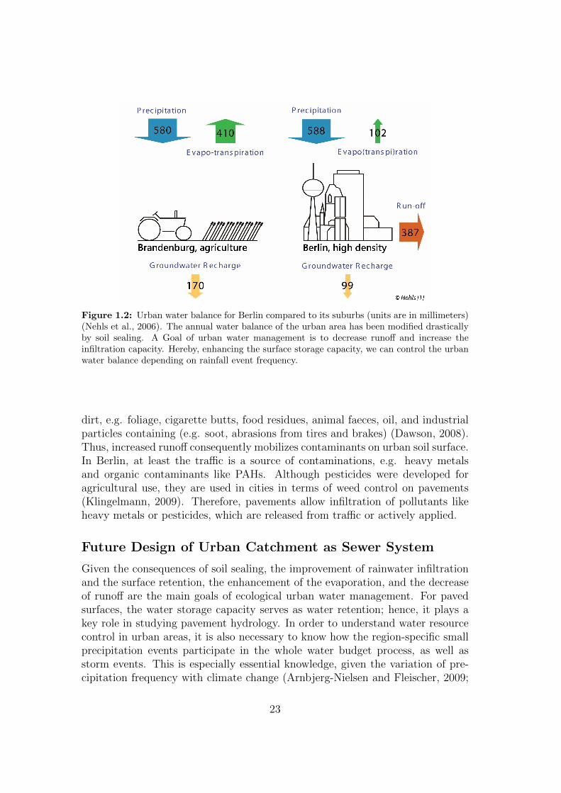
Figure 1.2: Urban water balance for Berlin compared to its suburbs (units are in millimeters)(Nehls et al., 2006). The annual water balance of the urban area has been modified drasticallyby soil sealing. A Goal of urban water management is to decrease runoff and increase theinfiltration capacity. Hereby, enhancing the surface storage capacity, we can control the urbanwater balance depending on rainfall event frequency.

dirt, e.g. foliage, cigarette butts, food residues, animal faeces, oil, and industrialparticles containing (e.g. soot, abrasions from tires and brakes) (Dawson, 2008).Thus, increased runoff consequently mobilizes contaminants on urban soil surface.In Berlin, at least the traffic is a source of contaminations, e.g. heavy metalsand organic contaminants like PAHs. Although pesticides were developed foragricultural use, they are used in cities in terms of weed control on pavements(Klingelmann, 2009). Therefore, pavements allow infiltration of pollutants likeheavy metals or pesticides, which are released from traffic or actively applied.

Future Design of Urban Catchment as Sewer System

Given the consequences of soil sealing, the improvement of rainwater infiltrationand the surface retention, the enhancement of the evaporation, and the decreaseof runoff are the main goals of ecological urban water management. For pavedsurfaces, the water storage capacity serves as water retention; hence, it plays akey role in studying pavement hydrology. In order to understand water resourcecontrol in urban areas, it is also necessary to know how the region-specific smallprecipitation events participate in the whole water budget process, as well asstorm events. This is especially essential knowledge, given the variation of pre-cipitation frequency with climate change (Arnbjerg-Nielsen and Fleischer, 2009;

23

Faram et al., 2010). Water budget components may be considered as dynamicprocesses. This can help us select suitable paving types, e.g. cobblestones andconcrete paving slabs with sufficient openings, in order to reach the goals men-tioned above.

A typical urban landscape mostly consists of street canyon, building facadesand roof surfaces, and urban greens. There are modern urban strategies suchas the innovative adiabatic cooling technology for indoor space and the greeningtechnology for building facades and roofs, not to mention about the efforts toretain natural urban greens (Dreiseitl and Grau, 2009).

Because, from economic and social reasons, those innovative ambitioned tech-nologies are not always and everywhere possible in the city areas–especially forthe big cities such as Berlin, more technical adaption and fundamental knowledgeare necessary to control the urban water resources.

Design of sewer systems needs to challenge with the existing uncertainty ofbasic data and to differentiate its safety concept. The pavements are considereda crucial part of urban sewer system, especially in the background of the futuredemographic development and the predicted climate change. The illustrationof the detailed runoff transportation in urban areas and its interplay with theprecipitation will become more and more a routine-task for model calibration andplausibility. Therefore, a process-based modeling of urban catchment graduallybecomes indispensable task of pavement hydrology (Pecher and Hoppe, 2011).

1.2 Aims and Hypothesis

A goal of conventional urban water management was the fast drainage of surfaceflow to protect the urban catchment area from floods. Another goal was tocontrol water pollution for urban water systems by separating runoff completelyfrom the original water cycle. These led to the development of hydrologicalapproach aimed at removing surface water as fast and far as possible towardsoutlet channels and wastewater treatment plants. Urban sewer systems weredesigned and continuously improved for the cases of storm events. This approachallowed cities to develop rapidly till the middle of last century (Geiger et al.,2009).

However, after the 1950s, the significant disadvantage of this approach wasrecognized in the point of economical and ecological view for residential waterengineering and management systems. After the “Separated Rainwater Man-agement” had been established and practiced for several decades, many regionsand communities are nowadays working to decentralize municipal rainwater man-agement so that sustainable urban development is ensured by a more holisticapproach to urban water resources (Pecher and Hoppe, 2011).

Many numerical models and operational tools were developed for describingthe urban water catchment area more precisely in order to reconnect the urban

24

surface flow with natural water cycle. These attempts still could not go beyondthe principles of its regional redistribution and reallocation. The design storms–arainfall event of specified size and return frequency (i.e., a storm what has thelikelihood of occurring once every 10 or 100 years) that is used to calculate therunoff volume and peak discharge rate–are still the key input factor for dimen-sioning the rainwater management system (ATV-DVWK, 1992; IPS, 2005; Kwon,2008; Sieker et al., 2009; Bronstert et al., 2006).

From an urban hydrologic viewpoint, permeable pavement is preferable tototal sealing because it provides improved water retention capacity. Here, thesurface water storage is a key parameter. It is presumably used up differently forthe rainfall events, depending on the pavement types. For instance, small rainfallevents result in much different surface water behavior than the design stormevents. This behavior finally influences on the annual water balance (Ferguson,2005).

Several studies have indicated that permeable pavements impacts dynamicallyon water balance processes according to soil hydrologic and climatic conditions(Flotter, 2006; Glugla and Krahe, 1995; Schramm, 1996). The dynamic runoffbehaviors were described by using operational algorithms, but not able to bemathematically interpreted. The infiltration process was a complex interactionof many sub-processes that are too complicated to mathematically describe.

The previous models developed for urban water balance embed the classicalapproaches which do not parameterize the reaction of disturbed urban surfacessuch as the rational runoff approach and SCS approach. The concept family ofHorton’s infiltration was the first attempt at modeling dynamic water infiltration,but it had been originally used for modeling large natural watershed areas (seeChap. 2.1).

There is still the question how far the paved soils can show the potentialfor the improved urban water balance and which surface parameter is the mostimportant for explaining the runoff dynamics. Surface storage capacity is likelyto include parameters such as seam portion, porosity of pavement and initial soilconductivity. But its clear influence on runoff and infiltration has not yet beenderived (Borgwardt, 2006).

The main hypothesis of the work is that the paved soil surface can play apositive role for the improvement of the urban water balance, when they areadjusted to the regional precipitation characteristics. Furthermore, this dynam-ically depends on the interplay between the soil surface and the rainfall eventparameters.

The final aim of the study is to develop a process-based model for runoffdynamics of paved soil surfaces. A paved weighable lysimeter system will be de-signed and constructed, especially for runoff measurement from the representativeelementary area of two typical pavements of Berlin: Bernburg mosaic cobblestoneand Concrete paving slab. The annual water balance process will be analyzedprofoundly in the relationship with the precipitation frequency. After the runoff

25

and the infiltration processes are physically described, the surface storage andthe runoff coefficient will be clarified as function of rainfall intensity and surfacehydrologic parameters. By applying these model concepts to the measured datafrom experiment period between 2009 and 2010, the surface hydrologic parame-ters for the two typical pavement types will be determined. In sum, it is aimed togain the basic knowledge needed to improve urban water resource managementby better controlling urban surface water resources.

26

Chapter 2

Urban Soil Water Budget - Stateof the Art

Over the last 20 years, a number of studies on urban water budget have beencarried out. Experimentally, these studies have been based on either lysimeteror lab studies according to research object and extent. Lysimeter studies (alsoknown as “Lysimetery”) have enabled researchers to look at the physical andhydrological phenomena in soils as a whole, incorporating the true complexityof paved soils, while lab studies have focused on certain individual processes.Since priority of these studies was given to flood protection and the related eco-nomic interests, the studies, primarily runoff studies, have focused on the cases ofstorm events. Results from these studies provided the technical specifications andstandards with maximum runoff coefficient and minimum conductivity of mostpaving materials. From this state of knowledge, urban planning and water engi-neering have resulted in economic and ecological risks. The potential of partlypaved surfaces are underestimated and the sewer infrastructures are overdimen-sioned (DIN 1986-3, 1986; ATV-DVWK, 1992; Sieker et al., 2003; DWA-A, 2005;Borgwardt et al., 2000; ATV-DVWK, 2000; DWA-A, 2006).

In this chapter, some selected lysimeter studies are reviewed. Their results areanalyzed in comparison to the hydrologic potential of paved surfaces for urbanwater budgets. Overviews of some runoff and infiltration models will provide afundamental conceptual model of surface water processes.

2.1 Lysimeter Studies on Urban Water Balance

Glugla and Krahe (1995) studied urban runoff generation from the hydrologic-economic and resource-emphasized aspects. They considered the role of regionaltypical small events for surface retention and evaporation. For regions of Berlin,they clarified that the surface storage capacity of sealed areas presumably playeda decisive role for the total continuous water supply of the inner-city system of

27

Table 2.1: Surface hydrologic parameters for pavements of cobblestone and paving slab fromLeipzig by Schramm (1996). ir = final infiltration rate, RCmax = max. runoff coefficient, Vs =surface storage, and d = seam portion.

RC max i r V s d[%] [mm/min] [mm] [%]

r = 0.6 mm/min, T = 60 min 82.0 0.10

r = 1.15 mm/min, T = 30 min 90.1 0.10

r = 0.58 mm/min, T = 61 min 84.0 0.09

r = 1.18 mm/min, T = 30 min 93.0 0.087

27

Paving material Event parameters

Concrete cobblestone

Concrete paving slab

1.6

1.5

water channels. For pavement with a seam portion of 5 %, they found that thepaving material demonstrated a surface storage of 0.3 mm (= 0.3 L/m2), whilethe seam soil showed a surface storage of 0.2 mm. Their key finding was that thepotential surface storage of permeable pavements should increase with increas-ing seam portion and it enhances the evaporation amount. “Bargrov-relation”was introduced to calculate the annual evapo(transpi)ration of impervious andpervious soil surfaces.

Schramm (1996) simulated an extensive urban surface system with 20 typesof permeable pavements in Leipzig, Germany. Some pavements are from theturn of the century, as a part of an effort to ensure that the experiment tookplace under very realistic soil in-situ conditions. He considered the precipitationcharacteristics as a runoff parameter and described the rainfall-runoff relationshipof 20 pavements according to event intensity and duration as well as seam portion.He found that the relationship between runoff and rainfall event intensity tendedto be a logarithm function which was derived by simple descriptive method.

Tab. 2.1 shows the surface hydrologic parameters of concrete cobblestone andpaving slab which were included in his permeable pavements. Two kinds of stormevents were simulated, in which both rainfall intensity and duration were con-trolled. Despite the difference of seam portion by 20 %, the experiment resulted invery similar values of infiltration (0.08–0.10 mm/min) and surface storage (1.5–1.6 mm). The max. runoff coefficient were fewer dependent of seam portion.Quardrpling of intensity resulted in increasing of runoff coefficient RCmax onlyby ca. 10 %.

28

Table 2.2: Water balance for pavements of Bernburg mosaic cobblestone and Concrete pavingslab from Berlin by Wessolek (1993, 1994). Water balance data are based on the measurementbetween 1986 and 1987. RO = runoff, GW = groundwater recharge, and ET = evapotranspi-ration. Units are in %.

Paving material Period RO GW ET

summer 60 23.1 16.9winter 45.8 48.3 5.9annual 54.3 33.3 12.4

Berburg mosaic cobblestone

summer 73.8 12.2 14winter 63.8 31.6 4.5annual 69.7 20 10.3

Concrete paving slab

The rainfall events, simulated by a sprinkling system, were too artificial toimitate real hydrologic conditions. The runoff water was pumped from the surfaceby pressure pipe and its amount was weighed. This should clearly have led toan unclear interpretation of infiltration in this experiment, which was calculatedas the rest amount of runoff (the difference between the volume of water appliedand the runoff collected). It was also not possible to make a statement aboutsmall event runoff.

Wessolek carried out one of the first paved lysimeter experiments, with pave-ments that included concrete paving slabs, grass pavers, cobblestones and asphalt,in Berlin-Jungfernheide, Germany (Wessolek, 1993, 1994; Wessolek and Facklam,1997). An extensive overview of physical-chemical composition of seam materialsand hydrological properties was completed. They pointed out that the biggerthe seam portion was, the greater the infiltration capacity per day (155 cm/dayfor grass paver, 58 cm/day for cobblestone, 9 cm/day for paving slab, and lessthan 1 cm/day for asphalt). Infiltration performance measured by lysimeter wasalways better than that measured by infiltrometer in realistic street areas (seeTab. 2.3.

Based on the experiments from the years 1985/1986 (Wessolek, 1993, 1994),he calculated the annual water balance for the total precipitation depth of 631mm. For cobblestone pavements, the rate of groundwater recharge was 33 %, therunoff coefficient was 54 %, and the evaporation rate was 12 %. For paving slab

29

Table 2.3: Surface hydrologic parameters for pavements of Bernburg mosaic cobblestone andConcrete paving slab from Berlin by Wessolek (1993, 1994); Wessolek and Facklam (1997).r0 = runoff-producing intensity (which is strong enough to produce runoff), RCmax = max.runoff coefficient, Vs = surface storage, ir (lab) = final infiltration rate under lab condition,ir (lysimeter) = final infiltration rate under lysimeter condition, ir (innercity) = final infiltra-tion rate under actual inner city condition, and d = seam portion.

r o RC max V s i r (lab) i r (lysimeter) i r (inner city) d[mm/min] [%] [mm] [mm/min] [mm/min] [mm/min] [%]

Berburg mosaic cobblestone 0.09 66 1.5 - 2.0 0.90 0.40 0.016 20 - 30

Paving material

Concrete paving slab 0.02 88 0.3 - 0.8 0.23 0.06 0.011 2 - 5

pavements, the rate of groundwater recharge was 20 %, the runoff rate coefficient70 %, and the evaporation rate was ca. 10 % as Tab. 2.2 shows. As for thereason of the relatively high infiltration rate despite soil sealing, the high wettingcapacity of pavements and the large number of days with low precipitation depthhave been mentioned. He attempted to clarify the seam portion as a relevantinfiltration factor for paved soil surfaces, but no clear relationship could be found(Wessolek and Facklam, 1999).

Illgen et al. (2007) developed an ambitious monitoring program to evaluate theinfiltration and runoff parameters of various paved surfaces. Under laboratoryconditions, he used a lysimeter-like system and a sprinkling system. Tippingbuckets were main instrument used to quantify the water mass. The experimentsurface was paved with non-porous as well as porous concrete blocks. The usedsub-base structure was more typical for newly constructed areas other than forthe normal traditional city areas. In order to simulate the clogging effects ofaging seam material, silica powder was distributed on the paved surface. Hefound that the infiltration performance of the same pavement shows a broadvariability at different monitoring points. For example, the infiltration rate atthe center of a parking lot was much smaller than that at the boundary area. Ingeneral, though, a relative high infiltration rate was measured at many locationswith pavements that are generally assumed to be hardly permeable. He foundthat the final infiltration (saturated infiltration) normally began to settle within60 min rainfall duration.

30

A significant relationship between rainfall intensity and infiltration perfor-mance was found, while the surface slope of paved surfaces was of less impor-tance in explaining runoff generation. For pavements with a gravel sub-base, therunoff rate was very low as 25–50 l/s·ha (equal to ca. 0.15–0.3 mm/min) underrainfall intensity of 1000 l/s·ha (equal to ca. 6 mm/min). One of the key findingswas that there was also a relationship between rainfall intensity and infiltribility,especially, for non-clogged surface. There was little such relationship for the con-siderably clogged surfaces. This can be traced back to non-intensity-dependentfinal infiltrability for cases of the older paved soils.

Borgwardt (2006) tried to find the relationship between infiltration perfor-mance and the pavement aging process. For the experiment duration of 10 years,he analyzed the modification of infiltration performance with many concrete pave-ments. The increasing percentage of coarse particle size of less than 0.0063 mmfrom 10 % to 50 % caused a rapid decrease in saturated hydraulic conductivityfrom 55 mm/min to 5 mm/min.

Over the 10 year period, the total infiltration performance was reduced by20 % in concrete blockstone pavements. He found that increasing the seam por-tion from 5 % to 30 % should have led to a 10-fold increasement of infiltration.However, a generalized relationship was difficult to define. Therefore, he sug-gested that the correct selection of seam material was much more meaningfulthan the increase of seam portion and that seam materials with suitable compo-sition provide an enormous potential to unburden the existing draining system.

Flotter (2006) accomplished one of the most recent lysimeter systems withpavements in Hamburg, Germany. His work contributed to the technical progressof urban lysimetry. His aim was to study the runoff and infiltration behavior ofthree typical surface materials (concrete cobblestone, concrete paving slabs andwater-bound surfaces) with a standard sub-base structure. He investigated alsothe soil physical and hydrological properties of seam material. He observed thewater balance between 1996–2006, so that the aging process through materialmodification could also be considered. His methodology indicated the importanceof high mass resolution for runoff studies. Then he made a statement of intensity-dependent runoff dynamics by means of an operational calculation.

The most problematic aspect of this experiment was the low temporal resolu-tion. He did not accurately calculate the rainfall parameters, since he could notmake a statement about runoff behavior for the small rainfall events that mightbe typical for the region. This should have led to a statement of insufficient anal-ysis about surface storage. Tab. 2.4 and Tab.2.5 show some aspects of his resultsabout the water balance components and the surface hydrologic parameters.

Starke (2010) used a special lysimeter-like experiment system with pavementin order to directly measure real urban evaporation. He quantified the vaporingwater mass with a tunnel-wind system. This system was equipped with moisturesensors. The tunnel-wind system redirected the steaming water from pavementalong the moisture sensors to determine the evaporation volume. His pavement

31

Table 2.4: Water balance for pavements of concrete cobblestone and paving slab from Hamburgby Flotter (2006). RO = runoff, GW = groundwater recharge, and ET = evapotranspiration.Units are in [%].

Paving material Period RO GW ET

summer 17.8 67.8 14.4winter 8.1 88.6 3.4annual 12.0 80.0 8.0

summer 43.6 46.9 9.5winter 38.9 59.4 1.8annual 41.0 54.0 5.0

Concrete cobblestone

Concrete paving slab

Figure 2.1: An example of standard vertical structure of sidewalk: Lysimeter surface schemeused by Flotter (2006). In practice, many walkways get along without such sophisticated sub-base structures. The sideway vertical structure and construction vary regionally.

32

Table 2.5: Surface hydrologic parameters for pavements of concrete cobblestone and pavingslab by Flotter (2006). r0 = runoff-producing intensity (which is strong enough to producerunoff), RCmax = max. runoff coefficient, ir = infiltration capacity, Vs = surface storage, andd = seam portion.

r o RC max i r V s d[mm/min] [%] [mm/min] [mm] [%]

after installation 0.2 85 1.32after 4 years 0.16 88 0.27

after installation 0.15 91 0.33after 4 years 0.007 95 0.01

4.9

1.75

Concrete cobblestone

Concrete paving slab

0.24

0.17

Paving material

Time elapsed

had a rather innovative sub-base structure with a very high porous volume (ca.51 L). His key finding was that the dynamics of evaporation performance of porouspavement demonstrated a strong dependency on the rainfall event. The highersurface storage capacity the pavement had, the more effectively it could even outthe extreme evaporation fluctuation.

Using non-weighable lysimeters with 13 pavements (each with a surface size of4 m2) in Berlin-Dahlem Germany, Rim (2008) found that the runoff concentrationtime was strongly dependent on rainfall event intensity. The pavements seemedto have a constant surface storage. Thus, he confirmed that the surface storagecould parametrize the paved surface more accurately than the seam portion.With regard to the methodology, representative elementary surfaces were neededin order to reach high temporal runoff characteristics. For several years, Schmidt(2001) investigated the annual urban water balance for the Berlin region with non-weighable paved lysimeters. He made a subject of discussion that the actual urbanwater problem whould not be about the low infiltration, but about enhancingurban evaporation performance, and suggested that the latter will need to standin the spotlight in urban hydrological design.

Additionally, many laboratory experiments took place with different aims.Objectives that could not be reached by means of lysimeters, could be studiedin the laboratory experiments. These experiments investigated, e.g., infiltrationand macro pore systems of sealing materials. Paradoxically, lysimeter studiesalways led to much higher values of hydraulic conductivity than the lab experi-ments. Most technical specifications and standards are still based on results oflaboratory experiments. Finally, one can claim that there have not been as manylysimeter studies for paved soils as laboratory experiments. The lysimeter tech-niques have not been able to simulate adequately the interplay between waterbudget subprocesses.

33

2.2 Models for Runoff and Infiltration Processes

Many soil hydrologic models have been developed in the last century and used forstudies of water processes at the soil surface. The most essential characteristicsdistinguishing these models are the temporal and spatial dimensions of the waterinfiltration concept used.

Water balance models are normally used to assess the long-term hydrologicprocess. But the hydrologic processes during a rainfall event are difficult to de-termine with significant precision (Niemczynowicz, 1999). Therefore simplifiedparameters such as the runoff coefficient and degrees of sealing are well establishedin practical application in order to quantify the storm water process (DWA-A,2005). In order to include extensive hydrologic parameters in descriptions of hy-drologic processes, SCS developed the CN (curve number) system. Process-basedmodels such as Green-Ampt’s Model, Philip’s Equation and Schwartzendruber’sPrinciple were derived and adapted the infiltration curve as a function of time(Green and Ampt, 1912; Philip, 1957a; Schwartzendruber, 1974).

Water Balance

The water budget at the soil surface includes water income, water outcome, andchangeable water storage for a closed viewing system such as an urban catchmentarea. Regarding the long-term water balance, the whole water balance normallybalances out, that is, the changeable water storage becomes negligible for thelong-term water budget. The water budget can be described by the water balanceequation (see. Eq. 2.1), which enables inflows and outflows to be balanced for agiven elementary area.

P = Eu + Es + Iu + Is +ROu +ROs + ∆W (2.1)

P : precipitation [mm]Eu : evapotranspiration of unsealed area [mm]Es : evapotranspiration of sealed area [mm]Iu : Infiltration of unsealed area [mm]Is : Infiltration of sealed area [mm]ROs : Runoff of sealed area [mm]ROu : Runoff of unsealed area [mm]∆W : changeable water storage in soil [mm]

For a short-term water balance, water storage (∆W ) plays a role, as shown inEq. 2.1. Due to to capillary rising capacity, ∆W is an important water resourcefactor that influences the urban micro-climate for city dwellers.

34

Rational Method

The concept of the runoff coefficient stems from the “Rational Method” of EmilKuichling from the year 1889 (McCuen, 2004). This is the most commonly useduncalibrated equation in which the peak discharge relates mathematically to rain-fall depth and drainage area. The value of the runoff coefficient is a function ofthe land use, covering condition, soil group, and watershed slope. This methodhas been applied mostly to small watersheds such as urban areas.

Q = RC · A · P (2.2)

Q : runoff depth [mm] or [l/ha]RC : runoff coefficient [%]A : size of catchment area ha]P : precipitation depth [mm] or [l/ha]

The runoff coefficient concept proceeds from the simple assumption that acatchment area allows falling water to infiltrate and run off independent of therainfall process and that this relationship remains constant. This assumption issuitable only if the soil condition fulfills at least requirements of soil saturation.In most precipitation events, however, the RC cannot remain constant. Thereforesome other concepts have been developed, such as the unit-hydrograph methodor the SCS method. In combination with these, the RC formed a basic runoffcalculation model.

SCS Rainfall-Runoff Depth Relation

In the practice of watershed management, the“SCS (Soil Conservation Service)Rainfall-Runoff Relationship” has been frequently used since the 1960s for calcu-lating runoff discharge, due to its universal and practical approaches. Watershedparameters such as surface storage and soil moisture are included within themodel.

In this model, surface water storage is presumed to have a strong influence oninitial loss. Runoff is considered as water in excess of the infiltration that resultsfrom surface saturation. Fig. 2.2 the decomposition of rainfall into direct runoff(Q), initial lost (Pa, called also initial abstraction), and actual retention (F ).

The SCS method separates the total rainfall into these three components andstarts from the following relationship between them:

F = (P − Pa)−Q (2.3)

It is assumed that runoff will not occur until the initial abstraction has beensatisfied. The ratio of available water for runoff (P − Pa) to available storage

35

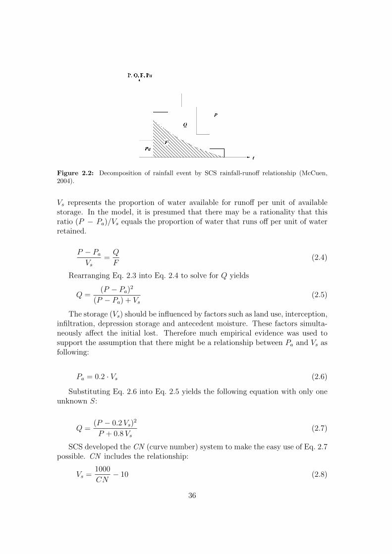
Figure 2.2: Decomposition of rainfall event by SCS rainfall-runoff relationship (McCuen,2004).

Vs represents the proportion of water available for runoff per unit of availablestorage. In the model, it is presumed that there may be a rationality that thisratio (P − Pa)/Vs equals the proportion of water that runs off per unit of waterretained.

P − Pa

Vs=Q

F(2.4)

Rearranging Eq. 2.3 into Eq. 2.4 to solve for Q yields

Q =(P − Pa)

2

(P − Pa) + Vs(2.5)

The storage (Vs) should be influenced by factors such as land use, interception,infiltration, depression storage and antecedent moisture. These factors simulta-neously affect the initial lost. Therefore much empirical evidence was used tosupport the assumption that there might be a relationship between Pa and Vs asfollowing:

Pa = 0.2 · Vs (2.6)

Substituting Eq. 2.6 into Eq. 2.5 yields the following equation with only oneunknown S:

Q =(P − 0.2Vs)

2

P + 0.8Vs(2.7)

SCS developed the CN (curve number) system to make the easy use of Eq. 2.7possible. CN includes the relationship:

Vs =1000

CN− 10 (2.8)

36

The SCS rainfall-runoff relationship has been used primarily for big naturalwatersheds. In the 1980s, SCS-TR 55, a variation of SCS was released with thenew adapted CN for urban areas.

Nevertheless, the suitability of the rational assumptions of Eq. 2.6 are stillquestionable, because of the assumption that the initial abstraction remains con-stant for the varying rainfall events in a given catchment. In other words, itshould not change with the intensity of the rainfall event. The equation solelysuggests that the soil surface includes a minimum storage capacity propor-tionalto total surface storage to hold rainwater back, independent of rainfall processes.In order to meet a reasonable assumption about surface runoff, a greater under-standing about the infiltration process is needed.

Nearly all infiltration equations suggest an infiltration rate with a rapid initialdecline and a final approach to a constant. Most equations are based on empiricalexperiments. The initial infiltration process is especially complicated and difficultto describe.

Horton’s Infiltration Model

Since the 1940s, possibly the best known and most widely used and process-basedmethod for computing infiltration and runoff is the “Horton’s infiltration model”,developed in 1937 (Eq. 2.9). His idea of storm runoff as an excess of rainfall overinfiltration capacity is called “Hortonian overland flow” or “infiltration excessoverland flow”. Horton used rainfall excess in short form. He strictly used theterm “infiltration capacity” instead of “infiltration rate”.

f = fc + (fo − fc) · e−k·t , (2.9)

where f = infiltration capacity [inches/hour] at time t [hour], fo = infiltrationcapacity at time t = 0; fc = minimum constant infiltration capacity; and k isconstant for a given curve (Beven, 2004).

The “Horton Infiltration Equation” has been employed to calculate runoffand infiltration for big natural watersheds, especially in combination with theunit-graph theory of LeRoy K. Sherman (1932) (McCuen, 2004). A numberof well-known hydrological simulation models make use of the Horton model inobtaining an assessment of infiltration and runoff rates (Green, 1986).

The impression has persisted that the Horton model is an empirical relation-ship because his equation sums up all processes affecting the rate of infiltrationcapacity change. However, the Horton Infiltration Equation results in a declinetowards a constant, which is similar to the pattern of change in infiltration ca-pacity in other equations such as Green and Ampt’s curve (Green and Ampt,1912) and Phillip’s curve (Philip, 1957b).

37

Philip’s Infiltration Model

By combining “Darcy’s law”

q = −K∂H

∂z(2.10)

and the “Continuity equation”

∂θ

∂t= −∂q

∂z, (2.11)

a general flow equation can be expressed as following:

∂θ

∂t= − ∂

∂z(K

∂ψ

∂z)− ∂K

∂z, (2.12)

where q = the flux which at the soil surface equals the infiltration rate, H =total hydraulic head which is the sum of the pressure head (Hp) and the gravityhead (Hg), K = the hydraulic conductivity, θ = the soil moisture, and t = time.Phillip solved Eq. 2.12 in a form of physically-based converging power series whichdescribes cumulative infiltration I as a function of time t (Philip, 1957a) and thensuggested a simplified formula for practical purposes (Philip, 1957b). Thus, thecumulative infiltration is

I = St1/2 + b · t (2.13)

and the infiltration rate is

i =∂I

∂t=

1

2St−1/2 + b (2.14)

The sorptivity S reflects the soil’s ability to absorb water by matrix forcesduring the initial stages of infiltration. b is essentially the saturated conductivityat which soil finally arrives after a long infiltration duration.

Rubin’s Experiments and Schwartzendruber’s Infiltration Model

Rubin (1966) implemented a fundamental research for the development of thetheory of water uptake during rainfall infiltration (also called rain-pond infiltra-tion). He divided the water uptake process into 3 infiltration sub-processes:

(i) non-ponding infiltration, involving rain not intense enough to produceponding;

(ii) pre-ponding infiltration due to rain that can produce ponding but thathas not yet done that;

(iii) and rain-pond infiltration, characterized by ponded water.

38

The first two processes are intensity-controlled and the latter is pressure-controlled, i.e. by the depth of water above soil surface. During non-pondinginfiltration, the soil surface has a limiting saturation moisture content specific tothe rainfall intensity, and the hydraulic conductivity gradually approaches therainfall intensity. During pre-ponding infiltration, the rain intensity exceeds theinfiltration rate, and the soil’s infiltration capacity is about to be reached.

In addition, he found that the decreasing infiltration flux curve under a con-stant rate of water application is not the same as that obtained when surfaceponding is imposed from t = 0 onward (Rubin, 1966). (In order to assure theabsence of hysteresis, a rainfall event was considered only if its intensity was anincreasing function of time. In my study the annual rainfall time series have tobe very precisely separated into rainfall events series so that the rainfalls withdecreasing intensity can be excluded.)

Schwartzendruber (1974) attempted to develop an empirical equation to de-scribe the intensity-dependent water uptake process investigated by Rubin (1966).He proposed the following mathematical description:

i = at−n + b , (2.15)

where i is infiltration rate, a and n are curve parameters specific to soil sur-face properties, and b is the saturated hydraulic conductivity. This was only animplicit expression of water uptake as a function of time, which includes bothseepage and surface storage filling. Nevertheless, based on this knowledge, hethen derived an equation to calculate the cumulative runoff under a constantrainfall flux (Swartzendruber and Hillel, 1975):

w = (r − b) · (T − T1) , (2.16)

where w is cumulative runoff, r is rainfall intensity, T is modified time, and T1is the modified time at which the surface storage Vs is ponded. He presumedthat there was a static depth of water V that could be stored on the surface ofthe infiltration plot before overflow would start to release any further cumulativewater excess as runoff from the plot. This static surface storage might exist evenon a smooth surface because sufficient water is needed to drive the cumulativerunoff from surface.

39

Part II

Materials and Method

40

Chapter 3

Developing the Paved WeighableLysimeter System

This chapter gives a detailed description about the weighable lysimeter systemwith permeably paved surface, and represents the most important stage in thiswork. It has been implemented for 2 years in Berlin, Germany. Our lysimeterswere developed to enable measurements

• of all components of the urban water budget,

• within a realistic walkway structure, and

• under completely natural hydrologic conditions.

It was essential that the system be able to

• measure the water budget components independently of each other,

• allow observation of the components correlatively with each other in a dy-namic process,

• ensure high mass and temporal resolution.

Using weighable lysimeters with permeably paved surfaces, the measurements ofrunoff generation, infiltration capacity, and evaporation performance have to beacquired continuously in time series for the whole experiment period. In addition,the measurement system has to be capable of determining the soil hydrologicalparameters such as surface storage and saturated hydraulic conductivity.

41

3.1 General Aspects of Lysimeters

Determination of the water budget components by lysime-ter

In general, a lysimeter system is used to acquire water budget components of topsoil zone. The acquisition takes place by weighing the amount of water movinginto and out of the system. According to the European definition, a lysimeteris a vessel container with local soil placed with its top flush and the groundsurface for the study of several phases of the hydrological cycle, e.g. infiltration,runoff, evapotranspiration, soluble constituents removed in drainage, etc (Diestelet al., 1993; DVWK, 1996; Fank et al., 2004; Berger and Cepuder, 2007; EuropeanLysimeter Plattform, 2008).

Seepage water can be sampled for detection of material flux within the soil.The lysimeter body is filled with original or artificial soils and its surface mustmatch the surrounding surface. The lysimeter surface can be free, planted orpaved. Large-capacity lysimeters can provide a realistic approximation of anysoil section for investigating the physical and chemical interactions taking placebetween atmosphere, pedosphere, and biosphere, observed under natural condi-tions. In Europe, there are 82 lysimeter stations and 40 of which are in Germany.Over 90 % of them are installed for studies of forestry, agriculture and disposalsites (Lanthaler, 2006).

A lysimeter measures the weight change of the lysimeter body. The sign ofthese values can express water inflows, like precipitation (P ), or water outflows,like evapotranspiration(ET ) in connection with other water budget components,like groundwater recharge (GW ) and runoff (RO).

Eq. 3.1 shows a common water balance equation in lysimeter:

P = RO +GW + ET + ∆W , (3.1)

where P = precipitation, RO = runoff, GW = groundwater recharge, ET =evapotranspiration, and ∆W = changable water storage. ∆W is calculated fromrearranging Eq. 3.1. During a precipitation event

∆W = P −RO −GW, (3.2)

if evaporation is likely negligible (ET = 0). In this case, ∆W gives the value ofincoming water infiltrating through paved soil surface.

During the dry period (P = 0 between precipitation events)

∆W = −ET −GW . (3.3)

In this case ∆W represents, with a negative value, the outgoing water evaporatingfrom the paved surface.

42

Problems

Little is known about weighable lysimeters with pavements. The ones used inthe past were for isolated studies, each aimed at addressing a unique aim, andan established system for manufacturing and using paved lysimeters has not yetbeen developed. From the reviews about lysimeter and water budget studies inSection 2.1, two significant problems can be brought out about the state of theart:

(i) In most water budget studies, infiltration was simply calculated as thedifference of precipitation and runoff without exact evaluation of infiltration ac-curacy through direct measurement. The evaporation was also computed by anempirical formula. Therefore, those studies could make a statement about theannual water balance or water balance of a certain water regime, but not a sophis-ticated statement about water budget processes. The reason is that estimation ofrunoff are more reliable, due to the high and simple accuracy of runoff measure-ment techniques, than those of infiltration, which is normally too complicated todetermine directly under real conditions.

(ii) Studies that attempted to include process-based observation (e.g. forrunoff dynamics) often employed the sprinkling tests in most cases. Sprinklingtests are suitable only for figuring out the peak discharges and runoff behaviorof storm events. The sprinkling technique has not gone so far as to exactlyreproduce small events that are frequently observed in reality. Thus, in order toconsider the varying water processes of small events, the experiment absolutelyneeds to be based on the given natural precipitation events.

Since the aim of this study is to accurately describe the surface water behavior,the following problems can arise for the experimental design:

• Lysimeter surface has to imitate all the characteristics of real urban soilsurfaces,

• Runoff delaying has to be avoided, and

• The neighborhood and boundary effects has to be avoided.

One remarkable characteristics of this study is that the experiment is runningin field conditions with paved soils that can match very closely to real urbansurfaces. Many experiments with strictly defined boundary conditions in lab-oratories could refer only to the runoff behavior of paving materials, but notthe runoff dynamics of paved soils, including seam materials. The experimentaldesign was strongly focused on enhancing the temporal resolution and avoidingunnecessary intermediate storage such as runoff delays within the gutter (calledgutter errors).

43

3.2 Measurement of the Water Budget Compo-

nents

3.2.1 Lysimeter Setup

In order to monitor every water budget phenomena a weighable lysimeter systemwith pavement was constructed in the field of UBA (Federal Agency for Envi-ronment) and installed in Berlin Marienfelde, in the southern part of Berlin (seeFig. 3.1).

Figure 3.1: Lysimeter location in Marienfelde, southern Berlin, Germany.

The lysimeter system consists of 2 paved lysimeters, 2 FAO reference lysime-ters (Fig. 3.2), and a climate station that existed already for the whole UBA field.The paved lysimeter, used here for studying the urban water budget, can measureall components of a water budget (precipitation, infiltration, evaporation, runoff,and groundwater recharge) separately. Infiltration is not only estimated as thedifference between precipitation and runoff, but can also be directly measured dueto the high resolution of lysimeter. Evaporation can also be directly determined.By using FAO lysimeters, the system is able to monitor the potential evapotran-spiration throughout the experiment. One rain gauge system is installed basedon the model of Hellmann (W.M.O., 2006). Further significant aspect of systemis the weighable runoff measurement set-up (see Chap. 4).

The lysimeter bodies stand in the basement where all actions are monitored(see Fig. 3.4). Fank et al. (2004) once suggested that the invisible lysimeter is the

44

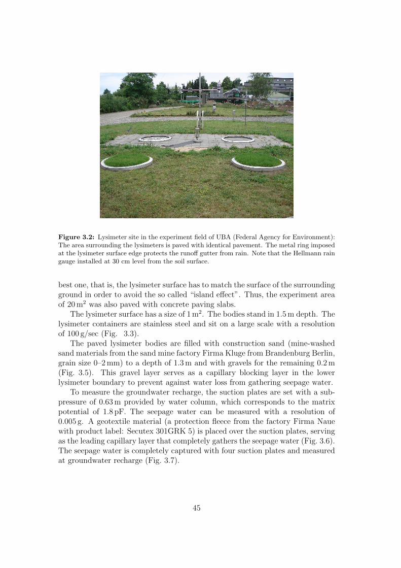
Figure 3.2: Lysimeter site in the experiment field of UBA (Federal Agency for Environment):The area surrounding the lysimeters is paved with identical pavement. The metal ring imposedat the lysimeter surface edge protects the runoff gutter from rain. Note that the Hellmann raingauge installed at 30 cm level from the soil surface.

best one, that is, the lysimeter surface has to match the surface of the surroundingground in order to avoid the so called “island effect”. Thus, the experiment areaof 20 m2 was also paved with concrete paving slabs.

The lysimeter surface has a size of 1 m2. The bodies stand in 1.5 m depth. Thelysimeter containers are stainless steel and sit on a large scale with a resolutionof 100 g/sec (Fig. 3.3).

The paved lysimeter bodies are filled with construction sand (mine-washedsand materials from the sand mine factory Firma Kluge from Brandenburg Berlin,grain size 0–2 mm) to a depth of 1.3 m and with gravels for the remaining 0.2 m(Fig. 3.5). This gravel layer serves as a capillary blocking layer in the lowerlysimeter boundary to prevent against water loss from gathering seepage water.

To measure the groundwater recharge, the suction plates are set with a sub-pressure of 0.63 m provided by water column, which corresponds to the matrixpotential of 1.8 pF. The seepage water can be measured with a resolution of0.005 g. A geotextile material (a protection fleece from the factory Firma Nauewith product label: Secutex 301GRK 5) is placed over the suction plates, servingas the leading capillary layer that completely gathers the seepage water (Fig. 3.6).The seepage water is completely captured with four suction plates and measuredat groundwater recharge (Fig. 3.7).

45

Figure 3.3: Scheme of paved weighable lysimeter.

46

Figure 3.4: Lysimeter basement.

Figure 3.5: Sand-bedding as pavement base.

47

Figure 3.6: Gathering seepage water at the lower boundary: Fleece material as capillaryconducting layer above the suction plates and the gravel layer.

Figure 3.7: Capillary blocking layer from gravel prevents the eventually ponded water atlysimeter bottom from rising up.

48

Figure 3.8: Water column and runoff discharge pipe: the water column provides suction plateswith a sub-pressure of ca. 63 hP. The runoff discharge pipe carries the runoff down from therunoff gutter.

49

3.2.2 Pavement Assembly with “Berlin’s Sidewalk”

The permeable pavement serves as materials for walkway, parking slots, sportsgrounds, streets, and roads with small burdening. In experiment, the walkwayvariation, so called “Berlin’s Walkway”, has been chosen, which consists of “Burn-burg mosaic cobblestones” and “Concrete paving slabs”. “Burnburg mosaic cob-blestones” is pavement with several natural stones from the region of a formermine in Bernburg, eastern Germany. The reason for this choice lies in the commonuse of these walkway materials in Berlin and many parts of Germany.

Fig. 3.9 presents lysimeter surface with “Bernburg mosaic cobblestone” and“Concrete paving slab”. These surrounding stainless steel rings protect the runoffgutter from collecting direct rainfall onto it. The pavement materials differ fromeach other in terms of the following properties:

(i) Concrete surface is normally much more porous than natural stones. Ac-cording to the studies of Wessolek and Facklam (1997), the porosity and fieldcapacity of cobblestone are 3.9 Vol.% and less than 0.5 Vol.%, respectively, whilethose for concrete are 5.1 Vol.% and 1.0 Vol.%.

(ii) The seam portion of cobblestone pavements is normally much biggerthan that of concrete pavements. In terms of heat and temperature behavior,pavements show very different daily fluctuations depending on the seam portion(Starke, 2011; Wessolek and Facklam, 1997).

For calculating the seam portion, Rim (2008) suggested a procedure. Thisprocedure yields the seam portion of max. 45 % for pavements from Bernburgermosaic cobblestone (MCS) and max. 10 % for pavement from concrete pavingslabs (CPS).

The upper surface and sub-base of lysimeter pavements attempt to imitatethe actual streets of Berlin. Each lysimeter has a a slope of about 2 % from themiddle point to surface border. In real urban conditions the common gradientfor road construction is between 1 % and 5 %. Due to practical reasons and thebest construction practices, the gradient of 2 % was here chosen (Niesel, 2002).

In Fig. 2.1 an example of the standard vertical structure of a street andwalkway is shown. In this work, no such sub-base structure was used for thefollowing reasons:

(i) the new seam materials decline somehow in porosity after extended use(Borgwardt et al., 2000) and reach a clogging -state quickly;

(ii) in practice, a sub-base is commonly not needed in the construction ofwalkways, and the walkway is instead bedded directly in base sand by a vibratoryplate machine; and

(iii) well-structured sub-bases with high retention capacity do occur, but areevidenced not to increase surface evaporation considerably (Starke, 2010).

50

(a) Bernburg mosaic cobblestones (MCS).

(b) Concrete paving slabs (CPS).

Figure 3.9: Lysimeter surface with the materials of “Berlin’s Walkway”.

51

Table 3.1: Parameter of lysimeter pavements. Almost identical seam material and sub-basestructure are used for both pavements of Bernburg cobblestone and concrete paving slabs. Thesurfaces differ rather due to the surface properties like seam portion and pavement size. Theseam materials were collected from different sites in Berlin.

layer Properties Bernburg mosaic cobblestone

Concrete paving slabs

seam portion [%] 40 7surface slope [%] 2 2

size [cm•cm•cm] min. 4 • 4 • 4max. 6 • 6 • 6 30 • 30 • 4

seam width [mm] 5 - 10 2 - 7thickness [mm]ρB [103g/cm3]

sand [%] 89.68* / 86.27 **

silt [%] 8.39* / 12.73 **

clay [%] 1.98* / 1.00 **

humus [%]thickness [mm]ρB [103g/cm3]

sand [%]silt [%]

clay [%]humus [%]

ρB [103g/cm3]sand [%]

ρB:dry bulk density,* by Wessolek and Facklam (1997), ** by Nehls et al (2006)100

Seam material(0 - 1 cm)

2.88

1.51Base material ( > 5 cm)

95.23**

4.37**

0.43**

0.37**

Sub-base material(1 - 5 cm)

1.61**

Paving material

1.49**

10

40

52

3.2.3 General Runoff Assembly

Throughout the study, runoff measurement will be the key method for measuringchanges in the water balance. In general, the runoff process for paved catchmentareas consists of runoff generation at the surface and runoff transport along theflow path. According to the complexity of soil and surface flow path properties,both processes will shape a causal relationship that is known as “runoff concen-tration”. Here, the runoff generation process considerably influences the runofftransport process.

Two rainfall-runoff relationships are of great interest:(i) the total runoff depth and(ii) the runoff peak discharge.

The first relationship is primarily dependent on the infiltration capacity of thecatchment surface, while the latter is additionally dependent on the concentrationprocess. The smaller the catchment surface size is, the more clearly the runoffgeneration can be observed.

Hence, owing to the small area of the lysimeter surface (1 m2), the observedrunoff process presumably represents the runoff generation process. The above-mentioned runoff depth and the peak discharge can be described in high accuracy.Therefore, lysimeter surface can be defined as a “representative elementary sur-face”.

As the runoff from the paved surface at the beginning of a rainfall event pro-ceeds in interplay with the initial infiltration of short duration, a good temporalresolution is important. For this reason, our weighable lysimeter can provide theoption to precisely monitor the initial infiltration process. Further, the evapo-ration of short duration that follows immediately after the rainfall event can bepersued in a high timely manner.

In Fig. 3.10, seam material is being compressed by pouring water onto it inorder to consolidate the soil surface without using a vibratory plate machine.In this figure the produced runoff is streaming downwards to the runoff gutter,which is set up directly along the surface edge. This allows the run-off to beimmediately shunted to a separate discharge pipe.

Fig. 3.11 illustrates the runoff collection process through the runoff gutter.The collected runoff water goes to the tipping bucket, which be used to canquantify the unit volume of water.

No water is lost in this procedure. The lysimeter wall and drain gutter aremade of high-grade stainless steel. . The amount of runoff water that is retainedin the gutter is called the runoff gutter error. In our system it amounts to max.150 ml that corresponds to 0.15 mm and the delaying time span is not more than10 minutes (see Chap. 5.1).

53

Figure 3.10: Water pouring to consolidate the seam material and runoff water flowing torunoff gutter. The runoff gutter is fixed along the lysimeter side wall.

Figure 3.11: The upper surface (at least the top 1 cm) of pavement is the most altered andcompressed soil in real urban streets. The soil zone of next 4 cm below that is less compressed.Runoff water is collected in the runoff gutter and flows to the runoff tipping bucket in thelysimeter basement.

54

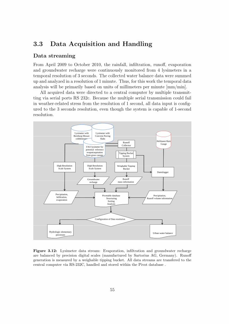
3.3 Data Acquisition and Handling

Data streaming

From April 2009 to October 2010, the rainfall, infiltration, runoff, evaporationand groundwater recharge were continuously monitored from 4 lysimeters in atemporal resolution of 3 seconds. The collected water balance data were summedup and analyzed in a resolution of 1 minute. Thus, for this work the temporal dataanalysis will be primarily based on units of millimeters per minute [mm/min].

All acquired data were directed to a central computer by multiple transmit-ting via serial ports RS 232c. Because the multiple serial transmission could failin weather-related stress from the resolution of 1 second, all data input is config-ured to the 3 seconds resolution, even though the system is capable of 1-secondresolution.

Lysimeter with Bernburg Mosaic

Lysimeter with Concrete PavingBernburg Mosaic

cobblestonesHellmann Rain

GaugeRunoff CollectorFAO lysimeter for

potential reference

Concrete Paving Slabs

Weighable TippingHigh Resolution

evapotraspirationfrom grass canopy

Tipping Bucket System

High Resolution Weighable TippingBucket

Runoff

Datenlogger

High Resolution Scale System

High Resolution Scale System

Groundwater

Pivottable database

mass information

Precipitation, Precipitation

recharge

Pivottable databaseStructuring

SortingAnalysis

Infiltration,evaporation

Precipitation,Runoff volume information

Configuration of Data resolution

Hydrologic elementary processes

Urban water balance

Figure 3.12: Lysimeter data stream: Evaporation, infiltration and groundwater rechargeare balanced by precision digital scales (manufactured by Sartorius AG, Germany). Runoffgeneration is measured by a weighable tipping bucket. All data streams are transfered to thecentral computer via RS-232C, handled and stored within the Pivot database .

55

Scales and Equipments

In the experiment, a complex system of balancing equipments was needed tomeasure all water budget components separately. Precipitation amounts weredetermined primarily with the Hellmann rain gauge (W.M.O., 2006), which worksalong with the embedded precision tipping equipment (often called the tippingbucket). Lysimeters are theoretically also able to measure the precipitation depthaccording to an objective target, too. Here, the precipitation data determinedby lysimeter were used as controlling data for the data correctness as gauged bythe Hellman model when suspected data errors happeneds to arise.

The employed Hellmann gauge counts a unit volume each time the fallingrain fills the tipping bucket. This unit volume is the volumetric amount of waterthat the tipping bucket releases by changing its position. The Hellmann gaugeused has a 200 cm2 apparatus surface and a tipping volume corresponds to 2 ml,allowing a measurement resolution of 0.1 mm (equals to = 0.002 L/0.02 m2) (seeFig. 3.13).

The tipping signal is registered in a Combilog 1020 (data logger for Hellmanngauger and runoff gutter). The Combilog 1020 is able to register and processthe series of tipping signals with its own CPU. This runs continuously with itsown battery. By this device the automatic measurement is ensured even in badweather situations.

Similarly, the runoff measurements were also made using a tipping-based vol-ume scale (tipping bucket). The runoff tipping bucket used (manufacturer: UMSGmbH, Germany, 2006) has a unit tipping volume of 100 ml. As the lysimetersurface surface area is 1 m2, the runoff measurement resolution also comes to0.1 mm (equal to 0.1 L/1 m2). Fig. 3.8 and Fig. 4.2 show the introduced tippingbucket subjected to a runoff system..

Using a tipping bucket, an exact value of water mass can normally be gained.The disadvantage is the undefinable temporal resolution. The bigger the tippingvolume becomes, the more often this problem. In the case of the runoff tippingbucket in our system, the low temporal resolution can give an misleading state-ment about time-related runoff processes. Many small events can get lost withoutbeing included in sample groups if the runoff water was less than one tipping vol-ume (100 ml). To handle this problem, we developed an improved setup called aweighable tipping bucket (WTB).

A WTB is a combination of a normal digital scale and tipping equipmentconnected through a trasit lever. A WTB demonstrates a mass resolution of0.0005 mm by doubling the 1 g step of scale with lever structure. In the Chap. 4more is discussed about WTB.

As for the lysimeter balance, a huge industrial balance was used which canfunctionally hold the entire weight of ca. 8000 kg from sand and water. Nev-ertheless, the precipitation, infiltration and evaporation could be measured verysufficiently with resolution of 0.1 mm. This resolution is the ratio of the balance

56

Figure 3.13: Hellmann gauge in 30 cm level from the paved surface in lysimeter station.

resolution to surface area (equal to 100 g/1 m2. In contrast to the tipping bucket,the lysimeter balance can theoretically demonstrate weight value in 1-second in-tervals. A sensitive lever of the lysimeter balance is equipped with a metal rod,which transmits the mechanical movement due to weight change towards a precisedigital scale.

The seepage water, gathered by the suction plates and capillary conductinglayer, arrives at the seepage water container through the water column. The dig-ital scale for measurement of groundwater recharge can give groundwater weightvalues at a resolution of 0.005 mm.

Data Handling

The central monitoring computer manages a data base that allows

• automatic structuring, sorting and navigating;

• automatic event separation and analysis; and

• real-time axis dimension.

For data handling, tools like Labview, Visual-Basic, and PIVOT table databasewere used (Jamal and Hagenstedt, 2004; Schwenk and Schuster, 2009). Usingthe visual programming software Labview, the ten RS 232C ports were scannedthrough every 3 seconds. The Visual-Basic (VBA) algorithm mainly recomposes

57

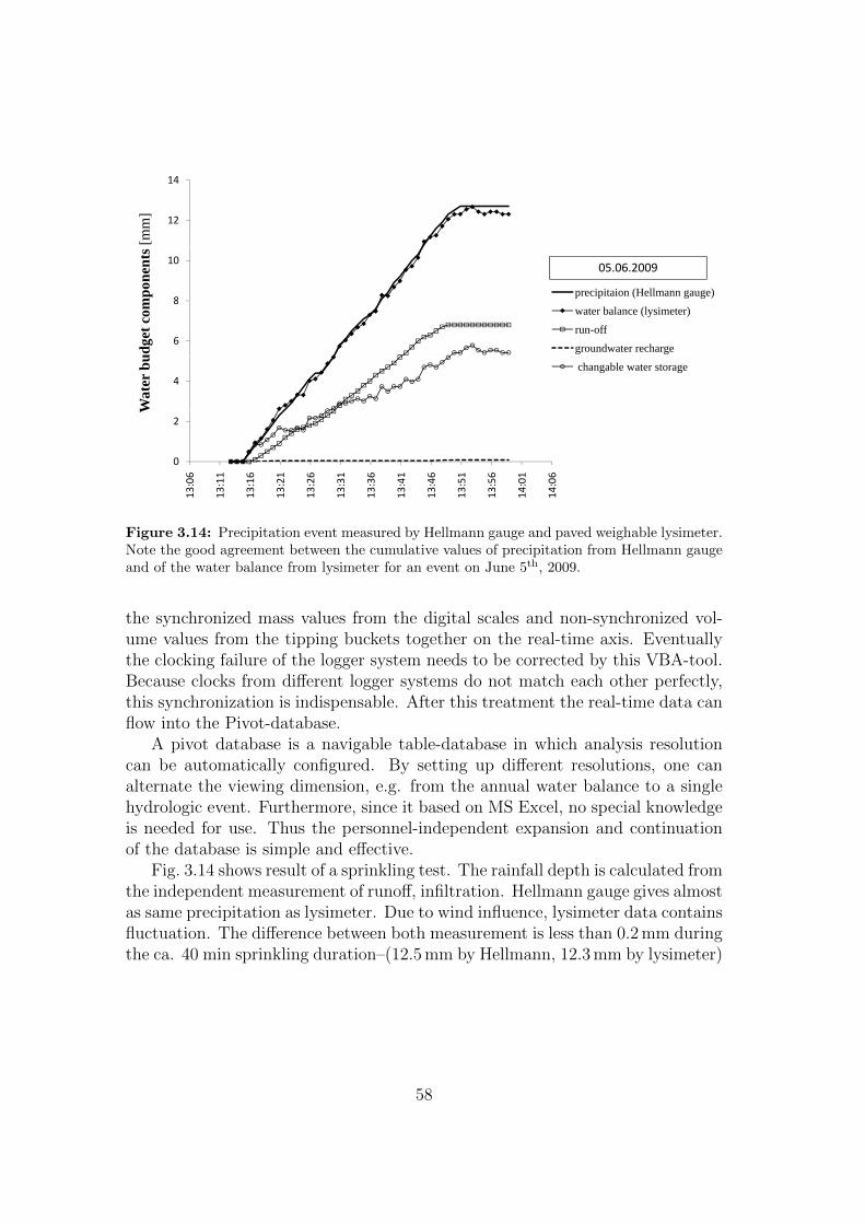
14

12

[mm

]

8

10

mpo

nent

s

precipitaion (Hellmann gauge)

05.06.2009

6

8

udge

t com water balance (lysimeter)

run-offgroundwater recharge

4

Wat

er b

u

changable water storage

0

2

W

13:06

13:11

13:16

13:21

13:26

13:31

13:36

13:41

13:46

13:51

13:56

14:01

14:06

Figure 3.14: Precipitation event measured by Hellmann gauge and paved weighable lysimeter.Note the good agreement between the cumulative values of precipitation from Hellmann gaugeand of the water balance from lysimeter for an event on June 5th, 2009.

the synchronized mass values from the digital scales and non-synchronized vol-ume values from the tipping buckets together on the real-time axis. Eventuallythe clocking failure of the logger system needs to be corrected by this VBA-tool.Because clocks from different logger systems do not match each other perfectly,this synchronization is indispensable. After this treatment the real-time data canflow into the Pivot-database.

A pivot database is a navigable table-database in which analysis resolutioncan be automatically configured. By setting up different resolutions, one canalternate the viewing dimension, e.g. from the annual water balance to a singlehydrologic event. Furthermore, since it based on MS Excel, no special knowledgeis needed for use. Thus the personnel-independent expansion and continuationof the database is simple and effective.

Fig. 3.14 shows result of a sprinkling test. The rainfall depth is calculated fromthe independent measurement of runoff, infiltration. Hellmann gauge gives almostas same precipitation as lysimeter. Due to wind influence, lysimeter data containsfluctuation. The difference between both measurement is less than 0.2 mm duringthe ca. 40 min sprinkling duration–(12.5 mm by Hellmann, 12.3 mm by lysimeter)

58

Chapter 4

A New Technical Approach forMeasuringthe Runoff Dynamics

The high temporal and quantitative resolution of runoff measurement is of sig-nificant interest. In this study, a runoff setup was installed with a runoff gutter,discharge pipe, and tipping bucket (TB). The common tipping buckets have agood volumetric accuracy in volume resolution and are capable of quantifying thehighest rainfall intensities over a range of expected flows. However, this leads tothe varying temporal resolutions for different flow intensities, and in particularresults in low resolutions for small flow events. Therefore, their applicability torunoff measurements and other hydrological process studies is limited, especiallywhen the dynamics of both small and large flow events will be described.

To solve this problem, an improved technique for runoff dynamics was addedto the TB. It is accomplished by coupling the TB to a digital balance, called aweighable tipping bucket (WTB). The improved volume and temporal resolutionof the WTB and the associated data processing concepts are demonstrated. Asystematic uncertainty of TB measurements compared to WTB measurements iscalculated. The impact of the increased resolution on our understanding of runoffdynamics on paved urban soils are discussed, exemplary for the runoff and theinitial loss of a paved urban soil.

4.1 General Aspects of Runoff Measurements

The dynamics of the urban water balance are not completely understood (Ragabet al., 2003). Measuring runoff from permeable paved urban soils in a hightemporal and quantitative resolution is the prerequisite for the formulation ofa process-based surface water model. Such a model, based on meteorologicaldata and pavement characteristics, would be capable of predicting changeable

59

runoff behavior for the changing rain volume and intensity distribution due toclimate change as forecasted (Arnbjerg-Nielsen, 2006). Such models are thereforeof interest for the development of climate change adaptation strategies for urbanareas, such as drainage adjustment (Arnbjerg-Nielsen and Fleischer, 2009; Faramet al., 2010), the use of runoff water as an urban cooling resource for improvedevapotranspiration (Nakayama and Fujita, 2010) or risk assessment for increasedinfiltration (Gobel et al., 2007; Nehls et al., 2007).

Importance of small events In this study, the water balance of pavementsis measured using 1 m2 weighable lysimeters (Rim et al., 2009). On the lysimetersurfaces, small rain events lead to small absolute runoff flows. However, thesehave to be detected. For understanding the processes that influence runoff gen-eration from paved soil surfaces, small rain events are of the same or even greaterimportance than storm events for two reasons:

(i) Figure 4.1 demonstrates the long-term precipitation event sum distribu-tion. It highlights the contribution of small precipitation events to the cumula-tive sum of precipitation in the study area. Similarly, precipitation events withsmall intensities contribute substantially to the total sum of precipitation (seeChap. 5.2). At the station Berlin-Marienfelde, 5 %, 50 % and 95 % of the cumula-tive rainfall is generated by rain fall events with intensities smaller than 0.0076,0.0263 and 0.1886 mm/min respectively.

(ii) The runoff (RO) is a non-linear function of precipitation sum (P) andintensity (Sen and Altunkaynak, 2006). This means that different runoff gener-ation processes might be of differing effectiveness for different rainfall amountsand intensities. Therefore, one needs to study runoff for both small and heavyrainfall events.

The functional principle of a TB is to count how often the two buckets withknown unit tipping volume are filled and self-emptied. This principle has beenused since the 1950s and is often used in hydro-meteorological instrumentationsuch as rain gauges (W.M.O., 2006) or stem flow meters (White and Rhodes,1970). Tipping buckets have also been regularly employed for runoff measure-ments since the early 1960s (Pillsbury et al., 1962; Edwards et al., 1974; Khanand Ong, 1997). In addition, they are, used in wick samplers and lysimetersfor the measurement and sampling of seepage water and for multi-compartmentsampling (Meissner et al., 2010).

TBs are robust, reasonably-priced devices for the discontinuous detection offlow events with a wide spectrum of flow intensities and a high temporal res-olution at the flow intensities for which the bucket was dimensioned (Habib et al.,2001). During instrumentation of our lysimeters, we became aware that thetraditional TB is not appropriate for providing constant measurements, at hightemporal and volumetric resolution, of runoff with both very low and very highflow intensities. Below is an explanation of why it is not suitable as it is and how

60

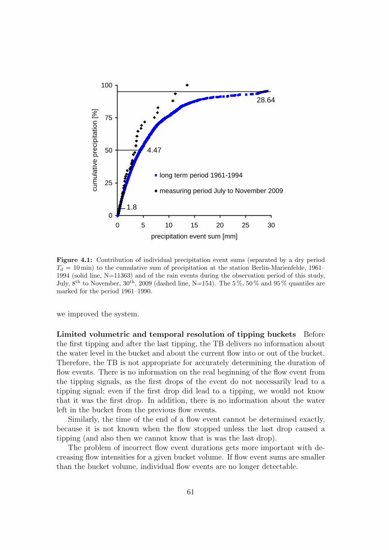
0

25

50

75

100

0 5 10 15 20 25 30

precipitation event sum [mm]

cum

ulat

ive

prec

ipita

tion

[%]

long term period 1961-1994

measuring period July to November 2009

1.8

4.47

28.64

Figure 4.1: Contribution of individual precipitation event sums (separated by a dry periodTd = 10 min) to the cumulative sum of precipitation at the station Berlin-Marienfelde, 1961–1994 (solid line, N=11363) and of the rain events during the observation period of this study,July, 8th to November, 30th, 2009 (dashed line, N=154). The 5 %, 50 % and 95 % quantiles aremarked for the period 1961–1990.

we improved the system.

Limited volumetric and temporal resolution of tipping buckets Beforethe first tipping and after the last tipping, the TB delivers no information aboutthe water level in the bucket and about the current flow into or out of the bucket.Therefore, the TB is not appropriate for accurately determining the duration offlow events. There is no information on the real beginning of the flow event fromthe tipping signals, as the first drops of the event do not necessarily lead to atipping signal; even if the first drop did lead to a tipping, we would not knowthat it was the first drop. In addition, there is no information about the waterleft in the bucket from the previous flow events.

Similarly, the time of the end of a flow event cannot be determined exactly,because it is not known when the flow stopped unless the last drop caused atipping (and also then we cannot know that is was the last drop).

The problem of incorrect flow event durations gets more important with de-creasing flow intensities for a given bucket volume. If flow event sums are smallerthan the bucket volume, individual flow events are no longer detectable.

61

The starting point of a flow event can be extrapolated from the behavior ofthe flow during the reliable TB measuring period, especially when the rise of theflow intensity at the beginning of the event is very steep. However, this is alreadyan interpretation of measured data and not a true measurement.

The TBs are usually dimensioned to detect the highest of an expected rangeof flow intensities. This is done by choosing the bucket size according to theexpected flow rate and the maximum possible tipping frequency. Then, TBsprovide proper information, especially during high flow events, after the firsttipping and before the last tipping of the buckets. This duration is the “reliableTB measurement period”.

Because of the distinct volume of the bucket, low flow intensities lead to lowtemporal resolutions, and high flow intensities lead to high temporal resolutions.The problem of the resulting high measurement uncertainties is discussed by Yuet al. (1997). If, as in this study, a wide range of flow intensities are of the sameinterest as great events, TBs are inappropriate measuring devices in terms oftemporal resolution.

Further, different flow events cannot be detected with an adequate, a priorichosen temporal resolution. This is a disadvantage of the TBs concerning theharmonization of measurements of different water balance elements in the samecatchment. The bucket volume could be decreased to increase the resolution forsmall events, but that would decrease the maximum detectable flow rate of theTB. Also, the filling of the bucket needs to take a sufficiently long time comparedto the duration of a complete tipping (Yu et al., 1997). Otherwise, the TBoverflows without quantification of the flow.

It can be argued that the water balance for the TB itself is closed over longperiods. Water that is left in the bucket after an event will be added to the nextevent. Using this argument, TBs have been employed for runoff studies aimed atthe measurement of annual mean runoff amounts for paved urban soils (Wessolekand Facklam, 1997; Wessolek, 2008). However, for systems in which the tippingbucket cannot be sealed against the atmosphere, as in our setup, water could belost from the bucket due to evaporation. Even small evaporated amounts maythen sum up to substantial losses at the end of the observation period.

The traditional TB had to be improved to be applicable for our studies ofrunoff generation and runoff dynamics from paved urban soils. The volume res-olution given by the bucket size of the TB had to be improved substantially,without decreasing the capacity to detect high flow events. By increasing thevolume resolution of the TB, we were able to also increase its temporal resolu-tion.

62

Figure 4.2: Scheme of the weighable tipping bucket system. The blue arrow indicates the waythe water has to go when leaving a) the tipping bucket and b) the box. The other parts of theset-up are c) the lever connected to the balance by a screw, d) the balance and e) the pivot.

4.2 Weighable Tipping Bucket

WTB Setup

In the lysimeter basement, runoff water is collected by a tipping bucket (Pulsame-ter MC 1, UP Umweltanalytische Produkte GmbH, Cottbus, Germany) with abucket volume of 0.1 L which is equivalent to 0.1 mm of runoff from the pavedsurface. During calibration, the average of the two bucket volumes (VB) wasmeasured as 0.098 L (standard error = 0.002 L).

The TB has been coupled to a digital balance (Acculab VIC-4KG, SartoriusAG, Goettingen, Germany) with a resolution of 1 g. The TB is mounted at theend of a lever with the length l1, which is pivoted at the another end (Fig. 4.2).This leverage construction was needed in order to discharge the TB withoutmaking the digital balance wet. At the distance l2 = 0.51× l1, a screw transmitsthe force to the digital balance. The distance l2 was estimated during calibrationof the balance system using 100 g test weights. The calibration of the balancehas been repeated at the end of the measuring period. The drift of the balancewas lower than 1 g. However, we enhanced twice the resolution of the balance atits detection limit.

The screw connects the balance to the leverage and allows the TB to adjusthorizontally, which is a prerequisite for the proper functioning of the TB. Due tothe leverage effect, the accuracy of the WTB system as a whole is Vmin ≈ 0.001 L.

63

The signals from both the TB and the WTB are recorded by data loggers (seeChap. 3.3). The temporal resolution of the TB varies with the runoff intensity;the maximum flow intensity detectable by the TB is 15 mm/min. Due to sometechnical reasons described above, in this study the temporal resolution of thedata logger connected to the balance is 3 s.

Data Processing Concept

To correct the leverage effect, the weights detected by the digital balance weremultiplied by the factor 0.5 in order to get the actual water weight in the tippingbucket. The TB signals were processed as follows: the first tipping is accountedfor as 0.5 VB, every following tipping is accounted for as VB. After the last tipping,another 0.5 VB is added to the sum of tippings before. This evenly distributes thewater left in the bucket after the last tipping of an event and the water collectedbefore the first tipping of the subsequent event to all of the individual events.

The sum of a runoff event measured by the TB is therefore

ROTB =nVBA

(n ∈ N) [mm] , (4.1)

where n = the number of tippings, VB = the bucket volume [L] and A [m2] =the paved surface area.

The WTB data was processed as follows: the volume of water collected beforethe first tipping (VFT) was calculated as difference between the volume beforethe beginning of runoff and the highest volume detected. The volume of watercollected after the last tipping of an event (VLT) is calculated as the differencebetween the lowest volume of the tipping bucket and the volume at the end ofthe event.

The beginning of an event is identified as follows: if the previous runoff hascompletely finished, it is simply the first positive weight change of the balanceafter a long period of no changes or decreasing weights due to evaporation. If thesubsequent rain event is over, but the runoff is still being collected, the two rainevents and the associating runoff events cannot be separated and are processedas one event.

When the rain event is over and the runoff from the surface has also stopped,the WTB can still collect water. Such water is the draining of the gutter systemthan runoff. The runoff detection is delayed due to the measurement set up. Acriterion is needed to identify the end of real surface runoff. Based on observa-tions at our lysimeter, this criterion has been chosen to be a flow rate less than0.002 L/min. Such draining water is still accounted for as runoff, but is no longeraccounted in terms of runoff duration (Fig. 4.3).

After the first tipping, every tipping is accounted with VB [L]. The sum of therunoff event measured by the WTB is therefore

64

ROWTB =

VFT

Afor n = 0

(n− 1)VB + VFT + VLT

Afor n ≥ 1, n ∈ N

[mm] (4.2)

where VFT [L] = the volume of water collected before the first tipping andVLT [L] = the volume of water collected after the last tipping of an event.

The runoff sum for the observation period was calculated as the sum of theindividual events both for TB and WTB data according to equations 4.1 and 4.2.The surface storage VS was estimated by the maximum rain event sum, at whichno runoff was detected, both using TB and WTB data.

4.3 Increased Accuracy of Surface Runoff

Measurement using WTB

Increased volume resolution

The runoff generation from the permeably paved lysimeter surface was studiedusing and comparing the data gained from the TB and the WTB. For example,one single runoff event on the 3rd of September 2009 is shown in Fig. 4.3. Thisrain event started at 10:42 lasted for 33 min and had a sum of 1.2 mm. For thisRO event, the TB tipped five times, and a runoff of 0.5 mm and 0.45 mm wasdetected by the TB and the WTB ,respectively. Note that from 10:43 until 11:03a total of 0.004 L entered the WTB. This water was left in the gutter systemfrom the previous rain event, which ended 9:45 and was also accounted to thesubsequent RO event.

The absolute difference ROWTB − ROTB is -0.05 mm. The relative differenceU (Eq. 4.3) is -10 %, while the maximum difference would be -17 % (see Eq. 4.4).

This example underscores the great advantage of the WTB system and givesan impression of the reliability of measurements made using solely the TB.

As shown in Fig. 4.3, the weights for the maximum filled and the emptybuckets vary. This might be due to differing volumes for the left and the rightbuckets, as this was estimated during calibration of the system. While the leftbucket volume is 0.1029 L, the right bucket only fills up to 0.0955 L before tipping,resulting in a VB of 0.0987 L.

However, this effect is not the only reason for the difference, as the volumesof water at tipping are not reproducible. Further effects are responsible:

(i) water needs some time to flow out of the TB box, which is indicated inFig. 4.2. In the meantime, water enters the TB box from above. Thus, theWTB detects water entering and leaving the TB box in the same time step.The resulting uncertainty is proportional to the flow intensity. Consequently, the

65

balance detected the lowest weight for the empty bucket and one of the highestweights for the full bucket, when the flow intensity was the smallest at the endof the runoff event shown in Fig. 4.3 and Fig. 4.4.

(ii) The different maximum and minimum bucket weights are also an artifactof the 3 s measuring interval of the balance. For the runoff event at the 3rd ofSeptember 2009 mentioned above, we calculated a flow rate of 3.3·10−3L for theinterval between the first and the second tipping of the TB. That results in anuncertainty of ca. 0.01 L for the maximum and minimum filling of the TB at thisflow rate and the given temporal resolution of the digital balance.

Because of (i) and (ii), the runoff is calculated from the tipping signals insteadof the balance data between the first and the last tipping of the bucket (seeEq. 4.2).

Furthermore, (iii) the buckets of the TB spin along the leverage and notperpendicular to it. For technical reasons in our individual case, it was notpossible to mount the tipping bucket in a different way. This means that thesimilarly filled buckets would lead to different weights detected by the balance dueto the different torques. The two buckets have the following leverage factors: 0.50for the shorter lever and 0.52 for the longer lever. However, the bucket volumeswere calculated using the average factor of 0.51 for the first approximation.

Systematic uncertainty of TB compared to WTB

While the discrepancy between runoff measurement by TB and WTB can behigh for a single event, it will be smaller after a long observation period with ahigh number of tippings, as then the relative contribution of the first and the lasttippings to the sum of tippings decreases.

In the following description, the maximum relative difference between WTBand TB (Umax) for a certain number of tippings of TB is calculated. We considerthe WTB data to be more precise than the TB data for the following reasons:the WTB system uses the same tipping information as the TB but also deliversinformation about the water flow in periods between two tippings. In this periodthe WTB has a volumetric resolution 200 times higher than that of the TB.A testing of the assumption of the higher precision of the WTB in a physicalexperiment is not truly possible, because the device can only compared to itself.First, the device is compared to exactly itself. Any test of the weighing functionof the WTB must be based on the quantification of a water flow, which wouldonly be possible with another balance. In such a test, one balance would just becompared to another balance. Because measuring the weight is one of the basicphysical measurements, and because we employed a calibrated digital balance forthe measurement of the mass of the TB, we assume that the weight of the TB ismeasured as precisely as described above.

The relative detection limit of the digital balance compared to the bucket (x)can be expressed as x = Vmin/VB. With Vmin = 0.001L and VB = 0.1L x equals

66

0.01.Generally, ROWTB can be higher or lower than ROTB, leading to positive or

negative differences. In the case of the maximum positive difference, ROWTB −ROTB, the bucket is almost empty (= 0.001 L) at the beginning of the event andis left almost filled (= 0.099 L) at the end (then, Umax → max for (VFT + VLT)→2(VB − xVB)). In case of the maximum negative difference, the bucket is almostfull at the beginning of the event (= 0.099 L) but left almost empty (= 0.001 L)at the end (then, Umax → min for (VFT + VLT)→ 2xVB).

Substituting

Umax =ROWTB −ROTB

ROWTB

× 100 % (4.3)

with Eqs. 4.1 and 4.2 for VFT + VLT → 2xVB and VFT + VLT → 2(VB − xVB)reveals

−1 + 2x

n− 1 + 2x× 100 % ≤ Umax ≤

1− 2x

n+ 1− 2x× 100 % (4.4)

From Eq. 4.4 one can learn that the maximum systematic uncertainty is high-est for small runoff volumes leading to no or only a small number of tippings.|Umax| is lower than 5 % and 1 % for 21 and 99 tippings, respectively, which equalsa run off of 2.1 mm and 9.8 mm. The rain distribution in Fig. 4.1 demonstratesthat uncertainties higher than 5 % must be assumed at least for 28 % of all rainevents (assuming a linear RC of 1) when a TB is used for measurements. How-ever, we know that RC is not linear for different rain intensities and that dueto evaporation of rain water from the surface and infiltration, higher maximumsystematic uncertainties must be assumed for the quantiles mentioned above.

Increased temporal resolution

Employing WTBs instead of TBs increases the temporal resolution of the runoffobservation. The rain event on September, 3rd, 2009 started at 10:42 am, lastedfor 33 min and and resulted in a total of 1.2 mm (Fig. 4.3). The associated runoffevent lasted from 11:03:01 am until 11:33 am as detected by the WTB, but onlyfrom 11:03:13 am until 11:13 am as detected by the TB (Fig. 4.4).

Depending on the water level in the bucket, the starting times of runoff eventsdetected by TB and WTB might be close. This is due to the steep increase ofthe runoff intensity at the beginning of the event. At the end of the runoff event,the flow intensity tails out slowly. From the TB data, the runoff appears to havealready stopped before the end of the rain. That scenario is not impossible: itcould be explained by processes like evaporation or infiltration. The low volumeresolution of the TB system leads to a very low temporal resolution. In contrast,

67

the WTB can detect the end of the runoff event much better due to its increasedvolume resolution and the constant high temporal resolution.

This has important consequences for the measurement of runoff dynamics, e.g.the runoff concentration time (tc). When measuring with the TB, for a given rainintensity and a given moisture content in the pavement, tc depends on pavementcharacteristics such as VS, rain intensity and other climatic conditions, but alsoon the level of water in the bucket, left over from the last event. Measuringwith the WTB, in contrast, detects a tc which is almost solely dependent on thepavement, rain intensity and climatic characteristics.

Accuracy of Runoff for a Test Period

During the observation period, 8th of July until 1st of December 2009, the TBdetected a total of 71.6 mm of runoff, while the WTB detected 79.6 mm. Thisdifference is equal to 11 % of the total runoff detected by the TB. Up to 95 % ofthe difference can be explained by evaporation losses from the TB. During themeasurement period, a quantity of 7.6 L evaporated from the TB, as calculatedfrom weight losses from WTB in the periods between the runoff events.

In this study, the individual runoff events, especially those caused by smallrain events, were of interest rather than the sum of runoff over a long period.During the observation period, the rainfall gauge detected 154 rainfall events,leading to 121 and 47 runoff events, detected by the WTB and TB respectively.The higher resolution of the WTB compared to the TB led to more observationsand will lead to a different description of runoff processes.

This is shown by the following example: although the runoff coefficient (RC)is not constant for different precipitation events, one can calculate an averagerunoff coefficient (RC) and its standard deviation (SD) for the detected runoffevents, in order to compare the data sets: for events detected by the TB, RCTB

is 0.38 (SD = 0.21, N=47), while for events detected by WTB RCWTB is only 0.10(SD = 0.23, N = 121). Using TB data would overestimate the runoff formationcompared to WTB data. Additionally, WTB data has higher variation than TBdata; thus the first delivers more comprehensive information for process studiesthan the latter.

Accuracy of Initial Loss from Runoff Measurements

As not all rain events lead to runoff, there must be a retainment of water on orin the pavements. It is not the goal of this work to study this topic in detail, butwe can show that the magnitude of VS measurements strongly depends on thevolume resolution of the measuring device.

According to our hypothesis, the storage VS is the sum of free water retainedat the surface of pavements in its micro relief (VR), the air-filled pore volume of

68

porous pavements (VP) and the air filled pore volume of the seam material andthe underlying soil VSM:

VS = VR + VP + VSM [mm] (4.5)

VS is a function of the initial water content and the material and designcharacteristics of the pavements and the pavement system, as well as a functionof the pore system properties of seam material and the underlying soil. Firstestimations of the maximum VSmax can be derived from the maximum rain eventswhich did not lead to runoff. Analyzing the TB data, VSmax is then 2.5 mm, butthis value is only 1.7 mm using WTB data. Thus, the lower volume resolution ofthe TB would lead to an overestimation of the initial loss of 47 %. That would inturn lead to a underestimation of runoff in process-based models, which considersuch initial loss.

69

0

50

100

10:18:00 10:32:24 10:46:48 11:01:12 11:15:36 11:30:00

Wat

er in

the

tippi

ng b

ucke

t [m

l]

VFT

VLT

Time

0

20

40

60

80

100

11:02:50 11:05:43 11:08:36

Time

Wat

er in

the

tippi

ng b

ucke

t [m

l]

BP EP

Figure 4.3: Runoff event from concrete paving slab at the 3rd of September 2009 in Berlin-Marienfelde, Germany. The runoff event was studied using the weighable tipping bucket. Indi-cated are the filled bucket volumes at the beginning (VFT) and at the end of the runoff event(VLT) as well as the beginning (BP) and the end (EP) of the precipitation event.

70

11:05:31 11:14:09 11:22:47 11:31:26 11:40:040

20

40

60

80

100

11:02:31 11:03:01 11:03:31 11:04:02

Wat

er in

the

tippi

ng b

ucke

t [m

l] .

Time

BTB ETBEWTBBWTB

Figure 4.4: Runoff event from concrete paving slab at the 3rd of September 2009 in Berlin-Marienfelde. The dynamics were studied using the traditional tipping bucket (TB) signalscompared to the weighable tipping bucket (WTB) data. BTB, BWTB, ETB, and EWTB indicatethe beginning and the end of the runoff event as detected by the TB and the WTB, respectively.Note that the time axis is interrupted and scaled differently.

71

Part III

Results and Discussion

72

Chapter 5

Water Balance of Paved Soil

In this chapter, the annual water balance process will be analyzed consideringthe characteristics of the precipitation event frequency. The paved weighablelysimeter and the weighable tipping bucket allow to separate the precipitationevent with very precise separation criterion and to obtain the parameters from abroad range of rainfall events.

After the precipitation event separation, the annual precipitation event fre-quency functions are defined and used to clarify the water balance process. Thewater balance components are observed throughout rainfall events. The influenceof the rainfall-runoff relationship on the water balance process is analyzed.

5.1 Precipitation Event Separation

The goal of this section is to develop the procedure for separating the precipitation-time series into precipitation-event series, as measured by paved lysimeters.

The definition of an event always depends on the objective target. For ex-ample, an one-day interval is suitable to assess the average infiltration and evap-oration performance during a certain water regime. By contrast, however, thesurface hydrological process depends heavily on the interplay between the waterbalance components during a rainfall event. This makes it necessary to define aprecipitation event using a specific and consistent temporal criterion.

In this section, the principle of precipitation event separation is clarified andseparation criteria are defined. The temporal accuracy of the lysimeter systemregarding runoff measurement is assessed by varying separation criteria. Subse-quently, the most suitable criterion is determined. After evaluating the annualprecipitation event frequency, the importance of the small events is highlighted.

73

5.1.1 Precipitation Event Parameterson Small Field Plots of Lysimeter

A precipitation event is characterized by the event sum, event duration, and thetimely event pattern. The precipitation event sum is

P =

∫ tp

to

p dt , (5.1)

and its real runoff event sum is

Q =

∫ te

tc

q dt , (5.2)

where event starts at to, generates the first runoff flush at tc, and then lastsuntil the time point tp. Let us define the duration of runoff concentration untilthe first flush, Tc, as following:

Tc = tc − to , (5.3)

The total precipitation duration is

T = tp − to , (5.4)

and the event intensity is therefore

r =P

T. (5.5)

Theoretically, when the precipitation event itself ends at tp, no runoff waterare possible. However, since the runoff concentration and transportation occuralong on the flow way with gutter error of lysimeter, more time is needed untilthe runoff is completed at te, we will define the runoff amount after the event asthe after-flush (∆Q) (see Fig. 5.1).

For the separated runoff sum

RO =

∫ tp

tc

q dt , (5.6)

the after-flush is described as the following:

∆Q = Q−RO =

∫ te

tp

q dt . (5.7)

The more correctly the concentration time (Tc) can be determined, the greaterthe separated runoff depth (RO) becomes. Hence, in the end the ∆Q indirectlydescribes the accuracy of measuring the Tc as well. We introduce the dry duration

74

p(t)

mm

/min

]

( )

tens

ity[m q(t)

int

Td

0,0

0

time [min]

to tc tp te

Figure 5.1: Parameters of the runoff-effective precipitation event process. The actual runoff(Q) divides into separated runoff (RO) and after-flush (∆Q). Each precipitation event ischaracterized by the depth (P ), duration (T ), and the event intensity (r). The after-flush endswithin the drying period (Td).

Td (time span between neighboring events) as a separation criterion. Two rulesare important in choosing the Td:

(i) Quantitatively, as little after-flush as possible should occur after separation.

(ii) Temporally, the runoff should end before the next rainfall event begins.

Fig. 5.3 illustrates a precipitation-event series, observed on Oct. 8th 2009. Thetime spans between events are varying. After separating the events with Td forone year, the precipitation event series is obtained with the event number of N .

The collection of rainfall events is formulated as the mathematical set thatincludes all events Pn as the set element.

P = {Pn | Td, n ∈ [1, N ] : N} . (5.8)

When the designation of individual events is added with an index n, thedistinctive event Pn then is characterized by the parameters such as rainfalldepth (Pn), rainfall event intensity (rn), duration (Tn), and runoff depth (ROn).

Now, the annual depths of precipitation and runoff can be denoted as the

75

following:

Pannual =N∑

n=1

Pn ,

ROannual =N∑

n=1

ROn .

(5.9)

The size of the set P, N , specifies the total event number of measurement pe-riod. N will increase with decreasing Td. Similarly, the total after-flush ∆Qannual

increases with the decreasing Td as follows.

N : f (T−1d ) ,

∆Qannual : f (T−1d ) .

(5.10)

The aim of separation is to determine the smallest Td, allowed by the measure-ment system. The simultaneous aim is to minimize the total annual after-flushfrom the Eq. 5.11:

∆Qannual =N∑

n=1

∆Qn , (5.11)

5.1.2 Determination of Event Separation Criteria

Both quantitative and temporal separation criteria are needed. As for the quanti-tative criterion, German Meteorological Service (DWD: Deutsche Wetterdienst)uses 0.1 mm as measurable size of raindrop weight according to the specialistinterviews. The lysimeter scale used here is able to balance weight values with aresolution of 100 g, which corresponds to 0.1 mm on a 1 m2 surface. This agreeswith the criterion of DWD. Further, the lysimeters used here can deliver a con-sistent weighing performance because the unvegetated paved surfaces advanta-geously were not vibrated as much as the grass lysimeters by wind.

As for the temporal criterion, the rainfall series then have to be separated bythe dry duration Td. Some events are not large enough to produce runoff, andsome rain events seem to be separable, but belong together as one runoff event.

From Eq. 5.9 the annual runoff coefficient (RCannual) can be calculated asfollows:

RCannual =ROannual

Pannual

=

∑N1 ROn∑N1 Pn

(5.12)

76

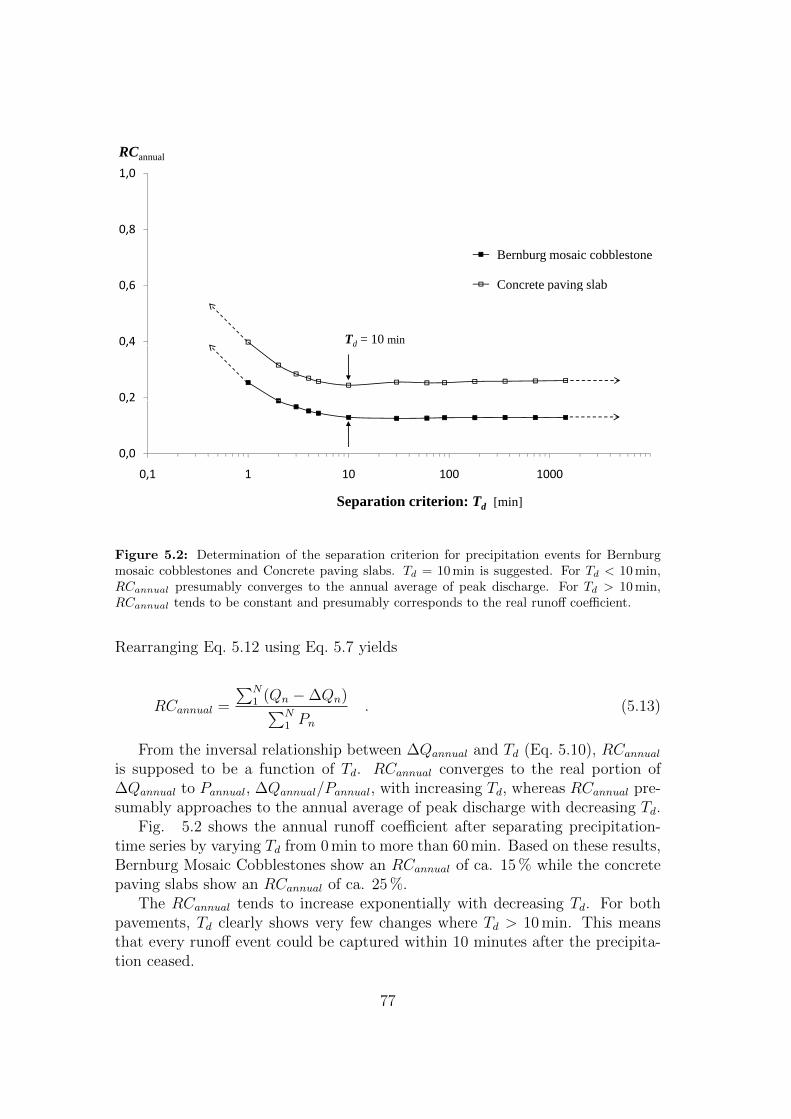
1,0

RCannual

0,8

0,6

Bernburg mosaic cobblestone

Concrete paving slab

0,4

, p g

Td = 10 min

0,2

, d

0 0

0,2

0,0

0,1 1 10 100 1000

Separation criterion: Td [min]

Figure 5.2: Determination of the separation criterion for precipitation events for Bernburgmosaic cobblestones and Concrete paving slabs. Td = 10 min is suggested. For Td < 10 min,RCannual presumably converges to the annual average of peak discharge. For Td > 10 min,RCannual tends to be constant and presumably corresponds to the real runoff coefficient.

Rearranging Eq. 5.12 using Eq. 5.7 yields

RCannual =

∑N1 (Qn −∆Qn)∑N

1 Pn

. (5.13)

From the inversal relationship between ∆Qannual and Td (Eq. 5.10), RCannual

is supposed to be a function of Td. RCannual converges to the real portion of∆Qannual to Pannual, ∆Qannual/Pannual, with increasing Td, whereas RCannual pre-sumably approaches to the annual average of peak discharge with decreasing Td.

Fig. 5.2 shows the annual runoff coefficient after separating precipitation-time series by varying Td from 0 min to more than 60 min. Based on these results,Bernburg Mosaic Cobblestones show an RCannual of ca. 15 % while the concretepaving slabs show an RCannual of ca. 25 %.

The RCannual tends to increase exponentially with decreasing Td. For bothpavements, Td clearly shows very few changes where Td > 10 min. This meansthat every runoff event could be captured within 10 minutes after the precipita-tion ceased.

77

5.1.3 Cumulative Precipitation Frequency Functions

For the dynamics of the water balance, the precipitation event frequency mayplay a large role (Wessolek and Facklam, 1997; Ferguson, 2005; Flotter, 2006).However, the observations of the events were based on less precise temporal reso-lution. The daily precipitation sum has previously been used to explain the roleof event frequency for water balance dynamics. In my study, the separation ofevents from the paved weighable lysimeter enables a more precise definition ofthe event parameter.

For the annual water balance, one can describe the set of all rainfall eventsas a sequence of the random phenomena, caused by uncountable, unpredictable,and complex impact factors in climatic time space. In the Eq. 5.8 (see Chap. 5.1)this random sequence is defined as the population (P) of single rainfall eventsPn, which includes parameters like depth (Pn), intensity (rn), and duration (Tn).Hereby, n denotes the index number of events, and its maximum may be identicalto the annual event number N , which is strongly specified by Td of the monitoringsystem.

If the subpart of P, in which the events have the same intensity r, is describedas the subset

P [r] = {Pn | rn = r, n ∈ [1, N(r)] } , (5.14)

the total precipitation sum of population P[r] can be defined as following:

P (r) =

N(r)∑1

Pn , (5.15)

where N(r) = the size of P[r] and the number of events that have the sameintensity r.

From these formulations, the cumulative precipitation PF (r) as well as thecumulative event number NF (r) are defined as the following:

PF (r) =

∫ r

0

P (r) dr , (5.16)

and

NF (r) =

∫ r

0

N(r) dr . (5.17)

The cumulative precipitation frequency functions give the total sum as wellas the total number of events that belong to an arranged class by the eventparameters. In Eq. 5.16, rainfall event intensity is chosen as event parameter.

78

0 4

0,6

0,8

1p(t): precipitation

q(t): runoff

r: event intensity

Pn

Pn-2

Pn+1

Pn-3

08.10.2009

ipita

tion

[mm

]

1

0

0,2

0,4

00:59

01:40

02:00

02:19

02:28

04:56

05:12

07:18

07:46

09:15

10:35

12:14

Pn-4

Pn-5

Prec

i

time

Pn-1

Figure 5.3: An example of precipitation events from Oct. 8th 2009. The precipitation eventsthat are separated from each other have different runoff impacts. A good paved lysimetersystem should minimize the ∆Q and Td.

79

When r is set on the maximum of event intensities measured during a year, rm,PF (r) may yield the annual precipitation sum. Similarly, NF (r) indicates thetotal event number in period and NF (r) equals the total event number of theyear, when r = rm.

By means of PF (r) and NF (r) functions, the intensity range of the typicalevents for a region can be figured out. For the Berlin region, the r = 0.05 and0.1 mm/min are considered pertinent intensity values for interpreting the annualrainfall distribution (Fig. 5.4).

5.2 Annual Precipitation-Event Frequency

The annual precipitation-event frequency is obtained based on the rainfall databetween May 2009 and April 2010, using Td = 10 min. On the right vertical axes,Fig. 5.4 shows the curve progress of PF (r) as well as of NF (r). The left verticalaxes show the percentages of cumulative sum and number, PF (r)/PF (rm) andNF (r)/NF (rm), respectively. During the measurement period of 2009/10, 932precipitation events were acquired, the total precipitation sum was on 537 mm,and the maximum event intensity, rm, is ca. 0.45 mm/min.

The smallest events (r < 0.01 mm/min) can presumably barely produce runoffand also not massive enough to infiltrate against the wetting capacity of surface.In addition, these small amounts of precipitation likely evaporate immediatelyafter the end of the event. This is particularly true for the urban pavements dueto their usual high temperature and dryness. For events with r < 0.01 mm/min,although the event frequency was over 60 %, its cumulative precipitation sum wasunder 10 % of annual precipitation sum.

The strong events presumably have high runoff coefficients, and the infiltra-tion capacity of soil surface can be quickly used up. For flood protection, therunoff coefficient was considered as independent of rainfall intensity and nor-mally assessed as a high value (DWA-A, 2005). The NF (r) has a slow inclineafter r > 0.1 mm/min and PF (r) is about 25 % between 0.1 < r < rm. Thehigher the rainfall event intensity becomes, the more slowly the PF (r) inclines.This means that the normal events play the more considerable role than the stormevents for the annual water balance.

The normal events (those with intensities between 0.01 < r < 0.1 mm/min)may variously impact runoff and infiltration processes. These dynamics may bedetermined by the rainfall intensity and duration. Because the average eventscomprise more than 60 % of annual precipitation and more than 40 % of frequencyfor the measurement period 2009/10, it is important to clarify the role of normalevents in the water balance dynamics.

In Tab. 5.2, the monthly cumulative precipitation frequencies are listed us-ing the threshold values of rainfall-event intensity: 0.01, 0.05, and 0.1 mm/min.Flotter (2006) attempted to regulate some event-based specific intensities. His

80

50090

100

40070

80

30060

70

mm

]

F(r

m)[

%]

20040

50

PF(r

)[

PF(r

)/PF

10020

30

PF

0

100

0

10

00

0 0,05 0,1 0,15 0,2 0,25 0,3 0,35 0,4 0,45

r [mm/min]

0,01

(a) Cumulative precipitation sum.

900

90

100

700

800

70

80

500

60060

70)(r

m)[

%]

400

500

40

50

NF

(r)

F(r

)/N

F(

200

300

20

30

NF

10010

20

00

0 0,05 0,1 0,15 0,2 0,25 0,3 0,35 0,4 0,45

r [mm/min]

0,01

(b) Cumulative precipitation number.

Figure 5.4: The cumulative precipitation depth PF (r) and the cumulative event numberNF (r). All are also presented in percent value. The cumulative precipitation sum and numberof small events take big percentage of annual frequency.

81

work used one hour as the reference interval to define a rainfall event. After him,small events have r < 0.5 mm/h (corresponding to 0.008 mm/min), normal events0.5 < r < 4.0 mm/h (0.07 mm/min), and storm events have r > 0.07 mm/min forHamburg region, Germany. These almost agree with the thresholds of Tab. 5.2for the Berlin region. The normal events are supposed to make up the majorpercentage of annual rainfall.

For summer periods, the PF (0.1) (the cumulative precipitation sum of eventswith the r < 0.1) varies widely. While PF (0.1) is less than ca. 40 % for July andAugust of 2009, it is about between 70 % and 100 % for the other months. Further,all events had intensity of almost r < 0.1 between November 2009 and Feburary2010, which implies a high frequency of small events during winter time. Thewater balance process is supposed to progress in a different fashion depending onthe precipitation-event frequency. Hence, it is of interest to compare the rainfall-runoffrelathionship of, e.g., July and August of 2009 with that of November 2009(see Chap. 5.3.2).

5.3 Water Balance 2009–2010

5.3.1 Groundwater Recharge and Evaporation

Using the paved weighable lysimeters, the water budget parameters between May2009 and April 2010 were measured. The Hellmann rain gauge delivered theannual precipitation of Pannual = 537 mm.

The annual water balance WB was accumulated by the single measurementvalues of runoff (RO), seepage (GW ), changeable water storage (∆W ), and evap-oration (ET ), analogous to the Eq. 3.1

Although the water balance (WB) is supposed to near to the Pannual, that fromthe lysimeter with Bernburg mosaic cobblestone (abbreviated as MCS throughbelow), WBMCS, was ca. 457 mm and that of concrete paving slab (abbreviatedas CPS throughout below) ca. 452 mm, respectively (Fig. 5.5). The lysimeterwith resolution of 0.1 mm was apparently not precise enough to capture the small-est events of r < 0.01 mm/min, which the Hellmann gauge was able to measure.Therefore, PF (0.01) = 59.5 from the Tab. 5.2 can potentially explain the gapbetween water balances and precipitation for MCS and CPS (80 mm and 75 mm,respectively).

Furthermore, the measurement of snow precipitation during the winter periodmight have had several failures at very cold and windy conditions because theunheated Hellmann gauge is not able to deliver the accurate snow value. Inaddition, the frozen lysimeter also cannot react precisely against the long, steadyblowing-away of snow layer. Thus, this may be reason for very low precipitationsum of January 2010 (Tab. 5.1).

The annual groundwater recharges for MCS and CPS were ca. 383.3 mm (ca.

82

600

500

400

th [m

m]

Precipitation

300

ater

dep

t RO (MCS)

GW (MCS)

200wa

ET (MCS)

water balance (MCS)100

( )

0

2009.05

2009.06

2009.07

2009.08

2009.09

2009.10

2009.11

2009.12

2010.01

2010.02

2010.03

2010.04

(a) Bernburg mosaic cobblestone.

600

500

400

th [m

m]

Precipitation

300

ater

dep

t RO (CPS)

GW (CPS)

200wa

ET (CPS)

water balance (CPS)100

0

2009.05

2009.06

2009.07

2009.08

2009.09

2009.10

2009.11

2009.12

2010.01

2010.02

2010.03

2010.04

(b) Concrete paving slab.

Figure 5.5: Annual water balance 2009/10.

83

71.4 % of Pannual) and ca. 348.2 mm (64.9 % of Pannual), respectively, values thatcan be classified as surprisingly high.

Wessolek (1993), Senatsverwaltung Berlin fur Stadtentwicklung (2001), andFlotter (2006) already specified very high rates of groundwater recharge despitethe high degrees of sealing. They concluded that the reason might lie in the highfrequency of days with small events. The rainwater of small events could remainwithin the wetting capacity space without flowing away, and then could infiltrateor evaporate immediately after the end of the event. Hence, the reasonableselection of seam materials and pavement type can positively affect the annualwater balance by enhancing the surface storage.

Both surfaces showed higher groundwater recharge in the winter period thanin the summer period. The seepage water continuously flowed from groundwatersystem of both lysimeters. MCS has had slightly higher incline of the ground-water recharge rate than CPS. In sum, there was not a big difference betweengroundwater recharge beneath both surfaces.

The annual evaporation rates are ca. 83.4 mm (ca. 15.5 % of Pannual) fromMCS and ca. 55.0 mm (ca. 10.2 % of Pannual) from CPS. The periodic evapo-ration of MCS was always higher than that of CPS. Despite the big differencein the seam portion between MCS (40 %)and CPS (7 %), the difference in theirevaporation rates was rarely large. In the winter period they showed almost sim-ilar evaporation, while in summer periods the evaporation of MCS was visiblybigger than that of CPS.

Fig. 5.6 illustrates an example of evaporation from MCS and CPS betweenJuly 20th to 25th 2009, accompanied by grass reference evapotranspiration fromFAO lysimeter. The seven rainfall events shown are detected. For every events, alllysimeter surface indicated a rapid increase in evaporation directly after the event.During the warmer daytime temperatures, the evapotranspiration performanceof the grass surface is significantly greater than that of the paved surfaces. Theactual evaporation from the paved surfaces depends on the surface water supplyand climate conditions at the time of day.

During the daytime of July 21st, the evaporation from MCS is much greaterthan from CPS. It was induced from the storm event late on July 20th. Theevent was sufficiently intense to store a certain amount of surface water withinthe surface storage. After the rainfall ceased, the surface water supply of CPSwas exhausted through the night, while the surface water of MCS was still notexhausted.

In contrast to that, both paved surfaces showed only a small increase in theafternoon of July 23rd and 24, because the surface water supply had been alreadyexhausted. The rainfall event at 05:00 am on July 22nd was not big enough tostore sufficient water in the upper paved soil zone. Additionally, for summerrelation, the drying duration after this event (between 22nd and 24th) was toolong to save surface water for considerable evaporation during the day time ofJuly 23rd.

84

0

58

9

10 0

5

10

6

7

8

9

10

mm

/hou

r]

n [m

m]

Precipitation

ET (grass)

0

5

10

15

4

5

6

7

8

9

10

tatio

n [m

m/h

our]

poratio

n [m

m]

Precipitation

ET (grass)

ET (CPS)

ET (MCS)

0

5

10

15

20

252

3

4

5

6

7

8

9

10

Precipita

tion 

[mm

/hou

r]

Evaporation 

[mm

]

Precipitation

ET (grass)

ET (CPS)

ET (MCS)

midnight

0

5

10

15

20

25

300

1

2

3

4

5

6

7

8

9

10

Precipita

tion 

[mm

/hou

r]

Evaporation 

[mm

]

Precipitation

ET (grass)

ET (CPS)

ET (MCS)

midnight

noon

0

5

10

15

20

25

300

1

2

3

4

5

6

7

8

9

10

Precipita

tion 

[mm

/hou

r]

Evaporation 

[mm

]

Precipitation

ET (grass)

ET (CPS)

ET (MCS)

midnight

noon

0

5

10

15

20

25

300

1

2

3

4

5

6

7

8

9

10

Precipita

tion 

[mm

/hou

r]

Evaporation 

[mm

]

Precipitation

ET (grass)

ET (CPS)

ET (MCS)

midnight

noon

Figure 5.6: Paved surfaces induced a big deficit of evaporation in comparison with the grassreference surface (FAO lysimeter). After various rainfall events, the evaporation behavior ofpavements strongly depends on the surface water, supplied from the event. Occasionally, thepavements with small seam portion also can show a slightly high evaporation, because moresurface water is available immediately from the wetting capacity for short period. However,there is not a significant difference in the evaporation performance between of MCS and CPSpavements for the annual evaporation.

85

Table 5.1: Monthly water balance components and runoff coefficients. P = precipitation in[mm], RO = runoff in [mm], RC = runoff coefficient in [%], GW = groundwater recharge in[mm], ET = evapotranspiration in [mm], and ∆W = in [mm]. (MCS for Bernburg mosaiccobblestones and CPS for Concrete paving slab.)

MCS CPS MCS CPS MCS CPS MCS CPS MCS CPS

2009.05 83.40 11.84 17.13 14.20 20.54 33.04 34.72 15.68 6.62 13.57 15.18

2009.06 85.30 15.96 23.28 18.71 27.29 59.10 59.28 9.08 7.58 -18.00 -20.05

2009.07 48.40 6.50 11.00 13.43 22.73 9.71 12.27 8.91 6.88 5.50 4.10

2009.08 22.80 3.18 5.20 13.93 22.81 20.09 16.16 6.74 4.85 -14.93 -11.08

2009.09 33.00 7.30 10.79 22.11 32.69 26.40 14.04 5.93 3.95 -9.14 0.96

2009.10 86.10 21.85 38.38 25.38 44.57 32.50 26.84 8.30 2.64 16.79 12.17

2009.11 54.40 7.30 15.20 13.42 27.94 44.09 40.79 2.17 1.38 -8.00 -12.14

2009.12 57.00 9.70 15.80 17.02 27.72 32.83 22.87 1.14 1.94 2.14 4.46

2010.01 2.80 0.20 0.30 7.14 10.71 42.02 50.19 6.10 3.79 -26.57 -26.25

2010.02 22.70 0.00 0.70 0.00 3.08 24.22 25.86 9.97 7.95 -25.93 -27.59

2010.03 21.20 0.20 2.20 0.94 10.38 29.57 23.69 3.75 3.44 -14.71 -17.35

2011.04 19.90 0.90 4.60 4.52 23.12 29.66 21.61 5.63 4.01 -16.93 -17.47

total 537.00 84.93 144.57 15.82 26.92 383.27 348.34 83.40 55.03 -96.21 -95.07

GW [mm] ET [mm] ∆W [mm]RO [mm] RC [%]month P [mm]

Interestingly, for event-based observation of evaporation, CPS could tem-porarily have bigger evaporation than MCS, e.g. immediately after the rainfallevents. As shown in Fig. 5.6 was there higher actual evaporation from CPS inthe morning of July 22nd, during the night time of July 21st., and for the timespan after rainfall events on July 25th.

5.3.2 Influence of Rainfall-Runoff Relationshipon Water Balance

The total runoff sums were ca. 84.9 mm (annual runoff rate: 15.8 %) from MCSand ca. 144.6 mm (annual runoff coefficient: 26.9 %) from CPS, out of the totalprecipitation of 537 mm. For months with high precipitation, the monthly runoffsum was also normally high. The annual runoff sum is not as big as the differencein seam portion. Nevertheless, the periodic runoff coefficients of CPS were alwaysbigger than that of MCS (see Fig. 5.5, Tab. 5.1, and Tab. 5.4).

Tab. 5.2 gives an overview of the monthly precipitation frequency classified bythe threshold values of rainfall event intensity. From this table, the cumulativeprecipitation sum (PF (r)) and the cumulative number of events (NF (r)) are cal-culated, the maximum event intensity was also added in order to give informationabout the eventual extreme storm event.

The monthly RC is clearly varying for each pavement through the year. Con-sidering the rainfall event intensity as an impact factor on RC, one can explain

86

Table 5.2: Monthly precipitation-event frequency. The precipitation-event frequency variesfor hydrologic periods. The monthly rainfall event frequency can clarify the water balancedynamics for the annual processes. Events with intensity 0.01 mm/min < r < 0.1 mm/mindominate within the annual precipitation frequency. NF = cumulative event number by givenintensity and PF = cumulative precipitation sum by given intensity, % column beside PF isthe value of PF/PF (rm) and gives the monthly percentage of cumulative precipitation sum tothe monthly precipitation.

r [mm/min]

r m NF PF % NF PF % NF PF % NF PF

≤ r m≤ 0.1≤ 0.01 ≤ 0.05

2009.05 0.23 28 2.8 3.36 60 37.5 44.96 68 59 70.74 74 83.4

2009.06 0.38 44 4.4 5.16 66 26.8 31.42 77 58.6 68.70 80 85.3

2009.07 0.41 28 2.8 5.79 42 11.5 23.76 48 20.2 41.74 62 48.4

2009 08 0 17 16 1 6 7 02 25 4 5 19 74 28 7 1 31 14 33 22 82009.08 0.17 16 1.6 7.02 25 4.5 19.74 28 7.1 31.14 33 22.8

2009.09 0.3 19 1.9 5.76 26 12.4 37.58 34 25.9 78.48 37 33

2009. 10 0.36 102 10.2 11.85 142 46.7 54.24 148 64.4 74.80 153 86.1

2009.11 0.1 97 9.7 17.83 126 48.4 88.97 129 54.4 100.00 129 54.4

2009.12 0.2 117 11.7 20.53 143 55.2 96.84 147 56 98.25 152 57

2010.01 0.05 14 1.4 50.00 16 2.8 100.00 16 2.8 100.00 16 2.8

2010.02 0.05 74 7.4 32.60 99 22.7 100.00 99 22.7 100.00 99 22.7

2010.03 0.1 43 4.3 20.28 59 19.6 92.45 62 21.2 100.00 62 21.2

2010.04 0.2 16 1.6 8.04 28 8.9 44.72 30 10 50.25 35 19.9

annual value 595 59.5 11.08 832 297 55.31 886 402.3 74.92 932 537

this dynamic behavior of the RC. May and June of 2009 had a similar precipi-tation frequency and about the same precipitation sum (83.4 mm and 85.3 mm,respectively). The values of PF (0.1) are nearly the same for both month periods(ca. 59 mm and 70 %). However, the values of PF (0.05) are quite different andthis could be the reason for the smaller RC for May than for June, for bothpavements.

Interestingly, the RC of July and August, 2009 remained almost unchangedfor MCS and CPS, ca. 13.5 % and ca. 23 %, respectively, although the precipi-tation sums in July (48.4 mm) was more than double that in August (22.8 mm).During these two months, PF (0.1)/PF (rm) were smaller than 50 %. Based onthe assumption that the RC tends to remain constant for the storm events withhigh event intensity, the small and normal precipitation events of PF (0.1) couldnot be the primary reason for the difference in the RC. However, the RC of Julyand August 2009 are supposed to have much higher values than other months,which did not happen because the storm events of PF (rm > r > 0.1) wereeither of short duration or of relatively lower intensity. This means that not onlythe intensity (r) but also the event duration (T ) helps the high runoff coefficient.For example, the event of 10.07.2009 15:29:07 lasted only T = 11 minutes, withthe maximum intensity rm = 0.41 mm/min and that of 21.08.2009 19:13:44 onlylasted with T = ca. 70 min, rm = 0.17 mm/min .

87

Table 5.3: The distribution of runoff-producing and non-runoff-producing rainfall events inthe period of 2009/10. A large proportion of rainfall events without runoff can lead to differentdynamics of the annual water balance. This behavior varies according to the kind of pavement.For the mosaic cobble stone, the total number and the sum of events that could produce runoffwas significantly less than for the concrete paving slab.

annual value RCn = 0 RCn ≠ 0 RCn = 0 RCn ≠ 0

N 932 (337*) 274 63 169 168

P [mm] 537 (477.5*) 259.3 218.2 96.2 381.3* the annual value of r > 0.01 mm/min

MCS CPS

In contrast, the RC of September and October 2009 are higher than that ofthe other months, despite of high value of PF (0.1) over ca. 75 %. The reasonis that there were several storm events of long duration with an intensity over0.1 mm/min (e.g. on Oct. 8th, 2009, see Fig. 5.3).

The behavior of RC during November and December, 2009 were also verysimilar, presumably because the precipitation frequencies were almost adequate.

Throughout the winter months, runoff behavior might be completely differentfrom that of summer periods, because surface flow then is provided by not fallingwater, but by melting water. Since melting water may not have any fallingintensity, the infiltration rates are very high and the runoff rate is low.

As analyzed above, the periodical rainfall-runoff relationship strongly dependson the precipitation-event frequency. The rainfall-runoff relationship character-ized by RC is again strongly dependent on event intensity.

During the nth rainfall event, the rainwater is divided into runoff water andinfiltration water at the soil surface as the following:

Pn = ROn + In , (5.18)

and the runoff coeffcient of the event is

RCn =ROn

pn. (5.19)

Depending on the surface properties, the infiltration In provides the primarysource of evaporation and groundwater recharge. If RCn = 0 and, thus, Pn = In,the rainfall event is denoted as a rainfall event without runoff. Tab. 5.3 liststhe total sum and number of rainfall events with (RCn 6= 0) and without runoff(RCn = 0) for both MCS and CPS pavements.

For the annual water balance, the greater the sum of rainfall events withoutrunoff becomes, the more rapidly the RCannual declines. As RCannual declines,

88

Table 5.4: The average runoff coefficients of event ranges according to the intensity.

annual value RCn = 0 RCn ≠ 0 RCn = 0 RCn ≠ 0

N 932 (337*) 274 63 169 168

P [mm] 537 (477.5*) 259.3 218.2 96.2 381.3* the annual value of r > 0.01 mm/min

MCS CPS

more water supply is available for other water balance processes such as ground-water recharge, water storage, and evaporation. As for the precipitation sum ofevents without runoff in 2009/10, the MCS shows a significantly greater valuethan the CPS.

Fig. 5.7 classifies the rainfall event into runoff-producing and non-runoff-producing events by applying border lines. Precipitation-event sum versus eventduration can indirectly state about the rainfall event intensity through the tan-gent of point (P/T ). However, a distinctive selection of such a border line hasan uncertainty. The stronger the event intensity is, the better the possibility ofit being runoff-producing. For CPS, selecting such an intensity is much clearerthan for MCS. Still, some events exist that are runoff-producing but are underdashed line, and that are non-runoff-producing but over the dashed line.

With some exceptions, it is clear that a certain amount of rainfall is neededin order to be effective for runoff. This means, in other words, that pavementshave a certain surface space (surface storage, Vs) in which the rain water can bedefinitely stored without running off. Presumably, the surface storage of MCS isbigger than that of CPS, because MCS simply has more volume space throughthe higher seam portion and rougher surface.

Fig. 5.8 illustrates the event runoff coefficient acquired in 2009/10. A slightincrease of RC with increasing event intensity r is shown for both pavements. Onone hand, the fluctuation of the relationship still exists, presumably because thediagram does not consider the surface storage Vs. On the other hand, there arealso some events with high rainfall intensity that do not produce runoff, whichpresumably is due to the insufficient rainfall sum.

Tab. 5.4 shows the average runoff coefficients, where rainfall events are classi-fied into the range intensity. It is clear that CPS generally has a higher RC thanMCS. In sum, for the investigation of rainfall-runoff relationship, both surfacestorage and rainfall event intensity play meaningful roles.

89

18

14

16

10

12

]

8

10

P [m

m]

non-runoff-producing

runoff-producing

4

6

0

2

0 50 100 150 200 250 300

T [min]

(a) Bernburg mosaic cobblestone.

18

14

16

10

12

m]

8

10

P [

mm

non-runoff-producing

runoff-producing

4

6

0

2

0 50 100 150 200 250 300

T [min]

(b) Concrete paving slab.

Figure 5.7: Runoff-producing and non-producing precipitation-events: The rainfall eventswith lower intensity than runoff-producing intensity are not effective to produce runoff. Theevents with smaller rainfall sum than a surface storage are also not effective to produce runoff.MCS (Berburg mosaic cobblestone) shows greater runoff-producing intensity and bigger surfacestorage than CPS (Concrete paving slab).

90

0,4

0,6

0,8

1R

C

y = 0,1197ln(x) + 0,519R² = 0,4575

0

0,2

0,4

0,6

0,8

1

0 0,1 0,2 0,3 0,4 0,5

RC

r [mm/min]

(a) Bernburg mosaic cobblestone

y = 0,083ln(x) + 0,5374R² = 0,2285

0,4

0,6

0,8

1

RC

y = 0,083ln(x) + 0,5374R² = 0,2285

0

0,2

0,4

0,6

0,8

1

0 0,1 0,2 0,3 0,4 0,5

RC

r [mm/min]

(b) Concrete paving slab

Figure 5.8: Runoff coefficients versus rainfall event intensity.

91

Chapter 6

Model Concept for RunoffDynamicsof Paved Soil Surface

The most regional runoff models need more appropriate approaches for assessingthe impact of urban development on actual runoff behavior, because they do notinclude variables that typically are used to reflect changes in urban watershedconditions. One of the most widely used basic approaches is the rational conceptwhich was first suggested in 1889 by Kuichiling (McCuen, 2004) and is primarilyused for design problems for small urban areas, such as the dimensioning of in-lets and culverts. But it is known that the approach of rational methods is notsufficiently adequate for design problems where watershed storage is significant,such as in permeably paved soils. Hence, in the last decades, lots of studies aboutinfiltration properties of soils and porous materials have been done (Green andAmpt, 1912; Philip, 1957a,b; Bear, 1972; Hillel, 1998). For watersheds that arenon-homogeneous and undergoing to land use change, especially under urbaniza-tion, watershed design work is usually based on hydrograph concept, which doesnot inherently exclude the involved processes. It is essential to study the runoffdynamics of the paved soil surface for urban hydrograph research.

In this chapter, two models for runoff calculation are suggested: the surfacestorage model for runoff concentration processes and the intensity-dependentrunoff coefficient model for runoff processes, which include both precipitation-event parameters and surface hydrologic parameters. From the profound obser-vation of the rainfall event processes, the runoff concentration process and therunoff process are described in detailed subprocesses.

92

6.1 Surface Water Process

6.1.1 Phase of Runoff and Infiltration Process

The overall rainfall-runoff relationship during a certain period varies by surfacehydrologic parameters of the pavement, e.g. surface storage and infiltration per-formance, while the runoff dynamics during a certain precipitation event can beclarified by describing rainfall event parameters such as event intensity and eventduration.

For comprehending the event-dependent runoff dynamics on small plots, asimplemented in our lysimeter system, the rainfall event process can be considereddifferently than the water-pond hydrologic process.

(i) For the water-pond hydrologic process, the infiltration is only related tothe soil-physical properties, controlled by the water head pressure. It does notrequire any intensity factors. Thus, experiments under water-ponded conditionsserve to clarify the soil physical behaviors. Here, it is presumed that the sufficientwater supply is provided to demonstrate the potential infiltration capacity.

(ii) For the precipitation event process, the water supply for infiltration doesnot always sufficiently exist. The high potential infiltration capacity cannot bedemonstrated fully. Thus, the precipitation event produces runoff with differenteffectiveness. For the precipitation events without runoff (non-runoff-producingevents), the water is completely taken up in the form of infiltration, evaporationand interception at the paved soil surface.

Depending on the surface storage volume, the runoff-producing event goesthrough two stages: the runoff concentration process and the runoff process,which can be again separated into two detailed processes (see Fig. 6.1).

During the runoff concentration process, the precipitation sum (called ini-tial loss, denoted as Pa) is affected not only by the infiltration, but also bythe interception, the depression storage, the short-term evaporation, and otherintensity-kinetic effects.

Interception is a complex interaction of retention and detention processesabove the soil surface. This process is a part of initial loss because it occursat the beginning of a rainfall event and this lost water cannot take part in thegroundwater and vegetation water processes. Infiltration describes the seepage offluid through pore and cavity into the lithosphere (DIN 4049-1, 1989). Water caninfiltrate into the soil when the hydraulic potential at the surface is bigger thanin the deeper soil zone. Considering interception also as a part of infiltration atthe beginning of a rain event, the total infiltration will always have a high rateat the beginning.

In addition, the evaporation is also supposed to play a big role at the beginningof the event. In general, the surface of paved soil has high temperature anda high heat capacity dominates in paving materials, particularly under urbanconditions. Once it rains and the paved soil has again enough water supply to

93

cool the microclimate at the surface, the high heat energy will be released.Fig. 6.1 shows a rainfall event with a small antecedent event (from the mea-

surement of July 23rd, 2009). As for the antecedent sub-event with the intensityof max. 0.4 mm/5 min, the small first runoff-flush is generated earlier from theconcrete paving slab (CPS) than from the Bernburg mosaic cobblestone (MSC).Due to the bigger surface storage of MCS, no considerable runoff was inducedfrom MCS for the first ca. 30 minutes. When the main rainfall event starts, therunoff peak discharge of CPS is much higher than that of MCS.

The graphs clearly show the higher infiltration performance and the lowerrunoff from MCS than from CPS. For both surfaces the initial infiltration rateshave high values, which decline rapidly to a fairly constant rate (final infiltrationrate).

For CPS, the final infiltration rate appears to be settling after ca. 70 minutes,with the runoff not stopping. However, the runoff from MCS lasts for ca. 50minutes much shorter than the runoff from CPS. This is a result of the low initialinfiltration capacity of CPS. Essentially all the rain water of MCS infiltrates afterthe final infiltration rate is reached. After more than four hours of rain, runoffof CPS takes place visibly once again and the infiltration rate tends to remainconstant, while MCS has very little runoff and nearly all rain water infiltrates.

It is notable that the observation shows that the infiltration curves, i(t), donot correlate with the precipitation curves, p(t), during final infiltration. Theeventual fluctuation of i(t) of final infiltration is caused by the inaccuracy ofthe temporal measurement. The runoff curves, q(t), clearly change with theprecipitation curves, which means these represent the remaining precipitationwater after removing the constant final infiltration.

The rainfall-runoff process can be described in 3 consecutive processes affect-ing the soil infiltration capacity:

(i) the runoff concentration process: as long as the precipitation event is notintense enough, no runoff water occurs. The precipitation up to this point iscompletely taken up as initial loss;

(ii) the initial infiltration process: after the rainfall intensity exceeds the infil-tration capacity, the runoff process takes place. The infiltration rate declines withtime elapsing while the soil surface is under the unsaturated state. The uppersoil zone still has a high infiltration capacity. The infiltration curve is stronglyinfluenced by the precipitation intensity;

(iii) the final infiltration process: the infiltration rate converges to the con-stant value of the final infiltration rate and the soil surface reaches the steadyinfiltration under saturated state. The final infiltration rate may theoreticallycorrespond to the value of the constant hydraulic conductivity of the paved soil.When the precipitation during this process is not intense enough, the rainwaterwill infiltrate completely without reaching the saturated soil state and no waterwill run off.

94

2,5

p, q, i [mm/5min]

Pa Pu

2

1,51,5p: precipitation

i: infiltration (MCS)

q: r noff (MCS)1 q: runoff (MCS)

0,5

0

2:35

2:45

2:55

3:05

3:15

3:25

3:35

3:45

3:55

4:05

4:15

4:25

4:35

4:45

4:55

5:05

5:15

5:25

5:35

5:45

5:55

6:05

6:15

6:25

6:30

(a) Bernburg mosaic cobblestone (MCS)

2,5

p, q, i [mm/5min]

Pa Pu Ps

2

1,51,5p: precipitation

i: infiltration (CPS)

ff (CPS)1 q: runoff (CPS)

0,5

0

2:35

2:45

2:55

3:05

3:15

3:25

3:35

3:45

3:55

4:05

4:15

4:25

4:35

4:45

4:55

5:05

5:15

5:25

5:35

5:45

5:55

6:05

6:15

6:25

6:30

(b) Concrete paving slab (CPS)

Figure 6.1: A precipitation event from Juli 23rd, 2009. The surface water process can beobserved in 3 phases: the runoff concentration, the initial infiltration and the final infiltra-tion. The surface water process during these 3 phases has a different relationship with theprecipitation due to the changing infiltration behavior of the soil surface.

95

6.1.2 Runoff Coefficient

The runoff coefficient, RC, is the proportion of the total produced runoff tothe total precipitation. This can relate a whole precipitation period, as it isformulated for the annual water balance in Eq. 5.12, or a single event, as inEq. 5.19. RC is a dynamic function of rainfall intensity and the surface hydrologicparameters.

The rainfall event sum can be described from Fig. 6.1 as follows:

P = Pa + Pu + Ps , (6.1)

where Pa = initial loss, Pu = precipitation sum during initial infiltration(t < ts), and Ps = precipitation sum during final infiltration (t ≥ ts), where tsis the start time of final infiltration. Here, the sum of Pu and Ps makes up theeffective precipitation sum (Pe) that directly causes the runoff:

Pe = P − Pa = Pu + Ps . (6.2)

The sums of sub-precipitation Pa, Pu, and Ps are normally calculated as in-tegrals of rainfall rate as follows:

Pa =

∫ tc

to

p dt ,

Pu =

∫ ts

tc

p dt ,

Ps =

∫ tp

ts

p dt .

(6.3)

Let us define the proportion of the runoff to the effective precipitation sum asthe effective runoff coefficient, RCe:

RCe =RO

Pe

. (6.4)

Rearranging Eq. 5.19 with Eq. 6.4, RC will be restated as follows:

RC =Pe

P· RCe = (1 − Pa

P) · RCe . (6.5)

Eq. 6.5 clarifies that the runoff coefficient can be considered a function of bothinitial loss during runoff concentration and the effective runoff coefficient duringthe direct runoff process.

96

During the runoff process, the runoff behavior shows a different intensity-dependency before and after the the saturated time point ts. The runoff sum canbe described in detail with the initial runoff ROu during tc < t < ts and the finalrunoff ROs during t ≥ ts:

RO = ROu +ROs , (6.6)

where the components of runoff are calculated as follows:

ROu =

∫ ts

tc

qdt ,

ROs =

∫ tp

ts

qdt .

(6.7)

Let us define the initial runoff coefficient and final runoff coefficient, respec-tively, as the following:

RCu =ROu

Pu

,

RCs =ROs

Ps

.

(6.8)

From Eq. 6.2 and Eq. 6.4, the runoff coefficient during the direct runoff processis

RCe =RO

Pe

=Pu ·RCu + Ps ·RCs

Pu + Ps

. (6.9)

Finally, from Eq. 6.5, the runoff coefficient of the total precipitation event isdefined as the following:

RC = (1− Pa

P) · Pu ·RCu + Ps ·RCs

Pu + Ps

. (6.10)

It is assumed that the RCu is strongly dependent on the precipitation eventintensity and that no relationship between RCs and rainfall intensity (r) exists,because the runoff is only the difference between the precipitation and the finalinfiltration.

When the final infiltration process is not reached during the event and Ps = 0is negligible, as Fig. 6.1 (a) shows, then the runoff coefficient is

RC = (1− Pa

P) ·RCu . (6.11)

Fig. 6.2 compares the P -RO-relationship and the Pe-RO-relationship, wherethe runoff sum more clearly relates to the effective precipitation sum.

97

20

15

[mm

]

10

epth: R

O

y = 0,3949x ‐ 0,1986R² = 0,66935ru

noff de

,

00

0 5 10 15 20

rainfall event depth: P [mm]

1(a)

20

15

[mm

]

0 689 0 2669

10

epth: R

O

y = 0,4689x ‐ 0,2669R² = 0,7043

5runo

ff de

00

0 5 10 15 20

rainfall event depth: P [mm]

1(b)

20   

15

[mm

]

10

epth: R

O

y = 0,5381x + 0,0229R² = 0,8601

5runo

ff de

00

0 5 10 15 20

effective rainfall event depth: Pe [mm]

(c)

20   

15

[mm

]

y = 0,67x ‐ 0,179910

epth: R

O

R² = 0,8579

5runo

ff de

00

0 5 10 15 20

effective rainfall event depth: Pe [mm]

(d)

Figure 6.2: Precipitation-runoff Relationship on the paved surfaces from Bernburg mosaiccobblestone and Concrete paving slab: (a) and (b) show the relationship of P vs. RO for MCSand CPS, respectively, while (c) and (d) show the relationship of Pe vs. RO for MCS and CPS,respectively. The runoff sum, RO is more clearly related to the effective precipitation sum, Pe,than to the precipitation event sum, P .

98

6.2 Surface Storage Model

6.2.1 Runoff Concentration Process

The runoff concentration process is the first phase of the surface water processduring a precipitation event. The infiltration capacity during the concentrationprocess is impacted by the soil moisture and the filling state of the surface storage.The runoff concentration is an intensity-controlled process.

In the conventional regional runoff calculation models, it is assumed that acertain portion of regional retention capacity is responsible for initial loss. Basedon this approach, runoff can arise without completely using the regional retentioncapacity that is equivalent to the surface storage capacity for the small field plots.Initial loss was treated as a constant term for the watershed.

Based on the high temporal resolution of the weighable lysimeter and WTBsystem, the initial loss and runoff concentration duration are obtained preciselyfor the period between May, 2009 and April, 2010. Fig. 6.3 presents the initialloss (Pa) versus the rainfall event sum (P ) for Bernburg mosaic cobblestone andconcrete paving slab.

For runoff-producing events, the average value of Pa from MCS accounts forabout 1.06 liter, while it is about 0.66 liter for CPS, due to the fact that MCShas a higher seam portion (d) and surface depression volume. The reason forthe dissipation of the Pa may lie in the event dependency. The less intense therainfall event is, the more efficiently the surface storage can take the buffer rolefor supplying ponding water.

For non-runoff-producing events, the total precipitation water appears com-pletely in form of initial loss. Both pavements showed a maximum Pa of over5 liters, which is extremely higher than the average initial loss. This has animportant meaning for dynamic surface water process.

For small field plots, like the lysimeter surfaces used in the study, the approachassums that runoff does not occur until the surface storage is used up completely.Predominantly, pavement always has a certain topographical volume (depressionvolume) built from surface morphology and seam geometry, which makes up a bigportion of total surface storage. As the soil of seam materials normally has pores,paving material is also assumed to have a certain volume of pores, especially theconcrete products like CPS. These porous volumes also contribute to surfacestorage volume (Mansell and Rollet, 2009; Starke, 2010). Seam portion is animportant indicator for the surface storage Vs.

For pavements with a small seam portion, Vs causes the retention of rainwaterat the surface and prevents rainwater from flowing immediately into the soil.However, in case of a large seam portion, more rainwater can fall directly onto theseam space without being stored in surface storage. In such a case the infiltrationprocess becomes more dominant than in the case of a small seam portion. Aschematic of surface storage is shown in Fig. 6.4.

99

20

15

mm

]

10

Pa[m

non-runoff-producing

runoff-producing

y = 0,0303x + 1,06935

runoff-producing

R² = 0,032

00

0 5 10 15 20

P [mm]

(a) Bernburg mosaic cobblestone

20

15

mm

]

10

Pa[m

non-runoff-producing

runoff-producing

y = 0,0284x + 0,66025

runoff producing

R² = 0,0304

00

0 5 10 15 20

P [mm]

(b) Concrete paving stone

Figure 6.3: Initial loss (Pa) versus precipitation depth (P ): the initial loss is not related toP . Permeably paved surfaces have a minimum of initial loss, rainfall event is runoff-effectivewhen the rainfall sum is greater than this minimum of initial loss, which may correspond tothe surface storage.

100

In considering surface storage, two kind of processes are of interest.(i) Non-ponding process: the soil surface can never be flooded. Rainfall in-

tensity is low enough that the water uptake process is dominant. Rainfall eventsthat do not produce runoff can be classified as such. The infiltration capacity ofthe soil surface is higher than the precipitation intensity, so the surface storagenever gets filled completely;

(ii) Pre-ponding process: immediately before the runoff generation, surfacestorage is about to be used up. At this stage, the soil surface almost reaches thepond-like state. The rainfall will produce runoff, but has not yet done so;

The non-ponding and pre-ponding process will be skipped when the surfacestorage has not emptied completely since the previous (e.g. big storm) event;e.g., a storm event is preceded by insufficient drying period. The runoff processcan only begin if the rainfall intensity exceeds the infiltration capacity sufficientlyenough to build a pond-like water layer on the surface, which will continuouslyflow down in the form of runoff by gravity along the surface gradient. The amountof runoff is calculated as the remaining amount of the precipitation water that isnot involved in the initial loss and infiltration processes.

During the initial loss process, the water uptake at the paved surface is dividedinto two processes: in the first, one part of the falling rainwater percolates intothe soil (infiltration process) while in the second, the remaining rainwater fills upas surface storage (ponding process).

Pa = Vs + Vr , (6.12)

where Pa = initial loss, Vs = volume of surface storage, and Vr = volume ofinfiltrated water.

In the aspects of intensity, Eq. 6.12 can be restated as below:

r = vs + vr , (6.13)

where r = rainfall intensity, vs = ponding rate, and vr = infiltration rate.The ponding rate vs and infiltration rate vr are strictly controlled by rainfall

intensity r. When r is small enough to sufficiently infiltrate but not high enoughto fill the surface storage, then vr almost equals to r. But, when the rainwaterintensity r becomes big enough to quickly fill the surface storage, then the infil-tration rate nears a constant maximum ro. When r > ro, the ponding rate vsdominates the initial loss process, and runoff is going to be generated after theconcentration duration of Tc. Therefore, let us consider the threshold intensityvalue ro as “runoff-producing intensity”. ro is an important surface hydrologicparameter for modeling the surface storage process.

The infiltration rate vr can be described as a function of r, as illustrated inFig. 6.4:

101

(a) Scheme of Surface Storage (Vs: surface storage volume, d: seam portion).

(b) Relationship between the infiltration rate vr, ponding rate vs, and the rainfallevent intensity r (ro: runoff-producing intensity).

Figure 6.4: Surface storage is characterized by the seam portion and the soil physical prop-erties of the seam soil and paving material, the topography and the geometry of the pavementstructure.

102

Assuming that the volume value of Vs and the function of vr by r

vr = f(r) (6.14)

are known for the paved soil, the runoff concentration duration Tc is calculatedas follows:

Tc =Vsvs

=Vs

r − f(r)(6.15)

From Eq. 6.13 and Eq. 6.15, the volume of infiltration water during initialloss can be described as

Vr = vr · Tc (6.16)

If vs is very small, Tc converges to an unlimited value, and Vr also becomevery big. Therefore, from Eq. 6.12, Pa will increase exponentially.

At the beginning of rainfall, the infiltrability of soil is high. The infiltrabilitydecreases to a certain constant infiltration (final infiltration b) is arrived at bysaturation time ts. . Assuming that the soil surface is completely dried throughevaporation prior to precipitation, the lower the beginning intensity r is, the morewater will be infiltrated in the form of initial loss Pa (see Figure 6.7). Herein, wecan see that the beginning of the rainfall process is critical in determining theponding of surface storage (ponding time and filling state) and infiltration curve.After the saturated soil state is reached, the runoff is only the rest of the steadyinfiltration; therefore we cannot say that the runoff coefficient RC in this phasealso dependent on rainfall intensity.

6.2.2 Surface Storage Model using Hyperbolic Tangent

The runoff concentration process depends both on the infiltration capacity of thesurface and the surface storage. Theoretically, there is not an exact boundarybetween the non-ponding and preponding process. In Fig. 6.4, ro indicates thethreshold rate by which the transition from non-ponding to pre-ponding willoccur during the initial loss. Thus, ro wil be called the “pre-ponding infiltration”rate or the “runoff-producing intensity”.

In order to simulate the slight transition between non-ponding and pre-pondingprocess, the “Tangent Hyperbolic Function (tanh)”´ is applied.

tanh x =ex − e−x

ex + e−x(6.17)

103

vr , vs

roo

vs

ro

vr

0

0

rro

Figure 6.5: The tangent hyperbolic function is suggested for the approximation of the rela-tionship of Eq. 6.14 (compare with Fig. 6.4). Here, vr = infiltration rate , vs = ponding rate ,r = rainfall event intensity, and ro = runoff-producing intensity.

By means of the tanh function, the relationship between the rainfall intensity andinfiltration during runoff concentration can be mathematically described. We canconsider 3 phases of the funciont in Fig. 6.5.

(i) The infiltration rate vr increases together with the rainfall intensity untilit is sufficiently smaller than runoff-producing intensity ro.

(ii) By the range of ro, vr starts nearing to ro.(iii) After the rainfall intensity r is sufficiently bigger than ro, vr remains

permanently constant.The function of Eq. 6.14 is

vr = ro · tanhr

ro, (6.18)

and from Eq. 6.13 and Eq. 6.15, the runoff concentration duration is

104

Tc =Vsvs

=Vs

r − ro · tanhr

ro

. (6.19)

Therefore, the initial loss can be derived as the following using surface storage,runoff-producing intensity, and rainfall intensity:

Pa = r · Tc = Vs · (1−ror· tanh r

ro)−1 . (6.20)

This relationship clarifies that the initial loss results from the interplay be-tween the rainfall parameter and the surface hydrologic parameters. In Fig. 6.6,the minimum initial loss (Pa) is the surface storage (Vs), which means that thesurface storage needs to be completely used up in order to produce runoff. Theinitial loss can grow to an unlimited value when the rainfall intensity is muchsmaller than the runoff-producing intensity, due to the indeterminable runoffconcentration duration (Tc) for r � ro.

Pa

Vs

0

0

rro

Figure 6.6: Surface storage model for the runoff concentration process: the minimum of initialloss (Pa) is the surface storage (Vs), which means that the surface storage needs to be completelyused up in order to produce runoff. The initial loss can grow to an unlimited value when therainfall intensity is much smaller than the runoff-producing intensity due to the indeterminablerunoff concentration duration (Tc) for r � ro.

105

6.3 Runoff Coefficient Model

6.3.1 Description of Rain-pond Infiltration Process

One can determine the infiltration curve when the runoff process can be observedin high temporal resolution. The measurement of runoff is much easier thanthat of infiltration, because the former process takes place in the visible surfacezone, while the latter takes place in time-related (hysteretic) soil moisture in theinvisible soil zone, which is afflicted with measurement difficulty and inaccuracy.

The infiltration rate decreases more or less quickly with the time elapsed,depending on the surface properties (Fig. 6.1). At a certain time, the soil sur-face reaches a saturated state with constant infiltration rate (b). Excepting thepossibility that the escaping air bubbles from the soil can further heighten theinfiltration rate again, the infiltration rate will arrive at a final constant valuethat may relate to the constant hydraulic conductivity of the paved soil. In pastexperiments, many paved surfaces arrived at the final infiltration state more orless within the 60 minutes after rainfall began (Flotter, 2006; Illgen et al., 2007).

In this study, the infiltration approach of Rubin (1966) and Swartzendruberand Hillel (1975) is used for the paved soil surface from Eq. 2.15. Their mathe-matical suggestion includes the final infiltration as a constant term of the equationfor the whole area of validity of the time variable. It is assumed that its universalform can sum up and describe the causal kinetic parameters of paved surfacesand that its simple form form enables easy derivation of the intensity-dependentRC and surface parameters.

Many rainfall events that are runoff-effective do not show the same runoff coef-ficient. The most important factor of dynamic RC is the rainfall event intensity.Event intensity predominantly influences initial loss and runoff concentration,and even the runoff-effectiveness, if runoff will occur at all. For runoff-effectiveevents, the infiltration curve progress is also decided by rainfall event intensity.

Based on the experiment results of Rubin (1966) and the model approach ofSchwartzendruber (1974) about infiltration and runoff for small field plots underconstant intensity rainfall, the rainfall event intensity r is considered as a sig-nificant factor influencing runoff and infiltration at the paved soil surface. It isassumed that the soil surface has uniform properties and a constant initial soilwater content distinctly less than saturated soil moisture and that the intrinsicsoil properties remain essentially unchanged with time. After runoff concentra-tion, as the rainfall intensity exceeds its infiltration rate at time tc and as theinfiltrability decreases with time elapsing from t ≥ tc on, if the rainfall intensity(r) is continuously higher than infiltration rate (i) needed to produce runoff, theend infiltration rate b will be arrived at time ts. After ts infiltrability will neitherdecrease nor increase as long as r > b. Therefore, the infiltration rate is expressedas follows:

106

i(t) =

r : t < tc

a · t−n , (n > 0) : tc ≤ t < ts

b : t ≥ ts

(6.21)

i(t)

( r t )( r , tc )

r

b0

0t

ts

b

tc

Figure 6.7: Rain-pond infiltration (i(t) = infiltration [mm/min], t = time [min]).

107

6.3.2 Intensity-dependent Runoff Coefficientfor Small Field Plot under Constant Rainfall Flux

Assuming that a rainfall event has constant intensity (or the rainfall intensityis distributed according to the standard rainfall pattern, e.g., as suggested byDVWK (1990) and Dyck and Peschke (1995)), if one makes an explicit use fromEq. 6.21 of the condition i = r at t = tc and i = b at t = ts, then

r = a · t−n

c : t = tc

b = a · t−ns : t = ts

(6.22)

For the initial infiltration during tc ≤ t ≤ ts, the infiltration depth can be obtainedby

Iu =

∫ ts

tc

a · t−ndt =a

1− n·(t1−ns − t1−n

c

). (6.23)

Based on the water balance of

ROu = Pu − Iu (6.24)

and

Pu = r(ts − tc) , (6.25)

the runoff depth during initial infiltration ROu is formed as

ROu = r(ts − tc) −a

1− n·(t1−ns − t1−n

c

)(6.26)

Therefore, the initial runoff coefficient is, analogous to Eq. 5.19:

RCu =ROu

Pu

= 1 − a

1− n· t

1−ns − t1−n

c

r(ts − tc)

= 1 − a

r(1− n)· t

1−ns − t1−n

c

ts − tc.

(6.27)

108

From Eq. 6.22, the following relationship is available:

tcn =

a

r, (6.28)

and Eq. 6.27 yields by applying Eq. 6.28

RCu = 1 − tcn

1− n· t

1−ns − t1−n

c

ts − tc

= 1−

tcn

tsntc − tc

(1− n)(ts − tc).

(6.29)

From the Eq. 6.22, one can obtain the relationship between tc and ts expressedas

tc = ts

(b

r

) 1n

. (6.30)

The term b/r can be introduced by a new variable R called relative infiltrability.R is then

R =b

r. (6.31)

Now we can express RCu by R as the following:

RCu = 1 − R−R 1n

(1− n) · (1−R 1n ). (6.32)

In Eq. 6.32, RC cannot be determined analytically for the special case ofn = 1 that may not exist for the practical soil surface. However, substitutingn = 1 to Eq. 6.23, the same process of RCu solution will analytically yield thefollowing result:

109

RCu

1

n1

n2

n2 > n1

00

rb1 b2

Figure 6.8: The theoretical relationship between the runoff coefficient (RCu) and the rainfallevent intensity (r).

RCu = 1− lnR

1−R−1: n = 1 . (6.33)

Eq. 6.32 clarifies that the runoff coefficient during the initial infiltration pro-cess is influenced by the interplay between the rainfall intensity and surface hy-drologic parameters, b and n.

Relative Infiltrability

In this study, a definition of the relative infiltrability R is made for describing thesurface water process on the paved soil regarding both the soil surface parameter(b) and the rainfall event parameter (r). In the Eq. 6.31 the relative infiltrabilityR describes the proportion of the end infiltration rate of the soil to the rainfallintensity. R does not occupy any unit and is an important factor of the intensity-dependent runoff coefficient.

The end infiltration rate b is the soil hydrologic parameter that explains theoverall infiltration capacity of the soil, while the rainfall intensity r is the param-eter that controls the runoff concentration process and the runoff process duringthe unsaturated infiltration phase. Therefore, the higher the infiltration capacityand the smaller the rainfall intensity is, the bigger the relative infiltrability. R isan important criterion for assessing runoff during both unsaturated and saturatedinfiltration phases.

110

RCu

0 8

1

0 6

0,8

0 4

0,6n = 0.1

n = 1.0

n = 10.0

0 2

0,4 n   10.0

0

0,2

0

0 0,2 0,4 0,6 0,8 1

R

Figure 6.9: The theoretical relationship between the runoff coefficient (RCu) and the therelative infiltrability (R).

In Fig. 6.9, the relationship between the runoff coefficient and relative infiltra-bility is shown according to the different infiltration process exponent parametern. The runoff coefficient is the strictly monotonic decreasing function with in-creasing relative infiltrability. For the practical circumstances of paved surfaces,the R varies between 0.1 and 1. Here, RCu decreases almost linearly with in-creasing R, which respectively varies with n. For n < 1, the variation of RCu issignificantly wider than for n > 1.

When rainfall events rarely arrive at a saturated infiltration state, the runoffcoefficient of precipitation events, RC, can be summarized for practical casesfrom Eq. 6.11 as the following:

RC =

1− Vs

P ·

(1−

ro

r· tanh

r

ro

) ·

(1− R−R 1

n

(1− n) · (1−R 1n )

). (6.34)

111

Chapter 7

Determination of SurfaceHydrological Parameters

From the measurement period, the data for precipitation-runoff relationship, suchas the event intensity (r), the runoff concentration duration (Tc), the initial loss(Pa), and the runoff coefficient (RCu), are applied to the runoff dynamics modelsin Eq. 6.20 and in Eq. 6.32. The surface hydrological parameters, such as surfacestorage volume, runoff-producing intensity, final infiltration rate, and infiltrationexponent, can be obtained through the adaption of model to the event data.Therefore, these models give a method of determination for the surface hydrologicparameters.

In order to apply the data to the model, some requirements were consideredfor selection and preparation of the event data: The models are developed for theconstant flux intensity of the precipitation event; The soil surface is supposed tohave a lower water content than the saturated state; Therefore, the events with adrastic fluctuations of rainfall intensity, p(t), were taken away from the data setto exclude the events with eventual hysteresis of soil water content.

The events with very small initial loss were also not considered. In orderto obtain the surface storage, such events cannot have the same characteristicslike the events that begin with empty Vs. The events with very long durationwere also taken away because the relationship between RC and r could not bedetected, due to the apparent non-constant flux.

7.1 Results from Surface Storage Model

The pavements of Bernburg mosaic cobblestone (MCS) and Concrete paving slab(CPS) possess different characteristics for surface hydrologic parameters. Fromthe fact that MCS apparently has the higher seam portion and more complexsurface roughness than CPS, one can presume a higher surface storage for MCSthan for CPS. The results from past studies detected these values for several

112

pavements more or less through a immediate measurement method. However,such results varied according to the definitions and techniques from each other.

In a big field plots under storm event condition, Schramm (1996) obtainedVs = 1.6 mm for concrete cobblestone that has more or less a comparable ap-pearance and properties with MCS, while Vs of a concrete paving slab pavementimplemented in his experiment was 1.5 mm (Tab. 2.1). Despite the big differenceof the seam portion, both pavements showed a very similar values of Vs. Neverth-less, the small difference was to mention up to his imprecise experiment techniqueof water sprinkling and pumping, only with storm events (see Chap. 2.1).

Meanwhile, Wessolek and Facklam (1997) and Flotter (2006) determined theVs under the approximately real urban condition. The surface storages for thecobblestone and the paving slab pavement turned out with a contrast to theresults by Schramm (1996). From the study of Flotter (2006), the surface storageswere 0.24 mm and 0.17 mm for cobblestone and paving slab surface, respectively,which were smaller than the results of Schramm (Tab.2.5).

Wessolek and Facklam (1997) concentrated on the wetting capacity of pave-ments. From his experiment, the surface storages were 1.5 mm for Bernburgmosaic cobblestone and 0.3 mm for Concrete paving slab, which were betweenthe study results of Flotter and Schramm (see Tab. 2.3).

In my study, the surface storage is estimated through the adaption of thesurface storage model from Eq. 6.20 to the data that are measured during thelysimeter experiment in summer months of 2009, other than the previous exper-iments that attempted to detect the Vs values through direct measurement.

In Fig. 6.3, the values of initial loss remained constant for the runoff-producingevents with greater precipitation sum, e.g. P > ca. 7 mm, while that stronglydissipated for the another events with P < ca. 7 mm. That is true for bothMCS and CPS. It is notable that the great precipitation event mostly had agreat intensity, and for those events, the initial loss remained nearly equivalent.But it is also notable that events with a long duration could have also the greatprecipitation sum when the rainfall intensity was not too low, and for thoseevents, the initial loss became larger. This dynamic behavior of initial loss canbe only explained with the surface storage model as a function of rainfall eventintensity.

From the period between May and December 2009, the parameters of runoffconcentration (Pa, Tc, r) are obtained for the rainfall events. The models derivedin the last chapter consider the rainfall event as constant flux onto the soil sur-face. However, the events acquired in the lysimeter station showed different rainpattern and could not always show such constant property. Hence, the aver-age intensity of runoff concentration process is considered as r, which may havecaused statistical error.

Fig. 7.1 shows the regression result of the initial loss in the relationship withthe rainfall intensity. For the high intensity range, the initial loss, Pa, clearlytends to remain constant, while it rapidly increases with decreasing intensity.

113

5

4

3

P a[m

m]

2

nitia

l los

s:

R2 = 0 865

1

In

R 0,865

0

Vs

0

0 0,1 0,2 0,3 0,4

rainfall event intensity: r [mm/min]

ro

(a) Berburg mosaic cobblestone

5

4

3

P a[m

m]

2

nitia

l los

s:

2

1

In R2 = 0.967

0

Vs

0

0 0,1 0,2 0,3 0,4

rainfall event intensity: r [mm/min]ro

(b) Concrete paving slab

Figure 7.1: Adaption of the surface storage model and determination of the surface storage,Vs, and the runoff-producing intensity, ro.

114

The number of runoff-producing events of MCS are less than that of CPS.The dissipation of initial loss was smaller for CPS than for MCS. The middleintensity ranges (between 0.02 and 0.05 mm/min for MCS and between 0.05 and0.1 mm/min for CPS) are to see as problematic: It was still technically prob-lematic to decide about the filling state of the surface storage despite the eventdata preparation. Additionally, there were further surface specific parameterslike runoff transportation which was not included in the model.

The dashed horizontal line of Vs is tangent with the curve of Pa− r functions,which clarifies that the soil surface always need to be filled completely before therunoff generates from the surface, independent of the rainfall intensity. From theregression with least squares, the surface storages, Vs result in 0.9276 mm for MCSand 0.4235 mm for CPS. The runoff-producing intensity were 0.0236 mm/min forMCS and 0.014 mm/min for CPS (see Tab. 7.1). The dashed vertical line of roimplies on that the event with r < ro can store almost unlimited initial loss. Thedifferences of Vs and ro between MCS and CPS might be not remarkable despitethe difference of seam portion. However, Tab. 5.3 shows that this difference madea great difference of the total sum of runoff-producing rainfall events. For MCS,ca. 260 mm (48.4 % of annual precipitation) was completely taken up thanksto the surface storage capacity without producing runoff, while the sum of suceevent was only 96 mm (17.9 % of annual precipitation Pannual) for CPS.

7.2 Results from Intensity-dependent RC Model

Assuming that the rainfall events never arrived the final infiltration phase in prac-tice, then the runoff coefficient model of Eq. 6.32 does have great sense for thetotal runoff prognosis. This model clarifies the rainfall-runoff relationship duringthe initial infiltration process where the infiltration of the paved soil surface de-creases with the time. In this model, the interplay between rainfall characteristicsand surface characteristics is reflected in the parameter of relative infiltrabilityR.

Schramm (1996) tried to experimentally obtain the final infiltration rate ofa comparable concrete cobblestone and paving slab. After him, the concretecobblestone and paving slab had the final infiltration rate of 0.1 mm and 0.08 mm,respectively, which were very similar despite of a big difference of seam portion(Tab. 2.1). In his experiment, the variation of the runoff coefficients for differentseam portions was small, which implied on the marginal role of seam portion forrainfall-runoff relationship under storm events. His attempt to find the intensity-dependent runoff coefficient was incomplete because no small rainfall events weresimulated and included in the analysis of intensity-dependent runoff coefficient.

For the similar materials, Flotter (2006) meaured the final infiltration rate of0.27 mm/min and 0.01 mm/min, respectively. Since he also could not simulatethe small rainfall event, his statement about intensity-dependent runoff coefficient

115

RCu

0 8

1

0 6

0,8

0,4

0,6R² = 0.869

0,2

0

0 0 05 0 1 0 15 0 2 0 25 0 3 0 35 0 4 0 45 0 5b0 0,05 0,1 0,15 0,2 0,25 0,3 0,35 0,4 0,45 0,5

r [mm/min]

b

(a) Bernburg mosaic cobblestone

RCu

0 8

1

0 6

0,8

0,4

0,6R² = 0.885

0,2

0

0 0 05 0 1 0 15 0 2 0 25 0 3 0 35 0 4 0 45 0 5b0 0,05 0,1 0,15 0,2 0,25 0,3 0,35 0,4 0,45 0,5

r [mm/min]

b

(b) Concrete paving slab

Figure 7.2: Adaption of the intensity-dependent runoff coefficient model and determinationof the final infiltration , b, and the infiltration exponent, n.

116

Table 7.1: Surface hydrologic parameters for pavements of Bernburg mosaic cobblestone andConcrete paving slab.

Bernburg mosaic cobblestone Concrete paving slab

r o [mm/min]: runoff-producing intensity 0.024 0.014

Vs [mm]: surface storage 0.928 0.424

n : infiltration exponent 2.53 0.68

b [mm/min] : final infiltration 0.016 0.012

was developed through operational interpretation (Tab. 2.5).It was essential to capture the small rainfall event, which was only enabled by

the high resolution lysimeters. In addition, the weighable tipping bucket enabledthe very high temporal resolution. The high temporal resolution is especially cru-cial when the paved soil surfaces show negative characteristics as for infiltrationperformance. Concrete paving slab is a pavement, mostly used for streets withlow retention capacity. This is also true for paved surface with cobblestone aftera long aging process.

Fig. 7.2 shows the result of the model adaption to the data for the relationshipbetween the runoff coefficient and the rainfall intensity. From the measuredrainfall events between May and December 2009, the events are prepared forcurve fitting. For runoff coefficient model from Eq. 6.32, the rainfall event wasassumed to be constant flux, and the rainfall pattern was required not to have toostrong fluctuation. Therefore, similarly to the even data preparation for adaptionof surface storage model, events with too long duration was excluded from theprocess.

The greater the intensity becomes, the more slowly RCu increases. RCu canbe considered remaining constant if r becomes greater. For instance, the runoffcoefficient begin to remain constant for the storm event with r > 0.2 mm/minfor MCS, while r > 0.1 mm/min for CPS. In contrast, the change of rainfallevents in the low intensity range can rash increase or decrease RCu. Tab. 7.1gives an overview about the result of determination surface hydrologic parameterfor both MCS and CPS through statistical regression. When comparing therunoff coefficients between both pavements, RCu of MCS is always greater thanthat of CPS. The reason may lie in the fact that MCS has the greater relativeinfiltrability, R, than CPS. The adaption of the model to the measured dataresults in b = 0.016 mm/min and n = 2.53 for MCS as well as b = 0.012 mm/minand n = 0.68 for CPS.

The final infiltration rate is critical value for the valuablity of RCu. Rainfall

117

events with r < b are non-runoff-producing in Fig. 7.2. In addition, the infiltra-tion exponent, n, and the final infiltration rate, b, are related each other. Fromthe rain-pond infiltration model, soils with greater b always show greater infiltra-tion progress, i(t), which requires the greater infiltration exponent. Therefore, nof MCS was greater than that of CPS.

The model gives the statement that the initial loss during the runoff concen-tration process needs to have the surface storage as minimum and the rainfallevents have to exceed the surface storage at least to produce runoff. Also, theinitial loss can enormously rise with the decreasing rainfall event because theponding effect in surface storage can be more effective when the rainfall becomesless intense. If the rainfall intensity is smaller enough than the runoff-producingintensity, the events are non-runoff-producing, which presumably reflects the em-piric ponded runoff transportation process without exactly having its parameter.For climate regions, one has to design such pavement materials for urban catch-ment which does show an slow approach of Pa to Vs for the typical event ranges.Only such pavements can live up to their potential infiltration capacity under theregional hydrologic condition

118

Conclusions and Outlook

In this study, a process-based model concept for describing the dynamic runoffbehaviors of paved soil surfaces was for the first time developed. In order toinvestigate the water balance process, a paved weighable lysimeter was realized.The lysimeters were constructed with the pavements from Bernburg mosaic cob-blestone and Concrete paving slab that together make up so called “Berlin’sWalkway”. A new measurement setup for runoff dynamics, called the weigh-able tipping bucket (WTB), was installed in the lysimeter system. The lysimetersurfaces had sufficiently identical properties to the realistic street conditions.

The components, such as precipitation, evaporation, runoff and groundwaterrecharge were measured in very high resolution. The improvement of the lysime-ter technique by using a weighable tipping bucket enabled the high-resolutionmeasurement of runoff processes.

For the representative elementary area of paved soil surfaces, the water bal-ance processes were continuously measured for the climate and hydrologic con-ditions of Berlin and observed under varying natural precipitation events. Thetwo paved soil surface could show a potential for enhancing groundwater rechargeand reducing runoff, depending on the the distribution of small events. In addi-tion, the evaporation from paved surface can be also enhanced, when the surfacestorage can be effectively controlled. The rainfall event intensity was derived asthe main factor for the analysis of runoff-producing rainfall events.

The process-based model of runoff dynamics describes the runoff coefficientin relationship with the rainfall event intensity, the surface storage, the runoff-producing intensity, the final infiltration rate, and the infiltration exponent.

The paved surface can take up the precipitation water as much as the surfacestorage and the rainfall characteristics allow. The bigger the surface storage andthe infiltration capacity becomes, the more the precipitation water can infiltrate.However, the evaporation is problematic. High infiltration does not absolutelyleads to a high evaporation. Therefore, the paved surface must be not only per-meable, but also enable reconnection between the soil water and the atmosphere,e.g. by improving capillary rising of soil water.

A technical and analytical method could be established to derive the surfacehydrologic parameters for further paving materials. This is important for thequantification and improvement of retention capacity for new materials in the

119

sense of pavement renewing potential.The model clarified that the surface storage has to be adjusted to the regional

precipitation frequency in order to minimize the runoff water. The process-basedmodel allows assessing the uncertainty of the prediction from the simplified em-piric models. It can be applied to the various climate conditions.

120

Bibliography

Akan, A. O. and R. J. Houghtalen (2003). Urban Hydrology, Hydraulics, andStromwater Quality. Engineering Applications and Computer Modeling. JohnWiley & Sons, Ltd.

Arnbjerg-Nielsen, K. (2006). Significant climate change of extreme rainfall inDenmark. Water Science & Technology 54, 1–8.

Arnbjerg-Nielsen, K. and H. S. Fleischer (2009). Feasible adaption strategiesfor incresed risk of flooding in cities due to climate change. Water Science &Technology 60, 273–281.

ATV-DVWK (1992). ATV-A 128: Richtlinien fur die Bemessung und Gestaltungvon Regenentlastungsanlagen in Mischwasserkanalen. ATV-DVWK-Regelwerk.DWA Deutsche Vereinigung fur Wasserwirtschaft, Abwasser und Abfall e. V.

ATV-DVWK (2000). ATV-DVWK-M 153: Handlungsempfehlungen zum Um-gang mit Regenwasser. ATV-DVWK-Regelwerk. DWA Deutsche Vereinigungfur Wasserwirtschaft, Abwasser und Abfall e.V.

Bear, J. (1972). Dynamics of Fluids in Porous Media. American Elsevier Pub-lishing Company, Inc., New York.

Berger, S. and P. Cepuder (2007). Lysimeter in Forschung und Lehre - Ergebnisseaus 15 Jahren “Arbeitsgruppe Lysimeter”. In 12. Lysimetertagung, Lysime-trie im Kontext zu nationalen und internationalen Regelwerken, Gumpenstein,Irdning, Austria, 2007.

Beven, K. (2004). Robert E. Horton’s perceptual model of infiltration processes.Hydrol. Process. 18 (17), 3447–3460.

Borgwardt, S. (2006). Long-term in-situ infiltration performance of permeableconcrete block pavement. In 8th International Conference on Concrete BlockPaving, San Fransisco, California USA.

Borgwardt, S., A. Gerlach, and K. M. (2000). VersickerungsfahigeVerkehrsflachen. Anforderungen, Einsatz und Bemessung. Springer, Berlin.

121

Bronstert, A., S. Krause, and D. Kneis (2006). Niederschlag-Abfluss-Prozess imFlachland: Analyse, Modellierung und Implikationen fur die Wasserqualitat. InSymposium zur Analyse und Modellierung der Niederschlags-Abfluss-Prozessebewahrte Techniken und neue Ansatze. Institut fur Hydrologie und Meteorolo-gie. TU Dresden.

Dawson, A. (2008). Water in road structures. Movement, Drainage and Effects.Springer.

Diestel, H., N. Markwardt, and J. Moede (1993). Experimentelle Untersuchungensowie Modellentwicklungen zur Verlagerung von Pflanzenschutzmitteln in derungesattigten Bodenzone. In H. Bork, M. Renger, F. Alaily, and G. Roth, C.und Wessolek (Eds.), Bodenokologie und Bodengenese. FG Bodenkunde undRegionale Bodenkunde, Institut fur Okologie, T U Berlin.

DIN 1986-3 (1986). Drainage systems on private ground. Part III - Specificationsfor service and maintenance.

DIN 4049-1 (1989). Hydrologie, Begriffe, Grundbegegriffe und Wasserkreislauf.

Dreiseitl, H. and D. Grau (2009). Recent Water Scapes: Planning, Building andDesigning with Water. Birkhauser Architektur.

DVWK (1990). Arbeitsanleitung zur Anwendung von Niederschlag-Abfluss-Modellen in kleinen Einzugsgebieten. Teil 2: Synthese. Heft 113.2. Verlag PaulParey.

DVWK (1996). Ermittlung der Verdunstung von Land- und Wasserflachen.Wirtschafts- und Verl.-Ges. Gas und Wasser. Bonn. DVWK-Merkblatter zurWasserwirtschaft.

DWA-A (2005). Arbeitsblatt DWA-A 138: Planung, Bau und Betrieb von Anlagenzur Versickerung von Niederschlagswasser. DWA-Regelwerk. DWA DeutscheVereinigung fur Wasserwirtschaft, Abwasser und Abfall e.V.

DWA-A (2006). Arbeitsblatt DWA-A 117: Bemessung von Re-genruckhalteraumen. DWA-Regelwerk. DWA Deutsche Vereinigung furWasserwirtschaft, Abwasser und Abfall e.V.

Dyck, S. and G. Peschke (1995). Grundlagen der Hydrologie. Verlag fur Bauwesen.

Edwards, I., W. Jackon, and P. Fleming (1974, August). Tipping bucket gaugesfor measuring run-off from experimental plots. Agricultural Meteorology 13 (2),189–201.

122

Endlicher, W. (2008). Heat waves, urban climate and human health. In J. Mar-zluff, E. Shulenberger, W. Endlicher, M. Alberti, G. Bradley, C. Ryan, C. Zum-Brunnen, and U. Simon (Eds.), Urban Ecology - An International Perspectiveon the Interaction Between Humans and Nature, pp. 269–280. Springer.

European Lysimeter Plattform (2008). online: http://www.lysimeter.com.

Fank, J., E. Steinitzer, F. Feichtinger, and P. Cepuder (2004). Messdaten undmodellkalibration an der forschungsstation wagna und daraus abzuleitende an-forderungen an messstellen zur kalibration von bodenwasserhaushalts- undstofftransportmodellen. In D. Klotz (Ed.), Untersuchungen zur Sickerwas-serprognose in Lysimetern. GSF-Bericht 02/04., pp. 79–86. Klotz, D.

Faram, M., R. Ashley, C. P.R., and R. Andoh (2010). Appropriate drainagesystems for a changing climate. Proceedings of the ICE - Engineering Sustain-ability 163, 107–116.

Ferguson, B. (2005). Porous Pavements - integrated studies in water managementand land development, Chapter 4. Porous Pavement Hydrology, pp. 119–170.Taylor & Francis, New York.

Flotter, O. (2006). Wasserhaushalt gepflasterter Strassen und Gehwege: Lysime-terversuche and drei Aufbauten unter praxisnahen Bedingungen unter Ham-burger Klima. In Hamburger Bodenkundliche Arbeiten, Volume 58, pp. 330.Institut fur Bodenkunde. Universitat hamburg.

Geiger, W., H. Dreiseitl, and J. Stemplewski (2009). Neue Wege fur das Regen-wasser, Volume 3. Oldenbourg Industrie Verlag.

Glugla, G. and P. Krahe (1995, March). Abflussbildung in urbanen gebieten. InVerfugbarkeit von Wasser, 8. Wissenschaftliche Tagung des DVWK. DeutscherVerband f”ur Wasserwirtschaft und Kulturbau: DVWK.

Gobel, P., C. Dierkes, H. Kories, J. Messer, E. Meissner, and W. Coldewey (2007).Impacts of green roofs and rain water use on the water balance and groundwaterlevels in urban areas. Grundwasser 12 (3), 189–200.

Green, H. W. and G. A. Ampt (1912). Studies on soil phyics. Part II - thepermeability of an ideal soil to air and water. The Journal of AgriculturalScience 4 (01), 1–24.

Green, I. R. A. (1986). An explicit solution of the modified horton equation.Journal of Hydrology 83 (1-2), 23–27.

Habib, E., W. F. Krajewski, and A. Kruger (2001). Sampling errors of tipping-bucket rain gauge measurements. Journal of Hydrologic Engineering 6 (2),159–166.

123

Heinzmann, B. (1998). Improvement of the surface water quality in the berlinregion. Water Science & Technology 38 (6), 191–200.

Hillel, D. (1998). Environmental Soil Physics. London: Academic Press.

Illgen, M., K. Harting, T. Schmitt, and A. Welker (2007). Runoff and infiltra-tion characteristics of pavement structures-review of an extensive monitoringprogram. Water Science & Technology 56 (10), 133–140.

IPS (2005). STROM Handbuch. Ingenieurgesellschaft Prof. Dr. Sieker.

Khan, A. and C. Ong (1997). Design and calibration of tipping bucket systemfor field runoff and sediment quantification. Journal of Soil and Water Con-servation 52, 437–443.

Klingelmann, E. (2009, April). Sorption and leaching of glyphosate on partlysealed urban areas. Master’s thesis, Technische Universitat Berlin.

Kuttler, W. (1998). Stadtklima. In H. Sukopp and R. Wittig (Eds.),Stadtokologie, pp. 125–167. Stuttgart: Gustav Fischer Verlag.

Kwon, K.-H. (2008). Ein Entscheidungshilfesystem fur die Planung dezentralerRegenwasserbewirtschaftungsmaßnahmen in Siedlungsgebieten Koreas. Ph. D.thesis, von der Fakultat VI - Planen Bauen Umwelt der Technische UniversitatBerlin.

Lanthaler, C. (2006). Updated information about lysimeter and soil hy-drology measuring sites in europe. European Lysimeter Plattform. onlinehttp://www.lysimeter.at.

Mansell, M. and F. Rollet (2009). The effect of surface texture on evaporation,infiltration and storage properties of paved surfaces. Water Science & Tech-nology 60 (1), 71–76.

McCuen, R. (2004). Hydrologic analysis and design. Pearson Education.

Meissner, R., H. Rupp, J. Seeger, G. Ollesch, and G. Gee (2010). A comparisonof water flux measurements: passive wick-samplers versus drainage lysimeters.European Journal of Soil Science 61, 609–621.

Nakayama, T. and T. Fujita (2010, May). Cooling effect of water-holding pave-ments made of new materials on water and heat budgets in urban areas. Land-scape and Urban Planning 96 (2), 57–67.

Nehls, T. (2007, January). Water and heavy metal fluxes in paved urban soils.Master’s thesis, Technische Universitat Berlin.

124

Nehls, T., G. Jozefaciuk, Z. Sokolowska, M. Hajnos, and G. Wessolek (2007).Filter properties of seam material from paved urban soils. Hydrology and EarthSystem Sciences Discussions 4 (4), 2625–2657.

Nehls, T., G. Jozefaciuk, Z. Sokolowska, M. Hanjos, and G. Wessolek (2006,January). Pore-system characteristics of pavement seam materials of urbansites. J. Plant Nutr. Soil Sci. 169, 16–24.

Niemczynowicz, J. (1999, March). Urban hydrology and water management -present and future challenges. Urban Water 1 (1), 1–14.

Niesel, A. (2002). Bauen mit Grun. Die Bau- und Vegetationstechnik desLandschafts- und Sportplatzbaus. Parey. Berlin.

Pecher, K. and H. Hoppe (2011). Kunftige bemessung von kanalisationen. Kor-respondenz Abwasser Abfall 58 (2), 121–127.

Philip, J. R. (1957a). The theory of infiltration: 1. the infiltration equation andits solution. Soil Science 83 (5), 345–358.

Philip, J. R. (1957b). The theory of infiltration: 4. sorptivity and algebraicinfiltration equations. Soil Science 84 (3), 257–264.

Pillsbury, A., J. Osborn, R. Pelishek, and S. Te (1962). Effects of vegetationmanipulation on disposition of precipitation on chaparral-covered watersheds.Journal of Geophysical Research 67, 695–699.

Rim, Y.-N. (2008). Untersuchungen zum Abflusverhalten Flachenbefestigungenin Lysimetern. Master’s thesis, Institut fur Okologie. TU Berlin.

Rim, Y.-N., S. Trinks, T. Nehls, N. Litz, and G. Wessolek (2009). Eine wagbareteilversiegelte Lysimeteranlage in Berlin. In 13. Gumpensteiner Lysimeterta-gung - Lysimeters - Perspectives in research and application. Gumpenstein,Irdning, Austria, 2009.

Rubin, J. (1966). Theory of rainfall uptake by soils initially drier than their fieldcapacity and its applications. Water Resour. Res. 2 (4), 739–749.

Schmidt, M. (2001, Mai). Untersuchungen an der lysimeteranlage zur ermit-tlung von versickerungs- und oberflachenabflusspenden fur unterschiedlichegehwegbefestigungen. 2. Zwischenbericht zum Forschungsprojekt. Institut furLandschafts- und Umweltplanung. TU Berlin.

Schramm, M. (1996). Kennzeichnung von unterschiedlichen flachenbefestigungenhinsichtlich ihrer hydraulisch-physikalischen eigenschaften. In J. Breuste,T. Kleidel, T. Meinel, B. Munchow, M. Netzband, and M. Schramm (Eds.), Er-fassung und Bewertung des Versieglungsgrades befestigter Flachen, Number 12in UFZ-Bericht, Chapter 3, pp. 1–59. Umweltforschungszentrum Leipzig-Halle.

125

Schwartzendruber, D. (1974). Infiltration of constant-flux rainfall into soil asanalyzed by the approach of green and ampt. Soil Science 117 (5), 272–281.

Sen, Z. and A. Altunkaynak (2006). A comparative fuzzy logic approach to runoffcoefficient and runoff estimation. Hydrol. Process. 20 (9), 1993–2009.

Senatsverwaltung Berlin fur Stadtentwicklung (2001). Umweltatlas berlin. online:http://www.stadtentwicklung.berlin.de, Senatsverwaltung Berlin fur Stadten-twicklung.

Sieker, F., H. Sieker, and S. Bandermann (2003). Naturnahe Regenwasserbe-wirtschaftung in Siedlungsgebieten. Expert Verlag.

Sieker, F., H. Sieker, U. Zweynert, and P. Schlottmann (2009). Konzept furbundeseinheitliche Anforderungen an die Regenwasserbewirtschaftung, Volume19/2009. UBA (Umwelt Bundes Amt).

Starke (2011). Effects of different water-permeable pavement designs on evapo-ration rates (submitted). Water Science & Technology .

Starke, P. (2010). Urban evaporation rates for water-permeable pavements. WaterScience & Technology 62 (5), 1161–1169.

Swartzendruber, D. and D. Hillel (1975). Infiltration and runoff for small fieldplots under constant intensity rainfall. Water Resour. Res. 11 (3), 445–451.

Tol, R. S. J. (2002). Estimates of the damage costs of climate change - Part I.Benchmark Estimates. Environmental and Resource Economics 21, 47–73.

Townsend, M., M. Mahoney, J. A. Jones, K. Ball, J. Salmon, and C. F. Finch(2003). Too hot to trot? exploring potential links between climate change,physical activity and health. Journal of Science and Medicine in Sport 6 (3),260–265.

Wessolek, G. (1993). Erarbeitung eines Schlussels zur Einschatzung von Ver-sickerung und Oberflachenabfluss versiegelter Flachen Berlins. Im Auftrag derBundesanstalt fur Gewasserkunde, Aussenstelle Berlin, unpublished.

Wessolek, G. (1994). Auswertung von Versuchen zur Ermittlung derAbflussverhaltnisse unterschiedliche versiegelter und kanalisierter FlachenBerlins. Im Auftrag der Bundesanstalt fur Gewasserkunde, Aussenstelle Berlin,unpublished.

Wessolek, G. (2001). Bodenuberformung und -versiegelung. In H.-P. Blume,P. Felix-Henningsen, W. R. Fischer, H.-G. Frede, R. Horn, and K. Stahr (Eds.),Handbuch der Bodenkunde, Volume 11, pp. 29. Landsberg/Lech: ecomed.

126

Wessolek, G. (2008). Sealing of soils. In J. Marzluff, E. Shulenberger,W. Endlicher, M. Alberti, G. Bradley, C. Ryan, U. Simon, and Z. C. (Eds.), Ur-ban Ecology: An International Perspective on the Interaction Between Humansand Nature, Chapter 3, pp. 161–179. Springer.

Wessolek, G. and M. Facklam (1997). Standorteigenschaften und wasserhaushaltvon versiegelten flachen. Journal of Plant Nutrition and Soil Science 160 (1),41–46.

Wessolek, G. and M. Facklam (1999). Aspekte zur wasserbilanz versiegelter stan-dorte. In W. Burghardt, B. Mohs, and B. Winzig (Eds.), Regenwasserver-sickerung und Bodenschutz, Chapter Bodenkundliche Grundlagenuntersuchun-gen, pp. 50–56. Bundesverband Boden.

White, E. and P. Rhodes (1970). A tipping bucket recorder for use in stem flowstudies. Journal of Applied Ecology 7, 349–351.

W.M.O. (2006). Guide to Meteorological Instruments and Methods of Observa-tion, Volume 7. Edition. online: http://www.wmo.int.

Yu, B., C. Ciesiolka, C. Rose, and K. Coughlan (1997). Note on sampling er-rors in the rainfall and runoff data collected using tipping bucket technology.Transactions of the Asae 40, 1305–1309.

127