Analyzing Dynamic Football PassingNetwork

by

Amir Rahnamai Barghi

Thesis submitted to theFaculty of Graduate and Postdoctoral Studies

In partial fulfillment of the requirementsFor the Master degree in

Computer Science

School of Electrical Engineering and Computer ScienceFaculty of EngineeringUniversity of Ottawa

c© Amir Rahnamai Barghi, Ottawa, Canada, 2015

Abstract

In this thesis we are concerned with the analysis of football matches represented as

passing graphs, where players are nodes and directed edges indicate the passing of the ball.

As opposed to previous work, we label the edges of the graph with the time instants

when the ball is passed between two players, thus constructing a time-varying graph. We

then employ techniques from social network analysis to study centrality roles and other

indicators, keeping into account the evolution of the game in time.

More precisely, we focus on degree centrality, closeness, betweenness, pagerank, eigen-

vector centrality, and clustering coefficient, and we compute these measures dividing the

overall play time into time windows following two different models. The results are to

be compared with a static analysis performed on a unique time window. Our study pro-

vides observations that are different and possibly more accurate than the ones that can be

obtained by a static analysis, opening the door to a dynamic study of football matches.

ii

Acknowledgements

I would like to take this opportunity to express my gratitude to my wife Elham who

supported me throughout the program. For sure, this program could not have been done

without her support and encouragement.

I would like to pay special thankfulness, warmth and appreciation to my supervisors

Professor Paola Flocchini and Professor Amiya Nayak for their vital support and assistance.

I express my warm thanks to Amir Afrasiabi Rad for his assistant to complete pro-

gramming part.

I would like to thank all the faculty, staff members and lab of Computer Science De-

partment, whose services turned my research a success.

iii

Dedication

This is dedicated to

My wife Elham whose scarifies provided the foundation for achieving of my academic

goals.

My daughter Tina and my son Rayan whose patients, which were realized by our loss

of precious time together, were for me the most painful and humbling of all.

iv

Table of Contents

List of Tables viii

List of Figures xii

1 Introduction 1

1.1 Football Passing Networks and their Limitations . . . . . . . . . . . . . . . 1

1.2 Motivation and Goals . . . . . . . . . . . . . . . . . . . . . . . . . . . . . . 2

1.3 Thesis Contributions . . . . . . . . . . . . . . . . . . . . . . . . . . . . . . 3

1.4 Thesis organization . . . . . . . . . . . . . . . . . . . . . . . . . . . . . . . 4

Nomenclature 1

2 Literature Review 6

2.1 Graphs and Social Networks . . . . . . . . . . . . . . . . . . . . . . . . . . 6

2.2 Football Passing Network . . . . . . . . . . . . . . . . . . . . . . . . . . . 7

2.3 Related Work . . . . . . . . . . . . . . . . . . . . . . . . . . . . . . . . . . 9

2.3.1 Passing network analysis . . . . . . . . . . . . . . . . . . . . . . . . 9

2.3.2 Passing Network: Spain vs Netherlands . . . . . . . . . . . . . . . . 11

2.3.3 Limitations of Passing Network . . . . . . . . . . . . . . . . . . . . 13

2.4 Conclusions . . . . . . . . . . . . . . . . . . . . . . . . . . . . . . . . . . . 13

3 Social Network Analysis 14

3.1 Some Graph Concepts . . . . . . . . . . . . . . . . . . . . . . . . . . . . . 14

v

3.1.1 Simple and directed graphs . . . . . . . . . . . . . . . . . . . . . . 14

3.1.2 Adjacency matrix and characteristic polynomial of graphs . . . . . 15

3.1.3 Eigenvectors of graphs . . . . . . . . . . . . . . . . . . . . . . . . . 16

3.1.4 Union graphs and its characteristic polynomials . . . . . . . . . . . 17

3.1.5 Perron-Frobenius theorem . . . . . . . . . . . . . . . . . . . . . . . 18

3.2 Social Network Analysis . . . . . . . . . . . . . . . . . . . . . . . . . . . . 18

3.2.1 Node centralities . . . . . . . . . . . . . . . . . . . . . . . . . . . . 19

3.2.2 Closeness and betweenness centralities . . . . . . . . . . . . . . . . 21

3.2.3 Pagerank . . . . . . . . . . . . . . . . . . . . . . . . . . . . . . . . 24

3.2.4 Eigenvector centrality . . . . . . . . . . . . . . . . . . . . . . . . . 27

3.2.5 Clustering coefficient . . . . . . . . . . . . . . . . . . . . . . . . . . 29

3.3 Conclusions . . . . . . . . . . . . . . . . . . . . . . . . . . . . . . . . . . . 30

4 Time-Varying Graphs 31

4.1 Definitions . . . . . . . . . . . . . . . . . . . . . . . . . . . . . . . . . . . . 31

4.2 Football Passing Networks as Evolving Graphs . . . . . . . . . . . . . . . . 33

5 Models for analyzing dynamic passing network 36

5.1 The Data . . . . . . . . . . . . . . . . . . . . . . . . . . . . . . . . . . . . 36

5.2 The Aggregated Model . . . . . . . . . . . . . . . . . . . . . . . . . . . . . 37

5.3 The Non-Overlapping Sliding Windows Model . . . . . . . . . . . . . . . . 38

5.4 The Study . . . . . . . . . . . . . . . . . . . . . . . . . . . . . . . . . . . . 39

5.5 Conclusions . . . . . . . . . . . . . . . . . . . . . . . . . . . . . . . . . . . 39

6 Dynamic Passing Networks in the Aggregated Model 40

6.1 Degree centrality in the Aggregated Model . . . . . . . . . . . . . . . . . . 40

6.2 Closeness in the Aggregated Model . . . . . . . . . . . . . . . . . . . . . . 43

6.3 Betweenness in the Aggregated Model . . . . . . . . . . . . . . . . . . . . . 44

6.4 Pagerank in the Aggregated Model . . . . . . . . . . . . . . . . . . . . . . 47

vi

6.5 Clustering Coefficient in the Aggregated Model . . . . . . . . . . . . . . . 48

6.6 Eigenvector Centrality in the Aggregated Model . . . . . . . . . . . . . . . 52

6.7 Conclusions . . . . . . . . . . . . . . . . . . . . . . . . . . . . . . . . . . . 53

7 Dynamic Passing Networks in the Non-Overlapping Model 55

7.1 Degree in the Non-Overlapping Model . . . . . . . . . . . . . . . . . . . . 55

7.2 Closeness in the Non-Overlapping Model . . . . . . . . . . . . . . . . . . . 57

7.3 Betweenness in the Non-Overlapping Model . . . . . . . . . . . . . . . . . 60

7.4 Pagerank in the Non-Overlapping Model . . . . . . . . . . . . . . . . . . . 62

7.5 Clustering Coefficient in the Non-Overlapping Model . . . . . . . . . . . . 65

7.6 Eigenvector Centrality in the Non-Overlapping Model . . . . . . . . . . . . 68

7.7 Conclusions . . . . . . . . . . . . . . . . . . . . . . . . . . . . . . . . . . . 70

8 Conclusions 71

References 73

vii

List of Tables

5.1 Aggregating Periods Model . . . . . . . . . . . . . . . . . . . . . . . . . . . 37

5.2 Non-Overlapping Sliding Windows Model . . . . . . . . . . . . . . . . . . . 38

6.1 Average of weighted degrees for window sizes 198, 308, 924 and 1386 for Spain 41

6.2 Average of weighted degrees for window sizes 198, 308, 924 and 1386 for the

Netherlands . . . . . . . . . . . . . . . . . . . . . . . . . . . . . . . . . . . 41

6.3 Average of weighted degrees over window sizes 198, 308, 924 and 1386 for

Spain; Right: One snapshot over time periods [0, 2772] Spain . . . . . . . . 42

6.4 Average of weighted degrees over window sizes 198, 308, 924 and 1386 for

the Netherlands; Right: One snapshot over time periods [0, 2772] for the

Netherlands . . . . . . . . . . . . . . . . . . . . . . . . . . . . . . . . . . . 42

6.5 Average of Closeness centrality over window sizes 198, 308, 924 and 1386

for the Netherlands . . . . . . . . . . . . . . . . . . . . . . . . . . . . . . . 43

6.6 Average of Closeness centrality over window sizes 198, 308, 924 and 1386

for Spain . . . . . . . . . . . . . . . . . . . . . . . . . . . . . . . . . . . . . 44

6.7 Average of Closeness centrality over window sizes 198, 308, 924 and 1386

for the Netherlands; Right: One snapshot over time periods [0, 2772] for the

Netherlands . . . . . . . . . . . . . . . . . . . . . . . . . . . . . . . . . . . 44

6.8 Average of Closeness centrality over window sizes 198, 308, 924 and 1386

for Spain; Right: One snapshot over time periods [0, 2772] Spain . . . . . . 45

6.9 Average of Betweenness over window sizes 198, 308, 924 and 1386 for the

Netherlands . . . . . . . . . . . . . . . . . . . . . . . . . . . . . . . . . . . 45

6.10 Average of betweenness over window sizes 198, 308, 924 and 1386 for Spain 46

viii

6.11 Average of Betweenness centrality over window sizes 198, 308, 924 and 1386

for the Netherlands; Right: One snapshot over time periods [0, 2772] for the

Netherlands . . . . . . . . . . . . . . . . . . . . . . . . . . . . . . . . . . . 46

6.12 Average of Betweenness centrality over window sizes 198, 308, 924 and 1386

for Spain; Right: One snapshot over time period [0, 2772] for Spain . . . . 46

6.13 Average of pagerank over window sizes 198, 308, 924 and 1386 for the Nether-

lands . . . . . . . . . . . . . . . . . . . . . . . . . . . . . . . . . . . . . . . 48

6.14 Average of pagerank over window sizes 198, 308, 924 and 1386 for Spain . . 48

6.15 Average of Pagerank scores over window sizes 198, 308, 924 and 1386 for

the Netherlands; Right: One snapshot over time period [0, 2772] for the

Netherlands . . . . . . . . . . . . . . . . . . . . . . . . . . . . . . . . . . . 49

6.16 Average of Pagerank scores over window sizes 198, 308, 924 and 1386 for

Spain; Right: One snapshot over time period [0, 2772] for Spain . . . . . . 49

6.17 Average of Clustering coefficient over window sizes 198, 308, 924 and 1386

for the Netherlands . . . . . . . . . . . . . . . . . . . . . . . . . . . . . . . 50

6.18 Average of clustering coefficient over window sizes 198, 308, 924 and 1386

for Spain . . . . . . . . . . . . . . . . . . . . . . . . . . . . . . . . . . . . . 50

6.19 Average of Clustering coefficient over window sizes 198, 308, 924 and 1386

for the Netherlands; Right: One snapshot over time period [0, 2772] for the

Netherlands . . . . . . . . . . . . . . . . . . . . . . . . . . . . . . . . . . . 51

6.20 Average of Clustering coefficient over window sizes 198, 308, 924 and 1386

for Spain; Right: One snapshot over time period [0, 2772] for Spain . . . . 51

6.21 Average of eigenvector centrality over window sizes 198, 308, 924 and 1386

for the Netherlands . . . . . . . . . . . . . . . . . . . . . . . . . . . . . . . 52

6.22 Average of eigenvector centrality over window sizes 198, 308, 924 and 1386

for Spain . . . . . . . . . . . . . . . . . . . . . . . . . . . . . . . . . . . . . 52

6.23 Average of Eigenvector centrality over window sizes 198, 308, 924 and 1386

for the Netherlands; Right: One snapshot over time period [0, 2772] for the

Netherlands . . . . . . . . . . . . . . . . . . . . . . . . . . . . . . . . . . . 53

6.24 Average of Eigenvector centrality over window sizes 198, 308, 924 and 1386

for Spain; Right: One snapshot over time period [0, 2772] for Spain . . . . 54

ix

7.1 Average of weighted degrees for window sizes 99, 396 and 693 for the Nether-

lands . . . . . . . . . . . . . . . . . . . . . . . . . . . . . . . . . . . . . . . 56

7.2 Average of weighted degrees for window sizes 99, 396 and 693 for Spain . . 56

7.3 Average of degree centrality over window sizes 99, 396 and 693 for the

Netherlands; Right: One snapshot over time period [0, 2772] for the Nether-

lands . . . . . . . . . . . . . . . . . . . . . . . . . . . . . . . . . . . . . . . 57

7.4 Average of degree centrality over window sizes 99, 396 and 693 for Spain;

Right: One snapshot over time period [0, 2772] for the Netherlands . . . . . 57

7.5 Degree centrality of players over 4 consecutive windows . . . . . . . . . . . 58

7.6 Average of closeness for window sizes 99, 396 and 693 for the Netherlands . 58

7.7 Average of closeness for window sizes 99, 396 and 693 for Spain . . . . . . 58

7.8 Average of closeness over window sizes 99, 396 and 693 for the Netherlands;

Right: One snapshot over time period [0, 2772] for the Netherlands . . . . . 59

7.9 Average of closeness over window sizes 99, 396 and 693 for Spain; Right:

One snapshot over time period [0, 2772] for Spain . . . . . . . . . . . . . . 59

7.10 Average of Betweenness over window sizes 99, 396 and 693 for the Netherlands 61

7.11 Average of betweenness centrality over window sizes 99, 396 and 693 for

the Netherlands; Right: One snapshot over time periods [0, 2772] for the

Netherlands . . . . . . . . . . . . . . . . . . . . . . . . . . . . . . . . . . . 62

7.12 Average of betweenness over window sizes 99, 396 and 693 for Spain . . . . 62

7.13 Average of betweenness centrality over window sizes 99, 396 and 693 for

Spain; Right: One snapshot over time period [0, 2772] for Spain . . . . . . 63

7.14 Betweenness centrality of players in 4 consecutive windows . . . . . . . . . 63

7.15 Average of pagerank over window sizes 99, 396 and 693 for the Netherlands 63

7.16 Average of pagerank over window sizes 99, 396 and 693 for Spain . . . . . 64

7.17 Average of pagerank centrality over window sizes 99, 396 and 693 for Spain;

Right: One snapshot over time period [0, 2772] for Spain . . . . . . . . . . 64

7.18 Average of pagerank centrality over window sizes 99, 396 and 693 for the

Netherlands; Right: One snapshot over time period [0, 2772] for the Nether-

lands . . . . . . . . . . . . . . . . . . . . . . . . . . . . . . . . . . . . . . . 65

7.19 Pagerank score of players for 4 consecutive windows . . . . . . . . . . . . . 65

x

7.20 Average of Clustering coefficient over window sizes 99, 396 and 693 for the

Netherlands . . . . . . . . . . . . . . . . . . . . . . . . . . . . . . . . . . . 66

7.21 Average of clustering coefficient over window sizes 99, 396 and 693 for Spain 66

7.22 Average of Clustering coefficient over window sizes 99, 396 and 693 for

the Netherlands; Right: One snapshot over time period [0, 2772] for the

Netherlands . . . . . . . . . . . . . . . . . . . . . . . . . . . . . . . . . . . 67

7.23 Average of Clustering coefficient over window sizes 99, 396 and 693 for Spain;

Right: One snapshot over time period [0, 2772] for Spain . . . . . . . . . . 67

7.24 Average of eigenvector centrality over window sizes 99, 396 and 693 for the

Netherlands . . . . . . . . . . . . . . . . . . . . . . . . . . . . . . . . . . . 68

7.25 Average of eigenvector over window sizes 99, 396 and 693 for Spain . . . . 68

7.26 Average of eigenvector centrality over window sizes 99, 396 and 693 for

the Netherlands; Right: One snapshot over time period [0, 2772] for the

Netherlands . . . . . . . . . . . . . . . . . . . . . . . . . . . . . . . . . . . 69

7.27 Average of eigenvector centrality over window sizes 99, 396 and 693 for

Spain; Right: One snapshot over time period [0, 2772] for Spain . . . . . . 69

xi

List of Figures

2.1 Passing Network- Liverpool . . . . . . . . . . . . . . . . . . . . . . . . . . 10

2.2 The Netherlands vs Spain . . . . . . . . . . . . . . . . . . . . . . . . . . . 11

3.1 The cube in R3 . . . . . . . . . . . . . . . . . . . . . . . . . . . . . . . . . 17

3.2 A weighted network with 8 nodes. The thickness of edges correspond to

their weights . . . . . . . . . . . . . . . . . . . . . . . . . . . . . . . . . . 20

3.3 A weighted network with three paths between two nodes: 1 and 3, directly

path 13; through one intermediary node 123; through two intermediary

nodes 1543. The thickness of edges correspond to their weights . . . . . . 22

3.4 Example of backlinks . . . . . . . . . . . . . . . . . . . . . . . . . . . . . . 24

3.5 classification of the triangles based on directed networks . . . . . . . . . . 30

4.1 letf: Aggregated football passing graph over time interval [0,88]; right: Ag-

gregated football passing graph over time interval [88,176] . . . . . . . . . 35

4.2 Aggregated football passing graph over time interval [0,176] . . . . . . . . 35

xii

Chapter 1

Introduction

In this chapter, we introduce the main motivation behind our study and we describe goals

and contributions of the thesis.

1.1 Football Passing Networks and their Limitations

A football passing network is a graph where nodes are football players and a directed

weighted edge between two players represents the number of passes that have occurred

between them during a game. Although the nature of football passing networks is highly

dynamic, in the literature they have been studied only using static models (e.g., see [39, 27],

discussed in Chapter 2). In fact, in the existing work, the performances of football teams

and players have been studied by representing a game with a passing network and graph

parameters have been used to obtain an indication of key individuals, to highlights potential

weaknesses, and to evaluate the general performances of a team. For example, high scores

of out-degree and in-degree would be indication of an active player who passes the ball

frequently during the game.

This static model can provide some interesting results, but it clearly fails to incorporate

essential factors. For example, the model is not designed to capture mistakes made by

the players, either critical or non-critical, and it also fails to incorporate different factors

representing the team’s performance other than the final match result. Most noticeably,

it does not consider the time when passes are done and thus fails to provide a temporal

account of the players’ performances. It would be then desirable to develop the model into

a more sophisticated system in which some of the missing factors are incorporated.

1

1.2 Motivation and Goals

In this thesis, we give a new look at football passing networks trying to overcome some of

the drawbacks indicated above. In particular, the static football passing network model

does not allow us to perform a time-dependent analysis of football matches, and a natural

question is how the model could be modified so to possibly achieve more accurate results.

Since the network under study is dynamic and is changing over time, an immediate proposal

would be to keep track of the passing information in a time-dependent manner.

The goal of the thesis is to devise a time-dependent method to study the dynamics of

players’ passes during football games. To achieve this goal, we propose to use the notion

of time varying graph with dynamic nodes and edges. More precisely, We consider football

passing network as a directed weighted evolving graph. In our model, players are nodes

(which are entering and exiting the system in different time periods), and at an arbitrary

time t there is an edge from node A to node B if player A has passed the ball to player

B in a certain interval time [0, t). In addition, in this model, we associate a non-negative

weight k to an edge at time t indicating the number of passes from the initial point to

the end point of that edge in the considered interval of time. We call such a network a

dynamic passing network.

The dynamic passing network could be used to determine players in a team who are

either successful or insignificant, depending on whether the team discovers how to use or

abuse passes, and whether a player is not involved enough in a team. Furthermore, it

could be used by a team to indicate under-performing players, determine weak spots and

discover potential problems between teammates who are not passing the ball as often as

their position dictates. We should mention that the above characteristics can be obtained

by observing specific time intervals and so the dynamic passing network over time might

give us more accurate results than the static network.

The dynamic passing networks employed in the thesis are based on two models explained

in Chapter 5: the aggregated model, and the non-overlapping model. For the aggregated

model we consider growing time windows of different sizes and we study the corresponding

growing evolving graphs; for the non-overlapping model, we partition the overall time into

consecutive time windows and we consider the corresponding sequences of evolving graphs.

For each model, we compute several social network measures. All these measures have

been calculated both for the static network consisting of a single window (one snapshot),

as well as with the time-dependent method consisting on several windows of variable size.

We then compare the average of each measure for all players in the networks created with

2

the two models, highlighting the differences with the static approach.

1.3 Thesis Contributions

The contribution of the thesis is twofold. On one hand, we introduce a new general method

to analyze football matches considering time-dependent passing information; this method

could be also exploited in ways not covered in the thesis. On the other hand, we performed

an analysis of football matches based on the introduced technique by studying classical

centrality parameters over growing and consecutive time windows. More precisely:

• Our first contribution is to propose a temporal model that includes in the football

passing network the information on the time when each pass occurs. We then propose

to divide the overall time in windows of different sizes (either growing or consecutive)

and to analyze the passing network over time.

• We then consider a specific match: Spain-Netherlands, the final match of the 2010

World cup, and we focus on: degree centrality, betweenness, closeness, pagerank,

eigenvector centrality and clustering coefficient. We compute these values for each

player in the static aggregated graph, as well as in the time-window models with

windows of different sizes. For a given size, we average the values over the windows

covering the overall time and we compare the results with the ones obtained by a

single window.

We observe that our methods generally produce a different ranking of the players’

scores. Among the specific observations that we can make, particularly interesting is

the fact that, in both windows models, Spain has more evenly distributed betweenness

scores than the Netherlands, which may indicate a better global tactic by the Spain

team. On the other hand, the average betweenness scores are fluctuating among

different window sizes for the Netherlads team, indicating a more uneven involvement

of the players.

From the analysis of the pagerank scores, we can see that Spain has a more aggressive

behaviour, keeping the ball consistently closer to the Netherlands’ goalkeeper. This

is particularly evident from the non-overlapping windows model, but confirmed also

by the aggregated model. In both, in fact, the Netherlands’ pagerank scores present

more fluctuations within window sizes with a high score consistently kept by the

goalkeeper (ranked first in the average of the non-overlapping windows, and 3rd in

the aggregated ones).

3

Other interesting observations concern the identification of players who start to per-

form poorly during the game. This might be the case, for example, of player 11

(Robben) in the Netherlads team, whose betweenness, in the aggregated model, de-

creases when increasing the window size, thus indicating that the ball flow does not

depend much on this player over time.

• The time-windows technique could be used to focus on a particular player and ob-

serve his/her performance over time thus discovering special characteristics of the

player and anomalies. For example, a useful application could be the online moni-

toring of the players by the coach to determine which player to substitute or which

strategies to suggest. Another interesting application would be to record the number

of shots towards the opponent goalkeeper instead of just recording passes among the

players. These applications are beyond the scope of the thesis, but would constitute

an interesting continuation.

1.4 Thesis organization

The rest of the thesis is organized as follows: In Chapter 2, we present a brief survey

of football passing networks. As we will see, very little has been done. Some drawbacks

around the recent work about analyzing football passing network are discussed. In partic-

ular, we notice that all studies are based on a static model, and thus contain limitations.

Being all the data collected at the end of match, with no attention to the time when the

passes occurred, the existing studies are inherently inaccurate to calculate local and global

measures of the network.

In Chapter 3, we first give an overview of fundamental graph theory concepts that

will be needed throughout the thesis. We then define the social networks indicators that

will be employed, adapting them for our models: degree centrality, betweenness, closeness,

pagerank, eigenvector centrality and clustering coefficient.

In Chapter 4, we introduce the concept of dynamic graphs and the general definition of

time varying graph, we give some examples and show different representations. We then

focus on a class of TVG, evolving graphs, that better represent our purposes, and we define

our dynamic passing network.

In Chapter 5, we introduce two models: aggregated and non-overlapping windows.

These models represent two different ways of dividing the overall time in time intervals.

4

In the first case. by windows of growing size ultimately covering the whole time, in the

second case, by windows of equal size partitioning the overall time.

In Chapters 6 and 7, we specifically focus on the final game of the 2010 World Cup in

South Africa (Netherlands - Spain). For each team, we create dynamic passing networks

corresponding to each window size, based on each model explained in previous chapter.

Then we calculate degree centrality, betweenness, closeness, pagerank, eigenvector cen-

trality and clustering coefficient for each dynamic passing network, by taking the average

over all windows. Then we obtain the average centralities for each player. We calculate

the same measures for the static representation of the network and we analyze the data

obtained by our methods.

In Chapter 8, we close the thesis by summarizing our results and indicating open

problems and research directions.

5

Chapter 2

Literature Review

Football is one of most popular and exciting sports around the world and recently has

been considered as a research area not only in health science, but also in mathematics and

computer science. The combination of graph theory and concepts of social science, known

as social network, is a powerful tool and is used to study some areas in applied mathematics

such as algorithms, social commerce and marketing. For example, social graph is used in

the Internet context that refers to a graph that depicts personal relations of Internet users.

In this chapter we give a review of the work that has been done to analyze football matches,

applying tools from graph theory and concepts of social networks.

2.1 Graphs and Social Networks

A graph as an object of mathematics can be applied to represent any system consisting

of many single units interacting through a certain kind of relationship. In this graph

representation, a node stands for one of the elementary units of the system and edges

are defined as interactions between different units. Some examples in social networks are

as follows: friendship graphs, where nodes are people and edges join two people who are

friends; communication graphs, where nodes are terminals of a communication system,

such as mobile phones or email boxes, and edges are defined between two terminals if and

only if there is an exchange of a message between them.

In the above examples, all graphs or networks are dynamic, i.e., the activity corre-

sponding to an edge depends on time. More precisely, node adjacency or the relationships

among units of a networked system, are rarely persistent over time. In the study of social

networks the crucial information typically considered to analyze its static structure is often

6

related to centrality measures. In network analysis, centrality deals with measures, at local

or global scale, which determine the most important vertices within a network. There are

many applications in social network such as identifying the most influential person(s), key

infrastructure nodes in the Internet or urban networks, and super spreaders of disease.

Centrality concepts were first developed in social network analysis, and many of the terms

used to measure centrality reflect their sociological origin, see [33].

As mentioned above, an important question in network analysis is What factors or in-

dices can characterize a significant node? The answer to this question is given by centrality

indices, for example, by defining a real-valued function on the nodes of a network, where

the values produced are expected to provide a ranking which identifies the most important

nodes, see [3, 4] Clearly, there are many meanings we can associate to the word “impor-

tance”, depending on different definitions of centrality. There are mainly two approaches

for this issue: in the first, the concept of “importance” can be understood in relation to a

type of flow or transfer across the network. By taking this concept of importance, central-

ities are classified by the type of flow, see [4]. In the second, “importance” can alternately

be considered as involvement in the cohesiveness of the network. Using this concept of

importance, centralities can be classified based on how they measure cohesiveness, see [5].

These two approaches divide centralities in distinct categories.

One of the most significant centrality measures in network is eigenvector centrality,

which is defined as a measure of the influence of a node in a network. It assigns relative

scores to all nodes in the network based on the concept that connections to high-scoring

nodes contribute more to the score of the node in question than equal connections to low-

scoring nodes. For instance, Google’s PageRank is a variant of the eigenvector centrality

measure. We will talk in details about centralities of both static and dynamic networks

in Chapter 3. In Section 4.2, we will provide several indicators of static networks and

generalize them for dynamic networks.

2.2 Football Passing Network

Many team sports involve passing between players, and Football 1 (known as soccer in

North of America) has traditionally lagged behind other sports such as Baseball, Hockey,

Basketball, in terms of statistical information made available after the games. Without

1 England invented a game of running around kicking a ball in the mid-19th century (although the Chi-nese claim to have played a version centuries earlier). They called it football, not because the ball is playedwith the feet, but because the game is played on foot rather on horseback.[keepingscore.blogs.time.com]

7

doubt, Football nature is unique in terms of the continuous ball movement, and the com-

paratively low scores obtained compared to other sports. These characteristic makes it

more difficult to study it using simple statistics such as assists of goals, which are insuf-

ficient as measures of team and players performance. Recently, starting with 2008 Euro

Cup, an unrivalled amount of data has been made public after the games. The issuance of

considerably vast quantity of data opens up the way for creating new and more detailed

analyses of football. Towards this direction one can find more details in [20].

Let us look closely at football passing networks viewed as social networks.

In [14], the authors define the passing network of a football team as the network with

the team players as nodes and directed edge between two players, let say player A and

player B, weighted by the successful number of passes completed from A to B. In fact,

the authors use the passing network as a tool for visualizing a team’s tactics by fixing its

nodes in positions neglectfully corresponding to the player’s formation on the field. Some

local and global network measures are studied by the authors.

In network service, analyzing a football match can be an important role for coaches,

talent scouts, players and even media, and with developed technologies such as image

processing, more and more match data is captured. There are companies that provide

data based on the position of the players and the ball with high accuracy and resolution.

Moreover, such companies also present software with basic analysis tools, for instance

straightforward statistics about speed, distance run and number of passes. It is, however,

a non-trivial task to perform more advanced analysis. In [27], the authors develop a

collection of tools specifically for analyzing the performance of football players and teams.

As we can see from references such as [30, 23], so far football passing networks have

been studied by considering static graphs, which means that edges are not affected over

time. More precisely, time is not involved in analyzing and getting data in such a network.

In fact, only a single aggregated graph has been considered disregarding the fact that

edges keep changing over time. On the other hand, in realistic passing networks, the graph

structure is changing every second, just by looking at one snapshot, namely at the end of

match, we can not provide enough information in order to analyze football passing network,

and such data captured with a single static snapshot is not accurate enough to calculate

the local and global measures of the network.

By the above reasoning, in order to get a more accurate, efficient and complete data from

football passing networks, we need to define a new network in which time is considered. The

concept of time varying graphs (TVG) along with visualization are presented in Chapter

4.

8

2.3 Related Work

There are various approaches to analyze football passing networks based on which source

of data is available and which kind of parameters are most significant for the researchers.

In this section, we summarize some passing networks which have been studied so far; as

we will see, very little has been done.

2.3.1 Passing network analysis

In football passing networks, players are nodes and links are passes through players Looking

at football networks in this way leads to a method to assess passing through a team that

has been increasingly used in football. For each player, the number of passes played and

received is considered according to the player they passed to and who they received from

respectively. By this information, you can check who passes to a particular player and who

receives from whom, along with how often they do this.

The following example2 illustrates an analysis from the Liverpool vs Gomel match in the

UEFA Europa League, has been done the 9th of August 2012. The data is for Liverpool

and shows completed passes only. As we can see, it is a directed graph and the arrow

with larger and darker features indicates greater number of passes executed by one player

towards another. This is a static graph and its structure (positions of players) is based on

the rough formation of the team.

The above passing network shows only completed passes. The number of passes between

two players are indicated by thicker or narrow arrows corresponding to large or small

number of passes between them respectively. The position of each marker is obtained

based on the approximate formation of the team and the size of each marker is related to

their closeness centrality.

By looking at the graph, one can see that there are clearly four players who are inter-

changing passes in different areas of the pitch. For instance, Reina is the most distributer of

the ball to his centre-backs, and he often drops deeper and wider to get the ball. Further up

the field, the centre-backs players Lucas, Johnson and Shelvey make triangles all together

and, for instance, Luca makes other triangle with their full-back and nearest midfielder.

Such a situation happens on the left-hand-side where Enrique, Borini and Gerrard linked

up.

2Access at http://2plus2equals11.wordpress.com

9

Figure 2.1: Passing Network- Liverpool

Now, let us look at the nodes with reciprocal arrows, mainly Enrique-Agger, Borini-

Enrique, Johnson-Downing and Skrtel-Johnson. These node pairs have large interaction

between themselves and it shows that the number of passes played back and forth between

each node pair has high significance in comparison with other node pairs. By looking at

player Borini we find that he often receives the ball and then passes it back to whoever

passed it to him.

From the above local formation, we get some insights into how the passing network fits

together as a whole. But of course, this cannot be an accurate analysis as we need to get

many snapshots to obtain a more accurate time-dependent study.

Let us consider one important measure, closeness centrality, that can assess the number

of passes played and received by a given player. This measure would be greater if the

number of passes received and played by a player are distributed more evenly across the

team. Let us illustrate it by an example in the network. The closeness centrality for a

player in the team would be greater if he passes the ball 70 times and received it almost 70

times from teammate compared to if they simply passed the ball back and forth to just 5

10

teammate. So, players with a large closeness centrality measure have more impact on the

passing network by means of the movement of the ball among the teammate.

In Figure 2.1, the size of each node is shown based on its closeness centrality score.

According to this scores, Daniel Agger, Lucas Leiva and Steven Gerrard are Liverpool

high performers. Agger outpoints Lucas partially due to their differing passing accuracy,

according to Anfield-Index this score is 98.8 vs 90.8 as they got passes from players with

almost a similar amount but Lucas misplaced more passes. On the other hand, Gerrard is

obviously the play-maker in the attacking third with good link up between players Suarez

and Borini along with spreading the play to Enrique and Johnson as they overlapped from

full-back. This shows that there is a good distribution throughout the spine of the team

and it represents a potentially beneficial division of responsibilities. Finally, if a team has

a singular player with a high centrality comparing with other teammate, this could have

negative consequences as a team can become overly reliant on a single player.

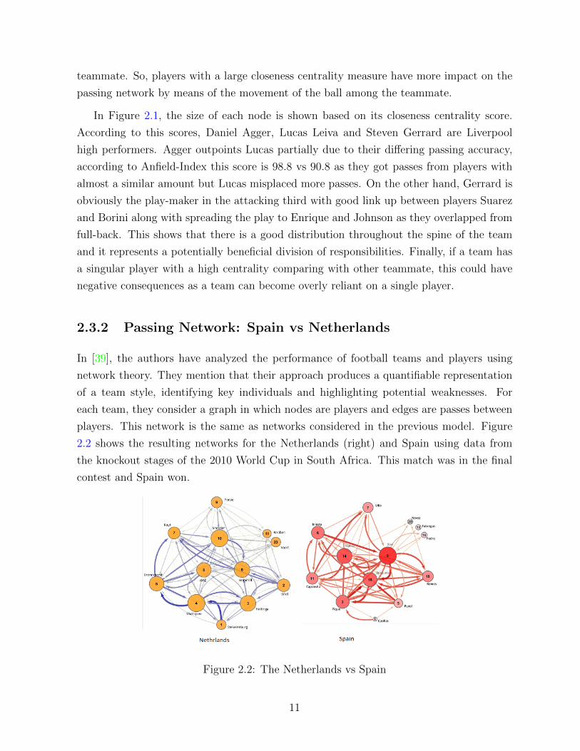
2.3.2 Passing Network: Spain vs Netherlands

In [39], the authors have analyzed the performance of football teams and players using

network theory. They mention that their approach produces a quantifiable representation

of a team style, identifying key individuals and highlighting potential weaknesses. For

each team, they consider a graph in which nodes are players and edges are passes between

players. This network is the same as networks considered in the previous model. Figure

2.2 shows the resulting networks for the Netherlands (right) and Spain using data from

the knockout stages of the 2010 World Cup in South Africa. This match was in the final

contest and Spain won.

Figure 2.2: The Netherlands vs Spain

11

An immediate result from a visual inspection of these network implies that the thickness

of the arrows indicates the number of passes between players and clearly the Spanish team

pass more often. This image captures 417 passes by the Spanish team versus 266 for the

Netherlands, data captured from the knockout stages of the 2010 World Cup. By this

data, most significant players who played and received the ball are players number 16

Sergio Busquets and number 8 Xavi, as they stand by the number of passes they make and

receive.

Let us look at some important measures of the network. In graph theory, for a given

node, roughly speaking, the closeness centrality measures how easy it is to reach the node

in the graph. In passing network terminology, it measures how well connected a player is

in the team. In the Spain team, Busquets and Xavi have the highest scores. In fact, if we

compare their scores with the rest of the players in both teams, we see that both are better

connected than the best connected Dutch player, player number 1 Steckelenberg, the goal

keeper. From the data, we see that the goal keeper is the Netherland best connected player

itself is quite revealing.

Betweenness centrality is another important indicator in analyzing networks. In graph

theory, this measures the extent to which a node lies on a path to other nodes. If we want

to interpret this measure in football passing network, betweenness centrality measures how

the ball flow between players depends on another player. So, by this definition, we can

conclude that if some players have a high betweenness centrality score, then they have a

significant impact on the structure of the network and in fact such players are fundamental

keys for keeping the momentum of the game going. In fact, these players are playing

important roles in the pitch, because removing them from the network can change the

team from high performance to low performance. Hence, if a team has a single player

with a high betweenness centrality, it would be a weakness, since it is most likely such

unique player receives a red card or is injured during entire match. In the Spain team,

player number 11 Joan Capdevilla is the one with the highest betweenness centrality in

this match. Again, by looking at the figure, one can realize that many players pass the

ball to Capdevilla who feeds mainly to player number 14 Xabi Alonso.

The other important measures in a social network is PageRank. Roughly speaking, this

invariant measures popularity of a player in terms of the number of passes he receives from

other popular players. Using data from FIFA 2010, it shows Xavi has highest PageRank

in this match. It means that after a reasonable large number of passes among all players

in both teams, Xavi is most likely to end up with the ball.

12

2.3.3 Limitations of Passing Network

As we saw in this section, many studies have been done for analyzing passing network and

all of them are based on static network. As such a network has static nature, some data is

missed, is not available or is not accurate enough in order to get high proficiency measures

of all invariants of the network. In addition, the position of nodes and the structure of

the network is built based on the a-priori ideal formation, which is not preserved during

the match. In this direction, in order to get more accurate measures from the network,

there are some suggestion such as counting the number of shots toward opponents goal by

adding an extra node for each team. Furthermore, using a similar approach to measure

the accuracy of passes by taking into account the probability of pass from one player to

another being successful, see [39, 41] for more details.

2.4 Conclusions

In this chapter we reviewed the few available studies on football passing networks done so

far. All these studies are based on a static representation of the match. In the subsequent

Chapters we will indicate the parameters and measure that we intend to study and we will

take a more dynamic approach by sliding the time of a match into windows of different

sizes and performing a more accurate time-dependent study.

13

Chapter 3

Social Network Analysis

Analyzing social networks relies on concepts of graph theory. In order to study a network

and its measures, one needs to know fundamental topics in graph theory. In this chapter,

some significant measures of social networks will be presented. We first provide some

fundamental terminologies and definitions in graph theory based on [18, 44] which will be

used frequently throughout the thesis. Some examples of graphs in social networks are

illustrated.

3.1 Some Graph Concepts

In the following section, the main terminology and the basic definitions are given for

directed and undirected graphs.

3.1.1 Simple and directed graphs

A simple graph G = (V,E) consists of two finite sets V and E of vertices (nodes) and edges,

respectively, where E is set of 2-element subsets of V . So, each edge is a 2-subset e = {u, v}of vertices joining one vertex to another. The vertices u and v are called endpoints of edge

e. In a simple graph G = (V,E), if E is a subset of E ⊆ V ×V instead of 2-element subsets

of V , then G is called a directed graph. In this case, the elements of E are sometimes called

arcs or arrows. An arc e = (u, v) consists of initial endpoint u and terminal endpoint. An

arc (u, u) is called a loop of the graph. There are two significant differences between simple

and directed graphs. In simple graphs, there are no loops and edges have no direction. The

degree of graph G is the number of vertices |V |. If G is a directed graph, for a given vertex

14

u, Γin(u) (Γout(u), resp.) is defined as the set of nodes v in which (v, u) ((u, v), resp.) is an

arc (edge)in G. The number |Γin(u)| (|Γout(u)|) is called the in-degree (out-degree, resp.)

of u. Note that for simple graphs, Γin(u) = Γout(u) and so |Γin(u)| = |Γout(u)|. We denote

this unique number by |Γ(u)| and we call it the degree of u.

One important and fundamental concept in graph theory is the one of isomorphism.

Let Gi = (Vi, Ei), i = 1, 2, be two graphs. A bijection map f : V1 7−→ V2 is called an

isomorphism from G1 to G2 if it satisfies the property: any two vertices u and v are

adjacent in G1 if and only if f(u) and f(v) are adjacent in G2. If there is an isomorphism

between G1 and G2, then we say that G1 is isomorphic to G2, denoted by G1 ' G2.

All measure measures in two graphs which are isomorphic would be preserved under

an isomorphism. For instance, the degrees of u and f(u) are the same, where f is an

isomorphism. In the following section, we will see that the characteristic polynomials of

two isomorphic graphs are the same. This is one significant observation from algebraic

graph theory point of view which enable us to explore the indicators of networks.

3.1.2 Adjacency matrix and characteristic polynomial of graphs

For a given graph G = (V,G), the adjacency matrix A = A(G) of G is defined as a square

matrix n × n, where n is the number of vertices of G, with (u, v)-entry equal to 1 if the

vertex u is adjacent to v, and equal to 0 otherwise. Note that if G and G′ are isomorphic,

then the connection between their adjacency matrices are as follows: there is an n × n

permutation matrix P such that

P−1A(G)P = A(G′).

Note that if we apply a trace function on both sides of the above equality, then trA(G) =

trA(G′). The characteristic polynomial χG(x) of G is defined by:

χG(x) = det(xI − A(G))

A walk in a graph is an alternating sequence of vertices and arcs:

u0, e1, u1, e2, u2, . . . , em, um

where et is the arc (ui−1, ui). A path is a walk with no repeated vertices or edges. The

length of the latter walk is m and starts at u0 and ends at um. Now we describe the

15

relationship between characteristic polynomial and walks in a graph. If u0 = um, then the

walk is called a closed walk. Walks of length zero are allowed, for each vertex u there is

only one such walk starting at u. In the following lemma, by using the adjacency matrix

of a graph we can find the number of walks between any two given vertices.

Lemma 3.1.1 [18, 2.1 Lemma] Let G be a graph with adjacency matrix A and let u and

v be vertices in G. Then the number of walks in G from u to v with length m is equal to

(Am)uv. The number of closed walks of length m in G is equal to trAm, where tr is the

trace function.

A simple graph G is connected if for every pair of vertices u and v, there exits a path

from u to v, otherwise, it is called disconnected. A largest connected subgraph of G is

called a connected component of G. If G is a directed graph, it is called strongly connected,

if for every pair of vertices u and v, there is a directed path from u to v and a directed path

from v to u. The strong connected component of G is a largest strongly directed subgraph

of G.

3.1.3 Eigenvectors of graphs

In this section we explain a very useful way of studying eigenvectors of a graph. Suppose

that G = (V,E) is a graph and A = A(G) is its adjacency matrix. Let X be an eigenvector

of A with eigenvalue λ. Since A is a (0, 1) matrix, the equation AX = λX is equivalent to

the following system of linear equations:

λxv =∑u∈Γ(v)

xu, v ∈ V (3.1)

From the above equations, we can get a useful interpretation for eigenvector as follows: look

at X as a vector from V to the real numbers, i.e., X : V 7→ R, then these equations imply

that λ times of the function X at u-th component is nothing but the sum of components

of X on the neighbors of u. Conversely, any real value function on vertex set V of G which

satisfies equalities 3.1 can be seen to be an eigenvector. In fact, by looking at eigenvectors

in this way, we find that such a real map provides a weighted map on the vertices of the

graph. Suppose that λ is an eigenvalue of the adjacency matrix A of G with multiplicity

k. So, the dimension of the eigenspace W corresponding to λ is equal to k. Now, let B

be an n × k matrix with its columns forming a basis for W . Then it is easy to see that

AB = λB. This implies that the rows of B give rise to a vector valued function b, on the

16

vertex set of G such that λb(u) is equal to the sum of the values of b on the neighbors of

u. Conversely, if a vector valued function satisfies the latter conditions, it determines an

eigenspace of A.

We illustrate the above argument for the cube in R3, seen Figure 3.1. Each vertex of

the graph corresponds to the vector with all entries ±1. Two vertices are adjacent if and

only if the corresponding vectors differ in only one position. As we see, if we sum the

vectors adjacent to a given vector X, the result is exactly X. Hence, by looking at the

vectors adjacent to (−1, 1, 1), we get

(1, 1, 1) + (−1,−1, 1) + (−1, 1,−1) = (−1, 1, 1)

Figure 3.1: The cube in R3

3.1.4 Union graphs and its characteristic polynomials

Suppose that Gi = (Vi, Ei), i = 1, 2 is a graph. The union of G1 and G2 is defined as the

graph G = (V,E), where V = V1∪V2 and E = E1∪E2. Just by definition of characteristic

polynomial of graph, it is easy to see that

χG(x) = χGi(x)χG2(x). (3.2)

17

3.1.5 Perron-Frobenius theorem

As we know, if C is an arbitrary n×n matrix then its eigenvalues can be complex numbers.

The spectral radius of C, denoted by ρ(C), is defined by the non-negative real number

max{|λ| : λ is an eigenvalue}. Suppose that D is a matrix. We write C ≥ D where D is a

matrix such that C−D exists and is non-negative. For a given arbitrary square matrix C,

we may define the underlying directed graph corresponding to C as a directed graph whose

adjacency matrix is obtained by replacing each nonzero entry of C with 1.

Theorem 3.1.2 (Perron-Frobenius theorem) Suppose that C is a non-negative n× n ma-

trix such that its underlying directed graph is strongly connected. Then the following state-

ments hold:

(a) The spectral radius ρ(G) is a simple, non-zero, eigenvalue of C, and the corresponding

eigenvector can be taken to be positive.

(b) Let λ1, . . . , λk be all the eigenvalues of C with absolute value equal to λ. Then k > 1

if and only if all closed walks in G have length divisible by k. For all i, λi/λ is a k-th

root of unity.

(c) If D is an n × n matrix with |D| ≤ C, then ρ(D) ≤ ρ(C), with equality if and only

if D = ±C.

We will use the Perron-Frobenius theorem in order to measure a significant indicator in

social network, namely eigenvector centrality.

3.2 Social Network Analysis

The study of the relationships between social entities can be done by means of social

networks. In the sport world, any football match establishes a social network called football

passing network in which relationships are passes among players as entities of a team. Social

network analysis deals with the structural analysis of networks. For instance, analyzing

the football passing network gives us information about how a player involves with the

others (local level) or how a team has performed (global level).

We give a brief overview of important measures of networks which will be used in

analyzing the passing networks.

18

3.2.1 Node centralities

One of most important indicators in analyzing network is degree which is used as a first

step when studying a network, see [16, 32, 45]. To mathematically describe this indicator,

let X be the adjacency matrix of a network G = (V,E) under study and u ∈ V be a node.

Then the degree of u is given as follows:

ku = CD(u) =∑v∈V

Xu,v. (3.3)

Note that this is true only for an undirected and binary network, it means that Xu,v = Xv,u,

for all u, v ∈ V and Xu,v = 1 if u and v are neighbors otherwise Xu,v = 0.

In weighted network, the degree of a node u has generally been extended to the sum

of weights of edges e in which e meets u, and labeled node strength, see [37, 35]. Node

strength has been formalized as follows:

su = CWD (u) =

∑v∈V

Wu,v (3.4)

where W is the weighted adjacency matrix of the network. If the network is binary,

each edge has weight 1, then this definition is equal to the definition of degree. On the

other hand, in weighted networks, the outcomes of two measures given in (3.3) and (3.4)

are different. In weighted networks, in order to analyze the network, the node strength

has been preferred as a measure since it takes into consideration the weighted edges, see

[36, 37]. In fact, node strength is a straight measure as it calculates the node’s total degree

of involvement in the network and not the number of nodes that connected to it. In Figure

3.2, node 2 and node 3 have the same strength, but node 2 has twice as many neighbors

as node 3. It implies that node 2 is participated in more parts of the networks.

We note that degree and strength are both measures of the level of involvement of a

node in the network. So, when analyzing the centrality of a node, it is important to identify

both these measures.

In order to combine both degree and strength, we use an adjustment parameter α

which indicates the relative significant of the number of edges compared to edge weights.

Precisely, a degree centrality measure is proposed by the product of the number of nodes

that a focal node is connected to and the average weight to these nodes adjusted by the

adjustment parameter, see [36]. The following formula gives a formal definition for a degree

centrality measure:

19

Figure 3.2: A weighted network with 8 nodes. The thickness of edges correspond to theirweights

CwαD (i) = ki ×

(siki

)α= k

(1−α)i × sαi (3.5)

where α is a positive real number that can be set according to the setting and the data.

If 0 ≤ α ≤ 1, then high degree would be preferable , whereas if 1 < α, a low degree is

favourable.

So far, we discussed undirected network, i.e., links without direction. Since, we would

analyze directed and weighted network, let us consider the degree centrality measure in a

directed and weighted network. In this case, two additional aspects of a node’s involvement

are added to identify the degree measure. The activity of a node or its social role can be

quantified by two measures as follows: the number of edges that are directed towards the

node, denoted by kin, is a representative of its popularity, the number of edges that originate

from the node, denoted by kout. Since not all edges are not reciprocated, in general kout is

not equal to kin. The strength of a node is involved with two measures: sinu (resp. soutu ) is

the total weight attached to incoming edges (resp. outgoing edges). These two measures

have the same limitation as s, i.e., the number of edges are not considered. The following

two measures are proposed to access a node’s activity and popularity, respectively

CwαDout

(u) = koutu ×(soutu

koutu

)α(3.6)

CwαDin

(u) = kinu ×(sinukinu

)α(3.7)

The adjustment parameter α is the same as the one in Equation 3.4. If two nodes have the

same sout and different kout, the measure would assign a higher score to the node with the

20

highest kout if α < 1, whereas if α ≥ 1 the measure would assign a highest score to node

with lowest kout. For more information we refer the reader to [36].

3.2.2 Closeness and betweenness centralities

The closeness and betweenness measures depend on recognition and length of the shortest

paths among nodes in the network. In order to generalize these measures for weighted

networks, we need to know how to generalize the shortest distances and their length from

binary to weighted networks. In [24, 34, 40, 45, 48] there have been results about the

shortest distances among nodes in binary networks. In a binary network, the shortest path

between two nodes A and B is defined as the minimum of the length of all path between A

and B. Clearly, the length of a path is the number of edges connecting any two consecutive

nodes in the path. If there are many intermediary nodes between A and B on a path that

connects A to B, the cost of interaction between these two nodes increases. Moreover, the

intermediary nodes can slant information or delay interaction between nodes, see [7, 17].

Clearly, in binary networks the shortest path between A and B is the smallest number of

intermediary nodes.

There are different aspects of the shortest distances among nodes in a network such

as the all-pairs shortest- path and the single-source shortest-path problem. Closeness

centrality relies on the single-source shortest-path, i.e., the length of the shortest path from

one node to all other nodes, whereas betweenness relies on the identification of the all-pairs

shortest-path, i.e., the lengths of shortest paths between all possible source-destinations

pairs.

The definition of closeness and betweenness in an undirected and unweighted network

is given in [15] as follows, respectively:

CC(u) =

[∑v∈V

d(u, v)

]−1

(3.8)

CB(u) =∑

v 6=w∈V \{u}

Pvw(u)

Pvw(3.9)

where d is the distance function, so d(u, v) is the length of the shortest path between node

u and node v, Pvw is the number of shortest paths from v to w and Pvw(u) is the number

of those paths that go through node u.

21

It is more complicated if we want to calculate these two measures for weighted networks.

For instance, data can be transmitted though a longer path of strong link more quickly,

and diseases have higher probability to carry on through a sequence containing individuals

through strong links than through a weak direct connection.

This situation is illustrated in Figure 3.3. In this example, we have a weighted network

with three paths between two nodes, node 1 and 3 which are connected through three

different paths with different number of intermediary nodes with different weights. If our

network in Figure 3.3 was binary, then the shortest path would be the direct connection

1− 3. However, in a weighted network, we would like to know if this path is the quickest

path for flow. Although path 1, 5, 4, 3 goes through two intermediary nodes, it could be

quicker since the path consists of stronger links.

Figure 3.3: A weighted network with three paths between two nodes: 1 and 3, directlypath 13; through one intermediary node 123; through two intermediary nodes 1543. Thethickness of edges correspond to their weights

Finding shortest paths in weighted networks has been studied in [10, 24, 40, 48]. For

instance, in [10] the author proposed an algorithm that finds the shortest path for networks

in which the weights are identified as cost of transmitting, e.g., time to route Internet traffic

or distances in GPS devices. In reality, in most cases weights are considered based on edge

strength not on their cost, in which case the edge weights must be reversed before directly

applying Dijkstra’s algorithm to find the shortest paths. In [34] the author has proposed

to invert the weights in order to generalize closeness and betweenness centralities. To do

so, weights on each edge are considered as costs since large value on each edge represented

weak or costly edge, whereas small value on each edge identifies strong or cheap edge.

For example, if edge < A,B > has weight 2 and edge < C,D > has weight 1, then the

distance between A and B is half of the distance between C and D. If there is no path or

edge between two nodes, then the distance would be considered as infinite number. More

22

precisely, the distance function for a weighted network for implementation of Dijkstra’s

algorithm is defined as the following:

Dw(u, v) = min

(1

Wuu1

+1

Wu1u2

+ . . .+1

Wukv

)(3.10)

where minimum is taken over all path < u, u1 >< u1, u2 > . . . < uk, v > from u to v. In

this model, the number of intermediary nodes are not considered, so the distance between

two nodes is not affected by the number of nodes that lie on the path connecting them.

Opsahl and et al., by following ideas from [10, 34], have extended the shortest path

algorithm by taking into consideration the number of intermediary nodes. They transform

the inverted weights by a similar adjustment parameter used in the formula for degree

measure. Equation 3.5 is used to find the least costly path before applying Dijkstra’s

algorithm. Using an adjustment parameter grantees that both weight and the number

of intermediary nodes affect the determination of shortest paths. So, from the above

argument, the length of the shortest path between two nodes is defined as follows:

Dwα(u, v) = min

(1

(Wuu1)α

+1

(Wu1u2)α

+ . . .+1

(Wukv)α

)(3.11)

where α is a positive real number which is called tuning parameter (see [36]).

By combining Equations 3.11 and 3.8 the centrality measure in weighted networks is

provided in [36] as follows:

CwαC (u) =

[∑v∈V

Dwα(u, v)

]−1

. (3.12)

Furthermore, it is possible to extend betweenness centrality by taking advantage of the

defined shortest path algorithm. To do so, by combining the weights on edges and the

number of intermediary nodes, betweenness centrality is given as follows:

CwαB (u) =

∑v 6=w∈V \{u}

Pwαvw (u)

Pwαvw

. (3.13)

Now, we have a generalization of betweenness and closeness centralities from simple net-

works to weighted networks. Since we would like to analyze directed and weighted networks,

we need to generalize the betweenness and closeness centrality to directed and weighted

networks. In fact, the calculation of the shortest paths and their length in directed net-

works can be done in the same way as in undirected networks with a constraint. In order

23

to find the length of a path from one node to another, we should follow the direction of the

corresponding edges. For example, in road networks, the car can move from one direction

to reach location B from location A. This implies that the distance from node A to B is

not necessarily equal to the distance from node B to node A.

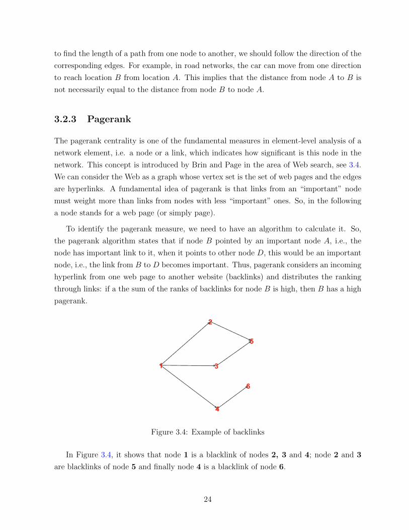
3.2.3 Pagerank

The pagerank centrality is one of the fundamental measures in element-level analysis of a

network element, i.e. a node or a link, which indicates how significant is this node in the

network. This concept is introduced by Brin and Page in the area of Web search, see 3.4.

We can consider the Web as a graph whose vertex set is the set of web pages and the edges

are hyperlinks. A fundamental idea of pagerank is that links from an “important” node

must weight more than links from nodes with less “important” ones. So, in the following

a node stands for a web page (or simply page).

To identify the pagerank measure, we need to have an algorithm to calculate it. So,

the pagerank algorithm states that if node B pointed by an important node A, i.e., the

node has important link to it, when it points to other node D, this would be an important

node, i.e., the link from B to D becomes important. Thus, pagerank considers an incoming

hyperlink from one web page to another website (backlinks) and distributes the ranking

through links: if a the sum of the ranks of backlinks for node B is high, then B has a high

pagerank.

Figure 3.4: Example of backlinks

In Figure 3.4, it shows that node 1 is a blacklink of nodes 2, 3 and 4; node 2 and 3

are blacklinks of node 5 and finally node 4 is a blacklink of node 6.

24

In [38] a slightly simplified version of pagerank is given as follows:

Pr(u) = α∑

v∈Rin(u)

Pr(v)

|Rout(v)|(3.14)

where u represents a web page and α is a factor used for a normalization.

From 3.14, we see that the rank score of a page u is obtained recursively based on score

of all pages that point to u. In fact, this rank can be calculated iteratively starting from

any webpage and it does not depend on any particular page. It might be possible within a

webpage to have two or more pages connected to each other to make a loop. If these pages

are referred by other pages outside the pages of the loop, and they did not refer to any

page outside the loop, they would never propagate any rank but they would accumulate

rank. This process is called rank sink, see [38] for more information.

The original pagerank is given in 3.14 based on the rank sink problem as follows:

Pr(u) = (1− d) + d∑

v∈Rin(u)

Pr(v)

|Rout(v)|(3.15)

where d is a dampening factor and normally is set to 0.85.

Mathematically, we can define the pagerank vector pr(α, s) of a network G as the

unique solution of the following system of linear equations:

pr(α, s) = αs+ (1− α)pr(α, s)W (3.16)

where α ∈ (0, 1] is a jumping constant; s = 1n1 is a starting vector and W = (wij) as

follows wij = 1di

, if node i adjacent node j, otherwise wij = 0.

In [47], pagerank is generalized to weighted networks as follows:

Pr(u) = (1− d) + d∑

v∈Rin(u)

Pr(v)W in(v,u)W

out(v,u) (3.17)

where W in(v,u) and W out

(v,u) are the popularity from the number of in-links and out-links,

respectively. More precisely, W in(v,u) is the number of in-links of page u out of the number

of in-links of all reference pages of page v:

W in(v,u) =

|Rin(u)|∑p∈R(v) |Rin(p)|

25

where R(v) denotes the reference page list of page v. Similarly, W out(v,u) is the number of

out-links of page u out of the number of out-links of all reference pages of page v:

W out(v,u) =

|Rout(u)|∑p∈R(v) |Rout(p)|

Interpretation of Pagerank in Football Network

As we mentioned in previous section, pagerank centrality is a recursive notion of popularity

when a node is referred by other popular node in the network. Following 3.16, we extract

an exact formula for pagerank centrality xi of each node i as follows: Let pr(α, s) =

(x1, x2, . . . , xn) be the pagerank vector associated with search ranking vector s = 1n1.

From 3.16 we have

pr(α, s) = (x1, x2, . . . , xn) = α1

n1 + (1− α)(x1, x2, . . . , xn)W.

This implies that

xj =α

n+ (1− α)

∑t: t→j

1

dout(t)xt (3.18)

where t→ j means that there is a directed link from t to j.

From 3.18, we see that PageRank is an eigenvector algorithm which assigns scores to

each node. The score for a given node may be considered as the fraction of time spent

”visiting” that node (measured over all time) in a random walk over the nodes (following

outgoing edges from each node). Pagerank modifies this random walk by adding to the

model a probability, indicating by a parameter α in 3.18 of jumping to any node. From 3.18,

it is easy to see that if α = 0, this is equivalent to the eigenvector centrality algorithm.

On the other hand, if α = 1, all vertices will receive the same score 1/|V |. Therefore,

parameter α acts as a sort of score smoothing parameter.

Let α = 1 − p and q = 1−pn

, then from 3.18 we conclude the following formula xj for

each node j

xj = q + p∑t: t→j

1

dout(t)xt. (3.19)

In the case of Football passing networks, the interpretation of pagerank formula 3.19 is as

follows: dout(t) is the total number of passes made by player t; p is heuristic parameter

indicating the probability that a player will pass the ball away rather than keep it and

go for a shot by himself. Finally, q is a parameter proportional to the probability that

26

a player will shoot the ball away rather than pass it to other player. According to the

recursive formula given in 3.19, the pagerank score of a player depends on the scores of

all his teammates. This implies that all pagerank scores in a team should be calculated

simultaneously.

Roughly speaking, the pagerank centrality assigns to each player the probability that

he will get the ball after a reasonable number of passes have been made by all players in

the team. The value of probability p is not created by the team alone, as it can be different

from one team to another, and that is why p must be determined by heuristics. As a proof

of concept, in our analysis we might apply a uniform value p = 0.6, then q = 1−0.611

= 0.036.

for all the teams studied.

3.2.4 Eigenvector centrality

There is another centrality measure in networks, proposed by Peter Gould [19], that is

more sophisticated than the degree centrality, called eigenvector centrality. It is a measure

of the influence of a node in a network. Roughly speaking, the eigenvector centrality of a

node is the sum of its connections to other node in network, weighted by their centrality.

By using the adjacency matrix of a network, we can identify eigenvector centrality of all

nodes in the network. Suppose that G = (V,E) is a graph and A = (auv) is its adjacency

matrix, so auv = 1 if u is a neighbor of v, otherwise auv = 0. Define a new matrix B = A+I,

simply by replacing the diagonal zeros with ones. This has the effect of giving an eigenvalue

λ of B, then λ− 1 would be an eigenvalue of A with the same corresponding eigenvector.

Since A is a symmetric matrix, B is so and it can be diagonalized by an orthogonal matrix.

This implies that the eigenvalues of B are real and we can select the largest one. Now

we check the requirement of Perren-Frobenius Theorem 3.1.2. We remind the reader that

a matrix D = (d(u, v) us is called non-negative if d(u,v) ≥ 0 for all u, v. A non-negative

matrix D is called primitive if there exits an integer N > 0 such that every entry in DN is

strictly positive.

To check the hypothesis of Perron-Frobenius Theorem 3.1.2, we calculate Bk, where

k is a positive integer number. Let us see what is the (u, v) entry of matrix Bk. In

fact, (Bk)uv is the number of ways traversing from node u to node v by walks of length k

including stopover. Since the diameter diam(G) of a connected graph is the smallest integer

k such that any two nodes u, v can be connected by a walk no longer than k, if we chose

k ≥ diam(G) then Bk would be positive. Therefore, B is primitive and all requirements in

3.1.2 are satisfied.

27

The above argument ensures that for a connected graph, we can find a principle vector

v0 whose entries are all positive. Let λ0, λ1, . . . , λn be all eigenvalues of B with eigenvectors

v0,v1, . . . ,vn, respectively. Take the following linear combination of eigenvectors which is

clearly not orthogonal to v0:

v = α0v0 + α1v1 + · · ·+ αnvn, (α0 6= 0).

Since each λi is an eigenvalue with corresponding eigenvector vi, we get

Bkv = λk0α0v0 + λk1α1v1 + · · ·+ λnαnvn.

This implies thatBkv

λk0= α0v0 +

λk1α1v1

λk0+ · · ·+ λknαnvn

λk0.

By taking limit from both sides of the above equation, when k →∞, we get Bkvλk0→ α0v0,

it holds because λ0 > λi, i 6= 0. We conclude that when k is increasing, the ratio of all

components of Bkv tends to corresponding components of v0.

By the above argument, entry v in row u determines all k length walks from node u to

node v. It shows that the row sum is the total number of k-length paths to all other nodes

from node u. If v = 1, the vector with entries are 1, the row sums of Bk are exactly equal

to Bkv. As we saw in the above, counting longer and longer paths would lead us to bring

Bkv to the same ratio as eigenvector centrality.

Therefore, in oder to formalize the eigenvector centrality of nodes we use the above

discussion and we can define the centrality score as an eigenvector v corresponding to the

largest eigenvalue λ as follows: Av = λv. We can find exact value of scores for every node.

Let X = (xv)v∈V be the eigenvector corresponding to the largest eigenvalue λ mentioned

above. Then the solution of the system of linear equation AX = λX is as follows:

xv =1

λ

∑u∈R(v)

xu =1

λ

∑u∈V

Avuxu. (3.20)

In equation 3.20, λ is the largest eigenvalue and all entries of X are positive. The uth

component of the related eigenvector gives the centrality score of the node u in the network.

In the above we explained how to achieve the centrality scores by power iteration. This

process is one of many eigenvalue algorithms that can be used to obtain this dominant

scores.

28

3.2.5 Clustering coefficient

To analyze a social network there is another measure called clustering coefficient. In undi-

rected networks, it is a measure of the number of triangles in a graph. In [46], the concept

of clustering coefficient have been proposed for unweighted and undirected networks and

Fagiolo in [11] has generalized it for binary directed and also weighted directed networks.

Let G = (V,E) represents a weighted and directed graph. Let A be adjacency matrix

of G whose entries are 0 and 1 and let W be adjacency matrix of G whose entries represent

weights on edges. Define dinu = |Rin(u)|, doutu = |Rout(u)| as in-degree of node u and out-

degree of node u. Let du = dinu + doutu be the total degree of node u and let

d↔ =∑

u6=v∈V

AuvAvu.

If W = A, i.e., G is a binary network, then the clustering coefficient of node u is defined

as the ratio between all the possible triangles formed by node u and the total number of

triangles that could be formed:

CDu =

(A+ AT )3uu

2[du(du − 1)− 2d←→u ]. (3.21)

The above formula can be easily extended to the wighted directed graph as follow:

CWu =

(W + W T )3uu

2[du(du − 1)− 2d↔](3.22)

where W = (w13uv). In [11] it is mentioned that the above definitions 3.21 and 3.22 are

not characterizing the richness of patterns that take place in a complex directed network.

The reason is that Equations 3.21 and 3.22 consider all possible triangles without their

directions. However, in directed graph we should consider the direction edges in underline

triangles. So, in order to remove this problem, four more definitions are treated as shown

in the following:

Case (a): cycle, consider a directed cycle started at node A. In this case, the associated

clustering coefficient is given as follows:

Ccycu =

(W )3uu

dinu doutu − d←→u

. (3.23)

29

Figure 3.5: classification of the triangles based on directed networks

Case (b): Middleman, one of the adjacent node of A has out-degree of 2 and other has

in-degree of 2. In this case, the associated clustering coefficient is given by the following:

Cmidu =

(WW T W )uudinu d

outu − d←→u

. (3.24)

Case (c): node A has in-degree of 2. The clustering coefficient is given by the following:

Cinu =

(W T W 2)uudinu (dinu − 1)

. (3.25)

Case (d): out, the out-degree of node A is equal to 2. The clustering coefficient is as

follows:

Coutu =

(W 2W T )uudoutu (doutu − 1)

. (3.26)

3.3 Conclusions

In this Chapter we discussed all the measures that we intend to use for the analysis of

a specific dynamic passing network corresponding to a World cup match between the

Netherlands and Spain: degree centrality, closeness, betweenness, page rank, and clustering

coefficient.

30

Chapter 4

Time-Varying Graphs

A vast majority of real-world networks are dynamic (or time-varying or evolving) as op-

posed to static. In the past few years, intensive research effort has been devoted to study

dynamic graphs. Since the study of dynamic graphs is a relatively new research area, the

concepts and definitions are not well-developed yet, and the same concept, sometimes, is

referred to by different terms. For instance, there is not even a common terminology on

naming the concept of graphs that change over time. For example, Kempe et al. [25]

uses the term temporal network, while Leskovec et al. [29] refer to them as graphs over

time; Flocchini et al. [13] employ the term time-varying graphs (TVG). In this Section we

introduce the notion of time-varying graphs and the main definitions around the concept

of graphs that change over time.

4.1 Definitions

The need for dynamics-related concepts emerged from a range of very different investiga-

tions. In fact, dynamic networks play an important and central role in a variety of research

areas. For instance, delay-tolerant networks (DTNs), highly-dynamic, infrastructure-less

networks whose essential characteristic is a possible absence of an end-to-end communica-

tion route at any instant, are an exact mapping for dynamic networks [22, 21, 31, 42, 43, 49].

While DTNs mostly focused on fixed network objects, researches on moving network objects

continued with studying opportunistic-mobility networks [50, 1, 6, 9]. Dynamic networks

have also been an interest in complex systems [28, 26]. Our focus is the application of

TVGs in dynamic football passing networks.

Time varying graphs have been defined in [8] and they constitute a general framework

31

to describe dynamic networks. We give their formal definition below.

Definition Let G be a system consisting of a set of units V and set of pairs E of units

interacts with each other, over a time interval T, called lifetime of system G. If the system

G under study runs over discrete (continuous, resp.) time, then T is s subset of N (R+,

resp.). Then the quintuple G = (V,E,T, ρ, ζ) is called time varying graph, abbreviated by

TVG, where E ⊆ V × V is the set of edges in such a way that (u, v) ∈ E if and only if u

has at least one interaction with v at time t ∈ T, and

ρ : E ×T −→ {0, 1}

is a map indicating whether a given edge exists at a given time; the latency function

ζ : E×T −→ T indicates the time it takes to cross a given edge if starting at a given date.

In this thesis, we assume that the temporal domain T is discrete (the unit of time

is given by a second) and finite. It means that we focus on systems with finite lifetime,

namely T = [t0, tk], where t0 < tk are positive real numbers. When the interaction between

nodes are directed, it means that our binary relation E on V gives us ordered pairs (u, v);

pair (u, v) indicates an interaction from node u to node v.

Example Let us provide several examples of both directed and undirected TVGs as fol-

lows:

• Friendship network. In social networks, the friendship relation between people gen-

erates a time varying graph in which the underlying graph is simple. In this network,

in the most general sense of the term, the set of nodes is a group of people, and

edges are defined by social interactions or ties of some kind. This is an example of

undirected TVG.

• Transportation networks. In this system nodes are cities, and directed edges are, for

example, flights whose departure dates are given by punctual presences. This is a

directed TVG.

• Wireless mobile networks. This is a well known example of communication networks,

where an edge is present whenever its two endpoints are within range. This gives us

an undirected TVG.

32

• Scientific networks. In this social network, nodes are researchers in a specific branch

of science, and edges are coauthors. Clearly, this network provides an undirected

TVG.

The above examples demonstrate aspects of modules over which the TVG definition

can extend. As we see, some contents are simpler than others and call for limitations,

such as directed vs undirected edges or single vs multiple edges. Additional restrictions

might be considered, for instance the latency function could be determined constant over

time, over the edges, over both, or actually ignored. In fact, a vast majority of work in

social networks does not require such information (e.g., the propagation time of an email

is of little interest to the understanding of a community behavior). Since the scope of this

thesis is about analyzing a realistic social network, we will intentionally omit the latency

function.

In order to analyze the network measures during the lifetime of a time varying graph,

two types of indicators are described: atemporal and temporal ones. Atemporal parameters

are defined based on static networks and their evolution over time can be obtained by

measuring them over sequences of static graphs, where each of the sequence corresponds

to the aggregation of interactions that occur in a given interval of time, any elements of

such a sequence is called footprints of a TVG. Whereas, temporal indicators are defined

on time varying graphs in terms of their temporal nature. In this model, a sequence of

non-aggregated time varying graphs, each of which corresponds to a temporal subgraph

of the original one for the considered interval, is required for the evolution of temporal

measures. In this thesis we use atemporal indicators.

4.2 Football Passing Networks as Evolving Graphs

The notion of evolving graph introduced in [12] is the one that closely fits our description

of the dynamic football passing network. Consider the situation, in discrete time systems,

where each footprint interval corresponds to the unit of time, or to the time between any

two consecutive modification of the graph. In these cases, every footprint corresponds to

an instant snapshot of the network, and the sequence corresponds exactly to the evolving

graph model. In our setting, instead of considering a new snapshot for each network change,

we construct sequences of footprints by aggregating the time information in intervals of

time. The extreme situation would be when a single interval is considered, covering the

whole lifetime of the system, resulting in a single static footprint which is the aggregation

33

of all interactions over the network lifetime. More precisely, we will use the following,

slightly changed, definition of evolving graphs.

Definition Let T = [t0, tk] be a time interval, where t0 < tk. Partition T into subintervals

[t0, t1), [t1, t2), . . . , [tk−2, tk−1), [tk−1, tk]. For each i = 0, 1, . . . ,m, define atemporal time

varying graph Gi = (Vi, Ei) where the set of vertices and edges Ei are considered during

time subinterval [ti, ti+1). Then the triple E = (G,SG, ST ) is called an evolving graph with

respect to T, where ST is the sequence t0, t1, . . . , tk of time instance, SG is the sequence

G1, G2, . . . , Gk of the graphs Gi and G =⋃k−1

0=1 Gi. Denote E be the edge set of G.

For a given time varying graph, when considering a sequence of footprints SF that

correspond to a sequence of time intervals, we have a sequence of static graphs, and any

classical network measure, such as pagerank, centrality, betweenness, etc. can be directly

applied to each. When we look at the evolution of an measure over a sequence SF , we

might capture diverse values of granularity by modifying the size of the footprint intervals.

According to measures and applications, different choices of granularity might be better to

capture a significant behavior.

Suppose that there is a football match between two teams A and B. For teams A and

B, we define football passing network G(A) and G(B), respectively as follows: for team Anetwork G(A) is a graph in which the set of vertices is all 11 players from team A and the

set of edges is the set of links between any two players of team A. Here, a link between

player A to player B means that player A passes the ball to player B. This graph is a

directed weighted graph, with the weight being the number of passes from player A to

player B. Moreover, each edge is labeled with the time when the corresponding passes

occurred.

As we know, the duration of a football game is 90 minutes (5400 seconds), which is

divided into two 45-minute (2700 seconds) halves. Each half can be extended as decided by

the referee. This extension of the game length is called injury period or stoppage time. We

assume that a match between two teams over time interval [0, 2700] for the first half time.

Note that number 2700 is taken as 45 minutes in terms of seconds and can be extended

to 3000, for instance if there is 5 minutes extra time. Let us define the football passing

network of team A as the following:

Definition Let T = [0, t], where t is the match duration. The football passing network

G(A) of team A is an evolving graph E = (G,SG, ST ) with respect to T, where ST is the

sequence 0, t1, . . . , tk = t of time instance, SG is the sequence G1, G2, . . . , Gk of directed

34

graph Gi with a weight attached to each edge in which the set of vertices is represented as

a subset of players among all of 18 players and there is an edge from A to B with weight

w if w number of passes has been made from player A to player B and G =⋃kt=1Gi.

In the above definition, each component Gi is called aggregated football passing network

over time interval [ti, ti−1].

Remark Suppose that we would like to study the evolution of a social network over a

time interval T = [t0, tk]. Depending on the topology of social network under study, we

partition T into subintervals [t0, t1), [t1, t2), . . . , [tk−2, tk−1), [tk−1, tk]. Now, the aggregated

graph A(G) over total time interval [t0, tk] is exactly the evolving graph E = (G,SG, ST ).

Figure 4.1: letf: Aggregated football passing graph over time interval [0,88]; right: Aggre-gated football passing graph over time interval [88,176]

Figure 4.2: Aggregated football passing graph over time interval [0,176]

Figures 4.1 and 4.1 illustrate the above remark showing examples of aggregated football

passing networks corresponding to a match. In figure 4.1 there are two graphs: on the left,

let G0 is the aggregated football passing network over time interval [0, 88) and on the right,

G1 is the aggregated football passing network over [88, 176). Moreover, in Figure 4.2, we

can see the aggregated football passing network G over interval [0, 176).

35

Chapter 5

Models for analyzing dynamic

passing network

In this section, we introduce the two models on which we base our study of a dynamic foot-

ball passing network: the Aggregated Model, and the Non-Overlapping Sliding Windows

Model.

5.1 The Data

In the next Chapter we will analyze the measures described in Chapter 3 to study the

structure of a dynamic football passing network that has been extracted from the final

match between the Netherlands and Spain during World Cup 2010. The 2010 FIFA World

Cup Final was a football match that took place in Johannesburg, South Africa, to deter-

mine the winner of the 2010 FIFA World Cup. Spain defeated the Netherlands 1-0 with a

goal from Andres Iniesta four minutes from the end of extra time. The data correspond to

the passes among players in the first half of the game, and it is tagged by the time when

each pass occurred. More precisely, for each team, we created a table with three columns

called From, To and Time. Let N,M and t be numbers corresponding to From, To and

Time respectively; this means that player number N passed the ball to player number M

at time t, the time is in terms of seconds. The data has been collected based on the first

half time period of the match plus extra time considered by the referee, for a total of 2772

seconds.

36

5.2 The Aggregated Model

By nature, a football passing network is dynamic, both in terms of passes and in terms of

players involved in them throughout the match. Although the number of players in the

football team is fixed (11), this number and the interactions between the players change

over time, i.e., some players may appear in a specific time period and some of them may

not appear in that period. In such a dynamic setting, an aggregation of all data would lead

to a loss of all temporal information. An intuitive way to capture the dynamics of football

passing network is to aggregate edge weights, which represent the number of passes between

two players, only over a certain time period and extend this period to develop a discrete

notion from aggregated data. In our network where players interact through passing the

ball, the aggregation could be to sum of the number of passes over a specific time period.

So, the network is growing over time in terms of number of players and number of passes

between them. We expect that for each football team, the network under study tends to

a complete graph after a certain time. With this approach, the aggregation of the passes

over time would influence the old players in the network over players who just joint to this

subgraph.

Following this idea the aggregated model proceed as follows. The total time span of our

data is T = 2772 seconds. This time is covered in an aggregated way by using windows of

different sizes: 198, 308, 924, 1386, 2772. The “static” case correspond to a single window

of size 2772; for window size 1386 we obtain 2 periods of time [0, 1386] and [0,2772]; for

window size 924 we obtain 3 periods of time [0, 924], [0,1848], and [0, 2772] and so on for

smaller windows.

Windows Size (second) Windows Number

198 14

308 9

924 3

1386 2

2772 1

Table 5.1: Aggregating Periods Model

We construct a directed weighted graph for each team, G for Spain and H for the

Netherlands respectively, by associating nodes to players with arcs between nodes rep-

resenting passes between them. Arcs are weighted by the number of passes in the time

37

period and labeled by the times when those passes have occurred. We create two aggre-

gated graphs Gi and Hi for each period [0, i× t], where t is the window size, thus obtaining

a sequence of graphs for each team in correspondence of each window size.

Note that aggregating windows can create anomalous situations where a time period

might contain more than 11 players. This is the case when a player is substituted. Consider,

for example, the situation of player number 17, who is replaced by player 20, 40 seconds

after the start of the game; his inactive presence is recorded throughout the game and

impacts the network measures.

5.3 The Non-Overlapping Sliding Windows Model

In the aggregated model, while we are analyzing the football passing network there is a

drawback that we cannot prevent: the prevalence of players who have performed many

passes at the beginning of the match over players who have a chance to pass the ball to

other players only later during of the match. This can happen, for example, when a new

player appears in the network towards the end of a window under consideration. If we look

at this new player who was added to the network at the last moment, all his scores will be

quite low in comparison with the other players. In order to reduce this disadvantage, we

consider another approach called sliding windows. In this model, we partition the viewing

period in equidistant time windows, each window starting when the last window finished.

Windows Size (second) Windows Number

99 28

396 7

1386 2

Table 5.2: Non-Overlapping Sliding Windows Model

In our analysis, we consider 4 different window sizes as is illustrated in Table 5.2: 2772,

1386, 396, 99 corresponding to a single time period of the total time of the match (2772

sec.), 2 consecutive periods of 1386 sec. each, 7 consecutive periods of 396 sec. each, 28

consecutive periods of 99 sec. each.

After specifying the interval for each time window, we create a directed weighted graph

Gt based on the observations made during that period, where t shows the time interval

over which the information is captured. For example, for window size = 99 there are 28

windows. According to the first window, two aggregated graphs G0 for Spain and H0 for

38

Spain over time interval [0, 99] are created. For the second window, an aggregated graph

G1 for Spain and H1 for the Netherlands are established over time interval [99, 198]. For

the third window, two aggregated graph G2 and H2 are built over time interval [198, 396],

and so on. Finally, for the last window, aggregated graphs G27 and H27 are built over time

interval [2673, 2771].

5.4 The Study

In the next chapter, we focus on degree, closeness, betweenness, pagerank, eigenvector

centrality and clustering coefficient in two models described above. More precisely, we will

compute these measures for each player and for each set of time windows corresponding

to the various different ways of dividing the overall time of play. For example, in the non-

overlapping windows model with window size 396, we have 7 windows corresponding to 7

consecutive periods and 7 passing networks. For each player, we compute the six measures

indicated above for each of 7 time periods and we average them. We then obtain a table for

each team indicating the average score of each player during the match for that particular

choice of window size. Finally, the measures of a single snapshot network is also computed

and compared with the average scores obtained over window times.

The data has been collected based on a close inspection of the match. The data has

then been adapted to be imported into Gephi [2] a tool for the analysis of social networks

that has a pre-defined set of network parameters already available. The various parameters

investigated in the thesis have been computed using this tool.

5.5 Conclusions

In this chapter, we defined the two models on which we base our study. In the next two

chapters we perform the analysis on the aggregated and on the non-overlapping window

model, respectively.

39

Chapter 6

Dynamic Passing Networks in the

Aggregated Model

In this chapter, we analyze some measures for dynamic passing networks, such as degree

centrality, betweenness, closeness, pagerank, eigenvector centrality and finally clustering

coefficient in the aggregated model.

We remind that in the aggregated model, the overall time is divided in growing windows

of different sizes: 198, 308, 924, 1386, 2772. The “static” case correspond to a single

window of size 2772; for window size 1386 we have 2 time intervals: [0, 1386] and [0,2772];

for window size 924 we have 3 time intervals: [0, 924], [0,1848], and [0, 2772], finally, for

window size 198, we have 14 growing time intervals.

6.1 Degree centrality in the Aggregated Model

One of the most important scores in networks is degree centrality. This score indicates

how many balls a specific player received or passed from or to other players. If a player

has a high degree it means that the player has high impact in the team in terms of the

number of his neighbors regardless of whether the other players are passing the ball to him

(in-degree) or are receiving the ball from him (out-degree). To consider the total number

of passes done by each player, we therefore use formulas 3.6 and 3.7 defined in Chapter 3

with adjustment parameter α = 1 and with strength equal to the degree.

Table 6.1 and 6.2 contain the result of the experiment for the two teams, each column

containing the average degree for a given window size.

40

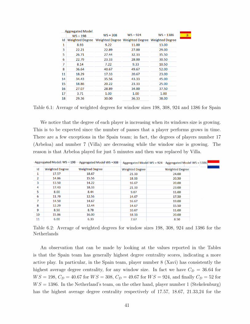
Table 6.1: Average of weighted degrees for window sizes 198, 308, 924 and 1386 for Spain

We notice that the degree of each player is increasing when its windows size is growing.

This is to be expected since the number of passes that a player performs grows in time.

There are a few exceptions in the Spain team; in fact, the degrees of players number 17

(Arbeloa) and number 7 (Villa) are decreasing while the window size is growing. The

reason is that Arbeloa played for just 5 minutes and then was replaced by Villa.

Table 6.2: Average of weighted degrees for window sizes 198, 308, 924 and 1386 for theNetherlands

An observation that can be made by looking at the values reported in the Tables

is that the Spain team has generally highest degree centrality scores, indicating a more

active play. In particular, in the Spain team, player number 8 (Xavi) has consistently the

highest average degree centrality, for any window size. In fact we have CD = 36.64 for

WS = 198, CD = 40.67 for WS = 308, CD = 49.67 for WS = 924, and finally CD = 52 for

WS = 1386. In the Netherland’s team, on the other hand, player number 1 (Stekelenburg)

has the highest average degree centrality respectively of 17.57, 18.67, 21.33,24 for the

41

various window sizes, indicating difficulties in defense.

Table 6.3: Average of weighted degrees over window sizes 198, 308, 924 and 1386 for Spain;Right: One snapshot over time periods [0, 2772] Spain

Tables 6.4 and 6.3 show the average degree centrality over all window sizes in the first

column, and the degree based on one snapshot over the total time period [0, 2772] (i.e.,

based on a static representation of the network) for the two teams.

Table 6.4: Average of weighted degrees over window sizes 198, 308, 924 and 1386 for theNetherlands; Right: One snapshot over time periods [0, 2772] for the Netherlands

Although the players with the lowest and highest degree centrality scores are preserved

with the aggregated and snapshot methods, some differences can be noticed if we observe

the rankings of the two team members. In fact, in the aggregated model we can detect

fluctuations in players’ degree in time by observing different window sizes, even if they have

42

the same total degree in the single snapshot model. For example, in the Netherlands team

both players 6 and 10 are ranked 4th in the single snapshot analysis, while the aggregated

windows method place them in different ranks giving player number 10 a higher score.

6.2 Closeness in the Aggregated Model

Since the dynamic passing network under study is a directed weighted graph, closeness

centrality of a player can be calculated by the formula given in 3.12, where the length of

a shortest path between two nodes is given by formula 3.11.

The interpretation of closeness centrality in dynamic passing networks can be explained

as a direct measurement on how easy it is to reach a particular player within a team.

Formula 3.12 shows that a large closeness centrality corresponds to a small average distance,

indicating a well-connected player within the team.

Table 6.5: Average of Closeness centrality over window sizes 198, 308, 924 and 1386 forthe Netherlands

By looking at Table 6.5, we see that player number 6 (Van Bommel) in the Netherlands

team has highest closeness centrality among all players in each window size. In Table 6.6,

we see that player number 16 (Busquets) in the Spain team has highest closeness centrality

among all players in each window size.

Similarly to the degree centrality, Tables 6.5 and 6.6 show that closeness centrality is

increasing with the increase of the window size, with a few exceptions.

By looking at Table 6.7 and 6.8, we can see that the average closeness centrality of

players and the single snapshot present almost the same ranking of players, with a few

exceptions.

43

Table 6.6: Average of Closeness centrality over window sizes 198, 308, 924 and 1386 forSpain

Table 6.7: Average of Closeness centrality over window sizes 198, 308, 924 and 1386 forthe Netherlands; Right: One snapshot over time periods [0, 2772] for the Netherlands

6.3 Betweenness in the Aggregated Model

Betweenness centrality is a very different notion of centrality, which measures the extent

to which a node lies on the paths between other nodes in a network. Since our network is

a directed weighted graph, this measure has to be calculated by the formula given in 3.13.

Table 6.9 shows that player number 2 (Van der Weil) has the highest betweenness score

among all players within each window sizes in the Netherlands team. Therefore, Van der

Weil’s score is consistent throughout the windows.

The scores of betweenness are evenly distributed among players in the Spain team;

when this occurs, then the performance of the team is considered to be at high level:

44

Table 6.8: Average of Closeness centrality over window sizes 198, 308, 924 and 1386 forSpain; Right: One snapshot over time periods [0, 2772] Spain

Table 6.9: Average of Betweenness over window sizes 198, 308, 924 and 1386 for theNetherlands

in fact, having high betweenness scores among some players indicates a high dependence

on those players, whereas well distributed low betweenness scores are an indication of a

well-balanced performance technique. This result might then indicate that the Spain team

applies a better play strategy than the Netherlands. We also notice that player number

1, the goalkeeper (Casillas) has the highest betweenness centrality over all players within

the Spain team regardless of the window sizes. This, together with the homogeneity of the

values seems to indicate the entire team played well, with a strong role by the goalkeeper.

We notice that if a player’s betweenness score vanishes, which is the case of players

number 7 and 17 in the Spain team and player 11 in the Netherlands team, then a player is

not getting involved in the match and so his removal from the team would not have much

impact.

45

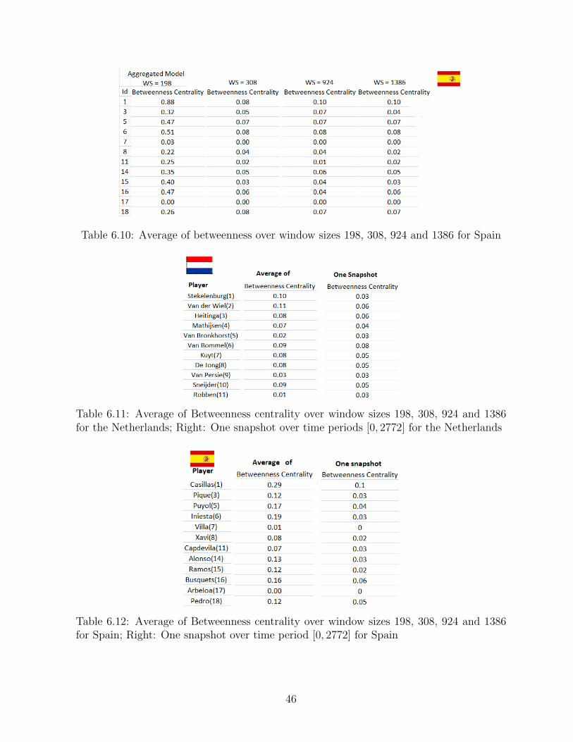
Table 6.10: Average of betweenness over window sizes 198, 308, 924 and 1386 for Spain

Table 6.11: Average of Betweenness centrality over window sizes 198, 308, 924 and 1386for the Netherlands; Right: One snapshot over time periods [0, 2772] for the Netherlands

Table 6.12: Average of Betweenness centrality over window sizes 198, 308, 924 and 1386for Spain; Right: One snapshot over time period [0, 2772] for Spain

46

A closer look at Tables 6.9 and 6.10 gives us an indication of how betweenness cen-

trality changes over different window sizes. We notice that betweenness centrality is not

increasing when window sizes are increasing. In fact, in both tables, there is a fluctuation

in betweenness centrality that can be caused by these changes. Table 6.12 shows that the

betweenness scores of most players in the single snapshot model is significantly smaller

than the average. When a player obtains the betweenness score in the single snapshot

network much bigger than in the aggregated model, such a player is getting good score

even in small window sizes. Therefore, he can be a good candidate to keep high score in

betweenness. For example, player number 1 (Casillas), not only is placed in the first rank

in aggregated model, but also the difference of his scores between the two models is very

high. On the other hand, he gets first rank in one snapshot model. The same phenomenon

occurs for the Netherlands; this is the case, for example, of player number 2 (Van der Wiel)

in Table 6.11

Some differences in the players’ rankings are noticeable between the static analysis and

the one based on aggregating windows. For example, the Spanish player number 8 (Pedro)

is ranked 6th by averaging the different size windows, while he is 3rd in the static analysis.

6.4 Pagerank in the Aggregated Model

In passing networks, the pagerank centrality of a player evaluates the probability that the

player will get the ball after a reasonable number of passes have been exchanged between

players in the team.

Tables 6.13 and 6.14 show that pagerank of each player for the two teams.

From Table 6.13 as we see, player number 1, the goalkeeper (Stekelenburg) has maxi-

mum pagerank score for each window sizes among all players in the Netherland team, and

from Table 6.14 we observe that two players: number 8 (Xavi) and number 18 (Pedro)

have maximum average pagerank scores among all players in the Spain team.

As we see, the average of pagerank for each players within a team over window sizes

is very close to the one that takes on one snapshot network and, in this case, we cannot

really observe any significant difference.

47

Table 6.13: Average of pagerank over window sizes 198, 308, 924 and 1386 for the Nether-lands

Table 6.14: Average of pagerank over window sizes 198, 308, 924 and 1386 for Spain

6.5 Clustering Coefficient in the Aggregated Model

The clustering coefficient gives us the degree to which players in a network tend to cluster to

each other. In our analysis we use clustering coefficient of each node (player) given in 3.22.

More precisely, for transitivity of the dynamic passing network we count the percentage

of all possible triangles consisting of the player. Suppose that player A wants to pass the

ball to player B, but since this line is blocked by a competitor he has to pass the ball to

C to reach player B. In this case, player A is acting as middle-man. For all other kind of

cycles, we are able to compute the clustering coefficient as explained in section 3.2.5.

48

Table 6.15: Average of Pagerank scores over window sizes 198, 308, 924 and 1386 for theNetherlands; Right: One snapshot over time period [0, 2772] for the Netherlands

Table 6.16: Average of Pagerank scores over window sizes 198, 308, 924 and 1386 for Spain;Right: One snapshot over time period [0, 2772] for Spain

In Table 6.17, we see that the clustering coefficient of most players is increasing with the

increase of the window sizes. Players number 6 and number 7 are the only players whose

measure is decreasing with the increase of the window size. In order to have a uniform

results for all players we need to take average over all window sizes, this would also give

49

Table 6.17: Average of Clustering coefficient over window sizes 198, 308, 924 and 1386 forthe Netherlands

more informative results. By taking average over all window sizes, we see that player

number 11 (Robben) has highest score equal to 0.56 among all players in the Netherlands

team.

Table 6.18: Average of clustering coefficient over window sizes 198, 308, 924 and 1386 forSpain

Table 6.18 shows the clustering coefficient of all players with different window sizes

within the Spain team. As we see, player number 7 (Villa) has the highest average clustering

coefficient score (0.47). In addition, Villa has maximum value of clustering coefficient in

each window size. This means that Villa has a largest balance between the amount of

passes involved in the team.

Table 6.19 shows that the maximum value of average clustering coefficient of players in

the Netherland team belongs to player number 11 (Robben). From the same table we see

that Robben has also maximum score in the single snapshot network.

As for the other parameters studied so far, there is generally not a big difference between

50

Table 6.19: Average of Clustering coefficient over window sizes 198, 308, 924 and 1386 forthe Netherlands; Right: One snapshot over time period [0, 2772] for the Netherlands

Table 6.20: Average of Clustering coefficient over window sizes 198, 308, 924 and 1386 forSpain; Right: One snapshot over time period [0, 2772] for Spain

the static analysis and the one based on aggregated windows, but some players are placed

in rather different ranks. This is the case, for example, of the Netherlands goalkeeper, who

is ranked 3rd in the static analysis, while he is ranked last with the aggregated windows

method.

51

6.6 Eigenvector Centrality in the Aggregated Model

The eigenvector centrality evaluates the most central players i.e. those with the smallest

“farness” from others, in terms of the global structure of the network. In fact, this score

pays less attention to patterns that are more local. As we explained in section 3.2.4, this

measure identifies dimensions of the distances among players. The location of each player

with respect to each dimension is called an eigenvalue, and the collection of such values is

called the eigenvector. Two highest eigenvector centralities in the Netherlands team are

Table 6.21: Average of eigenvector centrality over window sizes 198, 308, 924 and 1386 forthe Netherlands

player number 10 (Sneijder), and player number 8 (De Jong). This means that Sneijder

and Jong have smallest “farness” from others in the team, and their removal from the

match would have a great impact on the performance of the team. In the Spain team,

Table 6.22: Average of eigenvector centrality over window sizes 198, 308, 924 and 1386 forSpain

Table 6.22 shows that the two highest eigenvector centrality scores are for player number

52

18 (Pedro) and player number 14 (Alonso).

Another observation from Tables 6.22 and 6.21 is that a fluctuation in eigenvector

centralities occurs by increasing window sizes. In other words, there is no correlation

between eigenvector measures and the size of the windows. In order to get a stable result,

we take the average of eigenvector centrality of players over all window sizes and compare

them with eigenvector centrality captured from one snapshot, see Table 6.23 and 6.24.

Table 6.23: Average of Eigenvector centrality over window sizes 198, 308, 924 and 1386 forthe Netherlands; Right: One snapshot over time period [0, 2772] for the Netherlands

In Table 6.23 we see that the maximum eigenvector centrality captured by taking the

average of scores over the window sizes and in the single snapshot network, belong to player

number 10 (Sneijder) in the Netherlands. By the same observation from Table 6.24, we

see that player number 18 (Pedro) has the maximum score in both models. Also in this

case, however, the rankings of the players are not always preserved. Consider, for example,

player 11 (Capdevila) in the Spain team, who is ranked 9th in the aggregated windows

model, while is 6th in the static model.

6.7 Conclusions

In this chapter we studied degree centrality, closeness, betweenness, pagerank, and cluster-

ing coefficient in the the aggregated model. Below are some general conclusions we could

make.

From the fact that degree and pagerank of the Netherlands goalkeeper are the highest

among all the players, we infer that the ball is flowing around the Netherlands net, while

53

Table 6.24: Average of Eigenvector centrality over window sizes 198, 308, 924 and 1386 forSpain; Right: One snapshot over time period [0, 2772] for Spain

Spanish players keep it far from their net. The most important player in terms of degree

and pagerank is in fact the Netherlands goalkeeper.

The average of degree centrality of each players is increasing when the window size is

growing, that is, the degree centrality of each player in one snapshot network is greater than

the average over all window sizes. Therefore, the player with the highest degree centrality

within a team in one snapshot is also the one who has the highest degree by taking the

average of all degrees over the different window sizes in the team. A similar observation

holds also for closeness centrality.

We observed the fluctuation of the betweenness score in the two teams noticing that,

although the betweenness scores of Spain players are lower than the ones of the Netherlands

players, they are however more smoothly distributed, indicating that Spain has a well-

balanced performance technique.

We have seen that there is no correlation between clustering coefficients in different

window sizes. For some players, a small window size produce greater score than large

window size. By taking the average of the scores over the window sizes we obtain then a

more informative result than scores in the single snapshot network.

By using the window model, we easily see the presence of players that are substituted

during the game; this is the case, for example, of Spanish player number 17 (Arbeloa) who

just played for a small time period in the team from the start point. In the single snapshot

model, this fact would have been less evident.

54

Chapter 7

Dynamic Passing Networks in the

Non-Overlapping Model

In this chapter, we compute the same measures studied in the previous chapter based on the

non-overlapping model, by partitioning the total time period into equal consecutive time

windows. We remind that in the non-overlapping model we consider 4 different window

sizes: 2772, 1386, 396, 99 corresponding to a single time period of the total time of the

match (2772 sec.), 2 consecutive periods of 1386 sec. each, 7 consecutive periods of 396

sec. each, 28 consecutive periods of 99 sec. each.

7.1 Degree in the Non-Overlapping Model

In this section we consider degree centrality in the non-overlapping model. This data has

been shown in Table 7.1 and 7.2 for the Netherlands and Spain, respectively. As expected,

by decreasing the number of windows, the degree is increasing for each player within a

team.

In Table 7.1 player number 7 (Kuyt) has maximum degree score within a team for

window size equal to 99, whereas player number 1 (Stekelenburg) has maximum score

within a team when window sizes are equal to 396 and 693. Moreover, we observe that the

most active player in terms of getting and passing the ball around his co-teammate is the

goalkeeper, Stekelenburg in the Netherlands team.

Tables 7.3 and 7.4 show the values calculated for the single snapshot model and for

the average of the various windows in the non-overlapping windows model. No significant

difference can be observed in this case.

55

Table 7.1: Average of weighted degrees for window sizes 99, 396 and 693 for the Netherlands

Table 7.2: Average of weighted degrees for window sizes 99, 396 and 693 for Spain

Since player 17 has non zero degree value over [0, 396], it means that he is in the field.

However, his degree for the other windows vanishes. We conclude that he has been removed

from the game, observation that could not be done by inspection of the single snapshot

model. Another observation we can make from Graph 7.5 is that in different window times,

the number of passing between players in Spain is much higher than the one of players in

the Netherlands. This can be seen even better in Figure 7.5, where a window division has

been fixed and the variations of degrees can be observed in time for all players through

consecutive time intervals for a portion of the game.

56

Table 7.3: Average of degree centrality over window sizes 99, 396 and 693 for the Nether-lands; Right: One snapshot over time period [0, 2772] for the Netherlands

Table 7.4: Average of degree centrality over window sizes 99, 396 and 693 for Spain; Right:One snapshot over time period [0, 2772] for the Netherlands

7.2 Closeness in the Non-Overlapping Model

As explained in section 6.2, because of the character of passing network, closeness centrality

of a player must be computed by formula given in 3.12, where the length of a shortest path

between two nodes are given by formula 3.11.

Tables 7.6 and 7.7 show the closeness centrality of each player within the corresponding

57

Table 7.5: Degree centrality of players over 4 consecutive windows

teams. By looking at the tables, we see that when the window size is increasing some scores

are increasing while some scores are decreasing. Therefore, in order to find who is the best

player in terms of how he is close to other players in the team, we take the average of

closeness centrality over the window sizes and we determine the highest average score.

Table 7.6: Average of closeness for window sizes 99, 396 and 693 for the Netherlands

Table 7.7: Average of closeness for window sizes 99, 396 and 693 for Spain

58

Table 7.8: Average of closeness over window sizes 99, 396 and 693 for the Netherlands;Right: One snapshot over time period [0, 2772] for the Netherlands

In Table 7.8, the first column of scores shows that player number 6 (Van Bommel) has

maximum score in the average of window sizes. The second column of scores indicates that

Van Bommel has also a maximum score in one snapshot network.

Table 7.9: Average of closeness over window sizes 99, 396 and 693 for Spain; Right: Onesnapshot over time period [0, 2772] for Spain

A significant difference is shown in Table 7.9 where we can see that the highest average

closeness in the windows model for the Spain team belongs to player number 14 (Alonso),

whereas player number 16 (Busquets) has the maximum score in the single snapshot net-

work. Another difference can be seen in the relative rankings of player 18 (Pedro), who is

8th in the windows model, while is ranked only 5th with a single snapshot.

59

7.3 Betweenness in the Non-Overlapping Model

The computation of betweenness centrality is based on 3.13, since the network under study

is a directed weighted network.

From Table 7.10 one can see that the betweenness centrality of players are generally

increasing with the increase of the window sizes with two exceptions: player number 7

and 8. By this observation, we can deduce that the ball flow among players does not

rely on these two players, since their betweenness scores are not distributed very well in

different time periods. As we see by the same Table, Casillas has maximum betweenness

score between all players regardless of the window sizes. Therefore, this highest score dose

not measure how Casillas is well-connected, but rather how the ball flow among the other

players relays on Casillas. As we noticed before, if a player’s betweenness score vanishes,

which is the case of players number 8 (De Jong) in the Netherlands and players number

7 (Villa) and 17 (Arbeloa)in the Spain team, then a player is not getting involved in the

match and so his removal from the team would not have much impact.

If we look at Table 6.11, we notice several discrepancies between the players rankings

under the single snapshot and the non-overlapping window model. For example, player

number 8 (De Jong) has the minimum scores among all players in the window model,

but not in the static one. Another difference we observe with the single snapshot model,

concerns player number 6 (Vam Bommel) who has the highest score within the team in

the static model, but is ranked only 10th in our model, where it is instead (Stekelenburg)

the one with maximum score. This seems to imply that the goalkeeper in the Netherlands

team has a high impact on flowing the ball among players in the team, role that was less

visible in the single snapshot model and that we already observed also in the aggregated

model.

If we look at Table 7.12, we see a fluctuation of betweenness scores in different window

sizes. For instance, betweenness score of player number 1 (Casillas) the goalkeeper, vanishes

in window size 99. Moreover, if we compare two betweenness scores in the average and in

the single snapshot model, given in Table 6.12 we observe that player number 3 (Pique)

has the highest average betweenness centrality among all players. We can also see that

player number 7 (Villa) has maximum betweenness score among all players regardless of

the window sizes (in one snapshot network). On the on other hand, by looking at the

scores of Villa from Table 7.12 we can determine that the performance of Villa in specific

time periods does not show that he could hold a maximum score among the players in the

team. This is one important advantage of the non-overlapping slide window model that

60

Table 7.10: Average of Betweenness over window sizes 99, 396 and 693 for the Netherlands

can make clear the performance of players which can not be seen in the aggregated model.

As before, we notice that if a player’s betweenness score vanishes, which is the case of

players number 7 and 17 in the Spain team and player 11 in the Netherlands team, then

a player is not getting involved in the match and so his removal from the team would not

have much impact. e also note that the score of player number 17 (Arbeloa) vanishes as

well, but this player was playing only for a few minutes in the team. That is why we take

out his scores from our table.

By comparing betweenness centralities for players in two teams from Tables 7.11 and

7.12, we can conclude that there is more fluctuation in the Netherlands than in Spain,

meaning that the scores are more evenly distributed among the players in Spain. As

already observed in the analysis with the aggregated model, this may indicate that Spain

has a well-balanced performance technique.

An interesting observation is about player number 6 (Vam Bommel) who is placed at

first rank of betweenness scores in one snapshot network, but his score is second last in the

non-overlapping model. An explanation can be given also by observing a portion of the

match in time without averaging the window sizes. (see Figure 7.14) for the two teams.

The graph shows that Vam Bommel has a high score in interval [792, 1188], which however

becomes zero in the following interval [1188, 1980]. Having the highest score in one of the

intervals implies the maximum value in the single snapshot model.

61

Table 7.11: Average of betweenness centrality over window sizes 99, 396 and 693 for theNetherlands; Right: One snapshot over time periods [0, 2772] for the Netherlands

Table 7.12: Average of betweenness over window sizes 99, 396 and 693 for Spain

7.4 Pagerank in the Non-Overlapping Model

As mentioned in Section 6.4, roughly speaking, the pagerank centrality of a player in

passing networks gives the probability that he will get the ball after a reasonable number

of passes have been done between players in the team. The computation of pagerank score

in our model is based on formula 3.19 described in section 6.4.

As we see from Tables 7.15 and 7.16, in both teams the scores are for the most part

decreasing with the increase of the window size. This means that in most of the cases,

a player gets smaller pagerank than he is expected to get over a large window size. By

62

Table 7.13: Average of betweenness centrality over window sizes 99, 396 and 693 for Spain;Right: One snapshot over time period [0, 2772] for Spain

Table 7.14: Betweenness centrality of players in 4 consecutive windows

Table 7.15: Average of pagerank over window sizes 99, 396 and 693 for the Netherlands

taking the average over all window sizes, we will obtain small score compared with taking

the average of scores over small window sizes.

63

Table 7.16: Average of pagerank over window sizes 99, 396 and 693 for Spain

Table 7.17: Average of pagerank centrality over window sizes 99, 396 and 693 for Spain;Right: One snapshot over time period [0, 2772] for Spain

We conclude that the most important players in the Spain team seem to be players num-

ber 8 (Xavi) and number 18 (Pedro), while player number 1 (Stekelenburg) the goalkeeper

is most important player in the Netherlands.

We notice that in terms of pagerank score, the performance of Spain is higher than the

one of Netherlands. The reason is twofold: on one hand, the fact that the pagerank score

of the goalkeeper is high implies that Spain players keep the ball near to the Netherlands

net, or shoot the ball into the Netherlands net. Second, the fluctuation of pagerank scores

64

Table 7.18: Average of pagerank centrality over window sizes 99, 396 and 693 for theNetherlands; Right: One snapshot over time period [0, 2772] for the Netherlands

in Spain is much lower than the fluctuation for the Netherlands. This is again an indication

of the defensive nature of the Netherlans’ play versus the more aggressive play of Spain.

This behaviour is evident also by inspecting the variations of pagerank for a portion of

the game, and for a given window size (see Figure 7.19).

Table 7.19: Pagerank score of players for 4 consecutive windows

7.5 Clustering Coefficient in the Non-Overlapping Model

The clustering coefficient is calculated by the formula given in 3.22. As we saw in section

3.2.5, there are four models of directed triangles consisting a fix node, In, Out, Cycle and

Middle-man. For each player, as a node of the network, we count the percentage of all

possible triangles consisting of the node.

65

Table 7.20: Average of Clustering coefficient over window sizes 99, 396 and 693 for theNetherlands

Table 7.21: Average of clustering coefficient over window sizes 99, 396 and 693 for Spain

Tables 7.20 and 7.21 shows the clustering coefficient of players in each team is increasing

by growing the window sizes.

From Tables 7.22 and 7.23, we find that player number 7 (Kuyt) in the Netherlands

team and player number 3 (Pique) in the Spain team have highest average scores among

the players of their own team. Whereas player number 11 (Robben) in the Netherlands

and player number 7 (Villa) in Spain have the highest score.

By inspecting Tables 7.20 and 7.21 we notice that Stekelemburg, the Netherlands goal-

keeper has the same anomalous behaviour already remarked in the aggregated window

model: he is ranked 3rd in the static analysis, while he is ranked much lower int the

66

Table 7.22: Average of Clustering coefficient over window sizes 99, 396 and 693 for theNetherlands; Right: One snapshot over time period [0, 2772] for the Netherlands

Table 7.23: Average of Clustering coefficient over window sizes 99, 396 and 693 for Spain;Right: One snapshot over time period [0, 2772] for Spain

windows method.

Another interesting observation regards player number 5 (Van Bronkhorst) in the

Netherlands team, who appears to be one of best players within the team, with a large

balance in the amount of passes. In fact, his score is increasing smoothly from window size

99 to window size 693 with a very small difference among the clustering coefficients within

the various window sizes. This small fluctuation indicates that Bronkhorst has kept a

constant high level performance during the match. Note that such an observation emerges

from the non-overlapping model, but could not be seen in the single snapshot network.

67

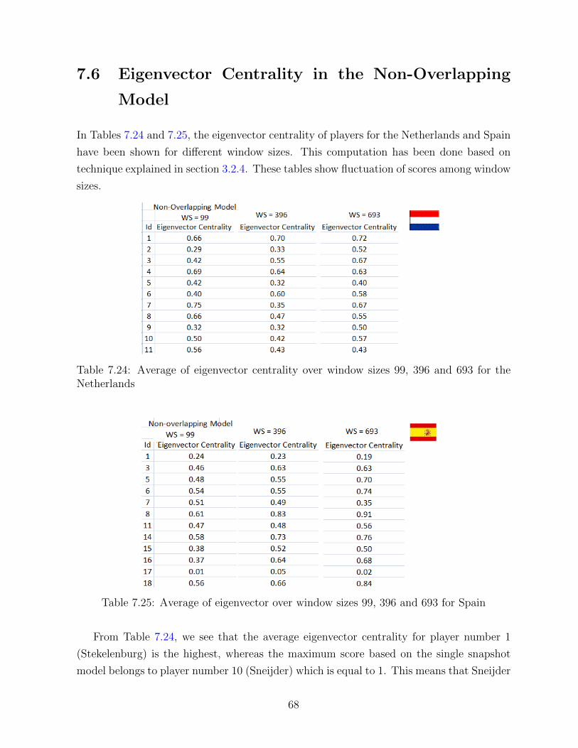
7.6 Eigenvector Centrality in the Non-Overlapping

Model

In Tables 7.24 and 7.25, the eigenvector centrality of players for the Netherlands and Spain

have been shown for different window sizes. This computation has been done based on

technique explained in section 3.2.4. These tables show fluctuation of scores among window

sizes.

Table 7.24: Average of eigenvector centrality over window sizes 99, 396 and 693 for theNetherlands

Table 7.25: Average of eigenvector over window sizes 99, 396 and 693 for Spain

From Table 7.24, we see that the average eigenvector centrality for player number 1

(Stekelenburg) is the highest, whereas the maximum score based on the single snapshot

model belongs to player number 10 (Sneijder) which is equal to 1. This means that Sneijder

68

has smallest “farness” from the others in the single snapshot network, whereas he has no

high score if we look at his activity over different time periods, where he is actually ranked

quite low. The same phenomenon occurs in the Spain team, where player number 8 (Xavi)

has the maximum average score, whereas in the single snapshot model player number 18

(Pedro) has the maximum score (see Table 7.27). Again, if we focus on Pedro’s scores in

different window sizes, we see that he is not obtaining maximum score in each window sizes

(Table 7.25) indicating an uneven performance.

Table 7.26: Average of eigenvector centrality over window sizes 99, 396 and 693 for theNetherlands; Right: One snapshot over time period [0, 2772] for the Netherlands

Table 7.27: Average of eigenvector centrality over window sizes 99, 396 and 693 for Spain;Right: One snapshot over time period [0, 2772] for Spain

69

7.7 Conclusions

In this chapter, we studied degree centrality, closeness, betweenness, pagerank, and cluster-

ing coefficient in the the non-overlapping window model. Below are some general conclu-

sions we could make, most confirming what already observed with the aggregated model.

We have noticed that the most important players in the Spain team seem to be play-

ers number 8 (Xavi) and number 18 (Pedro), while player number 1 (Stekelenburg), the

goalkeeper, being the most important player in the Netherlands.

We have seen that in terms of pagerank score, the performance of Spain is higher than

the one of Netherlands. Indeed, since the pagerank score of the goalkeeper is high, we

conclude that Spain players keep the ball near to the Netherlands net, or shoot the ball

into the Netherlands net. Moreover, we observed that, the fluctuation of pagerank scores

in Spain is much lower than the fluctuation for the Netherlands. This is again an indication

of the defensive nature of the Netherlans’ play versus the more aggressive play of Spain.

Another consequence of our case study concerns player number 5 (Van Bronkhorst)

in the Netherlands team, who appears to be one of best players within the team, with

a large balance in the amount of passes. We have seen that his score (degree centrality)

is increasing evenly from window size 99 to window size 693 with a very small difference

among the clustering coefficients within the various window sizes.

Different results have been captured using non-overlapping model in comparison with

the static analysis; for example, by this, possibly more accurate, analysis, we see that

the highest closeness score belongs to player number 14 (Alonso), whereas in the single

snapshot model the maximum closeness is taken by player number 16 (Busquets).

Finally, player number 17 (Arbeloa) in the Spain team has extremely low scores of

degree, betweenness and closeness over different widow size, as well as in the single snap-

shot model. From the non-overlapping window times, we can deduce that he has been

substituted very soon after the start of the game.

70

Chapter 8

Conclusions

In the current literature, football passing networks have been analyzed on the basis of

static representations of football matches. In the thesis we propose to include temporal

information in the match description and to take advantage of it to obtain possibly more

accurate information about the weaknesses, strengths and connections among the players,

and about the general behaviours of the team.

To do so, we adapted to our setting the centrality measures previously studied in the

context of football passing networks: degree centrality, closeness, betweenness, pagerank,

clustering coefficient and eigenvector centrality. These measures have been studied for

static football passing networks representations, while we investigated them in two tempo-

ral models: one where time is partitioned in consecutive periods (non-overlapping windows)

and another where the global play time is observed in growing time intervals (aggregated

windows). The observations of those centrality parameters in the windows models has al-

lowed us to detect interesting information about the players and about the teams, several

of which could not be detected by the inspection of the static representation of the passing

network.

To the best of our knowledge this is the first time that a football match has been studied

focusing on the passes among players in time, and the results of the thesis constitutes a

very first step towards a more complete analysis. The techniques and results of the thesis,

in fact, contain several limitations and they open more problems than they close. For

example:

• Some temporal measures based on the dynamic nature of the time varying graph

that represents the football passing network could be employed. This is the case, for

example, of foremost and fastest betweenness, where the “static” notion of shortest

71

path is substituted by the temporal notions of “fastest” or “earliest” path. The inves-

tigation of such measures could bring a totally different perspective to the temporal

study of football matches.

• Different types of windows could be considered; for example, another option would

be to perform the analysis with overlapping windows where the corresponding time

intervals overlap of variable amounts.

• A study that should be performed is to focus on individual players and analyze

their scores in time, after fixing a certain window size. This study would allow the

analysis of the scores fluctuations in time and would identify specific characteristics

of the players behaviour during the match. For lack of time, we observed only partial

data in this fashion (e.g., see Figures 7.1) but a full analysis is left for future study.

• Another very interesting direction would be the study of passing patterns of successful

teams, so to learn information about play strategies, and to understand patterns

associated to weak or strong players.

• A study that could be of interest is to incorporate the information about shots to-

wards the opposite goalkeeper and use social networks tools to analyze the resulting

network.

• Finally, techniques similar to the ones of the thesis could be employed to focus on

successful and incomplete passes within players in a team.

72

References

[1] A. Balasubramanian, Y. Zhou, W. B. Croft, B. N. Levine, and A. Venkataramani.

Web search from a bus. In Proceedings of the 2nd workshop on Challenged networks

CHANTS - CHANTS ’07, page 59-66, 2007.

[2] M. Bastian, S. Heymann, and M. Jacomy. Gephi: An open source software for explor-

ing and manipulating networks. In Proceedings of 3rd International AAAI Conference

on Weblogs and Social Media, pages 361–362, 2009.

[3] P. Bonacich. Power and centrality: A family of measures. American journal of soci-

ology, pages 1170–1182, 1987.

[4] S. P. Borgatti. Centrality and network flow. Social Networks, 27(1):55–71, 2005.

[5] S. P. Borgatti and M. G. Everett. A graph-theoretic perspective on centrality. Social

networks, 28(4):466–484, 2006.

[6] J. Burgess, B. Gallagher, D. Jensen, and B. N. Levine. MaxProp: Routing for Vehicle-

Based Disruption-Tolerant Networks. In INFOCOM, volume 6, pages 1–11, 2006.

[7] R. S. Burt. Structural holes: The social structure of competition, volume 58. 1992.

[8] A. Casteigts, P. Flocchini, W. Quattrociocchi, and N. Santoro. Time-varying graphs

and dynamic networks. International Journal of Parallel, Emergent and Distributed

Systems, 27(5): 387-408, 2012.

[9] Augustin Chaintreau, Pan Hui, Jon Crowcroft, Christophe Diot, Richard Gass, and

James Scott. Impact of human mobility on opportunistic forwarding algorithms. IEEE

Transactions on Mobile Computing, 6(6):606–620, 2007.

[10] E. W. Dijkstra. A note on two problems in connexion with graphs. Numerische

Mathematik, 1(1):269–271, 1959.

73

[11] G. Fagiolo. Clustering in complex directed networks. Physical Review E - Statistical,

Nonlinear, and Soft Matter Physics, 76(2), 2007.

[12] A. Ferreira. Building a reference combinatorial model for MANETs. Networks,

18(5):24–29, 2004.

[13] P. Flocchini, B. Mans, and N. Santoro. On the exploration of time-varying networks

In Theoretical Computer Science 469: 53-68, 2013.

[14] I. Franks and M. Hughes. Analysis of passing sequences, shots and goals in soccer. J.

Sports Sci., 5(23):509–514, 2005.

[15] L. C. Freeman. Centrality in social networks conceptual clarification, Social Networks,

1(3):215-239, 1978. 1978.

[16] L. C. Freeman. The development of social network analysis: A study in the sociology

of science, BookSurge, 2004.

[17] H. Gerth and K. Wolff. The sociology of Seorg Simmel, The Free Press, 1950.

[18] C. Godsil. Algebraic combinatorics, CRC Press, 1993.

[19] P. Gould. On the geographical interpretation of eigenvalues. Transactions of the

Institute of British Geographers, pages 53–86, 1967.

[20] J. Gudmundsson and T. Wolle. Football analysis using spatio-temporal tools. Com-

puters, Environment and Urban Systems, pages 16–27.

[21] P. Jacquet, B. Mans, and G. Rodolakis. Information propagation speed in mobile and

delay tolerant networks. IEEE Transactions on Information Theory, 56(10):5001–

5015, 2010.

[22] K. Jain, J. Padhye, V. N. Padmanabhan, and L. Qiu. Impact of iterference on multi-

hop wireless network performance. Wireless Networks, 11(4):471–487, 2005.

[23] C. H. Kang, J. R. Hwang, and K. J. Li. Trajectory analysis for soccer players. In

Proceedings 6th IEEE International Conference on Data Mining, pages 377–38, 2006.

[24] L. Katz. A new status index derived from sociometric analysis. Psychometrika,

18(1):39–43, 1953.

74

[25] D. Kempe, J. Kleinberg, and A. Kumar. Connectivity and inference problems for

temporal networks. In Proceedings of the 32nd annual ACM symposium on Theory of

computing - STOC ’00, pages 504–513, 2000.

[26] D. Kempe, J. Kleinberg, and E. Tardos. Maximizing the spread of influence through

a social network. Proceedings of the 9th ACM SIGKDD international conference on

Knowledge discovery and data mining - KDD ’03, page 137, 2003.

[27] H. C. Kim, O. Kwon, and K. J. Li. Spatial and spatiotemporal analysis of soccer. In

Proceedings of the 19th ACM SIGSPATIAL International Conference on Advances in

Geographic Information Systems, pages 385–388. ACM, 2011.

[28] J. Leskovec, L. A Adamic, and B. A. Huberman. The dynamics of viral marketing.

ACM Transactions on the Web, 1(1):5, 2007.

[29] J. Leskovec, J. Kleinberg, and C. Faloutsos. Graph evolution: Densification and

shrinking diameters. ACM Transactions on Knowledge Discovery from Data (TKDD),

1(1):2, 2007.

[30] J. B. Linde and M. Lø kketangen. Predicting outcomes of association football

matches based on individual players’ performance. Master thesis, Norges teknisk-

naturvitenskapelige universitet, http://hdl.handle.net/11250/253820, 2014.

[31] Cong Liu and Jie Wu. Scalable routing in cyclic mobile networks. IEEE Transactions

on Parallel and Distributed Systems, 20(9):1325–1338, 2009.

[32] M. McPherson, L. Smith-Lovin, and J. M. Cook. Birds of a feather: Homophily in

social networks, Annual Review of Sociology, 27: 415-444, 2001.

[33] M. Newman. Networks: an introduction. Oxford University Press, 2010.

[34] M. E. J. Newman. Scientific collaboration networks. II. Shortest paths, weighted

networks, and centrality. Physical review E, 64(1 Pt 2):16132, 2001.

[35] M. E J Newman. Analysis of weighted networks. Physical Review E - Statistical,

Nonlinear, and Soft Matter Physics, 70(5), 2004.

[36] T. Opsahl, F. Agneessens, and J. Skvoretz. Node centrality in weighted networks:

Generalizing degree and shortest paths. Social Networks, 32(3):245–251, 2010.

[37] T. Opsahl, V. Colizza, P. Panzarasa, and J. J. Ramasco. Prominence and control:

The weighted rich-club effect. Physical Review Letters, 101(16), 2008.

75

[38] L. Page, S. Brin, R. Motwani, and T. Winograd. The PageRank citation rank-

ing:bringing order to the web., Technical Report, Stanford InfoLab, 1999.

[39] J. L. Pena and H. Touchette. A network theory analysis of football strategies. arXiv

preprint arXiv:1206.6904, 2012.

[40] E. R. Peay. Connectedness in a general model for valued networks, Social Networks,

2(4): 385410, 1980.

[41] Z. Qianwei. Analysis on the connotation of passing in football matches. Journal of

Chengdu Physical Education Institute, volume 6, 2003.

[42] P. Ruiz, B. Dorronsoro, P. Bouvry, and L. Tardon. Information dissemination in

VANETs based upon a tree topology. Ad Hoc Networks, 10(1):111–127, 2012.

[43] T. Spyropoulos, K. Psounis, and C. S. Raghavendra. Spray and wait. In Proceeding

of the 2005 ACM SIGCOMM workshop on Delay-tolerant networking - WDTN ’05,

pages 252–259, 2005.

[44] A. Tucker. Applied combinatorics, 1984.

[45] S. Wasserman and K. Faust. Social network analysis: Methods and applications.

Cambridge University Press, 1993.

[46] D. J. Watts and S. H. Strogatz. Collective dynamics of ’small-world’ networks. Nature,

393(6684):440–442, 1998.

[47] W. Xing and A. Ghorbani. Weighted pagerank algorithm. In Proceedings of the 2nd

Annual Conference on Communication Networks and Services Research, 305 - 314,

2004.

[48] S. Yang and D. Knoke. Optimal connections: Strength and distance in valued graphs.

Social Networks, 23(4):285–295, 2001.

[49] D. Zhang, S. A. Gogi, D. S. Broyles, E. K. Cetinkaya, and J. P. G. Sterbenz. Modelling

wireless challenges. In Proceedings of the 18th annual international conference on

Mobile computing and networking - Mobicom ’12, page 423-426, 2012.

[50] X. Zhang, J. K. Kurose, B. N. Levine, D. Towsley, and H. Zhang. Study of a bus-based

disruption-tolerant network: mobility modeling and impact on routing. In Proceedings

of the 13th annual ACM international conference on Mobile computing and networking

- MobiCom ’07, pages 195-206, 2007.

76