analytical solution of option pricing for two stocks by
TRANSCRIPT

Analytical solution of option pricing for two Stocks by time fractional
ordered Black Scholes partial differential equation
Dr. Kamran Zakaria, Muhammad Saeed Hafeez
Department of Mathematics, NED University of Engineering and Technology, Karachi
Abstract
Time fractional order Black scholes partial differential equation for risk free
option pricing in financial market yields the better prediction in financial market of
the country. In this paper the modified form of Black Schole equation including
two stocks is used for evaluations. Samudu Transform approach is utilized for
calculating analytical solution . Solution of the equation has been found in form
of convergent infinite series.
Keywords:
Options, Samudu Transforms, Caputo Derivative, the time fractional order partial differential
equation, Black Scholes Equation.
Introduction:
This paper is the extended version of the paper presented in 3rd International
Conference on Computing, Mathematics and Engineering Technologies (iCoMET)
2020 as given in the reference [1].
Option pricing is the worldwide growing field of financial mathematics to solve
financial market pricing problems. It is a not very old discipline consists of
techniques to predict the prices of assets in financial market. The Black Scholes

mathematical model with aid of computer science provides the tool to solve
complex financial markets, stock exchange and industrial problems. under
discussion model is the benchmark imitations in finance, and it is the first
mathematical models which predicts the pricing of options (both call and put) and
the implied volatility.
The Maximum payoff is always the wish of successful businessman and it is
possible only when the risk is minimized and gain is maximized. Specifically, the
stock exchange is the good example for option pricing where the prices of shares
are highly uncertain and unpredictable. But the risk free prices may be obtained by
using the famous Black Scholes partial differential equation.
Price and share option valuation of options have been a comer stone in financial
markets. Financial study of financial derivatives is one of two most growing areas
in the corporate business finance . The mathematical models are servings to
measure the variation, predict and forecast the behavior of financial markets.
The Fractional calculus presents a highly endorsement and latest tool in business
finance. Time fractional ordered Business Financial models are expressed in form
fractional ordered stochastic PDE to maintain better accuracy and tolerance, to
control variations and investigate random -ness in financial markets.
Black-Scholes model is the prominent and well known models to evaluate the
option prices containing the brief literature review of its empirical developments
theme of beginning with Black and Scholes (1973) experimental examinations
close predisposition inside the Black-Scholes model as far as moneyness and
development.
Studies have been growing additionally noted instability inclination operating at a
profit Black Scholes model (1973) utilizing S&P 500 choice list information 1966-
1969 recommend the fluctuation that appertain the choice delivers a cost among
the framework’s cost and market cost. Black and Scholes (1973) propose proof,
instability isn't fixed. Galai (1977) affirm B-S model that the supposition of
verifiable momentary instability need to be loose. Their observational outcomes
are likewise steady with the consequences of Geske in the year 1979.MacBeth and
Merville (1980) look at the Black-Scholes model against the steady flexibility of
difference (CEV) model, which expect unpredictability changes when the stock
costs changes. MacBeth and Merville (1980) found that the unpredictability of the
hidden stock minimized the risk as the stock value rises.
Beckers (1980) tried the Black-Scholes suspicion that the chronicled quick
unpredictability of the fundamental stock is a component of the stock value,
utilizing S&P 500 record alternatives 1972-1977. Beckers (1980) finds the hidden
stock is a converse capacity of the stock cost.
Geske and Roll (1984) show that at a unique time both in-the-cash and out-of-the-
cash choices contain instability inclination. Geske and Roll (1984) finish up, time
and cash predisposition might be identified with inappropriate limit conditions,
where as the unpredictability inclination issue might be the consequence of
measurable mistakes in estimation.
Rubinstein (1994) shows that the inferred instability for S&P 500 file choices
applies abundance kurtosis. Shimko (1993) exhibits that inferred conveyances of
S&P 500 record are contrarily slanted and leptokurtic. Jackwerth and Rubinstein
(1996) show the dispersion of the S&P 500 preceding 1987 apply lognormal
appropriations, however since have disintegrated to look like leptokurtosis and
negative skewness. A few examinations try to expand the tail properties of the
lognormal conveyance by consolidating a hop dissemination process or stochastic
instability.
Das and Sundaram (1999) show hop dispersion and stochastic instability moderate
yet don't take out unpredictability predisposition. Das and Sundaram (1999)
recognize hop dispersion and stochastic instability forms don't produce skewness
and extra kurtosis looked like actually.
Buraschi and Jackwerth (2001) create measurable tests dependent on prompt
model and stochastic models utilizing S&P 500 list alternatives information from
1986-1995. Buraschi and Jackwerth (2001) close the information is progressively
steady with models that contain extra hazard factors, for example, stochastic
unpredictability and hop dissemination.
Yang (2006) finds suggested volatilities used to esteem trade exchanged call
alternatives on the ASX 200 Index are fair-minded and better than chronicled
immediate unpredictability in guaging future acknowledged instability. Yang
(2006) finds inferred volatilities used to esteem trade exchanged call alternatives
on the ASX 2000 Index are fair and better than authentic immediate instability in
determining future acknowledged unpredictability. Writing proposes the Black-
Scholes model may undervalue alternatives in light of the fact that the tail
properties of the hidden lognormal dissemination are excessively little.
In 2016, H. Zhang, F. Liu I. Turner, Q. Yang solved time fractional
Black–Scholes model governing equation for European options numerically.
In 2019, D. Prathumwan and K. Trachoo solved Black Sholes equation

by the method of Laplace Homotopy Perturbation Method for two asset
option pricing [1].
In this paper, the technique of Samudu transform method is used to
demonstrate the analytical solution of 2-Dimensional, Time Fractional-ordered
BS-Model, consists of two different assets in Liouville- Caputo Fractional
derivative form for the European call options. The Sammudu Transform
provides the value of put option in form of explicit solution in convergent
series. In Lapace perturbation method, first step the method of Laplace
transform is applied then homotopy method is applied. The solution is
found by the certain hectic work but in the method of Samudu Transform, the
solution may be found without such a hectic working. The solution is similar
to the solution obtained by the method of Laplace Homotopy method.
The method for solving two assets BS financial model is described in
next section.
Methodology
Consider P.D.E.
𝜕∝
𝜕𝑡∝ ∅ 𝑥, 𝑦, 𝑡 + ⎿∅ 𝑥, 𝑦, 𝑡 + 𝑁∅ 𝑥, 𝑦, 𝑡 = 𝑓 𝑥, 𝑦, 𝑡 − − − − − − − (𝑖)
Where 𝑛 − 1 <∝≤ 𝑛; 𝑛 ∈ 𝑁
Subject to:
∅ 𝑥, 𝑦, 0 = ∅0 (𝑥, 𝑦)
Where 𝐿 = Linear Differential operator
𝑁 = Non -Linear Differential operator

Call Sumudu Transform for the caputo Fractional ordered Derivative of ∅ 𝑥, 𝑦, 𝑡 on because of
equation (i)
𝑆 𝜕∝
𝜕𝑡∝ ∅ 𝑥, 𝑦, 𝑡 = 𝑠[ ∅ 𝑥, 𝑦, 𝑡 − ⎿∅ 𝑥, 𝑦, 𝑡 − 𝑁∅ 𝑥, 𝑦, 𝑡 + 𝑓 𝑥, 𝑦, 𝑡 − − − − − − − (𝑖𝑖)
𝑆 𝜕∝
𝜕𝑡∝ ∅ 𝑥, 𝑦, 𝑡 = 𝑢−∝𝑠[∅ 𝑥, 𝑦, 𝑡 − 𝑢−∝+𝑘
𝑛−1
𝑘=0
𝜕𝑘
𝜕𝑡𝑘 ∅(𝑥, 𝑦, 0)
If ∝< 1, setting 𝑛 = 1
𝑆 𝜕∝
𝜕𝑡∝ ∅ 𝑥, 𝑦, 𝑡 = 𝑢−∝𝑠 ∅ 𝑥, 𝑦, 𝑡 − 𝑢−∝ ∅ 𝑥, 𝑦, 0
𝑢−∝𝑠 ∅ 𝑥, 𝑦, 𝑡 − 𝑢−∝ ∅ 𝑥, 𝑦, 0 = 𝑠 [𝑓 𝑥, 𝑦, 𝑡 − ⎿ ∅ 𝑥, 𝑦, 𝑡 − 𝑁∅ 𝑥, 𝑦, 𝑡
𝑠 ∅ 𝑥, 𝑦, 𝑡 = ∅ 𝑥, 𝑦, 0 + 𝑢−∝𝑠 [𝑓 𝑥, 𝑦, 𝑡 − ⎿ ∅ 𝑥, 𝑦, 𝑡 − 𝑁∅ 𝑥, 𝑦, 𝑡
Apply Inverse Sumudu Transform.
𝑠 𝑠−1∅ 𝑥, 𝑦, 𝑡 = 𝑠−1 ∅ 𝑥, 𝑦, 0 + 𝑠−1 𝑢∝𝑠 𝑓 𝑥, 𝑦, 𝑡 − ⎿ ∅ 𝑥, 𝑦, 𝑡 − 𝑁∅ 𝑥, 𝑦, 𝑡
Call Inverse property of Samudu Transform (S.T)
𝐼∝ 𝑔 𝑥, 𝑦, 𝑡 = 𝑠−1[𝑢∝𝑠(𝑔 𝑥, 𝑦, 𝑡 ]
Apply Integral Property of S.T on equation (3)
∅ 𝑥, 𝑦, 𝑡 = ∅0 𝑥, 𝑦 + 𝐼∝ [𝑓 𝑥, 𝑦, 𝑡 − ⎿ ∅ 𝑥, 𝑦, 𝑡 − 𝑁∅ 𝑥, 𝑦, 𝑡 − − − − − (4)
Sumudu Transform Express the so𝑙𝑛 of P.D.E in form of Infinite Convergent series
as below. (1)
∅ 𝑥, 𝑦, 𝑡 = ∅0 𝑥, 𝑦 + 𝑔𝑛(𝑥, 𝑦)𝑡𝑛∝
Γ(1 + 𝑛 ∝)
∞
𝑛=1
Where
∅0 𝑥, 𝑦 = 𝑔0 𝑥, 𝑦 = 𝑔0

𝑔1 = 𝑓 𝑥, 𝑦, 𝑡 − ⎿ 𝑔0 − 𝑁(𝑔0)]
𝑔2 = 𝑓 𝑥, 𝑦, 𝑡 − ⎿ 𝑔1 − 𝑁(𝑔1)]
𝑔3 = 𝑓 𝑥, 𝑦, 𝑡 − ⎿ 𝑔2 − 𝑁(𝑔2)]
⋮ ⋮
𝑔𝑛 = 𝑓 𝑥, 𝑦, 𝑡 − ⎿ 𝑔(𝑛) − 𝑁[𝑔(𝑛)]
This rearch paper is the application of Sumudu Integral Transform to evaluate option price of
two stocks Fractional order Black Sholes Model.
Consider below Fractional order European call option pricing P.D.E for two stocks.
𝜕∝𝑐
𝜕𝑡∝+
𝜎12
2𝑠1
2 𝜕2𝑐
𝜕𝑠12 +
𝜎22
2𝑠2
2 𝜕2𝑐
𝜕𝑠22 + 𝑟𝑠1
𝜕𝑐
𝜕𝑠1+ 𝑟𝑠1
𝜕𝑐
𝜕𝑠1+ 𝑟𝑠2
𝜕𝑐
𝜕𝑠2+ 𝑝 𝑠1𝑠1𝜎1𝜎2
𝜕2𝑐
𝜕𝑠1𝜕𝑠2− 𝑟𝑐 = 0
Subject to pay-off to the investor.
𝑐(𝑠1, 𝑠2 ,𝑡) = max (𝑤1 𝑠1 + 𝑤𝑠2 − 𝑘 , 0) ( for European Call Option)
P(𝑠1, 𝑠2 ,𝑡) = max (𝑤1 𝑠1 + 𝑤𝑠2 − 𝑘 , 0) ( for American Put option)
Where
c = value of European Call Option
P = value of American Call Option
𝑠1 = Price of share of stock 1
𝑠2 = Price of share of stock 2
P= correlation coefficient between price of shares of stock 1 and stock 2
𝜎1= Price volatility or S.D of stock 1

𝜎2= Price volatility or S.D of stock 2
K = Strike price or Exercise price for call option
𝑤1= properties of investment on stock 1
𝑤2= properties of investment on stock 2
Equation (4) can be simplified by considering the substitution.
𝑢 = 𝑙𝑛𝑠1 − 𝑟 − 1
2𝜎1
2 𝑡
𝑢 = 𝑙𝑛𝑠2 − 𝑟 − 1
2𝜎2
2 𝑡
𝜕𝑐
𝜕𝑠1=
𝜕𝑐
𝜕𝑢 𝜕𝑢
𝜕𝑠1
𝜕𝑐
𝜕𝑠2=
𝜕𝑐
𝜕𝑣 𝜕𝑢
𝜕𝑠2c
𝜕2𝑐
𝜕𝑠12 =
𝜕
𝜕𝑠1
𝜕𝑐
𝜕𝑢
=1
𝑠1=
𝜕
𝜕𝑠1
𝜕𝑐
𝜕𝑢 +
𝜕𝑐
𝜕𝑢
𝜕
𝜕𝑠1
1
𝑠1
=1
𝑠1=
𝜕
𝜕𝑢 𝜕𝑐
𝜕𝑢
𝜕𝑢
𝜕𝑠1− 𝑠1
2 𝜕𝑐
𝜕𝑢
=1
𝑠12
𝜕2𝑐
𝜕𝑢2−
1
𝑠2 𝜕𝑐
𝜕𝑢
𝜕𝑐
𝜕𝑠2=
1
𝑠2 𝜕𝑐
𝜕𝑣… . . . . . (2) 1 ………
𝜕𝑐
𝜕𝑠1=
1
𝑠1 𝜕𝑐
𝜕𝑢
𝑖𝑖 − − − − − −𝜕2𝑐
𝜕𝑠12 =
1
𝑠12 −
𝜕2𝑐
𝜕𝑢2−
𝜕𝑐
𝜕𝑢
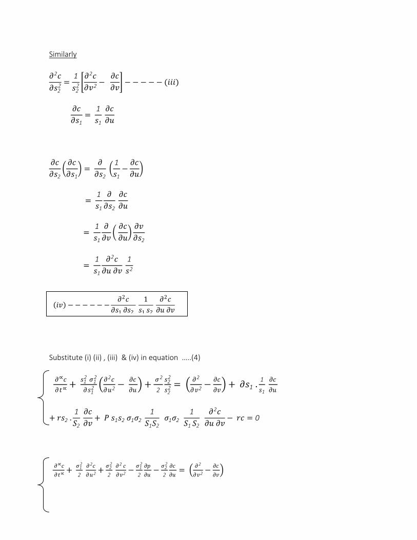
Similarly
𝜕2𝑐
𝜕𝑠22 =
1
𝑠22
𝜕2𝑐
𝜕𝑣2−
𝜕𝑐
𝜕𝑣 − − − − − (𝑖𝑖𝑖)
𝜕𝑐
𝜕𝑠1=
1
𝑠1 𝜕𝑐
𝜕𝑢
𝜕𝑐
𝜕𝑠2 𝜕𝑐
𝜕𝑠1 =
𝜕
𝜕𝑠2
1
𝑠1−
𝜕𝑐
𝜕𝑢
= 1
𝑠1
𝜕
𝜕𝑠2 𝜕𝑐
𝜕𝑢
= 1
𝑠1
𝜕
𝜕𝑣 𝜕𝑐
𝜕𝑢
𝜕𝑣
𝜕𝑠2
= 1
𝑠1
𝜕2𝑐
𝜕𝑢 𝜕𝑣
1
𝑠2
Substitute (i) (ii) , (iii) & (iv) in equation …..(4)
𝜕∝𝑐
𝜕𝑡∝+
𝑠1 2 𝜎1
2
𝜕𝑠12
𝜕2𝑐
𝜕𝑢2−
𝜕𝑐
𝜕𝑢 +
𝜎2
2
𝑠22
𝑠22 =
𝜕2
𝜕𝑣2−
𝜕𝑐
𝜕𝑣 + 𝜕𝑠1 .
1
𝑠1 𝜕𝑐
𝜕𝑢
+ 𝑟𝑠2 .1
𝑆2 𝜕𝑐
𝜕𝑣+ 𝑃 𝑠1𝑠2 𝜎1𝜎2
1
𝑆1𝑆2 𝜎1𝜎2
1
𝑆1 𝑆2
𝜕2𝑐
𝜕𝑢 𝜕𝑣− 𝑟𝑐 = 0
𝜕∝𝑐
𝜕𝑡∝ + 𝜎1
2
2 𝜕2𝑐
𝜕𝑢2 +𝜎2
2
2 𝜕2 𝑐
𝜕𝑣2 −𝜎1
2
2
𝜕𝑝
𝜕𝑢−
𝜎22
2
𝜕𝑐
𝜕𝑢=
𝜕2
𝜕𝑣2 −𝜕𝑐
𝜕𝑣
𝑖𝑣 − − − − − −𝜕2𝑐
𝜕𝑠1 𝜕𝑠2
1
𝑠1 𝑠2
𝜕2𝑐
𝜕𝑢 𝜕𝑣
=1
𝑠12 −
𝜕2𝑝
𝜕𝑢2−
𝜕𝑝
𝜕𝑢

𝜕𝑐
𝜕𝑡=
𝜕𝑐
𝜕𝑢 𝑟 −
1
2 𝜎1
2
𝜕𝑝
𝜕𝑡=
𝜕𝑐
𝜕𝑣 𝑟 −
1
2 𝜎1
2
+ 𝑟𝜕𝑐
𝜕𝑢+ 𝑟
𝜕𝑐
𝜕𝑣+ 𝑃 𝜎1𝜎2 −
𝜕2𝑐
𝜕𝑢 𝜕𝑣− 𝑟𝑐 = 0
𝜕∝𝑐
𝜕𝑡∝+
𝜎12
2 𝜕2𝑐
𝜕𝑢2+
𝜎22
2 𝜕2 𝑐
𝜕𝑣2 + 𝑟
𝜎12
2
𝜕𝑐
𝜕𝑢+ 𝑟 −
𝜎2 2
2
𝜕𝑐
𝜕𝑣
+𝑝 𝜎1𝜎2 𝜕2𝑐
𝜕𝑢 𝜕𝑣− 𝑟𝑐 = 0
We have substitution
𝑢 = 𝑙𝑛𝑠1 − 𝑟 − 1
2 𝜎1
2 𝑡
𝑣 = 𝑙𝑛𝑠2 + 𝑟 − 1
2 2
2 𝑡
𝜕𝑐
𝜕𝑡=
𝜕𝑐
𝜕𝑢 𝜕𝑢
𝜕𝑡
− 𝜕𝑐
𝜕𝑡=
𝜕𝑐
𝜕𝑢 𝑟 −
1
2 𝜎1
2
𝜕𝑐
𝜕𝑡=
𝜕𝑐
𝜕𝑣 𝜕𝑣
𝜕𝑡
----------(vii)
From (vi) & (vii) equation (v) becomes.
𝜕∝𝑐
𝜕𝑡∝+
𝜎12
2 𝜕2𝑐
𝜕𝑢2+
𝜎22
2 𝜕2 𝑐
𝜕𝑣2−
𝜕𝑐
𝜕𝑡+
𝜕𝑐
𝜕𝑡+ +𝑝 𝜎1𝜎2
𝜕2𝑐
𝜕𝑢 𝜕𝑣− 𝑟𝑐 = 0

𝜕∝𝑐
𝜕𝑡∝+
𝜎12
2 𝜕2𝑐
𝜕𝑢2+
𝑟22
2 𝜕2 𝑐
𝜕𝑣2+ 𝑝 𝜎1𝜎2
𝜕2𝑐
𝜕𝑢 𝜕𝑣− 𝑟𝑐 = 0
𝑠 𝜕∝𝑐
𝜕𝑡∝ = −
𝜎12
2 𝜕2𝑐
𝜕𝑢2+
𝜎22
2 𝜕2 𝑐
𝜕𝑣2+ 𝑝 𝜎1𝜎2
𝜕2𝑐
𝜕𝑢 𝜕𝑣− 𝑟𝑐 = 0
----------(A)
Subject to:
𝑐 𝑢, 𝑣, 𝑜 = max ( 𝑤1 𝑒𝑢 + 𝑤2 𝑒𝑣 , 0) ----------(viii)
Hence equation (viii) be the simplified European style ca;; option pricing model for two stocks
Fractional order Black-shole P.D.E
Apply sumudu transform on (viii)
𝑢−∝ 𝑆 𝑐 𝑢, 𝑣, 𝑡 − 𝑢−∝ 𝑢, 𝑣, 𝑜 = −𝑠 [ 𝜎1
2
2 𝜕2𝑐
𝜕𝑢2+
𝜎22
2 𝜕2
𝜕𝑣2𝑐 + 𝑝 𝜎1𝜎2
𝜕2𝑐
𝜕𝑢 𝜕𝑣− 𝑟𝑐 = 0
𝑆 𝑐 𝑢, 𝑣, 𝑡 − 𝑐 𝑢, 𝑣, 𝑜 = −𝑢∝𝑠 [ 𝜎1
2
2 𝜕2𝑐
𝜕𝑢2+
𝜎22
2 𝜕2 𝑐
𝜕𝑣2+ 𝑝 𝜎1𝜎2
𝜕2𝑐
𝜕𝑢 𝜕𝑣− 𝑟𝑐 ]
𝑆 𝑐 𝑢, 𝑣, 𝑡 = 𝑐 𝑢, 𝑣, 𝑜 − 𝑢∝𝑠 [ 𝜎1
2
2 𝜕2𝑐
𝜕𝑢2+
𝜎22
2 𝜕2 𝑐
𝜕𝑣2+ 𝑝 𝜎1𝜎2
𝜕2𝑐
𝜕𝑢 𝜕𝑣− 𝑟𝑐 − − − − − (ix)
Apply inverse samudu transform on -----------(ix)
𝑐 𝑢, 𝑣, 𝑡 = 𝑠−1 𝑐 𝑢, 𝑣,∞ 𝑠−1 [ 𝑢∝𝑠 [ 𝜎1
2
2 𝜕2𝑐
𝜕𝑢2+
𝜎22
2 𝜕2 𝑐
𝜕𝑣2+ 𝑝 𝜎1𝜎2
𝜕2𝑐
𝜕𝑢 𝜕𝑣− 𝑟𝑐

𝑐 𝑢, 𝑣, 𝑡 = 𝑐 𝑢, 𝑣, 𝑜 𝑠−1 [ 𝑢∝𝑠 [ 𝜎1
2
2 𝜕2𝑐
𝜕𝑢2+
𝜎22
2 𝜕2 𝑐
𝜕𝑣2+ 𝑝 𝜎1𝜎2
𝜕2𝑐
𝜕𝑢 𝜕𝑣− 𝑟𝑐 − − − − − −
− (x)
By definition # 14
𝐼∝ 𝑔 𝑥, 𝑦, 𝑡 = 𝑠−1[𝑢∝𝑠𝑔 (𝑥, 𝑦, 𝑡)]
Apply Integral property of Sumudu transform on -------------------- (x)
𝑐 𝑢, 𝑣, 𝑡 = 𝑐 𝑢, 𝑣, 𝑜 𝐼∝ [ 𝜎1
2
2 𝜕2𝑐
𝜕𝑢2+
𝜎22
2 𝜕2 𝑐
𝜕𝑣2+ 𝑝 𝜎1𝜎2
𝜕2𝑐
𝜕𝑢 𝜕𝑣− 𝑟𝑐 − − − − − (ix)
Sumudu transform expresses So𝑙𝑛 of P.D.E by using equation (xi) in form of infinite convergent
series as below.
𝑐0 𝑢, 𝑣, 𝑡 = 𝑐 𝑢, 𝑣, 𝑜 𝑔𝑛 𝑥, 𝑦 𝑡𝑛∝
Γ(1 + 𝑛∝)
∞
𝑛=0
Where 𝑐 𝑢, 𝑣, 𝑡 = 𝑔0 𝑢, 𝑣 = 𝑔0 (𝑠𝑎𝑦)
𝑐𝑛+1 𝑢, 𝑣, 𝑡 = 𝑔𝑛 𝑡𝑛∝
Γ(1 + 𝑛∝)
∞
𝑛=0
𝑐 𝑢, 𝑣, 𝑡 = 𝑐 𝑢, 𝑣, 𝑜 + 𝑔𝑛(𝑥, 𝑦) 𝑡𝑛∝
Γ(1 + 𝑛∝)
∞
𝑛=1
be the European call option price solution at time t.
where
𝑐 𝑢, 𝑣, 𝑜 = 𝑔0
𝑔1 = − 𝜎1
2
2 𝜕2𝑔0
𝜕𝑢2+
𝜎22
2 𝜕2 𝑔0
𝜕𝑣2+ 𝑝 𝜎1𝜎2
𝜕2𝑔0
𝜕𝑢 𝜕𝑣− 𝑟𝑔0
𝑔2 = − 𝜎1
2
2 𝜕2𝑔1
𝜕𝑢2+
𝜎22
2 𝜕2 𝑔1
𝜕𝑣2+ 𝑝 𝜎1𝜎2
𝜕2𝑔1
𝜕𝑢 𝜕𝑣− 𝑟𝑔1

𝑔3 = − 𝜎1
2
2 𝜕2𝑔2
𝜕𝑢2+
𝜎22
2 𝜕2 𝑔2
𝜕𝑣2+ 𝑝 𝜎1𝜎2
𝜕2𝑔2
𝜕𝑢 𝜕𝑣− 𝑟𝑔2
┆
𝑔𝑛+1 = − 𝜎1
2
2 𝜕2𝑔𝑛
𝜕𝑢2+
𝜎22
2 𝜕2 𝑔𝑛
𝜕𝑣2+ 𝑝 𝜎1𝜎2
𝜕2𝑔𝑛
𝜕𝑢 𝜕𝑣− 𝑟𝑔𝑛
Illustrations of option Price For Two Stocks Fractional Ordered Black Sholes
Model
Illustrative example 1: Option type: European call option, consider the following data.
𝑆1 = Price of stock 1 in dollors.
𝑆2 = Price of stock 2 in dollars
𝑆1 20 40 70 100 150
𝑆2 50 80 120 180 200
Initial Condition :
C(𝑠1, 𝑠2, 𝑡) =Max (𝑒𝑠1 + 2𝑒𝑠2 − 80, 0)
Exercise price of stock 1 = Rs.80
Exercise price of stock 2 = Rs.20
Maximum Exercise price for = Rs.80
Option type : European Call option.
Month of Expiration or time for Exercise data = 8 months
∝ = 0.005
S.D of stock 1 = 𝜎1 = 40 %

S.D of stock 2 = 𝜎2 = 25 %
Proportion of stock 1 = 𝑤1 = 2 & proportion of stock 2 =𝑤2=2
Risk free rate of return = 8%
Correlation coefficient between Stock 1 and stock 2= 75%
solving the above problem by using Matlab programming ,European call option price of
the stocks is represented as below
C(𝑠1, 𝑠2, 𝑡) = 1.0512 𝑒𝑠1 + 2.1274 𝑒𝑠2 - 86.942
CALL OPTION PRICES
Sock S1
20 40 70 100 150
Stock
S2
50 42.193 62.744 93.569 124.39 175.77
80 107.13 127.68 158.5 189.33 240.7
120 193.7 214.25 245.08 275.9 327.28
180 323.57 344.12 374.94 405.77 457.15
200 366.86 387.41 418.23 449.06 500.43
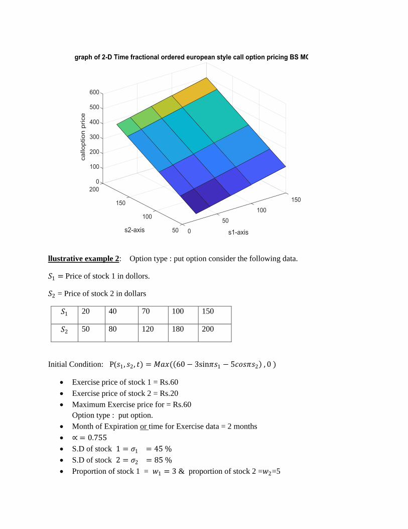
llustrative example 2: Option type : put option consider the following data.
𝑆1 = Price of stock 1 in dollors.
𝑆2 = Price of stock 2 in dollars
𝑆1 20 40 70 100 150
𝑆2 50 80 120 180 200
Initial Condition: P(𝑠1, 𝑠2, 𝑡) = 𝑀𝑎𝑥( 60 − 3sin𝜋𝑠1 − 5𝑐𝑜𝑠𝜋𝑠2 , 0 )
Exercise price of stock 1 = Rs.60
Exercise price of stock 2 = Rs.20
Maximum Exercise price for = Rs.60
Option type : put option.
Month of Expiration or time for Exercise data = 2 months
∝ = 0.755
S.D of stock 1 = 𝜎1 = 45 %
S.D of stock 2 = 𝜎2 = 85 %
Proportion of stock 1 = 𝑤1 = 3 & proportion of stock 2 =𝑤2=5
Risk free rate of return = 03%
Correlation coefficient between Stock 1 and stock 2= 65%
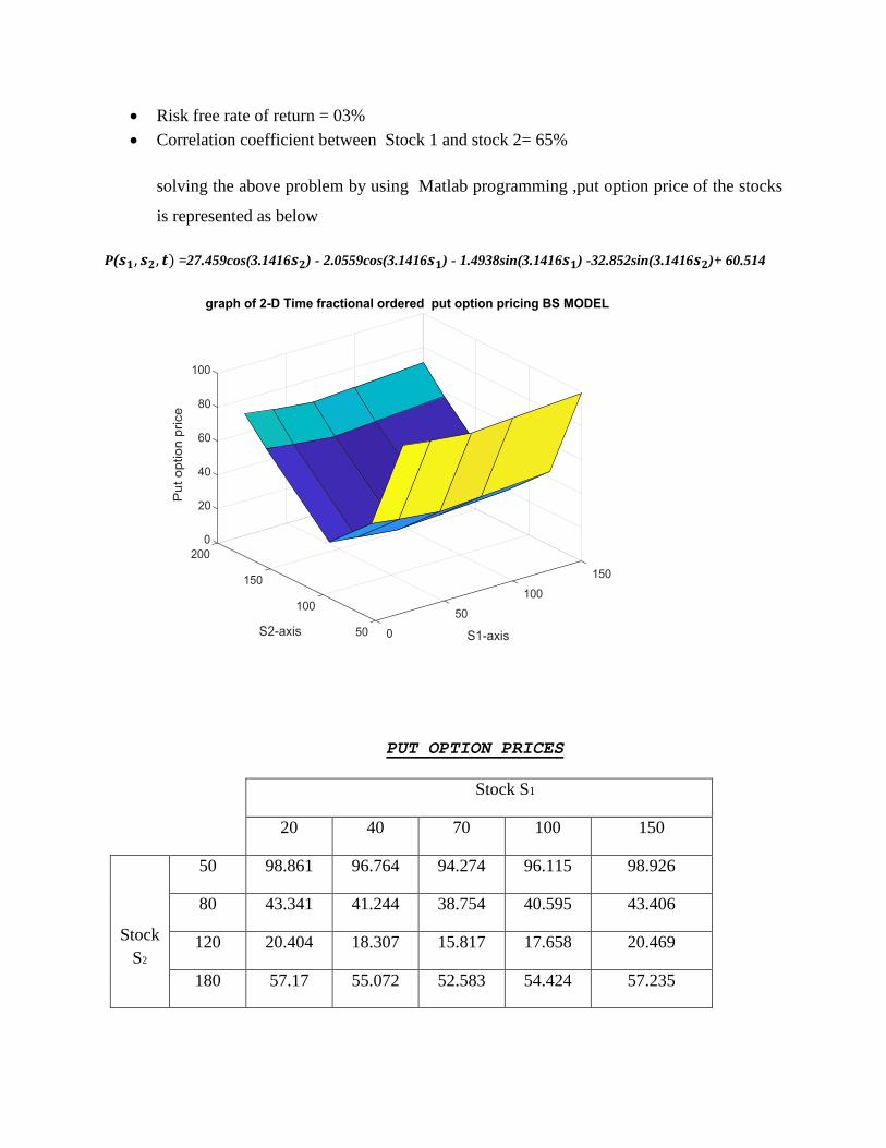
solving the above problem by using Matlab programming ,put option price of the stocks
is represented as below
P(𝒔𝟏, 𝒔𝟐, 𝒕) =27.459cos(3.1416𝒔𝟐) - 2.0559cos(3.1416𝒔𝟏) - 1.4938sin(3.1416𝒔𝟏) -32.852sin(3.1416𝒔𝟐)+ 60.514
PUT OPTION PRICES
Stock S1
20 40 70 100 150
Stock
S2
50 98.861 96.764 94.274 96.115 98.926
80 43.341 41.244 38.754 40.595 43.406
120 20.404 18.307 15.817 17.658 20.469
180 57.17 55.072 52.583 54.424 57.235

200 71.267 69.17 66.68 68.521 71.332
Illustrative example 3: Option type : European call option consider the following data.
𝑆1 = Price of stock 1 in dollors.
𝑆2 = Price of stock 2 in dollars
𝑆1 20 40 70 100 150
𝑆2 50 80 120 180 200
Initial condtion: C(𝑠1, 𝑠2, 𝑡) = 𝑀𝑎𝑥( 2𝑠13 + 5𝑠2
2 , 0 )
Exercise price of stock 1 = Rs.60
Exercise price of stock 2 = Rs.90
Maximum Exercise price for = Rs.90
Option type : put option.
Month of Expiration or time for Exercise data = 2 months
∝ = .125
S.D of stock 1 = 𝜎1 = 40 %
S.D of stock 2 = 𝜎2 = 65 %
Proportion of stock 1 = 𝑤1 = 2 & proportion of stock 2 =𝑤2=5
Risk free rate of return = 07%
Correlation coefficient between Stock 1 and stock 2= 85%
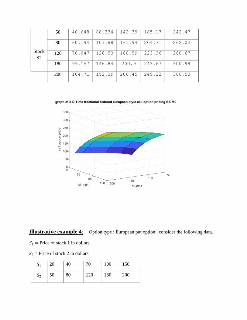
solving the above problem by using matlab programming ,put option price of the stocks
is represented as below
C(𝒔𝟏, 𝒔𝟐, 𝒕)= 2.1517 𝒔𝟏𝟑 + 5.3794 𝒔𝟐
𝟐 - 99.777
Stock S1
20 40 70 100 150
Stock
S2
50 40.648 88.334 142.39 185.17 242.47
80 60.194 107.88 161.94 204.71 262.02
120 78.847 126.53 180.59 223.36 280.67
180 99.157 146.84 200.9 243.67 300.98
200 104.71 152.39 206.45 249.22 306.53
Illustrative example 4: Option type : European put option , consider the following data.
𝑆1 = Price of stock 1 in dollors.
𝑆2 = Price of stock 2 in dollars
𝑆1 20 40 70 100 150
𝑆2 50 80 120 180 200
Initial condtion: C(𝑠1, 𝑠2 , 𝑡) = 𝑀𝑎𝑥(2(𝑥2+𝑦2) - ln(y)+ ln(x)-,0)
Maximum Exercise price for = Rs. 2(𝑥2+𝑦2)
Option type : put option.
Month of Expiration or time for Exercise data = 5 months
∝ = .125
S.D of stock 1 = 𝜎1 = 40 %
S.D of stock 2 = 𝜎2 = 20 %
Proportion of stock 1 = 𝑤1 = 1 & proportion of stock 2 =𝑤2=1
Risk free rate of return = 8%
Correlation coefficient between Stock 1 and stock 2= 75%
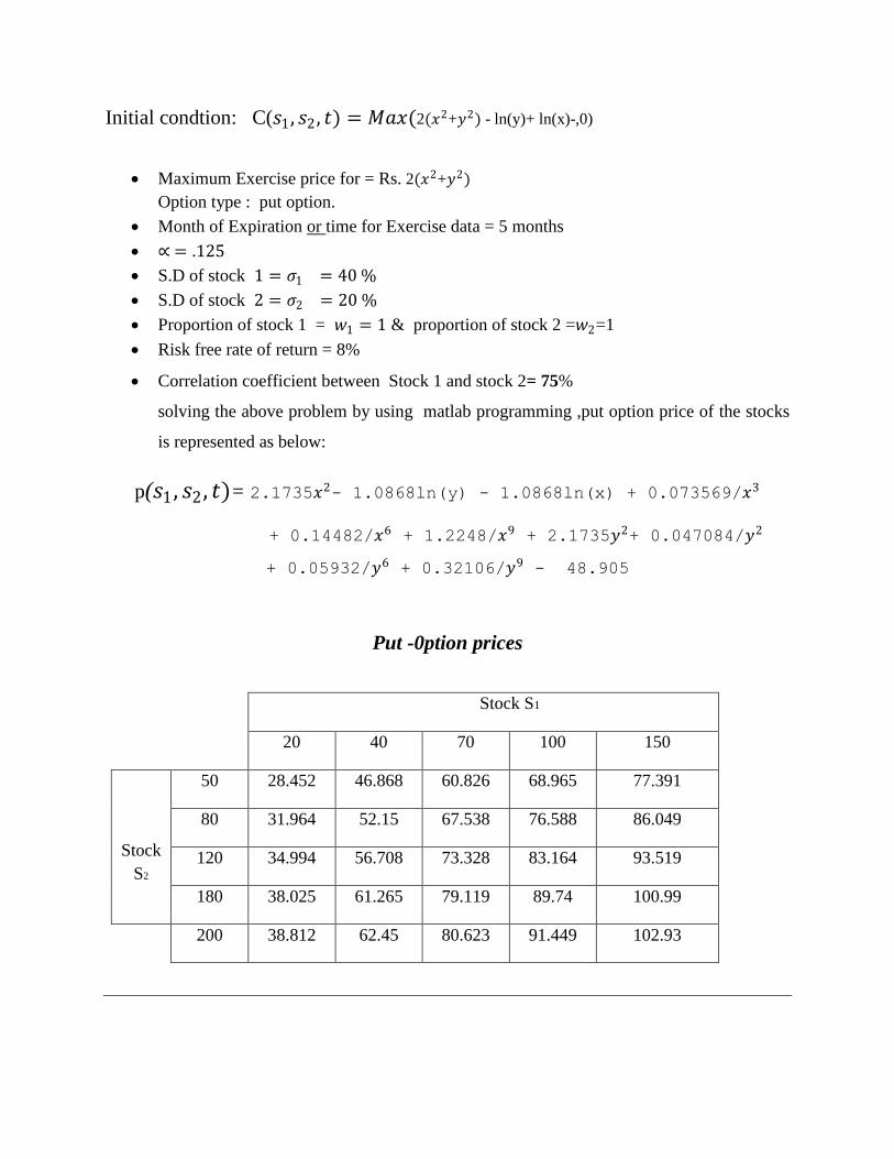
solving the above problem by using matlab programming ,put option price of the stocks
is represented as below:
p(𝑠1 , 𝑠2 , 𝑡)= 2.1735𝑥2- 1.0868ln(y) - 1.0868ln(x) + 0.073569/𝑥3
+ 0.14482/𝑥6 + 1.2248/𝑥9 + 2.1735𝑦2+ 0.047084/𝑦2
+ 0.05932/𝑦6 + 0.32106/𝑦9 - 48.905
Put -0ption prices
Stock S1
20 40 70 100 150
Stock
S2
50 28.452 46.868 60.826 68.965 77.391
80 31.964 52.15 67.538 76.588 86.049
120 34.994 56.708 73.328 83.164 93.519
180 38.025 61.265 79.119 89.74 100.99
200 38.812 62.45 80.623 91.449 102.93

Illustrative example 5: Option type: put option , consider the following data.
𝑆1 = Price of stock 1 in dollors.
𝑆2 = Price of stock 2 in dollars
𝑆1 20 40 70 100 150
𝑆2 50 80 120 180 200
Initial condtion: p(𝑠1 , 𝑠2, 𝑡) = 𝑀𝑎𝑥(-5sin(x)-8y+5xy,0);x)-,0)
Maximum Exercise price for = Rs. 25xy
Option type : put option.
Month of Expiration or time for Exercise data = 5 months
∝ = .125
S.D of stock 1 = 𝜎1 = 40 %
S.D of stock 2 = 𝜎2 = 20 %
Proportion of stock 1 = 𝑤1 = 1 & proportion of stock 2 =𝑤2=1
Risk free rate of return = 8%
Correlation coefficient between Stock 1 and stock 2= 75%
solving the above problem by using matlab programming ,put option price of the stocks
is represented as below:
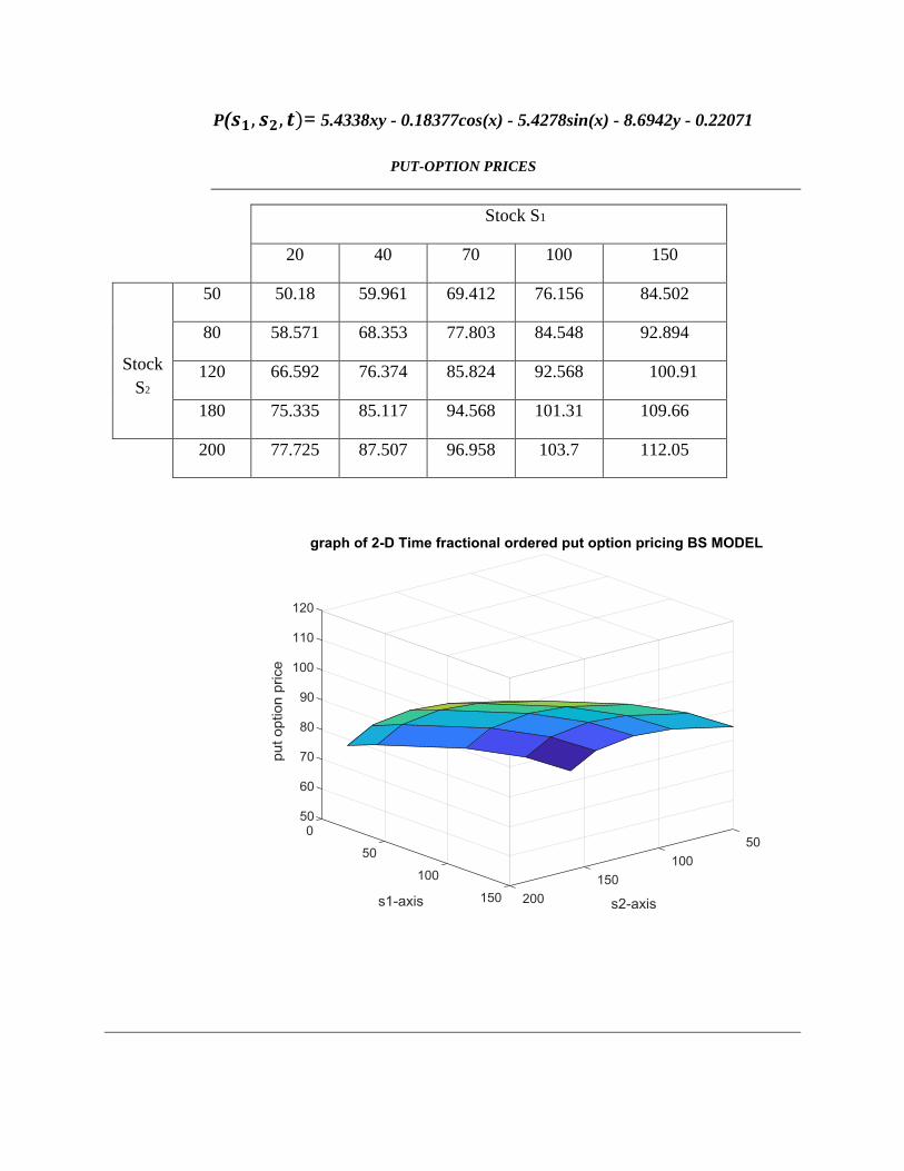
P(𝒔𝟏, 𝒔𝟐, 𝒕)= 5.4338xy - 0.18377cos(x) - 5.4278sin(x) - 8.6942y - 0.22071
PUT-OPTION PRICES
Stock S1
20 40 70 100 150
Stock
S2
50 50.18 59.961 69.412 76.156 84.502
80 58.571 68.353 77.803 84.548 92.894
120 66.592 76.374 85.824 92.568 100.91
180 75.335 85.117 94.568 101.31 109.66
200 77.725 87.507 96.958 103.7 112.05
Concluding Remarks :
In this paper technique of Samudu Transforms and its derivatives and integral properties are
applied to compute analytical solution of time fractional non – linear two dimensional BS PDE
model in form of infinite series to evaluate put options of two stocks asset. Illustrative practical
example is also presented to understand the reliability, efficiency, simplicity, and effectiveness
of the purposed scheme. Samudu Transforms has many powerful and effective techniques to
obtain analytic solution of any type time fractional PDE in least time with less computation.
References
1. K. Zakaria and S. Hafeez, "Options Pricing for Two Stocks by Black – Sholes Time
Fractional Order Non – Linear Partial Differential Equation," 2020 3rd International
Conference on Computing, Mathematics and Engineering Technologies (iCoMET),
Sukkur, Pakistan, 2020, pp. 1-13, doi: 10.1109/iCoMET48670.2020.9073866.
2. Hall John: Options, Future and other Derivatives, 5th
edition prentice Hall.
3. Kwok: Mathematical Models of Financial Derivatives (1998) 62-64
4. P-Vilmot: The Mathematics of Financial Derivatives University press.
5. Shedon Ross: An Introduction to Mathematical Finance Cambridge university press.
6. Bernt: Stochastic D.E; An introduction with application; 5th
edition.
7. Financial Derivatives, Theory concept and problems by S.L. Euptc.
8. G.K Weatuga, Sumudu Transforms, a new integral Transform to solve differential
equations and control engineering problems, Mathematical Engineering 61(1993) 329-
329
9. F-B-M Belagacem, A-A Karbali: and S-L Kala; Analytical investigation of sumudu
transform and integral to production equations, Mathematical problems in Engineering,3
(200) 103-118
10. Sumudu Transform method for Analytical solutions of Fractional Type ordinary
Differential Equations
a. (Hindawi Publication Co-orprations, Mathematical problems for Engineering)
volume 2015-1315 690.
11. H-Eltayeb and Kilichman, A note on Sumudu Transforms and differential equations,
Applied Mathematics Science (2010)- 4(22) 1089-1098.
12. On Sumudu Transforms of Fractional Derivatives and its applications to Fractional
Differential Equations International, Knowledge press: ISSN 2395-4205(P) ISSN-2395-
4213.
13. Asira MA Further properties of Sumudu Transforms and its applications. International
journal of Mathematical education, Science & Technology 2002: 33(2): 441-449
14. Sumudu Transform Method for solving Fractional D.E Journal of Mathematics &
Computer Science 2013; 6: 79-84
15. Computational and Analytical solution of Fractional order Linear Partial Differential
Equations by using Sumudu Transforms and its properties.
IJCNS international Journal of Computer science and Network security Vol 18#9,
September 2018.
16. Basic Properties of Sumudu Transform to some Partial Differential Equations, Sakarya
University Journal of science 23(4), 509-514, 2019.
17. D-Kumar, J Singh, Sumudu Decomposition method for Non- Linear equations,
International Mathematics Forum 7(2012) 515-521.
18. European option Pricing of Fractional Black Sholes model using Sumudu Transforms and
its Derivaties, Refad; general letters in Mathematics Vol1, No.3 Dec 2016 PP:74-80 e-
ISNN 2319-9277
19. Barles, G. and Sooner H.M: Option pricing with Transaction cost and a Non-Linear
Black Sholes Equations. Finance stock 2,4 (1998)- 369-397
20. Black Sholes, M. The pricing of options and co-orprate liabilities 1973, 81,637-654.
21. Misrana, M lub, Fractional Black sholes Model with application of Fractional option
Pricing; International Conference of optimization and control 2010, 17,99-111 (Cross
reference) pp-573-588
22. Tracho; Two dimensional Black Sholes model will European call option. Math
compute.2017,2223(eross reference)

23. Bernet; Stochactic D.E; An introduction with application spoinger 5th
edition
24. Black Sholes Pricing Model; Black Sholes option Pricing Model Bardley University, n.d
web 2016.
